Derivation of Schrödinger’s equation from the Hamilton-Jacobi and the Eikonal equations
Abstract
Most authors of textbooks on quantum mechanics either postulate or sketch a short ‘ad hoc‘ derivation of Schrödinger’s equation. In this work we give a detailed derivation of Schroödinger’s equation from the Hamilton-Jacobi equation and the Eikonal equation in geometrical optics. We start from the historical debates on the nature of light - whether it is a beam of particles, or waves in the aether. We derive the Eikonal equation and show the conditions when a wave can behave as a beam of particles. Then we discuss several experiments with an electron gun, that show clearly diffraction and interference of a single electron. Next, in order to explain these experiments, we derive Schrödinger’s equation by comparing Hamilton-Jacobi equation in classical mechanics with the Eikonal equation in geometrical optics. To do that, we first show how to derive the wave equation from the Eikonal equation (not the other way around!). Second, we use this method to derive Schrödinger’s equation from the Hamilton-Jacobi equation. Next, we derive Born’s statistical rule using the early understanding of de Broglie that both particles and waves exist. Afterwards, we show that historically people preferred to remove the particles (as well as their trajectories) altogether from de Broglie’s ideas but retained Born’s rule (the so called Copenhagen interpretation). These derivations of the foundations of quantum mechanics do not follow precisely the history of the subject. Rather we select some early ideas and experiments in a judicious manner to present Schrödinger’s equation in a logical and ordered way. We use the electron gun experiments instead of black body radiation and photoelectric effect. Our derivation may bring more light and satisfaction for the undergraduate students about the confusing and rather mysterious subject of quantum mechanics.
I Introduction
Many textbooks on quantum mechanics do not derive Schrödinger’s equation but simply postulate it (for instance Griffiths2018 and Tannoudji2019 ) and proceed directly to applications. Other textbooks use de Broglie’s idea that free particles with momentum p and energy are ‘associated‘ with plane waves: , where is Planck’s constant and is the amplitude of the plane wave. Next, they state Born’s rule. Then they use the correspondence principle as well as the principle of superposition, and by building wave packets, they Bohm1989 ; Messiah2014 ; Greiner2001 ; Dirac1959 reach the conclusion that to obtain the average momentum, we need to calculate the integral:
| (1) |
where is the whole of space. This ‘derivation‘ of the momentum operator is similar to what is done in Landau1981 , where the authors derive the momentum operator from symmetry considerations. Once the operator of momentum is derived, some authors Griffiths2018 ; Greiner2001 simply postulate that for a general power :
| (2) |
Then, they ‘derive‘ the Hamiltonian: and postulate Schrödinger’s equation
| (3) |
Other authors Bohm1989 ; Messiah2014 use the correspondence principle and guess what the Schrödinger’s equation ought to be. Others Landau1981 ; Dirac1959 reach the conclusion that in the semi-classical regime, the wave function is:
| (4) |
where is the action in classical mechanics. After some semi-classical arguments Landau1981 and Dirac1959 guess Schrödinger’s equation.
In this paper we derive in detail Schrödinger’s equation by comparing Hamilton-Jacobi equation and the Eikonal equation in geometrical optics Sommerfeld1964optics ; Born1999 . We first show the conditions when a wave behave as a beam of particles. These conditions follow from our derivation of the Eikonal equation from the wave equation. Then we argue that Hamilton-Jacobi equation is a type of Eikonal equation, which should follow from some unknown wave equation. Next, we invent a specific mathematical procedure that allows us to derive the wave equation from the Eikonal equation (not the other way around!). We use this procedure to derive Schrödinger’s equation from Hamilton-Jacobi equation. As far as the author knows, this particular derivation has not been made before. People have only speculated on the similarity between the Eikonal equation and the Hamilton-Jacobi equation Landau1981 ; Dirac1959 but to our knowledge, a specific derivation of this type has not been made.
This paper is organized as follows. In Section II we give a very brief history of the corpuscular vs wave theory of light. In Section III we show when waves behave as a beam of particles. In Section IV we derive the time-dependent Eikonal equation. In Section V we consider three electron gun experiments, which clearly show diffraction and interference of single electrons. In Section VI we derive Hamilton-Jacobi equation in classical mechanics. In Section VII we compare Hamilton-Jacobi equation and the Eikonal equation (Table I) and we invent a procedure which allows us to derive the wave equation from the Eikonal equation. We use this procedure to derive Schrödinger’s equation from the Hamilton-Jacobi equation. In Section VIII we continue with the history of the Schrödinger’s equation and compare the original de Broglie’s idea (pilot wave theory) with the Copenhagen interpretation. We show that people discarded the particles and their trajectory, but postulated collapse of the wave function. For completeness sake we derive Born’s rule in pilot wave theory and show that pilot wave theory can also explain the three electron gun experiments. Section IX gives the conclusions.
II What is light - very short history
II.1 Light as particles
One of the most influential persons in the history of physics is Descartes. Perhaps his major contribution was his idea that all of physics can be reduced to mechanics Whittaker1989 , including optics and gravity. For instance, his understanding of the solar system was that the empty space was filled with an invisible substance called ‘aether‘. The sun was considered to be at the center of a giant aether vortex, which sweeps along the planets. Descartes and his followers had employed this idea to understand gravity, electricity, magnetism and optics.
When it comes to light, people devised two competing theories - light was considered either as particles (corpuscules) or as vibrations in the aether, similar to the sound, which is vibrations in the air.
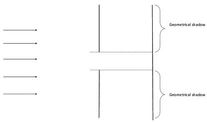
Newton (though he was a believer in the aether Whittaker1989 ) considered light as particles, not waves. His reasoning was that it is very difficult to explain the rectilinear motion of light, if it was waves in the aether. Indeed, let us consider a light beam that travels through a small aperture as shown in FIG. 1. Newton said that light never entered the geometrical shadow (he was wrong about that). This rectilinear motion of light resembles a beam of particles, not waves.
Even more, it is not very difficult to explain Snell’s laws of refraction as well as the law of reflection of light using Newton’s law of motion. Indeed, let us imagine particles of light passing through a medium 1 to medium 2, as shown in FIG.2.
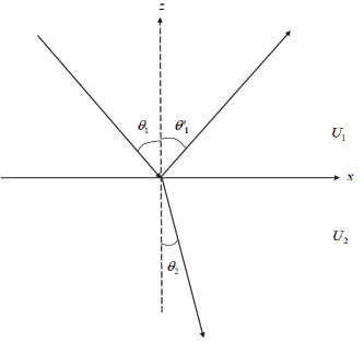
At the boundary we assume that a force F acts on the light corpuscles. We also assume that the force has a potential . In the first medium the potential is , while in the second medium it is , and . Then, since the potential energy changes in the direction only, the force F also is in the direction. Then the momentum in the direction is conserved for both reflected and refracted light particles. If we apply the law of conservation of energy and of for the reflected light particles we have:
| (5) |
where is the mass of the hypothetical light particles, and and are the velocities of incident and reflected light particles. It follows that the magnitude of these velocities are the same, i.e. . The law of conservation of leads to:
| (6) |
From Eqs. (5) and (6) we have that and thus . This is the familiar law of reflection of light.
Now, let us consider Snell’s law of refraction. The law of conservation of energy leads to:
| (7) |
Here is the velocity of refracted light particles. Now, obviously from Eq. (7) we see that . From the law of conservation of we have that:
| (8) |
from which we obtain:
| (9) |
The ratio depends only on the nature of the two media, as is Snell’s law.
We have now two powerful reasons in defense of the corpuscular theory of light - rectilinear motion of light (no penetration of light into the geometrical shadow) as well as simple explanation of the laws of reflection and refraction.
We shall now see how the wave theory can account for these facts.
II.2 Light as vibrations in the aether
Hook Whittaker1989 considered light as vibrations of the aether. He considered a single pulse that falls on the boundary between two media, as shown in FIG. 3. This vibration may be anything - it may be displacement of the aether particles, or may be contractions of its density, etc. People did not specify what kind of wave in the aether it was.
Now, if , the point will move a shorter distance than point for the same amount of time, i.e. . Then, the new wave front in the second medium will be inclined in a different angle than the angle of incidence. Hook did not derive any equations but his account gives a hope that wave theory of light might be able to describe refraction of light. Note however that in Hook’s theory, if , the refracted light will be inclined toward the normal to the dividing boundary. This result is opposite to what Eq. (9) would tell us.
Huygens established the principle that bears his name. This principle allows for the wave theory of light to answer all of Newton’s objections Whittaker1989 and even to derive the laws of reflection and refraction.
Indeed, it is well known that, according to Huygens’ principle each point of the aether is a source of secondary spherical waves and the new wave front is just the envelope of these secondary wavelets.
In FIG. 4 we see how each point of a plane wave impulse creates secondary wavelets and the new wave front is again a plane. But Huygens’ principle tells us much more. For instance, let us examine a pulse that passes through an aperture, as shown in FIG. 5.
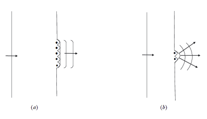
If the wave falls on a larger aperture, using Huygens’ principle the new wave front is still almost a plane. However, if the aperture is very small, the new wave front is almost a circle and the light no longer moves in a rectilinear way. This phenomena, in which waves penetrate into the geometrical shadow by deviating from rectilinear motion is called diffraction. Now, finally Huygens can explain why light can move in a rectilinear way, as if a beam of particles. Perhaps ordinary apertures, through which light usually passes are just too large, as in Fig. 5 (a). Huygens principle tells us that if we have smaller apertures, light will penetrate into the geometrical shadow. Huygens’ principle cannot tell us how small apertures should be but nonetheless it predicts the phenomena of diffraction for small apertures. But more importantly Huygens’ principle can in principle explain why light waves move in a rectilinear way and for large apertures do not penetrate into the geometrical shadow.
Huygens’ principle not only answers Newton’s objection and can explain the rectilinear motion of light but it can also derive the laws of reflection and refraction.
Indeed, let us examine a wave impulse that falls on the boundary between two media, as shown in FIG. 6 and FIG. 7.
We assume that the speeds of light and in these two media are different, i.e. . This may be explained by the fact that perhaps the aether’s density or the ather’s elasticity is different in the two media. Whatever the explanation, it is quite obvious that one can easily imagine why . In addition, we also assume that without loss of generality, , where is the speed of light in vacuum.
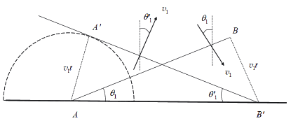
We start with the law of reflection (FIG. 6): as the point reaches the boundary between the two media, at point a spherical wave is emitted (according to Huygens’ principle). After some time point reaches the boundary at point . Obviously, after this time, , while the radius of the sphere becomes . It is obvious then that . Then, the rectangular triangles and are congruent and then . On the other hand, the angles and are the angles of incidence and reflection. Then we have derived the law of reflection, that is the equality of the angles of incidence and of reflection.
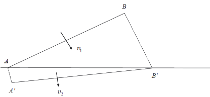
If we use Huygens’ principle we can also prove Snell’s law of refraction. Indeed, let us examine a light pulse that passes through a medium 1 to a medium 2, as shown in FIG. 7.
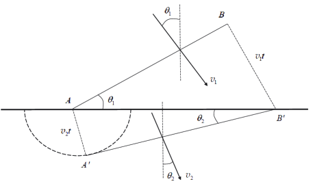
As point reaches the boundary, a spherical wave is emitted. After some time point reaches the boundary and the distance it has traveled is . For the same amount of time, the radius of the spherical wave with center has become . Now, obviously
| (10) |
On the other hand
| (11) |
We divide both Eqs. (10) and (11) and we obtain:
| (12) |
The ratio depends only on the nature of the media, i.e. on the velocities and which are determined by the type of media only. This is just Snell’s law. Note that Eq. (12) is quite the opposite of Eq. (9).
If we define the indexes of refraction: and , where is the speed of light in vacuum, then Eq. (12) becomes:
| (13) |
This is the familiar way Snell’s law is written in textbooks.
In other words, the wave theory of light can also explain reflection and refraction.
Finally, due to the works of Young and Fresnel on the interference and diffraction of light, as well as the successful explanation of the phenomena of double refraction and polarization, wave theory finally triumphed in the 19th century Whittaker1989 .
III How to describe waves
III.1 Plane waves
Huygens’ principle was just a heuristic device to try to make intuitive sense of how waves propagate. Nowadays we know how waves propagate, since the mathematics of waves is way better understood.
Let us consider some function (it may be pressure distribution, or density distribution, or component of electric or magnetic field, etc.), that moves with some speed .
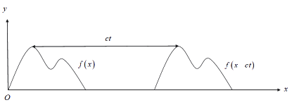
Then, after some time , the function is translated to a distance (FIG. 8). The translated function becomes . The most familiar wave is the cosine function: , which after a distance repeats itself. This is the familiar wavelength. After time the wave becomes:
| (14) |
If we substitute
| (15) |
we have for the moving cosine:
| (16) |
The meaning of is obvious. Let us fix our attention at some particular point with a coordinate . As the wave propagates to the right, the function repeats itself at this particular position after a time . Then is the familiar period of the wave, and that is why is called frequency of the wave. In other words tells us how frequently the function repeats itself at some fixed point . The argument is called phase of the wave. Since the function cosine is periodic, points with phase difference for any arbitrary integer are disturbed in the same way, since the function has the same value for these points.
Let us examine the function . At time and position the phase is . What is the new coordinate of the point, which will have the same phase at the next moment . It is easy to determine:
| (17) |
From this equation we have:
| (18) |
In other words, the point with a fixed phase, moves with a velocity (phase velocity):
| (19) |
In a similar way, we can examine a 3D wave:
| (20) |
We have introduced the wave vector: and the position vector . It is easy to find all points with the same phase at some fixed moment :
| (21) |
But since is fixed, i.e. , we have that
| (22) |
But this is an equation of a plane. Recall that is an equation of a plane, with a normal vector . Similarly Eq. (22) tells us that all points with the same phase (the so called phase surface, or wave front) lie in a plane, with a normal vector k, as shown in FIG. 9. That is why the wave, described by Eq. (20) is called a plane wave.
Let us examine how the phase surface (the plane) moves. After a time interval , the plane with the same phase has moved to a new position, as shown in FIG. 9. Let us translate point along the vector k to the new plane in point (see FIG.9). The length is the distance . We can easily calculate the speed necessary for point to move to point . We have that the phase is the same for both surfaces, i.e.
| (23) |
Simplifying we have:
| (24) |
But we can group , and into a vector and this equation is transformed to:
| (25) |
But then . Then we have
| (26) |
Then we can find the phase velocity
| (27) |
If the wave front moves in a medium with index of refraction , then the same reasoning gives:
| (28) |
III.2 Arbitrary wave
Let us consider now an arbitrary function, with a fixed frequency:
| (29) |
Here is just an arbitrary phase of the function . For a plane wave, . But in the genral case (29) can be quite arbitrary.
The function is still periodic in time with a period . Now, the question is: when this function is a wave? For plane waves it was very easy to discover the condition, when the functions (16) and (20) are actually waves. It was necessary that . But it is more difficult to establish such a condition for arbitrary waves, like (29). Fortunately we know the correct way to discover whether a function is a wave. It has to obey the wave equation (this is our definition of a wave):
| (30) |
where is the speed of light in the medium with index of refraction . If we substitute in the above equation we have:
| (31) |
Now, it is very easy to confirm the condition when the simple functions (16) and (20) are really waves in the particular medium. If we substitute (16) and (20) into the above wave equation we see that the condition for waves is: , as expected. Then in order to discover when the more complicated (29) is a wave, we also have to substitute it into the wave equation (31).
Before we do that, let us calculate the phase velocity of the arbitrary wave (29). Let us consider all points with the same phase, i.e. . When we select a specific moment of time , i.e. , then all points with the same phase are such that: . This is an equation of arbitrary surface, not necessarily a plane, as shown in Fig. 10.
After time , the phase surface has moved. We can easily find the phase velocity. Indeed, we have that the two adjacent surfaces have the same phase if:
| (32) |
We Taylor expand and we have:
| (33) |
(we do not use approximate sign, since we consider infinitesimal quantities). If we group , and into a vector and if we use the gradient of : , we can reduce the above equation to:
| (34) |
Now, it is well known that is normal to the plane Boas2005 ; Nearing2010 . If we select points and in such a way, that is also normal to the plane, then . Then and Eq. (34) becomes:
| (35) |
From this equation we can finally calculate the phase velocity:
| (36) |
One might expect that the condition for the function (29) to be wave is that
| (37) |
But this is wrong! We shall see that condition (37) is not a condition for to be a wave. It is a condition for something else entirely. Indeed, in order for (29) to be a wave, it has to obey the wave equation (31). That is the true condition. We shall later substitute (29) into the wave equation (31) and we shall see that there will be some derivatives of the amplitude as well as second derivatives of . No such derivatives are seen in Eq. (37). Thus we see that the simple condition (37) will not suffice as in the case of plane waves! Condition (37) is not a condition for to be a wave, but for something else.
We shall prove that condition (37) is a condition for the wave to behave as a beam of particles! Indeed, if (37) is true, and if the index of refraction (which is the most frequent case), the phase points of a plane wave will move in straight lines (rays), since when , then (37) implies that . In this way the phase points will move in straight lines and will never penetrate into the geometrical shadow.
Usually people prefer to square (37) and we have
| (38) |
This is the very famous Eikonal equation. This is the condition for waves to behave like a beam of particles. This regime, when light obeys the Eikonal equation is called geometrical optics. People usually use Eq. (38) to find the rays in the case when change from point to point. This shows that even in geometrical optics, light can penetrate into the geometrical shadow, so long as is a function of , and . However is almost always true in everyday experience.
Now, what is left is to check if it is possible for the function (29) to actually obey the Eikonal equation (38). To this end we shall substitute (29) into the wave equation (31). But first, in order to make the calculation simple, we shall use complex notation:
| (39) |
where is a complex wave:
| (40) |
We shall rewrite the wave equation into:
| (41) |
We have that:
| (42) |
Now, let us assume that for some reasons (which we shall investigate below), the third term is much larger than the others. Then we have
| (43) |
In this special regime the wave equation becomes:
| (44) |
Simplifying:
| (45) |
When we cancel , we finally obtain the Eikonal equation:
| (46) |
But if the Eikonal equation is true, a wave can behave as a beam of particles. And we now finally see the conditions for that – it must be the case that the term in Eq. (42) as well as the term should be much larger than all other terms in the wave equation. What is left then is to find out what is the physical meaning of these terms being the largest.
Imagine we have two very close wave fronts, such that the phase difference between them is , similar to FIG. 10. However, for these two surfaces we shall call the distance , and it will correspond to the wavelength of this wave. Then we have:
| (47) |
Taylor expanding we have:
| (48) |
Which is the same as:
| (49) |
But again we have that and . Then we have:
| (50) |
In that case we finally see the meaning of :
| (51) |
simply corresponds to the wave vector k for plane waves. The only difference is that this time the wave vector depends on , and , i.e. we have position dependent wave vector k. This will lead also to position dependent wavelength . If is much greater than all other terms in Eq. (42), it means that the wavelength is quite small. In this way we reach the conclusion that for sufficiently short wavelengths, we have the regime of geometrical optics and no penetration in the geometrical shadow (if the index of refraction ).
The term , where is the distance the wave has traveled in one period. People are used to think that , but this is true only for plane waves or in the regime of geometrical optics. Indeed, the Eikonal equation can in fact be rewritten as . Just substitute and into the Eikonal equation Eq. (38) (or (37)) and the result immediately follows.
One last point. It is easy to see that if the phase is sufficiently large (to be made more precise below), then this would effectively lead to the regime of geometrical optics. Indeed, let us substitute . Here , while . In that case is very large. If we substitute into Eq. (42), the terms in the brackets become:
| (52) |
The largest of the terms in the brackets is the term with . Then for large (small ) we have the regime of geometrical optics.
IV Time-dependent Eikonal equation
So far, we have considered an arbitrary wave with the same frequency in Eq. (29). We will consider now even a wave, which has arbitrary time dependence:
| (53) |
In order to calculate the phase velocity in this case, we take two points and (see FIG. 10), such that again . The two phases are the same, i.e.
| (54) |
After Taylor expanding, we obtain:
| (55) |
Since , we have that:
| (56) |
Again, in order for the wave front to move like a beam of particles, we expect that
| (57) |
Then, this reduces to:
| (58) |
When we square, we have:
| (59) |
This is the new condition for geometrical optics.
It is not very difficult to prove that if and are sufficiently large, the wave equation is reduced to the Eikonal equation (59). Indeed, if is quite small, from Eq. (42) is again reduced to (43). In addition:
| (60) |
If the last term is the largest:
| (61) |
Finally if we substitute this equation and Eq. (43) into the wave equation (41), we obtain again the Eikonal equation (59). Therefore arbitrary waves with arbitrary time dependence may behave as a beam of particles.
Finally, the meaning of is analogous to the frequency, but this time position and time dependent. Then gives the distance the wave travels for one period at position at time . Sufficiently small wavelengths and or sufficiently large will lead to the regime of geometrical optics and to Eq. (59).
V Electron gun experiments
In this section we shall present the electron gun and shall introduce the effects of interference of electrons. We shall follow Maudlin2019 . These are however hypothetical experiments. For real experiments see Refs. Frabboni2007 and Frabboni2008 .
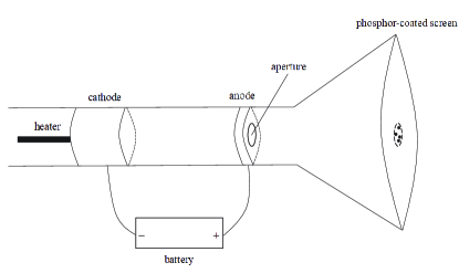
Each battery has a positive and a negative end. These ends are called electrodes. The positive electrode is called an anode, while the negative is called a cathode. Let us connect the two ends of the battery with wires to two metal plates (see FIG. 11). Also, let us make aperture in the plate, connected to the anode, and behind the anode we place phosphor-coated screen.
Experiment 1: When the cathode is very hot (due to the heater), we see on the screen a bright spot. However, if we turn down the heater, the spot gets dimmer and dimmer. If we continue to turn down the heater even more, instead of a spot, individual flashes appear on the screen, in exactly the same place, where the spot was (FIG. 11). If we continue to turn down the heater even further, the flashes appear one at a time with a great interval of time between them. The individual flashes are obviously particles. These are the familiar electrons.
Experiment 2: We place a barrier after the anode with a single narrow slit (see FIG.12).
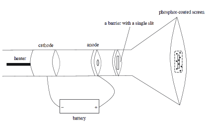
We see that the bright spot initially is just as narrow as the shape of the slit. But making the slit even thinner, the thin spot on the screen gets wider and spread out. This phenomenon is the familiar diffraction. However, even when we turn down the heater, such that only individual flashes appear, they nonetheless appear on exactly the same place, where the diffracted and widened spot was (FIG. 12). This shows that there is a diffraction even with individual flashes. This is unexpected. Indeed, diffraction makes sense for waves, but not for individual flashes.
Experiment 3: We place a barrier after the anode with two slits (the famous double slit experiment), as shown in FIG.13.
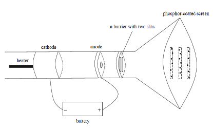
We see that for sufficiently thin slits, the bright spot on the screen has interference bands - regions of extremely high intensity alternating with quiescent regions. So far, this is not striking. Interference phenomena are quite familiar. However, the striking thing is that even in the case, when we turn down the heating element, such that only individual flashes appear, they nonetheless appear only where the interference maximums are, and never at the location of the interference minimums (FIG. 13). This is striking, since interference makes sense for waves, but not for individual flashes.
We shall try to explain these three experiments by using modified ideas of de Broglie (modified by Bohm Bohm1952 ; Bohm1995 ; Norsen2017 ). He thought that the particles are guided by waves. This is the famous pilot wave theory. In other words, de Broglie thought that there are both particles and waves. For each particle, there is attached a particular wave, that somehow guides the particle. Particles are never guided to the interference minimum of the wave and more frequently to the interference maximums. Later people removed the particles and their trajectories and only the wave was left. The individual flashes were explained with a sudden collapse of the wave. This was done for reasons of parsimony - in the new theory there are fewerg structures - just a wave and no particles. This theory with only a wave is called Copenhagen interpretation. To this day, pilot wave theory is the best rival of the Copenhagen interpretation Norsen2017 . However, we do not wish to enter into a dispute about interpretations. We shall simply follow history. For the time being we shall adopt de Broglie’s pilot wave theory (perfected by Bohm) and later we shall remove the particles and their trajectories, following Copenhagen interpretation (since we follow the historical development).
The question is this: How can we attach a wave that guides a single particle, such that the three experiments can be explained? We shall make a short and quick review of classical mechanics and of the principle of least action. Later, we shall be able to attach a wave to each particle by comparing the equation for the action of the particle with the Eikonal equation. This comparison will help us to derive the wave equation for these waves, called Schrödinger’s equation.
VI The Principle of Least Action
Let us examine a single particle moving in 1D (later we shall generalize to 3D motions). It is well known that as the particle moves, it selects that law of motion, for which the action is stationary Sommerfeld1964 . The action is given by:
| (62) |
where is the Lagrangian of the particle. Here is the kinetic energy of the particle, while is the potential energy. It is well known that the Lagrangian must obey the famous Euler-Lagrange equations Sommerfeld1964 for to be stationary:
| (63) |
The overline in designates the true law of motion unlike all other virtual motions . This equation holds true only when . In order to derive this equation, people usually consider small virtual deviations from the true trajectory Sommerfeld1964 . In that case there is only one true trajectory, and a lot of virtual trajectories.
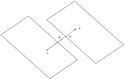
Let us now consider a different scenario. Instead of one real trajectory and many virtual trajectories, we consider only real trajectories. For instance, we depict two real but close trajectories and in FIG. 14.
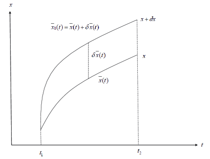
At the final moment , and . The action will be different at points and , since it is calculated along different (though real) trajectories and . In order words, the action will become a function of . In that case we have:
| (64) |
On the other hand we have:
| (65) |
We have Taylor expanded . We also take into account that
| (66) |
We integrate by parts the second term in Eq. (65):
| (67) |
Now, we know that . It well known Sommerfeld1964 that the momentum of the particle at the point is:
| (68) |
In that case Eq. (67) becomes:
| (69) |
We substitute Eq. (69) into Eq. (65) and we obtain:
| (70) |
The last integral however is , since for the true motion the Lagrangian obeys Euler-Lagrange equations (63). Then we finally have:
| (71) |
By comparing with Eq. (64) we finally have:
| (72) |
If the motion were 3D, it is easy to show in the same way that: , and . In vector form, we have:
| (73) |
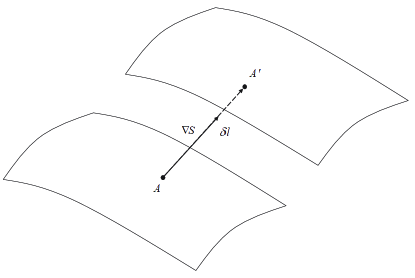
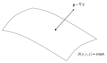
In other words, if we can calculate the function we can always calculate the momentum p of the particle, if it passes through the point . It is normal to the level-surface , as shown in FIG. 15.
In order to derive the equation for , we shall use the law of conservation of energy: . We rewrite it in the form:
| (74) |
We then substitute into this equation and we obtain:
| (75) |
This is Hamilton-Jacobi equation for a beam of particles with the same energy . We could in principle construct many such surfaces and from them we can construct the trajectory of any particular particle, using the condition .
However, we can generalize this result. We may consider real trajectories even for different moments in time and not just different points and (see FIG. 16).
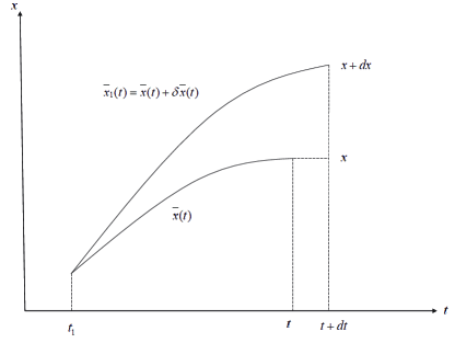
The action is the action that corresponds to the trajectory , while the action is the action that corresponds to the other real trajectory . Here the real trajectory is close to the other real trajectory . Since in this case the action is function of both space and time we have:
| (76) |
On the other hand,
| (77) |
The first integral is:
| (78) |
We substitute (78) into (77) and we have:
| (79) |
The integral in this equation can be integrated by parts in the same manner as we did the integral in Eq. (65). Then in analogous way we derive:
| (80) |
But again, is the momentum of the particle, while the integral in this equation is (the Lagrangian for the true law of motion obeys Euler-Lagrange equations). Then, if we substitute (80) into (79) we derive:
| (81) |
We transform the last term:
| (82) |
However, the last two expressions are second order and we can ignore them. Then we have that:
| (83) |
When we substitute this result into Eq. (81) we obtain:
| (84) |
We wish to connect with . Note that (FIG. 16) but it is easy to see that:
| (85) |
In that case we have:
| (86) |
We substitute this result into Eq. (84) and we finally have:
| (87) |
It is well known Sommerfeld1964 that the term in the brackets is the energy of the particle. Then we finally have:
| (88) |
If the motion were 3D, in an analogous manner we would have obtained:
| (89) |
In other words,
| (90) |
This leads us to conclude that:
| (91) |
as well as:
| (92) |
If we plug these results into the energy conservation law , we have:
| (93) |
This is the famous Hamilton-Jacobi equation Sommerfeld1964 .
VII Comparison between the Eikonal equation and the Hamilton-Jacobi equation. Derivation of Schrödinger’s equation
VII.1 Comparison between the Eikonal equation and the Hamilton-Jacobi equation
The attentive reader may have noticed quite a great resemblance between the Eikonal equations (38) and (59) on the one hand and the Hamilton-Jacobi’s equations (75) and (93) on the other. We can also see this comparison in Table I.
| optics | mechanics | |
|---|---|---|
| Wave Equation | ? | |
| regime of | ||
| no dependence | ||
| regime of | ||
| dependence |
Now, when we examine Table I and consider the resemblance between the Eikonal equations of geometrical optics and Hamilton-Jacobi equations in Newtonian mechanics, it is quite natural to ask the following question: is it the case that the Hamilton-Jacobi equations (which reproduce the familiar Newtonian mechanics) are just the regime of of some yet unknown wave equation? In other words, could it be the case that the Hamilton-Jacobi’s equations are the Eikonal equations of some unknown wave equation? And can we find out what this wave equation is? Perhaps this wave equation can explain somehow the electron gun experiments with interference and diffraction of single particles!
When we compare the Eikonal equations with the Hamilton-Jacobi equations (Table I), we see that the action resembles a phase of unknown wave. Then, if we designate the unknown wave with , it is tempting to postulate that: , where is the action in classical mechanics. However the action has units of energytime, while the phase of any wave should be dimensionless. Therefore, the unknown wave ought to be of the form:
| (94) |
Here is some quantity that should have a dimension of action. Only then is dimensionless. It will turn out (see below) that is the familiar Planck’s constant. We also expect that the unknown wave equation for will be reduced to the Hamilton-Jacobi equations when . Indeed, we have shown in Eq. (52) that for large phases of the waves (in our case ), the wave equation is automatically reduced to the regime of . In other words, we shall treat the condition as equivalent to .
But even in the regime () the yet unknown wave will not give individual flashes. Indeed, the regime () simply says that a parallel beam (which may be very thick) of the wave moves in a rectilinear way (as in the case of geometrical optics). If we are to have individual flashes we need more. In order to explain the individual flashes, De Broglie thought that there are both particles and waves. The individual flashes are the particles, which are guided by the phase of the wave in this manner: if we somehow know the wave and its phase , we can calculate the momentum p of the particle by the guiding equation .
Summary: De Broglie’s idea to explain the electron gun experiments with interference and diffraction is this: To each particle, attach a wave and guide the particle by the guiding equation: . The wave will obey some yet unknown wave equation. In the limit (), the unknown wave equation will be reduced to its Eikonal equations, which are in fact the Hamilton-Jacobi equations shown in Table I. This regime of () then will give us the familiar Newtonian mechanics. However, we hope that if we are not in the regime (), the wave will guide the particles in such a way, that the electron gun experiments with interference and diffraction can be explained. What is left then is to find the unknown wave equation for .
Before we do that, let us transform the guiding equation . Let us take :
| (95) |
Then is given by:
| (96) |
We have used the fact that for any complex number , . The particle’s velocity is then given by:
| (97) |
VII.2 Derivation of the wave equation from the Eikonal equation
Thus far we were able to derive the Eikonal equations of geometrical optics from the wave equation of wave optics (see Table I). Now we wish to do the opposite procedure: from the Eikonal equations of geometrical optics we shall guess what is the wave equation of wave optics. This will be important for us later when we derive Schrödinger’s wave equation for the wave .
Let us consider a complex wave of the type:
| (98) |
We pretend that we do not know the wave equation for , Eq. (41). We only know that the phase obeys the time-dependent Eikonal equation (59):
| (99) |
This equation is the regime of geometrical optics of the unknown wave equation. This regime means that the phase is quite large and is of the type:
| (100) |
where , while . Then .
Let us take the following derivative:
| (101) |
In the limit of geometrical optics, the last term is of the order of and is thus the largest. In that case we can ignore the first term and we get:
| (102) |
In other words, we can replace:
| (103) |
In the same way it is very easy to prove that for the square of the first derivative we have:
| (104) |
Indeed, we have
| (105) |
In the geometrical optics regime, the last term is the largest, since it is of the order of . Then, we can ignore all other terms and we get:
| (106) |
which proves Eq. (104). Eq. (104) is also valid for the other derivatives , and the time . With this preparation at hand, let us start with the time-dependent Eikonal equation in geometrical optics (99), written with partial derivatives:
| (107) |
We recall that we pretend we do not know the wave equation (41). We wish to guess it from the above equation. To this end, let us multiply the above equation with :
| (108) |
Since, the above equation is the limit of geometrical optics, we can use approximation (104) and then Eq. (108) is transformed into:
| (109) |
If we substitute , the above equation is reduced to:
| (110) |
After some rearrangement, this is precisely the wave equation:
| (111) |
It is amazing, that we were able to guess what is the wave equation from the Eikonal equation. Now we shall follow the same procedure to derive the unknown wave equation for out of Hamiton-Jacobi equation.
VII.3 Derivation of Schrödinger’s equaiton
We consider a wave of the type:
| (112) |
We do not yet know the wave equation for . But we know that in the regime of ’geometrical optics’ (i.e. Newtonian mechanics), i.e. when the unknown wave equation is reduced to its ’Eikonal equation’, i.e. to Hamilton-Jacobi equation:
| (113) |
The regime of ’geometrical optics’ (i.e. Newtonian mechanics) , means that the Planck’s constant is really small. In this regime of , we have:
| (114) |
We have left only the largest term of order .
In other words, we have the following approximation (valid only when ):
| (115) |
In the same way, it is trivial to show that for the square of the derivative we have:
| (116) |
Now, that we have these approximations, we are finally ready to derive Shrödinger’s equation from the Hamilton-Jacobi equation. Indeed, let us start with the Hamilton-Jacobi equation (113) in terms of derivatives:
| (117) |
We multiply both sides with the complex wave :
| (118) |
Next, we use our approximations Eqs. (115) and (116) but also for , and derivatives and Eq. (118) is transformed into:
| (119) |
After we simplify and we substitute we finally have the famous Schrödinger’s wave equation:
| (120) |
It is this equation that in the regime of ‘geometrical optics‘ is reduced to the Hamilton-Jacobi equation (113).
VIII Copenhagen interpretation vs Pilot Wave theory
VIII.1 Copenhagen interpretation
We finally have the complete pilot wave theory of de Broglie-Bohm. We start with the Schrödinger’s equation for the complex wave :
| (121) |
which guides the particle by the guiding equation:
| (122) |
If we know the initial position of the particle and the initial wave function we can in principle solve Schrödinger’s equation (121) and from the guiding condition (122) we can determine the trajectory of the particle. We have not yet shown that this theory can explain the electron gun experiments (it can). However, in the limit of geometrical optics , Schrödinger’s equation is reduced to the time-dependent Hamilton-Jacobi equation (113) and given the guiding condition Eq. (122) we restore the standard classical Newtonian physics.
However, for various historical and philosophical reasons Norsen2017 people decided to explain the individual flashes in the electron gun experiments in a different way. Instead of particles guided by waves, people preferred to explain the individual flashes by a sudden ’collapse’ of the wave into a small volume (flash). The probability density for the collapse is postulated to be given by the square of the modulus of the wave function (Born’s rule). In other words gives the probability for the wave to give a flash within a small volume centered at a point r. In that case the wave function ought to be normalized to unity, i.e. we must require that:
| (123) |
where is the whole of space. This ensures that the total probability to find a particle somewhere is . Copenhagen interpretation can now explain the electron gun experiments. Indeed, as the wave function propagates, and passes through a small aperture (see FIG. 12), the wave is diffracted and gives non-zero probability to suddenly collapse in the widened and diffracted spot. This explains Experiment 2. Experiment 3 can also be explained. As the wave passes through the two slits, it creates interference bands so typical for waves. At the minimums, there is a zero probability for a collapse, since there and no flash could appear there. At the interference maximums, there is highest probability for a sudden collapse (flash), since there is a maximum.
A possible objection to the Copenhagen interpretation is that, if the wave is normalized to unity (123) at some moment of time , we have no guarantee that it will remain normalized to unity for all moments of time . However this objection can be easily answered. Indeed, it is easy to show that if the wave function is normalized to unity at , it will remain so forever. To this end let us take:
| (124) |
But, from Schrödinger’s equation (121) we have:
| (125) |
We take complex conjugate of this equation and we have:
| (126) |
(we assumed that is real). We substitute Eqs. (125) and (126) into Eq. (124) and we obtain:
| (127) |
Here we have used that for two arbitrary functions and , we have that . If we designate with J (the so called probability current):
| (128) |
we finally obtain that:
| (129) |
We are now ready to prove that if the normalization condition (123) is true at some arbitrary initial moment of time , then it will be true for all moments of time. Indeed, let us asuume that:
| (130) |
for . Question: is it true that:
| (131) |
for all ? To prove that let us take the time derivative of (131):
| (132) |
In the last line we have used Eq. (129). If we use Gauss’ theorem:
| (133) |
Here the integration is around the ‘infinite sphere‘, i.e. we integrate through a sphere with some finite radius and after that we take the limit . This surface integral is , since we assume that the wave function as well as its derivatives go to at infinity (square integrability). If that is true, then
| (134) |
and this means that:
| (135) |
Then it follows that if at some initial moment of time , then it will remain true for all moments of time .
Therefore the Copenhagen interpretation is consistent with giving probability density. And since this interpretation is more ‘economical‘, i.e. it has only a wave-function and no particles, people have preferred it historically. However, there are still some serious objections to the theory like the ontological problem, the measurement problem and the locality problem Norsen2017 but we will not enter into such disputes.
VIII.2 Pilot wave theory
For completeness’ sake we shall prove in this subsection that the original pilot wave theory can also explain the electron gun experiment and it also gives that is probability density.
Theorem:
Let us have a particle, which is guided by the guiding condition:
| (136) |
where is a solution of the Schrödinger’s equation (121). Then if the probability density for the initial position of the particle at the initial moment is given by
| (137) |
then for all moments of time it remains true that:
| (138) |
Proof:
In the Appendix, we prove that any one-particle probability density for an ensemble of particles obeys the equation:
| (139) |
here is the probability density for a particle, while is the velocity of a particle from the ensemble at a position r and time .
If we substitute v from the guiding condition, we have that the probability density obeys the equation:
| (140) |
On the other hand we have proved that (see Eqs. (128) and (129)):
| (141) |
These equations are always true. Now, at the initial moment Eq. (140) is:
| (142) |
But we can cancel the denominator with , since and we have:
| (143) |
At the last line we have used Eq. (141). In other words, we reach the conclusion that:
| (144) |
as well as
| (145) |
These two equations tell us that in the next moment of time :
| (146) |
This approximate equation becomes true in the limit . This means, that the probability density is the same as at the next moment . But using the same logic, even after , at the moment and also for , and so on. Therefore we reach the conclusion that the probability density for all moments of time . This completes the proof of the theorem.
Pilot wave theory simply starts with the assumption that perhaps at the Big Bang, the particle had initial probability distribution . Then it is forever true that for .
In that case, the pilot wave theory explains the electron gun experiments in essentially the same way as the Copenhagen interpretation. However, instead of probability for a sudden collapse, we have probability for the particle to be guided at some location. At the interference minimums in Experiment 3 for example, there is probability for the particle to be guided there, since there . In the same way we explain the diffraction in Experiment 2. The wave function is not at the location of the widened and diffracted spot and there is non-zero probability for the particle to be guided there.
IX Conclusion
In this paper we have derived the famous Schrödinger’s equation from the classical Hamilton-Jacobi equation. We have followed several steps. First, we have showed that a light wave can behave as a beam of particles, in the so called regime of geometrical optics. In this regime, a beam of light does not penetrate into the geometrical shadow (no diffraction). In addition, in this regime the wave equation is reduced to the so called Eikonal equation. Second, we have derived the Hamilton-Jacobi equation in classical mechanics. Third, we have compared the Eikonal equation of geometrical optics and Hamilton-Jacobi equation in classical mechanics. We have used a specific approximation, which naturally leads from the Eikonal equation to the wave equation. Then we have applied this approximation, and thus we have derived Schrödinger’s equation from the Hamilton-Jacobi equation. Fourth, we have explained three particular electron gun experiments and have compared pilot wave theory of de Broglie (and later perfected by Bohm) with the Copenhagen interpretation. To our knowledge, this derivation of Schrödinger’s equation as well as the particular approximation that leads from geometrical optics regime to the wave optics regime, has not been done before. We hope this derivation will lead to better understanding of quantum mechanics.
X Appendix
In this Appendix we prove the continuity Eq. (139) for the one-particle probability density . To this end, let us choose an ensemble of particles with particles, where is a really large number, say Avogadro number. Then the number density of the particles will be given by:
| (147) |
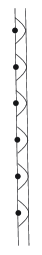
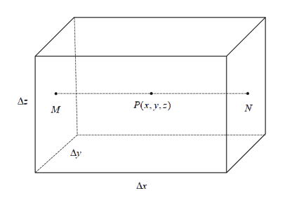
Let us pick some small volume centered at a point , as shown in FIG. 17. At the end of the calculation we shall take the limit .
The number of particles that leave through the right side per unit time of the prism on FIG. 17 (point ) is . If this number is negative, the particles are entering (not leaving) into the prism from the right side. The number of particles that leave through the left side of the prism per unit time on FIG. 17 (point ) is equal to . The total number of particles leaving the prism per unit time through the left and right side of the prism is then:
| (148) |
In the last line we divided and multiplied by and used the fact that for some arbitrary function we have that:
| (149) |
We also add up and for the particles leaving the other sides and then the total number of particles, leaving the prism per unit time is:
| (150) |
Here we have used that . Taking the limit as well as , we obtain the number of particles leaving the volume
| (151) |
On the other hand, the particles that left the volume lead to decrease of its density:
| (152) |
From Eqs. (151) and (152) we derive:
| (153) |
If we divide this equation by and if we take into account that , we finally derive the continuity equation:
| (154) |
XI Acknowledgment
This research did not receive any specific grant from funding agencies in the public, commercial, or not-for-profit sectors.
XII Data Availability Statement
The author confirm that the data supporting the findings of this study are available within the article and/or its supplementary materials.
References
- (1) D. J. Griffiths, Introduction to Quantum Mechanics, Cambridge University Press; 3rd edition (2018)
- (2) C. Cohen-Tanndoudji, Quantum Mechanics, Volume 1: Basic Concepts, Tools, and Applications, Wiley, 2nd edition (2019)
- (3) D. Bohm, Quantum Theory, Dover Publications, Revised Edition (1989)
- (4) A. Messiah, Quantum Mechanics, Dover Publications (2014)
- (5) W. Greiner, D. A. Bromley, Quantum Mechanics: An Introduction, Springer (2001)
- (6) P. A. M. Dirac, Principles of Quantum Mechanics, Oxford University Press, 4th Edition (1959)
- (7) L.D. Landau, and L. M. Lifshitz, Quantum Mechanics (non-relativistic theory): Course of Theoretical Physics, Volume 3, Butterworth-Heinemann, Third Edition (1981)
- (8) A. Sommerfeld, Lectures on Theoretical Physics: Optics, Academic Press (1964)
- (9) M. Born, and E. Wolf, Principles of Optics: Electromagnetic Theory of Propagation, Interference and Diffraction of Light, Cambridge University Press, 7th Edition (19999)
- (10) E. T. Whittaker, A History of the Theories of Aether and Electricity: Two Volumes Bound as One (Dover Publications, 1989)
- (11) M. L. Boas, Mathematical Methods in the Physical Sciences, Wiley, 3rd edition (2005)
- (12) J. Nearing, Mathematical Tool for Physics, Dover Publications (2010)
- (13) T. Maudlin, Philosophy of Physics: Quantum Theory, Princeton University Press (2019)
- (14) S. Frabboni, et al. From measuring electron charge to exploring particle-wave duality: A new didactic experimental approach, Am. J. Phys. 75, 1053 (2007)
- (15) S. Frabboni, et al. Nanofabrication and the realization of Feynman’s two-slit experiment, Appl. Phys. Lett. 93, 073108
- (16) D. Bohm, A Suggested Interpretation of the Quantum Theory in Terms of ”Hidden” Variables. I, Phys. Rev. 85, 166 (1952)
- (17) D.Bohm, and B. J. Hiley, The Undivided Universe, Routledge; 1st Edition (1995)
- (18) T. Norsen, Foundations of Quantum Mechanics: An Exploration of the Physical Meaning of Quantum Theory (Undergraduate Lecture Notes in Physics), Springer (2017)
- (19) A. Sommerfeld, Lectures on Theoretical Physics: Mechanics, Academic Press, First Edition (1964)