Connecting Lyman-$\alpha$ and ionizing photon escape in the Sunburst Arc

Abstract

We investigate the Lyman-$\alpha$ (Ly$\alpha$) and Lyman continuum (LyC) properties of the Sunburst Arc, a $z=2.37$ gravitationally lensed galaxy with a multiply-imaged, compact region leaking LyC and a triple-peaked Ly$\alpha$ profile indicating direct Ly$\alpha$ escape. Non-LyC-leaking regions show a redshifted Ly$\alpha$ peak, a redshifted and central Ly$\alpha$ peak, or a triple-peaked Ly$\alpha$ profile. We measure the properties of the Ly$\alpha$ profile from different regions of the galaxy using $R\sim 5000$ Magellan/MagE spectra. We compare the Ly$\alpha$ spectral properties to LyC and narrowband Ly$\alpha$ maps from Hubble Space Telescope (HST) imaging to explore the subgalactic Ly$\alpha-$LyC connection. We find strong correlations (Pearson correlation coefficient $r>0.6$) between the LyC escape fraction ($f_{\rm esc}^{\rm LyC}$) and Ly$\alpha$ (1) peak separation $v_{\rm{sep}}$, (2) ratio of the minimum flux density between the redshifted and blueshifted Ly$\alpha$ peaks to continuum flux density $f_{\rm{min}}/f_{\rm{cont}}$, and (3) equivalent width. We favor a complex H I geometry to explain the Ly$\alpha$ profiles from non-LyC-leaking regions and suggest two H I geometries that could diffuse and/or rescatter the central Ly$\alpha$ peak from the LyC-leaking region into our sightline across transverse distances of several hundred parsecs. Our results emphasize the complexity of Ly$\alpha$ radiative transfer and its sensitivity to the anisotropies of H I gas on subgalactic scales. Large differences in the physical scales on which we observe spatially variable direct escape Ly$\alpha$, blueshifted Ly$\alpha$, and escaping LyC photons in the Sunburst Arc underscore the importance of resolving the physical scales that govern Ly$\alpha$ and LyC escape.

1 Introduction

Following the formation of the first stars and galaxies, the universe experienced a phase transition during an era known as the Epoch of Reionization (EoR) ($z\sim 6-10$). Prior to this, protons and electrons sufficiently cooled after the hot Big Bang to recombine ($z\sim 1100$; the Epoch of Recombination) into neutral hydrogen (H I). As the earliest generations of ionizing sources formed, they reionized this neutral gas.

How the universe reionized remains an outstanding problem of modern astronomy. The two most likely sources of the ionizing radiation (called the Lyman continuum (LyC), with $\lambda<912$ Å) are star-forming galaxies and active galactic nuclei (AGN). A drastic reduction in the AGN number density at $z>6$ (Masters et al., 2012; Palanque-Delabrouille et al., 2013) might suggest AGN contribute $<10\%$ (but very likely $<30\%$) of the reionization ‘budget’ (Masters et al., 2012; Ricci et al., 2017), but JWST’s discovery of a faint AGN population during and shortly after reionization (Kocevski et al., 2023; Dayal et al., 2024) could challenge this. Other authors have constructed AGN-dominated scenarios consistent with multiple observational constraints (Madau & Haardt, 2015), so the role of AGN in reionization is still controversial.

If star-forming galaxies dominated the reionization of the universe, LyC photons from ionizing sources in star-forming galaxies must have escaped their host galaxy somehow. However, direct observations of the fraction of LyC which escapes galaxies ($f_{\text{esc}}^{\text{LyC}}$) become increasingly difficult at $z>2$, and nearly impossible at $z>4$ (Inoue et al., 2014). This is because the intergalactic medium (IGM) becomes increasingly neutral—and therefore increasingly opaque to LyC photons—as we look back beyond $z\sim 2$.

Additionally, various cosmological hydrodynamical simulations disagree on how different sources contributed to reionization and on the dependence of $f_{\text{esc}}^{\text{LyC}}$ on important properties like galaxy mass and redshift (Gnedin et al., 2008; Ma et al., 2015; Sharma et al., 2016; Kannan et al., 2022). The dilemma becomes further complicated because the observed timescale of reionization (hundreds of Myr; e.g., Planck Collaboration et al. (2016)) is shorter than expected if the galaxies that caused reionization had similar $f_{\rm{esc}}^{\rm{LyC}}$ to local galaxies. This discrepancy suggests the LyC production and escape properties measured in local galaxies do not fully describe the processes that drove reionization. If AGN do not dominate reionization, then to satisfy the reionization budget, $\gtrsim 10-20\,\%$ of LyC must escape from source galaxies (Bolton & Haehnelt, 2007; Ouchi et al., 2009; Kuhlen & Faucher-Giguère, 2012; Robertson et al., 2013, 2015; Mitra et al., 2015; Bouwens et al., 2015; Khaire et al., 2016; Price et al., 2016). But LyC surveys consistently find typical escape fractions $\lesssim 10\%$ (Vanzella et al., 2010; Sandberg et al., 2015; Grazian et al., 2016, 2017; Guaita et al., 2016; Rutkowski et al., 2016, 2017; Vasei et al., 2016). Although JWST has revealed that some galaxies produce ionizing photons much more efficiently than anticipated (e.g., Atek et al. (2023); Endsley et al. (2024)), which would permit reionization scenarios with lower typical escape fractions, it is unclear if these discrepant galaxies are sufficiently numerous. For a complete review of the current understanding of reionization and JWST’s expected impact, see Robertson (2022).

One strategy to identify LyC production and escape methods is to observe post-reionization galaxies believed to be good analogues to reionization galaxies (Izotov et al., 2011, 2016a, 2017a, 2017b, 2018b, 2019a, 2019b, 2021a; Steidel et al., 2018; Fletcher et al., 2019; Flury et al., 2022a, b; Pahl et al., 2022; Schaerer et al., 2022). Targets at $z\lesssim 4$ avoid the excessive IGM attenuation seen at higher redshift (though it is often still nontrivial), such that rest-LyC radiation is accessible with ultraviolet (UV) or optical filters on ground- and space-based instruments. The primary goal of observing later analogues to reionization galaxies is to link LyC escape to UV diagnostics of a galaxy’s interstellar medium (ISM) and stellar populations, which together strongly regulate the production and escape of LyC photons. Connecting UV diagnostics and LyC is vital because the non-ionizing UV to rest-optical is the wavelength band JWST (and soon the generation of extremely large telescopes) directly accesses from reionization galaxies (Williams et al., 2022; Bunker et al., 2023; Lin et al., 2023; Mascia et al., 2023). The relations between UV diagnostics and $f_{\text{esc}}^{\text{LyC}}$ established in lower-redshift analogues can then constrain $f_{\text{esc}}^{\text{LyC}}$ for reionization galaxies and the primary escape methods of LyC photons.

The overarching strategy to find analogues to reionization galaxies is to preselect LyC-leaking candidates based on indirect tracers of LyC escape (e.g., the [O III] 4959, 5007 Å / [O II] 3727, 3729 Å ratio O32 or Ly$\alpha$ peak separation $v_{\text{sep}}$). In this fashion, many post-reionization LyC leakers have been identified (Bergvall et al., 2006; Leitet et al., 2011, 2013; Borthakur et al., 2014; Mostardi et al., 2015; de Barros et al., 2016; Izotov et al., 2016b, c, 2018a, 2018c, 2020, 2021b, 2022; Leitherer et al., 2016; Shapley et al., 2016; Bian et al., 2017; Puschnig et al., 2017; Steidel et al., 2018; Vanzella et al., 2018; Fletcher et al., 2019; Ji et al., 2020; Saha et al., 2020; Jones et al., 2021; Malkan & Malkan, 2021; Marques-Chaves et al., 2021, 2022; Saxena et al., 2022; Flury et al., 2022a, b), though generally with insufficient spatial resolution to resolve the small scales (down to tens of parsecs and less) expected to dictate LyC escape. Notably, Rivera-Thorsen et al. (2022) conducted a bottom-up search for LyC sources selected solely by their LyC emission in archival HST imaging that suggested the preselection criteria normally imposed in LyC emitter searches may miss nontrivial contributors to the ionizing background.

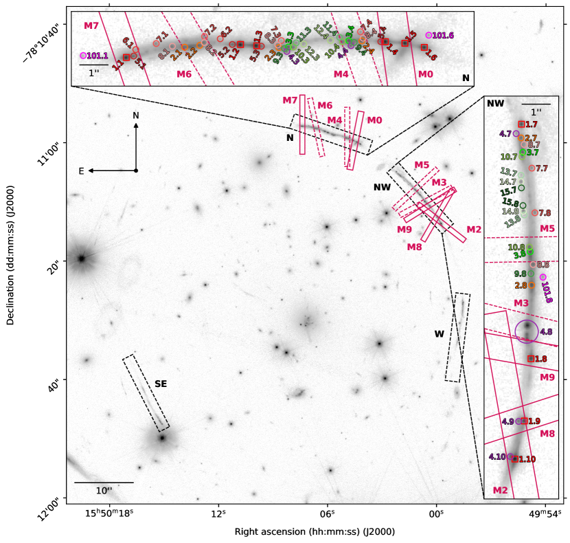
Figure 1: HST/WFC3 F606W imaging of the Sunburst Arc from GO-15377 (PI: M. Bayliss). Black dashed rectangles on the main image mark the main arc segments, labeled as in Sharon et al. (2022). The inset panels enlarge the two largest arcs, which are the focus of spectroscopic MagE data presented in this work (Table 1). The MagE apertures appear as magenta rectangles, where solid apertures cover images of the LyC-leaking region, and dashed apertures do not. In the inset panels, circles (except for squares for the LyC-leaking region) mark images of different source plane regions of the Sunburst Arc, as labeled and colored in the lens model of Sharon et al. (2022).

This search for tracers of LyC escape, spurred by the simultaneous necessity to understand the process of reionization and inability to directly observe LyC from reionization, makes the galaxy PSZ1-ARC G311.6602-18.4624—nicknamed the Sunburst Arc by Rivera-Thorsen et al. (2017)—a compelling target to study LyC escape. The Sunburst Arc is a strongly lensed (magnifications between $\sim 10-100\times$ (Rivera-Thorsen et al., 2019; Pignataro et al., 2021; Sharon et al., 2022)) galaxy arc at redshift $z\approx 2.37$. Discovered by Dahle et al. 2016, the Sunburst Arc has garnered great interest because of (1) its high LyC escape fraction (Rivera-Thorsen et al., 2017, 2019; Vanzella et al., 2021), (2) the unique mode of LyC escape implied by its Ly$\alpha$ emission, and (3) the advantages offered by the strong lensing in studying LyC escape. The foreground galaxy cluster PSZ1 G311.65-18.48 at $z\approx 0.44$ lenses the Sunburst Arc into 12 full or partial images of the galaxy that show at least 54 individual features in total (Pignataro et al., 2021; Sharon et al., 2022). Some of these images could represent individual star clusters with radius as small as $\lesssim 20$ pc (Vanzella et al., 2021). A compact LyC-emitting region appears at least 12 times (Rivera-Thorsen et al., 2019), and may be less than 10 pc across (Mestric et al., 2023).

Previous studies strongly disfavor the presence of an AGN in the Sunburst Arc (Rivera-Thorsen et al., 2019; Mainali et al., 2022). Instead, past work favors young, massive stars produced in a recent burst of star formation as responsible for the observed LyC photons, mainly evidenced by the P-Cygni wind profiles, high-velocity and highly ionized galactic outflows, and compact regions with extremely blue UV slopes characteristic of hot, young stellar populations (Rivera-Thorsen et al., 2017, 2019; Chisholm et al., 2019; Mainali et al., 2022; Mestric et al., 2023; Pascale et al., 2023; Kim et al., 2023). Together, the excellent spatial resolution in the source plane, multiple lines of sight into the galaxy, high signal-to-noise, and young stellar populations make the Sunburst Arc an ideal target to understand how LyC photons may have escaped from earlier star-forming galaxies during reionization.

Table 1: MagE observation log and magnifications

Slit	Position	Width	Date	Exp. time	FWHM	R	$\mu$
	[(hh:mm:ss, dd:mm:ss)]	[$\arcsec$]		[ks]	[$\arcsec$]
M5	(15:50:01.1649, -78:11:07.822)	0.85	2018 Apr 22	13.5	$0.97$	5500 $\pm$ 400	$51^{+5}_{-10}$
M4	(15:50:04.9279, -78:10:59.032)	0.85	2018 Apr 21	7.2	$0.71$	5400 $\pm$ 300	$14.6^{+0.8}_{-3}$
M6	(15:50:06.6389, -78:10:57.412)	0.85	2018 Apr 22, 23	12.9	$0.76$	5300 $\pm$ 300	$147^{+5}_{-20}$
M3	(15:50:00.6009, -78:11:09.912)	0.85	2018 Apr 21	12	$0.70$	5500 $\pm$ 400	$36^{+4}_{-5}$
M0	(15:50:04.4759, -78:10:59.652)	1	2017 May 24	13.5	$1.34$	4700 $\pm$ 200	$10^{+10}_{-7}$
M2	(15:49:59.7480, -78:11:13.482)	0.85	2018 Apr 21, 23	8.1	$0.77$	5300 $\pm$ 300	$32^{+6}_{-3}$
M7	(15:50:07.3959, -78:10:56.962)	0.85	2018 Aug 11, 12	14.4	$0.73$	5200 $\pm$ 200	$35^{+3}_{-6}$
M8	(15:49:59.9499, -78:11:12.242)	0.85	2018 Aug 10, 11, 12	14.4	$0.70$	5200 $\pm$ 300	$29^{+6}_{-3}$
M9	(15:50:00.3719, -78:11:10.512)	0.85	2018 Apr 23	13.5	$0.68$	5500 $\pm$ 400	$31^{+4}_{-3}$

Note. — From left to right: slit label, position in (right ascension (hh:mm:ss), declination (dd:mm:ss)) (J2000), slit width in arcseconds, UT observation date, total exposure time in kiloseconds, individual exposure time-weighted average of the seeing conditions in arcseconds, median spectral resolution (R) as determined by the widths of night sky lines, and average magnification ($\mu$), as calculated using the lens model of Sharon et al. (2022).

A promising tool to investigate LyC escape is a source’s Lyman-$\alpha$ (Ly$\alpha$) emission (see, e.g., Verhamme et al. (2015)). Ly$\alpha$ photons primarily originate from recombining H II ions and free electrons in H II regions around massive OB stars producing copious LyC photons, implying that Ly$\alpha$ and LyC photons begin their journeys not far from each other. As a resonant emission line of H I, Ly$\alpha$ photons interact strongly with the same gas that attenuates LyC from sources within a galaxy (stronger, in fact, than LyC; Draine (2011)). So, the intricate radiative transfer of Ly$\alpha$ (for a review, see, e.g., Dijkstra (2017)) encodes complex information about the H I that LyC photons must navigate to escape the galaxy. Though H I governs the paths of Ly$\alpha$ and LyC photons, both are sensitive to significantly different column densities (e.g., for $\tau=1$, $\log_{10}(N_{\text{HI}}\,[\textrm{cm}^{-2}])\sim 13.8$ and $\log_{10}(N_{\text{HI}}\,[\textrm{cm}^{-2}])\sim 17$ for Ly$\alpha$ and LyC photons, respectively). The different column density sensitivities, coupled with the resonant nature of Ly$\alpha$, necessitates different interpretation approaches for Ly$\alpha$ and LyC signatures. LyC photons travel along a sightline until destroyed by intervening material (H I or dust), but H I can rescatter Ly$\alpha$ photons many times (provided dust does not destroy those Ly$\alpha$ photons). And crucially, unlike Ly$\alpha$ photons, LyC photons are not strongly sensitive to the kinematics of H I. This means Ly$\alpha$ photons may not actually follow the observed sightlines, and could have originated from a different physical region than observed. So, Ly$\alpha$ properties do not necessarily correspond with the areas that they appear to come from, and may appear diffused to a much larger area than the progenitor H II regions (e.g., Östlin et al. (2014); Hayes et al. (2014); Rivera-Thorsen et al. (2015); Herenz et al. (2016); Bridge et al. (2018); Rasekh et al. (2022); Melinder et al. (2023)).

Because of the complex connection between the regulation of Ly$\alpha$ and LyC photon escape, one of the Sunburst Arc’s most remarkable features is its triple-peaked Ly$\alpha$ profile, which we investigate in this work. Rivera-Thorsen et al. (2017) first reported this feature, originally predicted by Behrens et al. (2014), and seldom observed in other galaxies (Izotov et al., 2018c; Vanzella et al., 2018, 2020a). As we present, with one exception, all observations of triple-peaked Ly$\alpha$ profiles in the Sunburst Arc seem associated with the LyC-leaking region. So, this unique Ly$\alpha$ profile may be connected to LyC escape. Observations and radiative transfer models of Ly$\alpha$ often explain this unique profile with a perforated covering shell of H I that permits direct escape of Ly$\alpha$ and LyC photons through one or several holes, but otherwise scatters (attenuates) Ly$\alpha$ (LyC) photons (Behrens et al., 2014; Verhamme et al., 2015; Rivera-Thorsen et al., 2015, 2017).

In this work, we analyze rest-UV and rest-optical observations of the Sunburst Arc from slit spectroscopy with Magellan/MagE (§ 2.1) and archival multi-filter imaging with HST (§ 2.2). We specifically study the Ly$\alpha$ properties of regions of the galaxy and their $f_{\text{esc}}^{\text{LyC}}$ to build a physical picture of how Ly$\alpha$ and LyC photons escape the galaxy. To accomplish this, we fitted the Ly$\alpha$ spectra (§ 3.5) and calculated estimates of $f_{\rm{esc}}^{\rm{LyC}}$ in the spectroscopic apertures from the HST imaging (§ 3.4). We compare common Ly$\alpha$ parameters to determine their mutual dependence and relation to LyC escape (§ 4). In § 5 we present several hypotheses to explain the spatial variation of the Ly$\alpha$ velocity profiles and their connection to LyC escape, ultimately favoring unique source plane H I morphologies as causative mechanisms for the observed Ly$\alpha$ and LyC signatures. We conclude in § 6 with implications for future Ly$\alpha$ and LyC observations in lensed galaxies.

Throughout this work, we assume a flat $\Lambda$CDM cosmology with $H_{0}=70$ km s^-1 Mpc^-1, $\Omega_{m}=0.3$, and $\Omega_{\Lambda}=0.7$.

2 Observations

This work used rest-frame Ly$\alpha$ spectra from Magellan/MagE (§ 2.1) as well as HST imaging of the rest-frame Ly$\alpha$ (HST/WFC3 F410M), LyC (HST/WFC3 F275W), near-UV continuum (HST/ACS F814W, WFC3 F390W, F555W, F606W) and rest-frame optical narrowband (HST/WFC3 F128N, F153M) (§ 2.2). See Tables 1 and 2 for descriptions of the respective Magellan and HST observations.

2.1 Magellan spectroscopy

We observed 9 locations on the 2 largest arcs of the Sunburst Arc (Figure 1) in the observed-frame optical ($\sim 3200-8500$ Å) wavelengths with the Magellan Echellette (MagE) spectrograph (Marshall et al., 2008) mounted on the Magellan-I Baade Telescope (6.5m) at the Las Campanas Observatory in Chile. These spectra cover the rest-UV ($\sim 950-2500$ Å, including Ly$\alpha$) at the redshift of the Sunburst Arc. Apart from slit M0, which predated the acquisition of HST imaging, we compared the MagE slit viewing camera to HST images to precisely position the slits along the arc. M0 simply targeted the brightest part of the arc as measured in discovery imaging from the European Southern Observatory’s New Technology Telescope (Dahle et al., 2016). Of the 9 apertures, the HST imaging reveals that 5 apertures target images of the LyC-leaking region and 4 do not. One slit (M3) covers an unusual, highly magnified object previously discussed by Vanzella et al. (2020b), Diego et al. (2022), Sharon et al. (2022), Pascale & Dai (2024), and Choe et al. (2024) (image 4.8 in Figures 1, 4), favored to be a supernova by Vanzella et al. (2020b) and later a luminous blue variable (LBV) star in outburst by Diego et al. (2022). Sharon et al. (2022) presented evidence the unusual source is not a transient event, and is likely due to an unusual lensing configuration, as suggested by Diego et al. (2022). Table 1 summarizes the MagE pointings. Rigby et al. (in prep.) will present the full observation log for each pointing. The MagE data were reduced following the same methods as described in Rigby et al. (2018). Slits M0 and M3 and two conglomerate stacked spectra are the only previously published portions of these MagE observations (first published in Rivera-Thorsen et al. (2017), Choe et al. (2024), and Mainali et al. (2022), respectively). The reduction procedure of the new data presented here is identical to the reduction for slit M0 published in Rivera-Thorsen et al. (2017). The MagE observations of Ly$\alpha$ appear in Figure 2.

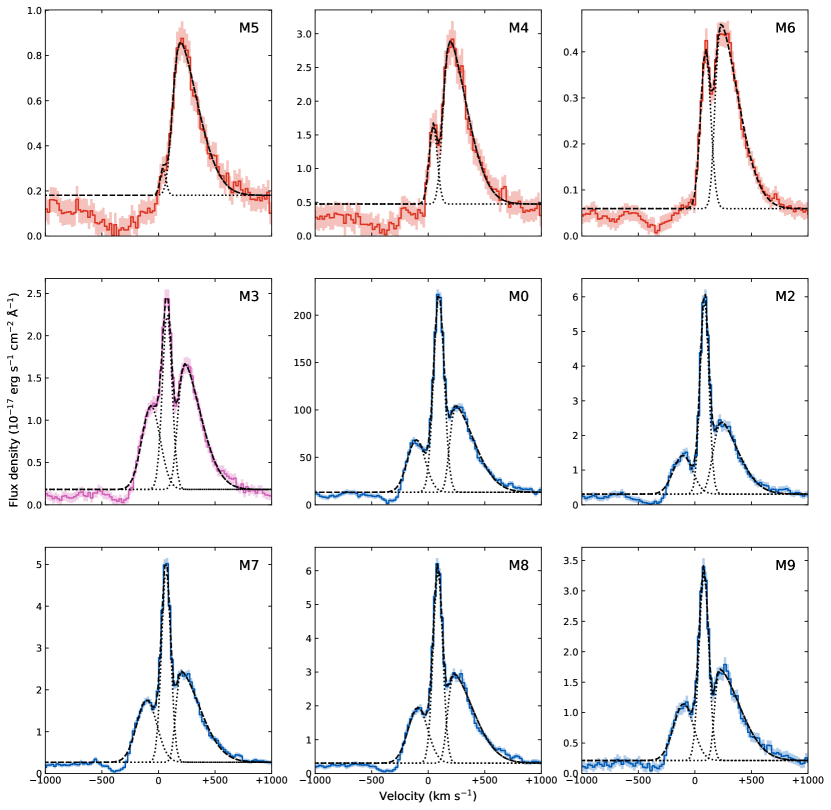
Figure 2: The magnification-corrected, rest-frame Ly$\alpha$ profiles, ordered from left to right, then top to bottom, first by increasing central Ly$\alpha$ peak strength relative to the redshifted Ly$\alpha$ peak in the non-LyC-leaking apertures, then the LyC-leaking apertures by the numeric order of their slit identifier. Those in red (top row) are non-LyC-leaking apertures (slits M5, M4, and M6), in pink (slit M3) is a non-LyC-leaking aperture targeting a highly magnified, exotic object (see § 5.1 for more details), and in blue are the LyC-leaking apertures (slits M0, M2, M7, M8, and M9). The dashed black lines represent the overall fits and dotted black lines represent the individual Ly$\alpha$ peak fits, based on the median best-fit parameters from the fitting described in § 3.5.4. The shaded region represents the $2\sigma$ uncertainties of the flux densities. The observations clearly show a significant variety of Ly$\alpha$ profiles in the Sunburst Arc. Slit M0 has a much larger flux density scale due to poor observing conditions that prevented an accurate fluxing (see Table 1 for more details about the observation).

2.2 HST imaging

We adopted some HST data used in this work as reduced and presented in other works: the ACS F814W and WFC3 F390W, F410M, F555W, and F606W observations in Sharon et al. (2022), and the WFC3 F128N, F153M observations in Kim et al. (2023).

We analyzed new, ultra deep rest-LyC images, adding 26 additional orbits of F275W (GO-15949, PI: M. Gladders) to the 3 orbits of F275W previously presented in Rivera-Thorsen et al. (2019) (GO-15418, PI: H. Dahle), resulting in a total of 29 orbits (86.9 ks) of integration time. The new F275W observations were structured in visits of typically three orbits, with two full-orbit integrations to minimize effects of charge transfer inefficiency, and two half-orbit integrations, providing a total of four frames to ensure good cosmic ray rejection and point spread function (PSF) reconstruction in each visit. Individual processed frames were taken from the Mikulski Archive for Space Telescopes and stacked using the tools in the DrizzlePac package. The final stacked image was astrometrically referenced to the F606W imaging, with a pixel scale of 0.03″ pixel^-1 and a 0.6 pixel Gaussian drizzle drop size. The deeper exposures achieve a 5$\sigma$ depth of $m_{\rm{AB}}\approx 29.9$ (compared to the corresponding 5$\sigma$ depth of $m_{\rm{AB}}\approx 28$ from the shallower exposures in Rivera-Thorsen et al. (2019)) but do not reveal any new LyC-leaking images or LyC morphology than presented in Rivera-Thorsen et al. (2019). Figure 4 shows the new LyC maps of the two main segments of the Sunburst Arc targeted by this work’s MagE slit apertures. Table 2 summarizes the HST observations used in this work.

All the HST data used in this paper can be found in MAST: https://dx.doi.org/10.17909/t87g-a816 (catalog https://dx.doi.org/10.17909/t87g-a816).

Table 2: HST observations

Camera	Filter	$\lambda_{\rm pivot}$	Width	$t_{\rm{exp}}$	Purpose	Program
		[Å]	[Å]	[s]
ACS	WFC/F814W	8333	2511	5280	$f_{\rm{esc}}^{\rm{LyC}}$, SED fit	GO-15101
WFC3	IR/F128N	12832	159	16818	SED fit	GO-15949
	IR/F153M	15322	685	5612	SED fit	GO-15949
	UVIS/F275W	2710	405	5413	$f_{\rm{esc}}^{\rm{LyC}}$	GO-15418
	UVIS/F275W	—	—	81489	$f_{\rm{esc}}^{\rm{LyC}}$	GO-15949
	UVIS/F390W	3924	894	3922	Ly$\alpha$ off-band	GO-15949
	UVIS/F410M	4109	172	13285	Ly$\alpha$ on-band	GO-15101
	UVIS/F555W	5308	1565	5616	Ly$\alpha$ off-band, SED fit	GO-15101
	UVIS/F606W	5889	2189	5830	SED fit	GO-15377

Note. — HST observations used in this work. From left to right: HST instrument, filter, pivot wavelength of filter in angstroms, filter width in angstroms, exposure time in seconds, purpose for this work, and program ID.

3 Data Analysis

3.1 Redshifts

We adopted the spectroscopic redshifts presented by Mainali et al. (2022) (Table 1 therein), measured from the narrow component of the strong rest-optical nebular emission line [O III] 5007 Å of the MagE targets, captured with the Folded-port InfraRed Echellette (FIRE) (Simcoe et al., 2013) mounted on the Magellan-I Baade Telescope. See Figure 1 in Mainali et al. (2022) for a comparison between the FIRE and MagE pointings (all the MagE pointings discussed in this paper have overlapping FIRE pointings) and their Section 3.3 for a description of how they computed the redshifts of the targeted regions of the galaxy. We did not adopt a single redshift for the galaxy because it is critical to accurately place each MagE spectrum into the rest frame while, e.g., stacking the spectra, or accurately determining peculiar velocities.

3.2 Stacking spectra

Rivera-Thorsen et al. (2019) identified the LyC-leaking images in the Sunburst Arc as a compact, star-forming region, which Mainali et al. (2022) used to justify stacking the MagE spectra of the LyC-leaking and non-LyC-leaking images to compare the two sets of regions. We repeated this stacking (labeling the stacked LyC-leaking and non-LyC-leaking spectra as L and NL, respectively), but excluded slit M0 from the LyC-leaking stack due to the poor observing conditions (see Table 1) that prevented an accurate fluxing, and the presence of a foreground galaxy in the aperture (see the diffuse emission southeast of image 1.5 in Figure 1), and also excluded slit M3 from either stack, as it includes a bright image of an extremely magnified area of the galaxy (Diego et al., 2022; Sharon et al., 2022) that may not be representative of the broader region it is embedded in (see § 5.1 for more details). To create the stacks, we normalized the individual spectra used to create a stack by their median flux density between $1267-1276$ Å in the rest frame, interpolated them to a common set of identically-sized wavelength bins, and then averaged their flux densities at each bin. Figure 3 shows the stacked Ly$\alpha$ spectra.

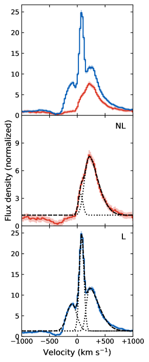
Figure 3: Ly$\alpha$ profiles of the stacked LyC-leaking and non-LyC-leaking MagE slit apertures with fits. Top: Ly$\alpha$ profiles of the stacked LyC leaker (above in blue) and non-LyC-leaking regions (below in red). The shaded regions indicate the 3$\sigma$ uncertainty of the flux density. Center: Stacked Ly$\alpha$ profile of the non-LyC-leaking apertures with the total fit in dashed black and individual peak fits in dotted black. Bottom: Stacked LyC leaker Ly$\alpha$ profile with the total fit in dashed black and individual peak fits in dotted black.

3.3 Creating narrowband Ly$\alpha$ maps

To supplement the spectroscopic Ly$\alpha$ data with spatial Ly$\alpha$ information, we created Ly$\alpha$ images by estimating the contribution of Ly$\alpha$ to the emission observed in the F410M filter using an approach similar to that described in Section 2.5 of Kim et al. (2023). We fit SED models to the integrated F153M, F128N, F814W, F606W, and F555W photometry of four images of the multiply-imaged source galaxy, which include flux from image families 3, 4, 8, 9, and 10 (using the nomenclature of Sharon et al., 2022). These four fits should produce nearly identical SEDs because they are fit to different lensed images of the same source. Fitting four different SEDs provides a direct estimate of any systematic variations caused by differential magnification between the different emission clumps in the lensed galaxy.

We used prospector, an MCMC-based stellar population synthesis and parameter inference framework (Conroy & Gunn, 2010; Foreman-Mackey et al., 2013; Johnson et al., 2021) to fit SED models with a delayed-$\tau$ (with age and $e$-folding time of SFR as free parameters) + constant star formation model, and also fitted for stellar mass, dust attenuation (using the Calzetti attenuation model), and the gas ionization parameter log $U$. We used a fixed value for stellar metallicity ($\rm{log}(Z/Z_{\odot})=-0.33$, informed by spectroscopy), and a Kroupa initial mass function (Kroupa, 2001), and evaluated nebular continuum and line emission via the CLOUDY component of the embedded Flexible Stellar Population Synthesis (FSPS; Johnson et al. 2022) framework (see Byler et al. (2017) for details). We took the stellar and nebular continuum from the highest posterior probability SED model as a proxy for the true continuum. The SEDs and filter transmission curves (except F606W and F814W) appear in Figure 7 of Kim et al. (2023). We corrected the SEDs for Milky Way dust extinction according to the 3-dimensional interstellar dust extinction map of Green et al. (2015).

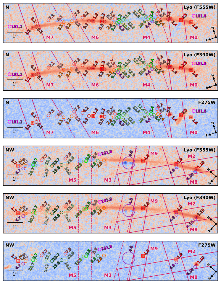
Figure 4: The rest-LyC (F275W) and Ly$\alpha$ maps of the north (N) and northwest (NW) segments of the Sunburst Arc, with the MagE slit apertures overlaid in magenta and the identified images of the Sunburst Arc marked and labeled following the color and naming scheme of Sharon et al. (2022). Boxes mark images of the LyC-leaking region and circles mark all other images. The filter in parentheses in the Ly$\alpha$ map labels indicates the filter used to estimate the background continuum contribution to the count rate of F410M, which includes the Ly$\alpha$ line.

These SEDs did not model attenuation from the Ly$\alpha$ forest, which may cause an over-subtraction of the continuum. To test if this was an issue, we normalized each SED at an observed wavelength of 1 $\mu$m and compared the SED count rates in the on-band (on-Ly$\alpha$) F410M filter with the count rates predicted for F410M from the stacked MagE LyC-leaking and non-LyC-leaking spectra after masking out Ly$\alpha$ and other emission lines, and convolving the data with a boxcar kernel. We found no significant difference between the predicted F410M continuum count rates from the SED fitting and the Ly$\alpha$-removed, scaled MagE spectra.

We calculated the Ly$\alpha$ emission as Ly$\alpha$ flux equal to on-band flux minus off-band flux $\times$ a scaling factor. We estimated the scaling factor as the mean of the individual scaling factors of the different continuum models described above. We used the standard deviation of the individual scaling factors of the models as an estimate of the systematic uncertainty in the scaling factor. We estimated the statistical uncertainty in the continuum subtraction from regions of empty sky in the data. We made two maps: one with F390W as the off-band filter—which samples continuum closer to Ly$\alpha$ but includes Ly$\alpha$ and Ly$\alpha$ forest-attenuated continuum—and one with F555W as the off-band filter—which samples continuum farther from Ly$\alpha$. Figure 4 shows the Ly$\alpha$ maps of the two segments of the Sunburst Arc for both off-band filter choices. We report uncertainties of measurements made from the Ly$\alpha$ maps with the combined systematic and statistical uncertainties.

3.4 Measuring $f_{\text{esc}}^{\text{LyC}}$

Rivera-Thorsen et al. (2019) previously computed $f_{\text{esc}}^{\text{LyC}}$ for the images of the LyC-leaking region, and more recently, Pascale et al. (2023) have indirectly estimated the LyC-leaking region’s $f_{\text{esc}}^{\text{LyC}}$ from the observed nebular continuum and nebular line strengths. The MagE apertures include 5 slits that cover 6 of the LyC-leaking images investigated in Rivera-Thorsen et al. (2019), but also 4 slits that only cover images of the galaxy that do not leak LyC (Figure 1). We computed the IGM-unattenuated, absolute LyC escape fraction $f_{\text{esc}}^{\text{LyC}}$ within each MagE aperture. We adapted the method Rivera-Thorsen et al. (2019) used to calculate the apparent, relative LyC escape fraction, summarized in their Equation S3. Briefly, they used the non-ionizing rest-UV continuum F814W observations (unaffected by H I absorption) in tandem with theoretical, intrinsic Starburst99 (Leitherer et al., 1999) spectra to compute the expected flux in F275W if the sightline were completely transparent to LyC. To instead compute the IGM-unattenuated, absolute LyC escape fractions, we shifted the IGM transmission factor in their Equation S3 to the opposite side of the equation and used dust-extincted Starburst99 spectra instead of the intrinsic Starburst99 spectra.

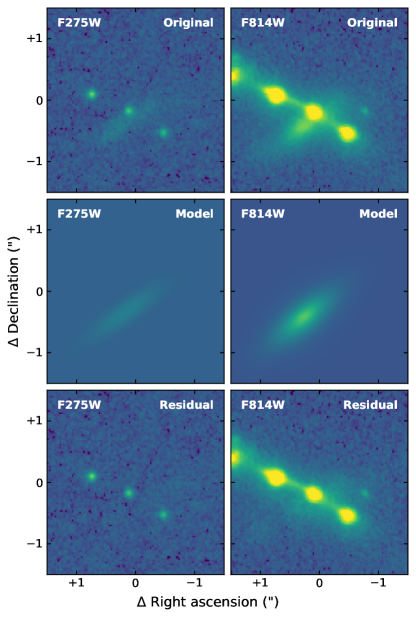
Figure 5: Results of using Galfit to remove a foreground galaxy over an image of the LyC leaker (image 1.5 in Figure 1) from the F275W and F814W images. Each column uses the same color map with a cube root scale, with minima (maxima) of the masked median of the cutout minus $2$ $\times$ (plus $100$ $\times$) the standard deviation of the source-masked cutout. The Galfit models have a flat background of 0.

To prepare the F275W and F814W images to measure the necessary photometry, we (1) removed a foreground interloping galaxy, and (2) subtracted the background level from the images. The foreground galaxy is bright in F275W, contaminating slit M0 (see the diffuse emission SE of image 1.5 in Figure 1). We subtracted the galaxy from the F275W and F814W imaging with the galaxy surface brightness profile modeling software Galfit (Peng et al., 2010). We fitted the galaxy with a single Sérsic profile in both F275W and F814W. We computed PSF models for both bands using in-field stars. The Galfit results appear in Figure 5.

The summed F275W flux in a MagE aperture is sensitive to the background level of the drizzled image (and thus so is $f_{\text{esc}}^{\text{LyC}}$). Background level overestimates will underpredict $f_{\text{esc}}^{\text{LyC}}$, while underestimates will overpredict $f_{\text{esc}}^{\text{LyC}}$. To accurately model the complex background level, we used the Python Photutils package (Bradley et al., 2022). We iterated the background modeling parameters until the F275W flux in the non-LyC-leaking apertures was consistent with minimal flux.

Although these steps make the images ready for photometry measurements, unlike Rivera-Thorsen et al. (2019), this work aims to closely compare LyC escape fractions to spectroscopic properties. The LyC escape fractions are measurable on a much smaller scale than the spectroscopic properties, since the latter are associated with a slit aperture (to compare, Rivera-Thorsen et al. (2019) used square apertures $\sim 0.1\arcsec$ across to measure photometries of images, as opposed to the $0.85\arcsec$ or $1\arcsec$ width of the MagE slit apertures). For this reason, it is important to match the LyC escape fraction measurements to the same physical scales sampled by the ground-based spectra for the most direct comparison between the spectroscopic and photometric properties. To accomplish this, we measured a single LyC escape fraction measurement for each slit aperture by first convolving the background-subtracted HST imaging with a 2-dimensional Gaussian kernel with a full width at half maximum (FWHM) matching the exposure time-weighted average of the observation’s seeing conditions (Table 1), accounting for the airmass of each exposure of each slit aperture (Rigby et al. in prep.). We then measured the F275W and F814W fluxes associated with the LyC escape fraction measurement as the total flux in either filter inside the intersection of masks of the slit aperture and the Sunburst Arc, proceeding with the measured photometry in otherwise the same fashion as Rivera-Thorsen et al. (2019). See Table 3 for the results.

For each slit aperture and each filter, we estimated the uncertainty of each pixel in the images as the standard deviation of the flux densities outside of the arc mask but inside the aperture. We conservatively assumed a constant 10% uncertainty for the Starburst99 stellar continuum fits of each spectrum. We propagated these uncertainties through the calculation of the LyC escape fractions.

Table 3: HST-based properties of the MagE spectra

Slit	$F_{275}$	$F_{814}$	$f_{\rm{esc}}^{\rm{LyC}}$
M5	$20\pm 20$	$14580\pm 70$	$4\pm 5$
M4	$4\pm 20$	$26760\pm 60$	$0.5\pm 3$
M6	$50\pm 20$	$26700\pm 200$	$6\pm 3$
M3	$40\pm 20$	$26680\pm 60$	$5\pm 3$
M0	$290\pm 30$	$32580\pm 80$	$46\pm 4$
M2	$370\pm 30$	$39740\pm 80$	$30\pm 3$
M7	$120\pm 20$	$19680\pm 60$	$22\pm 4$
M8	$100\pm 30$	$12900\pm 70$	$20\pm 5$
M9	$150\pm 30$	$21220\pm 70$	$19\pm 3$

Note. — From left to right: slit label, flux in the HST/WFC3 F275W and HST/ACS F814W filters ($10^{-19}$ erg s^-1 cm^-2), and $f_{\text{esc}}^{\text{LyC}}$ (%), all computed according to § 3.4.

3.5 Measuring Ly$\alpha$ properties

For all the following quantities, we used a Monte Carlo (MC) measurement process of 10,000 iterations with a burn-in simulation of 1,000 iterations to estimate their values, in which we assumed the flux density and flux density uncertainty associated with each wavelength bin of the MagE spectra corresponded respectively to the mean and standard deviation of a Gaussian distribution. In each iteration, we drew a random sample from the Gaussian distributions corresponding to each wavelength bin to create a new mock spectrum that we then used to measure the discussed quantities. In the main text, figures, and tables, for a given measurement’s distribution, we cite the median $M$, and absolute differences between $M$ and the 16th and 84th percentiles $A$ and $B$, respectively, of the Monte Carlo simulation results as $\rm{M}_{-\rm{A}}^{+\rm{B}}$.

In all Ly$\alpha$ profiles, we measured the FWHM of the central and redshifted Ly$\alpha$ peaks (§ 3.5.4), the ratio $f_{\rm{min}}/f_{\rm{cont}}$ (introduced in § 3.5.5), the rest-frame Ly$\alpha$ equivalent width (EW) (§ 3.5.1), and central escape fraction $f_{\rm{cen}}$ (Naidu et al. (2022); introduced later in § 3.5.3). If the Ly$\alpha$ profile also had a blueshifted Ly$\alpha$ peak, we measured its FWHM and the velocity separation between the redshifted and blueshifted Ly$\alpha$ peaks (§ 3.5.4). In non-stacked spectra, we also measured the magnification-corrected Ly$\alpha$ luminosity (§ 3.5.2). Table 4 contains the measurements.

3.5.1 Equivalent width

The equivalent width of an absorption or emission line is a measure of its strength relative to the continuum level. In this work, we choose the convention that emission lines have positive equivalent widths, and vice versa for absorption lines, so that the equivalent width is

$$\text{EW}=-\int_{\lambda_{1}}^{\lambda_{2}}\left(1-\frac{F_{\lambda}}{F_{c}}\right)\,d\lambda.$$ (1)

Here $F_{\lambda}$ is the flux density, $F_{c}$ the continuum flux density, and $\lambda_{1},\lambda_{2}$ are the integration bounds over the spectral feature.

We applied Equation 1 to compute the rest-frame Ly$\alpha$ EW by integrating between $1212-1221$ Å in the rest frame, as in Yang et al. (2017). We sampled the continuum flux density as the median flux density between $1221-1225$ Å in the rest frame.

3.5.2 Luminosity

To compute the Ly$\alpha$ luminosity, we integrated the continuum-subtracted (taking the local continuum as in $\S$ 3.5.1), magnification-corrected flux density between $1212-1221$ Å in the rest frame.

3.5.3 $f_{\text{cen}}$

The central fraction of Ly$\alpha$ flux, $f_{\rm{cen}}$, introduced by Naidu et al. (2022), is

$$f_{\text{cen}}=\frac{\text{Ly\alpha fluxbetween\pm 100\,kms^{-1}}}{\text{Ly\alpha fluxbetween\pm 1000\,kms^{-1}}},$$ (2)

so named because it integrates the flux densities in the specified velocity bands centered on the wavelength of Ly$\alpha$. The numerator, which targets a narrow band about the Ly$\alpha$ wavelength, is sensitive to Ly$\alpha$ photons that have not been rescattered (attenuated) much by H I (dust). But due to the ‘random walk’ nature of a Ly$\alpha$ photon’s radiative transfer, the numerator also includes any Ly$\alpha$ photons that randomly walk back to the central wavelength band after significant reprocessing. If significantly underdense sightlines exist to the areas of Ly$\alpha$ production, Ly$\alpha$ photons escaping through them should appear in the central wavelength band. The denominator captures virtually all Ly$\alpha$ flux. Thus, $f_{\rm{cen}}$ represents the relative strength of minimally scattered Ly$\alpha$ photons compared to the total number of Ly$\alpha$ photons. Naidu et al. (2022) predict that $f_{\rm{cen}}$ should correlate with the LyC escape fraction, since LyC photons must navigate similar obstacles (i.e., H I and dust) to escape a galaxy.

3.5.4 Peak widths and separation

Determining the width and separation of the Ly$\alpha$ peaks depends on the structure of the Ly$\alpha$ profile in question. We organized the spectra into two cases: (i) there is a redshifted, blueshifted, and central Ly$\alpha$ peak, and (ii) there is not a clear blueshifted Ly$\alpha$ peak. This dichotomy implies that all the spectra have central Ly$\alpha$ peaks, even though slit M5 does not clearly show a central Ly$\alpha$ peak. We still include slit M5 in the two-case dichotomy (the latter case) in order to constrain the possibility of a faint, unresolved central Ly$\alpha$ peak. Most (all the LyC-leaking spectra and slit M3) of the spectra fall into case (i), and only some of the non-LyC-leaking spectra occupy case (ii) (slits M4, M5, and M6).

Rivera-Thorsen et al. (2017) previously modeled the central peak as a Gaussian function of the form

$$\Gamma_{\lambda}(v)=\alpha e^{-\frac{1}{2}((v-\mu)/\sigma)^{2}},$$ (3)

where $\alpha$ is its amplitude, $\mu$ its centroid, and $\sigma$ its standard deviation. Other authors (e.g., Mallery et al. 2012, U et al. 2015, Cao et al. 2020) have treated double-peaked Ly$\alpha$ profiles (those with a redshifted and blueshifted Ly$\alpha$ peak) as two skewed Gaussian functions that follow the form

$$\xi_{\lambda}(v)=\Gamma_{\lambda}(v)\left[1+{\rm{erf}}\left(\frac{\omega(v-\mu)}{\sqrt{2}\sigma}\right)\right].$$ (4)

Here $\omega$ is the skewness, which controls how skewed the distribution is, and ${\rm{erf}}(x)$ is the error function, a complex function with complex variable $x$ defined as

$${\rm{erf}}(x)=\frac{2}{\sqrt{\pi}}\int_{0}^{x}e^{-t^{2}}\,dt.$$ (5)

Right-skewed distributions (i.e., a redshifted Ly$\alpha$ peak) have $\omega>0$ and left-skewed distributions (i.e., a blueshifted Ly$\alpha$ peak) have $\omega<0$.

We combined these two approaches by simultaneously fitting the Ly$\alpha$ profiles to a combination of Gaussian and skewed Gaussian functions with the curve_fit() function in the SciPy Python package. We directly measured each peak’s FWHM and the separation between the redshifted and blueshifted Ly$\alpha$ peaks $v_{\rm{sep}}$ from the resulting fit. To determine the intrinsic FWHM of a peak, we assumed the overall FWHM measured from the observed spectrum as Gaussian, and deconvolved it with the assumed Gaussian line spread function of the instrument (${\rm FWHM}=c/R$), randomly sampling the spectral resolution at each iteration of the MC procedure from a Gaussian distribution described by the spectral resolutions in Table 1. We determined the spectral resolution of the stacked spectra by averaging the spectral resolutions of their composite spectra and adding the associated uncertainties in quadrature. The resulting FWHM is what we report in Table 4. We fitted the following functions for the two aforementioned cases:

• $\xi_{\lambda}^{\rm{blue}}+\xi_{\lambda}^{\rm{red}}+\Gamma_{\lambda}+c$, and

• $\xi_{\lambda}^{\rm{red}}+\Gamma_{\lambda}+c$,

where $c$ is a scalar continuum contribution. In case (ii), even when there is not a clear central Ly$\alpha$ peak resolved from the redshifted Ly$\alpha$ peak, attempting to fit a central Gaussian component can directly constrain the strength of any unresolved central Ly$\alpha$ peak. The stacked spectrum of the non-LyC-leaking apertures is strongly suggestive of such an instance, since it shows a noticeable bulge on the blueward side of the redshifted Ly$\alpha$ peak poorly reproduced by a single skewed Gaussian (Figure 3). The best-fit model parameters appear in Table 7.

3.5.5 $f_{\text{min}}/f_{\text{cont}}$

Instead of a triple-peaked profile, Ly$\alpha$ profiles are almost always single- or double-peaked, showing some combination of a redshifted and blueshifted Ly$\alpha$ peak, but no clear, central Ly$\alpha$ peak of directly escaping Ly$\alpha$ photons. In this case, a common parameter closely connected to the H I scattering environment is the ratio between the minimum flux density between the redshifted and blueshifted Ly$\alpha$ peaks, $f_{\text{min}}$, and the flux density of the local continuum, $f_{\text{cont}}$ (e.g., Jaskot et al. (2019)). Functionally, this quantity directly constrains the strength of a central peak of direct escape Ly$\alpha$ photons. Usually, such a peak (if it exists) is completely unresolved due to much stronger, nearby redshifted and blueshifted Ly$\alpha$ peaks. Clearly this is not the case in the Sunburst Arc, so this measurement breaks down, as often the peak Ly$\alpha$ intensity appears between the redshifted and blueshifted Ly$\alpha$ peaks (Figures 2, 3).

Instead, we measured the central Ly$\alpha$ peak’s fitted amplitude as $f_{\text{min}}$, as this interpretation captures the ‘spirit’ of $f_{\text{min}}/f_{\text{cont}}$; to gauge the prevalence of direct escape Ly$\alpha$ photons (which constitute the central Ly$\alpha$ peak) and probe the H I column density. We took $f_{\text{cont}}$ as the local continuum flux density fitted in the functions described in § 3.5.4.

Table 4: Ly$\alpha$ measurements

Slit	$v_{\rm{sep}}$	FWHM (blue)	FWHM (center)	FWHM (red)	$f_{\rm{min}}/f_{\rm{cont}}$	EW	$f_{\rm{cen}}$	Luminosity
	[km s-1]	[km s-1]	[km s-1]	[km s-1]		[Å]	[%]	[$10^{41}$ erg s-1]
NL	—	—	$79_{-9}^{+7}$	$280_{-9}^{+9}$	$2.0_{-0.3}^{+0.3}$	$7.9_{-0.4}^{+0.4}$	$10.4_{-0.2}^{+0.2}$	—
L	$331_{-3}^{+3}$	$202_{-5}^{+4}$	$79_{-3}^{+3}$	$261_{-6}^{+9}$	$16.9_{-0.4}^{+0.3}$	$25.5_{-0.6}^{+0.6}$	$26.7_{-0.1}^{+0.1}$	—
M5	—	—	$\lesssim 70$	$256_{-10}^{+9}$	$0.7_{-0.2}^{+0.3}$	$4.4_{-0.5}^{+0.5}$	$7.4_{-0.3}^{+0.3}$	$2.9_{-0.2}^{+0.2}$
M4	—	—	$\lesssim 80$	$240_{-8}^{+9}$	$2.5_{-0.2}^{+0.2}$	$7.4_{-0.7}^{+0.7}$	$11.7_{-0.4}^{+0.4}$	$12.4_{-0.7}^{+0.7}$
M6	—	—	$88_{-9}^{+6}$	$236_{-5}^{+9}$	$5.8_{-0.3}^{+0.2}$	$11.9_{-0.7}^{+0.7}$	$10.0_{-0.2}^{+0.2}$	$2.57_{-0.08}^{+0.08}$
M3	$302_{-7}^{+6}$	$180_{-10}^{+10}$	$83_{-7}^{+7}$	$230_{-6}^{+7}$	$11.5_{-0.5}^{+0.4}$	$24_{-1}^{+1}$	$24.5_{-0.2}^{+0.2}$	$14.5_{-0.3}^{+0.3}$
M0	$355_{-4}^{+4}$	$175_{-5}^{+6}$	$89_{-3}^{+3}$	$244_{-4}^{+4}$	$15.7_{-0.3}^{+0.3}$	$23.5_{-0.7}^{+0.8}$	$19.8_{-0.1}^{+0.1}$	$1120_{-10}^{+10}$
M2	$342_{-10}^{+8}$	$180_{-20}^{+10}$	$70_{-5}^{+7}$	$250_{-20}^{+20}$	$18.3_{-0.8}^{+0.7}$	$23_{-1}^{+1}$	$25.6_{-0.2}^{+0.2}$	$24.9_{-0.4}^{+0.4}$
M7	$313_{-4}^{+4}$	$202_{-5}^{+6}$	$76_{-3}^{+3}$	$244_{-4}^{+4}$	$17.1_{-0.3}^{+0.3}$	$25.6_{-0.7}^{+0.7}$	$29.8_{-0.2}^{+0.2}$	$25.4_{-0.2}^{+0.2}$
M8	$326_{-4}^{+4}$	$196_{-7}^{+7}$	$80_{-5}^{+4}$	$258_{-5}^{+9}$	$18.6_{-0.5}^{+0.5}$	$29_{-1}^{+1}$	$21.4_{-0.1}^{+0.1}$	$31.5_{-0.3}^{+0.3}$
M9	$328_{-7}^{+7}$	$200_{-10}^{+10}$	$85_{-5}^{+4}$	$255_{-6}^{+6}$	$14.5_{-0.5}^{+0.5}$	$25_{-1}^{+2}$	$26.4_{-0.3}^{+0.2}$	$18.1_{-0.3}^{+0.3}$

Note. — From left to right: slit label, peak separation between the redshifted and blueshifted Ly$\alpha$ peaks (km s^-1), FWHM of the blueshifted, central, and redshifted Ly$\alpha$ peaks (km s^-1), respectively, ratio between the ‘minimum’ flux density between the redshifted and blueshifted Ly$\alpha$ peaks and the local continuum flux density, rest-frame Ly$\alpha$ equivalent width (Å), central escape fraction (%), and magnification-corrected Ly$\alpha$ luminosity (10⁴¹ erg s^-1). Because the deconvolved FWHMs of the central Ly$\alpha$ peaks of slits M4 and M5 were not significantly greater than the instrumental line spread function FWHM ($\sim 55$ km s^-1), we quote the 84th percentiles of those measurements as an upper bound on the intrinsic FWHM of their central Ly$\alpha$ peaks.

4 Results

Previous work has investigated a wide range of correlations between Ly$\alpha$ and LyC parameters, which is critical to understand the intimate relation between Ly$\alpha$ and LyC escape. Observations have found positive correlations between:

• $f_{\rm{esc}}^{\rm{LyC}}-\rm{Ly\alpha\ EW}$ (Verhamme et al., 2017; Fletcher et al., 2019; Flury et al., 2022b; Saldana-Lopez et al., 2022; Pahl et al., 2023),

• $f_{\rm{esc}}^{\rm{LyC}}-\rm{Ly\alpha\ FWHM}$ (Kramarenko et al., 2023),

• $f_{\rm{esc}}^{\rm{LyC}}-f_{\rm{cen}}$ (Naidu et al., 2022),

• $f_{\rm{esc}}^{\rm{LyC}}-f_{\rm{min}}/f_{\rm{cont}}$ (Gazagnes et al., 2020),

• $v_{\rm{sep}}-\rm{Ly\alpha\ FWHM}$ (Verhamme et al., 2018; Kerutt et al., 2022),

• and $f_{\rm{min}}/f_{\rm{cont}}-\rm{Ly\alpha\ EW}$ (Jaskot et al., 2019),

negative correlations between:

• $f_{\rm{esc}}^{\rm{LyC}}-v_{\rm{sep}}$ (Verhamme et al., 2017; Izotov et al., 2018c, 2021c, 2022; Gazagnes et al., 2020; Flury et al., 2022b; Naidu et al., 2022),

• $f_{\rm{min}}/f_{\rm{cont}}-v_{\rm{sep}}$ (Jaskot et al., 2019),

• $v_{\rm{sep}}-\rm{Ly\alpha\ EW}$ (Verhamme et al., 2017; Jaskot et al., 2019; Marques-Chaves et al., 2020),

• and $\rm{Ly\alpha\ FWHM}-\rm{Ly\alpha\ EW}$ (Hashimoto et al., 2017),

and noncorrelations between:

• $f_{\rm{esc}}^{\rm{LyC}}-\rm{Ly\alpha\ EW}$ (Meštrić et al., 2020),

• $v_{\rm{sep}}-\rm{Ly\alpha\ EW}$ (Kerutt et al., 2022),

• and $\rm{Ly\alpha\ FWHM}-\rm{Ly\alpha\ EW}$ (Kerutt et al., 2022).

Additionally, simulations have made predictions about correlations between some of the aforementioned quantities, including positive correlations between:

• $f_{\rm{esc}}^{\rm{LyC}}-\textrm{Ly$\alpha$ luminosity}$ (Kimm et al., 2022; Maji et al., 2022)

• and $v_{\rm{sep}}-\textrm{Ly$\alpha$ FWHM}$ (Verhamme et al., 2015),

and negative correlations between:

• $f_{\rm{esc}}^{\rm{LyC}}-v_{\rm{sep}}$ (Verhamme et al., 2015; Dijkstra et al., 2016; Kakiichi & Gronke, 2021; Kimm et al., 2022)

• and $v_{\rm{sep}}-\textrm{Ly$\alpha$ EW}$ (Verhamme et al., 2015).

To compare our results with previous work, we measured the Pearson correlation coefficient $r$ and type ‘b’ Kendall rank correlation coefficient $\tau$ between all combinations among the Ly$\alpha$ parameters and $f_{\rm{esc}}^{\rm{LyC}}$ for each iteration of the Monte Carlo simulation (Table 5). We incorporated uncertainty in $f_{\rm{esc}}^{\rm{LyC}}$ into the measurement of correlations for each iteration by randomly sampling $f_{\rm{esc}}^{\rm{LyC}}$ according to a Gaussian distribution, where the reported value and uncertainty listed in Table 3 correspond to the mean and standard deviation. We found $f_{\rm{esc}}^{\rm{LyC}}$ strongly correlated with the following Ly$\alpha$ parameters: $v_{\rm{sep}}$, $f_{\rm{min}}/f_{\rm{cont}}$, Ly$\alpha$ EW, and anticorrelated with the blueshifted Ly$\alpha$ peak FWHM (Table 5). Between Ly$\alpha$ parameters, we found the following strong correlations:

• $\rm{Ly\alpha\ EW}-$$f_{\rm{min}}/f_{\rm{cont}}$,

• $f_{\rm{cen}}-f_{\rm{min}}/f_{\rm{cont}}$,

• $f_{\rm{cen}}-\rm{Ly\alpha\ EW}$,

• $\rm{Ly\alpha\ luminosity}-$$f_{\rm{min}}/f_{\rm{cont}}$,

• $\rm{Ly\alpha\ luminosity}-\rm{Ly\alpha\ EW}$,

• and $\rm{Ly\alpha\ luminosity}$$-f_{\rm{cen}}$ (Table 5).

We also found an anticorrelation between $f_{\rm{cen}}$ and $v_{\rm{sep}}$. Apart from the correlation between $f_{\rm{esc}}^{\rm{LyC}}$ and $v_{\rm{sep}}$, these correlations generally align with the previous works mentioned above.

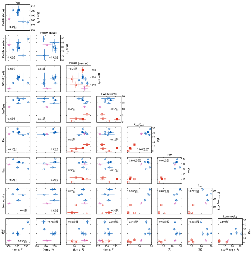
Figure 6: Corner plot of the Ly$\alpha$ measurements, as well as $f_{\text{esc}}^{\text{LyC}}$. Red squares are non-LyC-leaking apertures, blue circles are LyC-leaking apertures, and the pink star is slit M3. Filled markers are the stacked spectra. The value annotated in each plot indicates the Pearson correlation coefficient between the two quantities. Table 5 also lists the Pearson correlation coefficients and type ‘b’ Kendall rank correlation coefficients.

Surprisingly, the Ly$\alpha$ peak separation $v_{\rm{sep}}$ and $f_{\rm{esc}}^{\rm{LyC}}$ show a very significant positive correlation ($r=0.93_{-0.05}^{+0.03}$), contrary to the literature consensus of a negative correlation between the (galaxy-integrated) $v_{\rm{sep}}$ and $f_{\rm{esc}}^{\rm{LyC}}$. This unexpected result may be due to several factors. First, the peculiar shapes of some of the blueshifted Ly$\alpha$ peaks (namely slits M0, M2, and M9 in Figure 2, which appear slightly asymmetric relative to the fitted Ly$\alpha$ peak’s center) near their center may obfuscate the determination of an accurate Ly$\alpha$ peak separation since we have assumed their skewed Gaussianity (see § 4.2 for more discussion). Furthermore, the dynamic range of $v_{\rm{sep}}$ measured from the spectra is minimal and slit M3 impacts the correlation as a clear outlier to the other data points (Figure 6). The resolutions of the spectra ($R\gtrsim 5000$) are sufficiently high that they may be beginning to resolve departures from the skewed Gaussianity assumption, and thus also the simple shell model geometry and kinematics typically invoked to explain double-peaked LAEs. And because the spectra target small source plane areas, they should be more sensitive to any local departures from an idealized shell model. Also, the established $v_{\rm{sep}}-f_{\rm{esc}}^{\rm{LyC}}$ anticorrelation paradigm has mostly been built from double-peaked LAEs that suggest a much different mode for LyC escape—where LyC photons may escape because the optical depth of H I is sufficiently low that many LyC photons do not interact with the H I. This is not the dominant mode of LyC escape in the Sunburst Arc, where LyC photons primarily escape through an extremely underdense, thin channel (Rivera-Thorsen et al., 2017; Kim et al., 2023).

We found some moderate correlations and a strong anti-correlation among the measurement pairs including the FWHM of a Ly$\alpha$ peak, but no strong correlations (Table 5). We measured very similar FWHMs for all the redshifted and central Ly$\alpha$ peaks (excluding slits M4 and M5 in the latter, which had central Ly$\alpha$ peak FWHMs not much larger than the instrumental dispersion FWHM of $\sim 55$ km s^-1) (Table 4). The width of a Ly$\alpha$ peak should be sensitive to the number of scattering events the signal experiences before escaping the galaxy, but we found no clear correlations between the Ly$\alpha$ peak FWHM and other proxies for the H I scattering environment. However, the FWHM measurements suffer from fewer data points (indicating where a certain Ly$\alpha$ peak is not present in a profile). Additionally, there is little dynamic range in any of the FWHMs, which fundamentally limits the data’s sensitivity to any correlations between FWHMs and other quantities.

The strength of all the measured correlations are subject to caveats. In total, the spectra only target $\lesssim 10$ distinct regions in the galaxy’s source plane (Figure 7). Of those regions, the LyC-leaking apertures capture one region, and the non-LyC-leaking apertures capture the remaining regions. But based upon the source plane reconstruction (Figure 7), the non-LyC-leaking apertures (perhaps excluding slit M6 based upon its geometry) could each include significant contributions from multiple regions of the galaxy. This complicates the interpretation of their Ly$\alpha$ properties since the light in the apertures are the sum of multiple galaxy environments. Also, the LyC-leaking apertures dominate the sample size of many of the parameters and tend to cluster together since they target the same source plane object. This means slit M3, often an outlier to the LyC-leaking region’s sample despite also showing a triple-peaked Ly$\alpha$ profile (Figure 6), can greatly impact the apparent relation between two measurements.

Additionally, with enough measurements compared against each other, spurious correlations are virtually certain (dubbed data dredging, data snooping, or $p$-hacking). We made 36 comparisons between 9 measurements, with few data points ($5-11$ for any given comparison), so we cannot entirely discount a false detection of a correlation at the measured uncertainties.

4.1 $f_{\text{esc}}^{\text{LyC}}$

We found higher $f_{\text{esc}}^{\text{LyC}}$ in the MagE apertures targeting images Rivera-Thorsen et al. (2019) identified as LyC leakers ($\gtrsim 20\%$) than those targeting non-LyC-leaking images ($\lesssim 5\%$) (Table 3). Despite the larger aperture size and PSF of the MagE observations compared to the data and methodology of Rivera-Thorsen et al. (2019), the $f_{\text{esc}}^{\text{LyC}}$ of the LyC-leaking apertures are comparable to or only slightly lower than what Rivera-Thorsen et al. (2019) reported. For comparison, Rivera-Thorsen et al. (2019) reported a median absolute, IGM absorption-corrected LyC escape fraction from their apertures on the LyC-leaking region of $\approx 32\%$. Table 3 summarizes the measured HST photometry and $f_{\rm esc}^{\rm LyC}$.

As expected, the non-LyC-leaking apertures show no obvious LyC emission in the F275W image (Figure 4) and minimal $f_{\text{esc}}^{\text{LyC}}$ in our measurements, which use deeper rest-LyC imaging than Rivera-Thorsen et al. (2019) (5413 s versus 86902 s). The F275W image of the LyC-leaking images reveals that the LyC emission is extremely compact (Figure 4), and at the resolution of HST, the non-LyC-leaking slit apertures do not cover any images of the LyC leaker. Due to the convolution of the data with the ground-based seeing conditions (§ 3.4), some non-LyC-leaking images may have smaller $f_{\text{esc}}^{\text{LyC}}$ than suggested by this work’s aperture-based measurements because the simulation can cause LyC flux from nearby LyC-leaking images to enter the aperture. Since so little LyC flux should already be in a non-LyC-leaking aperture before the convolution, even a small amount could cause a large proportional change, but this likely only affects slit M3, and to a lesser extent slit M4, due to their proximity to images of the LyC-leaking region (Figure 1).

The LyC-leaking apertures show similar or slightly lower $f_{\text{esc}}^{\text{LyC}}$ than the corresponding median absolute, IGM absorption-corrected LyC escape fraction measurement in Rivera-Thorsen et al. (2019). We suggest two factors that may cause this reduction. First, the $f_{\text{esc}}^{\text{LyC}}$ calculation is inversely proportional to the F814W flux. Since our aperture (in effect of order $\sim 0.85\arcsec$ (slit width) $\times$ $1.7\arcsec$ (radial arc width)) is much larger than what Rivera-Thorsen et al. (2019) used ($\sim 0.12\arcsec\times 0.12\arcsec$), it is more sensitive to the F814W emission, which is more extended than the compact LyC emission in F275W. This means the F814W flux can effectively dilute the $f_{\text{esc}}^{\text{LyC}}$. Second, the convolution of the data with the ground-based seeing conditions (§ 3.4) introduces an artificial aperture loss: some LyC flux leaves an aperture due to the PSF of the ground-based seeing conditions, decreasing $f_{\text{esc}}^{\text{LyC}}$. This affects the LyC-leaking apertures more significantly due to the comparably-sized slit width and PSF. A possible exception is slit M2 (and slit M8 less so), where the slit placement’s immediate proximity to the LyC-leaking image 1.9 (Figure 1) suggests nontrivial LyC flux from image 1.9 enters its aperture, even though slit M2 does not directly cover it. This is reflected in slit M2’s $f_{\text{esc}}^{\text{LyC}}$, second in strength only to slit M0. A similar process may happen in slit M0 as LyC flux from image 1.6 of the LyC-leaking region enters the aperture. Slit M0 may have an exceptionally high LyC escape fraction because it covers 2 images of the LyC-leaking region—slit M0’s LyC escape fraction is also roughly double the LyC escape fractions of the other LyC-leaking apertures.

Table 5: Correlations between Ly$\alpha$ and LyC parameters

	$r$	$\tau$
FWHM (b) - $v_{\rm{sep}}$	$-0.4_{-0.2}^{+0.2}$	$-0.2_{-0.2}^{+0.2}$
FWHM (c) - $v_{\rm{sep}}$	$0.1_{-0.3}^{+0.4}$	$0.0_{-0.2}^{+0.3}$
FWHM (r) - $v_{\rm{sep}}$	$0.4_{-0.2}^{+0.2}$	$0.3_{-0.2}^{+0.2}$
$f_{\rm{min}}/f_{\rm{cont}}$ - $v_{\rm{sep}}$	$0.4_{-0.2}^{+0.1}$	$0.1_{-0.1}^{+0.2}$
Ly$\alpha$ EW - $v_{\rm{sep}}$	$-0.2_{-0.2}^{+0.2}$	$-0.1_{-0.2}^{+0.2}$
$f_{\rm{cen}}$ - $v_{\rm{sep}}$	$-0.5_{-0.1}^{+0.1}$	$-0.3_{-0.1}^{+0.1}$
Ly$\alpha$ $L$ - $v_{\rm{sep}}$	$0.4_{-0.2}^{+0.2}$	$0.2_{-0}^{+0.2}$
$f_{\rm{esc}}^{\rm{LyC}}$ - $v_{\rm{sep}}$	$0.93_{-0.05}^{+0.03}$	$0.7_{-0.1}^{+0.1}$
FWHM (c) - FWHM (b)	$-0.3_{-0.3}^{+0.3}$	$-0.2_{-0.2}^{+0.3}$
FWHM (r) - FWHM (b)	$0.5_{-0.4}^{+0.2}$	$0.3_{-0.3}^{+0.2}$
$f_{\rm{min}}/f_{\rm{cont}}$ - FWHM (b)	$0.1_{-0.3}^{+0.3}$	$0.0_{-0.2}^{+0.2}$
Ly$\alpha$ EW - FWHM (b)	$0.5_{-0.2}^{+0.2}$	$0.4_{-0.2}^{+0.2}$
$f_{\rm{cen}}$ - FWHM (b)	$0.5_{-0.2}^{+0.2}$	$0.4_{-0.2}^{+0.2}$
Ly$\alpha$ $L$ - FWHM (b)	$0.2_{-0.3}^{+0.3}$	$0.2_{-0.2}^{+0.4}$
$f_{\rm{esc}}^{\rm{LyC}}$ - FWHM (b)	$-0.71_{-0.06}^{+0.08}$	$-0.5_{-0.1}^{+0.1}$
FWHM (r) - FWHM (c)	$-0.2_{-0.2}^{+0.2}$	$-0.2_{-0.2}^{+0.2}$
$f_{\rm{min}}/f_{\rm{cont}}$ - FWHM (c)	$0.4_{-0.2}^{+0.2}$	$0.1_{-0.2}^{+0.1}$
Ly$\alpha$ EW - FWHM (c)	$0.5_{-0.2}^{+0.2}$	$0.2_{-0.2}^{+0.2}$
$f_{\rm{cen}}$ - FWHM (c)	$0.3_{-0.2}^{+0.2}$	$0.1_{-0.2}^{+0.1}$
Ly$\alpha$ $L$ - FWHM (c)	$0.2_{-0.2}^{+0.2}$	$0.1_{-0.2}^{+0.1}$
$f_{\rm{esc}}^{\rm{LyC}}$ - FWHM (c)	$0.51_{-0.08}^{+0.08}$	$0.28_{-0.1}^{+0.06}$
$f_{\rm{min}}/f_{\rm{cont}}$ - FWHM (r)	$-0.1_{-0.2}^{+0.2}$	$0.1_{-0.1}^{+0.1}$
Ly$\alpha$ EW - FWHM (r)	$-0.1_{-0.2}^{+0.2}$	$0.1_{-0.1}^{+0.1}$
$f_{\rm{cen}}$ - FWHM (r)	$-0.1_{-0.2}^{+0.2}$	$0.0_{-0.1}^{+0.1}$
Ly$\alpha$ $L$ - FWHM (r)	$0.3_{-0.3}^{+0.2}$	$0.3_{-0.2}^{+0.1}$
$f_{\rm{esc}}^{\rm{LyC}}$ - FWHM (r)	$0.18_{-0.09}^{+0.09}$	$0.28_{-0.1}^{+0.06}$
Ly$\alpha$ EW - $f_{\rm{min}}/f_{\rm{cont}}$	$0.965_{-0.01}^{+0.009}$	$0.71_{-0.07}^{+0.07}$
$f_{\rm{cen}}$ - $f_{\rm{min}}/f_{\rm{cont}}$	$0.898_{-0.009}^{+0.009}$	$0.56_{-0.04}^{+0.04}$
Ly$\alpha$ $L$ - $f_{\rm{min}}/f_{\rm{cont}}$	$0.90_{-0.01}^{+0.01}$	$0.79_{-0.07}^{+0.07}$
$f_{\rm{esc}}^{\rm{LyC}}$ - $f_{\rm{min}}/f_{\rm{cont}}$	$0.74_{-0.07}^{+0.06}$	$0.61_{-0.06}^{+0.1}$
$f_{\rm{cen}}$ - Ly$\alpha$ EW	$0.91_{-0.01}^{+0.01}$	$0.60_{-0.07}^{+0.04}$
Ly$\alpha$ $L$ - Ly$\alpha$ EW	$0.85_{-0.02}^{+0.02}$	$0.71_{-0.07}^{+0.07}$
$f_{\rm{esc}}^{\rm{LyC}}$ - Ly$\alpha$ EW	$0.60_{-0.08}^{+0.07}$	$0.3_{-0.1}^{+0.1}$
Ly$\alpha$ $L$ - $f_{\rm{cen}}$	$0.79_{-0.01}^{+0.01}$	$0.6_{-0}^{+0}$
$f_{\rm{esc}}^{\rm{LyC}}$ - $f_{\rm{cen}}$	$0.50_{-0.08}^{+0.07}$	$0.33_{-0.1}^{+0.06}$
$f_{\rm{esc}}^{\rm{LyC}}$ - Ly$\alpha$ $L$	$0.50_{-0.07}^{+0.07}$	$0.33_{-0.1}^{+0.06}$

Note. — Statistical correlations between the Ly$\alpha$ parameters and $f_{\rm{esc}}^{\rm{LyC}}$. From left to right: the parameter pair, Pearson correlation coefficient $r$, and type ‘b’ Kendall rank correlation coefficient $\tau$. The minimal number of data points (no more than 11 for any pair of parameters) means there are not many unique values of $\tau$, which causes many of the listed values and uncertainties to be similar, or in extreme cases for high SNR parameter measurements, for the 16th and 84th percentiles listed to be the same value as the median.

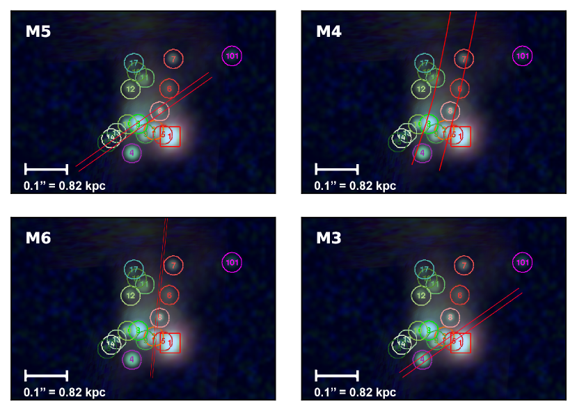
Figure 7: A portion of the approximate source plane reconstruction of the Sunburst Arc from Sharon et al. (2022) with ray-traced non-LyC-leaking apertures overlaid in red and labeled in the top left of each panel. The numbered circles and square correspond to the unique source plane regions identified in Sharon et al. (2022). Region 1 boxed in red is the LyC leaker.

4.2 Ly$\alpha$ properties

Our Ly$\alpha$ fitting (§ 3.5.4) well replicates the overall structure of each velocity profile (Figure 2, 3), but there are some residuals. Deviations from Gaussian or skewed Gaussian behavior are noticeable at the high spectral resolution and high signal-to-noise ratio (SNR) of the spectra, and likely reflect the fact that the outflowing H I gas has a much more complex geometry than the assumed isotropic shell used to justify the ad-hoc Gaussian and skewed Gaussian model. Key differences include the following:

• There is some excess flux in the red tails of the profiles not captured by the fits (Figures 2, 3). These features might reflect velocity intervals in the outflowing gas that have slightly higher column densities.

• The skewed Gaussian model fits to the Ly$\alpha$ peaks are not able to fully reproduce the shapes of the spectra. The strongest residual appears in slit M8’s redshifted Ly$\alpha$ peak fit (Figure 2), in which the data exhibit a sharper decline than the fit can produce. The impact of this effect on the line profile measurements is primarily an additional, small systematic error in the fitted FWHMs, biasing them slightly high.

• The centers of the redshifted Ly$\alpha$ peaks are often broader than the fits. This is especially clear in slits M6, M7, M8, and M9 (Figure 2). The minor emission peaks reported by Solhaug et al. (2024) at $\approx 130$ km s^-1 in high-resolution MIKE spectra (Figure 6 therein) may cause this, as the comparatively much lower resolution MagE spectra do not fully resolve these features.

• An absorber centered at $\sim 400$ km s^-1 attenuates the high-velocity tails of the blueshifted Ly$\alpha$ peaks, as also reported in Solhaug et al. (2024) with much higher resolution spectra. Additionally, the peak structure in several blueshifted Ly$\alpha$ peaks near their center seems more complex than a modest number of Gaussian or skew-Gaussian components can reproduce (particularly slits M0, M2, and M9 in Figure 2).

We also note that the structure of the redshifted Ly$\alpha$ peak is remarkably consistent across all of the spectra, indicating that it is likely a “global” feature. The remainder of this section discusses the measurements of the individual Ly$\alpha$ parameters. Table 4 summarizes the results.

4.2.1 Equivalent width

The Ly$\alpha$ EWs of the LyC-leaking apertures ($\sim 22-30$ Å) are higher than those of the non-LyC-leaking apertures ($\sim 4-12$ Å) by a factor of $\gtrsim 2$ (excepting slit M3; $24_{-1}^{+1}$ Å) (Table 4). Since Ly$\alpha$ photons primarily originate from H II regions, this strong difference is consistent with the much younger age of the LyC-leaking population ($3.3\pm 0.5$ Myr according to Mainali et al. (2022)).

4.2.2 Luminosity

We found $\text{log}_{10}(L_{\text{Ly}\alpha}(\text{ergs}^{-1}))\sim 41.4-42.2$ in non-LyC-leaking apertures and $\sim 42.2-42.5$ in LyC-leaking apertures (Table 4). The relationship between Ly$\alpha$ and LyC flux is not always clear. In principle, they are at odds, since LyC photons absorbed by H I increase the supply of H II ions that can recombine and emit Ly$\alpha$ photons. But a large $N_{\text{HI}}$ or dust content can effectively suppress both. The extinctions derived by Mainali et al. (2022) suggest the galaxy’s dust content does not vary significantly, indicating that older stellar populations in the non-LyC-leaking regions are the dominant effect causing the fainter Ly$\alpha$ luminosities.

4.2.3 $f_{cen}$

We found much higher $f_{\rm{cen}}$ in the LyC-leaking apertures ($\sim 20-30$%) than non-LyC-leaking ones ($\sim 7-10$%), except for slit M3 ($24.5_{-0.2}^{+0.2}$%) (Table 4). Naidu et al. (2022) previously measured $f_{\rm{cen}}\approx 37$% for the LyC leaker in the Sunburst Arc with archival X-SHOOTER data, though the area used to extract the spectrum in that work is unclear. Solhaug et al. (2024) also measured comparatively elevated $f_{\rm{cen}}$ with high-resolution MIKE spectra, finding $f_{\rm{cen}}\approx 42$% for the LyC-leaking region and $f_{\rm{cen}}\approx 37$% for approximately the same pointing as slit M3, which we judged to likely be a consequence of the much higher spectral resolution of their data ($R\approx 29,000$).

4.2.4 Peak widths and separation

Interestingly, the central and redshifted Ly$\alpha$ peak FWHMs are remarkably similar across most spectra (Table 4). The central Ly$\alpha$ peak FWHMs ($\sim 70-90$ km s^-1) are also consistent with the results of Solhaug et al. (2024), who measured central Ly$\alpha$ peak FWHMs of $\sim 71-95$ km s^-1 with the high-resolution ($R\approx 29,000$) Magellan/MIKE spectrograph for apertures approximately corresponding to slits M2, M3, and M0. The redshifted Ly$\alpha$ peak FWHMs are $\sim 230-250$ km s^-1, without significant difference between the LyC-leaking and non-LyC-leaking apertures. Some non-LyC-leaking spectra (specifically slits M3, M4, and M6) might have slightly narrower redshifted Ly$\alpha$ peaks than the LyC-leaking spectra, but the uncertainties make this unclear. If the difference is real, it conflicts with the expectation that the thicker H I column densities suspected to exist in the non-LyC-leaking regions should broaden emerging Ly$\alpha$ peaks and attenuate LyC flux. However, because the spectra (1) probe small distances in the source plane (much smaller than the galaxy-wide scales of most Ly$\alpha$ observations) and (2) show highly unique Ly$\alpha$ profiles indicative of much different H I geometry and kinematics than often observed, the same intuitions may not hold in this exotic object. The notable exception is the stacked spectrum of the non-LyC-leaking apertures, which has the broadest redshifted Ly$\alpha$ peak FWHM ($280_{-9}^{+9}$ km s^-1). This may be connected to possible degeneracies in the model fitting, since the central Ly$\alpha$ peak in the stacked spectrum of the non-LyC-leaking apertures is much fainter than the redshifted Ly$\alpha$ peak.

The blueshifted Ly$\alpha$ peak FWHMs are not so unusually behaved, but we may detect true differences between them (e.g., slit M0 versus slit M7) due to the larger scatter (Table 4). If genuine, it is unclear if these differences could be attributable to differential magnification of the images, the viewing angle into the LyC-leaking region, or other effects.

We measured Ly$\alpha$ peak separations $\sim 300-350$ km s^-1 in the LyC-leaking apertures and the non-LyC-leaking aperture slit M3 with a triple-peaked Ly$\alpha$ profile (Table 4). Low-redshift calibrations compiled by Izotov et al. (2022) suggest $f_{\rm{esc}}^{\rm{LyC}}\lesssim 10\%$ based upon these peak separations, much lower than the $f_{\rm{esc}}^{\rm{LyC}}\gtrsim 20\%$ we measured for the LyC-leaking apertures (Table 3). The exception is slit M3, which, despite its narrow peak separation ($302_{-7}^{+6}$ km s^-1), has a small LyC escape fraction ($f_{\rm{esc}}^{\rm{LyC}}=5\pm 3\%$). As noted in § 4.1, this may be an overestimate due to the simulated seeing effects (§ 3.4), as an image of the LyC-leaking region is near ($<1\arcsec$) the slit M3 aperture (Figure 1).

4.2.5 $f_{\rm{min}}/f_{\rm{cont}}$

We measured $f_{\rm{min}}/f_{\rm{cont}}\sim 14-19$ in the LyC-leaking spectra, similar to Green Pea galaxies (GPs) with the narrowest Ly$\alpha$ peak separations (Jaskot et al., 2019). In the non-LyC-leaking spectra, excluding slit M3 ($f_{\rm min}/f_{\rm cont}=11.5_{-0.5}^{+0.4}$), we found $f_{\rm{min}}/f_{\rm{cont}}\sim 1-6$, comparable to many GPs with wider peak separations (Jaskot et al., 2019). However, the driving cause of the $f_{\rm{min}}/f_{\rm{cont}}$ measured here is a directly escaping, separate Ly$\alpha$ peak. In most other works the measured $f_{\rm{min}}$ is consistent with two superimposed Ly$\alpha$ peaks expected from an isotropically expanding H I shell. This geometry is not representative of the Sunburst Arc since the central Ly$\alpha$ peak suggests a highly anisotropic ISM.

5 Discussion

A key piece in connecting Ly$\alpha$ and LyC escape in the Sunburst Arc is to explain the variety of Ly$\alpha$ profiles, especially the non-LyC-leaking apertures that show a triple-peaked Ly$\alpha$ profile or a central and redshifted Ly$\alpha$ peak. The essential picture explaining the triple-peaked Ly$\alpha$ profile observed in the images of the LyC leaker is well understood. Rivera-Thorsen et al. (2017) posited an ionized channel in a surrounding H I shell as the most likely mechanism to observe a triple peak structure. The much larger $f_{\text{cen}}$, $f_{\text{esc}}^{\text{LyC}}$, and Ly$\alpha$ escape fraction (Kim et al., 2023), and exceptionally blue UV slope (Kim et al., 2023) of the LyC-leaking region supports the existence of such a channel oriented along the sightline to the LyC-leaking region. The young age of the LyC leaker suggested by stellar population fitting, in tandem with its strong UV stellar feedback features (e.g., the N V 1238, 1242 Å, C IV 1548, 1550 $\text{\AA}$ doublets with P-Cygni wind profiles shown in Mainali et al. 2022) and compact size ($r_{\text{eff}}\lesssim 32$ pc (Sharon et al., 2022)), indicate an obvious culprit with the strong LyC flux and outflows suited to puncture the surrounding H I medium and leak LyC photons.

What remains unclear are the mechanisms leading to the observed non-LyC-leaking Ly$\alpha$ profiles, since multiple show a central Ly$\alpha$ peak (slits M4, M6, and M3), and in the case of slit M3, a triple-peaked Ly$\alpha$ profile (Figure 2). In the channel escape hypothesis, these are both associated with the presence of a LyC source, which do not appear in these apertures (Figure 4).

We have considered if differential magnification effects due to gravitational lensing could explain the observed non-LyC-leaking Ly$\alpha$ profiles. This scenario would require a high magnification gradient, which often occurs close to the critical curve (i.e., Figures 5, 6 in Sharon et al., 2022), and can increase or decrease the weighting of the different physical regions within a lensed galaxy in the spectra that we observe. However, a simple analysis using the lens model (Sharon et al., 2022) rejects this as a plausible explanation for the spatially variable Ly$\alpha$ and LyC properties of the Sunburst Arc. In the remainder of this section, we first highlight the peculiar nature of slit M3, which contains a peculiar source and a triple-peaked Ly$\alpha$ profile, but no significant escaping LyC flux. We then discuss possible explanations for all of the observed Ly$\alpha$ profiles in the MagE spectra.

5.1 A triple-peaked Ly$\alpha$ profile without LyC escape

Slit M3 stands out as the only non-LyC-leaking aperture with a triple-peaked Ly$\alpha$ profile, including a blueshifted Ly$\alpha$ peak with a slightly smaller blueshifted velocity than the blueshifted Ly$\alpha$ peak in the LyC-leaking apertures. The brightest continuum source in slit M3 (image 4.8 in Figure 1) has been dubbed Tr (Vanzella et al., 2020b), Godzilla (Diego et al., 2022; Choe et al., 2024; Pascale & Dai, 2024), and “the discrepant clump” (Sharon et al., 2022). The literature favors this object as stellar in nature, and we will refer to it as image 4.8, following Sharon et al. (2022). Here we discuss the Ly$\alpha$ and LyC escape properties of this object.

A natural starting assumption is to attribute the Ly$\alpha$ emission in slit M3 to the brightest continuum source captured by the slit, which is image 4.8. However, the Ly$\alpha$ narrowband maps from the WFC3/F410M image reveal that image 4.8 itself is mostly likely a net Ly$\alpha$ absorber, with the other diffuse arc flux that falls into slit M3 producing the observed Ly$\alpha$ emission. Inspecting slit M3’s position in the source plane reconstruction indicates that the emission captured by slit M3 comes from two physically distinct parts of the galaxy: region 4, and diffuse emission from or between regions 1, 2, and 5. This is notable because this diffuse emission in slit M3 comes from a region that is closer to the LyC-leaking region (but without containing the LyC-leaking region itself) than any other of the MagE slit apertures.

We observe LyC flux in slit M3’s aperture statistically consistent with zero flux (at $2\sigma$ confidence; Table 3). However, the young age ($\sim 4$ Myr), low stellar extinction of $\text{E}(\text{B}-\text{V})=0.018$ (the lowest measured in the MagE data; Mainali et al., 2022), and narrow Ly$\alpha$ peak separation suggest a low H I column density and a favorable stellar population and line of sight for LyC escape. However, it is difficult to tie all of these characteristics to the same physical region, since slit M3 covers emission regions separated by $\sim$1 kpc in the source plane (Figure 7). Here we review how the different physical natures offered for image 4.8 in the literature connect to the Ly$\alpha$ and LyC observations presented in this paper.

• A supernova. Vanzella et al. (2020b) first discussed the main image’s identity, positing it to be a transient stellar object, evidenced by the lack of counterimages, and the lack of any other object with the same unique spectroscopic signatures, namely Bowen fluorescence (Bowen, 1934). Based on their predicted magnification ($20<\mu<100$) and corresponding absolute magnitude ($-20.3<M_{2000}<-18.6$) of the main image, they favored a supernova and disfavored a luminous blue variable (LBV) star as too faint. However, detailed lens modeling by Diego et al. (2022) and Sharon et al. (2022) jointly corroborated that (1) the magnification of the main image must be extremely high ($\mu>600$), (2) the source plane persistence of the main image is exceptionally long for a supernova ($>1$ year), and (3) the predicted time delays for this source between different images ($<1$ year) are significantly shorter than the elapsed time of observations. The lack of appearance of any new, comparably bright images of “Godzilla” over $>7$ years strongly disfavors the supernova hypothesis. The lack of Ly$\alpha$ and LyC emission from image 4.8 is consistent with a SN.

• A luminous blue variable star. In contrast, Diego et al. (2022) suggested the largest knot in slit M3 could be a luminous blue variable (LBV) star in outburst. This could explain the observed Ly$\alpha$ signature and faint LyC detection, as well as rest-UV spectral features (Vanzella et al., 2020b). Quiescent LBVs are often B-type stars with temperatures ranging between $\sim 10000-25000$ K, but during their outbursts, they cool to $\sim 8500$ K and shed their outer layers as large mass outflows. Assuming the star’s quiescent temperature is among the hotter LBVs, the star may produce appreciable LyC flux. The radiative and mechanical energy from the LBV during an active phase could clear an underdense channel in the surrounding H I, but this picture is in tension with Choe et al. (2024), who concluded from JWST/NIRSpec IFU observations that the main image is a quiescent LBV, not an outbursting LBV. Furthermore, the dense gas required to pump Bowen fluorescence would naturally suppress escaping Ly$\alpha$ and LyC emission from the LBV, consistent with the observed lack of Ly$\alpha$ and LyC emission from image 4.8

As we explore physical hypotheses to explain the observed Ly$\alpha$ profiles below, it is important to remember that any plausible scenario must explain how slit M3 could show both central and blueshifted Ly$\alpha$ peaks but no escaping LyC photons.

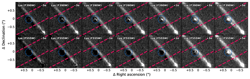
Figure 8: Ly$\alpha$ maps centered on slit M3 created from the schemes discussed in § 3.3. The top and bottom rows show the maps with the F390W and F555W filters as the off-band filter, respectively. The dashed magenta line is the on-sky aperture of slit M3. There are systematic differences between the two continuum subtraction bands, with the F555W-based subtraction removing marginally more continuum flux than the F390W-based subtraction

.

5.2 Seeing effects

We have considered if ground-based seeing conditions cause the unique kinematic structure of the Ly$\alpha$ profiles of the non-LyC-leaking apertures by diffusing images of the LyC leaker’s triple-peaked Ly$\alpha$ profile into non-LyC-leaking apertures. To judge this, we simulated the atmospheric diffusion with the Ly$\alpha$ maps discussed in § 3.3. For each slit aperture, we convolved each Ly$\alpha$ map with a 2-dimensional Gaussian kernel with width matching the time-weighted average of the combined effect of the seeing conditions (see Table 1 for a time-weighted average of the seeing conditions for each slit) and airmass for each exposure (Table 1). We then calculated the flux inside each slit aperture before and after the convolution and the ratio between those fluxes for each Ly$\alpha$ map. Table 6 contains the results.

In both the Ly$\alpha$ maps made from the F555W- and F390W-based continuum subtraction, we found that the LyC-leaking apertures lose Ly$\alpha$ flux ($\sim 10-40\%$) and the non-LyC-leaking slits mostly gain Ly$\alpha$ flux ($\sim 5-800\%$). The one exception is slit M5, which has a pre- and post-convolution flux that is statistically consistent to within $\sim 2\sigma$ in both continuum subtraction schemes.

We now outline how each non-LyC-leaking aperture fits into the seeing effects hypothesis, roughly in order of the apertures nearest to farthest from images of the LyC-leaking region on the sky.

• Slit M3 is roughly the non-LyC-leaking aperture nearest to images of the LyC-leaking region (Figure 4) and the only non-LyC-leaking aperture that has a blueshifted Ly$\alpha$ peak. This slit is the most consistent with the seeing effects hypothesis since it shows the hallmark triple-peaked Ly$\alpha$ profile of the LyC leaker and is $<1\arcsec$ away from the nearest image of the LyC-leaking region. Slit M3’s Ly$\alpha$ flux either changes significantly or minimally in the simulated seeing convolution, depending on the Ly$\alpha$ map (Table 6). This ambiguity is because the F555W-based Ly$\alpha$ map predicts strong Ly$\alpha$ absorption near and on the images in slit M3 (Figure 8). Additionally, slit M3’s blueshifted Ly$\alpha$ peak is distinctly closer to the systemic redshift than the blueshifted Ly$\alpha$ peaks observed from the LyC-leaking region (Figure 2, Table 7), which point to a different physical origin for slit M3’s blueshifted Ly$\alpha$ peak than simple seeing effects.

• Slit M4 is farther from the nearest images of the LyC-leaking region than slit M3, but still close enough ($\sim 1\arcsec$) that seeing effects could cause some contamination (Figure 4). Similar to slit M3, the Ly$\alpha$ flux in the aperture either changes significantly or minimally after the simulated seeing convolution, depending on the Ly$\alpha$ map (Table 6). Most importantly, slit M4 does not show a blueshifted Ly$\alpha$ peak (Figure 2), which we would expect to see if significant Ly$\alpha$ flux from the LyC-leaking region diffused into this slit due to seeing effects.

• Slit M6 is well-separated from the closest images of the LyC-leaking region (Figure 4), but still has a strong central Ly$\alpha$ peak, though no blueshifted Ly$\alpha$ peak. At most, the seeing-convolved Ly$\alpha$ images predict a moderately increased Ly$\alpha$ flux due to seeing effects. The absolute, magnification-uncorrected strength of slit M6’s central Ly$\alpha$ peak is several times greater than that of slit M4 (Table 7), even though slit M4 is closer to images of the LyC-leaking region. This fact (and the nonobservation of a blueshifted Ly$\alpha$ peak) strongly disfavors the seeing effects hypothesis since an aperture (slit M6) farther from images known to emit a central Ly$\alpha$ peak has a stronger central Ly$\alpha$ peak than another, closer aperture (slit M4).

• Slit M5 shows no distinct central or blueshifted Ly$\alpha$ peak and is one of the non-LyC-leaking apertures farthest from images of the LyC leaker (Figure 4), which is consistent with the seeing effects hypothesis. Like slit M6, the simulated seeing convolution predicts a minimal or moderate increase in Ly$\alpha$ flux in the slit M5 aperture due to the observing conditions (Table 6).

Table 6: Simulated aperture flux changes due to atmospheric seeing

Slit		F390W			F555W
	Unconvolved	Convolved	Ratio	Unconvolved	Convolved	Ratio
	[$e^{-}$ s-1]	[$e^{-}$ s-1]		[$e^{-}$ s-1]	[$e^{-}$ s-1]
M5	$0.82\pm 0.03$	$0.86\pm 0.03$	$1.05\pm 0.05$	$-0.15\pm 0.04$	$-0.21\pm 0.04$	$1.4\pm 0.5$
M4	$1.34\pm 0.03$	$1.42\pm 0.03$	$1.06\pm 0.03$	$0.04\pm 0.04$	$0.35\pm 0.04$	$10\pm 10$
M6	$1.66\pm 0.03$	$1.80\pm 0.03$	$1.08\pm 0.02$	$0.49\pm 0.04$	$0.81\pm 0.04$	$1.6\pm 0.2$
M3	$1.51\pm 0.04$	$1.61\pm 0.04$	$1.06\pm 0.04$	$-0.24\pm 0.08$	$0.25\pm 0.08$	$-1.0\pm 0.5$
M0	$5.90\pm 0.06$	$4.40\pm 0.06$	$0.75\pm 0.01$	$3.6\pm 0.1$	$2.8\pm 0.1$	$0.78\pm 0.04$
M2	$6.63\pm 0.07$	$5.10\pm 0.07$	$0.77\pm 0.01$	$5.2\pm 0.1$	$4.0\pm 0.1$	$0.77\pm 0.03$
M7	$3.22\pm 0.04$	$2.50\pm 0.04$	$0.78\pm 0.01$	$2.18\pm 0.07$	$1.70\pm 0.07$	$0.78\pm 0.04$
M8	$2.49\pm 0.02$	$2.21\pm 0.02$	$0.89\pm 0.01$	$1.98\pm 0.04$	$1.79\pm 0.04$	$0.90\pm 0.03$
M9	$3.02\pm 0.03$	$2.43\pm 0.03$	$0.80\pm 0.01$	$2.27\pm 0.06$	$1.46\pm 0.06$	$0.64\pm 0.03$

Note. — From left to right: slit, flux inside the slit of the unconvolved and simulated seeing-convolved F390W-based Ly$\alpha$ map, the ratio between the two fluxes, and likewise for the F555W-based Ly$\alpha$ map. Ratios $>$ 1 indicate the flux in the aperture increased after the convolution, and ratios $<$ 1 indicate the flux in the aperture decreased after the convolution. The convolution used a 2-dimensional Gaussian kernel of the combined effect of the time-weighted seeing conditions and airmasses (§ 5.2).

Combined, the evidence above suggests seeing effects alone cannot explain all the Ly$\alpha$ profiles of the non-LyC-leaking apertures, but might affect their Ly$\alpha$ profiles in some instances—such as slit M3 due to its proximity to images of the LyC-leaking region. Because both ground-based seeing effects (§ 5.2) and differential magnification from gravitational lensing do not explain the observed Ly$\alpha$ profiles of the non-LyC-leaking apertures, we must consider explanations that invoke complex mechanisms and morphologies, which we explore below.

5.3 Multiple direct escape Ly$\alpha$ channels

Here we consider if additional ionized channels might also explain the central Ly$\alpha$ peaks observed from the non-LyC-leaking apertures. Any channel escape scenario must explain the observation of a central Ly$\alpha$ peak but not a blueshifted Ly$\alpha$ peak in some of the non-LyC-leaking apertures (slits M4 and M6). If the additional ionized channels are similar to the channel observed in the LyC-leaking region (i.e., additional small channels puncturing an isotropically expanding H I shell), then the gas along the sightlines toward the additional channels must have properties that permit Ly$\alpha$ photons to directly escape, but not LyC photons.

Such a scenario is difficult to construct because the cross section for Ly$\alpha$ photons to interact with H I is $\sim 10^{4}$ times higher than the cross section for LyC photon interactions. This means that if there is sufficiently low H I column density along a sightline to allow Ly$\alpha$ photons to escape with few or no scattering events (“direct escape” Ly$\alpha$), then LyC photons should also freely escape. Furthermore, a blueshifted Ly$\alpha$ peak is associated with outflowing gas with low H I column density. The lack of a blueshifted Ly$\alpha$ peak in some of the non-LyC-leaking apertures with a central Ly$\alpha$ peak requires either (1) simultaneously both high column density, outflowing H I and an extremely low column density H I channel puncturing it, or (2) a complete absence of outflowing H I. The former would require a sharp transition between the two gas phases to minimize the H I thin enough to transmit a blueshifted Ly$\alpha$ peak but thick enough to prevent direct Ly$\alpha$ scape, while the latter would allow LyC photons to efficiently escape (which we do not observe).

We also note that the stellar populations in the non-LyC-leaking regions of the Sunburst Arc have ages of $11.8\pm 0.9$ Myr (Mainali et al., 2022), which is notably older and should produce fewer LyC photons (Ma et al., 2015, 2020; Kimm et al., 2017; Kim et al., 2019; Kakiichi & Gronke, 2021) than the LyC leaking region’s age of $3.3\pm 0.5$ Myr (Mainali et al., 2022). The rest-UV absorption lines and nebular emission lines in the non-LyC-leaking spectra also indicate weaker stellar winds, bulk outflows (Mainali et al., 2022), and less extreme ionizing radiation fields (Kim et al., 2023) than the LyC-leaking region, meaning the non-LyC-leaking regions are less well-suited to create ionized channels. This makes it physically unlikely for the non-LyC-leaking regions to be able to create additional highly ionized channels, especially considering that radiative transfer simulations predict channels to be extremely rare (e.g., Behrens et al., 2014).

5.4 A Ly$\alpha$ mirror

We now introduce a Ly$\alpha$ ‘mirror’ hypothesis, which posits that dense H I cores could preferentially scatter Ly$\alpha$ photons from the LyC-leaking region into our sightline far from their origin. As discussed in § 1, Ly$\alpha$ photons may wander far from their birthplace before scattering into our sightline. The central Ly$\alpha$ peak observed in some of the non-LyC-leaking apertures might be an extreme case of this: Ly$\alpha$ photons of the LyC-leaking region incident upon dense H I gas surrounding the non-LyC-leaking regions may preferentially scatter off of the cores’ surfaces and cause apparent Ly$\alpha$ emission from regions physically distant from the original Ly$\alpha$ source.

This preferential scattering is similar to the mechanism that produces the redshifted Ly$\alpha$ peak in an isotropically expanding H I shell geometry (e.g., Figure 12 in Verhamme et al., 2006). If this process involved only a few scatterings then the central Ly$\alpha$ peak may survive, albeit diminished, which is what we observe in the non-LyC-leaking apertures that are closest to the LyC-leaking region in the source plane (Figure 2). This would require either a large region with very low column density H I and/or very fast (i.e., out of resonance) outflowing gas between the “mirror” and our sightline to allow the central Ly$\alpha$ photons to escape. The strong ionizing photon flux of the LyC-leaking region may aid this process by creating a large ionized region inside the galaxy, allowing Ly$\alpha$ photons to traverse large distances far from their birth place. Figure 9 sketches out this hypothesis.

We now outline how this hypothesis connects to the Ly$\alpha$ profiles of each non-LyC-leaking aperture, in order of the strongest to weakest central Ly$\alpha$ peaks, relative to their associated redshifted Ly$\alpha$ peaks.

• This aperture covers parts of regions 1, 2, 4, 5, and 9 in the source plane (Figure 7). Slit M3 is the closest non-LyC-leaking aperture to the LyC-leaking region, meaning some of the area it covers—namely regions 1, 2, and 5—could receive the necessary Ly$\alpha$ flux to scatter into our sightline before significant Ly$\alpha$ photons scatter prematurely, attenuate, or become too diffuse. If a Ly$\alpha$ ‘mirror’ causes slit M3’s strong central Ly$\alpha$ peak, there must be very few scatterings and a strong directional bias toward us to preserve a central Ly$\alpha$ peak that is nearly as strong (relative to the spectrum’s other Ly$\alpha$ peaks) as in the LyC-leaking apertures. There must also be very low column density outflowing H I in this region to explain the presence of a blueshifted Ly$\alpha$ peak in slit M3. The lack of LyC photons within this aperture suggests that that there are no bright LyC photon sources in the diffuse emission captured by slit M3, such that the Ly$\alpha$ emission detected from this slit is the product of Ly$\alpha$ photons that diffused away from the LyC-leaking region before scattering into our sightline.

• This aperture covers parts of regions 2, 5, and 8. Slit M6’s central Ly$\alpha$ peak is comparable in strength to its redshifted Ly$\alpha$ peak (Figure 2) and its projected distance to the LyC-leaking region in the source plane is farther than for slit M3 (Figure 7). The central Ly$\alpha$ peak of slit M6 could also result from the “mirror” effect. Slit M6’s larger distance from the LyC-leaking region might explain the weaker central Ly$\alpha$ peak (relative to the redshifted Ly$\alpha$ peak) compared to the LyC-leaking region due to some combination of (1) a smaller covering fraction of the mirror for slit M6 than slit M3, and (2) an increasing number of scattering events for Ly$\alpha$ photons as they travel farther from their original source in the LyC-leaking region.

• This aperture targets a lower magnification region of the arc and therefore covers a large portion of the lensed galaxy in the source plane, including regions $2-11$. Though parts of the slit are closer to the LyC-leaking region in the source plane than slit M6 (Figure 7), its central Ly$\alpha$ peak is much weaker compared to its redshifted Ly$\alpha$ peak than in slit M6, though the magnification-corrected central Ly$\alpha$ flux is still stronger absolutely than that of slit M6 (Figure 2, Table 7). This makes sense given the large footprint of slit M4 in the source plane if the redshifted Ly$\alpha$ peak is a global feature, while the central Ly$\alpha$ peak is not.

• This aperture covers parts of regions 3, $8-10$, and $13-15$. Of all the non-LyC-leak apertures, it has the largest projected distance from the LyC-leaking region in the source plane, and it is the only non-LyC-leaking aperture with no clear central Ly$\alpha$ peak. This implies a minimum upper limit on the extent of the central Ly$\alpha$ peak of $\lesssim 800$ pc.

If a Ly$\alpha$ mirror does exist, it extends to at least clumps 1, 2, 5, and 9 in Figure 7, since those clumps define a region of overlap between slits that show a central Ly$\alpha$ peak (M3, M4, and M6). This suggests a “direct escape” Ly$\alpha$ region extending as much as $\sim 600-800$ pc from the LyC-leaking region.

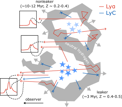
Figure 9: Cartoon of the Ly$\alpha$ mirror hypothesis. The LyC-leaking region (bottom) produces a prodigious amount of Ly$\alpha$ (red) and LyC (blue) photons compared to the older non-LyC-leaking regions (top). Some photons from the LyC-leaking region directly escape out of a highly ionized channel oriented toward us. These photons constitute the observed LyC and central Ly$\alpha$ peak. Additional Ly$\alpha$ emission resonantly scatters off the expanding H I surrounding the LyC-leaking region until it escapes the galaxy along the observer’s sightline, which constitute the redshifted and blueshifted Ly$\alpha$ peaks (bottom box). In the non-LyC-leaking regions, which have much less LyC flux due to their older age, the surrounding H I (gray) is thicker, preventing any LyC escape and direct Ly$\alpha$ escape. Thus, only a redshifted Ly$\alpha$ peak emerges (first box from the top). However, Ly$\alpha$ photons from the LyC-leaking region preferentially reflect into the observer’s sightline incident upon the thick H I around the non-LyC-leaking regions (second box from the top), forming a central Ly$\alpha$ peak superimposed upon the redshifted Ly$\alpha$ peak emerging from the non-LyC-leaking regions.

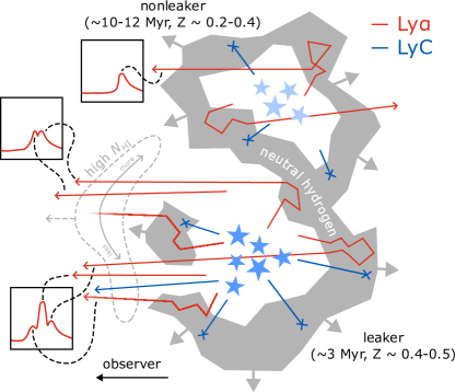
Figure 10: Cartoon sketch of the spatially variable absorption hypothesis. The Ly$\alpha$ and LyC photons directly escaping through an ionized channel produce the LyC and the central Ly$\alpha$ peak observed from the LyC-leaking region. Ly$\alpha$ photons from the LyC-leaking region also resonantly scatter with either side of the surrounding, expanding H I shell, forming the redshifted and blueshifted Ly$\alpha$ peaks (bottom box). In this picture, the triple-peaked Ly$\alpha$ profile from the LyC-leaking region originates from a large source plane area, and an intervening, outflowing absorber with higher HI column density attenuates the blueshifted Ly$\alpha$ peak and varying amounts of the central Ly$\alpha$ peak across the face of the galaxy.

5.5 Spatially variable Ly$\alpha$ absorption

The final hypothesis we present also relies on a complex H I morphology in the source plane. We suggest that the triple-peaked Ly$\alpha$ profile of the LyC-leaking region occupies an area in the source plane that is much larger than the clump producing the ionizing radiation (the LyC-leaking region). In this picture, the LyC-leaking region has ionized a huge volume of gas, producing the central Ly$\alpha$ peak over a large extent, as escaping Ly$\alpha$ photons can either form in-situ from the extended ionized gas, or travel large transverse distances in the source plane before experiencing scattering event(s) that redirect them into other, non-LyC-leaking sightlines.

The spatial variability of the blueshifted and central Ly$\alpha$ peaks’ strength is likely due to an outflowing (blueshifted) intervening absorber with H I column density that varies spatially across the face of the galaxy. For this absorber to screen the central Ly$\alpha$ peak, there must be additional highly ionized sightlines toward the extended ionized gas. For example, the H I surrounding the extended ionized gas may be patchy and heavily punctured. However, the H I cannot be significantly perforated, or there would not be sufficient approaching, outflowing H I to reprocess Ly$\alpha$ photons into the blueshifted Ly$\alpha$ peak that we see in slit M3 and the LyC-leaking apertures. Figure 10 depicts the basic principles of this scenario.

There are several key unknowns involved in this picture. First, what is the size and structure of the highly ionized, extended region around the LyC-leaking region? Second, what is the location and morphology of the neutral H I gas that absorbs LyC photons from all sightlines except those from a small channel toward the LyC-leaking region? The first question could be addressed in part by future spatially resolved measurements of the physical extent of forbidden (optically thin) nebular emission lines in the source plane. The second question, however, may require very specific H I morphology and kinematics to efficiently diffuse the directly escaping, central Ly$\alpha$ peak from the LyC-leaking region without completely rescattering it—perhaps not too dissimilar from the H I morphology and kinematics presumed in the mirror hypothesis of § 5.4—if most of the central Ly$\alpha$ peak’s photons do not form in-situ from the extended ionized gas.

Significant supporting evidence exists for this hypothesis. For instance, the neutral gas-tracing low ionization absorption analyzed by Mainali et al. (2022) suggests a blueshifted, low-ionization absorber exists along both LyC-leaking and non-LyC-leaking sightlines. That result is also consistent with the absorption trough at $\sim-350$ km s^-1 (Figure 2) that is present in all of the Ly$\alpha$ spectra. Furthermore, this blueshifted absorption trough has noticeably stronger absorption tails in the non-LyC-leaking MagE spectra, suggesting an absorption gradient between the LyC-leaking and non-LyC-leaking regions, with an increasing column density as the slits move farther away from the LyC-leaking region. This absorber might also explain the sharp drop-off on the blue side of the blueshifted Ly$\alpha$ peaks. Below, we explore how each non-LyC-leaking aperture might fit into this picture, in order of increasing projected distance from the LyC-leaking region, based on the source plane reconstruction (Figure 7) and Ly$\alpha$ profile fits (Figure 2).

• Of the non-LyC-leaking apertures, slit M3 is nearest to the LyC-leaking region in the source plane. It also shows the least signs of absorption compared to the LyC-leaking region’s Ly$\alpha$ profile, all of which is fully consistent with this physical picture. A very weak absorption process also provides the simplest and clearest explanation for slit M3’s blueshifted Ly$\alpha$ peak, which is slightly less blueshifted than the blueshifted Ly$\alpha$ peak in the LyC-leaking spectra. Similar to the Ly$\alpha$ mirror hypothesis above, the lack of LyC photons within this aperture suggests that all of the Ly$\alpha$ photons observed in slit M3 stem from Ly$\alpha$ photons that diffused or originated far from the LyC-leaking region before entering our sightline.

• Slit M4 is the next closest slit to the LyC-leaking region in the source plane, though it also has the largest footprint and captures many non-LyC-leaking regions distant from the LyC-leaking region. Slit M4 shows a suppressed central Ly$\alpha$ peak and no blueshifted Ly$\alpha$ peak. In the gradient absorber picture, this would indicate the absorber’s optical depth has grown, which is consistent with the increased distance of slit M4 to the LyC-leaking region in the source plane.

• Slit M6 has a very high magnification ($\mu=147_{-20}^{+5}$, Table 1), causing the slit to be very narrow in the source plane, isolating region 2. Slit M6 is an interesting contrast to slit M4 (which is one of the least magnified slits). Comparing the total, magnification-corrected flux in the central Ly$\alpha$ peaks of slits M6 and M4, there is significantly more flux in slit M4, but comparing the relative strengths of the central and redshifted Ly$\alpha$ peaks, it is clear slit M6’s central Ly$\alpha$ peak is stronger relative to the redshifted Ly$\alpha$ peak than in slit M4. This makes sense if (1) the redshifted Ly$\alpha$ peak is a global emission feature with approximately constant surface brightness across the entire source plane, and (2) the central Ly$\alpha$ peak emission is localized to a region that extends a few hundred parsecs around the LyC-leaking region. Slit M4 has a much larger footprint that could then contain Ly$\alpha$ profiles from other non-LyC-leaking regions (which slit M6 does not cover) with higher H I column densities and a more diminished or absent central Ly$\alpha$ peak and stronger absorption trough.

• Slit M5 is the farthest aperture from the LyC-leaking region in the source plane. It has no clear evidence of any residual blueshifted or central Ly$\alpha$ peak. Its Ly$\alpha$ profile could be consistent with a single redshifted Ly$\alpha$ peak. This slit is consistent with the redshifted Ly$\alpha$ peak as a global emission feature that extends across the entire galaxy. If the central Ly$\alpha$ peak’s production region extends as far as slit M5 in the source plane, then the intervening absorber along this slit’s sightline must have a very high H I column density to suppress the central Ly$\alpha$ emission. It is also possible that the physical extent of the region emitting the central Ly$\alpha$ peak ends somewhere between slits M6 and M5 in the source plane.

Combined, we believe that a diffuse triple-peaked Ly$\alpha$ profile combined with blueshifted H I absorption as a physical scenario has significant merit, especially considering the ubiquitous absorption trough in every Ly$\alpha$ profile.

Table 7: Ly$\alpha$ modeling best-fit parameters

Slit	Blue peak	Red peak	Central peak	Continuum
NL	$-$ / $-$ / $-$ / $-$	$3.74_{-0.07}^{+0.07}$ / $127_{-5}^{+5}$ / $210_{-4}^{+4}$ / $3.5_{-0.3}^{+0.4}$	$2.3_{-0.3}^{+0.3}$ / $60_{-5}^{+5}$ / $41_{-3}^{+2}$ / $-$	$1.17_{-0.02}^{+0.02}$
L	$6.58_{-0.07}^{+0.07}$ / $-99_{-2}^{+2}$ / $89_{-2}^{+2}$ / $-0.0002_{-0.003}^{+0.0002}$	$5.7_{-0.1}^{+0.1}$ / $157_{-6}^{+5}$ / $210_{-2}^{+3}$ / $5.3_{-0.8}^{+0.9}$	$22.6_{-0.4}^{+0.3}$ / $79_{-1}^{+1}$ / $41_{-1}^{+1}$ / $-$	$1.34_{-0.02}^{+0.02}$
M5	$-$ / $-$ / $-$ / $-$	$1.91_{-0.06}^{+0.06}$ / $121_{-4}^{+5}$ / $204_{-7}^{+7}$ / $5.1_{-0.7}^{+1}$	$0.6_{-0.2}^{+0.3}$ / $40_{-10}^{+20}$ / $30_{-10}^{+10}$ / $-$	$0.92_{-0.02}^{+0.02}$
M4	$-$ / $-$ / $-$ / $-$	$1.93_{-0.07}^{+0.07}$ / $128_{-4}^{+4}$ / $194_{-6}^{+6}$ / $6_{-1}^{+2}$	$1.7_{-0.1}^{+0.1}$ / $44_{-5}^{+6}$ / $36_{-4}^{+5}$ / $-$	$0.69_{-0.02}^{+0.02}$
M6	$-$ / $-$ / $-$ / $-$	$3.15_{-0.07}^{+0.1}$ / $175_{-5}^{+3}$ / $193_{-4}^{+4}$ / $6_{-2}^{+1}$	$5.1_{-0.2}^{+0.2}$ / $95_{-6}^{+3}$ / $45_{-3}^{+2}$ / $-$	$0.87_{-0.02}^{+0.02}$
M3	$3.56_{-0.09}^{+0.08}$ / $-66_{-6}^{+6}$ / $81_{-4}^{+4}$ / $-0.0004_{-0.004}^{+0.0004}$	$2.96_{-0.07}^{+0.07}$ / $168_{-4}^{+3}$ / $184_{-3}^{+4}$ / $5.0_{-0.8}^{+0.9}$	$7.5_{-0.3}^{+0.2}$ / $77_{-2}^{+2}$ / $42_{-2}^{+2}$ / $-$	$0.65_{-0.01}^{+0.01}$
M0	$55.4_{-0.9}^{+0.9}$ / $-105_{-2}^{+2}$ / $79_{-2}^{+2}$ / $-0.0009_{-0.002}^{+0.0008}$	$48.5_{-0.7}^{+0.8}$ / $186_{-3}^{+2}$ / $202_{-3}^{+3}$ / $6.5_{-0.7}^{+0.7}$	$208_{-2}^{+2}$ / $94.5_{-0.8}^{+0.7}$ / $46.6_{-1}^{+0.9}$ / $-$	$13.3_{-0.2}^{+0.2}$
M2	$3.6_{-1}^{+0.2}$ / $-102_{-7}^{+70}$ / $85_{-5}^{+40}$ / $-0.05_{-3}^{+0.05}$	$3.8_{-0.2}^{+0.2}$ / $160_{-10}^{+10}$ / $197_{-5}^{+6}$ / $4_{-1}^{+2}$	$18.1_{-0.8}^{+0.5}$ / $84_{-1}^{+2}$ / $38_{-1}^{+3}$ / $-$	$0.99_{-0.03}^{+0.03}$
M7	$5.22_{-0.07}^{+0.07}$ / $-103_{-3}^{+3}$ / $89_{-2}^{+2}$ / $-0.0008_{-0.003}^{+0.0008}$	$4.01_{-0.05}^{+0.06}$ / $150_{-3}^{+2}$ / $203_{-3}^{+2}$ / $7.4_{-0.9}^{+0.8}$	$16.1_{-0.2}^{+0.2}$ / $67.7_{-0.8}^{+0.7}$ / $40.6_{-1}^{+0.9}$ / $-$	$0.94_{-0.01}^{+0.01}$
M8	$4.77_{-0.07}^{+0.07}$ / $-91_{-3}^{+3}$ / $87_{-3}^{+3}$ / $-0.0006_{-0.003}^{+0.0006}$	$4.08_{-0.07}^{+0.1}$ / $168_{-7}^{+3}$ / $212_{-3}^{+4}$ / $7_{-2}^{+1}$	$16.6_{-0.3}^{+0.2}$ / $86_{-2}^{+1}$ / $42_{-2}^{+1}$ / $-$	$0.89_{-0.02}^{+0.02}$
M9	$2.89_{-0.08}^{+0.08}$ / $-100_{-4}^{+5}$ / $88_{-4}^{+5}$ / $-0.001_{-0.004}^{+0.001}$	$2.42_{-0.05}^{+0.06}$ / $170_{-3}^{+2}$ / $213_{-5}^{+5}$ / $8_{-2}^{+2}$	$9.6_{-0.2}^{+0.2}$ / $80_{-1}^{+1}$ / $43_{-1}^{+1}$ / $-$	$0.66_{-0.02}^{+0.02}$

Note. — Best-fit Ly$\alpha$ parameters of the magnification-uncorrected, rest-frame Ly$\alpha$ profiles. From left to right: slit label, best-fit parameters for the blueshifted peak, redshifted peak, and central peak, presented as $\alpha$/$\mu$/$\sigma$/$\omega$, as described in § 3.5.4. Apart from the stacked spectra, $\alpha$ has units of $10^{-16}$ erg s^-1 cm^-2 Å^-1, and $\mu$ and $\sigma$ have units of km s^-1.

6 Conclusions

In this work, we analyzed rest-UV, high-resolution ($R\sim 5000$) spectroscopy of the Ly$\alpha$ emission line in the Sunburst Arc (§ 2.1), a strongly lensed, LyC-leaking galaxy at $z\approx 2.37$. We directly fitted the Ly$\alpha$ velocity profiles to extract key parameters (§ 3.5) such as the peak separation $v_{\rm{sep}}$ (§ 3.5.4), peak widths (§ 3.5.4), Ly$\alpha$ equivalent width (§ 3.5.2), central escape fraction $f_{\rm{cen}}$ (§ 3.5.3), and ratio between the minimum flux density between the peaks and local continuum flux density $f_{\rm{min}}/f_{\rm{cont}}$ (§ 3.5.5). Using HST imaging (§ 2.2), we computed the LyC escape fractions associated with the spectroscopic observations (§ 3.4).

From this, we computed statistical correlations between the Ly$\alpha$ and LyC parameters to better understand their interdependence (§ 4), and offered brief discussion of the measurements of each parameter (§ 4.1, § 4.2.1–§ 4.2.5), and possible shortcomings of the Ly$\alpha$ profile fitting (§ 4.2). In short, we found:

• a strong positive correlation between $f_{\rm{esc}}^{\rm{LyC}}$ and $v_{\rm{sep}}$, $f_{\rm{min}}/f_{\rm{cont}}$, and Ly$\alpha$ EW (Table 5),

• few clear relations between any two parameters involving any of the Ly$\alpha$ peak widths (Table 5), and

• affirmations of previously suggested relations, especially a strong correlation between the Ly$\alpha$ EW and $f_{\rm{min}}/f_{\rm{cont}}$.

We also note that a central Ly$\alpha$ peak appears even in spectra of non-LyC-leaking regions from apertures located within $\sim 600$ pc of the LyC-leaking region. We briefly discussed the observed spectrum of the highly magnified region known as “Godzilla” and its implications for the nature of the object. Based upon the data and a source plane reconstruction of the slit aperture geometry (Figure 7), we discussed several possible explanations for the diversity of Ly$\alpha$ profiles observed in the Sunburst Arc (§ 5), particularly those from the non-LyC-leaking spectra. We first considered if ground-based seeing effects (§ 5.2) could cause the observed Ly$\alpha$ profiles by diffusing emission from images of the LyC-leaking region into the non-LyC-leaking slit apertures, but concluded that this mechanism cannot explain the data.

We then discussed physical mechanisms to explain the observed Ly$\alpha$ profiles of the non-LyC-leaking apertures (§ 5.3$-$§ 5.5). We concluded that the data are inconsistent with the presence of additional highly ionized channels that permit direct Ly$\alpha$ escape without LyC escape (§ 5.3). We then sketched out two physical scenarios—the Ly$\alpha$ mirror (§ 5.4) and the spatially variable Ly$\alpha$ absorber (§ 5.5)—to explain the presence of a central Ly$\alpha$ peak that originates from a much larger physical region than the escaping LyC photons.

The hypotheses we judged to be the strongest both invoke some form of spatially variable H I with complex morphology, geometry, and/or kinematics which can efficiently diffuse and/or preferentially rescatter a central Ly$\alpha$ peak, likely from the LyC-leaking region. In one scenario (§ 5.4), dense but perforated H I in the intermediate space between the LyC-leaking and non-LyC-leaking regions preferentially rescatters a central Ly$\alpha$ peak into our sightline with minimal velocity shift. In the second scenario (§ 5.5), the central Ly$\alpha$ peak actually occupies a much larger area in the source plane than the LyC-leaking region. Although the specific H I structure and role of absorption are unclear in this explanation, additionally invoking a blueshifted absorber likely offers the simplest explanation and is also consistent with the ubiquitous blueshifted Ly$\alpha$ absorption feature centered around $-350$ km s^-1. Low-ionization metal absorption lines seen toward the non-LyC-leaking regions also support the existence of such an absorber (Mainali et al., 2022).

Another important implication of the work presented here is the direct measurement of the complex, anisotropic relationship between the escape of Ly$\alpha$ and LyC photons, particularly on the small physical scales (hundreds of parsecs and less) probed in the strongly lensed Sunburst Arc. The individual ISM structures that shape Ly$\alpha$ and LyC escape vary at or below this physical scale, which may challenge intuition built from galaxy-integrated properties. The Sunburst Arc is an instructive example of this variability and the small, complex ISM structures we must consider as we develop our understanding of the Ly$\alpha$-LyC connection at sub-galactic scales. The central Ly$\alpha$ peaks without corresponding LyC escape presented in this work are a clear example of this conflict.

As wide-area surveys such as DECaLS, Pan-STARRS, SDSS, and soon Rubin’s Legacy Survey of Space and Time or the Roman Space Telescope’s High Latitude Wide Area Survey discover increasing numbers of strongly lensed galaxies, JWST and ELTs will target them with extremely sharp imaging and IFU spectroscopy. We will be able to routinely map distant galaxies down to scales of tens of parsecs or less. Until the discovery of more exceptional objects, the Sunburst Arc offers the highest spatial resolution view of the Ly$\alpha$ and LyC escape processes, and the best opportunity to reconcile disagreements between low and high spatial resolution Ly$\alpha$ and LyC observations.

7 Author Contributions

M.R.O. measured the Ly$\alpha$ parameters and $f_{\text{esc}}^{\text{LyC}}$ with advice from K.J.K., M.B.B., and T.E.R.-T. M.R.O. prepared the manuscript with comments and input from all coauthors. M.B.B. obtained the MagE spectra, which were reduced by J.R.R. M.D.G. reduced the HST data. K.S. developed the lens model, created the source plane reconstruction with ray-traced non-LyC-leaking apertures, and calculated the magnification of the MagE apertures. A.N. removed foreground contaminants from the HST imaging to properly estimate $f_{\text{esc}}^{\text{LyC}}$ and added details of this process to the manuscript. This relied upon PSF models created by M.F. with software written by M.D.G. J.G.B. contributed to the background modeling of the HST imaging. M.R.O. created the HST-based Ly$\alpha$ maps based upon software originally written by J.R.R. and SEDs made by G.K. with photometry measured by M.F. G.K. contributed details of the SED modeling to the manuscript.

8 Access

The software used to create the results of this paper—and the results themselves—are available freely and publicly on GitHub, including detailed documentation (Owens & Rigby, 2024).

References

- Astropy Collaboration et al. (2013) Astropy Collaboration, Robitaille, T. P., Tollerud, E. J., et al. 2013, A&A, 558, A33, doi: 10.1051/0004-6361/201322068
- Astropy Collaboration et al. (2018) Astropy Collaboration, Price-Whelan, A. M., Sipőcz, B. M., et al. 2018, AJ, 156, 123, doi: 10.3847/1538-3881/aabc4f
- Astropy Collaboration et al. (2022) Astropy Collaboration, Price-Whelan, A. M., Lim, P. L., et al. 2022, ApJ, 935, 167, doi: 10.3847/1538-4357/ac7c74
- Atek et al. (2023) Atek, H., Labbé, I., Furtak, L. J., et al. 2023, arXiv e-prints, arXiv:2308.08540, doi: 10.48550/arXiv.2308.08540
- Behrens et al. (2014) Behrens, C., Dijkstra, M., & Niemeyer, J. C. 2014, A&A, 563, A77, doi: 10.1051/0004-6361/201322949
- Bergvall et al. (2006) Bergvall, N., Zackrisson, E., Andersson, B. G., et al. 2006, A&A, 448, 513, doi: 10.1051/0004-6361:20053788
- Bian et al. (2017) Bian, F., Fan, X., McGreer, I., Cai, Z., & Jiang, L. 2017, ApJ, 837, L12, doi: 10.3847/2041-8213/aa5ff7
- Bolton & Haehnelt (2007) Bolton, J. S., & Haehnelt, M. G. 2007, MNRAS, 382, 325, doi: 10.1111/j.1365-2966.2007.12372.x
- Borthakur et al. (2014) Borthakur, S., Heckman, T. M., Leitherer, C., & Overzier, R. A. 2014, Science, 346, 216, doi: 10.1126/science.1254214
- Bouwens et al. (2015) Bouwens, R. J., Illingworth, G. D., Oesch, P. A., et al. 2015, ApJ, 811, 140, doi: 10.1088/0004-637X/811/2/140
- Bowen (1934) Bowen, I. S. 1934, PASP, 46, 146, doi: 10.1086/124435
- Bradley et al. (2022) Bradley, L., Sipőcz, B., Robitaille, T., et al. 2022, astropy/photutils: 1.5.0, 1.5.0, Zenodo, doi: 10.5281/zenodo.6825092
- Bradley et al. (2024a) —. 2024a, astropy/photutils: 1.13.0, 1.13.0, Zenodo, doi: 10.5281/zenodo.12585239
- Bradley et al. (2024b) Bradley, L., Deil, C., Ginsburg, A., et al. 2024b, astropy/regions: v0.9, v0.9, Zenodo, doi: 10.5281/zenodo.10967055
- Bridge et al. (2018) Bridge, J. S., Hayes, M., Melinder, J., et al. 2018, ApJ, 852, 9, doi: 10.3847/1538-4357/aa9932
- Bunker et al. (2023) Bunker, A. J., Saxena, A., Cameron, A. J., et al. 2023, arXiv e-prints, arXiv:2302.07256, doi: 10.48550/arXiv.2302.07256
- Byler et al. (2017) Byler, N., Dalcanton, J. J., Conroy, C., & Johnson, B. D. 2017, ApJ, 840, 44, doi: 10.3847/1538-4357/aa6c66
- Cao et al. (2020) Cao, X., Li, R., Shu, Y., et al. 2020, MNRAS, 499, 3610, doi: 10.1093/mnras/staa3058
- Chamba et al. (2022) Chamba, N., Knapen, J. H., & Black, D. 2022, Nature Astronomy, 6, 1015, doi: 10.1038/s41550-022-01757-1
- Chisholm et al. (2019) Chisholm, J., Rigby, J. R., Bayliss, M., et al. 2019, ApJ, 882, 182, doi: 10.3847/1538-4357/ab3104
- Choe et al. (2024) Choe, S., Rivera-Thorsen, T. E., Dahle, H., et al. 2024, arXiv e-prints, arXiv:2405.06953, doi: 10.48550/arXiv.2405.06953
- Conroy & Gunn (2010) Conroy, C., & Gunn, J. E. 2010, ApJ, 712, 833, doi: 10.1088/0004-637X/712/2/833
- Dahle et al. (2016) Dahle, H., Aghanim, N., Guennou, L., et al. 2016, A&A, 590, L4, doi: 10.1051/0004-6361/201628297
- Dask Development Team (2016) Dask Development Team. 2016, Dask: Library for dynamic task scheduling. http://dask.pydata.org
- Dayal et al. (2024) Dayal, P., Volonteri, M., Greene, J. E., et al. 2024, arXiv e-prints, arXiv:2401.11242, doi: 10.48550/arXiv.2401.11242
- de Barros et al. (2016) de Barros, S., Vanzella, E., Amorín, R., et al. 2016, A&A, 585, A51, doi: 10.1051/0004-6361/201527046
- Diego et al. (2022) Diego, J. M., Pascale, M., Kavanagh, B. J., et al. 2022, arXiv e-prints, arXiv:2203.08158. https://arxiv.org/abs/2203.08158
- Dijkstra (2017) Dijkstra, M. 2017, arXiv e-prints, arXiv:1704.03416. https://arxiv.org/abs/1704.03416
- Dijkstra et al. (2016) Dijkstra, M., Gronke, M., & Venkatesan, A. 2016, ApJ, 828, 71, doi: 10.3847/0004-637X/828/2/71
- Draine (2011) Draine, B. T. 2011, Physics of the Interstellar and Intergalactic Medium
- Endsley et al. (2024) Endsley, R., Stark, D. P., Whitler, L., et al. 2024, MNRAS, 533, 1111, doi: 10.1093/mnras/stae1857
- Fletcher et al. (2019) Fletcher, T. J., Tang, M., Robertson, B. E., et al. 2019, ApJ, 878, 87, doi: 10.3847/1538-4357/ab2045
- Flury et al. (2022a) Flury, S. R., Jaskot, A. E., Ferguson, H. C., et al. 2022a, ApJS, 260, 1, doi: 10.3847/1538-4365/ac5331
- Flury et al. (2022b) —. 2022b, ApJ, 930, 126, doi: 10.3847/1538-4357/ac61e4
- Foreman-Mackey et al. (2013) Foreman-Mackey, D., Hogg, D. W., Lang, D., & Goodman, J. 2013, PASP, 125, 306, doi: 10.1086/670067
- Gazagnes et al. (2020) Gazagnes, S., Chisholm, J., Schaerer, D., Verhamme, A., & Izotov, Y. 2020, A&A, 639, A85, doi: 10.1051/0004-6361/202038096
- Gnedin et al. (2008) Gnedin, N. Y., Kravtsov, A. V., & Chen, H.-W. 2008, ApJ, 672, 765, doi: 10.1086/524007
- Grazian et al. (2016) Grazian, A., Giallongo, E., Gerbasi, R., et al. 2016, A&A, 585, A48, doi: 10.1051/0004-6361/201526396
- Grazian et al. (2017) Grazian, A., Giallongo, E., Paris, D., et al. 2017, A&A, 602, A18, doi: 10.1051/0004-6361/201730447
- Green et al. (2015) Green, G. M., Schlafly, E. F., Finkbeiner, D. P., et al. 2015, ApJ, 810, 25, doi: 10.1088/0004-637X/810/1/25
- Guaita et al. (2016) Guaita, L., Pentericci, L., Grazian, A., et al. 2016, A&A, 587, A133, doi: 10.1051/0004-6361/201527597
- Harris et al. (2020) Harris, C. R., Millman, K. J., van der Walt, S. J., et al. 2020, Nature, 585, 357–362, doi: 10.1038/s41586-020-2649-2
- Hashimoto et al. (2017) Hashimoto, T., Ouchi, M., Shimasaku, K., et al. 2017, MNRAS, 465, 1543, doi: 10.1093/mnras/stw2834
- Hayes et al. (2014) Hayes, M., Östlin, G., Duval, F., et al. 2014, ApJ, 782, 6, doi: 10.1088/0004-637X/782/1/6
- Herenz et al. (2016) Herenz, E. C., Gruyters, P., Orlitova, I., et al. 2016, A&A, 587, A78, doi: 10.1051/0004-6361/201527373
- Hunter (2007) Hunter, J. D. 2007, Computing in Science & Engineering, 9, 90, doi: 10.1109/MCSE.2007.55
- Inoue et al. (2014) Inoue, A. K., Shimizu, I., Iwata, I., & Tanaka, M. 2014, MNRAS, 442, 1805, doi: 10.1093/mnras/stu936
- Izotov et al. (2022) Izotov, Y. I., Chisholm, J., Worseck, G., et al. 2022, MNRAS, 515, 2864, doi: 10.1093/mnras/stac1899
- Izotov et al. (2016a) Izotov, Y. I., Guseva, N. G., Fricke, K. J., & Henkel, C. 2016a, MNRAS, 462, 4427, doi: 10.1093/mnras/stw1973
- Izotov et al. (2019a) —. 2019a, A&A, 623, A40, doi: 10.1051/0004-6361/201834768
- Izotov et al. (2017a) Izotov, Y. I., Guseva, N. G., Fricke, K. J., Henkel, C., & Schaerer, D. 2017a, MNRAS, 467, 4118, doi: 10.1093/mnras/stx347
- Izotov et al. (2021a) Izotov, Y. I., Guseva, N. G., Fricke, K. J., et al. 2021a, A&A, 646, A138, doi: 10.1051/0004-6361/202039772
- Izotov et al. (2011) Izotov, Y. I., Guseva, N. G., & Thuan, T. X. 2011, ApJ, 728, 161, doi: 10.1088/0004-637X/728/2/161
- Izotov et al. (2016b) Izotov, Y. I., Orlitová, I., Schaerer, D., et al. 2016b, Nature, 529, 178, doi: 10.1038/nature16456
- Izotov et al. (2016c) Izotov, Y. I., Schaerer, D., Thuan, T. X., et al. 2016c, MNRAS, 461, 3683, doi: 10.1093/mnras/stw1205
- Izotov et al. (2018a) Izotov, Y. I., Schaerer, D., Worseck, G., et al. 2018a, MNRAS, 474, 4514, doi: 10.1093/mnras/stx3115
- Izotov et al. (2020) —. 2020, MNRAS, 491, 468, doi: 10.1093/mnras/stz3041
- Izotov et al. (2017b) Izotov, Y. I., Thuan, T. X., & Guseva, N. G. 2017b, MNRAS, 471, 548, doi: 10.1093/mnras/stx1629
- Izotov et al. (2019b) —. 2019b, MNRAS, 483, 5491, doi: 10.1093/mnras/sty3472
- Izotov et al. (2018b) Izotov, Y. I., Thuan, T. X., Guseva, N. G., & Liss, S. E. 2018b, MNRAS, 473, 1956, doi: 10.1093/mnras/stx2478
- Izotov et al. (2021b) Izotov, Y. I., Worseck, G., Schaerer, D., et al. 2021b, MNRAS, 503, 1734, doi: 10.1093/mnras/stab612
- Izotov et al. (2021c) —. 2021c, MNRAS, 503, 1734, doi: 10.1093/mnras/stab612
- Izotov et al. (2018c) —. 2018c, MNRAS, 478, 4851, doi: 10.1093/mnras/sty1378
- Jaskot et al. (2019) Jaskot, A. E., Dowd, T., Oey, M. S., Scarlata, C., & McKinney, J. 2019, ApJ, 885, 96, doi: 10.3847/1538-4357/ab3d3b
- Ji et al. (2020) Ji, Z., Giavalisco, M., Vanzella, E., et al. 2020, ApJ, 888, 109, doi: 10.3847/1538-4357/ab5fdc
- Johnson et al. (2022) Johnson, B., Foreman-Mackey, D., Sick, J., et al. 2022, dfm/python-fsps: python-fsps v0.4.2rc1, v0.4.2rc1, Zenodo, doi: 10.5281/zenodo.7113363
- Johnson et al. (2021) Johnson, B. D., Leja, J., Conroy, C., & Speagle, J. S. 2021, ApJS, 254, 22, doi: 10.3847/1538-4365/abef67
- Jones et al. (2021) Jones, L. H., Barger, A. J., & Cowie, L. L. 2021, ApJ, 908, 222, doi: 10.3847/1538-4357/abd5b8
- Kakiichi & Gronke (2021) Kakiichi, K., & Gronke, M. 2021, ApJ, 908, 30, doi: 10.3847/1538-4357/abc2d9
- Kannan et al. (2022) Kannan, R., Garaldi, E., Smith, A., et al. 2022, MNRAS, 511, 4005, doi: 10.1093/mnras/stab3710
- Kerutt et al. (2022) Kerutt, J., Wisotzki, L., Verhamme, A., et al. 2022, A&A, 659, A183, doi: 10.1051/0004-6361/202141900
- Khaire et al. (2016) Khaire, V., Srianand, R., Choudhury, T. R., & Gaikwad, P. 2016, MNRAS, 457, 4051, doi: 10.1093/mnras/stw192
- Kim et al. (2019) Kim, J.-G., Kim, W.-T., & Ostriker, E. C. 2019, ApJ, 883, 102, doi: 10.3847/1538-4357/ab3d3d
- Kim et al. (2023) Kim, K. J., Bayliss, M. B., Rigby, J. R., et al. 2023, arXiv e-prints, arXiv:2305.13405, doi: 10.48550/arXiv.2305.13405
- Kimm et al. (2022) Kimm, T., Bieri, R., Geen, S., et al. 2022, ApJS, 259, 21, doi: 10.3847/1538-4365/ac426d
- Kimm et al. (2017) Kimm, T., Katz, H., Haehnelt, M., et al. 2017, MNRAS, 466, 4826, doi: 10.1093/mnras/stx052
- Kluyver et al. (2016) Kluyver, T., Ragan-Kelley, B., Pérez, F., et al. 2016, in Positioning and Power in Academic Publishing: Players, Agents and Agendas, ed. F. Loizides & B. Scmidt (Netherlands: IOS Press), 87–90. https://eprints.soton.ac.uk/403913/
- Knapen et al. (2022) Knapen, J. H., Chamba, N., & Black, D. 2022, Nature Astronomy, 6, 1021, doi: 10.1038/s41550-022-01759-z
- Kocevski et al. (2023) Kocevski, D. D., Onoue, M., Inayoshi, K., et al. 2023, ApJ, 954, L4, doi: 10.3847/2041-8213/ace5a0
- Kramarenko et al. (2023) Kramarenko, I. G., Kerutt, J., Verhamme, A., et al. 2023, arXiv e-prints, arXiv:2305.07044, doi: 10.48550/arXiv.2305.07044
- Kroupa (2001) Kroupa, P. 2001, MNRAS, 322, 231, doi: 10.1046/j.1365-8711.2001.04022.x
- Kuhlen & Faucher-Giguère (2012) Kuhlen, M., & Faucher-Giguère, C.-A. 2012, MNRAS, 423, 862, doi: 10.1111/j.1365-2966.2012.20924.x
- Lam et al. (2015) Lam, S. K., Pitrou, A., & Seibert, S. 2015, in Proceedings of the Second Workshop on the LLVM Compiler Infrastructure in HPC, LLVM ’15 (New York, NY, USA: Association for Computing Machinery), doi: 10.1145/2833157.2833162
- Leitet et al. (2013) Leitet, E., Bergvall, N., Hayes, M., Linné, S., & Zackrisson, E. 2013, A&A, 553, A106, doi: 10.1051/0004-6361/201118370
- Leitet et al. (2011) Leitet, E., Bergvall, N., Piskunov, N., & Andersson, B. G. 2011, A&A, 532, A107, doi: 10.1051/0004-6361/201015654
- Leitherer et al. (2016) Leitherer, C., Hernandez, S., Lee, J. C., & Oey, M. S. 2016, ApJ, 823, 64, doi: 10.3847/0004-637X/823/1/64
- Leitherer et al. (1999) Leitherer, C., Schaerer, D., Goldader, J. D., et al. 1999, ApJS, 123, 3, doi: 10.1086/313233
- Lim et al. (2023) Lim, P. L., Rendina, M., Desjardins, T., et al. 2023, spacetelescope/stsynphot_refactor: 1.3.0 Release Notes, 1.3.0, Zenodo, doi: 10.5281/zenodo.10215294
- Lin et al. (2023) Lin, Y.-H., Scarlata, C., Williams, H., et al. 2023, arXiv e-prints, arXiv:2303.04572, doi: 10.48550/arXiv.2303.04572
- Ma et al. (2015) Ma, X., Kasen, D., Hopkins, P. F., et al. 2015, MNRAS, 453, 960, doi: 10.1093/mnras/stv1679
- Ma et al. (2020) Ma, X., Quataert, E., Wetzel, A., et al. 2020, MNRAS, 498, 2001, doi: 10.1093/mnras/staa2404
- Madau & Haardt (2015) Madau, P., & Haardt, F. 2015, ApJ, 813, L8, doi: 10.1088/2041-8205/813/1/L8
- Mainali et al. (2022) Mainali, R., Rigby, J. R., Chisholm, J., et al. 2022, arXiv e-prints, arXiv:2210.11575. https://arxiv.org/abs/2210.11575
- Maji et al. (2022) Maji, M., Verhamme, A., Rosdahl, J., et al. 2022, A&A, 663, A66, doi: 10.1051/0004-6361/202142740
- Malkan & Malkan (2021) Malkan, M. A., & Malkan, B. K. 2021, ApJ, 909, 92, doi: 10.3847/1538-4357/abd84e
- Mallery et al. (2012) Mallery, R. P., Mobasher, B., Capak, P., et al. 2012, ApJ, 760, 128, doi: 10.1088/0004-637X/760/2/128
- Marques-Chaves et al. (2021) Marques-Chaves, R., Schaerer, D., Álvarez-Márquez, J., et al. 2021, MNRAS, 507, 524, doi: 10.1093/mnras/stab2187
- Marques-Chaves et al. (2020) Marques-Chaves, R., Pérez-Fournon, I., Shu, Y., et al. 2020, MNRAS, 492, 1257, doi: 10.1093/mnras/stz3500
- Marques-Chaves et al. (2022) Marques-Chaves, R., Schaerer, D., Álvarez-Márquez, J., et al. 2022, MNRAS, 517, 2972, doi: 10.1093/mnras/stac2893
- Marshall et al. (2008) Marshall, J. L., Burles, S., Thompson, I. B., et al. 2008, in Society of Photo-Optical Instrumentation Engineers (SPIE) Conference Series, Vol. 7014, Ground-based and Airborne Instrumentation for Astronomy II, ed. I. S. McLean & M. M. Casali, 701454, doi: 10.1117/12.789972
- Mascia et al. (2023) Mascia, S., Pentericci, L., Calabro’, A., et al. 2023, arXiv e-prints, arXiv:2301.02816, doi: 10.48550/arXiv.2301.02816
- Masters et al. (2012) Masters, D., Capak, P., Salvato, M., et al. 2012, ApJ, 755, 169, doi: 10.1088/0004-637X/755/2/169
- Melinder et al. (2023) Melinder, J., Östlin, G., Hayes, M., et al. 2023, ApJS, 266, 15, doi: 10.3847/1538-4365/acc2b8
- Mestric et al. (2023) Mestric, U., Vanzella, E., Upadhyaya, A., et al. 2023, arXiv e-prints, arXiv:2301.04672. https://arxiv.org/abs/2301.04672
- Meštrić et al. (2020) Meštrić, U., Ryan-Weber, E. V., Cooke, J., et al. 2020, MNRAS, 494, 4986, doi: 10.1093/mnras/staa920
- Miles et al. (2024) Miles, A., jakirkham, Bussonnier, M., et al. 2024, zarr-developers/zarr-python: v2.18.2, v2.18.2, Zenodo, doi: 10.5281/zenodo.11320255
- Mitra et al. (2015) Mitra, S., Choudhury, T. R., & Ferrara, A. 2015, MNRAS, 454, L76, doi: 10.1093/mnrasl/slv134
- Mostardi et al. (2015) Mostardi, R. E., Shapley, A. E., Steidel, C. C., et al. 2015, ApJ, 810, 107, doi: 10.1088/0004-637X/810/2/107
- Murray et al. (2024) Murray, A., van Kemenade, H., wiredfool, et al. 2024, python-pillow/Pillow: 10.4.0, 10.4.0, Zenodo, doi: 10.5281/zenodo.12606429
- Naidu et al. (2022) Naidu, R. P., Matthee, J., Oesch, P. A., et al. 2022, MNRAS, 510, 4582, doi: 10.1093/mnras/stab3601
- Östlin et al. (2014) Östlin, G., Hayes, M., Duval, F., et al. 2014, ApJ, 797, 11, doi: 10.1088/0004-637X/797/1/11
- Ouchi et al. (2009) Ouchi, M., Mobasher, B., Shimasaku, K., et al. 2009, ApJ, 706, 1136, doi: 10.1088/0004-637X/706/2/1136
- Owens & Rigby (2024) Owens, M. R., & Rigby, J. R. 2024, Software release for ‘Connecting Lyman- and ionizing photon escape in the Sunburst Arc’, v2.0.1, Zenodo, doi: 10.5281/zenodo.13888517
- Pahl et al. (2022) Pahl, A. J., Shapley, A., Steidel, C. C., Reddy, N. A., & Chen, Y. 2022, MNRAS, 516, 2062, doi: 10.1093/mnras/stac1767
- Pahl et al. (2023) Pahl, A. J., Shapley, A., Steidel, C. C., et al. 2023, MNRAS, 521, 3247, doi: 10.1093/mnras/stad774
- Palanque-Delabrouille et al. (2013) Palanque-Delabrouille, N., Magneville, C., Yèche, C., et al. 2013, A&A, 551, A29, doi: 10.1051/0004-6361/201220379
- Pascale & Dai (2024) Pascale, M., & Dai, L. 2024, arXiv e-prints, arXiv:2404.10755, doi: 10.48550/arXiv.2404.10755
- Pascale et al. (2023) Pascale, M., Dai, L., McKee, C. F., & Tsang, B. T. H. 2023, arXiv e-prints, arXiv:2301.10790, doi: 10.48550/arXiv.2301.10790
- Peng et al. (2010) Peng, C. Y., Ho, L. C., Impey, C. D., & Rix, H.-W. 2010, AJ, 139, 2097, doi: 10.1088/0004-6256/139/6/2097
- Pérez & Granger (2007) Pérez, F., & Granger, B. E. 2007, Computing in Science and Engineering, 9, 21, doi: 10.1109/MCSE.2007.53
- Pignataro et al. (2021) Pignataro, G. V., Bergamini, P., Meneghetti, M., et al. 2021, A&A, 655, A81, doi: 10.1051/0004-6361/202141586
- Planck Collaboration et al. (2016) Planck Collaboration, Adam, R., Aghanim, N., et al. 2016, A&A, 596, A108, doi: 10.1051/0004-6361/201628897
- Price et al. (2016) Price, L. C., Trac, H., & Cen, R. 2016, arXiv e-prints, arXiv:1605.03970. https://arxiv.org/abs/1605.03970
- Puschnig et al. (2017) Puschnig, J., Hayes, M., Östlin, G., et al. 2017, MNRAS, 469, 3252, doi: 10.1093/mnras/stx951
- Rasekh et al. (2022) Rasekh, A., Melinder, J., Östlin, G., et al. 2022, A&A, 662, A64, doi: 10.1051/0004-6361/202140734
- Ricci et al. (2017) Ricci, F., Marchesi, S., Shankar, F., La Franca, F., & Civano, F. 2017, MNRAS, 465, 1915, doi: 10.1093/mnras/stw2909
- Rigby et al. (2018) Rigby, J. R., Bayliss, M. B., Sharon, K., et al. 2018, AJ, 155, 104, doi: 10.3847/1538-3881/aaa2ff
- Rivera-Thorsen et al. (2022) Rivera-Thorsen, T. E., Hayes, M., & Melinder, J. 2022, A&A, 666, A145, doi: 10.1051/0004-6361/202243678