An alternative approach for the mean-field behaviour of weakly self-avoiding walks in dimensions $d>4$

Abstract

This article proposes a new way of deriving mean-field exponents for the weakly self-avoiding walk model in dimensions $d>4$. Among other results, we obtain up-to-constant estimates for the full-space and half-space two-point functions in the critical and near-critical regimes. A companion paper proposes a similar analysis for spread-out Bernoulli percolation in dimensions $d>6$ [DCP24a].

We dedicate this article to Geoffrey Grimmett on the occasion of his seventieth birthday.

1 Introduction

One of the main challenges of statistical mechanics consists in understanding the (near-)critical behaviour of diverse lattice models. Among other things, one may for instance compute the models’ critical exponents. Conducting this task is in general extremely difficult as it involves in a subtle way both the special features of the models and the geometry of the graphs on which they are defined.

A striking observation was made in the case of models defined on the hypercubic lattice $\mathbb{Z}^{d}$: above a so-called upper-critical dimension $d_{c}$, the geometry ceases to play a role and the critical exponents take an easier form, equalling those obtained on a Cayley tree (or Bethe lattice) or the complete graph. The regime $d>d_{c}$ is called the mean-field regime of a model. Noteworthy methods such as the lace expansion [BS85] or the rigorous renormalisation group method [BBS14, BBS15a, BBS15b, BBS19] have emerged to carry out the analysis of the mean-field regime. However, a limitation of these methods lies in their predominantly perturbative nature, which is reflected in the necessity of exhibiting a small parameter in the model. The Weakly Self-Avoiding Walk (WSAW) model includes such a small parameter in its definition, making it a natural testing ground for developing the analysis of the mean-field regime.

Lace expansion was successfully applied to derive the mean-field behaviour of the WSAW model in dimensions $d>4$: in [BS85], Gaussian limit laws were exhibited for the displacement of the $n$-steps WSAW, while in [Har08, BHK18, BHH21, Sla22, Sla23], estimates of the two-point function were obtained.

The WSAW model is also a toy model to study (strictly) self-avoiding walks. Using the lace expansion, Slade [Sla87] extended the results of [BS85] to the setup of the self-avoiding walk model in sufficiently large dimensions. This restriction was later removed by Hara and Slade [HS92] who optimised the techniques to obtain mean-field behaviour of the SAW model in dimensions $d>4$. Let us mention that the lace expansion was also applied to a variety of models of statistical mechanics including Bernoulli percolation [HS90a, HvdHS03, Har08, FvdH17], lattice trees and animals [HS90b], the Ising model [Sak07, Sak22], and the $\varphi^{4}$ model [Sak15, BHH21]. For more information on the lace expansion approach, we refer to the monograph [Sla06].

In this paper, we provide an alternative argument to obtain mean-field bounds on the two-point function of the weakly self-avoiding walk in dimensions $d>4$. This technique extends to a number of other models after suitable modifications (see e.g. [DCP24a] for the example of percolation), but we choose to stick to the case of the WSAW model to present the method in its simplest context.

Notations.

Consider the hypercubic lattice $\mathbb{Z}^{d}$ and let $y\sim z$ denote the fact that $y$ and $z$ are neighbours in $\mathbb{Z}^{d}$. Set ${\bf e}_{j}$ to be the unit vector with $j$-th coordinate equal to 1. Write $x_{j}$ for the $j$-th coordinate of $x$, and denote its $\ell^{\infty}$ norm by $|x|:=\max\{|x_{j}|:1\leq j\leq d\}$. Set $\Lambda_{n}:=\{x\in\mathbb{Z}^{d}:|x|\leq n\}$ and for $x\in\mathbb{Z}^{d}$, $\Lambda_{n}(x):=\Lambda_{n}+x$. Also, set $\mathbb{H}_{n}:=-n{\bf e}_{1}+\mathbb{H}$, where $\mathbb{H}:=\mathbb{Z}_{+}\times\mathbb{Z}^{d-1}=\{0,1,\ldots\}\times\mathbb{Z}^{d-1}$. Finally, let $\partial S$ be the boundary of the set $S$, given by the vertices in $S$ with at least one neighbour outside $S$.

1.1 Definitions and statements of the results

Let $\lambda\in(0,1)$. Since $\lambda$ will be fixed for the whole article, we omit it from the notations. Let $\mathcal{W}$ be the set of finite paths in $\mathbb{Z}^{d}$. Let $|\gamma|$ be the number of edges of $\gamma\in\mathcal{W}$. For $\gamma=(\gamma(0),\ldots,\gamma(|\gamma|))\in\mathcal{W}$, introduce the weight

$$\rho(\gamma):=\prod_{0\leq s<t\leq|\gamma|}\big{(}1-\lambda\mathds{1}_{\gamma(s)=\gamma(t)}\big{)}.$$ (1.1)

For a set $\Lambda\subset\mathbb{Z}^{d}$, $\beta\geq 0$, and $x,y\in\Lambda$, define the two-point function (in $\Lambda$) by

$$G_{\beta}^{\Lambda}(x,y):=\sum_{\gamma:x\rightarrow y\subset\Lambda}\beta^{|\gamma|}\rho(\gamma),$$ (1.2)

where $x\rightarrow y$ means that $\gamma$ starts at $x$ and ends at $y$ (in particular, if $x=y$, we count the walk of length zero). When $\Lambda=\mathbb{Z}^{d}$, we omit it from the notation and simply write $G_{\beta}(x,y)$.

Let $\beta_{c}$ be the critical value for the finiteness of the susceptibility

$$\chi(\beta):=\sum_{x\in\mathbb{Z}^{d}}G_{\beta}(0,x),$$ (1.3)

defined by the formula

$$\beta_{c}=\beta_{c}(\lambda):=\sup\Big{\{}\beta\geq 0:\>\chi(\beta)<\infty\Big{\}}.$$ (1.4)

It is easy to obtain (see [Sla06, BDCGS12]) that $\beta_{c}\in[(2d)^{-1},\mu_{c}(d)^{-1}]$, where $\mu_{c}(d)$ is the connective constant of $\mathbb{Z}^{d}$. For $\beta<\beta_{c}$, the two-point function decays exponentially fast in the distance. A convenient quantity helping to monitor the rate of decay is the sharp length $L_{\beta}$ defined below (see also [DCT16, Pan23, DCP24b] for a study of this quantity in the context of Bernoulli percolation and the Ising model). For $\beta\geq 0$ and $S\subset\mathbb{Z}^{d}$, let

$$\varphi_{\beta}(S):=\sum_{\begin{subarray}{c}y\in S\\ z\notin S\\ y\sim z\end{subarray}}G^{S}_{\beta}(0,y)\beta.$$ (1.5)

The sharp length $L_{\beta}$ is defined by

$$L_{\beta}:=\inf\{k\geq 1:\varphi_{\beta}(\Lambda_{k})\leq 1/e^{2}\}.$$ (1.6)

Exponential decay of the two-point function guarantees that $L_{\beta}$ is finite for $\beta<\beta_{c}$, and it is easy to prove that it is infinite for $\beta=\beta_{c}$ (see [Sim80, DCT16]).

We now state our first main result, which provides uniform upper bounds on the full-space and half-space two-point functions.

Theorem 1.1 (Upper bounds).

Let $d>4$. There exist $C,\lambda_{0}>0$ such that for every $\lambda<\lambda_{0}$, every $\beta\leq\beta_{c}$, and every $x\in\mathbb{Z}^{d}\setminus\{0\}$,

$$G_{\beta}(0,x) \leq\frac{C}{|x|^{d-2}}\exp(-|x|/L_{\beta}),$$ (1.7)

$$G_{\beta}^{\mathbb{H}}(0,x) \leq\frac{C}{|x_{1}|^{d-1}}\exp(-|x_{1}|/L_{\beta}).$$ (1.8)

A near-critical upper bound was derived using the lace expansion in [Sla23] (see also [Liu23] for the case of the strictly self-avoiding walk model). There, $L_{\beta}$ is replaced by $C_{0}(\beta_{c}-\beta)^{-1/2}$ for some $C_{0}>0$. In fact, we will prove that the two quantities are within a multiplicative constant of each other, see Corollary 1.4. The second main theorem of this article provides lower bounds matching the bounds in Theorem 1.1.

Theorem 1.2 (Lower bounds).

Let $d>4$. There exist $c,C,\lambda_{0}>0$ such that for every $\lambda<\lambda_{0}$, every $\tfrac{1}{2d}\leq\beta\leq\beta_{c}$, and every $x\in\mathbb{Z}^{d}\setminus\{0\}$,

$$G_{\beta}(0,x) \geq\frac{c}{|x|^{d-2}}\exp(-C|x|/L_{\beta}),$$ (1.9)

$$G_{\beta}^{\mathbb{H}}(0,x) \geq\frac{c}{|x|^{d-1}}\exp(-C|x|/L_{\beta})\qquad\text{ provided that }x_{1}=|x|.$$ (1.10)

The bounds of Theorems 1.1 and 1.2 are expected to hold also at the upper-critical dimension $d=4$ (with potential logarithmic corrections in the exponential). In the case of the critical full-space estimate, this has been successfully derived in [BBS15a].

A direct consequence of Theorem 1.1 is the finiteness at criticality of the so-called bubble diagram, which plays a central role in the study of the mean-field regime of the WSAW model, see e.g. [BFF84, Sla06, BDCGS12].

Corollary 1.3 (Finiteness of the bubble diagram).

Let $d>4$. There exists $\lambda_{0}>0$ such that for every $\lambda<\lambda_{0}$,

$$B(\beta_{c}):=\sum_{x\in\mathbb{Z}^{d}}G_{\beta_{c}}(0,x)^{2}<\infty.$$ (1.11)

We now describe how to recover the mean-field behaviour of the susceptibility (defined in (1.3)) and the correlation length $\xi_{\beta}$ defined for $\beta<\beta_{c}$ by

$$\xi_{\beta}^{-1}:=\lim_{n\rightarrow\infty}-\tfrac{1}{n}\log G_{\beta}(0,n\mathbf{e}_{1}).$$ (1.12)

Corollary 1.4.

Let $d>4$. There exist $c,C,\lambda_{0}>0$ such that for every $\lambda<\lambda_{0}$ and every $\tfrac{1}{2d}\leq\beta<\beta_{c}$,

$$c(\beta_{c}-\beta)^{-1} \leq\chi(\beta)\leq C(\beta_{c}-\beta)^{-1},$$ (1.13)

$$c(\beta_{c}-\beta)^{-1/2} \leq\xi_{\beta}\leq C(\beta_{c}-\beta)^{-1/2},$$ (1.14)

$$c(\beta_{c}-\beta)^{-1/2} \leq L_{\beta}\leq C(\beta_{c}-\beta)^{-1/2}.$$ (1.15)

Proof.

Let $d>4$ and $\lambda_{0}$ be given by Corollary 1.3. It is classical (see e.g. [BDCGS12, Sections 4.1–4.2]) that for $\beta<\beta_{c}$,

$$\frac{\chi(\beta)^{2}}{B(\beta)}\leq\frac{{\rm d}\chi}{{\rm d}\beta}\leq\chi(\beta)^{2}.$$ (1.16)

Combined with Corollary 1.3, which gives that $B(\beta)\leq B(\beta_{c})<\infty$, (1.16) readily implies (1.13).

The bounds (1.14) and (1.15) are obtained using (1.13), and Theorems 1.1 and 1.2 twice. More precisely, using Theorems 1.1 and 1.2 together with (1.12) we obtain that

$$\xi_{\beta}\asymp L_{\beta}$$ (1.17)

for $\tfrac{1}{2d}\leq\beta<\beta_{c}$, where $\asymp$ means that the ratio of the quantities is bounded away from $0$ and $\infty$ by two constants that are independent of $\beta$. Then, using again Theorems 1.1 and 1.2 to bound $\chi(\beta)$, we obtain

$$\chi(\beta)\asymp L_{\beta}^{2}$$ (1.18)

for $\tfrac{1}{2d}\leq\beta<\beta_{c}$, which also gives $\chi(\beta)\asymp\xi_{\beta}^{2}$ by (1.17). The proofs of (1.14) and (1.15) follow readily from these observations and from (1.13). ∎

1.2 The fundamental inequalities

A crucial role will be played by the following two inequalities, see Figure 1 for an illustration. For completeness, we include the proof of this (classical) statement in the appendix.

Lemma 1.5.

Let $d\geq 2$. For $0<\beta<\beta_{c}$, $0\in S\subset\Lambda$ with $\Lambda\subset\mathbb{Z}^{d}$, and $x\in\Lambda$,

$$G_{\beta}^{\Lambda}(0,x) \leq G_{\beta}^{S}(0,x)+\sum_{\begin{subarray}{c}y\in S\\ z\in\Lambda\setminus S\\ y\sim z\end{subarray}}G_{\beta}^{S}(0,y)\beta G_{\beta}^{\Lambda}(z,x),$$ (1.19)

$$G_{\beta}^{\Lambda}(0,x) \geq G_{\beta}^{S}(0,x)+\sum_{\begin{subarray}{c}y\in S\\ z\in\Lambda\setminus S\\ y\sim z\end{subarray}}G_{\beta}^{S}(0,y)\beta G_{\beta}^{\Lambda}(z,x)-\lambda\sum_{u\in S}E_{\beta}^{S,\Lambda}(u)G_{\beta}^{\Lambda}(u,x),$$ (1.20)

where

$$E_{\beta}^{S,\Lambda}(u):=\sum_{\begin{subarray}{c}y\in S\\ z\in\Lambda\setminus S\\ y\sim z\end{subarray}}G_{\beta}^{S}(0,u)G_{\beta}^{S}(u,y)\beta G_{\beta}^{\Lambda}(z,u).$$ (1.21)

The quantity

$$E_{\beta}^{S,\Lambda}:=\sum_{u\in S}E_{\beta}^{S,\Lambda}(u)$$ (1.22)

will be referred to as the error amplitude. This quantity will be shown to be finite when $d>4$, which is responsible for the restriction on the dimension in this paper (see (2.20)). Controlling the size of this error amplitude will be crucial to the argument.

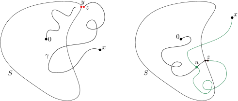
Figure 1: A depiction of Lemma 1.5. On the left we illustrate how we decompose a path $\gamma$ contributing to $G_{\beta}^{\Lambda}(0,x)$. The first edge leaving $S$ is represented in red. On the right we illustrate a configuration in which the portions of $\gamma$ from $0$ to $z$ (in black) and from $z$ to $x$ (in green) interact through an intersection inside $S$. This situation contributes to the error term in (1.20).

Acknowledgements.

Early discussions with Vincent Tassion have been fundamental to the success of this project. We are tremendously thankful to him for these interactions without which the paper would never have existed. We warmly thank Gordon Slade for stimulating discussions and for useful comments. We also thank Gady Kozma, Trishen S. Gunaratnam, Ioan Manolescu, Aman Markar, Christoforos Panagiotis, Alexis Prévost, and Florian Schweiger for many useful comments on an earlier version of this paper. This project has received funding from the Swiss National Science Foundation, the NCCR SwissMAP, and the European Research Council (ERC) under the European Union’s Horizon 2020 research and innovation programme (grant agreement No. 757296). HDC acknowledges the support from the Simons collaboration on localization of waves.

2 Proof of Theorem 1.1

We will use a bootstrap argument (following the original idea from [Sla87]) and prove that an a priori estimate on the two-point function can be improved for sufficiently small $\lambda$. One original feature of our proof is that the key quantities we track in the bootstrap involve the half-space rather than the full-space. This contrasts for instance with lace expansion, in which all arguments require the full-space two-point function.

The idea will be to observe that the two inequalities of Lemma 1.5 provide a good control on $\varphi_{\beta}(\mathbb{H}_{n})$, which can be interpreted as an averaged (or $\ell^{1}$) estimate on the half-space two-point function at distance $n$. The point-wise (or $\ell^{\infty}$) half-space estimate (1.8) will follow from a regularity property which allows to compare two-point functions ending at close points. Finally, we will deduce the full-space estimate from the half-space one.

To implement this scheme, we introduce the following quantity $\beta^{*}$.

Definition 2.1.

Fix $d>4$ and $\lambda\in(0,1)$. Let $C>0$ to be fixed later. Define $\beta^{*}=\beta^{*}(C,\lambda)$ to be the largest real number in $[0,\beta_{c}]$ such that for every $\beta<\beta^{*}$,

$$\varphi_{\beta}(\mathbb{H}_{n}) <1+\frac{1}{2d} \forall n\geq 0, \ell^{1}_{\beta}$$ ()

$$G_{\beta}^{\mathbb{H}_{n}}(0,x) <\frac{C}{n^{d-1}} \forall n\geq 1,\forall x\in\partial\mathbb{H}_{n}. \ell^{\infty}_{\beta}$$ ()

The $\tfrac{1}{2d}$ is quite arbitrary in ($\ell^{1}_{\beta}$). In fact, we could take any number in $(0,\tfrac{1}{2d}]$. Note that $\beta^{*}\geq\tfrac{1}{2d}$ when $C$ exceeds a large enough constant $\mathbf{C}_{\rm RW}=\mathbf{C}_{\rm RW}(d)>0$, as a bound by the corresponding random walk quantities implies that the estimates are true at $\beta=\frac{1}{2d}$.

Our goal is to show that $\beta^{*}$ is in fact equal to $\beta_{c}$ provided that $C$ and $\lambda$ are properly chosen. We proceed in three steps. First, we show that the bound on $\varphi_{\beta}(\mathbb{H}_{n})$ can be improved when $\beta<\beta^{*}$. Second, we control the gradient of the two-point function. Third, we use the fact that the two-point function does not fluctuate too much (thanks to the second point) to obtain an improved $\ell^{\infty}$ estimate. From these improvements, we obtain that $\beta^{*}$ cannot be strictly smaller than $\beta_{c}$, since in this case the improved estimates would remain true for $\beta$ slightly larger than $\beta^{*}$, which would contradict the definition of $\beta^{*}$.

2.1 Improving the bound on $\varphi_{\beta}(\mathbb{H}_{n})$

This section is the crucial step of our strategy: from the bounds ($\ell^{1}_{\beta}$) and ($\ell^{\infty}_{\beta}$), we obtain a bound on $\varphi_{\beta}(\mathbb{H}_{n})$ that involves the parameter $\lambda$. For small $\lambda$, this bound is an improvement on ($\ell^{1}_{\beta}$). Recall that $\mathbf{C}_{\rm RW}$ satisfies the following property: for every $C>\mathbf{C}_{\rm RW}$ and every $\lambda\in(0,1)$, $\beta^{*}(C,\lambda)\geq\tfrac{1}{2d}$.

Proposition 2.2 (Improving the bound on $\varphi_{\beta}(\mathbb{H}_{n})$).

Fix $d>4$ and $C>\mathbf{C}_{\rm RW}$. There exists $K=K(C,d)<\infty$ such that for every $\lambda\in(0,1)$, every $\beta<\beta^{*}(C,\lambda)$, and every $n\geq 0$,

$$\varphi_{\beta}(\mathbb{H}_{n}) <1+K\lambda,$$ (2.1)

$$\sup\{\varphi_{\beta}(B):B\in\mathcal{B}\} \leq 1+K\lambda,$$ (2.2)

where $\mathcal{B}$ is the set of blocks, that is $\mathcal{B}:=\{(\prod_{i=1}^{d}[a_{i},b_{i}])\cap\mathbb{Z}^{d}:\forall 1\leq i\leq d,a_{i}\leq 0\leq b_{i}\}$.

In the rest of Section 2.1, we fix $\lambda\in(0,1)$ and drop it from the notations. We start with a number of elementary bounds on the two-point function in the bulk and in half-space induced by the assumption that $\beta<\beta^{*}$.

Lemma 2.3.

Fix $d>4$ and $C>0$. For every $\beta<\beta^{*}(C)$,

$$G_{\beta}(0,x) \leq\frac{2C}{|x|^{d-2}}\qquad \forall x\in\mathbb{Z}^{d}\setminus\{0\},$$ (2.3)

$$G_{\beta}^{\mathbb{H}_{n}}(0,x) \leq\frac{2C(k+1)}{(n-k)^{d-1}}\qquad \forall x\in\partial\mathbb{H}_{n-k}\text{ with }1\leq k<n,$$ (2.4)

$$\sum_{x\in\partial\mathbb{H}_{n-k}}G_{\beta}^{\mathbb{H}_{n}}(0,x)\beta \leq 4(k+1)\qquad \text{ with }n,k\geq 0.$$ (2.5)

Proof.

Let us start with (2.3). Without loss of generality, assume that $x_{1}=|x|$. Consider a path from $0$ to $x$. If the path is not included in $\mathbb{H}$, decompose it according to the first edge $yz$ where $z$ is a left-most point; see Figure 2. This yields

$$G_{\beta}(0,x) \stackrel{{\scriptstyle\phantom{\eqref{eq:H_beta-''}}}}{{\leq}}G^{\mathbb{H}}_{\beta}(0,x)+\sum_{n\geq 0}\sum_{\begin{subarray}{c}y\in\mathbb{H}_{n}\\ z\notin\mathbb{H}_{n}\\ y\sim z\end{subarray}}G_{\beta}^{\mathbb{H}_{n}}(0,y)\beta G_{\beta}^{\mathbb{H}_{n+1}}(z,x)$$ (2.6)

$$\stackrel{{\scriptstyle\eqref{eq:H_beta-''}}}{{\leq}}\frac{C}{|x|^{d-1}}+\sum_{n\geq 0}\varphi_{\beta}(\mathbb{H}_{n})\frac{C}{(|x|+n+1)^{d-1}}\stackrel{{\scriptstyle\eqref{eq:H_beta}}}{{\leq}}\frac{C(1+\tfrac{1+(2d)^{-1}}{d-2})}{|x|^{d-2}}\leq\frac{2C}{|x|^{d-2}},$$ (2.7)

where in the penultimate inequality, we used that $\sum_{n\geq\alpha}\tfrac{1}{(n+1)^{d-1}}\leq\tfrac{1}{(d-2)\alpha^{d-2}}$ for every $\alpha\geq 1$.

We turn to (2.4). Let $1\leq k<n$. Pick $x\in\partial\mathbb{H}_{n-k}$. To bound $G_{\beta}^{\mathbb{H}_{n}}(x,0)=G_{\beta}^{\mathbb{H}_{n}}(0,x)$, decompose the path from $x$ to 0 in the same fashion as above (see Figure 2) to get

$$G^{\mathbb{H}_{n}}_{\beta}(x,0) \stackrel{{\scriptstyle\phantom{\eqref{eq:H_beta-''}}}}{{\leq}}G^{\mathbb{H}_{n-k}}_{\beta}(x,0)+\sum_{j=1}^{k}\sum_{\begin{subarray}{c}y\in\mathbb{H}_{n-j}\\ z\notin\mathbb{H}_{n-j}\\ y\sim z\end{subarray}}G_{\beta}^{\mathbb{H}_{n-j}}(x,y)\beta G_{\beta}^{\mathbb{H}_{n-j+1}}(z,0)$$ (2.8)

$$\stackrel{{\scriptstyle\eqref{eq:H_beta-''}}}{{\leq}}\frac{C}{(n-k)^{d-1}}+\sum_{j=1}^{k}\Big{(}\sum_{\begin{subarray}{c}y\in\mathbb{H}_{n-j}\\ z\notin\mathbb{H}_{n-j}\\ y\sim z\end{subarray}}G_{\beta}^{\mathbb{H}_{n-j}}(x,y)\beta\Big{)}\frac{C}{(n-j+1)^{d-1}}$$ (2.9)

$$\stackrel{{\scriptstyle\eqref{eq:H_beta}}}{{\leq}}\frac{C(1+(2d)^{-1})(k+1)}{(n-k)^{d-1}}\leq\frac{2C(k+1)}{(n-k)^{d-1}}.$$ (2.10)

For the proof of (2.5), consider the same decomposition (2.8) and sum it over $x\in\partial\mathbb{H}_{n-k}$, then use ($\ell^{1}_{\beta}$) twice instead of ($\ell^{1}_{\beta}$) and ($\ell^{\infty}_{\beta}$). When $1\leq k\leq n$, this gives

$$\sum_{x\in\partial\mathbb{H}_{n-k}}G_{\beta}^{\mathbb{H}_{n}}(0,x) \stackrel{{\scriptstyle\eqref{eq: decomposition at distance k from hyperplane}}}{{\leq}}\frac{\varphi_{\beta}(\mathbb{H}_{n-k})}{\beta}+\sum_{j=1}^{k}\varphi_{\beta}(\mathbb{H}_{k-j})\frac{\varphi_{\beta}(\mathbb{H}_{n-j+1})}{\beta}$$ (2.11)

$$\stackrel{{\scriptstyle\eqref{eq:H_beta}}}{{\leq}}\frac{1}{\beta}\Big{(}(1+(2d)^{-1})+k(1+(2d)^{-1})^{2}\Big{)}\leq\frac{4(k+1)}{\beta}.$$ (2.12)

When $k>n$ we adapt (2.8) and get

$$G_{\beta}^{\mathbb{H}_{n}}(x,0)\leq G_{\beta}^{\mathbb{H}}(x,0)+\sum_{j=1}^{n}\sum_{\begin{subarray}{c}y\in\mathbb{H}_{n-j}\\ z\notin\mathbb{H}_{n-j}\\ y\sim z\end{subarray}}G_{\beta}^{\mathbb{H}_{n-j}}(x,y)\beta G_{\beta}^{\mathbb{H}_{n-j+1}}(z,0).$$ (2.13)

Summing (2.13) over $x\in\partial\mathbb{H}_{n-k}$, we obtain similarly,

$$\sum_{x\in\partial\mathbb{H}_{n-k}}G_{\beta}^{\mathbb{H}_{n}}(0,x)\leq\frac{4(n+1)}{\beta}\leq\frac{4(k+1)}{\beta}.$$ (2.14)

This concludes the proof. ∎

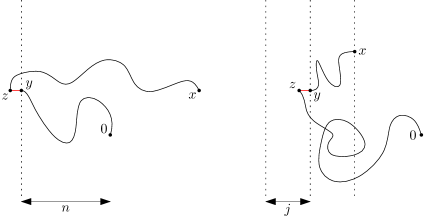
Figure 2: On the left, an illustration of the decomposition of the path used in the proof of (2.3). The red edge $yz$ is the earliest edge satisfying that $z$ is a left-most point of the path. On the right, an illustration of the decomposition of the path used in the proof of (2.4).

We now turn to the estimate of the error amplitude in (1.20) when $\beta<\beta^{*}$.

Lemma 2.4 (Bounding the error amplitude).

Fix $d>4$ and $C>\mathbf{C}_{\rm RW}$. There exists $K=K(C,d)>0$ such that for every $\beta<\beta^{*}(C)$, and every $n\geq 0$,

$$E_{\beta}^{\mathbb{H}_{n},\mathbb{Z}^{d}} \leq K,$$ (2.15)

$$\sup\big{\{}E_{\beta}^{B,\mathbb{Z}^{d}}:B\in\mathcal{B}\} \leq K.$$ (2.16)

Proof.

The second inequality follows from the first one (by changing $K$) since for every $B\in\mathcal{B}$,

$$E_{\beta}^{B,\mathbb{Z}^{d}} \leq 2d\max\big{\{}E_{\beta}^{\mathbb{H}_{k},\mathbb{Z}^{d}}:k\geq 0\}.$$ (2.17)

For the first inequality, we notice that $E_{\beta}^{\mathbb{H}_{n},\mathbb{Z}^{d}}$ is increasing in $\beta$, so that it is sufficient to prove the bound for $\beta\geq\tfrac{1}{4d}$ (recall that since $C>\mathbf{C}_{\rm RW}$, one has $\beta^{*}\geq\tfrac{1}{2d}$). The previous lemma (more specifically (2.3) and (2.5)) and ($\ell^{1}_{\beta}$) give

$$E_{\beta}^{\mathbb{H}_{n},\mathbb{Z}^{d}} =\sum_{k\geq 0}\sum_{u\in\partial\mathbb{H}_{n-k}}\sum_{\begin{subarray}{c}y\in\mathbb{H}_{n}\\ z\notin\mathbb{H}_{n}\\ y\sim z\end{subarray}}G_{\beta}^{\mathbb{H}_{n}}(0,u)G_{\beta}^{\mathbb{H}_{n}}(u,y)\beta G_{\beta}(z,u)$$ (2.18)

$$\leq\sum_{k\geq 0}\Big{(}\sum_{u\in\partial\mathbb{H}_{n-k}}G_{\beta}^{\mathbb{H}_{n}}(0,u)\Big{)}\cdot\Big{(}1+\frac{1}{2d}\Big{)}\cdot\frac{2C}{(k+1)^{d-2}}$$ (2.19)

$$\leq\sum_{k\geq 0}\frac{4(k+1)}{\beta}\cdot\Big{(}1+\frac{1}{2d}\Big{)}\cdot\frac{2C}{(k+1)^{d-2}}$$ (2.20)

which is finite and depends only on $C,d$ as soon as $d>4$ and $\beta\geq\tfrac{1}{4d}$. ∎

We are now in a position to prove Proposition 2.2.

Proof of Proposition 2.2.

Summing (1.20) for $S=\mathbb{H}_{n}$ and $\Lambda=\mathbb{Z}^{d}$ over every $x\in\mathbb{Z}^{d}$ gives

$$\varphi_{\beta}(\mathbb{H}_{n})\chi(\beta)-\lambda\chi(\beta)E_{\beta}^{\mathbb{H}_{n},\mathbb{Z}^{d}}\leq\chi(\beta),$$ (2.21)

where we used that $G^{\mathbb{H}_{n}}_{\beta}(0,x)\geq 0$ for all $x\in\mathbb{Z}^{d}$. Dividing by $\chi(\beta)$ and using Lemma 2.4, we obtain

$$\varphi_{\beta}(\mathbb{H}_{n})\leq 1+\lambda E_{\beta}^{\mathbb{H}_{n},\mathbb{Z}^{d}}\leq 1+K\lambda.$$ (2.22)

The same reasoning, with (1.20) applied to $S=B\in\mathcal{B}$ and $\Lambda=\mathbb{Z}^{d}$ yields

$$\varphi_{\beta}(B)\leq 1+\lambda E_{\beta}^{B,\mathbb{Z}^{d}}\stackrel{{\scriptstyle\eqref{eq:bound error 2 wsaw}}}{{\leq}}1+K\lambda,$$ (2.23)

which concludes the proof. ∎

2.2 Control of the gradient

Proposition 2.2 implies an $\ell^{1}$-type bound on $G_{\beta}^{\mathbb{H}_{n}}$ which involves the quantity $\lambda$ and which is better than ($\ell^{1}_{\beta}$). The following regularity estimate, which will be the goal of this section, will later allow us to convert this $\ell^{1}$ bound into an improved $\ell^{\infty}$ bound.

Proposition 2.5 (Regularity estimate at mesoscopic scales).

Fix $d>4$ and $C>\mathbf{C}_{\rm RW}$. For every $\eta>0$, there exists $\delta=\delta(\eta,d)\in(0,1/2)$ and $\lambda_{0}=\lambda_{0}(\eta,C,d)>0$ such that for every $\lambda<\lambda_{0}$, every $\beta<\beta^{*}(C,\lambda)$, every integer $n$ with $\lfloor\delta n\rfloor\geq 6$, every $\Lambda\supset\Lambda_{3n}$, every $x\notin\Lambda_{3n}$,

$$\max\big{\{}|G_{\beta}^{\Lambda}(u,x)-G_{\beta}^{\Lambda}(v,x)|:u,v\in\Lambda_{\lfloor\delta n\rfloor}\cap 2\mathbb{Z}^{d}\big{\}} \leq\eta\max\big{\{}G_{\beta}^{\Lambda}(w,x):w\in\Lambda_{3n}\big{\}}.$$ (2.24)

Remark 2.6.

We will see later that the assumption $u,v\in 2\mathbb{Z}^{d}$ is not necessary (see Corollary 3.4), but we will not need this stronger result in this section.

We start with a lemma. Let $\Lambda_{n}^{+}:=\{x\in\Lambda_{n}:x_{1}>0\}$ and $H:=\{v\in\mathbb{Z}^{d}:\>v_{1}=0\}$.

Lemma 2.7.

Fix $d>4$ and $C>\mathbf{C}_{\rm RW}$. Assume that $\lambda\leq\tfrac{1}{2dK}$, where $K=K(C,d)$ is given by Proposition 2.2. Let $n\geq 12$. For every $v\in\Lambda_{k}^{+}$ with $6\leq k\leq n/2$ and every $\beta<\beta^{*}(C,\lambda)$,

$$\sum_{\begin{subarray}{c}y\in\Lambda_{n}^{+}\\ z\notin\Lambda_{n}^{+}\cup H\\ y\sim z\end{subarray}}G_{\beta}^{\Lambda_{n}^{+}}(v,y)\beta\leq 4\Big{(}\frac{2k}{n}\Big{)}^{c},$$ (2.25)

where $c:=\tfrac{|\log(1-\tfrac{1}{4d^{2}})|}{2\log 2}$.

Proof.

Define $(n_{\ell})$ by $n_{0}:=n$ and then $n_{\ell+1}:=\lfloor(n_{\ell}-1)/2\rfloor$. We prove by induction that for every $\ell\geq 0$ and $v\in\Lambda_{n_{\ell}}^{+}$,

$$\sum_{\begin{subarray}{c}y\in\Lambda_{n}^{+}\\ z\notin\Lambda_{n}^{+}\cup H\\ y\sim z\end{subarray}}G_{\beta}^{\Lambda_{n}^{+}}(v,y)\beta\leq\Big{(}1-\frac{1}{4d^{2}}\Big{)}^{\ell}\Big{(}1+\frac{1}{2d}\Big{)}.$$ (2.26)

The case $\ell=0$ follows from Proposition 2.2 and from the assumption made on $\lambda$. Let us transfer the estimate from $\ell$ to $\ell+1$. Fix $v\in\Lambda_{n_{\ell+1}}^{+}$. Let $B:=\Lambda_{v_{1}-1}(v)$, which is included in $\Lambda_{n_{\ell}}^{+}$ and has one of its faces at distance $1$ from $H$. By symmetry, we have that

$$\sum_{\begin{subarray}{c}r\in B\\ s\notin B\cup H\\ r\sim s\end{subarray}}G_{\beta}^{B}(v,r)\beta\leq\frac{2d-1}{2d}\varphi_{\beta}(B)\stackrel{{\scriptstyle\eqref{eq:bound varphi box wsaw}}}{{\leq}}\Big{(}1-\frac{1}{2d}\Big{)}(1+\lambda K)\leq\Big{(}1-\frac{1}{2d}\Big{)}\Big{(}1+\frac{1}{2d}\Big{)}=1-\frac{1}{4d^{2}}.$$ (2.27)

Lemma 1.5 (applied to $S=B$ and $\Lambda=\Lambda_{n}^{+}$) and the induction hypothesis imply that

$$\sum_{\begin{subarray}{c}y\in\Lambda_{n}^{+}\\ z\notin\Lambda_{n}^{+}\cup H\\ y\sim z\end{subarray}}G_{\beta}^{\Lambda_{n}^{+}}(v,y)\beta \stackrel{{\scriptstyle\phantom{\eqref{eq:j1}}}}{{\leq}}\sum_{\begin{subarray}{c}y\in\Lambda_{n}^{+}\\ z\notin\Lambda_{n}^{+}\cup H\\ y\sim z\end{subarray}}\Big{(}\sum_{\begin{subarray}{c}r\in B\\ s\notin B\cup H\\ r\sim s\end{subarray}}G_{\beta}^{B}(v,r)\beta G_{\beta}^{\Lambda_{n}^{+}}(s,y)\Big{)}\beta$$ (2.28)

$$\stackrel{{\scriptstyle\phantom{\eqref{eq:j1}}}}{{=}}\sum_{\begin{subarray}{c}r\in B\\ s\notin B\cup H\\ r\sim s\end{subarray}}G_{\beta}^{B}(v,r)\beta\Big{(}\sum_{\begin{subarray}{c}y\in\Lambda_{n}^{+}\\ z\notin\Lambda_{n}^{+}\cup H\\ y\sim z\end{subarray}}G_{\beta}^{\Lambda_{n}^{+}}(s,y)\beta\Big{)}$$ (2.29)

$$\stackrel{{\scriptstyle\phantom{\eqref{eq:j1}}}}{{\leq}}\Big{(}1-\frac{1}{4d^{2}}\Big{)}^{\ell}\Big{(}1+\frac{1}{2d}\Big{)}\sum_{\begin{subarray}{c}r\in B\\ s\notin B\cup H\\ r\sim s\end{subarray}}G_{\beta}^{B}(v,r)\beta$$ (2.30)

$$\stackrel{{\scriptstyle\eqref{eq:j1}}}{{\leq}}\Big{(}1-\frac{1}{4d^{2}}\Big{)}^{\ell+1}\Big{(}1+\frac{1}{2d}\Big{)}.$$ (2.31)

This concludes the proof of the induction. Now, if $k\leq n/2$, one has $k\leq n_{\lfloor\alpha/2\rfloor}$ where $\alpha=\log_{2}(\tfrac{n}{2k})$. Hence, by (2.26), if $v\in\Lambda_{k}^{+}$,

$$\sum_{\begin{subarray}{c}y\in\Lambda_{n}^{+}\\ z\notin\Lambda_{n}^{+}\cup H\\ y\sim z\end{subarray}}G_{\beta}^{\Lambda_{n}^{+}}(v,y)\beta\leq\Big{(}1-\frac{1}{4d^{2}}\Big{)}^{\lfloor\tfrac{1}{2}\log_{2}(\tfrac{n}{2k})\rfloor}\Big{(}1+\frac{1}{2d}\Big{)}\leq\Big{(}\frac{2k}{n}\Big{)}^{c}\Big{(}1+\frac{1}{2d}\Big{)}^{2}\leq 4\Big{(}\frac{2k}{n}\Big{)}^{c},$$ (2.32)

where $c=\tfrac{|\log(1-\tfrac{1}{4d^{2}})|}{2\log 2}$, and where we used that $(1-\tfrac{1}{4d^{2}})^{-1}\leq 1+\tfrac{1}{2d}\leq 2$ for $d\geq 1$. ∎

Proof of Proposition 2.5.

It suffices to prove the statement when $u$ and $v$ differ in one coordinate only as the general case follows by summing increments over coordinates. By rotating and translating, we may consider $u=k{\bf e}_{1}$ and $v=-k{\bf e}_{1}$ belong to $\Lambda_{\lfloor\delta n\rfloor}\cap(2\mathbb{Z}^{d})$ for $\delta$ to be fixed, and later replace the maximum in $\Lambda_{2n}$ by the maximum in $\Lambda_{3n}\supset\Lambda_{2n+\lfloor\delta n\rfloor}$.

Consider the sets $A:=\Lambda_{n}^{+}$ and $B:=-\Lambda_{n}^{+}$. Applying Lemma 1.5 twice as well as Lemma 2.4 gives

$$G_{\beta}^{\Lambda}(u,x) \leq\sum_{\begin{subarray}{c}y\in A\\ z\notin A\\ y\sim z\end{subarray}}G_{\beta}^{A}(u,y)\beta G_{\beta}^{\Lambda}(z,x),$$ (2.33)

$$G_{\beta}^{\Lambda}(v,x) \geq\sum_{\begin{subarray}{c}y\in B\\ z\notin B\\ y\sim z\end{subarray}}G_{\beta}^{B}(v,y)\beta G_{\beta}^{\Lambda}(z,x)-K\lambda\max\{G_{\beta}^{\Lambda}(w,x):w\in B\},$$ (2.34)

where in (2.34) we used that,

$$\sum_{u\in B}E^{B,\Lambda}_{\beta}(u)G_{\beta}^{\Lambda}(u,x) \stackrel{{\scriptstyle\phantom{\eqref{eq:bound error 2 wsaw}}}}{{\leq}}E_{\beta}^{B,\Lambda}\cdot\max\{G_{\beta}^{\Lambda}(w,x):w\in B\}$$ (2.35)

$$\stackrel{{\scriptstyle\eqref{eq:bound error 2 wsaw}}}{{\leq}}K\max\{G_{\beta}^{\Lambda}(w,x):w\in B\}.$$ (2.36)

We take the difference and use that when $z\in H$, the corresponding terms in the two sums cancel each other, see Figure 3. Assume that $\lambda\leq\tfrac{1}{2dK}$ and $\lfloor\delta n\rfloor\geq 6$. Lemma 2.7 applied to $k=\lfloor\delta n\rfloor$ and $n$ gives

$$G_{\beta}^{\Lambda}(u,x)-G_{\beta}^{\Lambda}(v,x) \leq\sum_{\begin{subarray}{c}y\in A\\ z\notin A\cup H\\ y\sim z\end{subarray}}G_{\beta}^{A}(u,y)\beta G_{\beta}^{\Lambda}(z,x)+K\lambda\max\{G_{\beta}^{\Lambda}(w,x):w\in B\}$$ (2.37)

$$\leq\Big{(}4(2\delta)^{c}+K\lambda\Big{)}\max\{G_{\beta}^{\Lambda}(w,x):w\in\Lambda_{2n}\}.$$ (2.38)

The proof follows by choosing $\delta=\delta(\eta,d)>0$ and $\lambda_{0}=\lambda_{0}(\eta,C,d)>0$ small enough. ∎

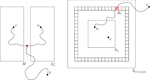
Figure 3: On the left, an illustration of the pairing used in the proof of Proposition 2.5. Since $u$ (resp. $v$) is close to $H$, a path started from $u$ will most likely touch $H$ if it exits $\Lambda_{n}^{+}$. On the right, an illustration of the proof of Proposition 3.2.

2.3 Wrapping up the proof of Theorem 1.1

We start by showing how to use Proposition 2.5 to turn the improved $\ell^{1}$ estimate of $G^{\mathbb{H}_{n}}_{\beta}$ given by Proposition 2.2 into an improved $\ell^{\infty}$ bound.

Proposition 2.8 (Improving the bound on $G_{\beta}^{\mathbb{H}_{n}}$).

Fix $d>4$. There exist $C=C(d),\lambda_{0}=\lambda_{0}(d)>0$ such that, for every $\lambda<\lambda_{0}$, and every $\beta<\beta^{*}(C,\lambda)$,

$$G_{\beta}^{\mathbb{H}_{n}}(0,x)\leq\frac{C}{2n^{d-1}}\qquad\forall n\geq 1,\forall x\in\partial\mathbb{H}_{n}.$$ (2.39)

Proof.

Let $\eta>0$ and $C>\mathbf{C}_{\rm RW}$ to be fixed. By monotonicity of $G_{\beta}^{\mathbb{H}_{n}}(0,x)$ in $\beta$, it suffices to prove the result for $\beta\in[\tfrac{1}{4d},\beta^{*})$. Let $\delta=\delta(\eta,d)$ and $\lambda_{0}=\lambda_{0}(\eta,C,d)$ be provided by Proposition 2.5. Assume first that $\tfrac{\delta n}{6}$ is an integer (otherwise simply round the number) and that $\tfrac{\delta n}{6}\geq 6$. Set

$$V_{n}=V_{n}(\delta):=\Big{\{}x\in\Lambda_{\delta n/6}:x_{1}=0,\>x_{j}\text{ even for }j\geq 2\Big{\}}.$$ (2.40)

Proposition 2.5 applied to $n/6$ gives that for every $\beta<\beta^{*}$, every $x\in\partial\mathbb{H}_{n}$ and $y\in V_{n}$,

$$G_{\beta}^{\mathbb{H}_{n}}(0,x-y) =G_{\beta}^{\mathbb{H}_{n}}(y,x)$$ (2.41)

$$\geq G_{\beta}^{\mathbb{H}_{n}}(0,x)-\eta\max\{G_{\beta}^{\mathbb{H}_{n}}(v,x):v\in\Lambda_{n/2}\}.$$ (2.42)

Fix $x\in\partial\mathbb{H}_{n}$. Averaging the last displayed equation over $y\in V_{n}$ and using that $\beta\geq\tfrac{1}{4d}$ gives

$$\frac{8d}{|V_{n}|}\stackrel{{\scriptstyle\phantom{\eqref{eq:H_beta}}}}{{\geq}}\frac{4d(1+(2d)^{-1})}{|V_{n}|}\stackrel{{\scriptstyle\eqref{eq:H_beta}}}{{\geq}}\frac{\varphi_{\beta}(\mathbb{H}_{n})}{\beta{|V_{n}|}}\geq\frac{1}{|V_{n}|}\sum_{y\in V_{n}}G_{\beta}^{\mathbb{H}_{n}}(0,x-y)\geq G_{\beta}^{\mathbb{H}_{n}}(0,x)-\eta\cdot\frac{C}{(n/2)^{d-1}},$$ (2.43)

where in the last inequality we used ($\ell^{\infty}_{\beta}$) to argue that

$$\max\{G_{\beta}^{\mathbb{H}_{n}}(v,x):v\in\Lambda_{n/2}\}\leq\frac{C}{(n/2)^{d-1}}.$$ (2.44)

If $\eta$ is chosen so that $\eta\leq 1/2^{d+1}$, then $C=C(\delta,d)$ is chosen large enough, we find that

$$\sup_{x\in\partial\mathbb{H}_{n}}G_{\beta}^{\mathbb{H}_{n}}(0,x)\leq\frac{C}{2n^{d-1}}$$ (2.45)

provided $n$ is large enough (i.e. $\tfrac{\delta n}{6}\geq 6$).

To treat the small values of $n$, we observe that for all $n\geq 1$, for all $x\in\partial\mathbb{H}_{n}$, $G_{\beta}^{\mathbb{H}_{n}}(0,x)\leq\varphi_{\beta}(\mathbb{H}_{n})\leq 1+\tfrac{1}{2d}\leq 2$. Thus, if we additionally require that $C\geq 4(36\delta^{-1})^{d-1}$, we ensure that for all $1\leq n\leq 36\delta^{-1}$,

$$\sup_{x\in\partial\mathbb{H}_{n}}G^{\mathbb{H}_{n}}(0,x)\leq\frac{C}{2n^{d-1}}.$$ (2.46)

This concludes the proof. ∎

Proposition 2.9.

Fix $d>4$. There exist $C=C(d),\lambda_{0}=\lambda_{0}(d)>0$, and $K=K(C,d)>0$ such that for every $\lambda<\lambda_{0}$,

$$G_{\beta_{c}}(0,x) \leq\frac{2C}{|x|^{d-2}} \forall x\in\mathbb{Z}^{d}\setminus\{0\},$$ (2.47)

$$G_{\beta_{c}}^{\mathbb{H}}(0,x) \leq\frac{C}{|x_{1}|^{d-1}} \forall x\in\mathbb{H}\setminus\partial\mathbb{H},$$ (2.48)

$$\varphi_{\beta_{c}}(\mathbb{H}_{n}) \leq 1+K\lambda \forall n\geq 0,$$ (2.49)

$$\sup\{\varphi_{\beta_{c}}(B):B\in\mathcal{B}\} \leq 1+K\lambda,$$ (2.50)

$$E^{\mathbb{H}_{n},\mathbb{Z}^{d}}_{\beta_{c}} \leq K \forall n\geq 0,$$ (2.51)

$$\sup\big{\{}E^{B,\mathbb{Z}^{d}}_{\beta_{c}}:B\in\mathcal{B}\big{\}} \leq K.$$ (2.52)

Proof.

We let $C,\lambda_{0}$ be given by Proposition 2.8. This choice gives (still by Proposition 2.8) that for every $\lambda<\lambda_{0}$ and every $\beta<\beta^{*}(C,\lambda)$,

$$G_{\beta}^{\mathbb{H}_{n}}(0,x)\leq\frac{C}{2n^{d-1}}\qquad\forall n\geq 1,\forall x\in\partial\mathbb{H}_{n}.$$ (2.53)

Let $K=K(C,d)$ be given by Proposition 2.2. We potentially decrease the value of $\lambda_{0}$ (which does not affect the value of $C$) and require that $K\lambda_{0}<\tfrac{1}{4d}$. Proposition 2.2 implies that for every $\lambda<\lambda_{0}$ and every $\beta<\beta^{*}(C,\lambda)$,

$$\varphi_{\beta}(\mathbb{H}_{n})\leq 1+K\lambda\leq 1+\frac{1}{4d}\qquad\forall n\geq 0.$$ (2.54)

The monotone convergence theorem implies that (2.53)–(2.54) still hold at $\beta^{*}$. We will use (2.53)–(2.54) to prove that for this choice of $C,\lambda_{0}$: for all $\lambda<\lambda_{0}$,

$$\beta^{*}=\beta^{*}(C,\lambda)=\beta_{c}.$$ (2.55)

Let $\lambda<\lambda_{0}$. Assume by contradiction that $\beta^{*}=\beta^{*}(C,\lambda)<\beta_{c}$. Exponential decay of the two-point function below $\beta_{c}$ implies that for every $\beta<\beta_{c}$, there exists $c(\beta),C(\beta)>0$ such that for all $n\geq 1$, for all $x\in\partial\mathbb{H}_{n}$,

$$G^{\mathbb{H}_{n}}_{\beta}(0,x)\leq C(\beta)e^{-c(\beta)|x|}.$$ (2.56)

Let $\beta^{**}$ be any number in $(\beta^{*},\beta_{c})$. By monotonicity of all the quantities in $\beta$ and (2.56), there exists $N\geq 0$ such that for every $\beta<\beta^{**}$, one has

$$\varphi_{\beta}(\mathbb{H}_{n})<1+\frac{1}{2d}\quad\forall n\geq N,\qquad G_{\beta}^{\mathbb{H}_{n}}(0,x)<\frac{C}{n^{d-1}}\quad\forall n\geq 1,\forall x\in\partial\mathbb{H}_{n}\setminus\Lambda_{N}.$$ (2.57)

Now, (2.57), the validity of (2.53)–(2.54) at $\beta^{*}$, together with the continuity (below $\beta_{c}$) of the maps $\beta\mapsto\max\{\varphi_{\beta}(\mathbb{H}_{n}):0\leq n\leq N-1\}$ and $\beta\mapsto\max\{G_{\beta}^{\mathbb{H}_{n}}(0,x):x\in\Lambda_{N}\cap\partial\mathbb{H}_{n},\>n\geq 1\}$ yield the existence of $\beta\in(\beta^{*},\beta^{**})$ such that

$$\varphi_{\beta}(\mathbb{H}_{n})<1+\frac{1}{2d}\quad\forall n\geq 0,\qquad G_{\beta}^{\mathbb{H}_{n}}(0,x)<\frac{C}{n^{d-1}}\qquad\forall n\geq 1,\forall x\in\partial\mathbb{H}_{n}.$$ (2.58)

This clearly contradicts the definition of $\beta^{*}$ and therefore implies that $\beta^{*}=\beta_{c}$.

For the proofs of (2.47)–(2.52), we use Lemmata 2.3–2.4 and Proposition 2.2 to show that the bounds hold for $\beta<\beta_{c}$. We extend these bounds at $\beta_{c}$ using once again the monotone convergence theorem. ∎

Remark 2.10.

The bound $2d\beta_{c}=\varphi_{\beta_{c}}(\{0\})\leq 1+K\lambda$ gives $\beta_{c}\leq\tfrac{1}{2d}(1+K\lambda)$, which complements the bound $\beta_{c}\geq\tfrac{1}{2d}$.

We are now in a position to prove Theorem 1.1.

Proof of Theorem 1.1.

Let $C,\lambda_{0}$ be given by Proposition 2.9 and let $\lambda<\lambda_{0}$. Let $A=A(d)\geq 1$ be such that

$$t^{d-1}\leq Ae^{t}\qquad\forall t\geq 1.$$ (2.59)

Proof of (1.7).

First, if $\beta\leq\beta_{c}$, Proposition 2.9 implies that for $x\in\mathbb{Z}^{d}\setminus\{0\}$ with $|x|\leq L_{\beta}$,

$$G_{\beta}(0,x)\leq\frac{2C}{|x|^{d-2}}\leq\frac{2e^{2}C}{|x|^{d-2}}e^{-2|x|/L_{\beta}}.$$ (2.60)

We now turn to the case of $\beta<\beta_{c}$ and $|x|>L_{\beta}$ (recall that $L_{\beta_{c}}=\infty$). Iterating (1.19) $k:=\lfloor|x|/L_{\beta}\rfloor-1$ times with $S$ being translates of $\Lambda_{L_{\beta}}$ and $\Lambda=\mathbb{Z}^{d}$, we get that

$$G_{\beta}(0,x) \stackrel{{\scriptstyle\phantom{\eqref{eq:upper bound below L}}}}{{\leq}}\varphi_{\beta}(\Lambda_{L_{\beta}})^{k}\max\big{\{}G_{\beta}(y,x):y\notin\Lambda_{L_{\beta}}(x)\big{\}}$$ (2.61)

$$\stackrel{{\scriptstyle\eqref{eq:upper bound below L}}}{{\leq}}e^{-2k}\frac{2C}{L_{\beta}^{d-2}}\stackrel{{\scriptstyle\phantom{\eqref{eq:upper bound below L}}}}{{\leq}}\frac{2e^{4}C}{L_{\beta}^{d-2}}e^{-2|x|/L_{\beta}}\stackrel{{\scriptstyle\eqref{eq:def A wsaw}}}{{\leq}}\frac{2e^{4}AC}{|x|^{d-2}}e^{-|x|/L_{\beta}}.$$ (2.62)

Proof of (1.8).

Again, if $\beta\leq\beta_{c}$, Proposition 2.9 implies that for $x\in\mathbb{H}$ with $0<x_{1}\leq L_{\beta}$,

$$G_{\beta}^{\mathbb{H}}(0,x)\leq\frac{C}{|x_{1}|^{d-1}}\leq\frac{e^{2}C}{|x_{1}|^{d-1}}e^{-2|x_{1}|/L_{\beta}}.$$ (2.63)

Turning to the case $\beta<\beta_{c}$ and $|x_{1}|>L_{\beta}$, iterating (1.19) $\ell:=\lfloor|x_{1}|/L_{\beta}\rfloor-1$ times with $S$ being translates of $\Lambda_{L_{\beta}}$ (starting with $\Lambda_{L_{\beta}}(x)$) and $\Lambda=\mathbb{H}$, we obtain

$$G_{\beta}^{\mathbb{H}}(0,x)=G_{\beta}^{\mathbb{H}}(x,0)\leq\varphi_{\beta}(\Lambda_{L_{\beta}})^{\ell}\max\{G_{\beta}^{\mathbb{H}}(0,y):y_{1}>L_{\beta}\} \stackrel{{\scriptstyle\eqref{eq:upper half-spacebound below L}}}{{\leq}}\frac{e^{4}C}{L_{\beta}^{d-1}}e^{-2|x_{1}|/L_{\beta}}$$ (2.64)

$$\stackrel{{\scriptstyle\eqref{eq:def A wsaw}}}{{\leq}}\frac{e^{4}AC}{|x_{1}|^{d-1}}e^{-|x_{1}|/L_{\beta}}$$ (2.65)

Gathering (2.60), (2.62), (2.63), and (2.65), we obtained: for all $\beta\leq\beta_{c}$, for all $x\in\mathbb{Z}^{d}\setminus\{0\}$,

$$G_{\beta}(0,x) \leq\frac{2e^{4}AC}{|x|^{d-2}}\exp(-|x|/L_{\beta}),$$ (2.66)

$$G_{\beta}^{\mathbb{H}}(0,x) \leq\frac{2e^{4}AC}{|x_{1}|^{d-1}}\exp(-|x_{1}|/L_{\beta}).$$ (2.67)

This concludes the proof. ∎

3 Proof of Theorem 1.2

For $\varepsilon\in(0,1)$, introduce the quantity

$$L_{\beta}(\varepsilon):=\inf\{k\geq 1:\varphi_{\beta}(\Lambda_{k})\leq 1-\varepsilon\}.$$ (3.1)

This new correlation length only differs from $L_{\beta}$ by a constant, as stated in the next lemma, but it will be more convenient for the rest of the proof.

Lemma 3.1 (Comparison between $L_{\beta}$ and $L_{\beta}(\varepsilon)$).

Fix $d>4$ and $\varepsilon\in(0,1-e^{-2})$. Let $\lambda_{0}$ be given by Proposition 2.9. There exists $C(\varepsilon,\lambda_{0},d)\in(0,\infty)$ such that, for every $\lambda<\lambda_{0}$, and every $\beta<\beta_{c}$,

$$L_{\beta}(\varepsilon)\leq L_{\beta}\leq C(\varepsilon,\lambda_{0})L_{\beta}(\varepsilon).$$ (3.2)

Proof.

The first inequality is clear. We turn to the second one. Assume that $L_{\beta}-1\geq k(L_{\beta}(\varepsilon)+1)$. Similarly to (2.61), if we iterate (1.19) $k$ times with $S$ being translates of $\Lambda_{L_{\beta}(\varepsilon)}$ and $\Lambda=\Lambda_{L_{\beta}-1}$, we obtain that: for every $x\in\partial\Lambda_{L_{\beta}-1}$,

$$G_{\beta}^{\Lambda}(0,x)\beta\leq\sum_{\begin{subarray}{c}u_{1}\in\Lambda_{L_{\beta}(\varepsilon)}\\ v_{1}\notin\Lambda_{L_{\beta}(\varepsilon)}\\ u_{1}\sim v_{1}\end{subarray}}G_{\beta}^{\Lambda}(0,u_{1})\beta\ldots\sum_{\begin{subarray}{c}u_{k}\in\Lambda_{L_{\beta}(\varepsilon)}(v_{k-1})\\ v_{k}\notin\Lambda_{L_{\beta}(\varepsilon)}(v_{k-1})\\ u_{k}\sim v_{k}\end{subarray}}G_{\beta}^{\Lambda}(v_{k-1},u_{k})\beta G_{\beta}^{\Lambda}(v_{k},x)\beta.$$ (3.3)

Summing the above displayed equation over $x\in\partial\Lambda_{L_{\beta}-1}$ and $y\sim x$ with $y\notin\Lambda_{L_{\beta}-1}$ gives

$$\frac{1}{e^{2}}\leq\varphi_{\beta}(\Lambda_{L_{\beta}-1})\leq\varphi_{\beta}(\Lambda_{L_{\beta}(\varepsilon)})^{k}\max\{\varphi_{\beta}(\Lambda_{L_{\beta}-1}(x)):x\in\Lambda_{L_{\beta}-1}\}\leq(1-\varepsilon)^{k}(1+K\lambda),$$ (3.4)

where $K$ is given by Proposition 2.9. As a consequence, there exists $C(\varepsilon,\lambda_{0},d)<\infty$ such that $L_{\beta}\leq C(\varepsilon,\lambda_{0},d)L_{\beta}(\varepsilon)$. ∎

Note that the assumption $n\leq L_{\beta}(\varepsilon)-1$ implies an $\ell^{1}$-type lower bound on the half-space two-point function (see (3.28)). The core of this section will be to turn this estimate into a point-wise estimate for the half-space two-point function. The corresponding lower bound for the full-space two-point function will follow readily. The proof is organised in two steps: we begin by proving a regularity estimate, and then we use it to get the theorem.

3.1 A Harnack-type estimate

We start with another regularity estimate relating the minimum to the maximum of the two-point function in a domain.

Proposition 3.2 (Harnack-type estimate at macroscopic scales).

Fix $d>4$ and $\alpha>0$. There exists $C_{\rm RW}=C_{\rm RW}(\alpha,d)>0$ and for every $\eta>0$, there exist $\lambda_{0}=\lambda_{0}(\eta,\alpha,d)$, $\varepsilon_{0}=\varepsilon_{0}(\eta,d)>0$ small enough and $N_{0}=N_{0}(\eta,\alpha,d)$ large enough such that the following holds. For every $\lambda<\lambda_{0}$, every $\varepsilon<\varepsilon_{0}$, every $N_{0}\leq n\leq 6L_{\beta}(\varepsilon)$, every $\tfrac{1}{2d}\leq\beta\leq\beta_{c}$, and every $x\notin\Lambda_{(1+\alpha)n}\subset\Lambda$,

$$\max\{G_{\beta}^{\Lambda}(u,x):u\in\Lambda_{n}\} \leq C_{\rm RW}\min\{G_{\beta}^{\Lambda}(u,x):u\in\Lambda_{n}\}+\eta\max\{G_{\beta}^{\Lambda}(u,x):u\in\Lambda_{(1+\alpha)n}\}.$$ (3.5)

We will derive Proposition 3.2 using classical random walk estimates. We start with a lemma which is useful to go around the parity assumption in Proposition 2.5.

Lemma 3.3.

Fix $d>4$ and $\eta>0$. There exists $\lambda_{0}>0$ such that the following holds. For every $\ell\geq 1$, there exists $L=L(\eta,\ell,d)\geq\ell$ such that for every $\lambda<\lambda_{0}$, every $\tfrac{1}{2d}\leq\beta\leq\beta_{c}$, every set $\Lambda\supset\Lambda_{L}$, and every $x\notin\Lambda_{L}$,

$$\max\big{\{}|G_{\beta}^{\Lambda}(u,x)-G_{\beta}^{\Lambda}(v,x)|:u,v\in\Lambda_{\ell}\big{\}}\leq\eta\max\{G_{\beta}^{\Lambda}(w,x):w\in\Lambda_{L}\}.$$ (3.6)

Proof.

Fix $\eta>0$. Consider the simple random walk $(X_{n})$ defined by

$$\mathbb{P}_{u}[X_{1}=v]:=\tfrac{1}{2d}\mathds{1}_{v\sim u}.$$ (3.7)

Let $\tau$ be the hitting time of $\mathbb{Z}^{d}\setminus\Lambda_{L-1}$. We will use two a priori estimates on the random walk and the stopping time that can be easily obtained from classical random walk analysis (see [LL10]): for every $\ell>0$, there exist $C_{\rm RW}=C_{\rm RW}(d)$ and $L=L(\eta,\ell,d)$ such that for some $\varepsilon=\varepsilon(\eta,\ell,L,d)>0$ and every $\varphi\in[1-\varepsilon,1+\varepsilon]$,

$$\mathbb{E}_{u}\Big{[}\sum_{s=0}^{\tau}\varphi^{s}\Big{]} \leq C_{\rm RW} \forall u\in\Lambda_{\ell},$$ (3.8)

$$\mathbb{E}_{u}[\varphi^{\tau}\mathds{1}_{X_{\tau}=z}] \leq(1+\eta)\mathbb{E}_{v}[\varphi^{\tau}\mathds{1}_{X_{\tau}=z}] \forall u,v\in\Lambda_{\ell},\forall z\in\partial\Lambda_{L}.$$ (3.9)

From now on, we let $\lambda_{0}$ small enough be given by Proposition 2.9 and (to the cost of diminishing $\lambda_{0}$) we additionally require that $K\lambda_{0}\leq\varepsilon$ where $K$ is given by the same proposition. Let $\lambda<\lambda_{0}$ and $\beta\leq\beta_{c}$. By the assumption $\beta\geq\tfrac{1}{2d}$ and Proposition 2.9, we find

$$1\leq 2d\beta=\varphi_{\beta}(\{0\})\leq 1+K\lambda\leq 1+\varepsilon.$$ (3.10)

Below, introduce the shorthand notation $\varphi:=\varphi_{\beta}(\{0\})$. We let $u,v\in\Lambda_{\ell}$ and $x\notin\Lambda_{L}$. Iterating the two bounds of Lemma 1.5 (with $S$ a singleton) until time $\tau$ and using Lemma 2.4 gives

$$G_{\beta}^{\Lambda}(u,x) \stackrel{{\scriptstyle\eqref{eq:SL}}}{{\leq}}\mathbb{E}_{u}[\varphi^{\tau}G_{\beta}^{\Lambda}(X_{\tau},x)],$$ (3.11)

$$G_{\beta}^{\Lambda}(v,x) \stackrel{{\scriptstyle\eqref{eq:reversed SL}}}{{\geq}}\mathbb{E}_{v}[\varphi^{\tau}G_{\beta}^{\Lambda}(X_{\tau},x)]-K\lambda\,\mathbb{E}_{v}\Big{[}\sum_{s=0}^{\tau}\varphi^{s}\Big{]}\max\{G_{\beta}^{\Lambda}(w,x):w\in\Lambda_{L}\}$$ (3.12)

$$\stackrel{{\scriptstyle\ \eqref{eq:hba1}}}{{\geq}}\mathbb{E}_{v}[\varphi^{\tau}G_{\beta}^{\Lambda}(X_{\tau},x)]-K\lambda C_{\rm RW}\max\{G_{\beta}^{\Lambda}(w,x):w\in\Lambda_{L}\}.$$ (3.13)

Taking the difference of (3.11) and (3.13) gives

$$G_{\beta}^{\Lambda}(u,x) -G_{\beta}^{\Lambda}(v,x)$$ (3.14)

$$\stackrel{{\scriptstyle\phantom{\eqref{eq:hca1}}}}{{\leq}}\mathbb{E}_{u}[\varphi^{\tau}G_{\beta}^{\Lambda}(X_{\tau},x)]-\mathbb{E}_{v}[\varphi^{\tau}G_{\beta}^{\Lambda}(X_{\tau},x)]+C_{\rm RW}K\lambda\max\{G_{\beta}^{\Lambda}(w,x):w\in\Lambda_{L}\}$$ (3.15)

$$\stackrel{{\scriptstyle\eqref{eq:hca1}}}{{\leq}}\eta\mathbb{E}_{v}[\varphi^{\tau}G_{\beta}^{\Lambda}(X_{\tau},x)]+C_{\rm RW}K\lambda\max\{G_{\beta}^{\Lambda}(w,x):w\in\Lambda_{L}\}$$ (3.16)

$$\stackrel{{\scriptstyle\eqref{eq:hda}}}{{\leq}}\eta G_{\beta}^{\Lambda}(v,x)+C_{\rm RW}K\lambda(1+\eta)\max\{G_{\beta}^{\Lambda}(w,x):w\in\Lambda_{L}\}.$$ (3.17)

The proof follows by choosing $\lambda_{0}$ even smaller. ∎

Corollary 3.4 (Regularity estimate at mesoscopic scales without the parity assumption).

Fix $d>4$. For every $\eta>0$, there exist $\delta=\delta(\eta,d)\in(0,1/2)$, $\lambda_{0}=\lambda_{0}(\eta,d)>0$, and $L=L(\eta,d)>0$ such that for every $\lambda<\lambda_{0}$, every $\beta\leq\beta_{c}$, every $n\geq L$, every $\Lambda\supset\Lambda_{3n}$, every $x\notin\Lambda_{3n}$,

$$\max\big{\{}|G_{\beta}^{\Lambda}(u,x)-G_{\beta}^{\Lambda}(v,x)|:u,v\in\Lambda_{\lfloor\delta n\rfloor}\big{\}} \leq\eta\max\big{\{}G_{\beta}^{\Lambda}(w,x):w\in\Lambda_{3n}\big{\}}.$$ (3.18)

Proof.

Take $\lambda_{0}$ small enough such that Proposition 2.9 and Lemma 3.3 hold. By continuity, it is sufficient to prove the result for $\beta<\beta_{c}$. The proof follows from applying Proposition 2.5 with $\eta/2$ and Lemma 3.3 with $\eta/2$ and $\ell=1$. ∎

We now turn to the proof of Proposition 3.2. The idea of the proof is the same as in Lemma 3.3, except we introduce a well-chosen rescaled random walk to replace the simple random walk.

Proof of Proposition 3.2.

Fix $M:=\lfloor\alpha n/6\rfloor$. Set $m:=\lfloor\delta M\rfloor$, where $\delta=\delta(\eta,A,d)$ is chosen in such a way that Corollary 3.4 is valid with $\eta/A$ where $A>0$ will be taken large enough below. Also, assume that $n$ is large enough so that $m\geq L$ where $L$ is again provided by Corollary 3.4 (this means $n\geq 6\alpha^{-1}\delta^{-1}L$). Let $B_{1},\dots,B_{s}$ be boxes of size $m$ that are disjoint and covering the annulus $\Lambda_{n+M+m}\setminus\Lambda_{n+M}$, see Figure 3. Consider the random walk $(X_{n}^{\prime})$ defined by

$$\mathbb{P}_{u}^{\prime}[X_{1}^{\prime}=v]:=\frac{\mathds{1}_{v\notin\Lambda_{m}(u)}}{\varphi_{\beta}(\Lambda_{m})}\sum_{\begin{subarray}{c}w\in\Lambda_{m}(u)\\ w\sim v\end{subarray}}G_{\beta}^{\Lambda_{m}(u)}(u,w)\beta.$$ (3.19)

Let $\tau$ be the hitting time of $\mathbb{Z}^{d}\setminus\Lambda_{n+M}$. We will use two a priori estimates on the random walk and the stopping time $\tau$, that can be easily obtained from classical random walk analysis (see [LL10]) : there exists a constant $C_{\rm RW}=C_{\rm RW}(\alpha,d)$ (note that it does not depend on $m$) such that for $\varepsilon=\varepsilon(\alpha,\eta,d)>0$ small enough and every $\varphi\in[1-\varepsilon,1+\varepsilon]$,

$$\mathbb{E}_{u}^{\prime}\Big{[}\sum_{s=0}^{\tau}\varphi^{s}\Big{]} \leq C_{\rm RW} \forall u\in\Lambda_{n},$$ (3.20)

$$\mathbb{E}_{u}^{\prime}[\varphi^{\tau}\mathds{1}_{X^{\prime}_{\tau}\in B_{i}}] \leq C_{\rm RW}\mathbb{E}_{v}^{\prime}[\varphi^{\tau}\mathds{1}_{X^{\prime}_{\tau}\in B_{i}}] \forall u,v\in\Lambda_{n},\forall i\leq s.$$ (3.21)

We let $\lambda_{0}$ small enough be given by Proposition 2.9 and (to the cost of diminishing $\lambda_{0}$) we additionally require that $K\lambda_{0}\leq\varepsilon$ where $K$ is given by the same proposition. Also, consider $u,v\in\Lambda_{n}$. By the assumption $6m<n\leq 6L_{\beta}(\varepsilon)$ and Proposition 2.9, we find

$$1-\varepsilon\leq\varphi_{\beta}(\Lambda_{m})\leq 1+K\lambda\leq 1+\varepsilon.$$ (3.22)

Corollary 3.4 gives that for every $i\leq s$,

$$\mathbb{E}_{u}^{\prime}[\varphi^{\tau}\mathds{1}_{X^{\prime}_{\tau}\in B_{i}}G_{\beta}^{\Lambda}(X_{\tau},x)] \leq\mathbb{E}_{u}^{\prime}[\varphi^{\tau}\mathds{1}_{X^{\prime}_{\tau}\in B_{i}}]\min\{G_{\beta}^{\Lambda}(w,x):w\in B_{i}\}$$

$$\quad+\frac{\eta}{A}\mathbb{E}_{u}^{\prime}[\varphi^{\tau}\mathds{1}_{X^{\prime}_{\tau}\in B_{i}}]\max\{G_{\beta}^{\Lambda}(w,x):w\in\Lambda_{n+4M+m}\},$$ (3.23)

where we used that $B_{i}+\Lambda_{3M}\subset\Lambda_{n+4M+m}$. Moreover, by (3.21),

$$\mathbb{E}_{u}^{\prime}[\varphi^{\tau}\mathds{1}_{X^{\prime}_{\tau}\in B_{i}}]\min\{G_{\beta}^{\Lambda}(w,x):w\in B_{i}\}\leq C_{\rm RW}\mathbb{E}_{v}^{\prime}[\varphi^{\tau}\mathds{1}_{X^{\prime}_{\tau}\in B_{i}}G_{\beta}^{\Lambda}(X_{\tau},x)].$$ (3.24)

Since $n+4M+m\leq(1+\alpha)n$, the end of the proof follows the same lines as in Lemma 3.3: iterating this time (1.19) and (1.20) with $S$ being the box of size $m$ until the stopping time $\tau$, and using (3.20),

$$G_{\beta}^{\Lambda}(u,x)\leq C_{\rm RW}G_{\beta}^{\Lambda}(v,x)+C_{\rm RW}\Big{(}K\lambda+\frac{\eta}{A}\Big{)}\max\{G_{\beta}^{\Lambda}(w,x):w\in\Lambda_{(1+\alpha)n}\}.$$ (3.25)

The proof follows from fixing $A=2C_{\rm RW}$, choosing $\lambda_{0}$ small enough so that $C_{\rm RW}K\lambda_{0}\leq\eta/2$, and setting $N_{0}:=6\alpha^{-1}\delta^{-1}L$. ∎

3.2 Conclusion

We start by lower bounding the half-space two-point function at scale below $6L_{\beta}(\varepsilon)$ (for some technical reasons we will need a multiple of $L_{\beta}(\varepsilon)$ later). Let

$$A_{n}:=\{x\in\mathbb{Z}^{d}:x_{1}=|x|=n\}.$$ (3.26)

Lemma 3.5.

Fix $d>4$. There exist $c,\varepsilon_{0},\lambda_{0}>0$ such that for every $\lambda<\lambda_{0}$, every $\varepsilon<\varepsilon_{0}$, every $\tfrac{1}{2d}\leq\beta\leq\beta_{c}$, and every $x\in\mathbb{H}$ with $x_{1}=|x|\leq 6L_{\beta}(\varepsilon)$,

$$G_{\beta}^{\mathbb{H}}(0,x)\geq\frac{c}{|x|^{d-1}}.$$ (3.27)

Proof.

Let $\varepsilon\in(0,\tfrac{1}{2})$ to be fixed later. First, by invariance under translation, there exists $c_{0}=c_{0}(d)>0$ such that, for every $n\leq L_{\beta}(\varepsilon)-1$,

$$\frac{1}{|A_{n}|}\sum_{y\in A_{n}}G_{\beta}^{\mathbb{H}}(0,y) \geq\frac{1}{|A_{n}|}\sum_{y\in\partial\Lambda_{n}:y_{1}=-n}G_{\beta}^{\Lambda_{n}}(0,y)\geq\frac{\varphi_{\beta}(\Lambda_{n})}{2d\beta|A_{n}|}\geq\frac{c_{0}}{n^{d-1}}.$$ (3.28)

We now want to turn this averaged bound into a point-wise one. Let $\eta>0$ to be chosen sufficiently small. Let $\lambda_{0},\varepsilon_{0},N_{0}$ by given by Proposition 3.2 applied to $\alpha=\tfrac{1}{12}$ and $\eta$. Let $\lambda<\lambda_{0}$ and $\varepsilon<\varepsilon_{0}$. Consider $x\in A_{N}$ with $N\leq 6L_{\beta}(\varepsilon)$ and set $n:=\lfloor N/6\rfloor-1\leq L_{\beta}(\varepsilon)-1$. Assume first that $N\geq N_{0}$, i.e. $n\geq 6N_{0}$. Proposition 3.2 (as illustrated in Figure 4) implies that for every $y\in A_{n}$,

$$C_{\rm RW}G_{\beta}^{\mathbb{H}}(0,x)\geq G_{\beta}^{\mathbb{H}}(0,y)-\eta\max\{G_{\beta}^{\mathbb{H}}(0,z):z_{1}\geq n/2\}.$$ (3.29)

Averaging over $y\in A_{n}$, using the lower bound (3.28) and the upper bound (1.7) gives

$$C_{\rm RW}G_{\beta}^{\mathbb{H}}(0,x)\geq\frac{c_{0}}{n^{d-1}}-\eta\cdot\frac{C}{(n/2)^{d-1}}.$$ (3.30)

Choosing $\eta=\eta(c_{0},C,d)$ such that $\eta C2^{d-1}\leq\tfrac{c_{0}}{2}$ (which affects how small $\lambda_{0},\varepsilon_{0}$ have to be and how large $N_{0}$ is) implies the lower bound when $|x|\geq N_{0}$. The proof follows readily by choosing $c_{1}$ small enough such that

$$\min\{G_{1/(2d)}^{\mathbb{H}}(0,x):x_{1}=|x|\leq N_{0}\}\geq\frac{c_{1}}{N_{0}^{d-1}},$$ (3.31)

and setting $c:=c_{0}\wedge c_{1}$. ∎

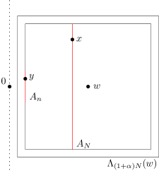
Figure 4: An illustration of the application of Proposition 3.2 in the proof of Lemma 3.5. We wish to argue that $G_{\beta}^{\mathbb{H}}(0,y)$ and $G_{\beta}^{\mathbb{H}}(0,x)$ are of the same order. The red segments represent the sets $A_{n}$ and $A_{N}$. The boxes are centered at $w=\tfrac{7N}{6}\mathbf{e}_{1}$. The parameter $\alpha$ is chosen so that $\Lambda_{(1+\alpha)N}(w)\subset\{z\in\mathbb{H},\>z_{1}\geq n/2\}$, i.e. $\alpha=\tfrac{1}{12}$.

We now turn to the full-plane lower bound below scale $5L_{\beta}(\varepsilon)$.

Lemma 3.6.

Fix $d>4$. There exist $c,\varepsilon_{0},\lambda_{0}>0$ such that for every $\lambda<\lambda_{0}$, every $\varepsilon<\varepsilon_{0}$, every $\tfrac{1}{2d}\leq\beta\leq\beta_{c}$, and every $|x|\leq 5L_{\beta}(\varepsilon)$,

$$G_{\beta}(0,x)\geq\frac{c}{|x|^{d-2}}.$$ (3.32)

Proof.

Let $\lambda_{0},\varepsilon_{0}$ be given by Lemma 3.5. We will choose $\lambda_{0}$ even smaller below. Let $\lambda<\lambda_{0}$ and $\varepsilon<\varepsilon_{0}$. By symmetry, we may consider $x\in A_{n}$, where $n=|x|$. Lemma 1.5 applied to $S=\mathbb{H}_{k}$ and $\Lambda=\mathbb{H}_{k+1}$ gives that

$$G_{\beta}(0,x)=G_{\beta}^{\mathbb{H}}(0,x)+\sum_{k\geq 0}\Big{(}G_{\beta}^{\mathbb{H}_{k+1}}(0,x)-G_{\beta}^{\mathbb{H}_{k}}(0,x)\Big{)}\\ \geq\sum_{k\geq 0}\sum_{\begin{subarray}{c}y\in\mathbb{H}_{k},\\ z\notin\mathbb{H}_{k},\>y\sim z\end{subarray}}G_{\beta}^{\mathbb{H}_{k}}(0,y)\beta G_{\beta}^{\mathbb{H}_{k+1}}(z,x)-\lambda\sum_{k\geq 0}\sum_{u\in\mathbb{H}_{k}}E_{\beta}^{\mathbb{H}_{k},\mathbb{H}_{k+1}}(u)G_{\beta}^{\mathbb{H}_{k+1}}(u,x).$$ (3.33)

Looking at the first sum, we see that

$$\sum_{k\geq 0}\sum_{\begin{subarray}{c}y\in\mathbb{H}_{k},\\ z\notin\mathbb{H}_{k},\>y\sim z\end{subarray}}G_{\beta}^{\mathbb{H}_{k}}(0,y)\beta G_{\beta}^{\mathbb{H}_{k+1}}(z,x) \geq\sum_{k=0}^{n\wedge(L_{\beta}(\varepsilon)-1)}\frac{1}{2d}\varphi_{\beta}(\Lambda_{k})\min\{G_{\beta}^{\mathbb{H}_{k+1}}(z,x):-z_{1}=|z|=k+1\}$$

$$\geq\sum_{k=0}^{n\wedge(L_{\beta}(\varepsilon)-1)}\frac{1}{2d}(1-\varepsilon)\frac{c}{(n+k)^{d-1}}$$

$$\geq\frac{c_{1}}{n^{d-2}},$$

where $c_{1}=c_{1}(d)>0$, and where we restricted our attention to special positions of $y$ and used both the bound $\varphi_{\beta}(\Lambda_{k})\geq 1-\varepsilon$ provided by $k\leq n\wedge(L_{\beta}(\varepsilon)-1)$ and the lower bound from Lemma 3.5 (note that $n+n\wedge L_{\beta}(\varepsilon)\leq 6L_{\beta}(\varepsilon)$ for $n\leq 5L_{\beta}(\varepsilon)$).

Turning to the “error” term in (3.33), we take the position of $u$ into account and use the upper bound (1.8) to get

$$\sum_{k\geq 0}\sum_{p\geq 0}\sum_{u\in\partial\mathbb{H}_{k-p}}\sum_{\begin{subarray}{c}y\in\mathbb{H}_{k}\\ z\notin\mathbb{H}_{k}\\ y\sim z\end{subarray}} G_{\beta}^{\mathbb{H}_{k}}(0,u)G_{\beta}^{\mathbb{H}_{k}}(u,y)\beta G_{\beta}^{\mathbb{H}_{k+1}}(z,u)G_{\beta}^{\mathbb{H}_{k+1}}(u,x)$$

$$\leq\sum_{k\geq 0}\sum_{p\geq 0}\frac{C}{(p+1)^{d-1}}\cdot\varphi_{\beta}(\mathbb{H}_{p})\cdot\sum_{u\in\partial\mathbb{H}_{k-p}}G_{\beta}^{\mathbb{H}_{k}}(0,u)G_{\beta}^{\mathbb{H}_{k+1}}(u,x).$$ (3.34)

Using Proposition 2.9, we have that $\varphi_{\beta}(\mathbb{H}_{p})\leq 1+K\lambda$. We bound (3.34) differently according to the value of $p$.

First, use (1.7) to get

$$\sum_{p\geq(n+k)/2}\frac{C(1+K\lambda)}{(p+1)^{d-1}}\sum_{u\in\partial\mathbb{H}_{k-p}}G_{\beta}^{\mathbb{H}_{k}}(0,u)G_{\beta}^{\mathbb{H}_{k+1}}(u,x) \leq\frac{C_{1}}{(n+k)^{d-1}}\sum_{u\in\mathbb{Z}^{d}}G_{\beta}(0,u)G_{\beta}(u,x)$$ (3.35)

$$\leq\frac{C_{2}}{(n+k)^{d-1}},$$ (3.36)

where $C_{1},C_{2}>0$ only depend on $C$ and $d$.

Second, turning to the contribution coming from $p<\tfrac{n+k}{2}$, we write

$$\max_{u\in\partial\mathbb{H}_{k-p}}G_{\beta}^{\mathbb{H}_{k+1}}(u,x)\stackrel{{\scriptstyle\eqref{eq: half plane at distance $k$ from half space}}}{{\leq}}\frac{2^{d}C(p+2)}{(n+k)^{d-1}},\qquad\sum_{u\in\partial\mathbb{H}_{k-p}}G_{\beta}^{\mathbb{H}_{k}}(0,u)\stackrel{{\scriptstyle\eqref{eq: sum at distance k from halfplane}}}{{\leq}}\frac{4(p+1)}{\beta},$$ (3.37)

where we used that for $u\in\partial\mathbb{H}_{k-p}$, one has $|u_{1}-x_{1}|=n+k-p\geq\tfrac{n+k}{2}$. Hence,

$$\sum_{p<(n+k)/2}\frac{C(1+K\lambda)}{(p+1)^{d-1}}\sum_{u\in\partial\mathbb{H}_{k-p}}G_{\beta}^{\mathbb{H}_{k}}(0,u)G_{\beta}^{\mathbb{H}_{k+1}}(u,x) \leq C_{3}\sum_{p\leq\tfrac{n+k}{2}}\frac{1}{(p+1)^{d-3}}\frac{1}{(n+k)^{d-1}}$$ (3.38)

$$\leq\frac{C_{4}}{(n+k)^{d-1}},$$ (3.39)

where $C_{3},C_{4}>0$ only depend on $C$ and $d$. Combining (3.36) and (3.39) gives that

$$\sum_{k\geq 0}\sum_{p\geq 0}\sum_{u\in\partial\mathbb{H}_{k-p}}\sum_{\begin{subarray}{c}y\in\mathbb{H}_{k}\\ z\notin\mathbb{H}_{k}\\ y\sim z\end{subarray}}G_{\beta}^{\mathbb{H}_{k}}(0,u)G_{\beta}^{\mathbb{H}_{k}}(u,y)\beta G_{\beta}^{\mathbb{H}_{k+1}}(z,u)G_{\beta}^{\mathbb{H}_{k+1}}(u,x) \leq\sum_{k\geq 0}\frac{C_{5}}{(n+k)^{d-1}}$$

$$\leq\frac{C_{6}}{n^{d-2}},$$ (3.40)

where $C_{5},C_{6}$ only depend on $C$ and $d$. The proof follows by choosing $\lambda_{0}$ small enough so that $\lambda_{0}C_{6}<c_{1}/2$, and setting $c=c_{1}/2$. ∎

We are now in a position to prove Theorem 1.2.

Proof of Theorem 1.2.

Let $\lambda_{0},\varepsilon_{0}>0$ be such that the previous two lemmata apply. We will (potentiallly) choose them even smaller below. Let $\lambda<\lambda_{0}$ and $\varepsilon<\varepsilon_{0}$.

Set $L^{\prime}_{\beta}:=L_{\beta}(\varepsilon)$. If $\beta=\beta_{c}$ then $L_{\beta}=L_{\beta}^{\prime}=\infty$ and the Lemmata 3.5 and 3.6 are sufficient to conclude. We therefore assume $\beta<\beta_{c}$. By Lemma 3.1 it suffices to prove the lower bounds with $L^{\prime}_{\beta}$ instead of $L_{\beta}$ in the exponential.

We already have the corresponding lower bounds for $|x|\leq 5L^{\prime}_{\beta}$. Let us turn to the general case. We focus on the full-space estimate but the half-space follows from a similar proof. Let $c>0$ be given by Lemma 3.6. Introduce, for $k\geq 0$,

$$m_{k} :=\min\{G_{\beta}(0,x):x\in\Lambda_{(k+1)L_{\beta}^{\prime}-1}\},$$ (3.41)

and $S_{k}:=\{x\in\mathbb{Z}^{d}:kL^{\prime}_{\beta}\leq|x|<(k+1)L^{\prime}_{\beta}\}$. We prove by induction for $k\geq 5$ that for some $c_{1}>0$,

$$m_{k}\geq\frac{c}{(5L^{\prime}_{\beta})^{d-2}}c_{1}^{k-5}.$$ (3.42)

For $k=5$, it is simply (3.27). We now assume that $k\geq 6$. Applying Lemma 1.5 (twice) and Lemma 2.4, there exists $c_{0}=c_{0}(d)>0$ such that for every $x\in S_{k}$,

$$G_{\beta}(0,x)\geq 2c_{0}m_{k-1}-2K\lambda M_{2}(x)$$ (3.46)

where for $\ell\geq 1$,

$$M_{\ell}(x) :=\max\{G_{\beta}(0,y):y\in\Lambda_{\ell L^{\prime}_{\beta}}(x)\}.$$ (3.47)

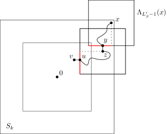
Figure 5: An illustration of the proof of (3.46). The situation depicted here is somehow the least favorable. The sets $H_{1}$ and $H_{2}$ are the red bold lines. With the two successive applications of Lemma 1.5, we “drive” the point $x$ towards the box $\Lambda_{kL_{\beta}^{\prime}-1}$. This provides a recurrence relation between $m_{k}$ and $m_{k-1}$.

If $x\in S_{k}$ is such that $2K\lambda M_{2}(x)\leq G_{\beta}(0,x)$, then (3.46) gives

$$G_{\beta}(0,x)\geq c_{0}m_{k-1}.$$ (3.48)

Moreover, when $x\in\Lambda_{kL_{\beta}^{\prime}-1}$,

$$G_{\beta}(0,x)\geq m_{k-1}\geq c_{0}m_{k-1}.$$ (3.49)

As a consequence, we find $m_{k}\geq c_{0}m_{k-1}$ and therefore the induction hypothesis (with $c_{1}=c_{0}$), except if there is $x\in S_{k}$ such that $2K\lambda M_{2}(x)>G_{\beta}(0,x)$. We show below that this is in fact impossible by proceeding by contradiction.

Let $\eta<\min\{1/(4C_{\rm RW}),c/(4C5^{d-2})\}$ and $\lambda_{0}<\eta/K$. Also, (potentially) decrease $\varepsilon_{0}$ so that Proposition 3.2 holds true for this $\eta$ and for $\alpha=1$.

For $\ell$ such that $0\notin\Lambda_{(\ell+4)L^{\prime}_{\beta}}(x)$, Proposition 3.2 applied to all boxes of size $2L^{\prime}_{\beta}$ centered on sites in $\Lambda_{\ell L_{\beta}^{\prime}}(x)$ gives

$$M_{\ell+2}(x)\leq C_{\rm RW}M_{\ell}(x)+\eta M_{\ell+4}(x).$$ (3.50)

Yet, the choices of $\eta$ and $\lambda_{0}$, as well as the assumption that

$$M_{0}(x)=G_{\beta}(0,x)<2K\lambda M_{2}(x)$$ (3.51)

imply recursively that $M_{\ell}(x)\leq 2\eta M_{\ell+2}(x)$ as long as $0\notin\Lambda_{(\ell+2)L^{\prime}_{\beta}}(x)$. In particular, if $L:=\lfloor|x|/L^{\prime}_{\beta}\rfloor-3$, we obtain that

$$\frac{c}{(5L^{\prime}_{\beta})^{d-2}}\stackrel{{\scriptstyle\eqref{eq:lb full below 5L}}}{{\leq}}m_{5}\leq M_{L}(x)\leq 2\eta M_{L+2}(x)\stackrel{{\scriptstyle\eqref{eq:upper bound below L}}}{{\leq}}2\eta\frac{2C}{(L^{\prime}_{\beta})^{d-2}}.$$ (3.52)

The choice of $\eta$ leads to a contradiction, therefore concluding the proof. ∎

Appendix: proof of Lemma 1.5

Write $\gamma$ as the concatenation $\gamma_{1}\circ(yz)\circ\gamma_{2}$, where $(yz)$ is the first edge exiting $S$ (with the convention that $y\in S$ and $z\notin S$). The structure of the weights implies that

$$\rho(\gamma_{1})\rho(\gamma_{2})-\lambda\rho(\gamma_{1})\rho(\gamma_{2})\sum_{\begin{subarray}{c}0\leq i\leq|\gamma_{1}|\\ 1\leq j\leq|\gamma_{2}|\end{subarray}}\mathds{1}_{\gamma_{1}(i)=\gamma_{2}(j)}\leq\rho(\gamma_{1}\circ(yz)\circ\gamma_{2})\leq\rho(\gamma_{1})\rho(\gamma_{2}),$$ (A.1)

where we used that

$$1-\lambda\sum_{\begin{subarray}{c}0\leq i\leq|\gamma_{1}|\\ 1\leq j\leq|\gamma_{2}|\end{subarray}}\mathds{1}_{\gamma_{1}(i)=\gamma_{2}(j)}\leq\prod_{\begin{subarray}{c}0\leq i\leq|\gamma_{1}|\\ 1\leq j\leq|\gamma_{2}|\end{subarray}}(1-\lambda\mathds{1}_{\gamma_{1}(i)=\gamma_{2}(j)}).$$ (A.2)

After observing that $\gamma_{1}\subset S$, resumming the right-hand side of (A.1) gives the upper bound of (1.19).

For the lower bound, note that conditioning on the common value $u$ of $\gamma_{1}(i)$ and $\gamma_{2}(j)$, the “error” is controlled by

$$\lambda\sum_{u\in S}\sum_{\begin{subarray}{c}y\in S\\ z\notin S\\ y\sim z\end{subarray}}\sum_{n,m\geq 0}\beta^{n+m+1}\sum_{\begin{subarray}{c}0\leq i\leq n\\ 1\leq j\leq m\end{subarray}}\sum_{\begin{subarray}{c}\gamma_{1}:0\rightarrow y\subset S\\ \gamma_{2}:z\rightarrow x\subset\Lambda\end{subarray}}\rho(\gamma_{1})\rho(\gamma_{2})\mathds{1}_{\gamma_{1}(i)=u,\>|\gamma_{1}|=n}\mathds{1}_{\gamma_{2}(j)=u,\>|\gamma_{2}|=m}.$$ (A.3)

We further split $\gamma_{1}$ into $\gamma_{1}^{\prime}:0\rightarrow u$ and $\gamma_{1}^{\prime\prime}:u\rightarrow t$ and use that $\rho(\gamma_{1})\leq\rho(\gamma_{1}^{\prime})\rho(\gamma_{1}^{\prime\prime})$, and do the same for $\gamma_{2}$. Note that by definition, $|\gamma_{1}^{\prime}|=i$ and $|\gamma_{1}^{\prime\prime}|=n-i$. Similarly, $|\gamma_{2}^{\prime}|=j$ and $|\gamma_{2}^{\prime\prime}|=m-j$. The Cauchy product implies that

$$\sum_{n\geq 0}\sum_{i=0}^{n}\beta^{n}\sum_{\begin{subarray}{c}\gamma_{1}^{\prime}:0\rightarrow u\subset S\\ \gamma_{1}^{\prime\prime}:u\rightarrow y\subset S\end{subarray}}\rho(\gamma_{1}^{\prime})\mathds{1}_{|\gamma_{1}^{\prime}|=i}\rho(\gamma_{1}^{\prime\prime})\mathds{1}_{|\gamma_{1}^{\prime\prime}|=n-i}=G^{S}_{\beta}(0,u)G^{S}_{\beta}(u,y).$$ (A.4)

Similarly,

$$\sum_{m\geq 0}\sum_{j=1}^{m}\beta^{m}\sum_{\begin{subarray}{c}\gamma_{2}^{\prime}:z\rightarrow u\subset\Lambda\\ \gamma_{2}^{\prime\prime}:u\rightarrow x\subset\Lambda\end{subarray}}\rho(\gamma_{2}^{\prime})\mathds{1}_{|\gamma_{1}^{\prime}|=j}\rho(\gamma_{2}^{\prime\prime})\mathds{1}_{|\gamma_{2}^{\prime\prime}|=m-j}\leq G^{B}_{\beta}(z,u)G^{B}_{\beta}(u,x).$$ (A.5)

This yields

$$G^{\Lambda}_{\beta}(0,x)-\sum_{\begin{subarray}{c}y\in S\\ z\notin S\\ y\sim z\end{subarray}}G_{\beta}^{S}(0,y)\beta G_{\beta}^{\Lambda}(z,x)\leq\lambda\sum_{u\in S}\sum_{\begin{subarray}{c}y\in S\\ z\notin S\\ y\sim z\end{subarray}}G^{S}_{\beta}(0,u)G^{S}_{\beta}(u,y)\beta G^{\Lambda}_{\beta}(z,u)G^{\Lambda}_{\beta}(u,x),$$ (A.6)

and concludes the proof.

References

- [BBS14] Roland Bauerschmidt, David C. Brydges, and Gordon Slade. Scaling limits and critical behaviour of the -dimensional -component spin model. Journal of Statistical Physics, 157:692–742, 2014.
- [BBS15a] Roland Bauerschmidt, David C. Brydges, and Gordon Slade. Critical two-point function of the 4-dimensional weakly self-avoiding walk. Communications in Mathematical Physics, 338:169–193, 2015.
- [BBS15b] Roland Bauerschmidt, David C. Brydges, and Gordon Slade. Logarithmic correction for the susceptibility of the 4-dimensional weakly self-avoiding walk: a renormalisation group analysis. Communications in Mathematical Physics, 337:817–877, 2015.
- [BBS19] Roland Bauerschmidt, David C. Brydges, and Gordon Slade. Introduction to a Renormalisation Group Method, volume 2242. Springer Nature, 2019.
- [BDCGS12] Roland Bauerschmidt, Hugo Duminil-Copin, Jesse Goodman, and Gordon Slade. Lectures on self-avoiding walks. Probability and Statistical Physics in Two and More Dimensions (D. Ellwood, CM Newman, V. Sidoravicius, and W. Werner, eds.), Clay Mathematics Institute Proceedings, 15:395–476, 2012.
- [BFF84] Anton Bovier, Giovanni Felder, and Jürg Fröhlich. On the critical properties of the Edwards and the self-avoiding walk model of polymer chains. Nuclear Physics B, 230(1):119–147, 1984.
- [BHH21] David Brydges, Tyler Helmuth, and Mark Holmes. The continuous-time lace expansion. Communications on Pure and Applied Mathematics, 74(11):2251–2309, 2021.
- [BHK18] Erwin Bolthausen, Remco W. van der Hofstad, and Gady Kozma. Lace expansion for dummies. Annales de l’Institut Henri Poincaré - Probabilités et Statistiques, 54(1):141–153, 2018.
- [BS85] David Brydges and Thomas Spencer. Self-avoiding walk in 5 or more dimensions. Communications in Mathematical Physics, 97(1):125–148, 1985.
- [DCP24a] Hugo Duminil-Copin and Romain Panis. An alternative approach for the mean-field behaviour of spread-out Bernoulli percolation in dimensions . preprint, 2024.
- [DCP24b] Hugo Duminil-Copin and Romain Panis. New lower bounds for the (near) critical Ising and models’ two-point functions. arXiv preprint arXiv:2404.05700, 2024.
- [DCT16] Hugo Duminil-Copin and Vincent Tassion. A new proof of the sharpness of the phase transition for Bernoulli percolation and the Ising model. Communications in Mathematical Physics, 343:725–745, 2016.
- [FvdH17] Robert Fitzner and Remco W. van der Hofstad. Mean-field behavior for nearest-neighbor percolation in . Electronic Journal of Probability, 22:43, 2017.
- [Har08] Takashi Hara. Decay of correlations in nearest-neighbor self-avoiding walk, percolation, lattice trees and animals. The Annals of Probability, 36(2):530–593, 2008.
- [HS90a] Takashi Hara and Gordon Slade. Mean-field critical behaviour for percolation in high dimensions. Communications in Mathematical Physics, 128(2):333–391, 1990.
- [HS90b] Takashi Hara and Gordon Slade. On the upper critical dimension of lattice trees and lattice animals. Journal of statistical physics, 59:1469–1510, 1990.
- [HS92] Takashi Hara and Gordon Slade. Self-avoiding walk in five or more dimensions I. The critical behaviour. Communications in Mathematical Physics, 147(1):101–136, 1992.
- [HvdHS03] Takashi Hara, Remco W. van der Hofstad, and Gordon Slade. Critical two-point functions and the lace expansion for spread-out high-dimensional percolation and related models. The Annals of Probability, 31(1):349–408, 2003.
- [Liu23] Yucheng Liu. A general approach to massive upper bound for two-point function with application to self-avoiding walk torus plateau. arXiv preprint arXiv:2310.17321, 2023.
- [LL10] Gregory F. Lawler and Vlada Limic. Random walk: a modern introduction, volume 123. Cambridge University Press, 2010.
- [MS93] Neal Madras and Gordon Slade. The Self-Avoiding Walk. Birkhäuser, Boston, (1993).
- [Pan23] Romain Panis. Triviality of the scaling limits of critical Ising and models with effective dimension at least four. arXiv preprint arXiv:2309.05797, 2023.
- [Sak07] Akira Sakai. Lace expansion for the Ising model. Communications in Mathematical Physics, 272(2):283–344, 2007.
- [Sak15] Akira Sakai. Application of the lace expansion to the model. Communications in Mathematical Physics, 336:619–648, 2015.
- [Sak22] Akira Sakai. Correct bounds on the Ising lace-expansion coefficients. Communications in Mathematical Physics, 392(3):783–823, 2022.
- [Sim80] Barry Simon. Correlation inequalities and the decay of correlations in ferromagnets. Communications in Mathematical Physics, 77(2):111–126, 1980.
- [Sla87] Gordon Slade. The diffusion of self-avoiding random walk in high dimensions. Communications in Mathematical Physics, 110:661–683, 1987.
- [Sla06] Gordon Slade. The Lace Expansion and Its Applications: Ecole D’Eté de Probabilités de Saint-Flour XXXIV-2004. Springer, 2006.
- [Sla22] Gordon Slade. A simple convergence proof for the lace expansion. In Annales de l’Institut Henri Poincaré (B) Probabilites et Statistiques, volume 58, pages 26–33, 2022.
- [Sla23] Gordon Slade. The near-critical two-point function and the torus plateau for weakly self-avoiding walk in high dimensions. Mathematical Physics, Analysis and Geometry, 26(1):6, 2023.