Unlearnable 3D Point Clouds: Class-wise Transformation Is All You Need
Abstract
Traditional unlearnable strategies have been proposed to prevent unauthorized users from training on the 2D image data. With more 3D point cloud data containing sensitivity information, unauthorized usage of this new type data has also become a serious concern. To address this, we propose the first integral unlearnable framework for 3D point clouds including two processes: (i) we propose an unlearnable data protection scheme, involving a class-wise setting established by a category-adaptive allocation strategy and multi-transformations assigned to samples; (ii) we propose a data restoration scheme that utilizes class-wise inverse matrix transformation, thus enabling authorized-only training for unlearnable data. This restoration process is a practical issue overlooked in most existing unlearnable literature, i.e., even authorized users struggle to gain knowledge from 3D unlearnable data. Both theoretical and empirical results (including 6 datasets, 16 models, and 2 tasks) demonstrate the effectiveness of our proposed unlearnable framework. Our code is available at https://github.com/CGCL-codes/UnlearnablePC
1 Introduction
Recently, 3D point cloud deep learning has been making remarkable strides in various domains, e.g., self-driving [5] and virtual reality [1, 44]. Specifically, numerous 3D sensors scan the surrounding environment and synthesize massive 3D point cloud data containing sensitive information such as pedestrian and vehicles [30] to the cloud server for deep learning analysis [10, 21]. However, the raw point cloud data can be exploited for point cloud unauthorized deep learning if a data breach occurs, posing a significant privacy threat. Fortunately, the privacy protection approaches for preventing unauthorized training have been extensively studied in the 2D image domain [8, 17, 26, 27, 37, 40]. They apply elaborate perturbations on images such that trained networks over them exhibit extremely low generalization, thus failing to learn knowledge from the protected data, known as "making data unlearnable". Nonetheless, the stark disparity between 2D images and 3D point clouds poses significant challenges for drawing lessons from existing 2D solutions.
Specifically, migrating 2D unlearnable schemes to 3D suffers from following challenges: (i) Incompatibility with 3D data. Numerous model-agnostic 2D image unlearnable schemes operate in the pixel space, such as convolutional operations [37, 40], making them fail to be directly transferred to the 3D point space. (ii) Poor visual quality. Migrating model-dependent 2D unlearnable methods [4, 8, 17, 26] to 3D point clouds requires perturbing substantial points, leading to irregular three-dimensional shifts which may significantly degrade visual quality. Hence, these challenges spur us to start directly from the characteristics of point clouds for proposing 3D unlearnable solutions.
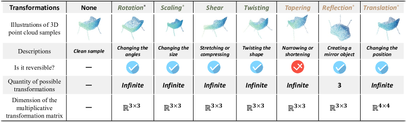
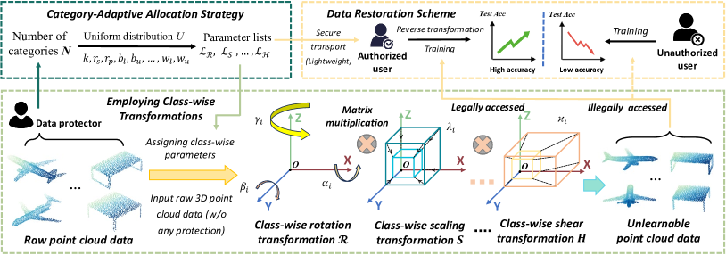
Recent works observe that 3D transformations can alter test-time results of models [6, 15, 42]. To explore this, we conduct an in-depth investigation into the properties of seven 3D transformations as shown in Fig. 1 and reveal the mechanisms by which transformations employed in a certain pattern serve as unlearnable schemes (Sec. 3.2). In light of this, we propose the first unlearnable approach in 3D point clouds via multi class-wise transformation (UMT), transforming samples to various forms for privacy protection. Concretely, we newly propose a category-adaptive allocation strategy by leveraging uniform distribution sampling and category constraints to establish a class-wise setting, thereby multiplying multi-transformations to samples based on categories. To theoretically analyze UMT, we define a binary classification setup similar to that used in [18, 31, 37]. Meanwhile, we employ a Gaussian Mixture Model (GMM) [36] to model the clean training set and use the Bayesian optimal decision boundary to model the point cloud classifier. Theoretically, we prove that there exists a UMT training set follows a GMM distribution and the classification accuracy of UMT dataset is lower than that of the clean dataset in a Bayesian classifier.
Moreover, an incompatible issue in existing unlearnable works [8, 17, 26, 27, 37, 41] was identified [52], i.e., these approaches prevent unauthorized learning to protected data, but they also impede authorized users from effectively learning from unlearnable data. To address this, we propose a data restoration scheme that applies class-wise inverse transformations, determined by a lightweight message received from the protector. Our proposed unlearnable framework including UMT approach and data restoration scheme is depicted in Fig. 3.
Extensive experiments on 6 benchmark datasets (including synthetic and real-world datasets) using 16 point cloud models across CNN, MLP, Graph-based Network, and Transformer on two tasks (classification and semantic segmentation), verified the effectiveness of our proposed unlearnable scheme. We summarize our main contributions as follows:
-
•
The First Integral 3D Unlearnable Framework. To the best of our knowledge, we propose the first integral unlearnable 3D point cloud framework, utilizing class-wise multi-transformation as its unlearnable mechanism (effectively safeguarding point cloud data against unauthorized exploitation) and proposing a novel data restoration approach that leverages class-wise reversible 3D transformation matrices (addressing an incompatible issue in most existing unlearnable works, where even authorized users cannot effectively learn knowledge from unlearnable data).
-
•
Theoretical Analysis. We theoretically indicate the existence of an unlearnable situation that the classification accuracy of the UMT dataset is lower than that of the clean dataset under the decision boundary of the Bayes classifier in Gaussian Mixture Model.
-
•
Experimental Evaluation. Extensive experiments on 3 synthetic datasets and 3 real-world datasets using 16 widely used point cloud model architectures on classification and semantic segmentation tasks verify the superiority of our proposed schemes.
2 Preliminaries
Notation. Considering the raw point cloud data sampled from a clean distribution for training a point cloud network, the user’s goal is to obtain a model by minimizing the loss function (e.g., cross-entropy loss) . Let be a 3D transformation matrix that does not seriously damage the visual quality of point clouds. Note that , , and represents the number of points. In theoretical analysis, following [18, 31], we simplify a training dataset to a Gaussian Mixture Model (GMM) [36] , where denotes the class labels, denotes the mean value, and denotes the identity matrix. Thus the Bayes optimal decision boundary for classifying is defined by . The accuracy of the decision boundary on is equal to , where denotes the Cumulative Distribution Function (CDF) of the standard normal distribution.
Data protector . aims to protect the knowledge from the clean training set (with size of ) by compromising the unauthorized models who train on the unlearnable point cloud data , resulting in extremely poor generalization on the clean test distribution . This objective can be formalized as:
| (1) |
where assumes that training samples are all transformed into unlearnable ones while maintaining normal visual effects, in line with previous unlearnable works [17, 26, 37, 40]. By the way, solving Eq. 1 directly is infeasible for neural networks because it necessitates unrolling the entire training procedure within the inner objective and performing backpropagation through it to execute a single step of gradient descent on the outer objective [7].
Authorized user . aims to apply another transformation on the unlearnable sample, making the protected data learnable. This is formally defined as:
| (2) |
where assumes that, without access to any clean training samples, can be constructed by utilizing a lightweight message received from data protectors.
3 Our Proposed Unlearnable Schemes
3.1 Key Intuition
Several recent works [6, 11, 42] reveal employing 3D transformations can mislead the model’s classification results. Such a phenomenon implies that there might be some defects in point cloud classifiers when processing transformed samples, leading us to infer that 3D transformations are probable candidates for data protection against unauthorized training. If the transformed point cloud data are used to train unauthorized DNNs, only simple linear features inherent in 3D transformations (at which transformations may act as shortcuts [12]) are captured by the DNNs, successfully protecting point cloud data privacy.
3.2 Exploring the Mechanism
We summarize existing 3D transformations in Fig. 1 and formally define them in Appendix A. To seek clarity on the application and selection of transformations, we explore three aspects: (i) execution mechanism, (ii) exclusion mechanism, and (iii) working mechanism as follows.
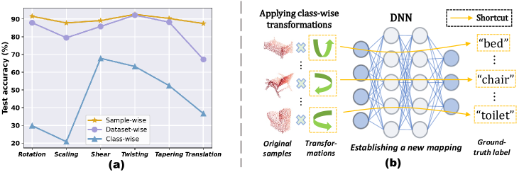
(i) Which execution mechanism successfully satisfy Eq. 1? The extensively employed execution patterns in 2D unlearnable approaches are sample-wise [8, 17] and class-wise [17, 37] settings. We further complement the dataset-wise setting (using universal transformation) and implement the above execution mechanisms for training a PointNet classifier [33] on the transformed ModelNet10 [48], obtaining test accuracy results in Fig. 2 (a). We discover that model achieves considerably low test accuracy under the class-wise setting, satisfying Eq. 1. Sample-wise and dataset-wise settings do not obviously compromise model performance, which cannot serve as promising unlearnable routes. Moreover, we note that sample-wise transformation is often considered as a data augmentation scheme to improve generalization, which contradicts our aim of using class-wise transformation to lower model generalization.
(ii) Which transformations need to be excluded? Not all transformations are suitable candidates. We exclude three transformations, tapering, reflection, and translation. (1) The tapering matrix may cause point cloud samples to become a planar projection when defined in Eq. 18 equals to -1, rendering the tapered samples meaningless; (2) The reflection matrix has only three distinct transformation matrices, rendering it incapable of assigning class-wise transformations when the number of categories exceeds three; (3) The translation transformation is a straightforward and simple additive transformation that is too easily defeated by point cloud data pre-processing approaches.
(iii) Why does class-wise transformation work? We conduct experiments using class-wise transformations (see Tab. 6), indicating that the model training on the class-wise transformed training set achieves a relatively high accuracy on the class-wise transformed test set (using the same transformation process as the training set). Besides, if we permute the class-wise transformation for the test set, we obtain a significant low accuracy on the test set. Therefore, we conclude that the reason why class-wise transformation works is that the model learns the mapping between class-wise transformations and corresponding category labels as shown in Fig. 2 (b), which results in the model being unable to predict the corresponding labels on a clean test set lacking transformations. This analytical process yields conclusions that are in agreement with prior research [37, 42].
3.3 Our Design for UMT
3.3.1 Category-Adaptive Allocation Strategy
We assign transformation parameters based on categories to realize class-wise setting. For rotation transformation , we refer to and as slight angles imposed on the and axes, as the primary angle for axis. We generate random angles for times in three directions:
| (3) |
where denotes uniform distribution, denotes the number of categories, is a small range that controls and , while is a large range that controls . is computed in such a way to ensure that the number of combinations of three angles is greater than or equal to . Concretely, in the rotation operation, each of the three directions has distinct angles, which means that the final rotation matrix has possible combinations. To satisfy the class-wise setup, must be at least , requiring to be no less than . Finally, we randomly select combinations of angles for the allocation. The scaling transformation resizes the position of each point in the 3D point cloud sample by a certain scaling factor , which is sampled times from a uniform distribution :
| (4) |
where and represent the lower bound and upper bound of the scaling factor, respectively. For shear defined in Eq. 13, twisting defined in Eq. 16, the process of generating parameters within ranges and is consistent to scaling. The range of these parameters ensures the visual effect of the sample.
Property 1. Since rotation matrices , , and around three directions are all orthogonal matrices, is also an orthogonal matrix, which can be defined as:
| (5) |
where we can determine the orthogonality by matrix multiplication through the definitions of Eq. 11. Since and , so is also an orthogonal matrix.
Property 2. All four transformation matrices we employ, , , , and , and the multiplicative combinations of any these matrices are all invertible matrices, which can be formally defined as:
| (6) |
where the inverse matrices of , , , and are given in Appendix A. This property allows the authorized users to normally train on the protected data due to that multiplying a matrix by its inverse results in the identity matrix, leading us to propose a data restoration scheme in Sec. 3.4.
3.3.2 Employing Class-wise Transformations
Assuming the point cloud training set is defined as , where represent the number of samples in the 1st, 2nd, …, -th category, respectively. We formally define the spectrum of transformations as to indicate the number of transformations involved. Thus the ultimate unlearnable transformation matrix is defined as:
| (7) |
Once we employ the proposed category-adaptive allocation strategy to , the unlearnable point cloud dataset is constructed as:
| (8) |
Our proposed UMT scheme is described in Algorithm 1. We enumerate possible transformations in Eq. 7 to obtain the unlearnability in Tab. 7 and select one type of class-wise transformation for each for more comprehensive experiments in Tab. 1. To facilitate the theoretical study of UMT111In the subsequent theoretical descriptions, UMT refers to UMT with =2 using transformation matrix ., we opt for as the transformation matrix , which achieves the best unlearnable effect as suggested in Tabs. 1 and 7. Thus, in the GMM scenario, the class-wise transformation matrix is defined as , where is the scaling factor.
Lemma 3. The unlearnable dataset generated using UMT on can also be represented using a GMM, i.e., .
Proof: See Sec. D.1. Lemma 3 demonstrates that the unlearnable dataset can also be represented as a GMM, which is derived from Property 1.
Lemma 4. The Bayes optimal decision boundary for classifying is given by , where , , and .
Proof: See Sec. D.2. Lemma 4 reveals that the Bayesian decision boundary for classifying is a quadratic surface based on the GMM expression of .
Lemma 5. Let , , where , and denote 2-norm of vectors. For any and , we employ Chernoff bound to have:
Proof: See Sec. D.3. Lemma 5 enables us to establish an upper bound on the accuracy of the unlearnable decision boundary applied to the clean dataset , denoted as , as presented in Theorem 6 below.
Theorem 6. For any constant and satisfying and , the accuracy of the unlearnable decision boundary on can be upper-bounded as:
Furthermore, if and , we have . Moreover, for any , matrix such that , where is the Bayes optimal decision boundary for classifying .
Proof: See Sec. D.4. The unlearnable effect takes place when . To achieve this, we elaborately choose , which is formalized as . Therefore, Theorem 6 theoretically explains why UMT is effective in generating unlearnable point cloud data.
3.4 Data Restoration Scheme
To ensure that authorized users can achieve better generalization after training on unlearnable data, i.e., satisfying Eq. 2, we exploit the inverse properties of 3D transformations, presented in Property 2, to calculate the inverse matrix of as:
| (9) |
In particular, we note that , . Afterwards, the authorized user receives a lightweight message containing class-wise parameters from the data protector through a secure channel, thereby assigning to the inverse transformation matrix in Eq. 9 for multiplying the unlearnable samples. Our proposed integral unlearnable process is illustrated in Fig. 3.
4 Experiments
4.1 Experimental Details
Datasets and Models. Three synthetic 3D point cloud datasets, ModelNet40 [48], ModelNet10 [48], ShapeNetPart [3] and three real-world datasets including autonomous driving dataset KITTI [30] and indoor datasets ScanObjectNN [39], S3DIS [2] are used. We choose 16 widely used 3D point cloud models PointNet [33], PointNet++ [34], DGCNN [43], PointCNN [23], PCT [14], PointConv [46], CurveNet [49], SimpleView [13], 3DGCN [24], LGR-Net [57], RIConv [55], RIConv++ [56], PointMLP [29], PointNN [54], PointTransformerV3 [47], and SegNN [60] for evaluation of classification and semantic segmentation tasks.
| Datasets | Schemes | PointNet | PointNet++ | DGCNN | PointCNN | PCT | PointConv | CurveNet | SimpleView | RIConv++ | 3DGCN | PointNN | PointMLP | AVG |
|---|---|---|---|---|---|---|---|---|---|---|---|---|---|---|
| ModelNet10 | Clean | 89.85±0.54 | 92.11±1.57 | 91.81±0.84 | 87.99±1.58 | 90.18±2.23 | 91.26±1.12 | 91.88±1.51 | 89.52±0.41 | 87.90±1.64 | 88.51±5.39 | 83.22±0.73 | 91.07±0.19 | 89.61±0.42 |
| UMT(k=1) | 40.64±10.69 | 28.73±2.00 | 27.41±6.71 | 32.82±2.70 | 31.58±4.27 | 33.64±6.63 | 39.78±6.80 | 45.31±11.85 | 86.72±1.46 | 28.01±8.72 | 34.47±0.29 | 32.85±2.35 | 38.50±2.01 | |
| UMT(k=2) | 21.18±0.93 | 26.36±1.71 | 18.84±6.14 | 21.97±4.04 | 19.72±4.52 | 20.84±5.96 | 25.04±2.15 | 22.75±2.43 | 16.53±3.63 | 32.79±3.23 | 31.94±2.11 | 25.41±3.96 | 23.61±1.06 | |
| UMT(k=3) | 22.84±1.71 | 23.81±8.43 | 29.16±4.30 | 27.03±9.97 | 29.43±9.11 | 18.49±7.39 | 25.51±9.57 | 32.12±12.58 | 19.94±1.13 | 36.19±13.38 | 30.54±1.24 | 32.21±5.28 | 27.27±6.20 | |
| UMT(k=4) | 18.83±2.40 | 20.56±14.61 | 15.92±1.51 | 20.52±6.06 | 20.29±2.14 | 21.66±2.24 | 23.46±12.58 | 24.12±6.20 | 26.41±2.47 | 34.28±17.20 | 25.59±0.25 | 26.65±11.36 | 23.19±5.98 | |
| ModelNet40 | Clean | 86.18±0.07 | 90.55±0.73 | 89.51±0.86 | 81.89±5.35 | 87.11±1.39 | 88.90±0.89 | 87.82±0.23 | 85.25±0.31 | 84.59±1.07 | 86.81±1.69 | 74.81±0.16 | 87.31±0.91 | 85.89±0.40 |
| UMT(k=1) | 28.62±1.80 | 20.69±0.87 | 28.60±1.65 | 21.92±1.86 | 29.06±0.38 | 24.99±2.63 | 33.29±3.92 | 26.89±1.48 | 75.86±8.43 | 26.30±1.92 | 28.57±0.39 | 29.28±1.72 | 31.17±0.20 | |
| UMT(k=2) | 8.30±0.87 | 18.71±1.65 | 11.60±1.97 | 10.85±2.61 | 9.21±2.31 | 12.99±0.99 | 12.71±3.70 | 12.05±3.88 | 10.48±2.01 | 26.17±0.35 | 25.05±0.06 | 10.90±4.74 | 14.09±0.78 | |
| UMT(k=3) | 7.48±1.66 | 17.62±3.10 | 10.41±5.48 | 9.43±3.09 | 9.91±4.19 | 11.28±4.93 | 11.23±3.07 | 11.21±4.09 | 10.92±0.48 | 25.31±1.29 | 24.53±0.10 | 8.94±3.43 | 13.19±2.41 | |
| UMT(k=4) | 7.83±2.25 | 15.72±4.12 | 10.86±2.57 | 8.60±2.28 | 9.68±1.58 | 10.52±2.09 | 10.91±3.00 | 14.32±0.92 | 18.09±3.83 | 17.16±5.47 | 24.31±0.28 | 12.38±1.51 | 13.36±0.43 | |
| ShapeNetPart | Clean | 98.21±0.03 | 98.50±0.12 | 98.06±0.65 | 97.54±0.22 | 96.38±0.84 | 98.23±0.23 | 98.42±0.08 | 98.26±0.21 | 96.70±0.64 | 96.18±1.90 | 94.66±0.11 | 98.39±0.12 | 97.46±0.22 |
| UMT(k=1) | 63.85±12.71 | 50.30±21.71 | 64.71±13.44 | 51.95±14.13 | 54.39±3.36 | 29.34±0.14 | 71.38±9.34 | 56.22±6.48 | 96.93±0.09 | 37.90±9.67 | 58.44±0.61 | 47.32±8.26 | 56.89±3.00 | |
| UMT(k=2) | 18.41±6.45 | 45.61±4.64 | 25.99±2.73 | 28.97±3.73 | 37.72±16.26 | 25.60±8.59 | 26.49±8.58 | 38.38±5.96 | 5.05±3.63 | 32.21±13.01 | 49.82±1.56 | 34.19±4.43 | 30.70±1.43 | |
| UMT(k=3) | 32.50±10.03 | 39.64±12.52 | 37.29±11.20 | 46.77±19.59 | 43.52±22.24 | 31.28±4.67 | 37.27±10.30 | 41.51±2.66 | 6.01±6.11 | 47.84±7.05 | 50.85±0.07 | 47.80±21.37 | 38.52±6.17 | |
| UMT(k=4) | 23.72±15.04 | 23.30±4.43 | 36.18±10.00 | 34.52±16.15 | 45.07±18.99 | 29.48±11.09 | 29.79±4.79 | 40.04±9.97 | 32.22±1.38 | 33.06±28.16 | 51.91±0.03 | 40.93±21.81 | 35.02±11.23 | |
| KITTI | Clean | 98.04±2.23 | 99.49±0.50 | 99.33±0.34 | 99.23±0.25 | 98.93±0.54 | 98.04±1.68 | 99.10±1.05 | 99.38±0.33 | 99.64±0.09 | 99.67±0.24 | 99.49±0.50 | 95.72±5.46 | 98.84±0.87 |
| UMT(k=1) | 36.23±30.18 | 62.90±20.51 | 38.93±33.08 | 57.80±13.99 | 58.26±21.66 | 39.99±6.82 | 33.33±10.75 | 56.71±30.96 | 98.53±1.19 | 68.34±10.46 | 70.34±0.98 | 47.20±20.79 | 55.71±5.54 | |
| UMT(k=2) | 31.24±7.11 | 51.07±20.29 | 27.90±10.33 | 49.69±11.52 | 51.47±17.36 | 25.95±11.38 | 20.55±4.93 | 51.77±8.53 | 99.80±0.09 | 70.42±27.97 | 47.31±10.58 | 39.90±10.00 | 47.26±5.95 | |
| UMT(k=3) | 19.13±6.93 | 53.73±12.44 | 31.26±21.68 | 56.08±17.90 | 54.45±11.77 | 42.54±21.46 | 27.38±19.20 | 32.62±11.76 | 98.48±1.61 | 69.51±8.27 | 70.14±1.30 | 58.44±6.61 | 51.15±4.79 | |
| UMT(k=4) | 26.84±16.26 | 61.79±6.65 | 29.89±15.72 | 54.27±11.99 | 64.21±10.76 | 57.29±12.05 | 37.70±11.60 | 54.63±13.07 | 99.34±0.23 | 72.33±3.47 | 70.49±0.76 | 56.25±12.33 | 57.09±5.97 | |
| ScanObjectNN | Clean | 65.20±1.49 | 77.38±2.60 | 72.66±2.56 | 66.96±6.42 | 50.75±15.16 | 75.42±2.06 | 70.92±1.06 | 51.93±2.89 | 66.34±1.21 | 73.84±2.75 | 58.17±0.30 | 73.32±1.39 | 66.91±0.72 |
| UMT(k=1) | 56.55±0.11 | 63.01±2.38 | 57.93±3.11 | 51.97±11.99 | 47.05±7.12 | 56.71±3.61 | 65.49±3.15 | 38.96±2.08 | 62.33±10.68 | 52.89±1.13 | 54.56±0.17 | 62.96±4.19 | 55.87±0.95 | |
| UMT(k=2) | 14.55±1.81 | 49.41±3.44 | 20.96±3.99 | 13.61±4.97 | 15.10±2.05 | 20.78±4.74 | 21.35±2.59 | 20.73±9.64 | 10.76±1.76 | 52.37±5.62 | 48.25±0.20 | 16.32±4.78 | 25.35±0.49 | |
| UMT(k=3) | 10.92±3.87 | 41.96±3.84 | 14.62±5.56 | 10.62±2.35 | 22.02±7.83 | 19.96±3.13 | 21.43±8.67 | 11.79±3.96 | 11.69±1.41 | 56.32±0.83 | 48.94±0.70 | 23.05±16.32 | 24.44±2.46 | |
| UMT(k=4) | 5.77±2.10 | 34.65±8.31 | 12.16±4.84 | 9.87±0.95 | 17.86±11.63 | 12.79±7.46 | 15.28±4.86 | 20.09±6.26 | 31.83±2.20 | 46.06±14.07 | 45.27±0.17 | 8.76±3.18 | 21.70±3.61 |
Experimental setup. The training process involves Adam optimizer [20], CosineAnnealingLR scheduler [28], initial learning rate of 0.001, weight decay of 0.0001. We empirically set , , , , , , , and to 15∘, 120∘, 0.6, 0.8, 0∘, 20∘, 0, and 0.4 respectively. The main results of different on unlearnability is shown in Tab. 1. Specifically, uses , uses , uses , and uses . More results for different combinations of class-wise transformations are provided in Tab. 7. The table values covered by gray denote the best unlearnable effect.
| Pre-process schemes | PointNet | PointNet++ | DGCNN | PointCNN | CurveNet | SimpleView | RIConv++ | 3DGCN | PointNN | PointMLP | AVG |
|---|---|---|---|---|---|---|---|---|---|---|---|
| Clean baseline | 86.10 | 91.13 | 89.02 | 75.73 | 87.76 | 85.49 | 85.82 | 84.89 | 75.00 | 87.66 | 84.86 |
| \hdashlineSOR | 9.93 | 19.17 | 9.36 | 10.45 | 11.57 | 14.81 | 6.66 | 25.08 | 25.04 | 15.22 | 14.73 |
| SRS | 9.24 | 22.20 | 10.25 | 7.78 | 12.66 | 14.04 | 11.32 | 24.72 | 26.01 | 12.18 | 15.04 |
| Random rotation | 10.94 | 26.74 | 11.59 | 10.21 | 12.13 | 6.86 | 12.09 | 55.64 | 29.74 | 20.37 | 19.63 |
| Random scaling | 22.33 | 22.45 | 30.15 | 20.22 | 25.61 | 23.25 | 73.62 | 27.48 | 26.50 | 24.39 | 29.60 |
| Random jitter | 9.64 | 21.72 | 10.05 | 7.74 | 9.98 | 16.68 | 13.27 | 23.74 | 26.90 | 9.09 | 14.88 |
| \hdashlineRandom rotation & scaling | 63.49 | 34.44 | 44.65 | 37.56 | 72.89 | 51.62 | 78.04 | 64.00 | 36.26 | 78.94 | 56.19 |
Evaluation Metrics. For classification, we report the (in %) derived from the classification accuracy on clean test set, which aligns with the metrics used in the 2D unlearnable schemes [17, 26, 37]. For semantic segmentation, we use and mean Intersection over Union (mIoU) as evaluation metrics (in %), where is the ratio of the number of points classified correctly to the total number of points in the point cloud, mIoU calculates the IoU for each class between the ground truth and the predicted segmentation [59], and then takes the average of these ratios. The lower these metrics are, the better the effect of the unlearnable scheme.
| Evaluation metrics | Eval accuracy (%) | mIoU (%) | ||||||
|---|---|---|---|---|---|---|---|---|
| Segmentation models | PointNet++ [34] | Point Transformer v3 [47] | SegNN [60] | AVG | PointNet++ [34] | Point Transformer v3 [47] | SegNN [60] | AVG |
| Clean baseline | 74.76 | 74.72 | 79.00 | 76.16 | 40.06 | 40.57 | 50.27 | 43.63 |
| UMT(k=2) | 15.89 | 25.61 | 66.41 | 35.97 | 7.45 | 18.32 | 46.30 | 24.02 |
4.2 Evaluation of Proposed Unlearnable Schemes
Effectiveness. As shown in Tab. 1, UMT results in a significant decrease in test accuracy compared to clean baseline, indicating the unlearnable effectiveness of UMT. Moreover, all values of achieve good unlearnable results. The average performance of is the best, which is employed as the default in the remaining experiments. We note that rigid transformations are easily defeated by invariance networks [9, 24, 56]. Therefore, in practical settings, we will include non-rigid transformations, using combined transformations to enhance the robustness of the UMT scheme.
Robustness. (i) Data augmentations. Similar to [16, 22], we employ data augmentations like random scaling, random jitter, random rotation, Statistic Outlier Removal (SOR) [58], and Simple Random Sampling (SRS) [51] against UMT. Tab. 2 suggests UMT is robust to random data augmentations. SOR detects and removes outliers or noisy points but is ineffective in countering UMT because UMT does not introduce irregular perturbations or add outliers. SRS randomly selects a small subset from the entire set of points with equal probability. UMT is robust to SRS as it alters the coordinates of all points. Even if an arbitrary subset is chosen, all points within the subset have already undergone the unlearnable transformations. (ii) Adaptive attack. We assume the unauthorized user gains knowledge about the ’s use of . Thus we propose random rotation & scaling as an adaptive scheme. In Tab. 2, the adaptive scheme exhibits a higher accuracy than other schemes, confirming its effectiveness. Nonetheless, it remains 28.67% lower than clean baseline, revealing the robustness of UMT against adaptive attack. More results of adaptive attacks are provided in Sec. C.3.
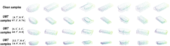
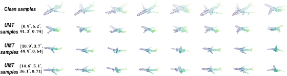
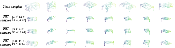
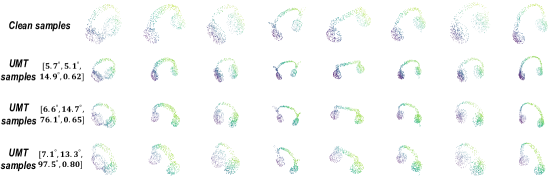
Visual Effect. We visualize UMT samples in Figs. 7, 8, 9 and 10, indicating that the unlearnable point cloud samples still retain their normal feature structure with visual rationality.
Evaluation of Semantic Segmentation. We evaluate UMT using common metrics for point cloud semantic segmentation tasks in Tab. 3. As can be seen, the performance of semantic segmentation of data protected by UMT significantly decreases. The underlying reason is that the DNNs learn the features of class-wise transformations and establish a new mapping, which leads to the inability of test samples without transformations to be correctly segmented by the segmentation model.
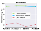
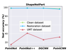
Evaluation of Data Restoration. We multiply UMT samples by the transformation matrix in Eq. 9. The data becomes learnable after the restoration process, with test accuracy reaching a level comparable to the clean baseline as shown in Fig. 4. This strongly validates the effectiveness of the proposed data restoration scheme.
| Datasets | Modules Models | PointNet | PointNet++ | DGCNN | PointCNN | CurveNet | SimpleView | RIConv | LGR-Net | 3DGCN | PointNN | PointMLP | AVG |
|---|---|---|---|---|---|---|---|---|---|---|---|---|---|
| ModelNet40 | Module | 27.19 | 20.02 | 28.61 | 21.64 | 36.87 | 28.32 | 88.25 | 40.24 | 24.59 | 28.77 | 27.72 | 33.84 |
| Module | 9.36 | 48.70 | 15.07 | 7.41 | 13.92 | 20.33 | 32.25 | 12.56 | 88.72 | 65.32 | 18.79 | 30.22 | |
| UMT(k=2) | 9.20 | 18.52 | 13.86 | 9.08 | 13.90 | 7.58 | 24.39 | 9.85 | 26.58 | 25.12 | 7.31 | 15.04 | |
| ModelNet10 | Module | 29.85 | 30.51 | 35.13 | 31.17 | 47.25 | 58.70 | 91.38 | 43.72 | 36.50 | 34.58 | 30.47 | 42.66 |
| Module | 34.80 | 57.05 | 42.62 | 33.81 | 30.36 | 43.75 | 42.24 | 32.60 | 89.40 | 73.79 | 41.29 | 47.43 | |
| UMT(k=2) | 22.25 | 28.08 | 14.10 | 21.48 | 24.34 | 21.37 | 38.18 | 19.82 | 31.28 | 33.37 | 29.35 | 25.78 |
4.3 Ablation Study and Hyper-Parameter Sensitivity Analysis
Ablation on Rotation Module. As shown in Tab. 4, the average accuracy increases by 15.18% and 21.65%, respectively, when only using . This suggests the importance of class-wise rotation module. The high test accuracy demonstrated by 3DGCN [24] can be attributed to its scaling invariance, which endows it with robustness against scaling transformation.
Ablation on Scaling Module. As also shown in Tab. 4, the average accuracy increases by 18.80% and 16.88% when only using the rotation module, respectively. The high test accuracy achieved on RIConv [55] and LGR-Net [57] is due to the fact that both networks are rotation-invariant, thus providing resistance against rotation transformations. These ablation results furthermore emphasize the importance of incorporating more non-rigid transformations.
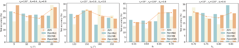
Hyper-Parameter Analysis. We analyze four hyperparameters , , , and in Fig. 5. The influence of and on the accuracy remains relatively small, exhibiting their best unlearnable effect when set to 15∘ and 120∘, respectively. We attribute this to the crucial role played by the class-wise setting, while it is not highly sensitive to the size of specific values. The unlearnable effect is the best when and are set to 0.6 and 0.8, respectively. Similarly, the variations in and do not significantly alter the effect due to the class-wise setting.
4.4 Insightful Analysis Into UMT
We formalize , where is the cross-entropy loss, is the point cloud data sampled from dataset . We define , , and as the training set, unlearnable test set (i.e., test set transformed by UMT), and clean test set, respectively. Thus we have the training loss , unlearnable test loss , and clean test loss .
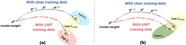
The models trained on both clean and UMT training sets exhibit low as shown in Fig. 6 (yellow ellipses), indicating the models converge well during training. Furthermore, when tested on as shown in Fig. 6 (a), the clean model (trained with clean training set) achieves a low (blue ellipse), while the UMT model (trained with UMT training set) exhibits a high (red ellipse), also supporting the unlearnable effectiveness of UMT. Fig. 6 (b) reveals that the clean model and UMT model both exhibit low (green ellipse), suggesting that they can classify UMT samples. But the mechanisms underlying the two cases of low differ. The clean one is due to that the semantics of samples can be remained by UMT and thus normally classified. The UMT one is that the UMT model learns the mapping between transformations and labels, thereby correctly predicting the samples containing the same transformations. We conclude that the clean model effectively classifies both clean and UMT samples, while the UMT model successfully classifies UMT samples (the UMT process is the same for both training and test samples) but fails to classify clean samples.
5 Related Work
5.1 2D Unlearnable Schemes
The development of 2D unlearnable schemes [17, 27, 35, 37, 40, 53] has been booming. Specifically, model-dependent methods are initially proposed in abundance [8, 17, 27]. Afterwards, numerous model-agnostic methods that significantly improve the generation efficiency have surfaced [37, 40, 45]. However, due to the structural disparities between 3D point cloud data and 2D images, applying unlearnable methods directly from 2D to 3D reveals significant challenges.
5.2 Protecting 3D Point Cloud Data Privacy
Some works proposed an encryption scheme based on chaotic mapping [19] or optical chaotic encryption [25], and a 3D object reconstruction technique was introduced [32], both achieving privacy protection for individual 3D point cloud data. Nevertheless, no privacy-preserving solution has been proposed specifically for the scenario of unauthorized DNN learning on abundant raw 3D point cloud data. It is worth mentioning that both parallel works [42, 61] studied availability poisoning attacks against 3D point cloud networks, which largely reduce model accuracy, and both have the potential to be applied as unlearnable schemes. However, the feature collision error-minimization poisoning scheme proposed by Zhu et al. [61] overlooks the problem of effective training for authorized users, which limits its practical use in real-world applications. The rotation-based poisoning approach proposed by Wang et al. [42] is easily defeated by rotation-invariant networks [55, 56, 57], as revealed in Tabs. 1 and 4.
6 Conclusion, Limitation, and Broader Impacts
In this research, we propose the first integral unlearnable framework in 3D point clouds, which utilizes class-wise multi transformations, preventing unauthorized deep learning while allowing authorized training. Extensive experiments on synthetic and real-world datasets and theoretical evidence verify the superiority of our framework. The transformations include rotation, scaling, twisting, and shear, which are all common 3D transformation operations. If unauthorized users design a network that is invariant to all these transformations, they could potentially defeat our proposed UMT. So far, only networks invariant to rigid transformations like rotation and scaling have been proposed, while networks invariant to non-rigid transformations like twisting and shear, have not yet been introduced. Therefore, our research also contributes to the design of more transformation-invariant networks.
Our research calls for the design of more robust point cloud networks, which helps improve the robustness and security of 3D point cloud processing systems. On the other hand, if our proposed UMT scheme is maliciously exploited, it may have negative impacts on society, such as causing a sharp decline in the performance of models trained on it, affecting the security and reliability of technologies based on 3D point cloud networks. More transformation-invariant 3D point cloud networks need to be proposed in the future to avoid potential negative impacts.
References
- [1] Evangelos Alexiou, Nanyang Yang, and Touradj Ebrahimi. Pointxr: A toolbox for visualization and subjective evaluation of point clouds in virtual reality. In Proceedings of the 12th International Conference on Quality of Multimedia Experience (QoMEX’20), pages 1–6, 2020.
- [2] Iro Armeni, Ozan Sener, Amir R Zamir, Helen Jiang, Ioannis Brilakis, Martin Fischer, and Silvio Savarese. 3d semantic parsing of large-scale indoor spaces. In Proceedings of the 2016 IEEE Conference on Computer Vision and Pattern Recognition (CVPR’16), pages 1534–1543, 2016.
- [3] Angel X. Chang, Thomas Funkhouser, Leonidas Guibas, Pat Hanrahan, Qixing Huang, Zimo Li, Silvio Savarese, Manolis Savva, Shuran Song, Hao Su, et al. Shapenet: An information-rich 3d model repository. arXiv preprint arXiv:1512.03012, 2015.
- [4] Sizhe Chen, Geng Yuan, Xinwen Cheng, Yifan Gong, Minghai Qin, Yanzhi Wang, and Xiaolin Huang. Self-ensemble protection: Training checkpoints are good data protectors. In Proceedings of the 11th International Conference on Learning Representations (ICLR’23), 2023.
- [5] Xiaozhi Chen, Huimin Ma, Ji Wan, Bo Li, and Tian Xia. Multi-view 3d object detection network for autonomous driving. In Proceedings of the 2017 IEEE Conference on Computer Vision and Pattern Recognition (CVPR’17), pages 1907–1915, 2017.
- [6] Wenda Chu, Linyi Li, and Bo Li. Tpc: Transformation-specific smoothing for point cloud models. In Proceedings of the 39th International Conference on Machine Learning (ICML’22), pages 4035–4056, 2022.
- [7] Liam Fowl, Micah Goldblum, Ping-yeh Chiang, Jonas Geiping, Wojciech Czaja, and Tom Goldstein. Adversarial examples make strong poisons. In Proceedings of the 35th Neural Information Processing Systems (NeurIPS’21), pages 30339–30351, 2021.
- [8] Shaopeng Fu, Fengxiang He, Yang Liu, Li Shen, and Dacheng Tao. Robust unlearnable examples: Protecting data against adversarial learning. In Proceedings of the 10th International Conference on Learning Representations (ICLR’22), 2022.
- [9] Fabian Fuchs, Daniel Worrall, Volker Fischer, and Max Welling. SE (3)-transformers: 3D roto-translation equivariant attention networks. In Proceedings of the 34th Neural Information Processing Systems (NeurIPS’20), volume 33, pages 1970–1981, 2020.
- [10] Cong Gao, Geng Wang, Weisong Shi, Zhongmin Wang, and Yanping Chen. Autonomous driving security: State of the art and challenges. IEEE Internet of Things Journal, 9(10):7572–7595, 2021.
- [11] Kuofeng Gao, Jiawang Bai, Baoyuan Wu, Mengxi Ya, and Shu-Tao Xia. Imperceptible and robust backdoor attack in 3d point cloud. IEEE Transactions on Information Forensics and Security (TIFS’23), 19:1267–1282, 2023.
- [12] Robert Geirhos, Jörn-Henrik Jacobsen, Claudio Michaelis, Richard Zemel, Wieland Brendel, Matthias Bethge, and Felix A Wichmann. Shortcut learning in deep neural networks. Nature Machine Intelligence, pages 665–673, 2020.
- [13] Ankit Goyal, Hei Law, Bowei Liu, Alejandro Newell, and Jia Deng. Revisiting point cloud shape classification with a simple and effective baseline. In Proceedings of the 38th International Conference on Machine Learning (ICML’21), pages 3809–3820. PMLR, 2021.
- [14] Meng-Hao Guo, Jun-Xiong Cai, Zheng-Ning Liu, Tai-Jiang Mu, Ralph R Martin, and Shi-Min Hu. Pct: Point cloud transformer. Computational Visual Media, 7:187–199, 2021.
- [15] Shengshan Hu, Wei Liu, Minghui Li, Yechao Zhang, Xiaogeng Liu, Xianlong Wang, Leo Yu Zhang, and Junhui Hou. Pointcrt: Detecting backdoor in 3d point cloud via corruption robustness. In Proceedings of the 31st ACM International Conference on Multimedia (MM’23), pages 666–675, 2023.
- [16] Shengshan Hu, Junwei Zhang, Wei Liu, Junhui Hou, Minghui Li, Leo Yu Zhang, Hai Jin, and Lichao Sun. Pointca: Evaluating the robustness of 3d point cloud completion models against adversarial examples. In Proceedings of the 37th AAAI Conference on Artificial Intelligence (AAAI’23), pages 872–880, 2023.
- [17] Hanxun Huang, Xingjun Ma, Sarah Monazam Erfani, James Bailey, and Yisen Wang. Unlearnable examples: Making personal data unexploitable. In Proceedings of the 9th International Conference on Learning Representations (ICLR’21), 2021.
- [18] Adel Javanmard and Mahdi Soltanolkotabi. Precise statistical analysis of classification accuracies for adversarial training. The Annals of Statistics, 50(4):2127–2156, 2022.
- [19] Xin Jin, Zhaoxing Wu, Chenggen Song, Chunwei Zhang, and Xiaodong Li. 3d point cloud encryption through chaotic mapping. In Proceedings of the 17th Pacific Rim Conference on Multimedia (PCM’16), pages 119–129, 2016.
- [20] Diederik P Kingma and Jimmy Ba. Adam: A method for stochastic optimization. arXiv preprint arXiv:1412.6980, 2014.
- [21] Peiliang Li, Siqi Liu, and Shaojie Shen. Multi-sensor 3d object box refinement for autonomous driving. arXiv preprint arXiv:1909.04942, 2019.
- [22] Xinke Li, Zhirui Chen, Yue Zhao, Zekun Tong, Yabang Zhao, Andrew Lim, and Joey Tianyi Zhou. Pointba: Towards backdoor attacks in 3d point cloud. In Proceedings of the 18th IEEE/CVF International Conference on Computer Vision (ICCV’21), pages 16492–16501, 2021.
- [23] Yangyan Li, Rui Bu, Mingchao Sun, Wei Wu, Xinhan Di, and Baoquan Chen. Pointcnn: Convolution on x-transformed points. In Proceedings of the 32nd Neural Information Processing Systems (NeurIPS’18), pages 828–838, 2018.
- [24] Zhi-Hao Lin, Sheng-Yu Huang, and Yu-Chiang Frank Wang. Convolution in the cloud: Learning deformable kernels in 3d graph convolution networks for point cloud analysis. In Proceedings of the 2020 IEEE/CVF Conference on Computer Vision and Pattern Recognition (CVPR’20), pages 1800–1809, 2020.
- [25] Bocheng Liu, Yongxiang Liu, Yiyuan Xie, Xiao Jiang, Yichen Ye, Tingting Song, Junxiong Chai, Meng Liu, Manying Feng, and Haodong Yuan. Privacy protection for 3d point cloud classification based on an optical chaotic encryption scheme. Optics Express, 31(5):8820–8843, 2023.
- [26] Shuang Liu, Yihan Wang, and Xiao-Shan Gao. Game-theoretic unlearnable example generator. In Proceedings of the AAAI Conference on Artificial Intelligence (AAAI’24), 2024.
- [27] Yixin Liu, Kaidi Xu, Xun Chen, and Lichao Sun. Stable unlearnable example: Enhancing the robustness of unlearnable examples via stable error-minimizing noise. In Proceedings of the AAAI Conference on Artificial Intelligence (AAAI’24), pages 3783–3791, 2024.
- [28] Ilya Loshchilov and Frank Hutter. Sgdr: Stochastic gradient descent with warm restarts. arXiv preprint arXiv:1608.03983, 2016.
- [29] Xu Ma, Can Qin, Haoxuan You, Haoxi Ran, and Yun Fu. Rethinking network design and local geometry in point cloud: A simple residual mlp framework. arXiv preprint arXiv:2202.07123, 2022.
- [30] Moritz Menze and Andreas Geiger. Object scene flow for autonomous vehicles. In Proceedings of the 2015 IEEE Conference on Computer Vision and Pattern Recognition (CVPR’15), pages 3061–3070, 2015.
- [31] Yifei Min, Lin Chen, and Amin Karbasi. The curious case of adversarially robust models: More data can help, double descend, or hurt generalization. In Uncertainty in Artificial Intelligence, pages 129–139. PMLR, 2021.
- [32] Arpit Nama, Amaya Dharmasiri, Kanchana Thilakarathna, Albert Zomaya, and Jaybie Agullo de Guzman. User configurable 3d object regeneration for spatial privacy. arXiv preprint arXiv:2108.08273, 2021.
- [33] Charles Ruizhongtai Qi, Hao Su, Kaichun Mo, and Leonidas J. Guibas. Pointnet: Deep learning on point sets for 3d classification and segmentation. In Proceedings of the 2017 IEEE Conference on Computer Vision and Pattern Recognition (CVPR’17), pages 652–660, 2017.
- [34] Charles Ruizhongtai Qi, Li Yi, Hao Su, and Leonidas J. Guibas. Pointnet++: Deep hierarchical feature learning on point sets in a metric space. In Proceedings of the 31st Neural Information Processing Systems (NeurIPS’17), pages 5099–5108, 2017.
- [35] Jie Ren, Han Xu, Yuxuan Wan, Xingjun Ma, Lichao Sun, and Jiliang Tang. Transferable unlearnable examples. In Proceedings of the 11th International Conference on Learning Representations (ICLR’23), 2023.
- [36] Douglas A Reynolds et al. Gaussian mixture models. Encyclopedia of biometrics, 741(659-663), 2009.
- [37] Vinu Sankar Sadasivan, Mahdi Soltanolkotabi, and Soheil Feizi. CUDA: Convolution-based unlearnable datasets. In Proceedings of the IEEE/CVF Conference on Computer Vision and Pattern Recognition (CVPR’23), pages 3862–3871, 2023.
- [38] StubbornAtom. Distributions of quadratic form of a normal random variable. Cross Validated, 2020. (version: 2020-07-23).
- [39] Mikaela Angelina Uy, Quang-Hieu Pham, Binh-Son Hua, Duc Thanh Nguyen, and Sai-Kit Yeung. Revisiting point cloud classification: A new benchmark dataset and classification model on real-world data. In Proceedings of the 17th IEEE/CVF International Conference on Computer Vision (ICCV’19), 2019.
- [40] Xianlong Wang, Shengshan Hu, Minghui Li, Zhifei Yu, Ziqi Zhou, and Leo Yu Zhang. Corrupting convolution-based unlearnable datasets with pixel-based image transformations. arXiv preprint arXiv:2311.18403, 2023.
- [41] Xianlong Wang, Shengshan Hu, Yechao Zhang, Ziqi Zhou, Leo Yu Zhang, Peng Xu, Wei Wan, and Hai Jin. ECLIPSE: Expunging clean-label indiscriminate poisons via sparse diffusion purification. In Proceedings of the 29th European Symposium on Research in Computer Security (ESORICS’24), pages 146–166, 2024.
- [42] Xianlong Wang, Minghui Li, Peng Xu, Wei Liu, Leo Yu Zhang, Shengshan Hu, and Yanjun Zhang. PointAPA: Towards availability poisoning attacks in 3D point clouds. In Proceedings of the 29th European Symposium on Research in Computer Security (ESORICS’24), pages 125–145, 2024.
- [43] Yue Wang, Yongbin Sun, Ziwei Liu, Sanjay E. Sarma, Michael M. Bronstein, and Justin M. Solomon. Dynamic graph cnn for learning on point clouds. ACM Transactions On Graphics (TOG’19), pages 1–12, 2019.
- [44] Florian Wirth, Jannik Quehl, Jeffrey Ota, and Christoph Stiller. Pointatme: efficient 3d point cloud labeling in virtual reality. In Proceedings of the 2019 IEEE Intelligent Vehicles Symposium (IV’19), pages 1693–1698, 2019.
- [45] Shutong Wu, Sizhe Chen, Cihang Xie, and Xiaolin Huang. One-pixel shortcut: on the learning preference of deep neural networks. In Proceedings of the 11th International Conference on Learning Representations (ICLR’23), 2023.
- [46] Wenxuan Wu, Zhongang Qi, and Li Fuxin. Pointconv: Deep convolutional networks on 3d point clouds. In Proceedings of the 2019 IEEE/CVF Conference on Computer Vision and Pattern Recognition (CVPR’19), pages 9621–9630, 2019.
- [47] Xiaoyang Wu, Li Jiang, Peng-Shuai Wang, Zhijian Liu, Xihui Liu, Yu Qiao, Wanli Ouyang, Tong He, and Hengshuang Zhao. Point transformer v3: Simpler, faster, stronger. arXiv preprint arXiv:2312.10035, 2023.
- [48] Zhirong Wu, Shuran Song, Aditya Khosla, Fisher Yu, Linguang Zhang, Xiaoou Tang, and Jianxiong Xiao. 3d shapenets: A deep representation for volumetric shapes. In Proceedings of the 2015 IEEE Conference on Computer Vision and Pattern Recognition (CVPR’15), pages 1912–1920, 2015.
- [49] Tiange Xiang, Chaoyi Zhang, Yang Song, Jianhui Yu, and Weidong Cai. Walk in the cloud: Learning curves for point clouds shape analysis. In Proceedings of the 18th IEEE/CVF International Conference on Computer Vision (ICCV’21), pages 915–924, 2021.
- [50] Zhen Xiang, David J. Miller, Siheng Chen, Xi Li, and George Kesidis. A backdoor attack against 3d point cloud classifiers. In Proceedings of the 18th IEEE/CVF International Conference on Computer Vision (ICCV’21), pages 7597–7607, 2021.
- [51] Jiancheng Yang, Qiang Zhang, Rongyao Fang, Bingbing Ni, Jinxian Liu, and Qi Tian. Adversarial attack and defense on point sets. arXiv preprint arXiv:1902.10899, 2019.
- [52] Jingwen Ye and Xinchao Wang. Ungeneralizable examples. In Proceedings of the 2024 IEEE Conference on Computer Vision and Pattern Recognition (CVPR’24), 2024.
- [53] Jiaming Zhang, Xingjun Ma, Qi Yi, Jitao Sang, Yugang Jiang, Yaowei Wang, and Changsheng Xu. Unlearnable clusters: Towards label-agnostic unlearnable examples. In Proceedings of the 2023 IEEE/CVF Conference on Computer Vision and Pattern Recognition (CVPR’23), 2023.
- [54] Renrui Zhang, Liuhui Wang, Yali Wang, Peng Gao, Hongsheng Li, and Jianbo Shi. Parameter is not all you need: Starting from non-parametric networks for 3d point cloud analysis. arXiv preprint arXiv:2303.08134, 2023.
- [55] Zhiyuan Zhang, Binh-Son Hua, David W Rosen, and Sai-Kit Yeung. Rotation invariant convolutions for 3d point clouds deep learning. In Proceedings of the 2019 International Conference on 3D Vision (3DV’19), pages 204–213. IEEE, 2019.
- [56] Zhiyuan Zhang, Binh-Son Hua, and Sai-Kit Yeung. Riconv++: Effective rotation invariant convolutions for 3d point clouds deep learning. International Journal of Computer Vision (IJCV’22), 130(5):1228–1243, 2022.
- [57] Chen Zhao, Jiaqi Yang, Xin Xiong, Angfan Zhu, Zhiguo Cao, and Xin Li. Rotation invariant point cloud classification: Where local geometry meets global topology. arXiv preprint arXiv:1911.00195, 2019.
- [58] Hang Zhou, Kejiang Chen, Weiming Zhang, Han Fang, Wenbo Zhou, and Nenghai Yu. Dup-net: Denoiser and upsampler network for 3D adversarial point clouds defense. In Proceedings of the 17th IEEE/CVF International Conference on Computer Vision (ICCV’19), pages 1961–1970, 2019.
- [59] Ziqi Zhou, Yufei Song, Minghui Li, Shengshan Hu, Xianlong Wang, Leo Yu Zhang, Dezhong Yao, and Hai Jin. Darksam: Fooling segment anything model to segment nothing. arXiv preprint arXiv:2409.17874, 2024.
- [60] Xiangyang Zhu, Renrui Zhang, Bowei He, Ziyu Guo, Jiaming Liu, Han Xiao, Chaoyou Fu, Hao Dong, and Peng Gao. No time to train: Empowering non-parametric networks for few-shot 3d scene segmentation. In Proceedings of the 2024 IEEE Conference on Computer Vision and Pattern Recognition (CVPR’24), 2024.
- [61] Yifan Zhu, Yibo Miao, Yinpeng Dong, and Xiao-Shan Gao. Toward availability attacks in 3D point clouds. arXiv preprint arXiv:2407.11011, 2024.
Appendix: Unlearnable 3D Point Clouds: Class-wise Transformation Is All You Need
Appendix A Definitions of 3D Transformations
Existing 3D transformations are summarized in Fig. 1 and formally defined in this section. The 3D transformations are mathematical operations applied to three-dimensional objects to change their position, orientation, and scale in space, which are often represented using transformation matrices. We formally define the transformed point cloud sample with transformation matrix as:
| (10) |
where is the clean point cloud sample, is the transformed point cloud sample.
A.1 Rotation Transformation
The rotation transformation that alters the orientation and angle of 3D point clouds is controlled by three angles , , and . The rotation matrices in three directions can be formally defined as:
| (11) |
Thus we have while employing rotation transformation. Besides, we have , , and .
A.2 Scaling Transformation
The scaling matrix can be represented as:
| (12) |
where the scaling factor is used to perform a proportional scaling of the coordinates of each point in the point cloud.
A.3 Shear Transformation
In the three-dimensional space, shearing 222https://www.mauriciopoppe.com/notes/computer-graphics/transformation-matrices/shearing/ is represented by different matrices, and the specific form depends on the type of shear being performed. Specifically, the shear transformation matrix (employed in UMT) of shifting and by the other coordinate , and its corresponding inverse matrix can be expressed as:
| (13) |
The shear transformation matrix of shifting and by the other coordinate , and its corresponding inverse matrix can be expressed as:
| (14) |
And the shear transformation matrix of shifting and by the other coordinate , and its corresponding inverse matrix can be expressed as:
| (15) |
Input: Clean 3D point cloud dataset ; number of categories ; slight range ; primary range ; scaling lower bound ; scaling upper bound ;
twisting lower bound ; twisting upper bound ;
shear lower bound ; shear upper bound ;
spectrum of transformations ; matrix set .
Output: Unlearnable 3D point cloud dataset .
Initialize the slight angle lists =[ ], =[ ], the primary angle list =[ ], the rotation list =[ ], the scaling list =[ ], the twisting list =[ ], the shear list =[ ], and ;
for to do
Add to the list ;
Add to the list ;
Add to the list ;
Get the transformed data ;
A.4 Twisting Transformation
The 3D twisting transformation [6] involves a rotational deformation applied to an object in three-dimensional space, creating a twisted or spiraled effect. Unlike simple rotations around fixed axes, a twisting transformation introduces a variable rotation that may change based on the spatial coordinates of the object. For instance, considering a twisting transformation along the -axis, where the rotation angle is a function related to the -coordinate, it can be expressed as:
| (16) |
where is the parameter of the twisting transformation, and is the -coordinate of the object. The inverse matrix of is:
| (17) |
A.5 Tapering Transformation
The tapering transformation [6] is a linear transformation used to alter the shape of an object, causing it to gradually become pointed or shortened. In three-dimensional space, tapering transformation can adjust the dimensions of an object along one or more axes, creating a tapering effect. The specific matrix representation of tapering transformation depends on the chosen axis and the design of the transformation. Generally, tapering transformation can be represented by a matrix that is multiplied by the coordinates of the object to achieve the shape adjustment, which is defined as:
| (18) |
where is the -coordinate of the object. Considering that could indeed equal -1, in such a case, the 3D point cloud samples would be projected onto the -plane, losing their practical significance and the tapering matrix is also irreversible.
A.6 Reflection Transformation
Reflection transformation is a linear transformation that inverts an object along a certain plane. This plane is commonly referred to as a reflection plane or mirror. For reflection transformations in three-dimensional space, we can represent them through a matrix. Regarding the reflection transformation matrices of the plane, plane, and plane, we have:
| (19) |
A.7 Translation Transformation
The 3D translation transformation333https://www.javatpoint.com/computer-graphics-3d-transformations refers to the process of moving an object in three-dimensional space. This transformation involves moving the object along the , , and axes, respectively, smoothly transitioning it from one position to another, which is defined as:
| (20) |
where , , and represents the translation along the , , and axes, respectively. This 44 matrix is a homogeneous coordinate matrix that describes the translation in three-dimensional space. Additionally, the translation matrix also can be represented as a additive matrix to original point , which can be defined as:
| (21) |
Appendix B Supplementary Experimental Settings
B.1 Experimental Platform
Our experiments are conducted on a server running a 64-bit Ubuntu 20.04.1 system with an Intel(R) Xeon(R) Silver 4210R CPU @ 2.40GHz processor, 125GB memory, and four Nvidia GeForce RTX 3090 GPUs, each with 24GB memory. The experiments are performed using the Python language, version 3.8.19, and PyTorch library version 1.12.1.
B.2 Hyper-Parameter Settings
The model training process on the unlearnable dataset and the clean dataset remains consistent, using the Adam optimizer [20], CosineAnnealingLR scheduler [28], initial learning rate of 0.001, weight decay of 0.0001, batch size of 16 (due to insufficient GPU memory, the batch size is set to 8 when training 3DGCN on ModelNet40 dataset), and training for 80 epochs. Due to the longer training process required by PCT [14], the training epochs for PCT in Tab. 1 on ModelNet10, ModelNet40, and ScanObjectNN datasets are all set to 240.
B.3 Settings of Exploring Experiments
| Transformations | Rotation | Scaling | Shear | Twisting | Tapering | Translation | AVG |
|---|---|---|---|---|---|---|---|
| w/o | 89.32 | 89.32 | 89.32 | 89.32 | 89.32 | 89.32 | 89.32 |
| Sample-wise | 91.52 | 87.78 | 89.10 | 92.62 | 90.31 | 90.31 | 89.80 |
| Dataset-wise | 87.89 | 79.41 | 85.79 | 92.18 | 88.22 | 88.22 | 83.45 |
| Class-wise | 29.85 | 20.81 | 67.84 | 63.22 | 52.42 | 36.67 | 45.14 |
| Test sets Transformations | Rotation | Scaling | Shear | Twisting | Tapering | Translation |
|---|---|---|---|---|---|---|
| Class-wise test set | 99.67 | 93.80 | 97.91 | 94.05 | 96.04 | 98.24 |
| Permuted class-wise test set | 10.68 | 38.22 | 58.37 | 60.68 | 42.51 | 31.94 |
| Clean test set | 29.85 | 20.81 | 67.84 | 63.22 | 52.42 | 36.67 |
We initially investigate which approach yields the best unlearnable effect among sample-wise, dataset-wise, and class-wise settings in Fig. 2 (a). Specific experimental settings are as follows:
In the dataset-wise setting, the same parameter values are applied to the entire dataset. Specifically, we have in the rotation transformation, the scaling factor is set to 0.8, both shearing factors and are set to 0.2. The angle in twisting is . The tapering angle is set to , and the parameters in translation transformation , , and are set to 0.15.
In the sample-wise setting, each sample has its independent set of parameters, meaning the parameter values for each sample are randomly generated within a certain range. In the rotation transformation, , , are uniformly sampled from the range of to . The scaling factor is uniformly sampled from 0.6 to 0.8, shearing factors and are uniformly sampled from the range of 0 to 0.4. Both the twist angle and tapering angle are sampled from to , and the parameters in translation transformation , , and are sampled from 0 to 0.3.
In the class-wise setting, the parameters for transformations are associated with the point cloud’s class. The selection of parameters for each class is also obtained by random sampling within a fixed range. The chosen ranges are generally consistent with those described for the sample-wise setting above. However, a difference lies in the consideration of slight angle range and primary angle range in the case of rotation transformations, where these ranges are and , respectively.
The specific results of test accuracy under different transformation modes, including sample-wise (random), class-wise, and dataset-wise (universal), are provided in Tab. 5. It can be seen that under the class-wise setting, the final unlearnable effect is the best.
B.4 Benchmark Datasets
Dataset introduction. The ModelNet40 dataset is a point cloud dataset containing 40 categories, comprising 9843 training and 2468 test point cloud data. ModelNet10 is a subset of ModelNet40 dataset with 10 categories. ShapeNetPart that includes 16 categories is a subset of ShapeNet, comprising 12137 training and 2874 test point cloud samples. ScanObjectNN is a real-world point cloud dataset with 15 categories, comprising 2309 training samples and 581 test samples. Similar to [50, 15], we split KITTI object clouds into class “vehicle” and “human” containing 1000 training data and 662 test data. The input point cloud objects for the models encompass 256 points for the KITTI dataset and 1024 points for other datasets. The Stanford 3D Indoor Scene Dataset (S3DIS) dataset contains 6 large-scale indoor areas with 271 rooms. Each point in the scene point cloud is annotated with one of the 13 semantic categories.
Dataset licenses. The dataset license information is listed as:
-
•
ModelNet10, ModelNet40 [48]: All CAD models are downloaded from the Internet and the original authors hold the copyright of the CAD models. The label of the data was obtained by us via Amazon Mechanical Turk service and it is provided freely. This dataset is provided for the convenience of academic research only. Link is https://modelnet.cs.princeton.edu/.
-
•
ShapeNetPart [3]: We use the ShapeNet database (the "Database") at Princeton University and Stanford University. Link is https://www.shapenet.org/.
-
•
ScanObjectNN [39]: The license is MIT License: Copyright (c) 2019 Vision & Graphics Group, HKUST. Permission is hereby granted, free of charge, to any person obtaining a copy of this software and associated documentation files (the "Software"), to deal in the Software without restriction, including without limitation the rights to use, copy, modify, merge, publish, distribute, sublicense, and/or sell copies of the Software, and to permit persons to whom the Software is furnished to do so, subject to the following conditions: The above copyright notice and this permission notice shall be included in all copies or substantial portions of the Software. Link is https://hkust-vgd.github.io/scanobjectnn/.
-
•
S3DIS [2]: The copyright is from Stanford University, Patent Pending, copyright 2016. Link is http://buildingparser.stanford.edu/dataset.html.
B.5 Settings of Robustness Experiments
The scaling factor in random scaling augmentation is set to a minimum of 0.8 and a maximum of 1.25. In the random rotation operation, the three directional rotation angles are identical and uniformly sampled from [0, 2). The perturbations in the random jitter are sampled from a normal distribution with a standard deviation of 0.05, and the perturbation magnitude is constrained within 0.1. The parameters and in SOR are set to 2 and 1.1, respectively. The number of dropped points in SRS is 500.
Appendix C Supplementary Experimental Results
C.1 Results for Execution Mechanism
We present the specific experimental results of Fig. 2 (a) in Tab. 5. It can be observed that under the class-wise setting, the average test accuracy is the lowest, while the unlearnable condition yields the best performance. Furthermore, we conduct investigations into training the PointNet classifier with class-wise transformed training sets (ModelNet10 dataset), analyzing accuracy results across different test sets, as shown in Tab. 6. It is noteworthy that the accuracy on class-wise test sets (using consistent transformation parameters with class-wise transformed training set) is consistently above 90%, indicating that the model has learned the mapping between transformations and labels. This leads to correct classification on test samples with the same transformations. However, when the class-wise test set undergoes permutation, the accuracy drops to a level similar to that of the clean test set. This clearly demonstrates that the model can correctly classify samples only when they have corresponding transformations, and samples without transformations or with mismatched transformations cannot be correctly classified. This further validates that the model learns a one-to-one mapping between class transformations and labels.
C.2 Results of Diverse Combinations of Transformations
We investigate combinations of four transformations, i.e., rotation, scaling, shear, and twisting, and create unlearnable datasets using the class-wise setting. The test accuracy results across five point cloud models are presented in Tab. 7. It can be observed that the combination of rotation and scaling, two types of rigid transformations, achieves the most effective unlearnable effect. The transformation parameters used in this section are consistent with Sec. B.3.
| Transformations | PointNet | PointNet++ | DGCNN | PointCNN | PCT | AVG |
|---|---|---|---|---|---|---|
| 46.70 | 38.99 | 49.67 | 64.87 | 27.53 | 45.55 | |
| 34.80 | 57.05 | 42.62 | 33.81 | 29.63 | 39.58 | |
| 64.10 | 66.41 | 71.15 | 60.68 | 60.13 | 64.49 | |
| 76.98 | 54.19 | 78.63 | 86.69 | 38.55 | 67.05 | |
| 22.25 | 28.08 | 14.10 | 21.48 | 11.89 | 19.56 | |
| 30.51 | 39.98 | 45.93 | 36.23 | 33.81 | 37.29 | |
| 34.91 | 44.27 | 29.52 | 46.92 | 32.16 | 37.56 | |
| 20.26 | 44.93 | 38.66 | 43.50 | 34.80 | 36.43 | |
| 18.28 | 44.27 | 31.39 | 34.25 | 19.93 | 29.62 | |
| 63.33 | 62.56 | 61.89 | 64.76 | 51.43 | 60.79 | |
| 15.97 | 29.19 | 36.56 | 21.81 | 31.28 | 26.96 | |
| 25.22 | 31.50 | 23.57 | 31.83 | 38.55 | 30.13 | |
| 21.70 | 46.37 | 55.29 | 37.11 | 38.77 | 39.85 | |
| 16.52 | 33.37 | 30.51 | 30.73 | 32.49 | 28.72 |
| Training and test sets | PointNet | PointNet++ | DGCNN | PointCNN | AVG |
|---|---|---|---|---|---|
| Clean training set, clean test set | 89.32 | 92.95 | 92.73 | 89.54 | 91.14 |
| Clean training set, UMT test set | 55.51 | 70.93 | 74.78 | 69.71 | 67.73 |
| UMT training set, clean test set | 22.25 | 28.08 | 14.10 | 21.48 | 21.48 |
| UMT training set, UMT test set | 98.79 | 99.23 | 99.01 | 96.26 | 98.32 |
C.3 More Results of UMT Against Adaptive Attacks
To further explore the performance of UMT against adaptive attacks, we supplement the experimental results using four types of random augmentations in Tab. 9, and find that the conclusion is consistent with Tab. 2.
| ModelNet10 | PointNet | PointNet++ | DGCNN | PointCNN | AVG |
|---|---|---|---|---|---|
| Clean baseline | 89.32 | 92.95 | 92.73 | 89.54 | 91.14 |
| UMT(k=4) | 16.19 | 36.56 | 17.62 | 27.42 | 24.45 |
| UMT(k=4) + random | 25.99 | 61.78 | 61.89 | 44.16 | 48.46 |
C.4 Results of Insightful Analysis
We train on clean training set and test on clean test set, train on clean training set and test on UMT test set, train on UMT training set and test on clean test set, and train on UMT training set and test on UMT test set to obtain the test accuracy results in Tab. 8 (we ensure that the UMT parameters for the UMT test set and UMT training set are consistent). Higher accuracy values indicate lower cross-entropy loss values, while lower accuracy values represent higher cross-entropy loss values. It can be observed that only when trained with the UMT training set, the loss after testing with the clean test set is high (i.e., low accuracy).
C.5 Boarder Hyper-Parameter Analysis
Additionally, we investigate the unlearnable effects across a wider range of hype-parameters in UMT ( with ), as shown in Tab. 10. It can be observed that our UMT scheme still exhibits a good unlearnable effect, and its key lies in the crucial role played by the class-wise setting.
| , , , | PointNet | DGCNN | PointCNN | AVG | , , , | PointNet | DGCNN | PointCNN | AVG |
|---|---|---|---|---|---|---|---|---|---|
| 25, 120, 0.6, 0.8 | 24.78 | 23.35 | 28.19 | 25.44 | 15, 120, 0.75, 0.8 | 154 | 38.66 | 40.09 | 31.10 |
| 25, 180, 0.6, 0.8 | 26.65 | 25.99 | 20.37 | 234 | 15, 120, 0.6, 0.7 | 20.59 | 27.53 | 23.68 | 23.93 |
| 15, 90, 0.6, 0.8 | 18.39 | 20.59 | 22.03 | 20.34 | 15, 120, 0.6, 0.8 | 22.25 | 14.10 | 21.48 | 19.28 |
| 15, 240, 0.6, 0.8 | 21.26 | 30.51 | 20.70 | 24.16 | 15, 120, 0.6, 0.9 | 23.90 | 23.90 | 23.35 | 23.72 |
| 15, 120, 0.6, 1.2 | 31.50 | 28.63 | 36.78 | 32.30 | 15, 120, 0.6, 1.0 | 22.58 | 26.54 | 31.61 | 26.91 |
C.6 Supplementary Ablation Results
In this section, we conduct ablation experiments on the UMT scheme on the ShapeNetPart dataset (keeping experimental parameters consistent with the main experiments), as shown in Tab. 11. It can be observed that whether using only the rotation module or only the scaling module, the final unlearnable effect is not as good as UMT. This clearly demonstrates that each module contributes to the overall UMT effectiveness.
| Benchmark datasets | Modules Models | PointNet | PointNet++ | DGCNN | PointCNN | PCT | AVG |
|---|---|---|---|---|---|---|---|
| ShapeNetPart [3] | Rotation module | 53.51 | 44.05 | 57.69 | 49.48 | 43.84 | 49.71 |
| Scaling module | 28.74 | 77.21 | 37.93 | 44.02 | 51.84 | 47.95 | |
| UMT(k=2) | 15.14 | 41.16 | 26.17 | 32.36 | 44.05 | 31.78 |
C.7 Results of Mixture of Class-wise and Sample-wise Samples
In this section, we investigate the test accuracy results when using a mixture of different ratios of class-wise samples and sample-wise (random) samples in the dataset, as shown in Tab. 12 (experiments are conducted on the ModelNet10 dataset with 10 categories, where “2 class-wise 8 sample-wise" denotes that samples from 2 categories undergo class-wise transformations, while the remaining 8 categories undergo random transformations, and so on). We can clearly observe from the experimental results that as the proportion of class-wise transformations gradually increases, the test accuracy gradually decreases, indicating that the unlearnable effect becomes more pronounced. This strongly suggests that the class-wise setting is more effective than the sample-wise setting.
| ModelNet10 [48] | PointNet | PointNet++ | DGCNN | PointCNN | AVG |
|---|---|---|---|---|---|
| 100% sample-wise data | 72.69 | 79.52 | 85.79 | 75.66 | 78.42 |
| 20% class-wise data, 80% sample-wise data | 65.64 | 69.05 | 78.19 | 58.04 | 67.73 |
| 40% class-wise data, 60% sample-wise data | 58.04 | 59.91 | 60.57 | 58.59 | 59.28 |
| 60% class-wise data, 80% sample-wise data | 50.11 | 48.13 | 60.35 | 46.48 | 51.27 |
| 80% class-wise data, 20% sample-wise data | 31.83 | 29.19 | 44.09 | 50.55 | 39.02 |
| 100% class-wise data | 22.25 | 28.08 | 14.10 | 21.48 | 21.48 |
C.8 Additional Visual Presentations for 3D Point Cloud Samples
We visualize clean point cloud samples and UMT ( using ) point cloud samples on four benchmark datasets ModelNet10 [48], ModelNet40 [48], ScanObjectNN [39], and ShapeNetPart [3], as depicted in Figs. 7, 8, 9 and 10, respectively. The UMT parameters consist of rotation and scaling parameters [, , , ]. It can be observed that these unlearnable samples exhibit similar feature information to normal samples, presenting good visual effects and making it difficult to be detected as abnormalities.
Appendix D Proofs for Theories
D.1 Proof for Lemma 3
Lemma 3. The unlearnable dataset generated using UMT on can also be represented using a GMM, i.e., .
Proof: Assuming , then , and we have
And similarly, assuming , we can obtain
Thus we have: .
D.2 Proof for Lemma 4
Lemma 4. The Bayes optimal decision boundary for classifying is given by , where , , and .
Proof: At the optimal decision boundary the probabilities of any point belonging to class and modeled by are the same. Similar to the optimal decision boundary of the clean dataset , we have:
where , , and . Besides, note that if is less than 0, the category of the Bayesian optimal classification is -1; otherwise, it is 1.
D.3 Proof for Lemma 5
Lemma 5. Let , , and denote 2-norm of vectors. For any and , we use Chernoff bound to have:
Proof: Since is a constant, we have:
where . Let and . Thus we have:
After that, we employ Chernoff bound, for some , we have:
D.4 Proof for Theorem 6
Theorem 6. For any constant and satisfying and , the accuracy of the unlearnable decision boundary on the dataset can be upper-bounded as:
Furthermore, if and , we have . Moreover, for any transformation matrix such that .
Proof: We note that if is less than 0, the category of the Bayesian optimal classification is -1; otherwise, it is 1. Here, where and since .
We can see that:
Applying Lemma 5, with , for the computation of , as well as and for the computation of , where and are specific non-negative constants, we obtain:
This provides us with the upper bound for . Nonetheless, to ensure that this upper bound is less than 1, additional conditions need to be affirmed. As and increase, the values of and diminish (, ), and as increases, decreases (since ). We let equal to , (also equals to ) equal to , resulting in:
Making meaningful requires satisfying the following condition:
We note that , . When we set , we obtain that:
Explanation of the Last Inequality. Assuming we define . The minimum value of this function can be obtained using the Arithmetic Mean-Geometric Mean Inequality (AM-GM Inequality), which states that for . Thus, . Since , we can infer that , which means .
The product of the roots of the equation is: (we assume that ). We let . Thus we have , .
Situation (i): . At this time, , , based on the trend of quadratic functions and the distribution of roots, we can infer that , , and . Thus we conclude that there exists such that .
Situation (ii): . At this time, , , based on the trend of quadratic functions and the distribution of roots, we also can infer that , , and . Thus we have that .
Situation (iii): . At this time, , the sign of simultaneously determines the direction of the opening of the quadratic function . When , , , thus we have ; when , , the minimum point of is at . However, it is challenging to compare and to determine which is greater or smaller.
Similarly for , we let equal to , equal to , resulting in:
Thus we have the similar situation, i.e., . At this time, , , based on the trend of quadratic functions and the distribution of roots, we can infer that , , and . Thus we conclude that there exists such that .
Taking into account the above situations, we have that: when , (i.e., and ), there exists and respectively, making , , i.e., , where , .
We know that for , . Therefore, we need to introduce additional conditions to further ensure that , and , and consequently .
To let satisfy (, , and ), that is,
We assume that . Let us assume and for 3D point cloud data, then . Upon analyzing the function , we observe that as decreases, the minimum value of also decreases. We utilize various values and their corresponding function value to provide a more intuitive understanding as shown in Tab. 13.
| -4 | -6 | -8 | -10 | -12 | -14 | |
|---|---|---|---|---|---|---|
| 0.287 | -0.313 | -0.913 | -1.513 | -2.113 | -2.713 | |
| 1.214 | 0.414 | -0.386 | -1.186 | -1.986 | -2.786 |
As for , since , we need to reselect appropriate values to demonstrate the existence of . Similarly, to let satisfy (, , and ), that is,
We assume that . Let us assume and , similarly, we utilize various values and their corresponding function value to provide a more intuitive understanding as shown in Tab. 14.
| -4 | -6 | -8 | -10 | -12 | -14 | |
|---|---|---|---|---|---|---|
| 0.249 | -0.351 | -0.951 | -1.551 | -2.151 | -2.751 | |
| 1.081 | 0.281 | -0.519 | -1.319 | -2.119 | -2.919 |
Therefore, we conclude that there exist such that , such that , i.e., . At the same time, we observe that a smaller value of makes it easier to satisfy the above conditions, i.e., the more negative and are, the more likely it is to satisfy the above conditions. We formally combine and assert these conditions as, , i.e., (we sufficiently support this condition in the empirical results from Tabs. 13 and 14). Thus we conclude that for any transformation parameters such that .