On the Cost of Consecutive Estimation Error: Significance-Aware Non-linear Aging

Abstract

This paper considers the semantics-aware remote state estimation of an asymmetric Markov chain with prioritized states. Due to resource constraints, the sensor needs to trade between estimation quality and communication cost. The aim is to exploit the significance of information through the history of system realizations to determine the optimal timing of transmission, thereby reducing the amount of uninformative data transmitted in the network. To this end, we introduce a new metric, the significance-aware Age of Consecutive Error (AoCE), that captures two semantic attributes: the significance of estimation error and the cost of consecutive error. Different costs and non-linear age functions are assigned to different estimation errors to account for their relative importance to system performance. We identify the optimal transmission problem as a countably infinite state Markov decision process (MDP) with unbounded costs. We first give sufficient conditions on the age functions, source pattern, and channel reliability so that an optimal policy exists to have bounded average costs. We show that the optimal policy exhibits a switching structure. That is, the sensor triggers a transmission only when the system has been trapped in an error for a certain number of consecutive time slots. We also provide sufficient conditions under which the switching policy degenerates into a simple threshold policy, i.e., featuring identical thresholds for all estimation errors. Furthermore, we exploit the structural properties and develop a structured policy iteration (SPI) algorithm that considerably reduces computation overhead. Numerical results show that the optimal policy outperforms the classic rule-, distortion- and age-based policies. An important takeaway is that the more semantic attributes we utilize, the fewer transmissions are needed.

I Introduction

Remote state estimation is a fundamental and significant problem in networked control systems (NCSs)[1, 2, 3, 4]. Such systems often involve battery-powered devices sending local observations to remote ends over bandwidth-limited networks. Therefore, the transmitter can only transmit intermittently to trade off estimation quality against resource utilization[5, 6, 7, 8, 9, 10]. An important question arises: how should the transmitter determine which measurements are valuable?

In classical remote estimation, estimation quality is measured by distortion metrics such as Hamming distortion or mean square error, where a measurement is considered more valuable if its reception leads to a more accurate estimate at the receiver[5, 6, 7, 8]. The underlying assumption is that all source states convey equally important information, and the cost of an estimation error depends solely on the discrepancy between the source and the reconstructed signal. However, this assumption deserves a careful re-examination in many applications. For example, in manufacturing systems, a plant may either reside in a normal state or shift to an alarm state upon an abnormal change in the operation point[11, 12, 13]. In this context, the alarm state is of greater importance, and consequently, false alarms incur significantly higher costs than missed alarms. Similarly, in connected autonomous driving, the controller/actuator demands more precise status information in critical situations (e.g., off-track or dense traffic). This motivates us to revisit the definition of “estimation quality” and incorporate data significance into system design.

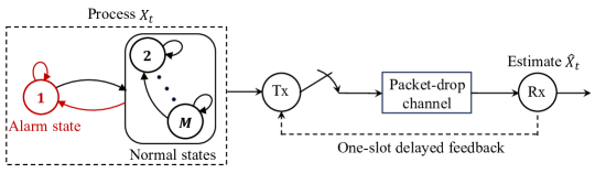
Figure 1: Remote estimation of a Markovian source with prioritized states.

This paper considers the remote estimation of a finite-state Markov chain $\{X_{t}\}_{t\geq 1}$ (see Fig. 1). The sensor observes the chain and decides when to send measurements to the receiver. The receiver is tasked with constructing the estimate process $\{\hat{X}_{t}\}_{t\geq 1}$ based on the received measurements. Each state, labeled as $1,2,\ldots,M$, can either represent a quantized level of a physical process or an abstract status of the system. Given that some states convey more important information than others, we utilize two semantic attributes to capture the data significance: the significance of estimation error and the cost of consecutive error. The first attribute is represented by the state-aware distortion (see [15, 16, 17, 18, 10]), where the cost of an estimation error depends not only on the physical discrepancy but also on the potential costs or risks incurred without a correct estimate of the state. The second attribute is motivated by the observation that successive reception of an estimation error may have a disastrous effect on the system, not mere accumulated costs during this period[19, 20, 17, 21]. We consider using a non-linear age function $g_{X_{t},\hat{X}_{t}}(\Delta_{t})$ to model the cost of being in estimation error $(X_{t},\hat{X}_{t})$ for $\Delta_{t}$ consecutive time slots up until time $t$. Recently, information aging has received significant attention in remote estimation systems. However, most existing studies have been devoted to linear age functions. The design of optimal transmission policies for optimizing significance-aware non-linear age metrics remains largely unexplored. Our main contributions are summarized below.

• We introduce a new metric, the significance-aware Age of Consecutive Error (AoCE), which accounts for both the significance of the current estimation error and the history-dependent cost of consecutive error. In essence, this metric assigns different costs and age functions to different estimation errors, offering the flexibility to handle the lasting impact of each error separately. For example, one might impose higher costs and exponential age functions on missed alarms while applying lower costs and logarithmic age functions to false alarms.

• The remote estimation problem is formulated as a countably infinite state Markov decision process (MDP) with unbounded costs. We give sufficient conditions on the source pattern, age functions, and channel reliability that yield a deterministic optimal policy for this MDP. We prove the optimal policy exhibits a switching structure. That is, the sensor triggers a transmission only when the age of the error $(X_{t},\hat{X}_{t})=(i,j)$ exceeds a fixed threshold $\tau^{*}_{i,j}$. We also give conditions under which the optimal policy degenerates into a simple threshold policy, i.e., featuring identical thresholds for all errors.

• Our switching policy is significant in several aspects. It circumvents the “curse of memory” and the “curse of dimensionality” of the MDP. One only needs to compute a small number of threshold values offline and store them in the sensor memory instead of solving a high-dimensional dynamic programming recursion and saving the results for infinitely many states. Moreover, it answers the fundamental question of “what and when to transmit”. According to [10], distortion-optimal policies only tell “whether to transmit when a certain error occurs”. That is, the optimal threshold for the error $(X_{t},\hat{X}_{t})=(i,j)$ is either $\tau^{*}_{i,j}=1$ (i.e., always transmit) or $\tau^{*}_{i,j}\rightarrow\infty$ (i.e., never transmit). By incorporating the error holding time as an additional dimension in the decision-making process, our approach further determines the optimal timing to initiate a transmission, allowing for transmissions to occur after several consecutive errors, i.e., $\tau_{i,j}^{*}\geq 1$.

• For numerical tractability, we propose a state-space truncation method and show the asymptotic optimality of the truncated MDP. We exploit these findings to develop a structured policy iteration (SPI) algorithm to compute the switching policy with reduced computation overhead. Our numerical results show that the optimal policy can be much better than the classic rule-, distortion-, and age-based policies. This highlights that the significance-aware AoCE offers more informed decisions and extends the current understanding of distortion and information aging.

The rest of this paper is organized as follows. In Section II, we discuss some related work. In Section III, we describe the system model and the formulation of the optimal transmission problem. In Section IV, we show the existence and structure of the optimal policy and the asymptotic optimality of the truncated MDP. We also present our structure-aware algorithm in this section. The numerical results and the conclusion are presented in Section V and Section VI.

II Related Work

In the remote estimation literature, the primary objective has been to minimize distortion over constraints on available resources, such as channel bandwidth or energy budget. Since distortion depends on the physical discrepancy between the original and reconstructed signals, optimal transmission and estimation policies must be signal-aware and derived by accounting for the source’s evolution pattern. Numerous studies have been devoted to linear Gaussian systems. Remote estimation of a scalar Gaussian source with communication costs was studied in[22], where the authors proved that a threshold transmission policy (i.e., the sensor transmits whenever the current error exceeds a threshold) and a Kalman-like estimator are jointly optimal. The results were further extended to systems with multidimensional Gaussian sources and energy-harvesting sensors[6], hard constraints on transmission frequency[8], unreliable channels with adaptive noise[23] and packet drops[24], to name a few.

Another line of research focuses on the use of smart sensors (e.g., with Kalman filters) to pre-estimate the source states and then sends the estimated states, rather than the raw measurements, to the receiver[5, 7, 25, 26, 27]. Besides tractability, this approach establishes a connection between distortion and the Age of Information (AoI). It has been shown that the error covariance is a monotonic non-decreasing function of AoI. Consequently, AoI serves as a sufficient statistic for decision-making, and the optimal policy initiates a transmission whenever the age exceeds a threshold. These results suggest that, in such systems, measurements are more valuable when they are fresh. However, this may not always be the case, as AoI ignores the source pattern and is, therefore, signal-agnostic. For instance, in the remote estimation of Winner and Ornstein-Uhlenbeck processes[9, 29], the estimation error achieved by the distortion-optimal policy can be much smaller than that of the age-optimal policy.

Remote estimation of discrete-state Markov chains has gained significant interest in recent years[24, 30, 31]. A salient feature of Markov processes is that they evolve in a probabilistic manner; consequently, the estimation error does not necessarily evolve monotonically with AoI. Another reason traditional distortion and AoI metrics become inefficient in Markovian systems is that the states often convey richer information beyond simple physical amplitudes [10, 21]. Such motivated, the concept of semantics-aware estimation and a series of content-aware metrics that go beyond information accuracy and freshness have been proposed[19, 15, 16, 17, 20, 10, 21]. State-aware distortion was first introduced in[15] to represent the significance of different estimation errors. Performance analysis and comparison of different policies were studied in[17, 16, 18, 10]. Structural results of the optimal policy in resource-constrained systems were provided in [10]. Various age metrics have been proposed to address the shortcomings of AoI. State-aware AoI[19] and the Uncertainty of Information (UoI)[32] reveal that the information quality depends on the source state (i.e., content) and evolves at different rates. The Version Age of Information (VAoI) tracks the number of content changes and is more relevant than AoI in Markovian systems[33, 34, 35]. The Age of Incorrect Information (AoII) is a signal-aware metric that counts only the time elapsed since the system was last synced[20, 36]. However, these age metrics treat all estimation errors equally, leading to inadequate transmissions in alarm states but excessive transmissions in normal states.

The closest study to this paper is our previous work in[21], where we examined the optimal transmission policy for optimizing significance-aware linear age metrics of a binary Markov chain. This paper generalizes[21] in the following aspects: i) In this paper, we introduce a new change-aware age metric, termed AoCE, that resets upon error variations, based on which we extend the results to a general finite-state Markov chain. ii) While [21] showed that an optimal policy always exists for linear age metrics, this does not hold for non-linear age functions. In this paper, we give sufficient conditions on the age functions, source pattern, and channel reliability so that an optimal policy exists to have bounded average costs. iii) The proofs in [21] relied on analytical expressions of the switching policy, which do not apply to multi-state sources and non-linear age metrics. We can generalize the theoretical results and greatly simplify the proofs by adopting new proof techniques. iv) In[21], the optimal policy was obtained by exhaustively searching for two optimal thresholds using analytical results. In contrast, this paper presents an SPI algorithm that exploits the structural properties to reduce computation overhead.

III System Model and Problem Formulation

III-A Remote Estimation Model

Consider the remote state estimation model shown in Fig. 1. The system comprises four main components: an information source, a local sensor (transmitter), a remotely placed estimator (receiver), and a wireless channel.

The stochastic process considered is a finite-state, homogeneous, discrete-time Markov chain (DTMC) $\{X_{t}\}_{t\geq 1}$ defined on the finite state space

$$\mathcal{X}=\{1,2,\ldots,M\}.$$ (1)

Here, state $1$ is labeled as the “alarm” state. We note that the results in this paper extend automatically to models with multiple alarm states. For later reference, we distinguish between the following types of estimation errors.

• Missed alarm (MA) errors occur when the receiver falsely announces a normal state while the source is actually in the alarm state, i.e., $X_{t}=1,\hat{X}_{t}\neq 1$. Timely detection of abnormalities is crucial for decision-making and system maintenance.

• False alarm (FA) errors refer to erroneously raising an alarm at the receiver when the source is in a normal state, i.e., $X_{t}\neq 1,\hat{X}_{t}=1$. Although less critical than MA errors, FA errors can lead to unnecessary expenditure on checking the system thus wasting resources.

• Other normal errors are considered indistinguishable and are not of primary interest.

Let $Q$ denote the state transition probability matrix, where

$$Q=(Q_{i,j},i,j\in\mathcal{X}),~{}Q_{i,j}=\textrm{Pr}\{X_{t+1}=j|X_{t}=i\}.$$ (2)

To avoid pathological cases, we assume $Q$ is irreducible. Let $\mathcal{X}_{\textrm{ap}}$ and $\mathcal{X}_{\textrm{p}}$ denote the sets of states with and without self-transitions, respectively, where

$$\mathcal{X}_{\textrm{ap}}=\{i\in\mathcal{X}:Q_{i,i}>0\},~{}\mathcal{X}_{\textrm{p}}=\mathcal{X}-\mathcal{X}_{\textrm{ap}}.$$ (3)

The chain is called aperiodic if $\mathcal{X}_{\textrm{ap}}\neq\emptyset$. Without otherwise stated, we assume $Q$ is aperiodic.

The sensor sequentially observes the source realization $X_{t}$ and decides at every decision epoch (i.e., the beginning of time slot $t$) whether or not to transmit a new measurement. Let $A_{t}\in\{0,1\}$ denote the decision variable, where $A_{t}=1$ means transmission while $A_{t}=0$ means no transmission. We consider an error-prone channel with i.i.d. packet drops. Let $H_{t}\in\{0,1\}$ denote the packet dropout process, which is an i.i.d. Bernoulli process satisfying

$$\textrm{Pr}\{H_{t}=1\}=p_{s},~{}\textrm{Pr}\{H_{t}=0\}=1-p_{s}=p_{f}.$$ (4)

Here, $H_{t}=1$ denotes that the packet will reach the destination by the end of time slot $t$ (i.e., the decision epoch $t+1$ in continuous time). In contrast, $H_{t}=0$ indicates deep fading channel conditions and a transmission failure.

Upon successful reception, the receiver updates its estimate using the newly received measurement, i.e., $\hat{X}_{t+1}=X_{t}$, and sends an acknowledgment (ACK) packet to the sensor. Otherwise, a negative ACK (NACK) is feedback, and the remote estimate remains unchanged, i.e., $\hat{X}_{t+1}=\hat{X}_{t}$. We assume that ACK/NACK packets are delivered instantaneously and error-free. Therefore, the sensor knows precisely the remote estimate $\hat{X}_{t}$ at every decision epoch. The information available at the sensor up to time $t$ is

$$I_{t}=(X_{1:t},\hat{X}_{1:t},A_{1:t-1}).$$ (5)

At decision epoch $t$, a decision $A_{t}$ is taken according to a transmission rule $\pi_{t}$, i.e.,

$$A_{t}=\pi_{t}(I_{t})=\pi_{t}(X_{1:t},\hat{X}_{1:t},A_{1:t-1}).$$ (6)

A transmission policy is a sequence of transmission rules, i.e., $\pi=(\pi_{1},\pi_{2},\ldots)$. We call a policy stationary if it employs the same rule at every decision epoch. A policy is deterministic if, given the history $I_{t}$, it selects an action with certainty, while a randomized policy specifies a probability distribution on the action space.

III-B Significance of Estimation Errors

In classical remote state estimation, whether a measurement is discarded or transmitted does not depend on the significance of the measurement. A widely used metric is Hamming distortion, given by

$$d(X_{t},\hat{X}_{t})=\mathds{1}\{X_{t}\neq\hat{X}_{t}\},$$ (7)

where $\mathds{1}\{\cdot\}$ is the indicator function.

Recall that in our problem, the alarm state (labeled as state $1$) is of greater interest. Intuitively, MA errors typically incur higher costs than other estimation errors. Therefore, we employ a state-aware distortion metric that assigns different costs to different estimation errors[15, 10], i.e.,

$$\bar{d}(X_{t},\hat{X}_{t})\triangleq\begin{cases}D_{i,j},&\textrm{if}~{}(X_{t},\hat{X}_{t})=(i,j),i\neq j,\\ 0,&\textrm{otherwise.}\end{cases}$$ (8)

where $D_{i,j},i\neq j$ are non-negative constants.

A notable shortcoming of distortion lies in its history-independence. Although the source evolution is Markovian, the value of information carried by the measurement depends on the history of all past observations and decisions. For instance, not only does the instantaneous estimation error matter but also how long the system has been trapped in this error, i.e., the cost of consecutive estimation errors (or lasting impact for short)[21].

Definition 1.

In this paper, we introduce a new age process, termed Age of Consecutive Error (AoCE), to capture this history-dependent attribute, defined as

$$\Delta_{t}\triangleq\begin{cases}\Delta_{t-1}+1,&\textrm{if}~{}X_{t}\neq\hat{X}_{t},(X_{t},\hat{X}_{t})=(X_{t-1},\hat{X}_{t-1}),\\ 1,&\textrm{if}~{}X_{t}\neq\hat{X}_{t},(X_{t},\hat{X}_{t})\neq(X_{t-1},\hat{X}_{t-1}),\\ 0,&\textrm{if}~{}X_{t}=\hat{X}_{t}.\end{cases}$$ (9)

A comparison of AoCE to typical distortion and age metrics is depicted in Fig. 2.

(a) Distortion

(b) State-aware distortion

(c) AoI

(d) AoII

(e) AoCE

(f) Significance-aware AoCE

Figure 2: Illustration of typical distortion and age metrics, where $D_{1,2}=\alpha,D_{3,1}=\beta,\beta<1<\alpha$. New measurements are received at $t_{0}$ and $t_{3}$; however, an estimation error occurs because the source changes its state. The system is automatically synced at $t_{5}$. Distortion metrics only consider the cost of the current estimation error. In contrast, age-based metrics take into account the history of past observations. The AoI depends only on the receiver process and ignores the source evolution. The AoII increases by $1$ whenever an estimation error occurs, while the AoCE resets upon error variations. The significance-aware AoCE assigns exponential age penalties to MA errors and logarithmic penalties to FA errors to represent their relative importance to system performance.

Remark 1.

We note that AoCE (9) is change-aware, as it resets upon error changes, whereas AoII is change-agnostic and increments by $1$ regardless of the error type. This feature allows us to reconstruct AoII from AoCE without additional information, but the reverse is not possible. Moreover, it offers the flexibility to handle the lasting impact of different estimation errors separately. However, age alone may not suffice, as it ignores the significance of the current estimation error. This gives incentives to significance-aware age processes.

Let $S_{t}$ denote the system state at decision epoch $t$, where

$$S_{t}=(X_{t},\hat{X}_{t},\Delta_{t}).$$ (10)

The significance-aware AoCE for estimation error $(X_{t},\hat{X}_{t})$ at decision epoch $t$ is defined as

$$c(S_{t})=c(I_{t})\triangleq\bar{d}(X_{t},\hat{X}_{t})\cdot g_{X_{t},\hat{X}_{t}}(\Delta_{t}),$$ (11)

where $(g_{i,j}(\cdot),i,j\in\mathcal{X})$ are non-negative, non-decreasing, and possibly unbounded age functions, $g_{i,j}(\delta)$ represents the cost of being in state $(i,j)$ for $\delta$ consecutive time slots. Given that a no lasting cost is paid in synced states and erroneous states with unit age, we impose $g_{i,j}(0)=g_{i,j}(1)=1,\forall i,j\in\mathcal{X}$.

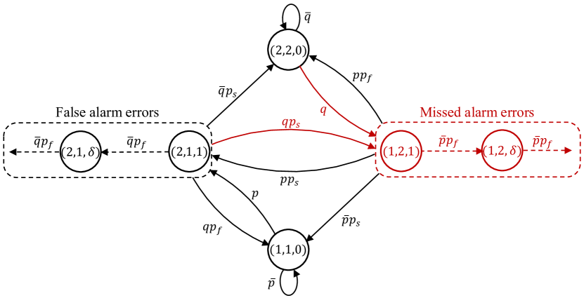
(a) $A_{t}=1$

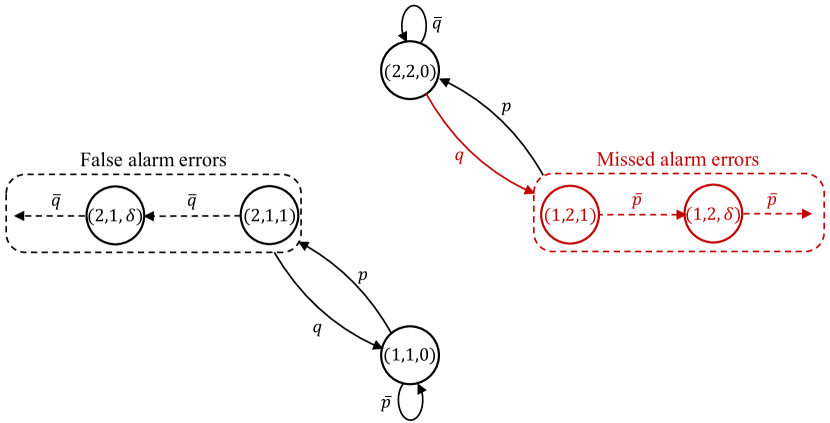
(b) $A_{t}=0$

Figure 3: DTMC representing the system state evolution of a two-state Markov source, where $p=Q_{1,2},q=Q_{2,1},\bar{p}=1-p,\bar{q}=1-q$.

Remark 2.

The significance of information is represented by the state-aware distortion $\bar{d}$, history-dependent lasting impact $\Delta_{t}$, and non-linear age functions $g_{i,j}$. The system state (10) can be interpreted as a collection of $M(M-1)$ dependent age processes, each corresponding to an estimation error (see Fig. 3). Notably, the AoCE (9) is not a sufficient statistic for decision-making unless Assumption 1 holds. We formally state this finding in Lemma 1. This result can be generalized to any age process whose evolution depends on the source pattern.

Assumption 1.

The source is non-prioritized, i.e., $D_{i,j}=D$ and $g_{i,j}=g$ for all $i\neq j$, and is symmetric with equal state change probabilities, i.e.,

$$Q_{i,j}=\begin{cases}p,&{\rm{if}}~{}i\neq j,\\ \bar{p},&{\rm{otherwise}}.\end{cases}$$ (12)

where $\bar{p}+(M-1)p=1,0<p<1$. In other words, the estimation errors contribute equally to the system in terms of both costs and occurrences.

Lemma 1.

The AoCE (9) is a sufficient statistic for the MDP only if Assumption 1 holds.

Proof.

Please see Appendix A. ∎

III-C System Evolution

The system state $\{S_{t}\}_{t\geq 1}$ is a three-dimensional controlled Markov chain. It is possible to achieve the desired performance by controlling the chain’s transition probabilities. Let

$$P=(P_{s,s^{\prime}}(a),s,s^{\prime}\in\mathcal{S},a\in\mathcal{A}),$$ (13)

denote the transition probability matrix, where

$$P_{s,s^{\prime}}(a)=\textrm{Pr}\{S_{t+1}=s^{\prime}|S_{t}=s,A_{t}=a\}$$ (14)

is the probability of transitioning to state $s^{\prime}$ at decision epoch $t+1$, given that the system is in state $s$ and the action $a$ is taken at decision epoch $t$.

Fig. 3 illustrates the system evolution of a two-state source. There are $2$ dependent age processes interconnected through the synced states. The always-transmission policy (i.e., $A_{t}=1,t\geq 1$) induces an irreducible Markov chain, whereas the non-transmission policy (i.e., $A_{t}=0,t\geq 1$) divides the state space into two isolated groups. The transition probabilities of a multi-state model are given as follows.

For any estimation error $(i,j),i\neq j$ with age $\delta\geq 1$, if the sensor decides not to transmit, the system will: (1) remain in this error, i.e., $s^{\prime}=(i,j,\delta+1)$, with probability (w.p.) $Q_{i,i}$, (2) become synced, i.e., $s^{\prime}=(j,j,0)$, w.p. $Q_{i,j}$, or (3) change to another error $(k,j,1),k\neq i/j$ w.p. $Q_{i,k}$. Thus, we have

$$\textrm{Pr}\{s^{\prime}|(i,j,\delta),0\}=\begin{cases}Q_{i,i},&\textrm{if}~{}s^{\prime}=(i,j,\delta+1),\\ Q_{i,j},&\textrm{if}~{}s^{\prime}=(j,j,0),\\ Q_{i,k},&\textrm{if}~{}s^{\prime}=(k,j,1),k\neq i/j,\\ 0,&\textrm{otherwise.}\end{cases}$$ (15)

If the sensor initiates a transmission, the measurement will be successfully decoded at the receiver w.p. $p_{s}$. In this case, the system will either enter a synced state $(i,i,0)$ w.p. $Q_{i,i}p_{s}$ or change to an error $(k_{1},i,1),k_{1}\neq i$ w.p. $Q_{i,k_{1}}p_{s}$. On the other hand, if the measurement is dropped out w.p. $p_{f}$, the system will: (1) stay in the current error w.p. $Q_{i,i}p_{f}$, (2) become synced w.p. $Q_{i,j}p_{f}$, or (3) change to another error $(k_{2},j,1),k_{2}\neq i/j$ w.p. $Q_{i,k_{2}}p_{f}$. We may write

$$\textrm{Pr}\{s^{\prime}|(i,j,\delta),1\}=\begin{cases}Q_{i,i}p_{s},&\textrm{if}~{}s^{\prime}=(i,i,0),\\ Q_{i,k_{1}}p_{s},&\textrm{if}~{}s^{\prime}=(k_{1},i,1),k_{1}\neq i,\\ Q_{i,i}p_{f},&\textrm{if}~{}s^{\prime}=(i,j,\delta+1),\\ Q_{i,j}p_{f},&\textrm{if}~{}s^{\prime}=(j,j,0),\\ Q_{i,k_{2}}p_{f},&\textrm{if}~{}s^{\prime}=(k_{2},j,1),k_{2}\neq i/j,\\ 0,&\textrm{otherwise.}\end{cases}$$ (16)

For any synced state $(i,i,0),\forall i\in\mathcal{X}$, the remote estimate will remain in state $i$ with certainty, regardless of whether a new measurement is received or not. Thus, the system will either remain synced w.p. $Q_{i,i}$, or enter an estimation error $(k,i,1),k\neq i$ w.p. $Q_{i,k}$. Formally, for each $a\in\{0,1\}$,

$$\textrm{Pr}\{s^{\prime}|(i,i,0),a\}=\begin{cases}Q_{i,i},&\textrm{if}~{}s^{\prime}=(i,i,0),\\ Q_{i,k},&\textrm{if}~{}s^{\prime}=(k,i,1),k\neq i,\\ 0,&\textrm{otherwise.}\end{cases}$$ (17)

It should be noted that, in all the above cases, the AoCE is no greater than $1$ if the source is in a state $i\in\mathcal{X}_{\textrm{p}}$.

Lemma 2.

The DTMC $\{S_{t}\}_{t\geq 1}$ controlled by the always-transmission policy is irreducible and positive recurrent. Moreover, for every pair of states $s$ and $s^{\prime}$ in $\mathcal{S}$, the expected first passage time from $s$ to $s^{\prime}$ is finite.

Proof.

Please see Appendix B. ∎

III-D Optimal Transmission Problem – MDP Formulation

The goal is to achieve a desired balance between estimation performance and communication cost. Given the cost of each transmission $\lambda$, the per-stage cost of taking an action $A_{t}$ in state $S_{t}$ is given by

$$l(S_{t},A_{t})=c(S_{t})+\lambda\mathds{1}\{A_{t}\neq 0\}.$$ (18)

The expected average cost of a transmission policy $\pi$ over an infinite horizon is defined as

$$\mathcal{L}(\pi)\triangleq\limsup_{T\rightarrow\infty}\frac{1}{T}\sum_{t=1}^{T}\mathbb{E}^{\pi}\bigl{[}l(S_{t},A_{t})\big{|}S_{1}=s_{1}\bigr{]},$$ (19)

where $\mathbb{E}^{\pi}$ represents the conditional expectation, given that policy $\pi$ is employed with initial state $s_{1}$. The sensor aims to determine the optimal policy $\pi^{*}$ to minimize (19), i.e.,

$$\mathcal{L}^{*}=\inf_{\pi\in\Pi}\mathcal{L}(\pi),$$ (20)

where $\Pi$ is the set of all admissible policies.

Problem (20) is a Markov Decision Process (MDP) with an average cost optimality criterion. More specifically, the MDP can be described by a 4-tuple $(\mathcal{S},\mathcal{A},P,l)$, where $\mathcal{S}$ is the state space of all possible values of $S_{t}$, $\mathcal{A}=\{0,1\}$ is the action space, $P$ is the transition probability matrix defined in (13), and $l$ is the cost function given by (18).

The state space $\mathcal{S}$ is a union of the set of synced states $\mathcal{S}_{0}$ and $M(M-1)$ sets of age of estimation errors, i.e., $\mathcal{S}_{i,j},\forall i\neq j$, where

$$\mathcal{S}_{0}\triangleq\{(i,i,0):i\in\mathcal{X}\},$$ (21)

$$\mathcal{S}_{i,j}\triangleq\begin{cases}\{(i,j,\delta):\delta\geq 1\},&\textrm{if}~{}i\neq j,i\in\mathcal{X}_{\textrm{ap}},\\ \{(i,j,1)\},&\textrm{if}~{}i\neq j,i\in\mathcal{X}_{\textrm{p}}.\end{cases}$$ (22)

We note that $\mathcal{S}$ is a countably infinite set because the ages corresponding to each estimation error can be unbounded. Hence, the problem encounters computing and memory challenges since classical value iteration methods cannot iterate over an infinite state space. Moreover, due to the unbounded per-stage costs, an optimal policy may not exist[39]. The following questions relating to the optimal policy are of interest.

• Under what conditions does an optimal policy exist?

• Are there any special structures of the optimal policy that facilitate policy implementation and computation?

• Is it possible to achieve asymptotic optimality by approximating the MDP with a finite state space?

• How to compute the optimal policy with reduced computation?

IV Main Results

This section aims to answer the above questions. We first give sufficient conditions on the source pattern, age functions, and channel reliability that yield a deterministic optimal policy for the MDP. Next, we prove that the optimal policy exhibits a switching structure, which facilitates policy storage and algorithm design. We also give sufficient conditions under which the optimal policy degenerates into a simple threshold policy. For numerical tractability, we propose a state-space truncation method and show the asymptotic optimality of the truncated MDP. By exploiting these findings, we develop a structure-aware algorithm to compute this switching policy with reduced computation overhead.

IV-A Existence of an Optimal Policy

Recall that the AoCE is countably infinite, and the age functions are non-decreasing and unbounded. Consequently, the long-term average cost may never be bounded, no matter how we choose the transmission policy. Thus, we will be concerned with the conditions under which an optimal policy exists to achieve bounded long-term costs.

Assumption 2 gives sufficient conditions, based on which we show the existence of an optimal policy in Theorem 1. This result reveals that the policy space $\Pi$ can be reduced to a small subset of Markovian (i.e., independent of $S_{1:t-1}$), stationary, and deterministic policies without losing optimality. Moreover, since the optimal policy depends only on the current observation, all previous measurements can be discarded, thereby saving sensor memory.

Assumption 2.

The age functions, source pattern, and channel condition satisfy the following convergence conditions

$$\lim_{\delta\rightarrow\infty}\frac{g_{i,j}(\delta+1)}{g_{i,j}(\delta)}<\frac{1}{Q_{i,i}p_{f}},~{}\forall i\in\mathcal{X}_{\rm{ap}},i\neq j,$$ (23)

where $Q_{i,i}p_{f}$ represents the probability of remaining in error $(i,j)$ after each transmission attempt.

Theorem 1.

Suppose Assumption 2 holds. Then there exists an optimal stationary deterministic policy $\pi^{*}$ such that for every $s\in\mathcal{S}$, $a=\pi^{*}(s)$ solves the following Bellman’s optimality equation

$$\mathcal{L}^{*}+h(s)=\min_{a}\{l(s,a)+\sum\nolimits_{s^{\prime}}P_{s,s^{\prime}}(a)h(s^{\prime})\},$$ (24)

where $h$ is a bounded function, $\mathcal{L}^{*}$ is the minimal average cost independent of the initial state $s_{1}$.

Proof.

Please see Appendix C. ∎

Remark 3.

The conditions in Assumption 2 are relatively relaxed if the source evolves rapidly and the channel condition is good, i.e., when $Q_{i,i}$ and $p_{f}$ are small. The intuition behind this is that frequent state changes in the source lead to more frequent error variations (age drops), and good channel conditions increase the likelihood of successful transmissions. Note that in the remote estimation of linear Gaussian processes, the system is easier to stabilize if the source evolves slowly[7, 26]. This notable contradiction arises because the error covariance of linear systems increases monotonically with time and only drops when a new measurement is received. From this perspective, the Markovian nature helps resist lasting impact.

Remark 4.

The convergence condition depends on the underlying source statistics and how we define the “age”. If the age is defined as the time elapsed since the last data reception, i.e., the AoI, then the convergence condition is

$$\lim_{\delta\rightarrow\infty}\frac{g(\delta+1)}{g(\delta)}<\frac{1}{p_{f}}.$$ (25)

We note that (25) is independent of the source statistics. This implies that AoI is inefficient for Markovian sources.

If the AoII is considered, the condition becomes

$$\lim_{\delta\rightarrow\infty}\frac{g(\delta+1)}{g(\delta)}<\frac{1}{1-\min_{i\neq j}\{Q_{i,j}p_{f}+Q_{i,i}p_{s}\}}.$$ (26)

Given that

$$\frac{1}{\max_{i}\{Q_{i,i}\}p_{f}}>\frac{1}{1-\min_{i\neq j}\{Q_{i,j}p_{f}+Q_{i,i}p_{s}\}}>\frac{1}{p_{f}},$$ (27)

it follows that the more information we utilize in defining the “age”, the more relaxed the restrictions on age functions will be.

As a result, we provide several age functions and derive their convergence conditions. It reveals that an optimal policy trivially exists when the age functions are bounded, linear, or logarithmic; it also holds for exponential functions with rate constraints. Similar analyses can be applied to other age metrics, e.g., [19, 20, 35, 21].

Corollary 1.

The assertion of Theorem 1 holds if

• $g_{i,j}(\delta)$ is an upper bounded clipping function, i.e.,

  $$g_{i,j}(\delta)=\begin{cases}g_{i,j}(\delta),&{\rm{if}}~{}\delta\leq\Delta_{\rm{max}},\\ g_{i,j}(\Delta_{\rm{max}}),&{\rm{otherwise.}}\end{cases}$$ (28)

  where $\Delta_{\rm{max}}$ is a finite constant.

• $g_{i,j}(\delta)=\alpha\delta+\beta$ is linear, where $\alpha\geq 0$.

• $g_{i,j}(\delta)=\log(\alpha\delta)+\beta$ is logarithmic, where $\alpha\geq 0$.

• $g_{i,j}(\delta)=\alpha^{\beta\delta}+\zeta$ is an exponential function, where the base and power satisfy $\alpha^{\beta}<1/(Q_{i,i}p_{f})$. For example, if $g_{i,j}(\delta)=e^{\beta\delta}+\zeta$, we impose $0\leq\beta<-\ln{(Q_{i,i}p_{f})}$; if $g_{i,j}(\delta)=\alpha^{\delta}+\zeta$, we impose $1\leq\alpha<1/(Q_{i,i}p_{f})$.

IV-B Structure of an Optimal Policy

Next, we show that the optimal policy has a switching structure. This result significantly remedies the “curse of memory” and the “curse of dimensionality.” Moreover, under Assumption 1, we show that the optimal policy degenerates into a threshold policy, i.e., featuring identical thresholds.

Theorem 2.

The optimal policy, if it exists, exhibits a switching structure. That is, for any given estimation error $(i,j)$ with age $\delta\geq 1$, the sensor initiates a transmission only when $\delta$ exceeds a certain threshold $\tau_{i,j}^{*}\geq 1$. Formally, we write

$$\pi^{*}(s)=\begin{cases}1,&{\rm{if}}~{}\delta\geq\tau_{i,j}^{*},i\neq j,\\ 0,&{\rm{otherwise.}}\end{cases}$$ (29)

where $\tau_{i,j}^{*}=1$ means always transmitting in estimation error $(i,j)$, whereas $\tau_{i,j}^{*}\rightarrow\infty$ means no transmission.

Proof.

Please see Appendix D. ∎

The condition that yields a threshold optimal policy is as follows.

Corollary 2.

Under Assumption 1, the optimal policy degenerates to a simple threshold policy, i.e., $\tau_{i,j}^{*}=\tau^{*},\forall i\neq j$.

Proof.

Please see Appendix E. ∎

Remark 5.

The nice property of the switching policy (29) is its simplicity in implementation and computation: i) to embed the optimal policy in the sensor memory, one only needs to store at most $M(M-1)$ estimation errors and their corresponding threshold values instead of all possible state-action pairs; ii) to implement the policy in a real-time sensor scheduler, trigger a transmission only when the age of the current estimation error exceeds the corresponding threshold and remain silent otherwise; iii) to compute the optimal policy, it suffices to search for a small number of optimal thresholds offline as opposed to solving a high-dimensional dynamic programming recursion offline.

Remark 6.

Theorem 2 answers the fundamental question of “what and when to transmit”. According to [10], distortion-optimal policies, both vanilla, and state-aware, specify a deterministic mapping from estimation error to transmission decision, guiding us on “whether to transmit when a certain error occurs”. By exploiting the lasting impact of the errors, our approach further determines the optimal timing (the threshold of error holding time) to initiate a transmission. Therefore, existing results on state-aware distortion (see[16, 10]) can be viewed as special cases where $\tau_{i,j}^{*}=1$. An important takeaway is that the more semantic attributes we utilize, the fewer transmissions are needed.

IV-C Problem Approximation and Asymptotic Optimality

We have shown several properties of the optimal policy. However, it is impossible to analytically calculate the switching policy for general source patterns and age functions because i) computing the stationary distribution $\mu^{\pi}$ of the infinite-state Markov chain induced by a switching policy $\pi$ is a non-trivial task; ii) the expected average cost, i.e., $\mathcal{L}(\pi)=\sum_{s\in\mathcal{S}}\mu^{\pi}(s)l(s,\pi(s))$, may not have closed-form expressions since the age functions are possibly non-linear; iii) even with such results at hand, $\mathcal{L}(\pi)$ is a high dimensional, non-convex function, which does not translate into analytical expressions for the optimal thresholds[21].

Thus, we need to resort to numerical methods, either policy iteration or value iteration, to compute the optimal policy. Although Theorem 2 considerably reduces the policy searching space, finding the optimal thresholds is still challenging as we cannot iterate over infinitely many states.

To make the problem numerically tractable, we truncate the state space and propose a finite-state approximate MDP. The truncated AoCE is defined as

$$\Delta_{t}(N)\triangleq\min\{\Delta_{t},N\},$$ (30)

where $\Delta_{t}$ is the original age process defined in (9), $N>0$ is the truncation size. In this way, the age associated with each estimation error $(i,j)$ is confined within

$$\mathcal{S}_{i,j}^{N}=\begin{cases}\{(i,j,\delta):1\leq\delta\leq N\},&\textrm{if}~{}i\neq j,i\in\mathcal{X}_{\textrm{ap}},\\ \{(i,j,1)\},&\textrm{if}~{}i\neq j,i\in\mathcal{X}_{\textrm{p}}.\\ \end{cases}$$ (31)

and the truncated state space is given by

$$\mathcal{S}^{N}=\mathcal{S}_{0}\bigcup_{i\neq j}\mathcal{S}^{N}_{i,j}.$$ (32)

The state space truncation, however, inevitably changes the stationary distribution of the induced Markov chain, yielding inconsistent system performance. Consequently, an optimal policy for the truncated MDP may be suboptimal for the original problem. Generally, there is no guarantee that the truncated MDP will converge to the original one as $N$ approaches infinity[39]. Thus, we will be concerned with the performance loss caused by state space truncation. Fortunately, the following result establishes the asymptotic optimality of the truncated MDP, and we shall feel safe to truncate the AoCE with an appropriately chosen $N$.

Theorem 3.

Suppose Assumption 2 holds. Let $\mathcal{L}^{*}(N)$ denote the minimal cost of the truncated MDP. Then, $\mathcal{L}^{*}(N)$ converges to the optimal value $\mathcal{L}^{*}$, i.e., $\lim_{N\rightarrow\infty}\mathcal{L}^{*}(N)\rightarrow\mathcal{L}^{*}$, at an exponential rate of $\max_{i\in\mathcal{X}_{\rm{ap}}}\{(Q_{i,i}p_{f})^{N}\}$.

Proof.

Please see Appendix F. ∎

IV-D Structured Policy Iteration Algorithm

Classical unstructured policy and value iteration methods can be applied to solve Bellman’s equation (24) and obtain an optimal stationary deterministic policy[40]. Let $\Pi^{\textrm{SD}}$ denote the space of stationary deterministic policies, and $\Pi^{*}$ denote the space of monotonically non-decreasing policies, where $\Pi^{*}\subset\Pi^{\textrm{SD}}$. Let us assume there are $m$ ($m\leq M(M-1)$) infinite-state age processes, each with a truncation size of $N$ ($m\ll N$). Recall that there are $|\mathcal{S}^{N}|=M^{2}-m+mN$ states in the truncated state-space and $|\mathcal{A}|=2$ actions. Then, the numbers of possible policies in $\Pi^{*}$ and $\Pi^{\textrm{SD}}$ are given by

$$|\Pi^{*}|=N^{m},~{}|\Pi^{\textrm{SD}}|=|\mathcal{A}|^{|\mathcal{S}^{N}|}=2^{M^{2}-m+mN}\approx 2^{mN}.$$ (33)

Taking a logarithm of these numbers yields

$$\log_{2}(|\Pi^{*}|)=m\log_{2}(N)\ll\log_{2}(|\Pi^{\textrm{SD}}|)=mN.$$ (34)

Therefore, the reduction in the size of the structured policy space is quite significant compared to the set of all deterministic policies. Moreover, unstructured iteration methods evaluate all possible policies in a stochastic manner, which makes the convergence rate even slower.

Next, we propose a structured policy iteration (SPI) algorithm that exploits the structure results established in Theorem 2. The algorithm proceeds as follows.

• Initialization: Arbitrarily select initial policy $\pi^{k}$, reference state $s_{\textrm{ref}}$, and set $k=0$; Choose a truncation size $N$ such that $(Q_{i,i}p_{f})^{N}<\epsilon$ for all $i\in\mathcal{X}_{\textrm{ap}}$, where $\epsilon$ is an arbitrarily small constant.

• Policy Evaluation Step: Find a scalar $\mathcal{L}^{k}$ and a vector $h^{k}$ by solving

  $$\mathcal{L}^{k}+h^{k}(s)=l(s,\pi^{k}(s))+\sum_{s^{\prime}\in\mathcal{S}^{N}}P_{s,s^{\prime}}(\pi^{k}(s))h^{k}(s^{\prime})$$ (35)

  for all $s\in\mathcal{S}^{N}$ such that $h^{k}(s_{\textrm{ref}})=0$.

• Policy Improvement Step: Find $\pi^{k+1}$ that satisfies for all $s\in\mathcal{S}^{N}$

  $$l(s,\pi^{k+1}(s))+\sum_{s^{\prime}\in\mathcal{S}^{N}}P_{s,s^{\prime}}(\pi^{k+1}(s))h^{k}(s^{\prime})=\min_{a\in\mathcal{A}}\bigg{[}l(s,a)+\sum_{s^{\prime}\in\mathcal{S}^{N}}P_{s,s^{\prime}}(a)h^{k}(s^{\prime})\bigg{]}.$$ (36)

  To ensure the known policy structure, $\pi^{k+1}(s)$ is calculated in the increasing order of the AoCE. If an optimal action $a^{*}=\pi^{k}(s)$ for state $s=(i,j,\delta)$ is to initiate a transmission, then the optimal action for the remaining states $(i,j,\delta^{\prime}),\delta^{\prime}>\delta$ is to transmit without further computation. This implies that the complexity of a structured policy search is independent of the boundary size $N$ and depends only on the switching curve. Therefore, the actual complexity of SPI is $\prod_{i\neq j}\tau_{i,j}^{*}\ll N^{m}$.

• Stopping Criterion: If $\pi^{k+1}=\pi^{k}$, the algorithm terminates with $\mathcal{L}^{*}=\mathcal{L}^{k}$ and $\pi^{*}=\pi^{k}$; otherwise increase $k=k+1$ and return to step 2.

V Numerical Results

In this section, we provide numerical simulations to illustrate our results on the optimal switching policy.

In the first example, we show the impact of significance-aware non-linear aging on the switching curve. To isolate the effect of other factors on the policy, we consider a symmetric source of the form in (12) with the following parameters: $M=4,p=0.1,\bar{p}=0.7$, and $D_{i,j}=1,\forall i\neq j$. We assign exponential age functions to MA errors and logarithmic age functions to FA errors, i.e.,

$$g_{i,j}(\delta)=\begin{cases}e^{0.3\delta},&\textrm{if}~{}i=1,j\neq 1,\\ \log(\delta)+1,&\textrm{if}~{}i\neq 1,j=1,\\ 1,&\textrm{otherwise.}\end{cases}$$ (37)

The parameters in (23) can be computed as

$$\lim_{\delta\rightarrow\infty}\frac{g_{i,j}(\delta+1)}{g_{i,j}(\delta)}=\begin{cases}e^{0.3},&\textrm{if}~{}i=1,j\neq 1,\\ 1,&\textrm{otherwise.}\end{cases}$$ (38)

which satisfies the convergence condition. By Theorem 2, there exists a switching optimal policy.

The optimal thresholds for different communication cost $\lambda$ with a fixed success probability $p_{s}$ are shown in Table I. Similarly, the thresholds for different $p_{s}$ with a fixed $\lambda$ are presented in Table II. Herein, $(*)$ represents the distortion-optimal policy. We observe that for both policies, the thresholds are non-decreasing in $\lambda$ for fixed $p_{s}$ and are non-increasing in $p_{s}$ for fixed $\lambda$. When communication is costly, or the channel condition is relatively bad, the optimal policy is to transmit less frequently (or never transmit) in FA and normal errors while consistently prioritizing MA errors. In contrast, the distortion-optimal policy either initiates a transmission in all errors (i.e., $\tau_{i,j}=1,\forall i\neq j$) when the communication is inexpensive ($\lambda\leq 1$), or remains silent otherwise (i.e., $\tau_{i,j}=\infty,\forall i\neq j$). This highlights the effectiveness of exploiting data significance in such systems.

TABLE I: Numerical results with different communication costs $\lambda$ for $p_{s}=0.9,N=20$.

$\lambda$	Optimal thresholds				Average cost
	MA errors	FA errors	Normal errors	$*$	Ours	$*$
0	1	1	1	1	0.35	0.35
1	1	1	1	1	0.67	0.67
2	1	1	$\infty$	$\infty$	0.88	1.63
3	2	3	$\infty$	$\infty$	0.99	1.63
4	3	11	$\infty$	$\infty$	1.04	1.63
5	3	$\infty$	$\infty$	$\infty$	1.05	1.63

TABLE II: Numerical results with different channel conditions $p_{s}$ for $\lambda=2,N=20$.

$p_{s}$	Optimal thresholds				Average cost
	MA errors	FA errors	Normal errors	$*$	Ours	$*$
0.4	2	$\infty$	$\infty$	$\infty$	1.05	1.63
0.5	2	8	$\infty$	$\infty$	1.04	1.63
0.6	2	3	$\infty$	$\infty$	0.99	1.63
0.7	2	2	$\infty$	$\infty$	0.96	1.63
0.8	1	2	$\infty$	$\infty$	0.92	1.63
0.9	1	1	$\infty$	$\infty$	0.88	1.63
1.0	1	1	$\infty$	$\infty$	0.85	1.63

TABLE III: Performance comparisons with different policies for $p_{s}=0.9,N=20$.

$\lambda$	Achievable minimal average costs
	Randomized	Periodic	distortion	AoI	AoII	Threshold	Ours
0	0.31	0.31	0.31	0.31	0.31	0.31	0.31
1	0.93	0.85	0.59	0.84	0.62	0.62	0.59
2	1.46	1.05	1.32	1.14	0.91	0.88	0.73
3	1.20	1.20	1.34	1.42	1.14	0.97	0.80
4	1.20	1.20	1.34	1.65	1.34	1.01	0.85
5	1.20	1.20	1.34	1.84	1.34	1.04	0.88

We continue to consider a general asymmetric source with

$$Q=\begin{bmatrix}0.7&0.1&0.1&0.1\\ 0.05&0.7&0.15&0.1\\ 0.1&0.1&0.6&0.2\\ 0.05&0.1&0.05&0.8\end{bmatrix}.$$ (39)

The other parameters are the same as in the first example. For comparison purposes, we consider several benchmark policies: i) Randomized policy, which transmits at every slot with a fixed probability $p_{\alpha}\in[0,1]$; ii) periodic policy, which transmits packets every $d\geq 1$ slots; iii-iv) AoI/AoII policy, which attains an optimal trade-off between (linear) AoI/AoII minimization and communication utilization; v) threshold policy, which initiates a transmission whenever the AoCE exceeds a threshold $\delta_{\textrm{th}}\geq 1$ independent of the error. We numerically search for the optimal values $p_{\alpha}^{*},d^{*},\delta^{*}_{\textrm{th}}$, as well as the optimal thresholds $\tau_{i,j}^{*}$ for the distortion, AoI/AoII, and switching policies. The performance of these policies is summarized in Table III. We categorize these policies into rule-based (e.g., randomized and periodic) and age-based (e.g., AoI- and AoII-optimal).

It is observed that when communication is cost-free ($\lambda=0$), all the policies employ the always-transmission strategy. The distortion and switching policies achieve optimal performance when communication is inexpensive ($\lambda\leq 1$). In contrast, when communication is expensive ($\lambda\geq 3$), the optimal randomized and periodic policies adopt the non-transmission strategy, resulting in significant lasting costs. An interesting observation is that the distortion- and AoII-optimal policies perform poorly compared to the others when $\lambda\geq 3$. This occurs because they transmit measurements in less important errors, leading to poor estimation performance and unnecessary transmission costs. The AoI metric, however, shows obvious disadvantages in our problem since it completely ignores the source evolution and sends information even when the system is in synced states. The reason accounting for the performance losses of the distortion and threshold policies is that make decisions based on insufficient statistics. Specifically, the distortion policy relies on $(X_{t},\hat{X_{t}})$, while the threshold policy utilizes only the AoCE $\Delta_{t}$.

Next, we examine the behavior of the switching policy. The optimal thresholds for $\lambda=3$ are given by

$$[\tau^{*}_{i,j}]_{4\times 4}=\begin{bmatrix}\infty&2&2&3\\ 3&\infty&\infty&\infty\\ \infty&\infty&\infty&\infty\\ 1&1&1&\infty\end{bmatrix}.$$ (40)

An important observation is that the switching curve depends on the source pattern. The thresholds for MA errors (i.e., the first row in (40)) are larger than those in the last row. This can be attributed to the high probability of the source remaining in state $4$ across consecutive time slots. In other words, the system will likely remain in this error for an extended period if no measurement is received. Therefore, it is worth transmitting measurements in this error, even though the age penalties are relatively small. In outline, our approach determines the optimal timing for data transmission, offering more informed decisions and extending the current understanding of distortion and information aging.

VI Conclusion

In this paper, we have investigated the semantics-aware remote estimation of an asymmetric Markov chain through the significance-aware AoCE. We first give sufficient conditions for the existence of an optimal policy. We prove that a switching policy is optimal and developed a structure-aware algorithm to find the optimal thresholds with reduced computation. Our numerical comparisons show that the optimal policy can be much better than existing rule-, distortion- and age-based policies. The results in this paper generalize recent research on distortion and information aging.

Appendix A Proof of Lemma 1

According to [38], the AoCE $\Delta_{t}$ is a sufficient statistic if it satisfies

• the controlled Markov property

  $$\textrm{Pr}\{\Delta_{t+1}|I_{t},A_{t}\}=\textrm{Pr}\{\Delta_{t+1}|\Delta_{t},A_{t}\},$$ (41)

• and the absorbing property

  $$\textrm{Pr}\{c(I_{t})|I_{t},A_{t}\}=\textrm{Pr}\{c(\Delta_{t})|\Delta_{t},A_{t}\}.$$ (42)

By (9), it is clear that the evolution of AoCE is dependent on the source pattern and transmission decision. Therefore, knowing the current age $\Delta_{t}$ is inadequate in inferring the next age $\Delta_{t+1}$. When the source transition matrix is of the special form given in (12), the state change probabilities are independent of the current state $X_{t}$ and the target state $X_{t+1}$. Hence, it makes no difference which error the system encounters. It suffices to know whether the system is erroneous or not and how long it has been in this error. According to (15)-(17), the transition probabilities of $\Delta_{t}$ are given by

$$\textrm{Pr}\{\delta^{\prime}|\delta,0\} =\begin{cases}\bar{p},&\textrm{if}~{}\delta=0,\delta^{\prime}=0,\\ 1-\bar{p},&\textrm{if}~{}\delta=0,\delta^{\prime}=1,\\ p,&\textrm{if}~{}\delta>0,\delta^{\prime}=0,\\ \bar{p},&\textrm{if}~{}\delta>0,\delta^{\prime}=\delta+1,\\ 1-p-\bar{p},&\textrm{if}~{}\delta>0,\delta^{\prime}=1.\end{cases}$$ (43)

$$\textrm{Pr}\{\delta^{\prime}|\delta,1\} =\begin{cases}\bar{p},&\textrm{if}~{}\delta=0,\delta^{\prime}=0,\\ 1-\bar{p},&\textrm{if}~{}\delta=0,\delta^{\prime}=1,\\ \bar{p}p_{s}+pp_{f},&\textrm{if}~{}\delta>0,\delta^{\prime}=0,\\ \bar{p}p_{f},&\textrm{if}~{}\delta>0,\delta^{\prime}=\delta+1,\\ 1-\bar{p}-pp_{f},&\textrm{if}~{}\delta>0,\delta^{\prime}=1.\end{cases}$$ (44)

Therefore, the Markov property is verified. The absorbing property is trivial as the one-stage cost is state-agnostic and depends only on the age $\Delta_{t}$. This completes the proof.

Appendix B Proof of Lemma 2

It is equivalent to show that the subsystem $Z_{t}=(X_{t},\hat{X}_{t})$ controlled by the always-transmission policy is positive recurrent. The transition probability matrix under the always-transmission policy is given by

$$R=(R_{z,z^{\prime}},z,z^{\prime}\in\mathcal{Z}),$$ (45)

where $\mathcal{Z}=\mathcal{X}\times\mathcal{X}$ and

$$R_{z,z^{\prime}} =\textrm{Pr}\{Z_{t+1}=z^{\prime}|Z_{t}=z,A_{t}=1\}$$

$$=\begin{cases}Q_{i,k}p_{s},&\textrm{if}~{}z=(i,j),z^{\prime}=(k,i),\\ Q_{i,k}p_{f},&\textrm{if}~{}z=(i,j),z^{\prime}=(k,j),\\ Q_{i,k},&\textrm{if}~{}z=(i,i),z^{\prime}=(k,i),\\ 0,&\textrm{otherwise.}\end{cases}$$ (46)

Since $Z_{t}$ is a finite-state Markov chain, the positive recurrence is verified if $R$ is irreducible[41], that is, every pair of states $(z,z^{\prime})$ communicates with each other. Let $z=(i,j),z^{\prime}=(m,n)$ be two distinct states in $\mathcal{Z}$. Since $Q$ is irreducible, the source can jump from state $i$ to state $n$ with a positive probability. Suppose this transition takes $t_{1}$ steps, and all transmission attempts fail. Thus, we have

$$\textrm{Pr}\{(i,j)\rightarrow(n,j)\}=Q_{i,n}^{t_{1}}(p_{f})^{t_{1}}>0.$$ (47)

We assume in the subsequent time slot, a new measurement is received w.p. $p_{s}$ and the estimate becomes $n$. After that, the source moves from state $n$ to state $m$ in $t_{2}$ steps, assuming all transmission attempts are unsuccessful. This implies

$$\textrm{Pr}\{(n,j)\rightarrow(m,n)\}=Q_{n,m}^{t_{2}+1}(p_{f})^{t_{2}}p_{s}>0.$$ (48)

Thus, the probability of transitioning from state $z$ to $z^{\prime}$ is

$$\textrm{Pr}\{z\rightarrow z^{\prime}\}=Q_{i,n}^{t_{1}}Q_{n,m}^{t_{2}+1}(p_{f})^{t_{1}+t_{2}}p_{s}>0.$$ (49)

Similarly, we can show that $\textrm{Pr}\{z\leftarrow z^{\prime}\}$ is also positive. Therefore, the chain $Z_{t}$ under the always-transmission policy is irreducible and positive recurrent. The positive recurrence implies that, for every state $z$ and $z^{\prime}$ in $\mathcal{X}\times\mathcal{X}$, the expected first passage time from $z$ to $z^{\prime}$ is finite.

Appendix C Proof of Theorem 1

The sufficient conditions that guarantee the existence of an optimal policy for the average-cost MDP with a countably infinite state space are presented in[39, Corollary 7.5.10]. We need to verify the following conditions: (C1) Given any positive constant $U$, the set $\mathcal{S}_{U}\triangleq\{s\in\mathcal{S}:l(s,a)\leq U~{}\textrm{for some}~{}a\}$ is finite. (C2) There exists a distinguished state $z\in\mathcal{S}$ and a $z$-standard policy. By (18), C1 can be verified via the non-transmission policy.

Definition 2.

A stationary policy is called standard if the underlying system induced by the policy forms an irreducible and positive recurrent Markov chain. Further, if there exists a state $z$ such that the expected first passage time and the expected first passage cost from any state $s$ to $z$ are finite, the policy is called $z$-standard.

To verify C2, let $\pi$ be the always-transmission policy. By Lemma 2, there exists a state $z\in\mathcal{S}$, say $z=(0,0,0)$, such that $\pi$ is $z$-standard and the expected first passage time from any state $s$ to $z$ is finite. It remains to show that the expected first passage cost is also finite. The system may remain in some estimation error for a period or jump between them alternately before reaching state $z$. Therefore, we need to ensure that the expected first passage cost incurred in each estimation error $(i,j)$ is finite. To establish this, we first define a fictitious “zero” state that will find applications in many places.

Definition 3.

For each estimation error $(i,j),i\in\mathcal{X}_{\rm{ap}},i\neq j$, we define a fictitious “zero” state that consists of all the synced states and other estimation errors with unit age, i.e.,

$$(i,j,0)\triangleq\mathcal{S}_{0}\cup\{(m,n,1):\forall m\neq n,(m,n)\neq(i,j)\}.$$ (50)

Let

$$\bar{\mathcal{S}}_{i,j}=\mathcal{S}_{i,j}\cup\{(i,j,0)\}$$ (51)

denote the extended subspace corresponding to error $(i,j)$.

Assume that the system will stay in error $(i,j)$ for $n$ consecutive time slots before moving to the “zero” state. The first passage cost along this sample path is given by

$$M_{i,j}(n)=\sum_{t=0}^{n}\big{(}D_{i,j}g_{i,j}(\delta+t)+\lambda\big{)}+\tilde{D},$$ (52)

where $\tilde{D}$ is the cost incurred in the “zero” state. Since $\tilde{D}$ is a finite constant, we omit it for brevity.

The probability that the system will stay in this error for $n$ consecutive time slots is

$$p_{i,j}(n)=(1-Q_{i,i}p_{f})(Q_{i,i}p_{f})^{n}.$$ (53)

Hence, the expected first passage cost is given by

$$\bar{M}_{i,j} =\sum_{n=0}^{\infty}p_{i,j}(n)M_{i,j}(n)$$

$$=\sum_{n=0}^{\infty}(1-Q_{i,i}p_{f})(Q_{i,i}p_{f})^{n}\big{(}D_{i,j}g_{i,j}(\delta+n)+\lambda\big{)}$$

$$=\lambda+(1-Q_{i,i}p_{f})D_{i,j}\sum_{n=0}^{\infty}\xi(n),$$ (54)

where $\xi_{i,j}(n)=(Q_{i,i}p_{f})^{n}g_{i,j}(\delta+n)$.

The proof is therefore reduced to showing that the summation $\sum_{n=0}^{\infty}\xi_{i,j}(n)$ is finite. By ratio test, the series $\{\xi_{i,j}(n)\}_{n\geq 0}$ converges if

$$\lim_{n\rightarrow\infty}\frac{\xi_{i,j}(n+1)}{\xi_{i,j}(n)}<1.$$ (55)

Rearranging the terms yields

$$\lim_{n\rightarrow\infty}\frac{g_{i,j}(\delta+n+1)}{g_{i,j}(\delta+n)}=\lim_{n^{\prime}\rightarrow\infty}\frac{g_{i,j}(n^{\prime}+1)}{g_{i,j}(n^{\prime})}<\frac{1}{Q_{i,i}p_{f}}.$$ (56)

This completes the proof.

Appendix D Proof of Theorem 2

By (17), transmitting in the synced states has no effect on the estimation performance but incurs additional communication costs. Thus, we have

$$\pi^{*}(s)=0,~{}\textrm{if}~{}i=j.$$ (57)

Then, we are only interested in the cases when $i\neq j$, or equivalently, $\delta\geq 1$. It is equivalent to show that the optimal policy is monotonically non-decreasing in $\delta$ for fixed $(i,j)$. We prove the monotonicity by showing that the following conditions hold[40, Theorem 8.11.3].

• (monotonicity) $l(s,a)$ is non-decreasing in $s$ for all $a$; $q(k|s,a)\triangleq\sum_{j=k}^{\infty}\textrm{Pr}\{j|s,a\}$ is non-decreasing in $s$ for all $k\in\mathcal{S}$ and $a\in\mathcal{A}$;

• (subadditivity) $l(s,a)$ is a subadditive function on $\mathcal{S}\times\mathcal{A}$; $q(k|s,a)$ is a subadditive function on $\mathcal{S}\times\mathcal{A}$ for all $k\in\mathcal{S}$.

To verify these conditions, we first give the following necessary definitions.

Definition 4.

For each error $(i,j),i\in\mathcal{X}_{\rm{ap}},i\neq j$, the states in the corresponding extended subspace $\bar{\mathcal{S}}_{i,j}$ are ordered by their age $\delta$. That is, for any two states $s_{-}$ and $s_{+}$ in $\bar{\mathcal{S}}_{i,j}$, we define $s_{-}\leq s_{+}$ if $\delta_{-}\leq\delta_{+}$.

Definition 5.

A multivariable function $f(x,y)$ is subadditive on $(x,y)$ if, for all $x_{-}\leq x_{+}$ and $y_{-}\leq y_{+}$, it holds that[40]

$$f(x_{+},y_{+})+f(x_{-},y_{-})\leq f(x_{+},y_{-})+f(x_{-},y_{+}).$$ (58)

We now establish the monotonicity of $l(s,a)$ and $q(k|s,a)$. Since $g_{i,j}$ is a monotone and non-decreasing function of $\delta$, the cost function

$$l(s,a)=D_{i,j}g_{i,j}(\delta)+\lambda a$$ (59)

is also monotonically non-decreasing. For each $a\in\{0,1\}$, the system will either stay in this error, i.e., $s^{\prime}=(i,j,\delta+1)$, or jump to the fictitious “zero” state (see Definition 3). The quantity $q(k|s,a)$ is given by

$$q(k|s,a=1) =\begin{cases}1,&\textrm{if}~{}k\leq(i,j,0),\\ Q_{i,i}p_{f},&\textrm{if}~{}(i,j,0)<k\leq(i,j,\delta+1),\\ 0,&\textrm{if}~{}k>(i,j,\delta+1).\end{cases}$$ (60)

$$q(k|s,a=0) =\begin{cases}1,&\textrm{if}~{}k\leq(i,j,0),\\ Q_{i,i},&\textrm{if}~{}(i,j,0)<k\leq(i,j,\delta+1),\\ 0,&\textrm{if}~{}k>(i,j,\delta+1).\end{cases}$$ (61)

Since $q(k|s,a)$ is a constant function for any given $a$ and $k$, the monotonicity condition follows.

Then, we verify the subadditivity of the functions $l(s,a)$ and $q(k|s,a)$. According to (59), the subadditivity of $l(s,a)$ is immediate. Let $s_{-}=(i,j,\delta_{-}),s_{+}=(i,j,\delta_{+}),a_{-}=0,a_{+}=1$. Then, we have

$$q(k| s_{+},a_{+})+q(k|s_{-},a_{-})=\begin{cases}2,&\textrm{if}~{}k\leq(i,j,0),\\ Q_{i,i}(1+p_{f}),&\textrm{if}~{}(i,j,0)<k\leq(i,j,\delta_{-}),\\ Q_{i,i}p_{f},&\textrm{if}~{}(i,j,\delta_{-})<k\leq(i,j,\delta_{+}),\\ 0,&\textrm{if}~{}k>(i,j,\delta_{+}).\end{cases}$$ (62)

$$q(k| s_{+},a_{-})+q(k|s_{-},a_{+})=\begin{cases}2,&\textrm{if}~{}k\leq(i,j,0),\\ Q_{i,i}(1+p_{f}),&\textrm{if}~{}(i,j,0)<k\leq(i,j,\delta_{-}),\\ Q_{i,i},&\textrm{if}~{}(i,j,\delta_{-})<k\leq(i,j,\delta_{+}),\\ 0,&\textrm{if}~{}k>(i,j,\delta_{+}).\end{cases}$$ (63)

It follows that

$$q(k|s_{+},a_{+})+q(k|s_{-},a_{-})\leq q(k|s_{+},a_{-})+q(k|s_{-},a_{+}).$$ (64)

Hence, $q(k|s,a)$ is a subadditive function.

Therefore, for any given estimation error $s=(i,j,\delta),i\neq j$, the optimal policy is monotonically non-decreasing in $\delta$,

$$\pi^{*}(s)=\begin{cases}1,&~{}\textrm{if}~{}\delta\geq\tau_{i,j}^{*},i\neq j,\\ 0,&~{}\textrm{if}~{}1\leq\delta<\tau_{i,j}^{*},i\neq j,\\ \end{cases}$$ (65)

where $\tau_{i,j}^{*}\geq 1$ is the threshold value corresponding to error $(i,j)$. Combing (57) and (65) gives

$$\pi^{*}(s)=\begin{cases}1,&~{}\textrm{if}~{}\delta\geq\tau_{i,j}^{*},i\neq j,\\ 0,&~{}\textrm{otherwise}.\\ \end{cases}$$ (66)

Therefore, the proof is complete.

Appendix E Proof of Corollary 2

By Lemma 1, if Assumption 1 holds, then the age process $\Delta_{t}$ is a sufficient statistic. Therefore, we only need to show that the optimal policy to the MDP with system state $\Delta_{t}$ and transition probabilities (43)-(44) is a threshold policy.

Similar to Theorem 2, the proof is reduced to proving that the optimal policy is monotonically non-decreasing in $\delta$. Thus, we need to verify the monotonicity and subadditivity of the functions $l(\delta,a)=Dg(\delta)+\lambda a$ and $q(k|\delta,a)\triangleq\sum_{j=k}^{\infty}\textrm{Pr}\{j|\delta,a\}$. Clearly, the conditions trivially hold for the cost function. The quantity $q(k|\delta,a)$ can be given by

$$q(k|\delta,0) =\begin{cases}1,&\textrm{if}~{}k\leq 0,\\ 1-\bar{p}-p,&\textrm{if}~{}0<k\leq 1,\\ \bar{p},&\textrm{if}~{}1<k\leq\delta+1,\\ 0,&\textrm{if}~{}k>\delta+1.\end{cases}$$ (67)

$$q(k|\delta,1) =\begin{cases}1,&\textrm{if}~{}k\leq 0,\\ 1-\bar{p}-pp_{f},&\textrm{if}~{}0<k\leq 1,\\ \bar{p}p_{f},&\textrm{if}~{}1<k\leq\delta+1,\\ 0,&\textrm{if}~{}k>\delta+1.\end{cases}$$ (68)

where $p$ and $\bar{p}$ are defined in (12). One can easily show that $q(k|\delta,a)$ is monotone and subadditive. Therefore, under Assumption 1, the optimal policy is a threshold policy. In other words, the optimal switching policy given in Theorem 2 has identical thresholds.

Appendix F Proof of Theorem 3

We prove the result in the following two steps.

• For any given switching policy, show that the cost of the truncated problem converges to the original one as $N\rightarrow\infty$, i.e., $\lim_{N\rightarrow\infty}\mathcal{L}(\pi,N)\rightarrow\mathcal{L}(\pi)$.

• Use the above result and the squeeze theorem to show that $\lim_{N\rightarrow\infty}\mathcal{L}^{*}(N)\rightarrow\mathcal{L}^{*}$.

Step 1: Recall that the optimal policy for the truncated MDP is a switching type as well. Let $\pi$ denote a switching policy with all threshold thresholds less than $N$, i.e., $\tau_{i,j}<N,\forall i\neq j$. Let $\mu$ and $\mu^{\prime}$ denote the stationary distribution of the original and truncated system induced by policy $\pi$, respectively. Denote $\mathcal{S}_{i,j}^{\textrm{in}}$ and $\mathcal{S}_{i,j}^{\textrm{out}}$ as the sets of inner and outer states related to error $(i,j)$, respectively, where

$$\mathcal{S}_{i,j}^{\textrm{in}} \triangleq\{(i,j,\delta)\in\mathcal{S}_{i,j}:1\leq\delta<N\},$$ (69)

$$\mathcal{S}_{i,j}^{\textrm{out}} \triangleq\{(i,j,\delta)\in\mathcal{S}_{i,j}:\delta\geq N\}.$$ (70)

Let $s_{i,j}^{\textrm{b}}=(i,j,N)$ denote the boundary state of error $(i,j)$.

Since the state space truncation does not affect the stationary probabilities of inner states, we may write

$$\mu(s)=\mu^{\prime}(s),~{}~{}\forall s\in\mathcal{S}_{i,j}^{\textrm{in}}.$$ (71)

Also, the boundary state $s_{i,j}^{\textrm{b}}$ absorbs the effect of all discarded states. Thus, we have

$$\mu^{\prime}(s_{i,j}^{\textrm{b}}) =\sum\limits_{s\in\mathcal{S}_{i,j}^{\textrm{out}}}\mu(s)=\sum_{k=0}^{\infty}\mu(s_{i,j}^{\textrm{b}})(Q_{i,i}p_{f})^{k}=\frac{\mu(s_{i,j}^{\textrm{b}})}{1-Q_{i,i}p_{f}}.$$ (72)

For error $(i,j)$, the performance gap can be computed as

$$\sigma_{i,j}(\pi,N) =\mathcal{L}_{i,j}(\pi)-\mathcal{L}_{i,j}(\pi,N)$$

$$=\sum_{s\in\mathcal{S}_{i,j}^{\textrm{out}}}\mu(s)l(s,1)-\mu^{\prime}(s_{i,j}^{\textrm{b}})l(s_{i,j}^{\textrm{b}},1)$$

$$=\sum_{s\in\mathcal{S}_{i,j}^{\textrm{out}}}\mu(s)c(s)-\mu^{\prime}(s_{i,j}^{\textrm{b}})c(s_{i,j}^{\textrm{b}})$$

$$=\mu(s_{i,j}^{\textrm{b}})D_{i,j}\sum_{k=0}^{\infty}\epsilon_{i,j}(k),$$ (73)

where $\epsilon_{i,j}(k)\triangleq(Q_{i,i}p_{f})^{k}\big{(}g_{i,j}(k+N)-g_{i,j}(N)\big{)}$.

By the ratio test, the summation $\sum_{k=0}^{\infty}\epsilon_{i,j}(k)$ is finite if

$$\lim_{k\rightarrow\infty}\frac{\epsilon_{i,j}(k+1)}{\epsilon_{i,j}(k)}=Q_{i,i}p_{f}\lim_{k\rightarrow\infty}\frac{g_{i,j}(k+N+1)}{g_{i,j}(k+N))}<1.$$ (74)

Therefore, if Assumption 2 holds, the summation of series $\{\epsilon_{i,j}(k)\}_{k\geq 0}$ is finite. Let $B_{\textrm{max}}$ be a finite constant such that $\sum_{k=0}^{\infty}\epsilon_{i,j}(k)\leq B_{\textrm{max}}$. Then, we may write

$$\sigma_{i,j}(\pi,N)\leq\mu(s_{i,j}^{\textrm{b}})D_{i,j}B_{\textrm{max}}.$$ (75)

The stationary distribution of the boundary state satisfies

$$\mu(s_{i,j}^{\textrm{b}})=\mu(i,j,1)(Q_{i,i})^{\tau_{i,j}-1}(Q_{i,i}p_{f})^{N-\tau_{i,j}}.$$ (76)

Taking a limit as $N\rightarrow\infty$ yields

$$0<\lim_{N\rightarrow\infty}\sigma_{i,j}(\pi,N)\leq D_{i,j}B_{\textrm{max}}\lim_{N\rightarrow\infty}\mu(s_{i,j}^{\textrm{b}})\rightarrow 0.$$ (77)

Then, the overall performance gap satisfies

$$\lim_{N\rightarrow\infty}\sigma(\pi,N)=\lim_{N\rightarrow\infty}\sum_{i\neq j}\sigma_{i,j}(\pi,N)\rightarrow 0.$$ (78)

Therefore, for any given switching policy, the truncated MDP converges to the original one exponentially fast in $N$.

Step 2: Next, we rely on the squeeze theorem to prove the result[21]. Let $\pi^{*}$ and $\pi^{*}(N)$ be the optimal policies for the original and truncated MDPs, respectively. Suppose $N$ is appropriately chosen such that the optimal thresholds of both $\pi^{*}$ and $\pi^{*}(N)$ are smaller than $N$. Then, we have

$$\mathcal{L}(\pi^{*}(N),N)+\sigma(\pi^{*},N) \overset{(a)}{\leq}\mathcal{L}(\pi^{*},N)+\sigma(\pi^{*},N)=\mathcal{L}(\pi^{*})$$

$$\overset{(b)}{\leq}\mathcal{L}(\pi^{*}(N))=\mathcal{L}(\pi^{*}(N),N)+\sigma(\pi^{*}(N),N).$$ (79)

Herein, $(a)$ holds because $\pi^{*}(N)$ solves the truncated MDP, $(b)$ holds because $\pi^{*}$ solves the original MDP. Using the fact that $\mathcal{L}(\pi^{*}(N),N)=\mathcal{L}^{*}(N)$ and $\mathcal{L}(\pi^{*})=\mathcal{L}^{*}$ yields

$$\mathcal{L}^{*}(N)+\sigma(\pi^{*},N)\leq\mathcal{L}^{*}\leq\mathcal{L}^{*}(N)+\sigma(\pi^{*}(N),N).$$ (80)

Taking a limit $N\rightarrow\infty$ yields

$$\lim_{N\rightarrow\infty}\mathcal{L}^{*}(N)\rightarrow\mathcal{L}^{*}.$$ (81)

This completes the proof.

References

- [1] W. S. Wong and R. Brockett, “Systems with finite communication bandwidth constraints. i. state estimation problems,” IEEE Trans. Autom. Control, vol. 42, no. 9, pp. 1294–1299, 1997.
- [2] J. P. Hespanha, P. Naghshtabrizi, and Y. Xu, “A survey of recent results in networked control systems,” Proc. IEEE, vol. 95, no. 1, pp. 138–162, 2007.
- [3] L. Schenato, B. Sinopoli, M. Franceschetti, K. Poolla, and S. S. Sastry, “Foundations of control and estimation over lossy networks,” Proc. IEEE, vol. 95, no. 1, pp. 163–187, 2007.
- [4] P. Park, S. Coleri Ergen, C. Fischione, C. Lu, and K. H. Johansson, “Wireless network design for control systems: A survey,” IEEE Commun. Surveys Tuts., vol. 20, no. 2, pp. 978–1013, 2018.
- [5] J. Wu, Q.-S. Jia, K. H. Johansson, and L. Shi, “Event-based sensor data scheduling: Trade-off between communication rate and estimation quality,” IEEE Trans. Autom. Control, vol. 58, no. 4, pp. 1041–1046, 2013.
- [6] A. Nayyar, T. Başar, D. Teneketzis, and V. V. Veeravalli, “Optimal strategies for communication and remote estimation with an energy harvesting sensor,” IEEE Trans. Autom. Control, vol. 58, no. 9, pp. 2246–2260, 2013.
- [7] A. S. Leong, S. Dey, and D. E. Quevedo, “Sensor scheduling in variance based event triggered estimation with packet drops,” IEEE Trans. Autom. Control, vol. 62, no. 4, pp. 1880–1895, 2017.
- [8] J. Chakravorty and A. Mahajan, “Fundamental limits of remote estimation of autoregressive markov processes under communication constraints,” IEEE Trans. Autom. Control, vol. 62, no. 3, pp. 1109–1124, 2017.
- [9] Y. Sun, Y. Polyanskiy, and E. Uysal, “Sampling of the wiener process for remote estimation over a channel with random delay,” IEEE Trans. Inf. Theory, vol. 66, no. 2, pp. 1118–1135, 2020.
- [10] J. Luo and N. Pappas, “Semantic-aware remote estimation of multiple markov sources under constraints,” arXiv, 2024.
- [11] L. Xie, S. Zou, Y. Xie, and V. V. Veeravalli, “Sequential (quickest) change detection: Classical results and new directions,” IEEE J. Sel. Areas Inf. Theory., vol. 2, no. 2, pp. 494–514, 2021.
- [12] V. Krishnamurthy, “How to schedule measurements of a noisy markov chain in decision making?” IEEE Trans. Inf. Theory, vol. 59, no. 7, pp. 4440–4461, 2013.
- [13] V. Raghavan and V. V. Veeravalli, “Quickest change detection of a markov process across a sensor array,” IEEE Trans. Inf. Theory, vol. 56, no. 4, pp. 1961–1981, 2010.
- [14] M. Kountouris and N. Pappas, “Semantics-empowered communication for networked intelligent systems,” IEEE Commun. Mag., vol. 59, no. 6, pp. 96–102, 2021.
- [15] N. Pappas and M. Kountouris, “Goal-oriented communication for real-time tracking in autonomous systems,” in Proc. IEEE Int. Conf. Auto. Syst., 2021.
- [16] M. Salimnejad, M. Kountouris, and N. Pappas, “Real-time reconstruction of markov sources and remote actuation over wireless channels,” IEEE Trans. Commun., vol. 72, no. 5, pp. 2701–2715, 2024.
- [17] ——, “State-aware real-time tracking and remote reconstruction of a markov source,” Journal Commun. and Netw., vol. 25, no. 5, pp. 657–669, 2023.
- [18] A. Zakeri, M. Moltafet, and M. Codreanu, “Semantic-aware real-time tracking of a markov source under sampling and transmission costs,” in Proc. Asilomar Conf. Signals, Syst. Comput., 2023, pp. 694–698.
- [19] G. Stamatakis, N. Pappas, and A. Traganitis, “Control of status updates for energy harvesting devices that monitor processes with alarms,” in Proc. IEEE Global Commun. Conf. Workshops, 2019, pp. 1–6.
- [20] A. Maatouk, S. Kriouile, M. Assaad, and A. Ephremides, “The age of incorrect information: A new performance metric for status updates,” IEEE/ACM Trans. Netw., vol. 28, no. 5, pp. 2215–2228, 2020.
- [21] J. Luo and N. Pappas, “Exploiting data significance in remote estimation of discrete-state markov sources,” arXiv, 2024.
- [22] G. M. Lipsa and N. C. Martins, “Remote state estimation with communication costs for first-order lti systems,” IEEE Trans. Autom. Control, vol. 56, no. 9, pp. 2013–2025, 2011.
- [23] X. Gao, E. Akyol, and T. Başar, “Optimal communication scheduling and remote estimation over an additive noise channel,” Automatica, vol. 88, pp. 57–69, 2018.
- [24] J. Chakravorty and A. Mahajan, “Remote estimation over a packet-drop channel with markovian state,” IEEE Trans. Autom. Control, vol. 65, no. 5, pp. 2016–2031, 2020.
- [25] S. Wu, X. Ren, S. Dey, and L. Shi, “Optimal scheduling of multiple sensors over shared channels with packet transmission constraint,” Automatica, vol. 96, pp. 22–31, 2018.
- [26] S. Wu, X. Ren, Q.-S. Jia, K. H. Johansson, and L. Shi, “Learning optimal scheduling policy for remote state estimation under uncertain channel condition,” IEEE Trans. Control Netw. Syst., vol. 7, no. 2, pp. 579–591, 2020.
- [27] W. Liu, D. E. Quevedo, Y. Li, K. H. Johansson, and B. Vucetic, “Remote state estimation with smart sensors over markov fading channels,” IEEE Trans. Autom. Control, vol. 67, no. 6, pp. 2743–2757, 2022.
- [28] M. K. Chowdhury Shisher and Y. Sun, “On the monotonicity of information aging,” in Proc. IEEE Int. Conf. Comput. Commun. Workshops, 2024, pp. 01–06.
- [29] T. Z. Ornee and Y. Sun, “Sampling and remote estimation for the ornstein-uhlenbeck process through queues: Age of information and beyond,” IEEE/ACM Trans. Netw., vol. 29, no. 5, pp. 1962–1975, 2021.
- [30] W. Chen, J. Wang, D. Shi, and L. Shi, “Event-based state estimation of hidden markov models through a gilbert–elliott channel,” IEEE Trans. Autom. Control, vol. 62, no. 7, pp. 3626–3633, 2017.
- [31] X. Liu, M. Cheng, D. Shi, and L. Shi, “Toward event-based state estimation for neuromorphic event cameras,” IEEE Trans. Autom. Control, vol. 68, no. 7, pp. 4281–4288, 2023.
- [32] G. Chen, S. C. Liew, and Y. Shao, “Uncertainty-of-information scheduling: A restless multiarmed bandit framework,” IEEE Trans. Inf. Theory, vol. 68, no. 9, pp. 6151–6173, 2022.
- [33] R. D. Yates, “The age of gossip in networks,” in Proc. Int, Symp. Inf. Theory. IEEE, 2021, pp. 2984–2989.
- [34] B. Buyukates, M. Bastopcu, and S. Ulukus, “Version age of information in clustered gossip networks,” IEEE J. Sel. Areas Inf. Theory., vol. 3, no. 1, pp. 85–97, 2022.
- [35] M. Salimnejad, M. Kountouris, A. Ephremides, and N. Pappas, “Version innovation age and age of incorrect version for monitoring markovian sources,” arXiv, 2024.
- [36] Y. Chen and A. Ephremides, “Minimizing age of incorrect information over a channel with random delay,” IEEE/ACM Trans. Netw., pp. 1–13, 2024.
- [37] V. Krishnamurthy, Partially observed Markov decision processes: from filtering to controlled sensing. Cambridge Univ. Press, 2016.
- [38] A. Mahajan and M. Mannan, “Decentralized stochastic control,” Annals of Operations Research, vol. 241, no. 1, pp. 109–126, 2016.
- [39] L. I. Sennott, Stochastic dynamic programming and the control of queueing systems. John Wiley & Sons, 1998.
- [40] M. L. Puterman, Markov decision processes: discrete stochastic dynamic programming. John Wiley & Sons, 1994.
- [41] R. G. Gallager, Discrete stochastic processes. Taylor & Francis, 1997.