COZMIC. I. Cosmological Zoom-in Simulations with Initial Conditions Beyond CDM

Abstract

We present $72$ cosmological dark matter (DM)–only N-body zoom-in simulations with initial conditions beyond cold, collisionless dark matter (CDM), as the first installment of the COZMIC suite. We simulate Milky Way (MW) analogs with linear matter power spectra, $P(k)$, appropriate for: i) thermal-relic warm dark matter (WDM) with masses $m_{\mathrm{WDM}}\in[3,4,5,6,6.5,10]~{}\mathrm{keV}$, ii) fuzzy dark matter (FDM) with masses $m_{\mathrm{FDM}}\in[25.9,69.4,113,151,185,490]\times 10^{-22}~{}\mathrm{eV}$, and iii) interacting dark matter (IDM) with a velocity-dependent elastic proton scattering cross section $\sigma=\sigma_{0}v^{n}$, with relative particle velocity scaling $n\in[2,4]$ and DM mass $m_{\mathrm{IDM}}\in[10^{-4},~{}10^{-2},~{}1]~{}\mathrm{GeV}$. We find that subhalo mass function (SHMF) suppression is significantly steeper in FDM versus WDM; meanwhile, dark acoustic oscillations in $P(k)$ for IDM can reduce SHMF suppression. We fit SHMF suppression models to our simulation results and derive new bounds on WDM and FDM from the MW satellite population, obtaining $m_{\mathrm{WDM}}>5.9~{}\mathrm{keV}$ and $m_{\mathrm{FDM}}>1.4\times 10^{-20}~{}\mathrm{eV}$ at $95\%$ confidence; these limits are $\approx 10\%$ weaker and $5\times$ stronger than previous constraints due to the updated transfer functions and SHMF models, respectively. We estimate IDM bounds for $n=2$ ($n=4$) and obtain $\sigma_{0}<1.0\times 10^{-27}$, $1.3\times 10^{-24}$, and $3.1\times 10^{-23}~{}\mathrm{cm}^{2}$ ($\sigma_{0}<9.9\times 10^{-27}$, $9.8\times 10^{-21}$, and $2.1\times 10^{-17}~{}\mathrm{cm}^{2}$) for $m_{\mathrm{IDM}}=10^{-4}$, $10^{-2}$, and $1~{}\mathrm{GeV}$, respectively. Thus, future development of IDM SHMF models can improve IDM cross section bounds by up to a factor of $\sim 20$ with current data. COZMIC presents an important step toward accurate small-scale structure modeling in beyond-CDM cosmologies, critical to upcoming observational searches for DM physics.

1 Introduction

Low-mass dark matter (DM) halos are a key cosmological probe. In the standard cold, collisionless (CDM) paradigm, DM is at most weakly coupled to the thermal plasma; in canonical weakly-interacting massive particle (WIMP) models, this allows halos to form down to Earth-mass scales (Green et al., 2004; Diemand et al., 2005). Cosmologies that feature DM physics beyond gravity generically alter small-scale linear density perturbations and (sub)halo populations, often on significantly larger scales than in WIMP models. We collectively refer to these as “beyond-CDM” scenarios.

Beyond-CDM model building has often been driven by potential tensions between CDM predictions and small-scale structure data. A popular scenario is that of thermal-relic warm dark matter (WDM), which free streams on relevant scales if particle masses are $\mathcal{O}(\mathrm{keV})$. WDM was proposed as a solution to the “missing satellites” problem (Klypin et al., 1999; Moore et al., 1999) because it can reduce low-mass halo and subhalo abundances (e.g., Götz & Sommer-Larsen 2003; Lovell et al. 2014).

Other forms of DM microphysics can alter matter clustering on small scales. For example, wave interference in fuzzy dark matter (FDM) models, featuring ultra-light scalar-fields with particle masses of $\mathcal{O}(10^{-22}~{}\mathrm{eV})$, suppresses small-scale power (Hu et al., 2000; Marsh, 2016; Hui et al., 2017). Collisional damping in interacting dark matter (IDM) models—which feature non-gravitational elastic scattering between DM particles and baryons or radiation—also suppress density perturbations (Boehm et al., 2001; Boehm & Schaeffer, 2005; McDermott et al., 2011; Dvorkin et al., 2014; Gluscevic & Boddy, 2018; Boddy & Gluscevic, 2018). Some IDM scenarios lead to a suppression of the linear matter power spectrum, $P(k)$, that resembles the smooth cutoff seen in thermal-relic WDM (Bœhm et al., 2002; Nadler et al., 2019a), while others produce prominent dark acoustic oscillations (DAOs; e.g., Boddy & Gluscevic 2018; Maamari et al. 2021); thus, structure formation is a leading probe of such DM interactions (see Gluscevic et al. 2019 for a review). In WDM, FDM, and IDM, the effects of DM microphysics are most prominent on small scales.

Our understanding of small-scale structure has dramatically advanced since the missing satellites problem and other small-scale tensions were formulated. For example, CDM predictions for the observable population of Milky Way (MW) satellite galaxies were shown to depend sensitively on baryonic physics, including photoionization feedback and tidal stripping due to the Galactic disk, as well as observational incompleteness (e.g., see Bullock 2010 and Bullock & Boylan-Kolchin 2017 for reviews). Recent studies that account for these effects and their uncertainties find that CDM predictions are consistent with current MW satellite observations (Kim et al., 2018; Nadler et al., 2020). As a result, MW satellite abundances now place stringent constraints on WDM, FDM, and IDM (Nadler et al., 2019a, 2021b; Maamari et al., 2021; Newton et al., 2021; Nguyen et al., 2021; Dekker et al., 2022; Newton et al., 2024). In parallel, complementary probes of small-scale structure including the Lyman-$\alpha$ forest (Viel et al., 2013; Iršič et al., 2017b, a, 2024; Rogers & Peiris, 2021; Rogers et al., 2022; Villasenor et al., 2023), strong gravitational lensing (Gilman et al., 2020; Hsueh et al., 2020; Powell et al., 2023; Keeley et al., 2024), stellar streams (Banik et al., 2021), and combinations thereof (Enzi et al., 2021; Nadler et al., 2021a) have been used to constrain these beyond-CDM scenarios.

Predictions for (sub)halo populations in beyond-CDM cosmologies are a key input to many of these studies. However, only a handful of cosmological simulations with sufficient resolution to accurately model low-mass (sub)halos have been performed in the beyond–CDM cosmologies described above. To illustrate this point, we consider zoom-in simulations of MW–mass systems, which are generally needed to achieve sufficient resolution for studies of the MW satellite galaxy population. For WDM, Lovell et al. (2014) ran N-body simulations of one MW–mass system in four thermal-relic models, and Lovell et al. (2017, 2019) and Lovell (2020a) presented hydrodynamic simulations of six Local Group-like pairs in two sterile neutrino models each. For FDM, Elgamal et al. (2023) ran sixteen simulations of MW–mass systems including both $P(k)$ suppression and FDM dynamics. For IDM, Schewtschenko et al. (2016) ran N-body simulations of four Local Group-like pairs in one DM–radiation scattering IDM model, with additional IDM models for one pair, while Vogelsberger et al. (2016) and subsequent work in the Effective Theory of Structure Formation (ETHOS) framework (Cyr-Racine et al., 2016) simulated a handful of MW–mass systems with DM–dark radiation interaction initial conditions (ICs). To our knowledge, no zoom-in simulations with ICs appropriate for DM–baryon elastic scattering IDM models have been published.

Thus, beyond-CDM parameter space is sparsely sampled by current zoom-in simulations. As a result, beyond-CDM models are thus far mostly constrained by leveraging simulations of well-studied scenarios like thermal-relic WDM. For example, constraints have been derived by matching the wavenumber where $P(k)$ is suppressed by a characteristic amount (e.g., Nadler et al. 2019a; Nguyen et al. 2021), or by matching integrals of $P(k)$ (e.g., Schneider 2016; Dienes et al. 2022), to thermal-relic WDM. However, the uncertainties associated with such techniques are difficult to quantify (e.g., see Schutz 2020 for an example in the context of FDM). As a result, studies often conservatively map WDM constraints to beyond-CDM scenarios (e.g., Maamari et al. 2021; Nadler et al. 2021b), leaving orders-of-magnitude in parameter space untested due to a lack of precise theoretical predictions for (sub)halo populations. Furthermore, due to the limited number of existing simulations even for benchmark models like thermal-relic WDM, the uncertainties associated with commonly-used fitting functions (e.g., for the suppression of (sub)halo abundances relative to CDM) have not been systematically quantified. Dedicated beyond-CDM simulation suites are therefore timely as the community prepares to robustly analyze next-generation small-scale structure data (Banerjee et al., 2022; Nadler et al., 2024).

As a step toward this goal, we present the first installment of COZMIC: COsmological ZooM-in simulations with Initial Conditions beyond CDM. In particular, we run $72$ DM–only zoom-in simulations of three MW–mass systems in the WDM, FDM, and IDM scenarios described above. Following the approach of the recent Symphony (Nadler et al., 2023) and Milky Way-est (Buch et al., 2024) compilations of CDM zoom-in simulations, two of our zoom-in hosts resemble the MW in detail and include LMC analog subhalos and realistic merger histories. We simulate six WDM models, six FDM models, and twelve DM–proton scattering IDM models, for each of these three systems, yielding $72$ new simulations; we also present $24$ higher-resolution resimulations of one host across all models to assess convergence. Our simulations span models that bracket current observational constraints for all three beyond-CDM scenarios, allowing us to derive accurate subhalo population predictions that will facilitate robust constraints using upcoming data.

We choose to simulate WDM, FDM, and IDM to study the effects of the $P(k)$ cutoff shape (by comparing FDM to WDM) and DAO features (by comparing IDM to WDM). We show that both effects impact subhalo populations, which suggests that $P(k)$ can be reconstructed using future small-scale structure data (e.g., see Nadler et al. 2024). To isolate the effects of ICs on small-scale structure, we only modify $P(k)$ when generating ICs and perform standard N-body simulations for all scenarios. We do not include effects such as thermal velocities of WDM particles (which are expected to be small for the models we simulate; Leo et al. 2017) or Schrödinger–Poisson dynamics of FDM particles (which can affect halo abundances at a level similar to modified ICs; May & Springel 2023). Thus, in each scenario, we assume that $100\%$ of the DM is a non-CDM species that only affects $P(k)$ and subsequently evolves like CDM; we relax each of these assumptions in upcoming COZMIC papers.

To demonstrate the utility of COZMIC, we derive new subhalo mass function (SHMF) suppression models from our simulation results and use these to update constraints on WDM, FDM, and IDM. Specifically, we incorporate our SHMF suppression models into a forward model of the MW satellite galaxy population observed by the Dark Energy Survey (DES) and Pan-STARRS1 (PS1), as compiled by Drlica-Wagner et al. (2020), using the framework from Nadler et al. (2020, 2021b). For FDM, this yields a factor of $\approx 5$ improvement over the constraint from Nadler et al. (2021b). Furthermore, we conservatively estimate new upper bounds on the velocity-dependent DM–proton scattering IDM cross section by matching subhalo abundances in these scenarios to WDM models. These limits improve upon those from Maamari et al. (2021) by one order of magnitude, on average.

Two COZMIC studies accompany this work. In Paper II (R. An et al., in preparation), we present $24$ simulations with a fractional non-CDM component that features a suppression and plateau in the ratio of $P(k)$ relative to CDM. Paper II derives a fitting function for the SHMF suppression as a function of the $P(k)$ suppression scale and plateau height, and presents new bounds from the MW satellite population on these parameters, including for fractional thermal-relic WDM models. In Paper III (E. O. Nadler et al., in preparation), we present eight high-resolution simulations of beyond-CDM models that feature both strong, velocity-dependent self-interacting dark matter (SIDM) and $P(k)$ suppression; we study the interplay between these two effects and gravothermal core collapse for the first time. Paper III builds on the existing body of SIDM simulations (e.g., see Tulin & Yu 2018; Adhikari et al. 2022 for reviews) by simultaneously modeling its impact on linear matter perturbations and (sub)halo abundances and density profiles.

This paper is organized as follows. In Section 2, we describe the beyond-CDM scenarios and models we consider; in Section 3, we describe our IC and simulation pipeline; in Section 4, we present SHMFs and radial distributions; in Section 5, we model SHMF suppression in our beyond-CDM scenarios. We derive updated bounds on WDM, FDM, and IDM from the MW satellite population in Section 6, discuss caveats and areas for future work in Section 7, and conclude in Section 8. Appendices present transfer function calculations (Appendix A), key properties of our simulations (Appendix B), convergence tests (Appendix C), a study of artificial fragmentation (Appendix D), SHMF suppression universality across our three hosts (Appendix E), subhalo formation time distributions (Appendix F), and WDM and FDM MW satellite inference posteriors (Appendix G).

We adopt cosmological parameters used for the Symphony Milky Way and Milky Way-est CDM simulations: $h=0.7$, $\Omega_{\rm m}=0.286$, $\Omega_{\rm b}=0.049$, $\Omega_{\Lambda}=0.714$, $\sigma_{8}=0.82$, and $n_{s}=0.96$ (Hinshaw et al., 2013). Halo masses are defined via the Bryan & Norman (1998) virial overdensity, which corresponds to $\Delta_{\mathrm{vir}}\approx 99\times\rho_{\mathrm{crit}}$ in our cosmology, where $\rho_{\mathrm{crit}}$ is the critical density of the universe at $z=0$. We refer to DM halos within the virial radius of our MW hosts as “subhalos,” and we refer to halos that are not within the virial radius of any larger halo as “isolated halos.” Throughout, “log” always refers to the base-$10$ logarithm and we work in natural units with $\hbar=c=1$.

2 Beyond-CDM Scenarios

We begin with a general overview of WDM (Section 2.1), FDM (Section 2.2), and IDM (Section 2.3). scenarios, including relevant scaling relations. We then describe the specific models we simulate and our procedure for generating initial conditions in Section 3.

Many beyond-CDM models only affect matter clustering at early times, when perturbations are small, while late-time, non-linear evolution is indistinguishable from CDM. In such scenarios, structure formation can be modeled using simulation techniques developed for CDM, with ICs quantified by

$$\mathcal{T}^{2}_{\mathrm{beyond-CDM}}(k)\equiv\frac{P_{\mathrm{beyond-CDM}}(k)}{P_{\mathrm{CDM}}(k)},$$ (1)

where $k$ is the comoving wavenumber, $\mathcal{T}_{\mathrm{beyond-CDM}}(k)$ is the transfer function, and $P_{\mathrm{beyond-CDM}}(k)$ and $P_{\mathrm{CDM}}(k)$ are linear matter power spectra in a beyond-CDM model and in CDM, respectively. Note that $\mathcal{T}_{\mathrm{beyond-CDM}}(k)$ depends on parameters specific to each beyond-CDM scenario we consider.

The transfer functions we consider feature suppression of power small scales, so we define the half-mode wavenumber where the power drops to a quarter of that in CDM,

$$\mathcal{T}^{2}_{\mathrm{beyond-CDM}}(k_{\mathrm{hm}})\equiv 0.25.$$ (2)

Halo mass and wavenumber can be related in linear theory via (Nadler et al., 2019a)

$$M(k)\equiv\frac{4\pi}{3}\Omega_{m}\bar{\rho}\left(\frac{\pi}{k}\right)^{3}=5.1\times 10^{9}~{}M_{\mathrm{\odot}}\times\left(\frac{k}{10~{}\mathrm{Mpc}^{-1}}\right)^{-3},$$ (3)

where $\Omega_{\rm m}$ is the DM density fraction, $\bar{\rho}$ is the average density of the universe at $z=0$, and we have evaluated the expression numerically in our fiducial cosmology. The half-mode mass associated with $k_{\mathrm{hm}}$ is $M_{\mathrm{hm}}\equiv M(k_{\mathrm{hm}})$. Note that two beyond-CDM models with the same $k_{\mathrm{hm}}$ may impact small-scale structure differently due to the details in the shape of the transfer function, or features on small scales, such as DAOs.

2.1 Warm Dark Matter

WDM refers to particles with masses of $\mathcal{O}(\mathrm{keV})$ that decouple while still (semi-)relativistic, leading to a non-negligible free-streaming length and suppression of small-scale density perturbations (Bond & Szalay, 1983; Bode et al., 2001). We consider the simplest case of thermal-relic WDM, for which $P(k)$ is determined solely by the WDM particle mass, $m_{\mathrm{WDM}}$. Note that non-thermal production mechanisms (e.g., in the case of sterile neutrino models; Boyarsky et al. 2019) introduce additional model dependence; we leave simulations of specific WDM particle models beyond the thermal-relic paradigm to future work.

The thermal-relic WDM transfer function can be modeled using (Viel et al., 2005),

$$\mathcal{T}^{2}_{\mathrm{WDM}}(k,m_{\mathrm{WDM}})=\left[1+(\alpha(m_{\mathrm{WDM}})\times k)^{2\nu}\right]^{-10/\nu}.$$ (4)

We use $\nu=1.049$ and the fit for $\alpha$ derived in Vogel & Abazajian (2023) for spin-$1/2$ particles,

$$\alpha(m_{\mathrm{WDM}})=a\left(\frac{m_{\mathrm{WDM}}}{1~{}\mathrm{keV}}\right)^{b}\left(\frac{\omega_{\mathrm{WDM}}}{0.12}\right)^{\eta}\left(\frac{h}{0.6736}\right)^{\theta}h^{-1}~{}\mathrm{Mpc},$$ (5)

where $a=0.0437$, $b=-1.188$, $\theta=2.012$, $\eta=0.2463$, and $\omega_{\mathrm{WDM}}\equiv\Omega_{\mathrm{WDM}}h^{2}$ is the full matter density in our simulations. Combining Equations 4 and 5 yields

$$M_{\mathrm{hm}}(m_{\mathrm{WDM}})=4.3\times 10^{8}~{}M_{\mathrm{\odot}}\times\left(\frac{m_{\mathrm{WDM}}}{3~{}\mathrm{keV}}\right)^{-3.564}$$ (6)

in our fiducial cosmology.

We also quote WDM free-streaming wavenumbers defined by (Schneider et al., 2012)

$$k_{\mathrm{fs}}\equiv 13.93\times k_{\mathrm{hm}}.$$ (7)

The free-streaming scale, $\lambda_{\mathrm{fs}}\equiv 2\pi/k_{\mathrm{fs}}$, is $\approx 20~{}\mathrm{kpc}$, for the warmest model we simulate, $m_{\mathrm{WDM}}=3~{}\mathrm{keV}$ (see Table 2). Because $\lambda_{\mathrm{fs}}\ll\lambda_{\mathrm{hm}}$, we expect that the direct effects of WDM free-streaming (e.g., thermal velocities of WDM particles) are negligible on the scales we simulate, consistent with previous studies (e.g., Angulo et al. 2013; Leo et al. 2017). Quantitatively, the mean thermal velocity at $z=99$, when our simulations are initialized, is $\approx 1~{}\mathrm{km\ s}^{-1}$ for $m_{\mathrm{WDM}}=3~{}\mathrm{keV}$. This is much smaller than the internal velocities induced of the smallest halos our simulations resolve, justifying our choice to neglect thermal velocities.

2.2 Fuzzy Dark Matter

FDM refers to scalar field DM with an $\mathcal{O}(10^{-22}~{}\mathrm{eV})$ particle mass and $\mathcal{O}(\mathrm{kpc})$ de Broglie wavelength (Hu et al., 2000; Hui et al., 2017). FDM is produced cold by a non-thermal mechanism such as axion misalignment (e.g., see Marsh 2016). Small-scale power is suppressed in FDM cosmologies due to wave interference, resulting in a $P(k)$ cutoff steeper than in the case of WDM. We assume that the FDM particle mass, $m_{\mathrm{FDM}}$, is the only parameter that determines the transfer function and the shape of $P(k)$. Some ultra-light DM models can violate this assumption and lead to $P(k)$ enhancement on certain scales, along with a small-scale cutoff (e.g., due to self-interactions; Arvanitaki et al. 2020); we leave simulations of these scenarios to future studies.

The FDM transfer function can be modeled using (Passaglia & Hu, 2022)

$$\mathcal{T}^{2}_{\mathrm{FDM}}(k,m_{\mathrm{FDM}})=\left[\frac{\sin(x^{m})}{x^{m}(1+Bx^{6-m})}\right]^{2},$$ (8)

where $m=5/2$, $x\equiv A(k/k_{J})$, and the Jeans wavenumber is

$$k_{J}\equiv 9~{}\mathrm{Mpc}^{-1}\times m_{\mathrm{FDM,22}}^{1/2}.$$ (9)

Here, we have defined

$$m_{\mathrm{FDM,22}}\equiv\frac{m_{\mathrm{FDM}}}{10^{-22}~{}\mathrm{eV}},$$ (10)

and we use $A=2.22\left(m_{\mathrm{FDM,22}}\right)^{1/25-\ln(m_{\mathrm{FDM,22}})/1000}$ and $B=0.16\left(m_{\mathrm{FDM,22}}\right)^{-1/20}$, following Passaglia & Hu (2022). As for WDM, it is again useful to define the half-mode mass,

$$M_{\mathrm{hm}}(m_{\mathrm{FDM,22}})=4.5\times 10^{10}~{}M_{\mathrm{\odot}}\times m_{\mathrm{FDM,22}}^{-1.41}.$$ (11)

Finally, the de Broglie wavelength sets another relevant scale, given by (Hui et al., 2017)

$$\lambda_{\mathrm{dB}}=1.92~{}\mathrm{kpc}\times m_{\mathrm{FDM,22}}^{-1}\times\left(\frac{v}{10~{}\mathrm{km\ s}^{-1}}\right)^{-1}.$$ (12)

The de Broglie wavelength is $\approx 70~{}\mathrm{pc}$ for the lightest FDM model we simulate, $m_{\mathrm{FDM,22}}=25.9$. This is smaller than the scales that our simulations resolve; for example, our fiducial gravitational softening length is $\approx 243~{}\mathrm{pc}$ (Section 3.2). Furthermore, Table 1 shows that $k_{\mathrm{hm}}\approx k_{J}$ for the FDM models we simulate, as noted in previous studies (e.g., Passaglia & Hu 2022). Thus, the scales we aim to model are mainly affected by Jeans suppression of linear density perturbations rather than late-time wave interference. This hierarchy of scales justifies our use of N-body simulations to capture the impact of FDM on subhalos with masses down to $\approx 10^{8}~{}M_{\mathrm{\odot}}$.

2.3 Interacting Dark Matter

IDM generally refers to a family of models that feature non-gravitational interactions between DM and baryons or radiation. Here, we focus on interactions between a single DM species, with particle mass $m_{\mathrm{IDM}}$, and protons. Such interactions can arise from a variety of dark sector models; we follow Boddy et al. (2018) and Gluscevic & Boddy (2018) by parameterizing effective velocity-dependent interactions in terms of the momentum transfer cross section,

$$\sigma=\sigma_{0}v^{n},$$ (13)

where $n$ is a power-law exponent, $\sigma_{0}$ sets the scattering amplitude, and $v$ is the relative particle velocity. Interactions with $n=0$ lead to a small-scale $P(k)$ cutoff that is similar to thermal-relic WDM (Nadler et al., 2019a), so we only run simulations in velocity-dependent scattering models with $n=2$ or $n=4$. However, we return to the $n=0$ case when deriving updated bounds in Section 6. Models with $n=2$ or $n=4$ can yield prominent DAOs on small scales, with an amplitude that depends on $n$ and $m_{\mathrm{IDM}}$ (Maamari et al., 2021).

Unlike WDM and FDM, fitting functions for $\mathcal{T}^{2}_{\mathrm{IDM}}(k)$ as a function of $m_{\mathrm{IDM}}$ and $n$ have not been developed. Instead, we summarize our IDM models by their half-mode scales and—similar to the parameterization in Bohr et al. (2020) for ETHOS models—we define $h_{\mathrm{peak}}$ and $k_{\mathrm{peak}}$ as the amplitude and wavenumber of the first DAO peak in the squared transfer function relative to CDM.

To estimate a characteristic scale below which density perturbations are suppressed in our IDM models, we follow Nadler et al. (2019a) and Maamari et al. (2021) by calculating the size of the particle horizon when DM and protons kinetically decouple. We write the DM–proton momentum transfer rate (Dvorkin et al., 2014; Gluscevic & Boddy, 2018)

$$R_{\mathrm{IDM}}=\mathcal{N}_{n}a\rho_{b}Y_{p}\frac{\sigma_{0}}{m_{\mathrm{IDM}}+m_{p}}\left(\frac{T_{b}}{m_{p}}+\frac{T_{\mathrm{IDM}}}{m_{\mathrm{IDM}}}\right)^{(n+1)/2},$$ (14)

where $\mathcal{N}_{n}\equiv 2^{(n+5)/2}\Gamma(n/2+3)/3\sqrt{\pi}$, $a$ is the scale factor, $\rho_{b}=\Omega_{b}\bar{\rho}$ is the baryon energy density, $Y_{p}=0.75$ is the proton mass fraction, $m_{p}=0.938~{}\mathrm{GeV}$ is the proton mass, and $T_{b}=T_{0}(1+z)$ is the baryon temperature where $T_{0}=2.73~{}\mathrm{K}$ is the cosmic microwave background (CMB) temperature at $z=0$. The IDM temperature, $T_{\mathrm{IDM}}$, is strongly coupled to $T_{b}$ until the redshift of thermal decoupling, $z_{\mathrm{th}}$, which occurs when the heat transfer rate, $R^{\prime}_{\mathrm{IDM}}=[m_{\mathrm{IDM}}/(m_{\mathrm{IDM}}+m_{p})]R_{\mathrm{IDM}}$, drops below the Hubble rate. After thermal decoupling, DM cools adiabatically via $T_{\mathrm{IDM}}=[(1+z)^{2}/(1+z_{\mathrm{th}})]T_{0}$.

We then calculate the redshift, $z_{\mathrm{dec}}$, at which $R_{\mathrm{IDM}}$ falls below the Hubble rate by solving

$$aH=R_{\mathrm{IDM}}\rvert_{z=z_{\mathrm{dec}}}.$$ (15)

The horizon size at $z_{\mathrm{dec}}$ sets the scale below which $\mathcal{T}^{2}_{\mathrm{IDM}}(k)$ is suppressed. We define a critical wavenumber that undergoes one full oscillation within the horizon at decoupling,

$$k_{\mathrm{crit}}\equiv 2\left(\frac{1}{aH}\right)^{-1}\bigg{\rvert}_{z=z_{\mathrm{dec}}}.$$ (16)

The decoupling scale for each IDM model we simulate is listed in Table 1. Our analytic calculation predicts suppression scales that match the half-mode scales from our CLASS calculations in Section 3.1.3 reasonably well, although we systematically find $k_{\mathrm{crit}}\approx 0.5k_{\mathrm{hm}}$, consistent with the results of Maamari et al. (2021) for $n=2$ and $n=4$ models. This difference may be related to the number of sub-horizon oscillations modes undergo before density perturbations are significantly suppressed on the corresponding scales (Nadler et al., 2019a). We leave a more detailed comparison with these analytic estimates to future work.

Note that $R_{\mathrm{IDM}}$ drops steeply with decreasing redshift and freezes out at $z\approx 10^{6}$ for the $n\geq 0$ models and cross sections we consider. At late times, the momentum-transfer cross section per unit DM mass evaluated at a characteristic velocity dispersion in the lowest-mass subhalos our simulations resolve ($v=10~{}\mathrm{km\ s}^{-1}$) is $\mathcal{O}(10^{-10}~{}\mathrm{cm}^{2}~{}\mathrm{g}^{-1})$. Thus, compared to SIDM models studied in simulations, with typical cross sections of $\mathcal{O}(1~{}\mathrm{cm}^{2}~{}\mathrm{g}^{-1})$ (e.g., Tulin & Yu 2018), momentum transfer in the IDM models we consider is small. This justifies our use of DM–only simulations with modified ICs to capture the leading-order effects of IDM on subhalos with masses down to $\approx 10^{8}~{}M_{\mathrm{\odot}}$.

We do not simulate $n<0$ IDM models because they suppress power over a wide range of scales, with non-negligible late-time interactions (e.g., Dvorkin et al. 2014; Driskell et al. 2022); these effects may not be accurately captured by our zoom-in simulations. In particular, each high-resolution region we simulate only encompasses the $\approx(3~{}\mathrm{Mpc})^{3}$ Lagrangian volume of the corresponding MW host. Furthermore, DM–only simulations may not capture the full effects of late-time scattering present in $n<0$ IDM models. We leave studies that address these effects to future work.

3 Simulation Pipeline

Next, we describe the COZMIC simulation pipeline, including our method for generating ICs (Section 3.1), running zoom-in simulations (Section 3.2), and post-processing and analysis (Section 3.3). Appendix A provides technical details of our transfer function calculations, and Table 1 summarizes all models we simulate in this work.

3.1 Initial Conditions

3.1.1 Warm Dark Matter

To compute WDM transfer functions, we use the linear Boltzmann solver CLASS (Lesgourgues, 2011). We generate transfer functions for $m_{\mathrm{WDM}}\in[3,4,5,6,6.5,10]~{}\mathrm{keV}$. These WDM masses are chosen to bracket current small-scale structure constraints, with $m_{\mathrm{WDM}}=3~{}\mathrm{keV}$ being excluded by several probes (e.g., see Drlica-Wagner et al. 2019 for a review), $m_{\mathrm{WDM}}=6.5~{}\mathrm{keV}$ corresponding to the Nadler et al. (2021b) bound from the MW satellite population (which we update in this work), and $m_{\mathrm{WDM}}=10~{}\mathrm{keV}$ roughly corresponding to the most stringent reported WDM limit to date, derived from a combination of strong lensing and MW satellite galaxies (Nadler et al., 2021a).

Half-mode and free-streaming scales for these WDM models are listed in Table 1; the corresponding transfer functions are shown in the top-left panel of Figure 1, and cut off smoothly near the half-mode scale. This suppression is broadly characteristic of many WDM particle models, including sterile neutrinos.

Table 1: Summary of Dark Matter Models in the COZMIC I Suite.

Scenario	Input Parameter(s)	Transfer Function Feature(s)	Derived Parameter	Color and Linestyle
CDM	–	–	–
	$m_{\mathrm{WDM}}~{}[\mathrm{keV}]$	$k_{\mathrm{hm}}~{}[\mathrm{Mpc}^{-1}]$	$k_{\mathrm{fs}}~{}[\mathrm{Mpc}^{-1}]$
	3	22.8	316.7
	4	32.1	445.5
Thermal-relic	5	41.8	580.9
WDM	6	52.0	721.1
	6.5	57.1	793.1
	10	95.3	1323.5
	$m_{\mathrm{FDM}}~{}[10^{-22}~{}\mathrm{eV}]$	$k_{\mathrm{hm}}~{}[\mathrm{Mpc}^{-1}]$	$k_{J}~{}[\mathrm{Mpc}^{-1}]$
	25.9	22.4	45.8
	69.4	35.5	75.0
Ultra-light	113	44.6	95.7
FDM	151	51.2	110.6
	185	56.3	122.4
	490	89.4	199.2
	$m_{\mathrm{IDM}}~{}[\mathrm{GeV}]$, $\sigma_{0}~{}[\mathrm{cm}^{2}]$	$k_{\mathrm{hm}}~{}[\mathrm{Mpc}^{-1}]$, $h_{\mathrm{peak}}$, $k_{\mathrm{peak}}$	$k_{\mathrm{crit}}~{}[\mathrm{Mpc}^{-1}]$
	$10^{-4}$, $4.2\times 10^{-28}$	58.0, 115.8, 0.01	35.5
	$10^{-4}$, $2.8\times 10^{-27}$	30.8, 65.1, 0.1	16.6
DM–proton scattering	$10^{-2}$, $1.3\times 10^{-25}$	58.0, 133.7, 0.44	28.7
IDM ($n=2$)	$10^{-2}$, $7.1\times 10^{-24}$	21.8, 26.7, 0.44	5.7
	$1$, $1.6\times 10^{-23}$	58.0, 145.8, 0.23	30.6
	$1$, $8.0\times 10^{-22}$	12.6, 31.7, 0.21	6.4
	$m_{\mathrm{IDM}}~{}[\mathrm{GeV}]$, $\sigma_{0}~{}[\mathrm{cm}^{2}]$	$k_{\mathrm{hm}}~{}[\mathrm{Mpc}^{-1}]$, $h_{\mathrm{peak}}$, $k_{\mathrm{peak}}$	$k_{\mathrm{crit}}~{}[\mathrm{Mpc}^{-1}]$
	$10^{-4}$, $2.2\times 10^{-27}$	58.2, 112.9, 0.003	44.9
	$10^{-4}$, $3.4\times 10^{-26}$	34.7, 103.6, 0.01	20.5
DM–proton scattering	$10^{-2}$, $1.7\times 10^{-22}$	58.2, 126.7, 0.87	27.7
IDM ($n=4$)	$10^{-2}$, $1.7\times 10^{-19}$	8.2, 17.6, 0.87	3.9
	$1$, $8.6\times 10^{-19}$	58.2, 132.3, 0.56	28.4
	$1$, $2.8\times 10^{-16}$	11.3, 25.6, 0.5	5.5

Note. — The first column lists the names of DM scenarios and the second column lists input parameter(s) used to generate ICs. The third column lists the half-mode wavenumber of the transfer function (and, for IDM, the height and wavenumber of the first DAO peak). The fourth column lists the free-streaming wavenumber for WDM (Equation 7), the Jeans wavenumber for FDM (Equation 9), and the decoupling wavenumber for IDM (Equation 16). The fifth column shows the color and linestyle used for each model in figures throughout this work. For IDM, solid (dashed) lines indicate half-mode (envelope) cross sections; see Section 3.1.3 for details.

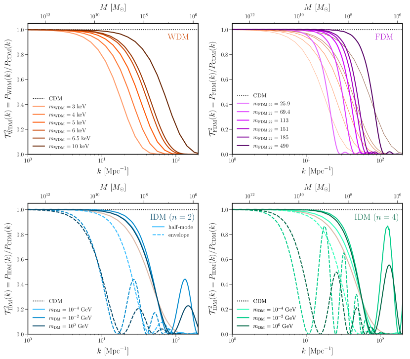
Figure 1: Ratio of the linear matter power spectrum for all beyond-CDM models represented in the COZMIC I suite. Top ticks show halo masses (in units of solar mass) associated with given wave numbers in linear theory (Equation 3). FDM models are chosen to match the half-mode wavenumber for each WDM model we simulate, which are shown as faint lines in the top-right panel (see Section 3.1.2). In the IDM panels, solid (dashed) lines show models matched to the half-mode scale of (models that are strictly more suppressed than) the $m_{\mathrm{WDM}}=6.5~{}\mathrm{keV}$ transfer function, which is shown as a faint orange line (see Section 3.1.3).

3.1.2 Fuzzy Dark Matter

To compute FDM transfer functions, we use a lightly-modified version of axionCAMB (Hlozek et al., 2015; Grin et al., 2022), described in Appendix A. We generate transfer functions for $m_{\mathrm{FDM,22}}\in[25.9,69.4,113,151,185,490]$. These values are chosen such that the corresponding half-mode scale $k_{\mathrm{hm}}$ matches that for each WDM scenario we simulate at the percent level.

Half-mode scales and de Broglie scales for these FDM models are listed in Table 1. The corresponding transfer functions in the top-right panel of Figure 1 cut off more sharply than the thermal-relic WDM models with matched half-mode scales. The impact of this difference on nonlinear modeling was noted in previous studies (e.g., Armengaud et al. 2017; Nadler et al. 2019a; Schutz 2020), and we study the effects of this difference directly in this work.

3.1.3 Interacting Dark Matter

To compute IDM transfer functions, we use a modified version of CLASS (Boddy et al., 2018; Gluscevic & Boddy, 2018). For each $m_{\mathrm{IDM}}\in[10^{-4},~{}10^{-2},~{}1]~{}\mathrm{GeV}$, we choose $\sigma_{0}$ so that the resulting transfer function either ($i$) matches the half-mode scale of the $m_{\mathrm{WDM}}=6.5~{}\mathrm{keV}$ transfer function, or ($ii$) is strictly more suppressed than the $m_{\mathrm{WDM}}=6.5~{}\mathrm{keV}$ transfer function. We refer to these as “half-mode” and “envelope” models, respectively. We choose $m_{\mathrm{WDM}}=6.5~{}\mathrm{keV}$ as a reference model because it corresponds to the current WDM bound from the MW satellite galaxy population (Nadler et al., 2021b). By comparing to this bound, Maamari et al. (2021) have shown that the envelope models are robustly disfavored by MW satellite abundances, while the half-mode models must be simulated directly to derive more stringent bounds; the latter is thus a goal of this work.

The parameters of the IDM models we simulate are summarized in Table 1, including their half-mode scales and first DAO peak characteristics. The corresponding transfer functions are shown in the bottom panels of Figure 1, featuring a variety of shapes that depend on model parameters, as discussed in previous studies (e.g., Nadler et al. 2019a; Maamari et al. 2021). In particular, we note that the DAO peak height is a non-monotonic function of $m_{\mathrm{IDM}}$, which (among the IDM parameter values we consider) reaches a maximum amplitude for $m_{\mathrm{IDM}}=10^{-2}~{}\mathrm{GeV}$ DAO features are generally more prominent for $n=4$ models.

3.1.4 Generating Zoom-in Initial Conditions

We generate ICs by passing the density and velocity transfer functions generated for each beyond-CDM scenario into MUSIC (Hahn & Abel, 2011). We use identical random seeds in all cases, such that the phases of density modes are fixed in our beyond-CDM simulations; thus, the only difference relative to CDM is that the amplitude of each mode is multiplied by $\mathcal{T}^{2}_{\mathrm{beyond-CDM}}(k)$. This procedure ensures that the same high-mass subhalos form in each scenario, and that suppression of low-mass subhalo abundances is due to $P(k)$ suppression rather than stochasticity from resampling small-scale modes.

We resimulate two Milky Way-est hosts (Halo004 and Halo113; Buch et al. 2024) and one Symphony Milky Way host (Halo023; Nadler et al. 2023). We refer to the Milky Way-est hosts as “MW–like,” because they contain LMC analog subhalos and merge with Gaia–Sausage–Enceladus (GSE) analogs; we refer to the Symphony Milky Way host as “MW–mass” because it is only constrained to have a host halo mass similar to the MW. We choose these hosts due to their small Lagrangian volumes, which makes them relatively inexpensive to resimulate. For each simulation, we initialize a region at $z=99$ that corresponds to the Lagrangian volume of particles within $10$ times the virial radius of the host halo in the parent box at $z=0$, following Nadler et al. (2023). Thus, the models we simulate do not suppress $P(k)$ on scales larger than the zoom-in region, which corresponds to a wavenumber $k_{L}=2\pi/(3~{}\mathrm{Mpc})\approx 2~{}\mathrm{Mpc}^{-1}$.

Our $72$ fiducial-resolution beyond-CDM simulations (i.e., $24$ simulations per each of our three hosts) use four refinement regions relative to the parent box, yielding an equivalent of $8192$ particle per side in the highest-resolution region and a mean interparticle spacing of $22~{}\mathrm{kpc}$, corresponding to a Nyquist frequency $k_{\mathrm{Ny}}=\pi/(22~{}\mathrm{kpc})\approx 143~{}\mathrm{Mpc}^{-1}$. For these fiducial-resolution simulations, the DM particle mass in the highest-resolution regions is $m_{\mathrm{part}}=4.0\times 10^{5}~{}M_{\mathrm{\odot}}$. We also perform $24$ high-resolution beyond-CDM simulations of one host (Halo004) using an additional refinement region; see Appendix C for details.

Figure 2 compares the distribution of density contrasts, $\delta$, for high-resolution particles in the zoom-in region for Halo004 at $z=99$ in CDM and our WDM models. Local densities are computed in Pynbody at the position of each particle with a smoothed particle hydrodynamics (SPH) kernel, using $64$ nearest neighbors. The WDM density contrast distributions are suppressed relative to CDM at both large positive and negative values of $\delta$, indicating that small-scale overdensities and underdensities are smoothed out by $P(k)$ suppression. Interestingly, even the $m_{\mathrm{WDM}}=10~{}\mathrm{keV}$ model’s overdensity distribution noticeably differs from CDM, although we will show that subhalo abundances in these models are statistically consistent above our fiducial resolution limit. The results in Figure 2 are qualitatively similar for our FDM and IDM models.

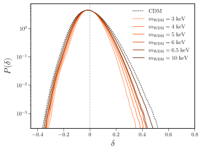
Figure 2: Distribution of local density contrast evaluated at the position of each high-resolution particle at $z=99$ in CDM (dotted black line) and each of our WDM models (solid orange lines), generated by MUSIC for one of our MW–like zoom-ins (Halo004). The dashed gray vertical line marks $\delta=0$, differentiating overdensities from underdensities. Density contrasts are computed using pynbody (Pontzen et al., 2013).

3.2 Zoom-in Simulations

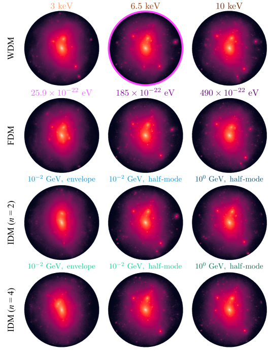
Figure 3: Projected DM density maps at $z=0$ for a subset of the high-resolution beyond-CDM simulations of a MW–like system (Halo004). For each simulation, the visualization is centered on the host halo and spans $1.5$ times its virial radius. The half-mode scale is the same for every model within each column, except for the IDM models in the left column, which correspond to envelope cross sections for $m_{\mathrm{IDM}}=10^{-2}~{}\mathrm{GeV}$ with $n=2$ (third row) and $n=4$ (fourth row). The $m_{\mathrm{WDM}}=6.5~{}\mathrm{keV}$ visualization is highlighted as a reference model used throughout the paper. Note that the $m_{\mathrm{WDM}}=10~{}\mathrm{keV}$ and $m_{\mathrm{FDM,22}}=490$ density maps are visually similar to CDM. Visualizations were created using meshoid (https://github.com/mikegrudic/meshoid).

We run the simulations using Gadget-2 (Springel, 2005). We save $236$ output snapshots per run, starting at $z\approx 10$, with a typical output cadence of $\approx 25~{}\mathrm{Myr}$ near $z=0$. We set the time stepping criterion to $\eta=0.01$ and the comoving Plummer-equivalent gravitational softening to $\epsilon=170~{}\mathrm{pc}~{}h^{-1}$, following Symphony and Milky Way-est settings (Nadler et al., 2023; Buch et al., 2024).

Figure 3 shows projected DM density maps from the high-resolution runs of a MW–like host (Halo004), for various beyond-CDM models. Even though the high-resolution region in each zoom-in extends to $\approx 10$ times the virial radius of the zoom-in host $R_{\mathrm{vir}}$, the visualizations shown in the Figure show a region spanning only $1.5R_{\mathrm{vir}}$, in order to highlight substructure. Small-scale structure is clearly suppressed in the beyond-CDM scenarios, and the amount of suppression depends on the ICs. For example, very little substructure is visible in the $m_{\mathrm{WDM}}=3~{}\mathrm{keV}$ simulation, while the $m_{\mathrm{WDM}}=6.5~{}\mathrm{keV}$ simulation only subtly differs from $m_{\mathrm{WDM}}=10~{}\mathrm{keV}$, which in turn is visually similar to CDM. At a fixed half-mode scale, substructure is visibly affected by both the slope of the transfer function (e.g., compare the WDM and FDM rows in Figure 3) and by the presence of DAOs (e.g., compare the WDM and IDM rows in Figure 3). Substructure in our envelope IDM scenarios is more suppressed than in the corresponding half-mode scenarios, which visually confirms that the IDM constraints derived in Maamari et al. (2021) are conservative. We quantify these findings below.

3.3 Post-processing and Analysis

We generate halo catalogs and merger trees by running Rockstar and consistent-trees (Behroozi et al., 2013a, b) on the highest-resolution particles from each simulation’s output snapshots. We analyze all simulations at $z=0$ to ensure that SHMF suppression relative to CDM is measured at the same cosmic time in all cases. For one of our two MW–like halos (Halo004), this matches the analysis snapshot in Buch et al. (2024).

Following the Symphony convergence tests in Nadler et al. (2023), we only analyze subhalos with at least $300$ particles at $z=0$. In our fiducial-resolution simulations, this corresponds to a virial mass threshold of $M_{\mathrm{res}}=1.2\times 10^{8}~{}M_{\mathrm{\odot}}$. Present-day SHMFs are converged above this threshold at our fiducial resolution in CDM (Nadler et al., 2023). Throughout, we calculate SHMFs using peak virial mass,

$$M_{\mathrm{sub,peak}}\equiv\max(M_{\mathrm{sub}}(z)),$$ (17)

because $M_{\mathrm{sub,peak}}$ most directly connects to the scale of the linear density perturbation that formed a given subhalo, and thus to the mass associated with a given wavenumber in linear theory (Equation 3).

However, we note that SHMFs are less well converged as a function of peak (versus present-day) mass because subhalos of a given peak mass can be heavily stripped (e.g., Nadler et al. 2023; Mansfield et al. 2024). We therefore restrict our peak SHMF measurements to subhalos above our fiducial present-day mass threshold of $M_{\mathrm{sub}}>1.2\times 10^{8}~{}M_{\mathrm{\odot}}$. In Appendix C, we show that the suppression of the peak SHMF relative to CDM that we measure is consistent between simulations of different resolution when this present-day mass cut is applied. The Symphony convergence tests in Nadler et al. (2023) indicate that subhalo maximum circular velocity ($V_{\mathrm{max}}$) functions are less well converged than mass functions. Thus, we focus on SHMFs in this paper, leaving a detailed study of subhalo $V_{\mathrm{max}}$ functions and density profiles in our beyond-CDM simulations to future work.

We do not impose additional cuts (beyond the resolution cut described above) to remove spurious halos formed through artificial fragmentation, which have hampered previous WDM simulations (e.g., Wang & White 2007). Even though we use a standard N-body code, rather than a simulation technique that mitigates artificial fragmentation (e.g., based on evolving the phase-space sheet; Angulo et al. 2013; Stücker et al. 2022), spurious objects contribute negligibly to the population of well-resolved subhalos in our simulations. Specifically, the lower limit on halo mass derived in previous studies to remove spurious halos is defined as $\kappa M_{\mathrm{lim}}$ (Lovell et al., 2014), where $\kappa\approx 0.5$. For all of our simulations, $\kappa M_{\mathrm{lim}}<M_{\mathrm{res}}$; indeed, for most of beyond-CDM models we simulate, $M_{\mathrm{lim}}\ll M_{\mathrm{res}}$. In Appendix D, we explicitly show that spurious halos contribute negligibly to subhalo populations above our fiducial resolution threshold in all beyond-CDM simulations we present based on the shapes of their protohalo particle distributions in the ICs.

4 Simulation Results

We now present COZMIC simulation results: host halo mass accretion histories (Section 4.1), SHMFs (Section 4.2), and subhalo radial distributions (Section 4.3). Appendix B summarizes key properties of each beyond-CDM simulation we present. For the remainder of the paper (except to demonstrate convergence in Appendix C), we only use our fiducial-resolution simulations. Furthermore, we exclusively study subhalos, defined as objects within the virial radius of each zoom-in host at $z=0$.

4.1 Host Halo Mass Accretion Histories

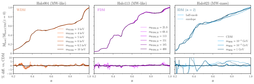
Figure 4: Host halo mass accretion histories for our MW–like hosts (left and middle panels) and MW–mass host (right panel) are shown as a function of the scale factor. In each panel, black dotted lines represent CDM, while the colored lines represent beyond-CDM models; each curve is normalized to the host mass in CDM at $z=0$. Bottom panels show the fractional differences. We note that host halo masses in beyond-CDM cosmologies match the CDM case at the percent level, at $z=0$. Note that we only show a subset of our IDM simulations here; the IDM results for $n=4$ are qualitatively similar to $n=2$ case.

Figure 4 shows host halo mass accretion histories, normalized to each host’s mass in CDM at $z=0$, for a subset of our beyond-CDM simulations. Mass accretion histories vary from host to host; in particular, the two MW–like hosts (Halo004 and Halo113) are selected to undergo an early merger with an analog of the GSE system and a recent merger with an LMC–like system. The GSE and LMC-analog mergers are reflected in these hosts’ mass accretion histories at $a\approx 0.4$ and $a\approx 1$, respectively; for details, see Buch et al. (2024). Meanwhile, the MW–mass host (Halo023) experiences an early phase of rapid growth that ends at $a\approx 0.4$, typical of MW–mass halos’ average formation histories (e.g., Wechsler et al. 2002; Lu et al. 2006; Nadler et al. 2023).

Overall, hosts in beyond-CDM models undergo very similar mass growth relative to their CDM counterparts, which is expected given that $P(k)$ is at most mildly affected on the scale of the MW hosts. In particular, all hosts’ $z=0$ masses match their CDM counterparts at the percent level. WDM, FDM, and half-mode IDM hosts’ mass accretion histories further match CDM to within $\approx 5\%$ at all redshifts where they are well resolved, with the only differences noticeable at very early times. Meanwhile, in our envelope IDM models, mass accretion histories differ at the $\approx 10\%$ level from their CDM counterparts at early times for $m_{\mathrm{IDM}}=10^{-2}~{}\mathrm{GeV}$ and $m_{\mathrm{IDM}}=1~{}\mathrm{GeV}$. Nonetheless, these hosts’ masses eventually converge to their CDM counterparts.

We also measure virial concentrations of host halos $c_{\mathrm{vir}}\equiv R_{\mathrm{vir}}/R_{s}$, where $R_{s}$ is the Navarro–Frenk–White (NFW; Navarro et al. 1997) scale radius. We find that $z=0$ concentrations in most beyond-CDM simulations match those in CDM at the percent level. The most notable exceptions are: i) the most suppressed FDM model we consider (with $m_{\mathrm{FDM,22}}=25.9$), and ii) the IDM envelope scenario, for which $c_{\mathrm{vir}}$ is increased by $\gtrsim 10\%$ relative to CDM; see Appendix B for details. Certain FDM and WDM cases with similar half-mode scales (e.g., $m_{\mathrm{FDM,22}}=25.9$ and $m_{\mathrm{WDM}}=3~{}\mathrm{keV}$) yield different values of $c_{\mathrm{vir}}$, which could indicate that host concentration is sensitive to the shape of the transfer function; this would agree with previous findings using cosmological simulations (e.g., Brown et al. 2020). We leave a study of halo and subhalo density profiles in our beyond-CDM simulations to future work.

4.2 Subhalo Mass Functions

Figure 5: Cumulative SHMFs, averaged over our three MW hosts, shown in four different beyond-CDM cosmologies (solid colored lines) and in CDM (dotted black lines). We only consider subhalos with present-day virial masses $M_{\mathrm{sub}}>1.2\times 10^{8}~{}M_{\mathrm{\odot}}$, corresponding to $>300$ particles in the fiducial-resolution simulations. FDM models and WDM models have matching half-mode scales. WDM models are shown in the FDM panel as faint lines, for comparison (see Section 3.1.2). In the IDM panels, solid lines show models that have the same half-mode scale as the limiting WDM case $m_{\mathrm{WDM}}=6.5~{}\mathrm{keV}$, while the dashed lines show IDM models where the transfer function is strictly more suppressed at all $k$. The SHMF for the limiting WDM model is shown as a faint line in both bottom panels for comparison (see Section 3.1.3). Markers indicate the half-mode masses of the most extreme models in each panel (in the IDM panels, markers correspond to envelope models); the half-mode masses for less extreme models are below $10^{8}~{}M_{\mathrm{\odot}}$. Dark gray bands show the $1\sigma$ Poisson uncertainty on the mean cumulative CDM SHMF, and light gray bands show the range of host-to-host variation.

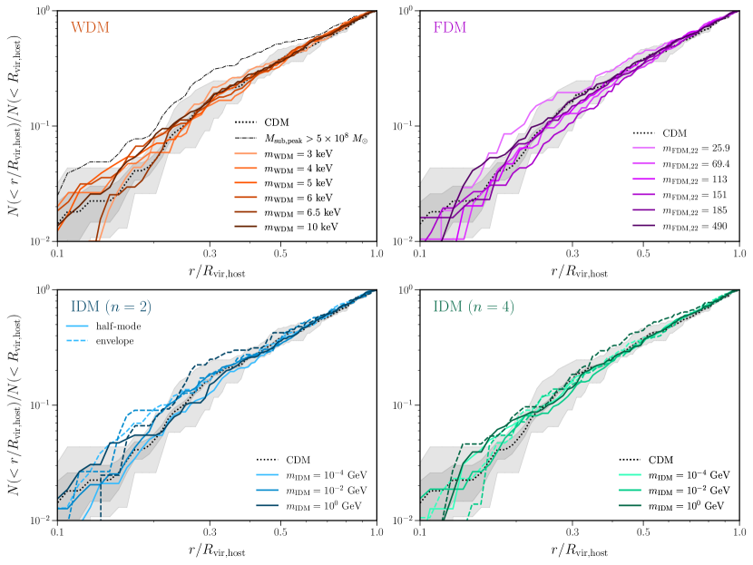
Figure 6: Mean subhalo radial distributions, averaged over our three MW hosts, in beyond-CDM cosmologies (solid colored lines) and in CDM (dotted black lines). Each radial distribution is normalized to the total number of subhalos within $R_{\mathrm{vir,host}}$. All results are restricted to subhalos with present-day virial masses $M_{\mathrm{sub}}>1.2\times 10^{8}~{}M_{\mathrm{\odot}}$ except for the dot-dashed line in the top-left panel, which shows the CDM radial distribution for subhalos with $M_{\mathrm{sub,peak}}>5\times 10^{8}~{}M_{\mathrm{\odot}}$. In the IDM panels, solid (dashed) lines show models with $P(k)$ matched to the half-mode scale of (strictly more suppressed than) the $m_{\mathrm{WDM}}=6.5~{}\mathrm{keV}$ model. Dark gray bands show the $1\sigma$ Poisson uncertainty on the mean normalized radial distribution, and light gray bands show the range of host-to-host variation.

At $z=0$, we identify 93, 77, and 69 subhalos above our $M_{\mathrm{sub}}>1.2\times 10^{8}~{}M_{\mathrm{\odot}}$ resolution threshold in the Halo004, Halo113, and Halo023 CDM runs, respectively. In beyond-CDM cosmologies, total subhalo counts are very sensitive to the specific beyond-CDM model parameters used in a given simulation. For example, above the same present-day virial mass threshold in Halo004, we identify 40, 66, and 79 subhalos for WDM with $m_{\mathrm{WDM}}=3$, $5$, and $6.5~{}\mathrm{keV}$, respectively. Holding each half-mode scale fixed while changing the shape of the power spectrum has a notable effect on the subhalo population. For example, examining FDM cosmologies with the same half-mode scale as the WDM cosmologies above (namely, $m_{\mathrm{FDM,22}}=25.9$, $113$, and $185$), we identify 36, 82, and 95 subhalos, respectively. Fixing the half-mode scale to our $m_{\mathrm{WDM}}=6.5~{}\mathrm{keV}$ model and introducing DAOs along with a steeper initial cutoff in IDM models, we find 84, 85, and 83 subhalos for $n=4$ the half-mode case with $m_{\mathrm{IDM}}=10^{-4}$, $10^{-2}$, and $1~{}\mathrm{GeV}$. Meanwhile, $n=4$ envelope IDM cases that suppress $P(k)$ strictly more than WDM with $m_{\mathrm{WDM}}=6.5~{}\mathrm{keV}$ yield 63, 53, and 42 subhalos for the same IDM benchmark masses, respectively. The latter comparison is particularly striking, as the $m_{\mathrm{IDM}}=10^{-2}~{}\mathrm{GeV}$ envelope run has a smaller $k_{\mathrm{hm}}$ than the $m_{\mathrm{IDM}}=1~{}\mathrm{GeV}$ run, yet forms more substructure because of its prominent DAOs. We expand on this when modeling SHMF suppression in Section 5.

To assess the statistical significance of the differences in subhalo population we observe for different beyond-CDM scenarios, Figure 5 shows SHMFs averaged over the three MW hosts, along with the associated Poisson uncertainty on the CDM SHMF (dark bands) and the range of host-to-host scatter (light bands). We find that subhalo abundances are clearly suppressed at the low-mass end in all of our beyond-CDM simulations. For a number of models, the suppression is statistically significant, exceeding both the Poisson uncertainty on the mean CDM SHMF at the lowest mass resolved, $M_{\mathrm{sub,peak}}\approx 10^{8}~{}M_{\mathrm{\odot}}$, as well as the variation across our three hosts. Furthermore, some models significantly suppress subhalo abundances up to $M_{\mathrm{sub,peak}}\approx 10^{10}~{}M_{\mathrm{\odot}}$. The amount of suppression is determined by $P(k)$, such that models with lower WDM masses, lower FDM masses, and higher IDM cross sections (at fixed $m_{\mathrm{IDM}}$) yield fewer total subhalos. Subhalo abundances are most heavily suppressed below the halo mass corresponding to each model’s half-mode wavenumber; the corresponding half-mode mass is indicated by the triangle markers in Figure 5. However, even for cases where $M_{\mathrm{hm}}<10^{8}~{}M_{\mathrm{\odot}}$, SHMF suppression can be significant at the lowest $M_{\mathrm{sub,peak}}$ resolved, as shown in Figure 5.

Beyond the overall amplitude of the suppression, we find that the shape of $P(k)$ affects the shape of the corresponding SHMF, as illustrated in Figure 5. For example, all FDM models (with a notable exception of the most extreme case) yield more subhalos than WDM models with the same half-mode scales. Meanwhile, IDM scenarios with the same half-mode scale as an $m_{\mathrm{WDM}}=6.5~{}\mathrm{keV}$ model yield slightly higher subhalo abundances, suggesting that either the slope of the suppression, or the DAOs in $P(k)$ (at $k>k_{\mathrm{hm}}$), can reduce the suppression. On the other hand, SHMFs in our envelope IDM models are heavily suppressed, even at relatively high $M_{\mathrm{sub,peak}}$. Among the beyond-CDM models we consider, the shape of the SHMF is most distinct from that in CDM for the envelope IDM scenarios. We interpret all of these findings in Section 5 by modeling the suppression of the SHMF relative to CDM in WDM and FDM cosmologies, and by comparing IDM results to the other beyond-CDM scenarios.

At $M_{\mathrm{sub,peak}}\gtrsim 10^{10}~{}M_{\mathrm{\odot}}$, beyond-CDM SHMFs are consistent with CDM within the Poisson uncertainty, except for certain envelope IDM models. In some cases (e.g., the $m_{\mathrm{WDM}}=6~{}\mathrm{keV}$ model in the top-left panel of Figure 5), beyond-CDM simulations have a few more high-mass subhalos than CDM, which may be related to orbital phase shifts discussed below. For $M_{\mathrm{sub,peak}}\gtrsim 3\times 10^{10}~{}M_{\mathrm{\odot}}$, beyond-CDM SHMFs converge to the CDM result. Furthermore, the masses of LMC analogs are nearly identical in all simulations.

All of these qualitative findings hold when the present-day halo masses are used to measure SHMFs, rather than peak virial masses. Furthermore, SHMFs are converged as a function of simulation resolution (see Appendix C). Note that Figure 5 supports our claim from Section 3.3 that spurious halos do not significantly impact our results, since the cumulative SHMF stops increasing significantly for $M_{\mathrm{sub,peak}}\lesssim 2\times 10^{8}~{}M_{\mathrm{\odot}}$ and flattens for both CDM and all beyond-CDM models shown here. This flattening is largely due to the cut on present-day subhalo mass, since surviving subhalos are typically tidally stripped in mass by a factor of $\gtrsim 2$ relative to their peak mass (e.g., Nadler et al. 2023).

4.3 Subhalo Radial Distributions

Figure 6 shows subhalo radial distributions averaged over our three MW hosts. Before averaging, we normalize each radial distribution to the total number of subhalos within the corresponding host’s virial radius, in order to highlight trends in the shape (since the total subhalo abundance differs in different beyond-CDM models). We apply the fiducial cut of $M_{\mathrm{sub}}>1.2\times 10^{8}~{}M_{\mathrm{\odot}}$ in all cases. The hosts all have virial radii of $R_{\mathrm{vir,host}}\approx 300~{}\mathrm{kpc}$, such that $r/R_{\mathrm{vir,host}}=0.1$, $0.3$, and $0.5$ roughly correspond to distances of $30$, $100$, and $150~{}\mathrm{kpc}$.

Normalized radial distributions in most of our beyond-CDM simulations converge to the CDM result for $r/R_{\mathrm{vir,host}}\gtrsim 0.3$. For $r/R_{\mathrm{vir,host}}\lesssim 0.3$, certain beyond-CDM radial distributions are more concentrated than in CDM, though the difference does not exceed the host-to-host scatter at any fixed radial distance. Since the abundances of low-mass subhalos are reduced in beyond-CDM cosmologies, and since the more massive subhalos tends to be more concentrated toward the center of the host (e.g., Nagai & Kravtsov 2005; Kravtsov 2010; Nadler et al. 2023), the mild enhancement of the inner radial distribution visible in some of the models could be a combination of these two effects. To illustrate this mass dependence the top-left panel of Figure 6 shows the radial distribution of subhalos with $M_{\mathrm{sub,peak}}>5\times 10^{8}~{}M_{\mathrm{\odot}}$ in CDM. This yields a more concentrated radial distribution, confirming previous results.

We note that radial distributions for individual resimulated hosts can be noisy due to stochastic changes in subhalo orbits. In particular, particle trajectories in cosmological simulations are potentially chaotic (a form of the ‘butterfly effect’; Genel et al. 2019); similar behavior has been noted for subhalo orbits in previous studies, even when the same host is resimulated in a fixed model at different resolution levels (e.g., Frenk et al. 1999; Springel et al. 2008). This kind of stochasticity may partly explain the non-monotonic relation between radial distribution shape and the severity of beyond-CDM suppression shown in Figure 6. Radial distributions can also be affected by orbital phase shifts of matched subhalo pairs that experience different gravitational potentials after falling into the MW host. However, density profiles of our MW hosts are not significantly altered relative to CDM, except in the most extreme beyond-CDM models (i.e., the envelope IDM scenarios).

To further unpack our radial distribution results, we match subhalos among our simulations, based on their pre-infall mass accretion histories and orbits, regardless of whether they survive to $z=0$. The most massive subhalos in our beyond-CDM simulations have orbits nearly identical to their CDM counterparts. While the orbital phases of lower-mass subhalos often shift, the resulting differences in present-day distance are not systematic and mainly introduce scatter in the comparison between CDM and beyond-CDM radial distributions. Thus, the radial distribution differences we identify are due to the suppression of low-mass subhalo abundances in beyond-CDM scenarios rather than differences in the orbits of matched subhalo pairs. Consistent with this result, Lovell et al. (2021) find that WDM radial distributions are more concentrated in CDM at sufficiently low infall masses, indicating that recently-accreted, low-mass CDM subhalos are largely responsible for this difference.

5 Modeling Subhalo Mass Functions Beyond CDM

In this Section, we treat the COZMIC suite as “data” that provides measurements of the SHMF in beyond-CDM scenarios. We present a parametric model for the SHMF and perform probabilistic inference to reconstruct model parameters that fit simulated data; we report the full posterior probability distributions of model parameters for each beyond-CDM scenario captured by COZMIC. We describe the SHMF model and the Poisson likelihood procedure in Section 5.1; we present the results for WDM in Section 5.2, for FDM in Section 5.3, and for IDM in Section 5.4, and compare them to previous studies.

We emphasize three key advances of our SHMF modeling approach, relative to previous studies. First, we measure SHMF suppression using peak subhalo mass, rather than the present-day mass, because $M_{\mathrm{sub,peak}}$ more directly traces the relevant scales in $P(k)$. Second, we explicitly model the effect of stripping below our simulations’ present-day mass resolution limit as a function of $M_{\mathrm{sub,peak}}$. As a result, our SHMF models are only fit down to $M_{\mathrm{sub,peak}}=1.2\times 10^{8}~{}M_{\mathrm{\odot}}$ (note that this is slightly below the minimum peak halo mass of currently-observed MW satellite galaxies; Nadler et al. 2020). Third, we fit the model probabilistically to our simulation data and report the resulting uncertainties in the model parameters, along with the list of best-fit values.

5.1 Subhalo Mass Function Model

We write the differential SHMF in host $i$ and beyond-CDM scenario $j$ as

$$\frac{\mathrm{d}N_{ij}(\Theta)}{\mathrm{d}\log(M_{\mathrm{sub,peak}})} =\left(\frac{a_{i}}{100}\right)\left(\frac{M_{\mathrm{sub,peak}}}{M_{\mathrm{host,}ij}}\right)^{-b_{i}}e^{-50\left(\frac{M_{\mathrm{sub,peak}}}{M_{\mathrm{host,}ij}}\right)^{4}}$$

$$\times p_{ij}(M_{\mathrm{sub}}>M_{\mathrm{min}}\lvert M_{\mathrm{sub,peak}})$$

$$\times f_{\mathrm{beyond-CDM}}(M_{\mathrm{sub,peak}},\theta_{j},\alpha,\beta,\gamma),$$ (18)

where $\vec{\Theta}=\{a_{i},~{}b_{i},~{}\alpha,~{}\beta,~{}\gamma\,~{}\theta_{j}\}$. The first three terms model the CDM SHMF following van den Bosch & Jiang (2016), where the normalization $a_{i}$ and power-law slope $b_{i}$ are free parameters. The fourth term models the probability that a subhalo with a given $M_{\mathrm{sub,peak}}$ has a present-day virial mass $M_{\mathrm{sub}}$ above the resolution limit, $M_{\mathrm{min}}=M_{\mathrm{res}}=1.2\times 10^{8}~{}M_{\mathrm{\odot}}$, and is therefore accounted for in our measurements of the SHMF from simulations; thus, this term models the effects of the simulation resolution limit on derived SHMFs measured using $M_{\mathrm{peak,sub}}$. For each host and DM scenario, we use the simulated subhalo population to reconstruct the joint probability distribution of $M_{\mathrm{sub}}$ and $M_{\mathrm{sub,peak}}$. We use kernel density estimation (KDE) for this purpose, which allows us to integrate the normalized KDE above $M_{\mathrm{min}}$ and recover the probability that a subhalo is stripped below the resolution limit as a function of $M_{\mathrm{sub,peak}}$.

The final term in Equation 18 models the SHMF suppression relative to CDM, which depends on a parameter $\theta$ specific to each beyond-CDM scenario (i.e., $m_{\mathrm{WDM}}$ or $m_{\mathrm{FDM}}$). We adopt a model that was previously shown to describe halo and subhalo mass function suppression accurately in WDM and FDM (e.g., Lovell 2020b; Benito et al. 2020),

$$f_{\mathrm{beyond-CDM}}(M_{\mathrm{sub,peak}},\theta,\alpha,\beta,\gamma)=\left[1+\left(\frac{\alpha M_{\mathrm{hm}}(\theta)}{M_{\mathrm{sub,peak}}}\right)^{\beta}\right]^{-\gamma},$$ (19)

where $M_{\mathrm{hm}}(\theta)$ is the half-mode mass and $\alpha$, $\beta$, and $\gamma$ are free parameters. In the following, we show that a single distribution of $\{\alpha,\beta,\gamma\}$ accurately describes all WDM models, while a different distribution describes the FDM scenarios.

For each beyond-CDM scenario, we fit the model defined by Equation 18 to our simulations, using a Poisson likelihood that describes the probability of measuring a set of subhalos with peak subhalo masses $M_{\mathrm{sub,peak}}$ and present-day masses $M_{\mathrm{sub}}>M_{\mathrm{min}}$. Specifically, the likelihood function reads

$$\mathcal{L}(\vec{\Theta})=\prod_{i}^{N_{\mathrm{hosts}}}\prod_{j}^{N_{\mathrm{models}}}\mathrm{Pois}(N_{\mathrm{sim,}ij}\lvert N_{ij}(\vec{\Theta}))\prod_{k}^{N_{\mathrm{sim,}ij}}P_{ij}(M_{\mathrm{sub,peak,}k}\lvert\vec{\Theta})$$

$$=\prod_{i}^{N_{\mathrm{hosts}}}\prod_{j}^{N_{\mathrm{models}}}\frac{N_{ij}(\vec{\Theta})^{N_{\mathrm{sim,}ij}}e^{-N_{ij}(\vec{\Theta})}}{N_{\mathrm{sim,}ij}!}\prod_{k}^{N_{\mathrm{sim,}ij}}\frac{\left(\frac{\mathrm{d}N_{ij}(\vec{\Theta})}{\mathrm{d}\log M_{\mathrm{sub,peak}}}\right)\big{\rvert}_{M_{\mathrm{sub,peak,}k}}}{\int\frac{\mathrm{d}N_{ij}(\vec{\Theta})}{\mathrm{d}\log M_{\mathrm{sub,peak}}}~{}\mathrm{d}\log M_{\mathrm{sub,peak}}}$$

$$=\prod_{i}^{N_{\mathrm{hosts}}}\prod_{j}^{N_{\mathrm{models}}}\frac{e^{-N_{ij}(\vec{\Theta})}}{N_{\mathrm{sim,}ij}!}\prod_{k}^{N_{\mathrm{sim,}ij}}\left(\frac{\mathrm{d}N_{ij}(\vec{\Theta})}{\mathrm{d}\log M_{\mathrm{sub,peak}}}\right)\bigg{\rvert}_{M_{\mathrm{sub,peak,}k}}.$$ (20)

Here $N_{\mathrm{sim},ij}$ is the total number of subhalos in a given simulation, appearing above the present-day mass resolution limit, in the host $i$, for DM scenario $j$. $P_{ij}(M_{\mathrm{sub,peak,}k}\lvert\vec{\Theta})$ is the probability of finding a subhalo with a specific mass of $M_{\mathrm{sub,peak,}k}$, for a given parameter vector $\vec{\Theta}$ (Equation 18). Finally,

$$N_{ij}(\vec{\Theta})\equiv\int(\mathrm{d}N_{ij}(\vec{\Theta})/\mathrm{d}\log M_{\mathrm{sub,peak}})~{}\mathrm{d}\log M_{\mathrm{sub,peak}}$$ (21)

is the expected total number of subhalos for a given $\vec{\Theta}$.

Taking the logarithm of Equation 20 yields

$$\ln\mathcal{L}(\vec{\Theta}) =-N_{\mathrm{tot}}(\vec{\Theta})-\sum_{i}^{N_{\mathrm{hosts}}}\sum_{j}^{N_{\mathrm{models}}}\ln(N_{\mathrm{sim,}ij}!)$$

$$+\sum_{i}^{N_{\mathrm{hosts}}}\sum_{j}^{N_{\mathrm{models}}}\sum_{k}^{N_{\mathrm{sim,}ij}}\ln\left(\frac{\mathrm{d}N_{ij}(\vec{\Theta})}{\mathrm{d}\log M_{\mathrm{sub,peak}}}\right)\bigg{\rvert}_{M_{\mathrm{sub,peak,}k}},$$ (22)

where $N_{\mathrm{sim,tot}}=\sum_{i}^{N_{\mathrm{hosts}}}\sum_{j}^{N_{\mathrm{models}}}N_{\mathrm{sim,}ij}$ is the total number of simulated subhalos above $M_{\mathrm{res}}$ across all hosts and DM models. The posterior probability distribution for $\vec{\Theta}$ is given by Bayes’ theorem,

$$P(\vec{\Theta}\lvert\vec{M}_{\mathrm{sub,peak}})=\frac{P(\vec{M}_{\mathrm{sub,peak}}\lvert\vec{\Theta})P(\vec{\Theta})}{P(\vec{M}_{\mathrm{sub,peak}})},$$ (23)

where $\vec{M}_{\mathrm{sub,peak}}$ represents the set of $M_{\mathrm{sub,peak}}$ values across all hosts and beyond-CDM models and $P(\vec{M}_{\mathrm{sub,peak}}\lvert\vec{\Theta})\equiv\mathcal{L}(\vec{\Theta})$, while $P(\vec{\Theta})$ represents the prior probability for each model parameter. For both our FDM and WDM fits, we implement linear uniform prior probability distributions for the normalizations $0.1<a_{i}<10$ and $0<\alpha<50$, and Jeffreys priors for the slopes $0.1<b_{i}<1.5$, $0<\beta<10$, and $0<\gamma<5$. We sample the nine-dimensional posterior in Equation 23 by running the Markov Chain Monte Carlo (MCMC) sampler emcee (Foreman-Mackey et al., 2013) for $10^{5}$ steps with $100$ walkers, discarding $10^{4}$ burn-in steps. This yields well-converged posteriors with hundreds of independent samples, shown in Figures 7 and 9.

We ultimately marginalize over $a_{i}$ and $b_{i}$ to infer posterior distributions for $\{\alpha,~{}\beta,~{}\gamma\}$, thereby capturing covariances between these parameters. Because of the significant difference in SHMF shapes, we perform separate inference of the SHMF model parameters for WDM and for FDM. We include the CDM simulations in the likelihood for each scenario because CDM is captured in the $f_{\mathrm{beyond-CDM}}\rightarrow 1$ limit. For IDM, we compare SHMF suppression to WDM models that produce matching total subhalo abundances and assess the impact of DAOs and the transfer function cutoff shape on the resulting suppression. In Appendix E, we demonstrate that our three hosts yield consistent posteriors for the SHMF suppression parameters, and we quantify host-to-host variations in the normalizations $a_{i}$ and slopes $b_{i}$.

5.2 Warm Dark Matter

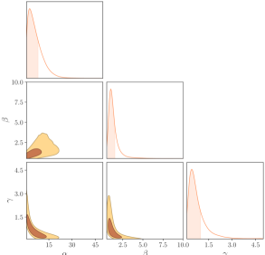
Figure 7: Marginalized posterior for our WDM SHMF suppression model. Dark (light) two-dimensional contours show $68\%$ ($95\%$) confidence intervals; top and side panels show marginal posteriors with shaded $68\%$ confidence intervals.

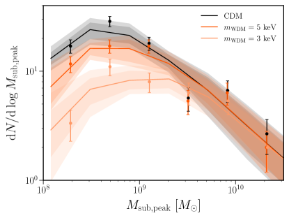
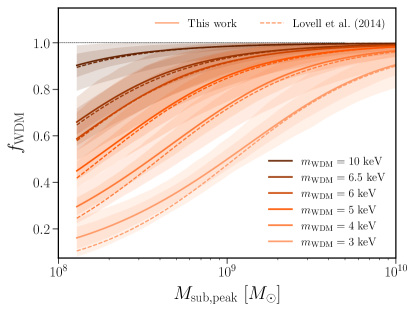
Figure 8: Left: Differential SHMF as a function of peak virial mass, measured as the mean over the three host halos simulated in this work, for WDM models with $m_{\mathrm{WDM}}=3~{}\mathrm{keV}$ (light orange), $5~{}\mathrm{keV}$ (orange), and CDM (black). Error bars show the $1\sigma$ Poisson error on the mean. Right: Corresponding SHMF Suppression functions derived from our likelihood analysis (solid lines and bands) compared to the Lovell et al. (2014) model (dashed lines). In both panels, dark (light) bands show $68\%$ ($95\%$) confidence intervals around the best-fit model.

We define WDM SHMF suppression by inserting $M_{\mathrm{hm}}(m_{\mathrm{WDM}})$ (Equation 6) into Equation 19. The resulting posterior, marginalized over the normalizations $a_{i}$ and slopes $b_{i}$, is shown in Figure 7. We infer $\alpha_{\mathrm{WDM}}=2.1^{+5.9}_{-1.9}$, $\beta_{\mathrm{WDM}}=1.0^{+0.5}_{-0.3}$, and $\gamma_{\mathrm{WDM}}=0.4^{+0.6}_{-0.3}$ at $68\%$ confidence. All three parameters have upper bounds, but $\alpha_{\mathrm{WDM}}$ and $\beta_{\mathrm{WDM}}$ are only constrained at the $\approx 1\sigma$ level from below. The best-fit parameters that maximize our posterior probability distribution are as follows:

$$\alpha_{\mathrm{WDM}}=2.5,$$

$$\beta_{\mathrm{WDM}}=0.9,$$

$$\gamma_{\mathrm{WDM}}=1.0.$$ (24)

The inferred values of $\alpha_{\mathrm{WDM}}$, $\beta_{\mathrm{WDM}}$, and $\gamma_{\mathrm{WDM}}$ are consistent with previous measurements of the WDM SHMF suppression from Lovell et al. (2014), which reported $\alpha_{\mathrm{WDM}}=2.7$, $\beta_{\mathrm{WDM}}=1$, $\gamma_{\mathrm{WDM}}=0.99$. We discuss other results from the WDM literature below and in Section 7.

Studies that model the WDM SHMF suppression routinely report a single set of best-fit values for $\alpha_{\mathrm{WDM}}$, $\beta_{\mathrm{WDM}}$, and $\gamma_{\mathrm{WDM}}$ (e.g., Lovell et al. 2014; Lovell 2020b). However, as shown by Figure 7, we find significant uncertainties on parameter values, as well as correlations between parameters; this holds even though we use a relatively large collection of WDM zoom-in simulations to constrain the SHMF model. The uncertainty is particularly large for $\alpha_{\mathrm{WDM}}$, which controls the mass scale of the SHMF suppression onset. This is partially due to a degeneracy with $\gamma_{\mathrm{WDM}}$, which controls the slope of the suppression for $M_{\mathrm{sub,peak}}\lesssim\alpha_{\mathrm{WDM}}M_{\mathrm{hm}}(m_{\mathrm{WDM}})$. In particular, a less steep suppression (smaller $\gamma_{\mathrm{WDM}}$) is degenerate with an earlier onset of suppression (at higher halo masses and larger $\alpha_{\mathrm{WDM}}$). In turn, the asymptotic slope is given by $\beta_{\mathrm{WDM}}\times\gamma_{\mathrm{WDM}}$, and thus $\gamma_{\mathrm{WDM}}$ is degenerate with $\beta_{\mathrm{WDM}}$.

The left panel of Figure 8 illustrates the best-fit SHMF model and its suppression function, as well as the associated uncertainties. We find that the model describes simulation data well: the reduced-$\chi^{2}$ statistic for each model (assuming Poisson errors on the simulation measurements) is $\chi^{2}=[0.76,~{}0.72,~{}0.73,~{}1.1,~{}1.0,~{}0.72]$ for $m_{\mathrm{WDM}}=[3,~{}4,~{}5,~{}6,~{}6.5,~{}10]~{}\mathrm{keV}$, respectively, indicating a good fit in all cases. Note that the differential SHMF turns over at low $M_{\mathrm{sub,peak}}$, even in CDM, due to our $M_{\mathrm{sub}}$ resolution cut. As $m_{\mathrm{WDM}}$ increases, the SHMF suppression becomes less severe (at fixed $M_{\mathrm{sub,peak}}$) and flatter (as a function of $M_{\mathrm{sub,peak}}$).

We directly compare our results with Lovell et al. (2014), derived from a suite of four thermal-relic WDM zoom-in simulations with comparable resolution to ours. Specifically, this previous study fixed $\beta_{\mathrm{WDM}}=1$ and showed that $\alpha_{\mathrm{WDM}}=2.7$, $\gamma_{\mathrm{WDM}}=0.99$ accurately describes the SHMF suppression in their simulations, measured using present-day subhalo mass. As shown by the dashed lines in the right panel of Figure 8, our $f_{\mathrm{WDM}}$ posteriors agree well with the Lovell et al. (2014) fit. Our predictions are slightly less suppressed at $10^{8}~{}M_{\mathrm{\odot}}\lesssim M_{\mathrm{sub,peak}}\lesssim 10^{9}~{}M_{\mathrm{\odot}}$ for $m_{\mathrm{WDM}}\leq 5~{}\mathrm{keV}$, although the difference is within the $1\sigma$ uncertainties of our model.

We have also compared our results with the (sub)halo mass function suppression fits from Lovell (2020b) and Stücker et al. (2022). Interestingly, our $f_{\mathrm{WDM}}$ fit agrees well with the isolated halo mass function suppression from Lovell et al. (2020b; i.e., $\alpha_{\mathrm{WDM}}=2.3,\ \beta_{\mathrm{WDM}}=0.8,\ \gamma_{\mathrm{WDM}}=1.0$), while their SHMFs are significantly less suppressed than ours (i.e., $\alpha_{\mathrm{WDM}}=4.2,\ \beta_{\mathrm{WDM}}=2.5,\ \gamma_{\mathrm{WDM}}=0.2$), even after accounting for the uncertainty on our $f_{\mathrm{WDM}}$ reconstruction (see Section 4.3 of Stücker et al. 2022 for a related discussion). Meanwhile, Stücker et al. (2022) simulate WDM-like transfer function cutoffs using a hybrid phase-space sheet plus N-body simulation technique. Instead of fitting for $\alpha_{\mathrm{WDM}}$, $\beta_{\mathrm{WDM}}$, and $\gamma_{\mathrm{WDM}}$, these authors infer the mass scales at which the halo mass function is suppressed by $20\%$, $50\%$, and $80\%$ relative to CDM. Both the halo and subhalo mass function suppression models from Stücker et al. (2022) are significantly less suppressed than our result.

We caution that these comparisons have subtleties that may have an impact; in particular, Lovell (2020b) simulated sterile neutrino WDM transfer functions, which differ from $P(k)$ in our thermal-relic WDM models (e.g., see Figure 1 of Lovell 2020a), while Stücker et al. (2022) simulated generalized $\alpha$–$\beta$–$\gamma$ transfer functions following Murgia et al. (2017), which differ from our transfer functions in detail. Furthermore, Lovell (2020b) ran cosmological WDM simulations in addition to zoom-ins, while Stücker et al. (2022) exclusively ran cosmological simulations. Thus, our comparison to Lovell et al. (2014) is the most straightforward in terms of both ICs and simulation technique. It is interesting that we obtain good agreement with Lovell et al. (2014) despite our use of peak (rather than present-day) subhalo mass. Indeed, we infer a similar $f_{\mathrm{WDM}}$ when the SHMF is measured using present-day mass, suggesting that the mass loss rates of surviving, well-resolved subhalos do not significantly differ between our CDM and WDM simulations.

5.3 Fuzzy Dark Matter

We define FDM SHMF suppression by inserting $M_{\mathrm{hm}}(m_{\mathrm{FDM,22}})$ (Equation 11) into Equation 19. The marginalized posterior for our FDM SHMF suppression parameters is shown in Figure 9. We infer $\alpha_{\mathrm{FDM}}=6.2^{+1.6}_{-2.5}$, $\beta_{\mathrm{FDM}}=1.8^{+1.9}_{-0.7}$, and $\gamma_{\mathrm{FDM}}=0.2^{+0.3}_{-0.1}$ at $68\%$ confidence. These parameters are bounded from above but are only marginally constrained from below, and they display the same qualitative degeneracies as in our WDM fit. We again provide the best-fit parameters that maximize our FDM SHMF posterior:

$$\alpha_{\mathrm{FDM}}=5.5$$

$$\beta_{\mathrm{FDM}}=2.5,$$

$$\gamma_{\mathrm{FDM}}=0.3.$$ (25)

Note that authors often define FDM SHMF suppression using Equation 19 with $M_{0}\approx M_{\mathrm{hm}}/3$ in place of $M_{\mathrm{hm}}$ (see Section 2.2). This choice would correspondingly decrease our inferred values of $\alpha_{\mathrm{FDM}}$ by a factor of $\approx 3$.

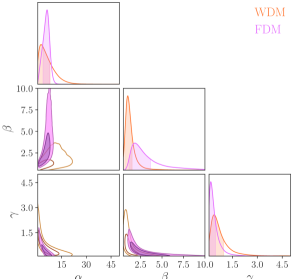
Figure 9: Marginalized posterior for our FDM SHMF suppression model (filled purple). Dark (light) two-dimensional contours show $68\%$ ($95\%$) confidence intervals; top and side panels show marginal posteriors with shaded $68\%$ confidence intervals. The WDM posterior from Figure 7 is shown for reference (unfilled orange).

Figure 10 shows our FDM SHMF fits, which again provides a good fit to our simulation results, with $\chi^{2}=[0.43,~{}0.74,~{}0.93,~{}0.69,~{}1.2,~{}0.61]$ for $m_{\mathrm{FDM,22}}=[25.9,~{}69.4,~{}113,~{}151,~{}185,~{}490]$. The inferred SHMF becomes less suppressed (at fixed $M_{\mathrm{sub,peak}}$) and flatter (as a function of $M_{\mathrm{sub,peak}}$) as $m_{\mathrm{FDM,22}}$ increases. In comparison to our WDM results, we find that:

• The best-fit value of $\alpha_{\mathrm{FDM}}$ is larger than $\alpha_{\mathrm{WDM}}$ by a factor of $\approx 2$; however, the marginalized posteriors are consistent at the $1\sigma$ level;

• The best-fit value of $\beta_{\mathrm{FDM}}$ is larger than $\beta_{\mathrm{WDM}}$ by a factor of $\approx 3$, corresponding to a $1\sigma$ shift in the marginalized posteriors, indicating that FDM SHMF suppression is steeper than in WDM;

• The best-fit values and marginalized posteriors for $\gamma_{\mathrm{FDM}}$ and $\gamma_{\mathrm{WDM}}$ are statistically consistent.

• Half mode-matched FDM and WDM models yield consistent suppression at $M_{\mathrm{sub,peak}}=10^{8}~{}M_{\mathrm{{\odot}}}$. For each half mode-matched pair, the probability that we draw an $f_{\mathrm{FDM}}(M_{\mathrm{sub,peak}}=10^{8}~{}M_{\mathrm{\odot}})$ consistent with our inferred $f_{\mathrm{WDM}}(M_{\mathrm{sub,peak}}=10^{8}~{}M_{\mathrm{\odot}})$ at the $1\sigma$ level is $p=0.09,~{}0.4,~{}0.08,~{}0.14,~{}0.11$, and $0.18$, for $m_{\mathrm{FDM,22}}=25.9,~{}69.4,~{}113,~{}151,~{}185$, and $490$, respectively.

  

  

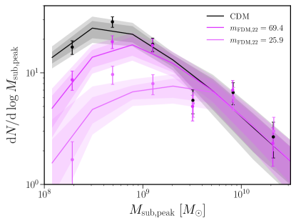
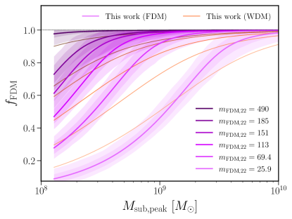
  Figure 10: Same as Figure 8, for our FDM SHMF model. In the right panel, FDM SHMF suppression functions are compared to WDM models with matched half-mode wavenumbers (faint orange lines).

• At $M_{\mathrm{sub,peak}}=10^{9}~{}M_{\mathrm{\odot}}$, the same procedure yields $p=0.16,~{}0.03,~{}0.04,~{}0.1,~{}0.13$, and $0.21$ for $m_{\mathrm{FDM,22}}=25.9,~{}69.4,~{}113,~{}151,~{}185$, and $490$, respectively. Thus, the suppression significantly differs at $M_{\mathrm{sub,peak}}=10^{9}~{}M_{\mathrm{\odot}}$ between $m_{\mathrm{FDM,22}}=69.4$ and $m_{\mathrm{WDM}}=4~{}\mathrm{keV}$, and between $m_{\mathrm{FDM,22}}=113$ and $m_{\mathrm{WDM}}=5~{}\mathrm{keV}$.

• All half mode-matched models yield suppression consistent at the $2\sigma$ level at both of these mass scales; however, two-sample KS tests using our $f_{\mathrm{FDM}}$ and $f_{\mathrm{WDM}}$ posteriors indicate significant differences between the distributions at each $M_{\mathrm{sub,peak}}$.

These differences in SHMF suppression amplitude and shape reflect the sharper $P(k)$ cutoff for FDM compared to WDM. This follows because $M_{\mathrm{hm}}$ is the only parameter that enters our SHMF suppression model (Equation 19) and we compare WDM and FDM models with matched $M_{\mathrm{hm}}$.

We also compare our $f_{\mathrm{FDM}}$ predictions to various literature results. First, the generalized $\alpha$–$\beta$–$\gamma$ models simulated by Stücker et al. (2022) contain FDM-like transfer functions. These authors’ FDM halo and subhalo mass functions are less suppressed than ours; the magnitude of the difference is similar to that between our $f_{\mathrm{WDM}}$ result and their WDM fit. As discussed above, interpreting this comparison is difficult due to differences in the underlying transfer functions and simulation techniques. Meanwhile, Elgamal et al. (2023) ran zoom-in simulations that incorporate both FDM transfer functions and wave dynamics using an SPH solver. Their SHMF fit predicts nearly zero suppression relative to CDM for $m_{22,\mathrm{FDM}}>16$ (i.e., the coldest FDM model they simulate). These authors measured the mass function of subhalos with $M_{\mathrm{sub}}\gtrsim 3\times 10^{9}~{}M_{\mathrm{\odot}}$, where our fit also predicts very little suppression; at lower masses, our relatively high resolution allows us to resolve the prominent cutoff in $f_{\mathrm{FDM}}$.

The Schive et al. (2016) FDM suppression fit—corresponding to $\alpha_{\mathrm{FDM}}=1$, $\beta_{\mathrm{FDM}}=1.1$, $\gamma_{\mathrm{FDM}}=2.2$ with $M_{0}\approx M_{\mathrm{hm}}/3$ used in place of $M_{\mathrm{hm}}$—is often adopted in the literature. For all FDM models we simulate, this fit is much less suppressed at low $M_{\mathrm{sub,peak}}$ than ours, and its overall shape is shallower. Schive et al. (2016) obtained this fit by measuring isolated halo mass functions in cosmological N-body DM–only simulations at $z=4$. Their simulations were initialized using the Hu et al. (2000) transfer function fit, which is steeper than our axionCAMB input at fixed $m_{\mathrm{FDM}}$; this may partly explain this difference with our results. In future work, it will be interesting to compare our results to FDM SHMF suppression predictions from recent simulations (e.g., May & Springel 2023) and semi-analytic models (e.g., Du et al. 2018; Kulkarni & Ostriker 2022).

5.4 Interacting Dark Matter

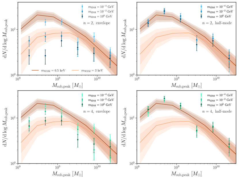
Figure 11: Mean SHMFs, measured using peak virial mass, for our IDM models. ICs for our half-mode (envelope) IDM in the left column (right column) are chosen to match the half-mode wavenumber of (be strictly more suppressed than) the transfer function for $m_{\mathrm{WDM}}=6.5~{}\mathrm{keV}$. The mean SHMF for this WDM model, predicted by our WDM SHMF fit, is shown as a dark orange line in each panel; light orange lines and bands show corresponding results for our $m_{\mathrm{WDM}}=3~{}\mathrm{keV}$ model. For both WDM models, dark (light) bands show $68\%$ ($95\%$) confidence intervals from our fit, calculated by sampling from the posterior.

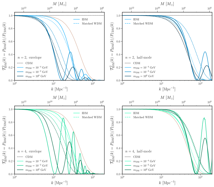
Figure 12: Ratio of the linear matter power spectrum for each IDM model we simulate (solid lines) relative to CDM (dotted black lines), compared to WDM models that produce the same total number of subhalos above the resolution limit (“Matched WDM”, dashed lines). The half-mode IDM models in the left column have the same half-mode scale as the limiting WDM scenario with $m_{\mathrm{WDM}}=6.5~{}\mathrm{keV}$, which is shown as a faint orange line in each panel. The IDM models in the left column are strictly more suppressed than the limiting WDM model.

Figure 11 shows the differential SHMF, as a function of $M_{\mathrm{sub,peak}}$ and subject to our fiducial resolution cut of $M_{\mathrm{sub}}>1.2\times 10^{8}~{}M_{\mathrm{\odot}}$, for each IDM model we simulate. Several results are immediately apparent. First, the envelope IDM models produce SHMFs that are systematically more suppressed than the reference $m_{\mathrm{WDM}}=6.5~{}\mathrm{keV}$ model. This is not surprising, since the corresponding IDM transfer functions were chosen to be strictly more suppressed than this WDM model. Second, many of the envelope IDM models produce total subhalo abundances comparable to the most suppressed WDM model we simulate (i.e., $m_{\mathrm{WDM}}=3~{}\mathrm{keV}$). These results justify the procedure in Maamari et al. (2021) to place bounds on the envelope models using the MW satellite population, as they would produce many fewer satellite galaxies than the limiting $m_{\mathrm{WDM}}=6.5~{}\mathrm{keV}$ WDM model.

The SHMFs in IDM models with the same half-mode scale as $m_{\mathrm{WDM}}=6.5~{}\mathrm{keV}$ are statistically consistent with the SHMFs that best fit the WDM simulations, reported in Section 5.2. As a result, we expect that upper bounds on the IDM cross section from the MW satellite population should be closer to the half-mode than the envelope cross section; this is further quantified below (see Section 6.4). IDM models yield slightly higher subhalo abundances than the $m_{\mathrm{WDM}}=6.5~{}\mathrm{keV}$ model, which indicates that these scenarios are not ruled out at $95\%$ confidence by the Nadler et al. (2021b) analysis, consistent with the reasoning in Maamari et al. (2021).

To facilitate comparisons between IDM and WDM SHMFs, we find the value of $m_{\mathrm{WDM}}$ that yields a total number of subhalos with $M_{\mathrm{sub}}>1.2\times 10^{8}~{}M_{\mathrm{\odot}}$ that most closely matches the value we measure in IDM, after averaging over the three host halos in each scenario. Since our simulation suite only has a limited number of WDM mass benchmarks, to predict the total subhalo abundance as a function of $m_{\mathrm{WDM}}$, we apply the WDM SHMF suppression model from Equation 19, evaluated at the best-fit parameter values from Equation 24, and modify the total count of subhalos measured in the CDM simulations accordingly. We match IDM to WDM based on total subhalo abundance rather than the full SHMF as a simple first-order comparison relevant for limits based on total MW satellite abundances. The results of this procedure are illustrated in Figure 12, and read as follows: for the $n=2$ case ($n=4$), WDM scenarios with particle masses of $7.5$ ($7.6$), $10.4$ ($9.4$), and $6.6$ ($9.7$) keV, match half-mode IDM scenarios with $m_{\mathrm{IDM}}=10^{-4}~{}\mathrm{GeV}$, $10^{-2}~{}\mathrm{GeV}$, and $1~{}\mathrm{GeV}$, respectively; for the $n=4$ case, the same IDM scenarios are matched by WDM scenarios with particle masses of $7.6$, $9.4$, and $9.7$ keV, respectively; for the corresponding envelope models, we obtain $4.1$, $2.7$, and $2.2$ keV for $n=2$, and $4.5$, $3.5$, and $2.8$ keV for $n=4$.

Several interesting comparisons between IDM models emerge from Figure 12. In the half-mode panels, the key takeaway is that all IDM transfer functions yield statistically indistinguishable subhalo abundances, as shown in Figure 11. For example, compare the transfer functions for $m_{\mathrm{IDM}}=10^{-2}~{}\mathrm{GeV}$ and $1~{}\mathrm{GeV}$ half-mode models with $n=4$, which mainly differ in the height of the first DAO peak. The similarity of the resulting subhalo abundances implies that our measurement is not sensitive to the amplitude of the DAO peak for $k_{\mathrm{peak}}\gtrsim 100~{}\mathrm{Mpc}^{-1}$. This wavenumber corresponds to a mass of $\approx 5\times 10^{6}~{}M_{\mathrm{\odot}}$, well below our resolution limit.

DAOs play a more significant role for our envelope models because they appear on the scales of resolved halos. For $n=4$, the $m_{\mathrm{IDM}}=10^{-2}~{}\mathrm{GeV}$ case is matched to a less suppressed WDM transfer function than the $1~{}\mathrm{GeV}$ case, even though its initial cutoff occurs at smaller wavenumbers (compare the medium vs. dark green lines in the bottom-left panel of Figure 12). Thus, SHMF suppression is reduced due to the large DAOs in the $m_{\mathrm{IDM}}=10^{-2}~{}\mathrm{GeV}$ envelope model. A similar result holds for $n=2$ models (compare the medium vs. dark blue lines in the top-left panel of Figure 12). Note that the impact of DAOs varies over the range of IDM masses we study. For example, the $m_{\mathrm{IDM}}=10^{-4}~{}\mathrm{GeV}$ models behave fairly similarly to WDM because of their small DAOs, although minor differences persist even in these cases because of the steeper initial cutoffs in these models.

Several previous studies have simulated IDM models with DAOs, although (to our knowledge) no zoom-in simulations have been performed with ICs for the DM–baryon scattering models we consider. In particular, Schewtschenko et al. (2016) ran simulations with ICs appropriate for DM–photon scattering; DAOs in the models they simulate are small, with typical peak heights of $\mathcal{O}(1\%)$ relative to CDM (also see Boehm et al. 2014; Schewtschenko et al. 2015). These authors find that WDM and DM–photon scattering models with matched $k_{\mathrm{hm}}$ yield similar subhalo populations, consistent with our findings for IDM models with small DAOs (i.e., the $m_{\mathrm{IDM}}=10^{-4}~{}\mathrm{GeV}$ cases for $n=2$ and $n=4$). These results lend confidence to studies that match such models to WDM to derive constraints (e.g., Crumrine et al. 2024).

Other previous studies have simulated models with larger DAOs, comparable to our IDM ICs. For example, Vogelsberger et al. (2016) ran zoom-in simulations of ETHOS models that include both linear matter power spectrum suppression and late-time self-interactions. Because these models feature non-gravitational interactions, we defer a detailed comparison to Paper III of the COZMIC series, in which we consider similar scenarios. Meanwhile, Bohr et al. (2020, 2021) ran cosmological simulations of ETHOS models at $z\gtrsim 5$, parameterized by $k_{\mathrm{peak}}$ and $h_{\mathrm{peak}}$, including cases with $\mathcal{O}(1)$ DAO peaks in the transfer function. That study finds that, at high redshifts, only models with $k_{\mathrm{peak}}\lesssim 70~{}\mathrm{Mpc}^{-1}$ and $h_{\mathrm{peak}}\gtrsim 0.2$ affect the abundance of $\approx 10^{8}~{}M_{\mathrm{\odot}}$ differently than WDM. This picture is qualitatively consistent with our MW subhalo population results at $z=0$, even though we do not directly observe oscillatory features in our mass functions. Thus, models with small DAOs ($h_{\mathrm{peak}}\lesssim 0.2$) are unlikely to be distinguished from WDM using their effects on (sub)halo abundances alone. It will be interesting to test whether (sub)halo density profiles can additionally be used to differentiate these models from each other and from WDM, which we leave for future work.

6 Bounds on beyond-CDM Scenarios

We now apply our new SHMF models from Section 5 to derive updated limits on WDM and FDM, and to estimate updated limits on the IDM cross section, using the MW satellite galaxy population measured by DES and PS1 in Drlica-Wagner et al. (2020).

6.1 Procedure

We use the inference framework from Nadler et al. (2019a, 2020, 2021b), which combines DM–only zoom-in simulations (Mao et al., 2015), an empirical galaxy–halo connection model (Nadler et al., 2018, 2019b, 2020), and DES and PS1 MW satellite population observations and selection functions (Drlica-Wagner et al., 2020) to place constraints on beyond-CDM models. This framework allows us to conservatively marginalize over a wide range of galaxy–halo connection scenarios in order to obtain robust constraints. Following Nadler et al. (2021b), we do not alter the galaxy–halo connection parameterization in our beyond-CDM scenarios. Thus, we assume that satellite abundances are affected in our beyond-CDM scenarios but that the observable properties of existing satellites are not, leaving a study of the potential coupling between our galaxy–halo connection parameterization and beyond-CDM physics to future work (see Nadler et al. 2024 for further discussion).

In detail, we generate satellite population realizations using the eight galaxy–halo connection parameters from Nadler et al. (2021b) plus an additional parameter controlling the SHMF suppression. For WDM and FDM, this parameter is $M_{\mathrm{hm}}$, following our SHMF suppression model (Equation 19); for IDM, we will map to constraints on effective WDM models by matching only the total subhalo abundances. The number of predicted satellites in luminosity and surface brightness bin $i$ in a given realization is

$$n_{\mathrm{pred,}i}=\sum_{s_{i}}p_{\mathrm{detect,}s_{i}}\times(1-p_{\mathrm{disrupt,}s_{i}})\times f_{\mathrm{gal,}s_{i}}\times f_{\mathrm{beyond-CDM},s_{i}},$$ (26)

where $s_{i}$ denotes mock satellites in bin $i$, $p_{\mathrm{detect}}$ is the detection probability determined by the DES and PS1 selection functions (Drlica-Wagner et al., 2020), $p_{\mathrm{disrupt}}$ is the disk disruption probability from Nadler et al. (2018), modified as in Nadler et al. (2020), $f_{\mathrm{gal}}$ is the galaxy occupation fraction modeled following (Nadler et al., 2020), and $f_{\mathrm{beyond-CDM}}$ is the SHMF suppression (Equation 19), which we respectively evaluate at the best-fit parameters for WDM and FDM (Equations 24 and 25, respectively). Thus, we assume that the universal $f_{\mathrm{beyond-CDM}}$ measured across our three hosts applies to the subhalo populations used in Nadler et al. (2021b). In our galaxy–halo connection model, the only subhalo property that $f_{\mathrm{gal}}$ and $f_{\mathrm{beyond-CDM}}$ depend on is $M_{\mathrm{sub,peak}}$; however, these terms suppress satellite abundances with a different dependence on $M_{\mathrm{sub,peak}}$ (Nadler et al., 2024). Meanwhile, $p_{\mathrm{detect}}$ depends on each subhalo’s three-dimensional position, peak $V_{\mathrm{max}}$, and virial radius at accretion, while $p_{\mathrm{disrupt}}$ depends on $V_{\mathrm{max}}$ and mass at accretion, infall scale factor, and distance and scale factor at first pericenter.

The probability of observing $n_{\mathrm{obs,i}}$ satellites in bin $i$ is then (Nadler et al., 2019b, 2020, 2024)

$$P(n_{\mathrm{obs},i}|\bm{\theta}_{\mathrm{g-h}},M_{\mathrm{hm}})$$

$$=\Big{(}\frac{N_{\mathrm{real.}}+1}{N_{\mathrm{real.}}}\Big{)}^{-({N}_{i}+1)}\times(N_{\mathrm{real.}}+1)^{-n_{\mathrm{obs},i}}\frac{\Gamma({N}_{i}+n_{\mathrm{obs},i}+1)}{\Gamma(n_{\mathrm{obs},i}+1)\Gamma({N}_{i}+1)},$$ (27)

where $\bm{\theta}_{\mathrm{g-h}}$ represents the eight galaxy–halo connection parameters from Nadler et al. (2021b); ${N_{\mathrm{real.}}}$ is the number of model realizations at fixed galaxy–halo connection and beyond-CDM parameters; and ${N}_{i}\equiv\sum_{j=1}^{{N_{\mathrm{real.}}}}n_{\mathrm{pred},ij}$. Note that $N_{\mathrm{real.}}$ includes draws over different zoom-ins, different observer locations within each zoom-in (with the on-sky LMC position held fixed), and multiple realizations of the stochastic galaxy–halo connection model for each of these choices; we use $N_{\mathrm{real.}}=10$, following Nadler et al. (2024).

Finally, we calculate the likelihood of observing the DES and PS1 MW satellite population given a galaxy–halo connection and beyond-CDM model (Nadler et al., 2020, 2021b)

$$P(\mathbf{n}_{\mathrm{obs}}\lvert\bm{\theta}_{\mathrm{g-h}},M_{\mathrm{hm}})=\prod_{\mathrm{bins\ }i}P(n_{\mathrm{obs},i}|\bm{\theta}_{\mathrm{g-h}},M_{\mathrm{hm}}),$$ (28)

where $\mathbf{n}_{\mathrm{obs}}$ is a vector of observed satellite counts in luminosity and surface brightness bins over all realizations. We insert this likelihood into Bayes’ theorem to calculate the posterior

$$P(\bm{\theta}_{\mathrm{g-h}},M_{\mathrm{hm}}\lvert\mathbf{n}_{\mathrm{obs}})=\frac{P(\mathbf{n}_{\mathrm{obs}}\lvert\bm{\theta}_{\mathrm{g-h}},M_{\mathrm{hm}})P(\bm{\theta}_{\mathrm{g-h}},M_{\mathrm{hm}})}{P(\mathbf{n}_{\mathrm{obs}})},$$ (29)

where $P(\bm{\theta}_{\mathrm{g-h}},M_{\mathrm{hm}})$ is the galaxy–halo connection and beyond-CDM prior. We use the same galaxy–halo connection priors for all parameters as Nadler et al. (2021b), and we sample $\log(M_{\mathrm{hm}}/M_{\mathrm{\odot}})$ uniformly over the interval $[7,10]$ for both WDM and FDM; this choice is conservative, since the marginalized posterior just begins to plateau at the lower limit of this prior. We sample the posterior by running emcee (Foreman-Mackey et al., 2013) for $\sim 10^{6}$ steps with $36$ walkers, discarding $\sim 10^{5}$ burn-in steps, which yields well-converged posteriors with hundreds of independent samples. Marginalizing over $\bm{\theta}_{\mathrm{g-h}}$ yields the marginalized posterior $P(M_{\mathrm{hm}})$, which we use to derive our constraints.

Note that Nadler et al. (2021b) used two zoom-in simulations from the original Symphony Milky Way suite (Mao et al., 2015). Here, we apply our new beyond-CDM SHMF models to this original pipeline to isolate how the constraints are affected by our new SHMF models. Thus, we assume that other subhalo population characteristics such as the radial distribution are unchanged in the beyond-CDM scenarios we study. In future work, we plan to combine the galaxy–halo connection inference framework with our new simulations to directly evaluate the MW satellite population likelihood and capture such effects.

6.2 Warm Dark Matter

We present the full posterior from our WDM inference in Appendix G. Following Nadler et al. (2021b), we multiply all values of $M_{\mathrm{hm}}$ in the posterior by the ratio of the $2\sigma$ upper limit on the MW mass from Callingham et al. (2019) to the average mass of the two host halos used in the inference (i.e., by $1.8\times 10^{12}~{}M_{\mathrm{\odot}}/1.4\times 10^{12}~{}M_{\mathrm{\odot}}\approx 1.29$). From the marginalized $M_{\mathrm{hm}}$ posterior, we find $M_{\mathrm{hm}}<3.9\times 10^{7}~{}M_{\mathrm{\odot}}$ at $95\%$ confidence, corresponding to

$$m_{\mathrm{WDM}}>5.9~{}\mathrm{keV}\ \mathrm{(95\%\ confidence).}$$ (30)

This constraint is $0.6~{}\mathrm{keV}$ (or $\approx 10\%$) weaker than the $6.5~{}\mathrm{keV}$ limit derived in Nadler et al. (2021b) mainly because of our updated WDM transfer functions and $M_{\mathrm{hm}}(m_{\mathrm{WDM}})$ relation (see Section 2.1). Our new WDM SHMF model also slightly weakens the limit, since our best-fit $f_{\mathrm{WDM}}$ is marginally less suppressed than the Lovell et al. (2014) model used in Nadler et al. (2021b). In addition to using the best-fit WDM SHMF suppression parameters from Equation 24, we tested marginalizing over $\alpha$, $\beta$, and $\gamma$ using our WDM posterior (Figure 7); the uncertainty contributed by these parameters is much smaller than from our galaxy–halo connection, and our $95\%$ confidence constraint is unchanged in this version of the analysis.

We emphasize that our $m_{\mathrm{WDM}}>5.9~{}\mathrm{keV}$ limit should be interpreted using the latest WDM transfer functions (see Section 2.1 and Vogel & Abazajian 2023) and our new SHMF calibration (see Section 5.2), rather than using previous fits from Viel et al. (2005) and Lovell et al. (2014), respectively. The updated transfer function of our ruled-out $5.9~{}\mathrm{keV}$ WDM model is nearly identical to the Viel et al. (2005) transfer function fit for the ruled-out $6.5~{}\mathrm{keV}$ model from Nadler et al. (2021b). Thus, bounds on other models derived by mapping to the ruled-out WDM transfer function are negligibly affected by our updated WDM analysis.

For completeness, we also present updated $n=0$ IDM bounds following the IDM–WDM half-mode matching procedure from Nadler et al. (2019a, 2021b), which is very accurate for these models. We derive $\sigma_{0}<1.3\times 10^{-29}$, $4.5\times 10^{-29}$, and $2.5\times 10^{-28}~{}\mathrm{cm}^{2}$ for $m_{\mathrm{IDM}}=10^{-4}$, $10^{-2}$, and $1~{}\mathrm{GeV}$, respectively. These constraints are comparable to the MW satellite limits from Nadler et al. (2021b) and are weaker than the Lyman-$\alpha$ forest bounds from Rogers et al. (2022) by a factor of $\approx 2$.

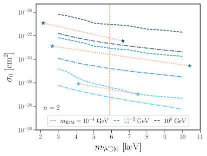
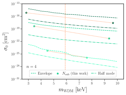
Figure 13: Approximate mapping between the $n=2$ (left) and $n=4$ (right) IDM cross section and $m_{\mathrm{WDM}}$, which we use to estimate updated IDM constraints. In both panels, relations are shown for $m_{\mathrm{IDM}}=10^{-4}$, $10^{-2}$, and $1~{}\mathrm{GeV}$, from lightest to darkest. For each mass, the upper dashed line shows the cross section that yields a $P(k)$ that is strictly more suppressed than WDM models, as a function of $m_{\mathrm{WDM}}$, and the lower dot-dashed line shows cross sections that match the half-mode scales of WDM models. Stars show the effective WDM masses derived by matching to the total abundance of subhalos above the resolution limit in our envelope and half-mode IDM simulations (see Section 5.4). Vertical orange dashed lines show our new $m_{\mathrm{WDM}}=5.9~{}\mathrm{keV}$ limit (Section 6.2); our estimated IDM constraints are derived by linearly interpolating between the star markers in $\log(\sigma_{0}/\mathrm{cm}^{2})$ vs. $m_{\mathrm{WDM}}$, and finding the intersection between the resulting dotted orange lines and the vertical WDM bound.

6.3 Fuzzy Dark Matter

We present the full posterior from our FDM inference in Appendix G, where all values of $M_{\mathrm{hm}}$ are again scaled by the ratio of the observed versus simulated MW host mass. The marginalized posterior yields $M_{\mathrm{hm}}<4.3\times 10^{7}~{}M_{\mathrm{\odot}}$ at $95\%$ confidence, corresponding to

$$m_{\mathrm{FDM}}>1.4\times 10^{-20}~{}\mathrm{eV}\ \mathrm{(95\%\ confidence).}$$ (31)

This constraint is $\approx 5$ times stronger than the $m_{\mathrm{FDM}}>2.9\times 10^{-21}~{}\mathrm{eV}$ limit derived in Nadler et al. (2021b) because our best-fit FDM SHMF suppression is significantly more suppressed than the Schive et al. (2016) model used in Nadler et al. (2021b). We note that our $f_{\mathrm{FDM}}$ model is more similar to (but still more suppressed than) the Du et al. (2018) SHMF fit; Nadler et al. (2021b) derived $m_{\mathrm{FDM}}>9.1\times 10^{-21}~{}\mathrm{eV}$ using this model, which is closer to (but still a factor of $\approx 1.5$ weaker than) our limit. Note that we directly use axionCAMB transfer functions rather than the Hu et al. (2000) fitting function as in Nadler et al. (2021b); however, these yield similar $M_{\mathrm{hm}}(m_{\mathrm{FDM}})$ relations, so this difference does not appreciably affect our FDM limit. As for WDM, marginalizing over the FDM SHMF fit posterior (Figure 9) does not affect our constraint.

Interestingly, the half-mode scales of our ruled-out WDM and FDM models are similar. In the right panel of Figure 10, our simulation with $m_{\mathrm{FDM,22}}=151$ (which has an FDM mass within $10\%$ of our $m_{\mathrm{FDM,22}}$ constraint) reaches a SHMF suppression at $M_{\mathrm{sub,peak}}=10^{8}~{}M_{\mathrm{\odot}}$ that is very similar to our $m_{\mathrm{WDM}}=6~{}\mathrm{keV}$ result, and therefore to our ruled-out $m_{\mathrm{WDM}}=5.9~{}\mathrm{keV}$ model. This follows because the MW satellite constraint is largely driven by suppression near the minimum halo mass of observed satellites, i.e., at $M_{\mathrm{sub,peak}}\approx 10^{8}~{}M_{\mathrm{\odot}}$ (Nadler et al., 2021b).

Our new FDM limit is $\approx 40\%$ weaker than the $2\times 10^{-20}~{}\mathrm{eV}$ Lyman-$\alpha$ forest bound from Rogers & Peiris (2021); this is reasonable given the similar WDM sensitivity of these probes. Meanwhile, our bound is a factor of $\approx 20$ weaker than the $3\times 10^{-19}~{}\mathrm{eV}$ bound from Dalal & Kravtsov (2022) based on stellar heating in the ultra-faint dwarf galaxies Segue 1 and Segue 2, and a factor of $\approx 6$ stronger than the $2.2\times 10^{-21}~{}\mathrm{eV}$ bound from Zimmermann et al. (2024) based on the stellar kinematics of Leo II. It will be interesting to explore the complementarity between these limits in future work, since the suppression of the linear matter power spectrum affects the formation histories and abundances of the same ultra-faint dwarf galaxies used to derive these bounds.

6.4 Interacting Dark Matter

As discussed in Section 5.4, we have not derived a general model for the IDM SHMF suppression due to the varying impact of DAOs over the range of IDM masses and cross sections we simulate. Nonetheless, we mapped our half-mode and envelope models to effective WDM models by matching total subhalo abundances between the models. Here, we use this mapping to estimate upper bounds on the IDM scattering cross section from the MW satellite population. We assume that the total abundance of subhalos above our resolution limit monotonically decreases with increasing cross section, consistent with our simulation results. We will show that the resulting estimated IDM limits significantly improve on the conservative envelope bounds from Maamari et al. (2021). Thus, our results strongly motivate further simulation and modeling work in these scenarios.

Figure 13 illustrates how we estimate IDM bounds for $n=2$ (left panel), $n=4$ (right panel), and for each $m_{\mathrm{IDM}}$. First, for reference, we calculate IDM cross sections with either ($i$) the same half-mode scale as or ($ii$) transfer functions that are strictly more suppressed than WDM models over a grid of $m_{\mathrm{WDM}}$ values. When evaluated at our new $m_{\mathrm{WDM}}=5.9~{}\mathrm{keV}$ bound, the envelope cross sections (dashed lines) are conservatively excluded because their $P(k)$ are strictly more suppressed than the ruled-out WDM model. Meanwhile, models along the lower end of the band (dot-dashed lines) have $P(k)$ that match the half-mode scale of our newly-constrained WDM transfer function. In Section 5.4, we showed that IDM models produce subhalo abundances that are statistically consistent with WDM models with the same half-mode scale, so we cannot exclude them at $95\%$ confidence.

Instead, we linearly interpolate $\log(\sigma_{0}/\mathrm{cm}^{2})$ as a function of $m_{\mathrm{WDM}}$ using the effective WDM masses derived in Section 5.4 by matching total subhalo abundances to our envelope and half-mode IDM simulation results. This yields a third relation (orange dotted lines) that, by construction, is shifted toward lower $\sigma_{0}$ than the envelope cross sections, since subhalo abundances in IDM envelope simulations are suppressed compared to the $m_{\mathrm{WDM}}=6.5~{}\mathrm{keV}$ case. The relation is also shifted toward higher $\sigma_{0}$ than the half-mode cross sections, since subhalo abundances in half mode-matched IDM simulations are enhanced compared to the $m_{\mathrm{WDM}}=6.5~{}\mathrm{keV}$ case. We evaluate this subhalo abundance-matched relation at our new constraint of $m_{\mathrm{WDM}}=5.9~{}\mathrm{keV}$ to estimate updated IDM limits. For $n=2$, this procedure yields $\sigma_{0}<2.9\times 10^{-27}$, $2.6\times 10^{-24}$, and $6.4\times 10^{-23}~{}\mathrm{cm}^{2}$ for $m_{\mathrm{IDM}}=10^{-4}$, $10^{-2}$, and $1~{}\mathrm{GeV}$, respectively. For $n=4$, we find $\sigma_{0}<1.0\times 10^{-25}$, $2.7\times 10^{-20}$, and $5.7\times 10^{-17}~{}\mathrm{cm}^{2}$ for $m_{\mathrm{IDM}}=10^{-4}$, $10^{-2}$, and $1~{}\mathrm{GeV}$, respectively.

These estimated limits improve on the envelope bounds from Maamari et al. (2021) by one order of magnitude, on average, with a maximum improvement for $m_{\mathrm{IDM}}=1~{}\mathrm{GeV}$ and $n=2$ by a factor of $\approx 20$. To derive more rigorous limits, it is necessary to model the SHMF across the entire IDM parameter space, and marginalize over the theoretical uncertainties in this model, including the varying impact of DAOs. This may be achieved by future work that expands and/or emulates our simulation suite.

7 Discussion

We now discuss our results, focusing on our coverage of beyond-CDM ICs (Section 7.1), caveats in our treatment of beyond-CDM physics using N-body simulations (Section 7.2), and areas for future work using the COZMIC simulation pipeline (Section 7.3).

7.1 Coverage of Beyond-CDM Initial Conditions

We have considered three widely-studied beyond-CDM scenarios that imprint a cutoff in the linear matter power spectrum; specifically, the WDM, FDM, and IDM ICs we simulate span a variety of cutoff shapes and secondary characteristics like DAOs (see Figure 1). Nonetheless, studying an even broader range of ICs will be important to facilitate robust $P(k)$ measurements. Here, we highlight directions for future work in this regard.

First, various beyond-CDM scenarios imprint $P(k)$ suppression that qualitatively differs from the sharp cutoffs we simulate. For example, $\mathcal{T}^{2}(k)$ plateaus in scenarios where a sub-component of DM is a non-CDM species; we simulate such fractional beyond-CDM models in Paper II. In future work, it will be interesting to directly simulate fractional WDM, IDM, and FDM models, which are theoretically motivated (e.g., Arvanitaki et al. 2010; Marsh 2011; Farrar 2022; Moore & Slatyer 2024) and can potentially alleviate cosmological tensions on larger scales (e.g., Rubira et al. 2023; He et al. 2023; Rogers et al. 2023; Rogers & Poulin 2023). Meanwhile, models like millicharged DM can suppress power over a range of scales, with a distinctive shape compared to our IDM scenarios (e.g., Driskell et al. 2022). The scenarios listed above are not well captured by generalized transfer function parameterizations (e.g., Murgia et al. 2017), so it will be important to include them in future beyond-CDM simulation efforts.

Second, many beyond-CDM scenarios imprint $P(k)$ enhancement, rather than suppression. For example, enhancement can arise from large-misalignment angle axions (e.g., Arvanitaki et al. 2020), an early period of matter domination (e.g., Erickcek & Sigurdson 2011), and inflationary fluctuations that produce vector DM (e.g., Graham et al. 2016), among many other possibilities (e.g., see Amin & Mirbabayi 2024). Simulating such models can be challenging, particularly if there is appreciable power on scales below the resolution limit that is not fully captured. Thus, careful convergence testing and reassessment of issues like artificial disruption will be needed to robustly treat enhanced scenarios on small scales using our framework.

Finally, we reiterate that we have only considered beyond-CDM physics insofar as it modifies the linear matter power spectrum. Small-scale structure can also be affected by a wide variety of late-time DM physics (e.g., see Bechtol et al. 2022 for an overview). We consider one such scenario in Paper III, which self-consistently combines $P(k)$ suppression with strong, velocity-dependent SIDM.

7.2 Treatment of Beyond-CDM Physics

We have used standard codes for generating cosmological zoom-in ICs and running N-body simulations. While our simulations robustly map linear matter power spectra to DM–only subhalo populations, it is important to discuss how additional physics in each beyond-CDM scenario we consider might affect our simulations, beyond what is captured by $P(k)$ and our N-body simulation technique alone.

Beginning with WDM, we have shown that our N-body simulations yield well-resolved subhalo populations that are negligibly affected by artificial fragmentation. Nonetheless, several studies have simulated WDM (sub)halo populations using alternative simulation codes that better resolve halos near the free-streaming scale and thus avoid this issue more directly. For example, Angulo et al. (2013) simulated a $m_{\mathrm{WDM}}=0.25~{}\mathrm{keV}$ model using the phase-space sheet method, which mitigates artificial fragmentation and allows their analysis to probe halos well below $M_{\mathrm{hm}}$. These authors demonstrate that halo finding is difficult and even ambiguous in this regime. When restricting to reliably-identified halos, Angulo et al. (2013) find a halo mass function suppression that is broadly consistent with extended Press–Schechter (ePS) predictions from Schneider et al. (2012) and Benson et al. (2013), which are in turn consistent with our results. Meanwhile, Stücker et al. (2022) use a hybrid phase-space sheet plus N-body solver, which inherits the benefits of the phase-space sheet method before shell crossing and of traditional N-body solvers afterwards. In general, while phase-space WDM simulations more accurately resolve halos that form on deeply-suppressed scales, our N-body approach is sufficient given the subhalo mass scales and allowed WDM models we consider. Extensions of our analyses to even lower-mass subhalos will thus need to reassess the impact of spurious subhalos and potential halo finder issues.

Another consideration in WDM is the thermal velocity distribution of particles in the ICs. We use the standard version of MUSIC to generate ICs, and thus do not include this effect. Thermal velocities are expected to be fairly small when our simulations are initialized; for example, following Bode et al. (2001), we obtain a root–mean–square thermal velocity of $\mathcal{O}(1)~{}\mathrm{km\ s}^{-1}$ at $z=99$ in $m_{\mathrm{WDM}}=3~{}\mathrm{keV}$ model. This is much smaller than the virial velocities of the subhalos we resolve. Nonetheless, Benson et al. (2013) show that ePS predictions for the WDM halo mass function are systematically more suppressed below $M_{\mathrm{hm}}$ when thermal velocities are included in the semi-analytic model. Since we mainly analyze halos with $M_{\mathrm{sub,peak}}\gtrsim M_{\mathrm{hm}}$ due to our resolution threshold and choice of WDM models, we do not expect thermal velocities to significantly affect our $f_{\mathrm{WDM}}$ measurements. However, higher-resolution simulations that resolve lower-mass (sub)halos will need to revisit this assumption.

Next, for FDM, we have performed N-body simulations that capture $P(k)$ suppression but do not model the wave dynamics of ultra-light particles. Various cosmological simulation codes have been developed for this purpose, including SPH solvers of the Madelung equations (e.g., Nori & Baldi 2018; Nori et al. 2023; Elgamal et al. 2023) and pseudospectral solvers of the Schrödinger–Poisson equation (e.g., Schive et al. 2014; May & Springel 2021, 2023; Schwabe et al. 2020; Schwabe & Niemeyer 2022). These studies have not found significant differences between the (sub)halo mass function with or without FDM dynamics implemented. For example, May & Springel (2023) show that halo mass function suppression primarily depends on FDM ICs, rather than wave dynamics. In turn, their results are in reasonable agreement with the halo mass function fit from Schive et al. (2016), which was derived using FDM ICs but N-body dynamics. However, semi-analytic models like Du et al. (2018) find differences between the stripping of subhalo profiles with or without solitonic cores. For the relatively large values of $m_{\mathrm{FDM,22}}$ we consider, the impact of FDM wave dynamics on subhalos abundances above our resolution limit is expected to be small, but warrants dedicated analysis in future work.

Lastly, for IDM, we expect our N-body simulations to accurately capture subhalo abundances because the DM–baryon scattering rate drops rapidly with decreasing redshift in the models we consider; indeed, kinetic and thermal decoupling between the DM and baryon fluids typically occur at $z\gtrsim 10^{5}$, well before we initialize our simulations (e.g., Nadler et al. 2019a; Maamari et al. 2021). Nonetheless, DM–baryon scattering may be enhanced in high-density environments at late times, leading to a variety of novel signatures in galaxy and (sub)halo density profiles (e.g., Acevedo et al. 2023, and see Heston et al. 2024 for an example in the context of DM–neutrino scattering). Thus, it will be interesting to explore the potential impact of IDM scattering on subhalo populations as these modeling efforts develop.

7.3 Future Work

We anticipate the following key areas for future work related to COZMIC. First, we have only simulated three independent MW systems: two MW analogs from the Milky Way-est suite (Buch et al., 2024), and one MW–mass host from the Symphony Milky Way suite (Nadler et al., 2023). For WDM and FDM, our derived SHMF suppression parameters are nearly identical among these three hosts; it will be important to critically assess and understand this universality in future work (see Appendix E). In addition, expanding COZMIC to include a larger sample of MW analogs would enable more robust forward-modeling of the MW subhalo and satellite population. For example, we currently marginalize over the MW host halo mass using a conservative analytic approach to derive constraints; however, including more MW realizations in the inference would achieve this marginalization directly. Simulating a larger host sample would also allow us to quantify the potential environmental dependence of SHMF suppression, which we plan to explore in future work.

Second, our analysis is limited to subhalos at $z=0$. The zoom-in region surrounding each host extends several $\mathrm{Mpc}$ from the MW’s center, and a large number of (sub)halos are resolved with high-resolution particles in this region (see Appendix B). To fully exploit our simulations, contamination and convergence studies of (sub)halos throughout the zoom-in regions should be conducted in our beyond-CDM realizations. Meanwhile, many halos are sufficiently resolved in our simulations as early as $z\approx 10$. Thus, our simulations can be used to quantify the redshift dependence of (sub)halo mass function suppression in beyond-CDM scenarios, which we leave to a future study.

Third, we have used the standard halo finder and merger tree codes Rockstar and consistent-trees to post-process our results (see Section 3.3). We expect that implementing particle-tracking codes like Symfind (Mansfield et al., 2024) will yield even more robust subhalo catalogs, particularly for highly-stripped objects, and we plan to apply such tools to COZMIC in future work. More generally, it will be important to revisit halo finder and merger tree code comparisons (e.g., Onions et al. 2012; Srisawat et al. 2013) in beyond-CDM scenarios, since most post-processing codes are calibrated to CDM simulations. For example, the (artificial) disruption of subhalos may differ for objects that form from suppressed linear matter power spectra due to their delayed growth and reduced concentrations. This is an important issue for future work, and particularly for analyses of subhalo density profiles in our beyond-CDM simulations.

Fourth, we have quantified SHMF suppression using DM–only simulations. Baryons are expected to reduce the SHMF in MW–mass hosts relative to CDM via enhanced tidal stripping by the galactic disk (e.g., Garrison-Kimmel et al. 2017; Kelley et al. 2019; Webb & Bovy 2020; Wang et al. 2024). This effect may be enhanced due to the reduced concentrations of subhalos in our beyond-CDM scenarios (Du et al., 2024); (sub)halos with masses $\gtrsim 10^{10}~{}M_{\mathrm{\odot}}$, which host galaxies with stellar masses $\gtrsim 10^{6}~{}M_{\mathrm{\odot}}$ (Nadler et al., 2020), can also develop cores due to repeated episodes of supernova feedback (e.g., Pontzen & Governato 2012; Dutton et al. 2020). Quantifying the correlated impact of baryons and beyond-CDM physics on subhalo populations is therefore an exciting area for future work. This could be achieved by embedding disk potentials in our beyond-CDM simulations, or by performing full hydrodynamic resimulations of our hosts (e.g., similar to Forouhar Moreno et al. 2022).

Finally, by combining the simulations presented here with simulations of additional models in upcoming COZMIC papers, we aim to develop a general (sub)halo mass function model applicable to a broad range of beyond-CDM ICs. For the beyond-CDM scenarios in this paper, one key question is whether our SHMF fitting functions can be extended below the resolution limit, and/or to $M_{\mathrm{hm}}/M_{\mathrm{sub,peak}}$ ratios outside those covered by our simulations, or if they are only accurate in the range of beyond-CDM parameters and subhalo masses covered here. We plan to test this using semi-analytic models and additional simulations. A general SHMF model will ultimately help enable model-independent $P(k)$ reconstruction using small-scale structure data.

8 Conclusions

As the first installment of the COZMIC simulation suite, we have presented $72$ cosmological DM–only zoom-in simulations of two MW–like hosts and one MW–mass host in three beyond-CDM scenarios that suppress the linear matter power spectrum: thermal-relic WDM, ultra-light FDM, and DM–baryon scattering IDM (see Figure 1). To isolate the impact of ICs, we have assumed that these scenarios only impact $P(k)$ and subsequently evolve like CDM. Our work substantially expands the available sample of zoom-in simulations in beyond-CDM cosmologies, and reveals that beyond-CDM SHMF suppression is fairly universal. Two companion studies will expand COZMIC: beyond-CDM simulations with a plateau in the transfer function, characteristic of fractional beyond-CDM models (Paper II; R. An et al., in preparation), and simulations of SIDM models with self-consistently modeled $P(k)$ suppression (Paper III; E. O. Nadler et al., in preparation).

Our main findings are as follows:

1. The SHMF is significantly suppressed in many of our beyond-CDM simulations. The amount of suppression depends on the wavenumber of the $P(k)$ cutoff, and scales differently with microphysical DM parameters in WDM, FDM, and IDM scenarios (Figure 5).

2. The normalized subhalo radial distribution is slightly more concentrated in our beyond-CDM simulations relative to CDM due to the lack of recently-accreted low-mass subhalos; however, this effect is comparable to the host-to-host scatter in radial distributions among our three simulated hosts (Figure 6).

3. We derive a model for WDM SHMF suppression consistent with previous work, with best-fit parameters for Equation 19 given by Equation 24 (see Figure 8).

4. We derive a model for the FDM SHMF suppression that is significantly steeper than WDM and more suppressed than previous work, with best-fit parameters for Equation 19 given by Equation 25, thus reflecting the sharper $P(k)$ cutoff in FDM (see Figure 10).

5. IDM SHMF suppression can be reduced due to dark acoustic oscillations in $P(k)$; the size of this effect varies over the range of IDM cross sections, masses, and velocity dependences we simulate (Figure 12).

6. We derive $m_{\mathrm{WDM}}>5.9~{}\mathrm{keV}$ at $95\%$ confidence from the MW satellite population using our new WDM SHMF suppression model; our result is $\approx 10\%$ weaker than a previous bound using the same framework due to our updated $M_{\mathrm{hm}}(m_{\mathrm{WDM}})$ relation (Equation 6).

7. We derive $m_{\mathrm{FDM}}>1.4\times 10^{-20}$ at $95\%$ confidence from the MW satellite population using our new FDM SHMF suppression model; this constraint is $\approx 5$ times stronger than a previous limit using the same framework because our FDM SHMFs are more suppressed than previous work.

8. We estimate updated MW satellite population bounds on the DM–proton scattering cross section, with an $n=2$ ($n=4$) power-law velocity-dependence, of $\sigma_{0}<2.9\times 10^{-27}$, $2.6\times 10^{-24}$, and $6.4\times 10^{-23}~{}\mathrm{cm}^{2}$ ($\sigma_{0}<1.0\times 10^{-25}$, $2.7\times 10^{-20}$, and $5.7\times 10^{-17}~{}\mathrm{cm}^{2}$) for IDM masses of $10^{-4}$, $10^{-2}$, and $1~{}\mathrm{GeV}$, respectively. These estimates are derived using an approximate mapping to total WDM subhalo abundances. The results motivate a future study leveraging a larger set of IDM simulations and the development of IDM SHMF models, which have the potential to improve IDM cross section bounds by up to a factor of $\sim 20$ with current data.

Upcoming galaxy surveys will critically test our beyond-CDM predictions. For example, the Rubin Observatory Legacy Survey of Space and Time (LSST; Ivezić et al. 2008) is expected to discover most of the remaining MW satellite population in the Southern hemisphere (e.g., Drlica-Wagner et al. 2019; K. Tsiane et al., in preparation). Combining this data with our beyond-CDM SHMF predictions and galaxy–halo connection framework will simultaneously advance our understanding of galaxy formation and DM physics; for example, see the forecasts in Nadler et al. (2024).

In parallel, upcoming data from the Nancy Grace Roman Space Telescope (Spergel et al., 2015; Gezari et al., 2022) and other upcoming observational facilities (Chakrabarti et al., 2022) will provide complementary information about small-scale structure, both within the MW (e.g., by characterizing its stellar stream population) and beyond (e.g., by discovering new strong gravitational lens systems). We expect COZMIC to inform modeling efforts for all of these science targets. These same facilities will advance measurements of small-scale structure using strong gravitational lensing and stellar streams, which probe the beyond-CDM models we consider through their effects on both (sub)halo abundances and density profiles (e.g., see Vegetti et al. 2023 and Bonaca & Price-Whelan 2024 for reviews). It is therefore timely to expand our suite to higher-mass hosts relevant for strong lensing (e.g., using the Symphony Group suite from Nadler et al. 2023), and to use it as a template for modeling the low-mass subhalos in the inner MW that perturb stellar streams.

Looking forward, the development of small-scale structure emulators in beyond-CDM scenarios is well motivated, following recent efforts using hydrodynamic simulations of MW–mass systems (e.g., Brown et al. 2024; Rose et al. 2024). The advantage of our N-body approach is its relatively low computational cost, which allows us to simulate a wide range of beyond-CDM models. COZMIC thus facilitates predictions for the MW subhalo and satellite galaxy population across a wide range of possible linear matter power spectra. This effort will ultimately enable robust, model-independent reconstruction of the small-scale linear matter power spectrum using near-field cosmological observables.

Appendix A Transfer Function Calculations

A.1 Warm Dark Matter

In our WDM CLASS runs, we consider a thermal relic particle with a Fermi-Dirac phase-space distribution characterized by the WDM-to-photon temperature ratio (Colombi et al., 1996),

$$\frac{T_{\mathrm{WDM}}}{T_{\gamma}}=\Omega_{\mathrm{WDM}}h^{2}\left(\frac{4}{11}\right)^{1/3}\left(\frac{m_{\mathrm{WDM}}}{94\ \mathrm{eV}}\right)^{-1},$$ (A1)

where $\Omega_{\mathrm{WDM}}$ is the present-day fractional WDM density, which corresponds to the entire DM density in our WDM simulations, i.e., $\Omega_{\mathrm{WDM}}=\Omega_{\rm m}$. We have compared the resulting transfer functions to the Decant et al. (2022) and Vogel & Abazajian (2023) fitting functions for $\mathcal{T}^{2}_{\mathrm{WDM}}(k)$, finding that they both match our CLASS output very well.

Rather than using a fitting function for $\mathcal{T}^{2}_{\mathrm{WDM}}(k)$ to generate ICs, as done in many previous WDM simulations, we directly use CLASS transfer functions as input for MUSIC to ensure accurate ICs. The current version of MUSIC only features a CAMB transfer function plug-in. Thus, we convert CLASS density transfer functions into CAMB format by setting format = camb; we also convert CLASS Newtonian-gauge velocity transfer functions, $\theta$, to velocity transfer functions in CAMB format, $\mathcal{T}_{v}$, via

$$\mathcal{T}_{v,i}=\theta_{i}/(\tilde{H}\tilde{k}^{2}).$$ (A2)

Here, $i$ represents the particle species (DM or baryons), $\tilde{H}$ is the Hubble parameter in units of $\mathrm{Mpc}^{-1}$ at the initial redshift ($z=99$), and $\tilde{k}$ is the comoving wavenumber in units of $\mathrm{Mpc}^{-1}$.

A.2 Fuzzy Dark Matter

We make the following minor modifications to version v1.0 of axionCAMB. By default, the velocity transfer function of FDM is not output by axionCAMB; we therefore modify the code to output this transfer function in the same format as for CDM. Furthermore, for $k\gg k_{J}$, the linear FDM density perturbation $\delta(k)$ oscillates with time instead of growing as in CDM, which can lead to negative values in the transfer functions. To avoid numerical errors, we therefore take the absolute values of these transfer functions before implementing them in MUSIC. This procedure does not affect our results, as the negative values only occur on extremely small scales. A patch with our changes to axionCAMB is available at https://github.com/Xiaolong-Du/axionCAMB_patch.

A.3 Interacting Dark Matter

To generate IDM transfer functions, we input $m_{\mathrm{IDM}}$, $\sigma_{0}$, and $n$ into our modified CLASS code. We then convert the transfer functions to CAMB format using the method described above for WDM. Note that the resulting half-mode and envelope IDM cross sections are slightly different than derived in Maamari et al. (2021) because we match to an updated $m_{\mathrm{WDM}}=6.5~{}\mathrm{keV}$ transfer function.

Appendix B Table of Simulation Results

Table 2 summarizes the main properties of the host halo, subhalo population, and isolated halo population in each of our fiducial-resolution beyond-CDM simulations.

Table 2: Properties of Our Standard Resolution Beyond-CDM Simulations

Scenario	Input Parameter(s)	Halo004	Halo113	Halo023
	–	$M_{\mathrm{host,12}},\ c_{\mathrm{host}},\ N_{\mathrm{sub}},\ N_{\mathrm{iso}}$	$M_{\mathrm{host,12}},\ c_{\mathrm{host}},\ N_{\mathrm{sub}},\ N_{\mathrm{iso}}$	$M_{\mathrm{host,12}},\ c_{\mathrm{host}},\ N_{\mathrm{sub}},\ N_{\mathrm{iso}}$
CDM	–	1.03, 10.8, 93, 630	1.07, 10.6, 77, 882	1.14, 11.5, 69, 761
	$m_{\mathrm{WDM}}~{}[\mathrm{keV}]$	$M_{\mathrm{host,12}},\ c_{\mathrm{host}},\ N_{\mathrm{sub}},\ N_{\mathrm{iso}}$	$M_{\mathrm{host,12}},\ c_{\mathrm{host}},\ N_{\mathrm{sub}},\ N_{\mathrm{iso}}$	$M_{\mathrm{host,12}},\ c_{\mathrm{host}},\ N_{\mathrm{sub}},\ N_{\mathrm{iso}}$
	3	1.03, 10.6, 40, 224	1.07, 10.6, 33, 334	1.17, 10.7, 38, 265
	4	1.04, 10.4, 57, 346	1.06, 10.4, 44, 488	1.11, 12.5, 45, 420
Thermal-relic	5	1.04, 10.4, 66, 431	1.06, 10.8, 58, 594	1.12, 12.4, 57, 519
WDM	6	1.03, 10.7, 79, 490	1.06, 10.9, 66, 674	1.11, 12.2, 64, 596
	6.5	1.03, 10.4, 79, 518	1.06, 10.9, 65, 709	1.14, 11.7, 59, 629
	10	1.03, 10.3, 90, 583	1.06, 11.0, 76, 814	1.14, 11.4, 61, 714
	$m_{\mathrm{FDM}}~{}[10^{-22}~{}\mathrm{eV}]$	$M_{\mathrm{host,12}},\ c_{\mathrm{host}},\ N_{\mathrm{sub}},\ N_{\mathrm{iso}}$	$M_{\mathrm{host,12}},\ c_{\mathrm{host}},\ N_{\mathrm{sub}},\ N_{\mathrm{iso}}$	$M_{\mathrm{host,12}},\ c_{\mathrm{host}},\ N_{\mathrm{sub}},\ N_{\mathrm{iso}}$ .
	25.9	1.04, 12.4, 36, 213	1.07, 10.4, 31, 308	1.16, 11.7, 37, 257
	69.4	1.04, 11.1, 68, 419	1.08, 9.8, 60, 560	1.12, 12.2, 54, 495
Ultra-light	113	1.04, 10.2, 82, 506	1.08, 10.4, 72, 687	1.11, 12.5, 64, 617
FDM	151	1.04, 10.1, 89, 545	1.07, 10.6, 74, 748	1.11, 12.2, 69, 664
	185	1.03, 10.1, 95, 576	1.07, 10.7, 76, 792	1.14, 11.6, 71, 698
	490	1.03, 10.6, 97, 612	1.07, 10.7, 84, 852	1.13, 11.7, 71, 756
	$m_{\mathrm{IDM}}~{}[\mathrm{GeV}]$, $\sigma_{0}~{}[\mathrm{cm}^{2}]$	$M_{\mathrm{host,12}},\ c_{\mathrm{host}},\ N_{\mathrm{sub}},\ N_{\mathrm{iso}}$	$M_{\mathrm{host,12}},\ c_{\mathrm{host}},\ N_{\mathrm{sub}},\ N_{\mathrm{iso}}$	$M_{\mathrm{host,12}},\ c_{\mathrm{host}},\ N_{\mathrm{sub}},\ N_{\mathrm{iso}}$ .
	$10^{-4}$, $4.2\times 10^{-28}$	1.03, 10.3, 84, 544	1.07, 10.7, 74, 744	1.14, 11.7, 60, 659
	$10^{-4}$, $2.8\times 10^{-27}$	1.03, 11.1, 60, 348	1.07, 10.1, 52, 486	1.16, 11.3, 44, 414
DM–proton scattering	$10^{-2}$, $1.3\times 10^{-25}$	1.03, 10.2, 86, 549	1.07, 10.5, 77, 749	1.14, 11.7, 68, 678
IDM ($n=2$)	$10^{-2}$, $7.1\times 10^{-24}$	1.03, 10.8, 37, 238	1.06, 11.1, 19, 345	1.14, 11.9, 34, 269
	$1$, $1.6\times 10^{-23}$	1.03, 9.9, 84, 538	1.07, 10.8, 69, 737	1.14, 11.7, 57, 658
	$1$, $8.0\times 10^{-22}$	1.03, 9.8, 27, 168	1.06, 11.0, 12, 262	1.13, 11.2, 24, 216
	$m_{\mathrm{IDM}}~{}[\mathrm{GeV}]$, $\sigma_{0}~{}[\mathrm{cm}^{2}]$	$M_{\mathrm{host,12}},\ c_{\mathrm{host}},\ N_{\mathrm{sub}},\ N_{\mathrm{iso}}$	$M_{\mathrm{host,12}},\ c_{\mathrm{host}},\ N_{\mathrm{sub}},\ N_{\mathrm{iso}}$	$M_{\mathrm{host,12}},\ c_{\mathrm{host}},\ N_{\mathrm{sub}},\ N_{\mathrm{iso}}$ .
	$10^{-4}$, $2.2\times 10^{-27}$	1.03, 10.3, 82, 536	1.07, 10.9, 74, 735	1.14, 11.5, 63, 642
	$10^{-4}$, $3.4\times 10^{-26}$	1.04, 10.9, 63, 376	1.08, 10.2, 59, 516	1.14, 11.5, 46, 462
DM–proton scattering	$10^{-2}$, $1.7\times 10^{-22}$	1.03, 9.8, 85, 564	1.08, 10.5, 80, 771	1.13, 11.6, 63, 695
IDM ($n=4$)	$10^{-2}$, $1.7\times 10^{-19}$	1.02, 12.7, 53, 373	1.06, 9.8, 32, 490	1.15, 11.1, 44, 418
	$1$, $8.6\times 10^{-19}$	1.03, 10.1, 83, 557	1.08, 10.6, 80, 758	1.14, 11.5, 66, 680
	$1$, $2.8\times 10^{-16}$	1.04, 12.2, 42, 238	1.07, 10.3, 22, 357	1.14, 11.7, 35, 308

Note. — The first column lists the name of each DM scenario we consider, the second column lists input parameter(s) used to generate ICs for our simulations, and the third, fourth, and fifth columns respectively list simulation results for our MW–like hosts, Halo004 and Halo113, and our MW–mass host, Halo023. We list the host halo virial mass, $M_{\mathrm{host,12}}\equiv M_{\mathrm{host}}/10^{12}~{}M_{\mathrm{\odot}}$, and virial concentration, $c_{\mathrm{host}}\equiv R_{\mathrm{vir,host}}/R_{s\mathrm{,host}}$ (where $R_{s}$ is the NFW scale radius), along with the total number of subhalos within the MW host’s virial radius ($N_{\mathrm{sub}}$) and isolated halos within $3~{}\mathrm{Mpc}$ of the MW host’s center ($N_{\mathrm{iso}}$) above our fiducial resolution threshold of $M_{\mathrm{sub}}>1.2\times 10^{8}~{}M_{\mathrm{\odot}}$. For each IDM mass, the first (second) row corresponds to our half-mode (envelope) models.

Appendix C Convergence Tests

To test that our key results are converged, we run high-resolution (HR) resimulations in CDM and all beyond-CDM models for Halo004, for a total of 25 resimulations. These runs use five MUSIC refinement regions, i.e., an equivalent of $16384$ particles per side in the highest-resolution regions, and a particle mass of $m_{\mathrm{part,HR}}=5.0\times 10^{4}~{}M_{\mathrm{\odot}}$. We set the comoving Plummer-equivalent gravitational softening to $\epsilon_{\mathrm{HR}}=80~{}\mathrm{pc}~{}h^{-1}$, following Nadler et al. (2023).

The results of our convergence tests are in good agreement with Symphony and Milky Way-est CDM results (Nadler et al., 2023; Buch et al., 2024). Specifically, in both CDM and all beyond-CDM models we simulate, the present-day SHMF is converged at the $\approx 10\%$ level down to our fiducial $M_{\mathrm{sub}}>1.2\times 10^{8}~{}M_{\mathrm{\odot}}$ ($300$-particle) threshold. In the absence of an $M_{\mathrm{sub}}$ resolution cut, the $M_{\mathrm{sub,peak}}$ only reaches this level of convergence above an $M_{\mathrm{sub,peak}}\gtrsim 4\times 10^{8}~{}M_{\mathrm{\odot}}$ ($1000$-particle) threshold due to subhalos that are stripped below the present-day mass resolution limit (see the discussion in Nadler et al. 2023). However, our main results concern the suppression of the peak SHMF subject to an $M_{\mathrm{sub}}$ cut, and we find that this quantity is better converged both in CDM and across our beyond-CDM models.

Quantitatively, Figure 14 shows the ratio of the peak SHMF suppression in our standard versus HR simulations; we do not find systematic differences in the behavior of this ratio across our beyond-CDM models, so we combine all beyond-CDM models in this figure. Our measurement of $f_{\mathrm{beyond-CDM}}$ is converged at the $\approx 10\%$ level for the lowest-mass subhalos we resolve in our fiducial-resolution simulations, given both the statistical uncertainty and model-to-model scatter. Thus, our SHMF suppression fits, which are driven by the lowest-mass subhalos we resolve, are well converged. We further verify this by re-fitting our WDM and FDM SHMF models to the HR simulations alone; the resulting posteriors are consistent with our fiducial results. Subhalo radial distributions are more variable between resolution levels, similar to the results in Nadler et al. (2023), which may reflect stochasticity in subhalo orbits and/or slower convergence of the radial distribution. Nonetheless, inner normalized radial distributions remain more concentrated than CDM in our beyond-CDM HR simulations, supporting our findings in Section 4.3.

The tests above are necessary (but not sufficient) to demonstrate convergence to a physical solution. For example, Mansfield et al. (2024) use a particle tracking method to that Rockstar and consistent-trees (the tools we use in this study) identify too few subhalos in Symphony CDM simulations, particularly for highly-stripped systems in hosts’ inner regions. We leave a particle-tracking analysis of COZMIC simulations to future work.

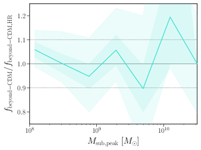
Figure 14: Ratio of the differential beyond-CDM peak SHMF relative to CDM, for subhalos with $M_{\mathrm{sub}}>1.2\times 10^{8}~{}M_{\mathrm{\odot}}$ in our fiducial-resolution simulations of Halo004, relative to the same quantity in our HR resimulations of the same host. The bold line shows the mean ratio stacked across all $24$ beyond-CDM models; dark (light) bands show $1\sigma$ Poisson uncertainty (model-to-model scatter).

Appendix D Artificial Fragmentation

Previous analyses of beyond-CDM simulations have derived a resolution-dependent mass limit, $M_{\mathrm{lim}}$ below which a significant fraction of subhalos are formed spuriously, i.e., through artificial fragmentation. Specifically, they define the characteristic mass (Wang & White, 2007)

$$M_{\mathrm{lim}}=10.1\bar{\rho}dk_{\mathrm{peak}}^{-2},$$ (D1)

where $\bar{\rho}$ is the average matter density, $d$ is the mean interparticle spacing ($22~{}\mathrm{kpc}$ for our fiducial-resolution simulations; Nadler et al. 2023), and $k_{\mathrm{peak}}$ is the wavenumber at which the dimensionless linear matter power spectrum, $\Delta^{2}(k)\equiv k^{3}P(k)/2\pi$, is maximized. Lovell et al. (2014) find that spurious subhalos significantly contribute to the total population at masses below $\kappa M_{\mathrm{lim}}$, where $\kappa\approx 0.5$.

For each beyond-CDM model, we obtain $k_{\mathrm{peak}}$ from our CLASS or axionCAMB output. Plugging these into Equation D1 yields $M_{\mathrm{lim}}=[0.53,0.34,0.21,0.13,0.11,0.05]\times 10^{8}~{}M_{\mathrm{\odot}}$ for $m_{\mathrm{WDM}}=[3,4,5,6,6.5,10]~{}\mathrm{keV}$, $M_{\mathrm{lim}}=[0.31,0.13,0.09,0.07,0.05,0.02]\times 10^{8}~{}M_{\mathrm{\odot}}$ for $m_{\mathrm{FDM,22}}=[25.9,69.4,113,151,185,490]$, $M_{\mathrm{lim}}=[0.25,1.41,1.49]\times 10^{8}~{}M_{\mathrm{\odot}}$ ($[0.08,0.07,0.08]\times 10^{8}~{}M_{\mathrm{\odot}}$) for our $n=2$ envelope (half-mode) models with $m_{\mathrm{IDM}}=10^{-4}$, $10^{-2}$, and $1~{}\mathrm{GeV}$, and $M_{\mathrm{lim}}=[0.20,0.13,1.48]\times 10^{8}~{}M_{\mathrm{\odot}}$ ($[0.09,0.003,0.07]\times 10^{8}~{}M_{\mathrm{\odot}}$) for our $n=4$ envelope (half-mode) models with $m_{\mathrm{IDM}}=10^{-4}$, $10^{-2}$, and $1~{}\mathrm{GeV}$. Thus, as described in Section 3.3, $\kappa M_{\mathrm{lim}}<M_{\mathrm{res}}=1.2\times 10^{8}~{}M_{\mathrm{\odot}}$ for all of our simulations; moreover, our only simulations with $M_{\mathrm{lim}}\gtrsim 10^{8}~{}M_{\mathrm{\odot}}$ are a subset of our envelope IDM runs.

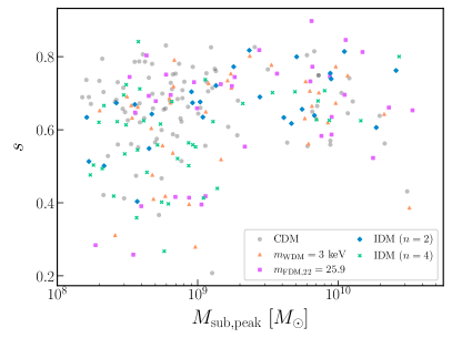
Figure 15: Protohalo sphericity versus peak virial mass for each subhalo with $M_{\mathrm{sub}}>1.2\times 10^{8}~{}M_{\mathrm{\odot}}$ in our CDM simulation of Halo004 (gray circles), compared to the same halo simulated with initials conditions for $m_{\mathrm{WDM}}=3~{}\mathrm{keV}$ (orange triangles), $m_{\mathrm{FDM,22}}=25.9$ (magenta squares), and $m_{\mathrm{IDM}}=1~{}\mathrm{GeV}$ envelope models with $n=2$ (blue diamonds) and $n=4$ (green crosses). Note that these models provide an upper limit on the spurious halo contribution in each beyond-CDM scenario we consider; thus, spurious halos contribute negligibly to our results.

To more directly demonstrate that spurious halos do not impact our results, we study Halo004 simulations with the largest $M_{\mathrm{lim}}$ in each beyond-CDM scenario: $m_{\mathrm{WDM}}=3~{}\mathrm{keV}$, $m_{\mathrm{FDM,22}}=25.9$, and $n=2$ and $n=4$ envelope IDM models with $m_{\mathrm{IDM}}=1~{}\mathrm{GeV}$; these cases provide upper limits on the spurious halo contribution in each scenario. Following Lovell et al. (2014), we identify main-branch progenitors of present-day subhalos with $M_{\mathrm{sub}}>1.2\times 10^{8}~{}M_{\mathrm{\odot}}$ in each of these simulations. We select each progenitor at the redshift, $z_{1/2}$, when its mass first reaches $0.5M_{\mathrm{sub,peak}}$ before infall into any larger halo. We then find all high-resolution particles within each progenitor’s virial radius at $z_{1/2}$ and identify a protohalo by tracing those particles back to the ICs. For each protohalo in the ICs, we calculate the inertia tensor

$$I_{ij}=\sum_{\mathrm{protohalo\ particles}}m_{\mathrm{part}}\left(\delta_{ij}\lvert\mathbf{x}\rvert^{2}-x_{i}x_{j}\right),$$ (D2)

where $\delta_{ij}$ is the Kronecker delta and $x_{i}$ are position vector components. We calculate the eigenvalues $a\geq b\geq c$ of this tensor and define the sphericity

$$s\equiv c/a.$$ (D3)

Note that all of our sphericity measurements are performed using at least $150$ particles, since we only consider subhalos with $M_{\mathrm{sub,peak}}\geq M_{\mathrm{sub}}(z=0)>M_{\mathrm{res}}=300m_{\mathrm{part}}$ and then identify their progenitors at $z_{1/2}$.

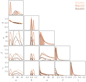
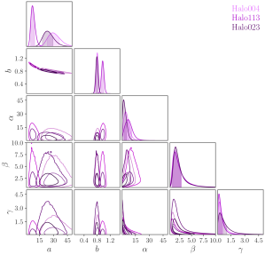
Figure 16: Marginalized posterior for our WDM (left) and FDM (right) SHMF model fit to Halo004, Halo113, and Halo023, from lightest to darkest colors. Dark (light) two-dimensional contours show $68\%$ ($95\%$) confidence intervals; top and side panels show marginal posteriors with shaded $68\%$ confidence intervals.

Lovell et al. (2014) find that $99\%$ of their CDM protohalos have sphericities $s>0.16$; the average sphericity of their CDM protohalo sample is $\langle s\rangle\approx 0.4$. These authors thus use $s>0.16$ as a threshold to remove spurious halos. Our CDM subhalos with $M_{\mathrm{sub}}>1.2\times 10^{8}~{}M_{\mathrm{\odot}}$ have similarly high sphericities in the ICs, with a minimum of $s_{\mathrm{min}}=0.21$ and an average of $\langle s\rangle\approx 0.66$ for the corresponding protohalos. Figure 15 shows that the sphericity distributions of resolved subhalos in our most extreme beyond-CDM simulations are very similar to CDM. In particular, we find $s_{\mathrm{min}}=[0.28,0.26,0.40,0.27]$ and $\langle s\rangle\approx[0.62,0.64,0.67,0.59]$ for protohalos in $m_{\mathrm{wdm}}=3~{}\mathrm{keV}$, $m_{\mathrm{FDM,22}}=25.9$, and $n=2$ and $n=4$ envelope IDM models with $m_{\mathrm{IDM}}=1~{}\mathrm{GeV}$, respectively.

Thus, even in our most extreme beyond-CDM simulations, the subhalos we analyze form from particle distributions with quantitatively similar shapes compared to CDM. This result implies that spurious halos contribute negligibly to our results. Furthermore, we show in Appendix F that the formation time distribution of subhalos in our beyond-CDM subhalos is a smooth function of parameters like $m_{\mathrm{WDM}}$, which can be violated if a significant fraction of subhalos form spuriously (e.g., Bose et al. 2016).

Appendix E Host-to-host Variation in Subhalo Mass Function and Suppression Parameters

To derive our SHMF suppression results in Section 5, we simultaneously fit our SHMF model in Equation 18 to all three hosts we simulate. This model has independent normalizations ($a_{i}$) and slopes ($b_{i}$) for the three hosts, but shared suppression parameters ($\alpha$, $\beta$, and $\gamma$). Here, we show that fitting our MW–like (Halo004 and Halo113) and MW–mass (Halo023) hosts individually yields consistent results for the WDM and FDM SHMF suppression parameters, and we compare the derived normalizations and slopes.

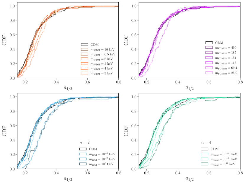
Figure 17: Normalized cumulative distributions of half-mass scale factor—defined by $M_{\mathrm{sub}}(a_{1/2})\equiv 0.5\times M_{\mathrm{sub}}(a=1)$—for subhalos with $M_{\mathrm{sub}}>1.2\times 10^{8}~{}M_{\mathrm{\odot}}$ in our WDM (top left), FDM (top right), and $n=2$ (bottom left) and $n=4$ (bottom right) IDM simulations. In the IDM panels, solid (dashed) lines correspond to our half-mode (envelope) models.

Specifically, the left panel of Figure 16 shows the posterior for each host from our WDM SHMF fit. Critically, both WDM and FDM, SHMF suppression parameters are very similar among all three hosts we study, which sample different environments, accretion histories, and subhalo populations. It will be interesting to assess this universality further using a wider range of environments and hosts (e.g., across Symphony suites; Nadler et al. 2023) and for lower-mass (sub)halos that probe $P(k)$ on deeply-suppressed scales.

Meanwhile, for Halo004, Halo113, and Halo023, we respectively derive a normalization (slope) of $a_{1}=31.1^{+7.6}_{-6.4}$ ($b_{1}=0.80^{+0.03}_{-0.03}$), $a_{2}=6.6^{+2.3}_{-1.8}$ ($b_{2}=0.98^{+0.04}_{-0.04}$), and $a_{3}=24.2^{+7.1}_{-5.6}$ ($b_{3}=0.78^{+0.04}_{-0.04}$). Thus, the inferred normalization and slope is consistent between Halo004 and Halo023, but the normalization (slope) is significantly lower (higher) in Halo113. We speculate that these differences between Halo004 and Halo113, which are both drawn from the Milky Way-est suite, are due to the larger LMC-associated subhalo contribution in Halo004 (which hosts ten LMC-associated subhalos down to our resolution limit) versus Halo113 (which hosts zero; Buch et al. 2024). Meanwhile, Halo023 is not constrained to accrete an LMC analog and is thus expected to have a lower SHMF normalization than a “typical” Milky Way-est host like Halo004, as shown by Buch et al. (2024), consistent with our findings. Similar conclusions hold when comparing the derived normalizations and slopes from our FDM SHMF fits of individual hosts, shown in the right panel of Figure 16.

Appendix F Subhalo Formation Times

Structure formation is delayed in models with suppressed linear matter power spectra. This effect has been quantified in cosmological WDM simulations (e.g., Bose et al. 2016), but has not been studied extensively for subhalos in zoom-in simulations for all of the beyond-CDM scenarios we consider. To quantify this effect, we measure the distribution of half-mass formation scale factor, $a_{1/2}$—defined by $M_{\mathrm{sub}}(a_{1/2})\equiv 0.5\times M_{\mathrm{sub}}(a=1)$—for subhalos with $M_{\mathrm{sub}}(z=0)>1.2\times 10^{8}~{}M_{\mathrm{\odot}}$ in all of our simulations and models.

Figure 17 shows normalized cumulative distributions of $a_{1/2}$ in all of our simulations, stacked over subhalos in all three hosts. Subhalo half-mass formation time are systematically delayed in our beyond-CDM simulations, and this delay grows for models with linear matter power spectrum cutoffs on larger scales. For example, the median $a_{1/2}$ in our CDM ($m_{\mathrm{WDM}}=3~{}\mathrm{keV}$) simulation is $0.25$ ($0.29$), corresponding to an $\approx 0.5~{}\mathrm{Gyr}$ shift in half-mass formation time; we observe similar shifts in the $m_{\mathrm{FDM,22}}=25.9$ and envelope IDM models. Meanwhile, $a_{1/2}$ distributions for our WDM models with $m_{\mathrm{WDM}}\gtrsim 5~{}\mathrm{keV}$, FDM models with $m_{\mathrm{FDM,22}}\gtrsim 25.9$, and half-mode IDM models are very similar to that in CDM. Note that Bose et al. (2016) found a similarly large shift in $a_{1/2}$ for (sub)halos in an $m_{\mathrm{WDM}}=3.3~{}\mathrm{keV}$ cosmological simulation.

Appendix G Milky Way Satellite Inference Posteriors

We present the full posterior distributions from our WDM and FDM MW satellite inferences in Figures 18 and 19, respectively. Consistent with Nadler et al. (2021b), we find that degeneracies between galaxy–halo connection parameters and $M_{\mathrm{hm}}$ are very mild. The galaxy–halo connection constraints we derive are all consistent with those reported in Nadler et al. (2021b).

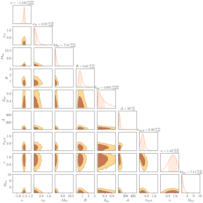
Figure 18: Posterior distribution for our WDM MW satellite population inference from Section 6. Dark (light) contours represent $68\%$ ($95\%$) confidence intervals. We report the galaxy–halo luminosity scatter $\sigma_{M}$ and size scatter $\sigma_{\log R}$ in $\rm{dex}$, the $50\%$ galaxy occupation peak virial mass $\mathcal{M}_{50}$ as $\log(\mathcal{M}_{50}/M_{\rm{\odot}})$, the amplitude of the galaxy–halo size relation $\mathcal{A}$ in parsecs, and the half-mode mass $M_{\mathrm{hm}}$ as $\log(M_{\mathrm{hm}}/M_{\rm{\odot}})$; the faint-end luminosity function slope $\alpha$ (note that this is different than the scale $\alpha$ used in our WDM and FDM SHMF suppression fits), disk disruption efficiency $\mathcal{B}$, galaxy occupation fraction tilt $\mathcal{S}_{\mathrm{gal}}$, and galaxy–halo size relation slope $n$ are dimensionless.

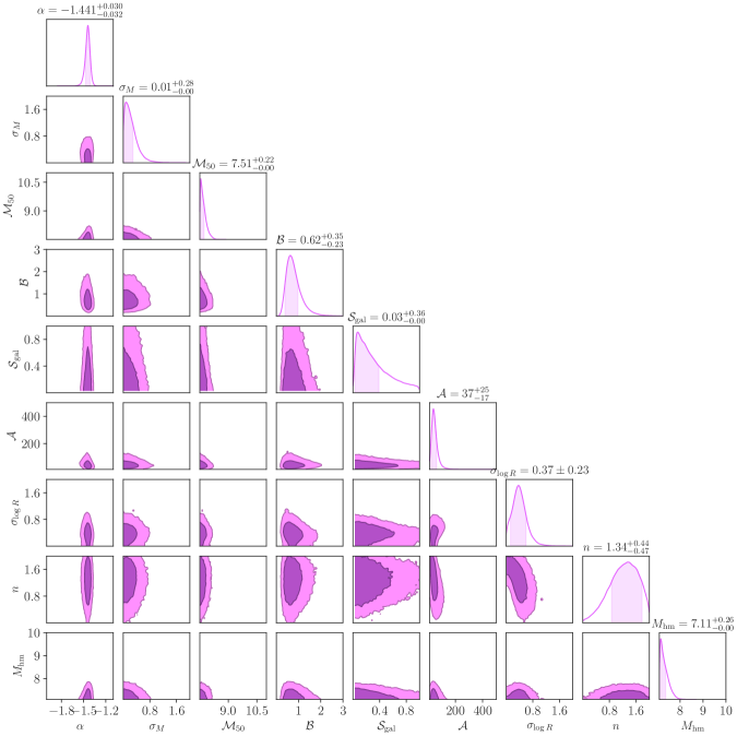
Figure 19: Same as Figure 18 for our FDM MW satellite population inference.

References

- Acevedo et al. (2023) Acevedo, J. F., An, H., Boukhtouchen, Y., et al. 2023, arXiv e-prints, arXiv:2309.08661
- Adhikari et al. (2022) Adhikari, S., Banerjee, A., Boddy, K. K., et al. 2022, arXiv e-prints, arXiv:2207.10638
- Amin & Mirbabayi (2024) Amin, M. A. & Mirbabayi, M. 2024, Phys. Rev. Lett., 132, 221004
- Angulo et al. (2013) Angulo, R. E., Hahn, O., & Abel, T. 2013, MNRAS, 434, 3337
- Armengaud et al. (2017) Armengaud, E., Palanque-Delabrouille, N., Yèche, C., Marsh, D. J. E., & Baur, J. 2017, MNRAS, 471, 4606
- Arvanitaki et al. (2010) Arvanitaki, A., Dimopoulos, S., Dubovsky, S., Kaloper, N., & March-Russell, J. 2010, Phys. Rev. D, 81, 123530
- Arvanitaki et al. (2020) Arvanitaki, A., Dimopoulos, S., Galanis, M., et al. 2020, Phys. Rev. D, 101, 083014
- Banerjee et al. (2022) Banerjee, A., Boddy, K. K., Cyr-Racine, F.-Y., et al. 2022, arXiv e-prints, arXiv:2203.07049
- Banik et al. (2021) Banik, N., Bovy, J., Bertone, G., Erkal, D., & de Boer, T. J. L. 2021, J. Cosmology Astropart. Phys, 2021, 043
- Bechtol et al. (2022) Bechtol, K., Birrer, S., Cyr-Racine, F.-Y., et al. 2022, arXiv e-prints, arXiv:2203.07354
- Behroozi et al. (2013a) Behroozi, P. S., Wechsler, R. H., & Wu, H.-Y. 2013a, ApJ, 762, 109
- Behroozi et al. (2013b) Behroozi, P. S., Wechsler, R. H., Wu, H.-Y., et al. 2013b, ApJ, 763, 18
- Benito et al. (2020) Benito, M., Criado, J. C., Hütsi, G., Raidal, M., & Veermäe, H. 2020, Phys. Rev. D, 101, 103023
- Benson et al. (2013) Benson, A. J., Farahi, A., Cole, S., et al. 2013, MNRAS, 428, 1774
- Boddy & Gluscevic (2018) Boddy, K. K. & Gluscevic, V. 2018, Phys. Rev. D, 98, 083510
- Boddy et al. (2018) Boddy, K. K., Gluscevic, V., Poulin, V., et al. 2018, Phys. Rev. D, 98, 123506
- Bode et al. (2001) Bode, P., Ostriker, J. P., & Turok, N. 2001, ApJ, 556, 93
- Boehm et al. (2001) Boehm, C., Fayet, P., & Schaeffer, R. 2001, Phys. Lett. B, 518, 8
- Bœhm et al. (2002) Bœhm, C., Riazuelo, A., Hansen, S. H., & Schaeffer, R. 2002, Phys. Rev. D, 66, 083505
- Boehm & Schaeffer (2005) Boehm, C. & Schaeffer, R. 2005, A&A, 438, 419
- Boehm et al. (2014) Boehm, C., Schewtschenko, J. A., Wilkinson, R. J., Baugh, C. M., & Pascoli, S. 2014, MNRAS, 445, L31
- Bohr et al. (2021) Bohr, S., Zavala, J., Cyr-Racine, F.-Y., & Vogelsberger, M. 2021, MNRAS, 506, 128
- Bohr et al. (2020) Bohr, S., Zavala, J., Cyr-Racine, F.-Y., et al. 2020, MNRAS, 498, 3403
- Bonaca & Price-Whelan (2024) Bonaca, A. & Price-Whelan, A. M. 2024, arXiv e-prints, arXiv:2405.19410
- Bond & Szalay (1983) Bond, J. R. & Szalay, A. S. 1983, ApJ, 274, 443
- Bose et al. (2016) Bose, S., Hellwing, W. A., Frenk, C. S., et al. 2016, MNRAS, 455, 318
- Boyarsky et al. (2019) Boyarsky, A., Drewes, M., Lasserre, T., Mertens, S., & Ruchayskiy, O. 2019, Progress in Particle and Nuclear Physics, 104, 1
- Brown et al. (2024) Brown, S. T., Fattahi, A., McCarthy, I. G., et al. 2024, MNRAS, 532, 1223
- Brown et al. (2020) Brown, S. T., McCarthy, I. G., Diemer, B., et al. 2020, MNRAS, 495, 4994
- Bryan & Norman (1998) Bryan, G. L. & Norman, M. L. 1998, ApJ, 495, 80
- Buch et al. (2024) Buch, D., Nadler, E. O., Wechsler, R. H., & Mao, Y.-Y. 2024, ApJ, 971, 79
- Bullock (2010) Bullock, J. S. 2010, arXiv e-prints, arXiv:1009.4505
- Bullock & Boylan-Kolchin (2017) Bullock, J. S. & Boylan-Kolchin, M. 2017, ARA&A, 55, 343
- Callingham et al. (2019) Callingham, T. M., Cautun, M., Deason, A. J., et al. 2019, MNRAS, 484, 5453
- Chakrabarti et al. (2022) Chakrabarti, S., Drlica-Wagner, A., Li, T. S., et al. 2022, arXiv e-prints, arXiv:2203.06200
- Colombi et al. (1996) Colombi, S., Dodelson, S., & Widrow, L. M. 1996, ApJ, 458, 1
- Crumrine et al. (2024) Crumrine, W., Nadler, E. O., An, R., & Gluscevic, V. 2024, arXiv e-prints, arXiv:2406.19458
- Cyr-Racine et al. (2016) Cyr-Racine, F.-Y., Sigurdson, K., Zavala, J., et al. 2016, Phys. Rev. D, 93, 123527
- Dalal & Kravtsov (2022) Dalal, N. & Kravtsov, A. 2022, arXiv e-prints, arXiv:2203.05750
- Decant et al. (2022) Decant, Q., Heisig, J., Hooper, D. C., & Lopez-Honorez, L. 2022, J. Cosmology Astropart. Phys, 2022, 041
- Dekker et al. (2022) Dekker, A., Ando, S., Correa, C. A., & Ng, K. C. Y. 2022, Phys. Rev. D, 106, 123026
- Diemand et al. (2005) Diemand, J., Moore, B., & Stadel, J. 2005, Nature, 433, 389
- Dienes et al. (2022) Dienes, K. R., Huang, F., Kost, J., Thomas, B., & Yu, H.-B. 2022, Phys. Rev. D, 106, 123521
- Driskell et al. (2022) Driskell, T., Nadler, E. O., Mirocha, J., et al. 2022, Phys. Rev. D, 106, 103525
- Drlica-Wagner et al. (2019) Drlica-Wagner, A., Mao, Y.-Y., Adhikari, S., et al. 2019, arXiv e-prints, arXiv:1902.01055
- Drlica-Wagner et al. (2020) Drlica-Wagner, A., Bechtol, K., Mau, S., et al. 2020, ApJ, 893, 47
- Du et al. (2018) Du, X., Schwabe, B., Niemeyer, J. C., & Bürger, D. 2018, Phys. Rev. D, 97, 063507
- Du et al. (2024) Du, X., Benson, A., Zeng, Z. C., et al. 2024, Phys. Rev. D, 110, 023019
- Dutton et al. (2020) Dutton, A. A., Buck, T., Macciò, A. V., et al. 2020, MNRAS, 499, 2648
- Dvorkin et al. (2014) Dvorkin, C., Blum, K., & Kamionkowski, M. 2014, Phys. Rev. D, 89, 023519
- Dvorkin et al. (2014) Dvorkin, C., Blum, K., & Kamionkowski, M. 2014, Phys. Rev. D, 89, 023519
- Elgamal et al. (2023) Elgamal, S., Nori, M., Macciò, A. V., Baldi, M., & Waterval, S. 2023, arXiv e-prints, arXiv:2311.03591
- Enzi et al. (2021) Enzi, W., Murgia, R., Newton, O., et al. 2021, MNRAS, 506, 5848
- Erickcek & Sigurdson (2011) Erickcek, A. L. & Sigurdson, K. 2011, Phys. Rev. D, 84, 083503
- Farrar (2022) Farrar, G. R. 2022, arXiv e-prints, arXiv:2201.01334
- Foreman-Mackey et al. (2013) Foreman-Mackey, D., Hogg, D. W., Lang, D., & Goodman, J. 2013, PASP, 125, 306
- Forouhar Moreno et al. (2022) Forouhar Moreno, V. J., Benítez-Llambay, A., Cole, S., & Frenk, C. 2022, MNRAS, 517, 5627
- Frenk et al. (1999) Frenk, C. S., White, S. D. M., Bode, P., et al. 1999, ApJ, 525, 554
- Garrison-Kimmel et al. (2017) Garrison-Kimmel, S., Wetzel, A., Bullock, J. S., et al. 2017, MNRAS, 471, 1709
- Genel et al. (2019) Genel, S., Bryan, G. L., Springel, V., et al. 2019, ApJ, 871, 21
- Gezari et al. (2022) Gezari, S., Bentz, M., De, K., et al. 2022, arXiv e-prints, arXiv:2202.12311
- Gilman et al. (2020) Gilman, D., Birrer, S., Nierenberg, A., et al. 2020, MNRAS, 491, 6077
- Gluscevic & Boddy (2018) Gluscevic, V. & Boddy, K. K. 2018, Phys. Rev. Lett., 121, 081301
- Gluscevic et al. (2019) Gluscevic, V., Ali-Haimoud, Y., Bechtol, K., et al. 2019, BAAS, 51, 134
- Götz & Sommer-Larsen (2003) Götz, M. & Sommer-Larsen, J. 2003, Ap&SS, 284, 341
- Graham et al. (2016) Graham, P. W., Mardon, J., & Rajendran, S. 2016, Phys. Rev. D, 93, 103520
- Green et al. (2004) Green, A. M., Hofmann, S., & Schwarz, D. J. 2004, MNRAS, 353, L23
- Grin et al. (2022) Grin, D., Marsh, D. J. E., & Hlozek, R. 2022, axionCAMB: Modification of the CAMB Boltzmann code, Astrophysics Source Code Library, record ascl:2203.026
- Hahn & Abel (2011) Hahn, O. & Abel, T. 2011, MNRAS, 415, 2101
- He et al. (2023) He, A., Ivanov, M. M., An, R., & Gluscevic, V. 2023, ApJ, 954, L8
- Heston et al. (2024) Heston, S., Horiuchi, S., & Shirai, S. 2024, Phys. Rev. D, 110, 023004
- Hinshaw et al. (2013) Hinshaw, G., Larson, D., Komatsu, E., et al. 2013, ApJS, 208, 19
- Hinton (2016) Hinton, S. R. 2016, The Journal of Open Source Software, 1, 00045
- Hlozek et al. (2015) Hlozek, R., Grin, D., Marsh, D. J. E., & Ferreira, P. G. 2015, Phys. Rev. D, 91, 103512
- Hsueh et al. (2020) Hsueh, J. W., Enzi, W., Vegetti, S., et al. 2020, MNRAS, 492, 3047
- Hu et al. (2000) Hu, W., Barkana, R., & Gruzinov, A. 2000, Phys. Rev. Lett., 85, 1158
- Hui et al. (2017) Hui, L., Ostriker, J. P., Tremaine, S., & Witten, E. 2017, Phys. Rev. D, 95, 043541
- Hunter (2007) Hunter, J. D. 2007, Computing in Science Engineering, 9, 90
- Iršič et al. (2017a) Iršič, V., Viel, M., Haehnelt, M. G., Bolton, J. S., & Becker, G. D. 2017a, Phys. Rev. Lett., 119, 031302
- Iršič et al. (2017b) Iršič, V., Viel, M., Haehnelt, M. G., et al. 2017b, Phys. Rev. D, 96, 023522
- Iršič et al. (2024) Iršič, V., Viel, M., Haehnelt, M. G., et al. 2024, Phys. Rev. D, 109, 043511
- Ivezić et al. (2008) Ivezić, Ž., Kahn, S. M., Tyson, J. A., et al. 2008, ApJ, 873, 111
- Jones et al. (2001) Jones, E., Oliphant, T., Peterson, P., et al. 2001, SciPy: Open source scientific tools for Python, [Online; scipy.org]
- Keeley et al. (2024) Keeley, R. E., Nierenberg, A. M., Gilman, D., et al. 2024, arXiv e-prints, arXiv:2405.01620
- Kelley et al. (2019) Kelley, T., Bullock, J. S., Garrison-Kimmel, S., et al. 2019, MNRAS, 487, 4409
- Kim et al. (2018) Kim, S. Y., Peter, A. H. G., & Hargis, J. R. 2018, Phys. Rev. Lett., 121, 211302
- Klypin et al. (1999) Klypin, A., Kravtsov, A. V., Valenzuela, O., & Prada, F. 1999, ApJ, 522, 82
- Kravtsov (2010) Kravtsov, A. 2010, AdAst, 2010, 281913
- Kulkarni & Ostriker (2022) Kulkarni, M. & Ostriker, J. P. 2022, MNRAS, 510, 1425
- Leo et al. (2017) Leo, M., Baugh, C. M., Li, B., & Pascoli, S. 2017, J. Cosmology Astropart. Phys, 2017, 017
- Lesgourgues (2011) Lesgourgues, J. 2011, arXiv e-prints, arXiv:1104.2932
- Lovell (2020a) Lovell, M. R. 2020a, MNRAS, 493, L11
- Lovell (2020b) Lovell, M. R. 2020b, ApJ, 897, 147
- Lovell et al. (2021) Lovell, M. R., Cautun, M., Frenk, C. S., Hellwing, W. A., & Newton, O. 2021, MNRAS, 507, 4826
- Lovell et al. (2014) Lovell, M. R., Frenk, C. S., Eke, V. R., et al. 2014, MNRAS, 439, 300
- Lovell et al. (2017) Lovell, M. R., Bose, S., Boyarsky, A., et al. 2017, MNRAS, 468, 4285
- Lovell et al. (2019) Lovell, M. R., Barnes, D., Bahé, Y., et al. 2019, MNRAS, 485, 4071
- Lu et al. (2006) Lu, Y., Mo, H. J., Katz, N., & Weinberg, M. D. 2006, MNRAS, 368, 1931
- Maamari et al. (2021) Maamari, K., Gluscevic, V., Boddy, K. K., Nadler, E. O., & Wechsler, R. H. 2021, ApJ, 907, L46
- Mansfield et al. (2024) Mansfield, P., Darragh-Ford, E., Wang, Y., et al. 2024, ApJ, 970, 178
- Mao et al. (2015) Mao, Y.-Y., Williamson, M., & Wechsler, R. H. 2015, ApJ, 810, 21
- Marsh (2011) Marsh, D. J. E. 2011, Phys. Rev. D, 83, 123526
- Marsh (2016) Marsh, D. J. E. 2016, Phys. Rep., 643, 1
- May & Springel (2021) May, S. & Springel, V. 2021, MNRAS, 506, 2603
- May & Springel (2023) May, S. & Springel, V. 2023, MNRAS, 524, 4256
- McDermott et al. (2011) McDermott, S. D., Yu, H.-B., & Zurek, K. M. 2011, Phys. Rev. D, 83, 063509
- McKinney (2010) McKinney, W. 2010, in Proceedings of the 9th Python in Science Conference, ed. S. van der Walt & J. Millman, 51
- Meshveliani et al. (2023) Meshveliani, T., Lovell, M. R., Crain, R. A., & Pfeffer, J. 2023, arXiv e-prints, arXiv:2312.00150
- Moore et al. (1999) Moore, B., Ghigna, S., Governato, F., et al. 1999, ApJ, 524, L19
- Moore & Slatyer (2024) Moore, M. & Slatyer, T. R. 2024, Phys. Rev. D, 110, 023515
- Murgia et al. (2017) Murgia, R., Merle, A., Viel, M., Totzauer, M., & Schneider, A. 2017, J. Cosmology Astropart. Phys, 2017, 046
- Nadler et al. (2021a) Nadler, E. O., Birrer, S., Gilman, D., et al. 2021a, ApJ, 917, 7
- Nadler et al. (2019a) Nadler, E. O., Gluscevic, V., Boddy, K. K., & Wechsler, R. H. 2019a, ApJ, 878, L32
- Nadler et al. (2024) Nadler, E. O., Gluscevic, V., Driskell, T., et al. 2024, ApJ, 967, 61
- Nadler et al. (2019b) Nadler, E. O., Mao, Y.-Y., Green, G. M., & Wechsler, R. H. 2019b, ApJ, 873, 34
- Nadler et al. (2018) Nadler, E. O., Mao, Y.-Y., Wechsler, R. H., Garrison-Kimmel, S., & Wetzel, A. 2018, ApJ, 859, 129
- Nadler et al. (2020) Nadler, E. O., Wechsler, R. H., Bechtol, K., et al. 2020, ApJ, 893, 48
- Nadler et al. (2021b) Nadler, E. O., Drlica-Wagner, A., Bechtol, K., et al. 2021b, Phys. Rev. Lett., 126, 091101
- Nadler et al. (2023) Nadler, E. O., Mansfield, P., Wang, Y., et al. 2023, ApJ, 945, 159
- Nagai & Kravtsov (2005) Nagai, D. & Kravtsov, A. V. 2005, ApJ, 618, 557
- Navarro et al. (1997) Navarro, J. F., Frenk, C. S., & White, S. D. M. 1997, ApJ, 490, 493
- Newton et al. (2024) Newton, O., Lovell, M. R., Frenk, C. S., et al. 2024, arXiv e-prints, arXiv:2408.16042
- Newton et al. (2021) Newton, O., Leo, M., Cautun, M., et al. 2021, J. Cosmology Astropart. Phys, 2021, 062
- Nguyen et al. (2021) Nguyen, D. V., Sarnaaik, D., Boddy, K. K., Nadler, E. O., & Gluscevic, V. 2021, Phys. Rev. D, 104, 103521
- Nori & Baldi (2018) Nori, M. & Baldi, M. 2018, MNRAS, 478, 3935
- Nori et al. (2023) Nori, M., Macciò, A. V., & Baldi, M. 2023, MNRAS, 522, 1451
- Onions et al. (2012) Onions, J., Knebe, A., Pearce, F. R., et al. 2012, MNRAS, 423, 1200
- Passaglia & Hu (2022) Passaglia, S. & Hu, W. 2022, Phys. Rev. D, 105, 123529
- Pedregosa et al. (2011) Pedregosa, F., Varoquaux, G., Gramfort, A., et al. 2011, Journal of Machine Learning Research
- Pontzen & Governato (2012) Pontzen, A. & Governato, F. 2012, MNRAS, 421, 3464
- Pontzen et al. (2013) Pontzen, A., Roškar, R., Stinson, G., & Woods, R. 2013, pynbody: N-Body/SPH analysis for python, Astrophysics Source Code Library, record ascl:1305.002
- Powell et al. (2023) Powell, D. M., Vegetti, S., McKean, J. P., et al. 2023, MNRAS, 524, L84
- Rogers et al. (2022) Rogers, K. K., Dvorkin, C., & Peiris, H. V. 2022, Phys. Rev. Lett., 128, 171301
- Rogers et al. (2023) Rogers, K. K., Hložek, R., Laguë, A., et al. 2023, J. Cosmology Astropart. Phys, 2023, 023
- Rogers & Peiris (2021) Rogers, K. K. & Peiris, H. V. 2021, Phys. Rev. Lett., 126, 071302
- Rogers & Poulin (2023) Rogers, K. K. & Poulin, V. 2023, arXiv e-prints, arXiv:2311.16377
- Rose et al. (2024) Rose, J. C., Torrey, P., Villaescusa-Navarro, F., et al. 2024, arXiv e-prints, arXiv:2405.00766
- Rubira et al. (2023) Rubira, H., Mazoun, A., & Garny, M. 2023, J. Cosmology Astropart. Phys, 2023, 034
- Schewtschenko et al. (2016) Schewtschenko, J. A., Baugh, C. M., Wilkinson, R. J., et al. 2016, MNRAS, 461, 2282
- Schewtschenko et al. (2015) Schewtschenko, J. A., Wilkinson, R. J., Baugh, C. M., Bœhm, C., & Pascoli, S. 2015, MNRAS, 449, 3587
- Schive et al. (2014) Schive, H.-Y., Chiueh, T., & Broadhurst, T. 2014, Nature Physics, 10, 496
- Schive et al. (2016) Schive, H.-Y., Chiueh, T., Broadhurst, T., & Huang, K.-W. 2016, ApJ, 818, 89
- Schneider (2016) Schneider, A. 2016, J. Cosmology Astropart. Phys, 2016, 059
- Schneider et al. (2012) Schneider, A., Smith, R. E., Macciò, A. V., & Moore, B. 2012, MNRAS, 424, 684
- Schutz (2020) Schutz, K. 2020, Phys. Rev. D, 101, 123026
- Schwabe et al. (2020) Schwabe, B., Gosenca, M., Behrens, C., Niemeyer, J. C., & Easther, R. 2020, Phys. Rev. D, 102, 083518
- Schwabe & Niemeyer (2022) Schwabe, B. & Niemeyer, J. C. 2022, Phys. Rev. Lett., 128, 181301
- Spergel et al. (2015) Spergel, D., Gehrels, N., Baltay, C., et al. 2015, arXiv e-prints, arXiv:1503.03757
- Springel (2005) Springel, V. 2005, MNRAS, 364, 1105
- Springel et al. (2008) Springel, V., Wang, J., Vogelsberger, M., et al. 2008, MNRAS, 391, 1685
- Srisawat et al. (2013) Srisawat, C., Knebe, A., Pearce, F. R., et al. 2013, MNRAS, 436, 150
- Stücker et al. (2022) Stücker, J., Angulo, R. E., Hahn, O., & White, S. D. M. 2022, MNRAS, 509, 1703
- Tulin & Yu (2018) Tulin, S. & Yu, H.-B. 2018, Phys. Rep., 730, 1
- van den Bosch & Jiang (2016) van den Bosch, F. C. & Jiang, F. 2016, MNRAS, 458, 2870
- van der Walt et al. (2011) van der Walt, S., Colbert, S. C., & Varoquaux, G. 2011, Computing in Science Engineering, 13, 22
- Vegetti et al. (2023) Vegetti, S., Birrer, S., Despali, G., et al. 2023, arXiv e-prints, arXiv:2306.11781
- Viel et al. (2013) Viel, M., Becker, G. D., Bolton, J. S., & Haehnelt, M. G. 2013, Phys. Rev. D, 88, 043502
- Viel et al. (2005) Viel, M., Lesgourgues, J., Haehnelt, M. G., Matarrese, S., & Riotto, A. 2005, Phys. Rev. D, 71, 063534
- Villasenor et al. (2023) Villasenor, B., Robertson, B., Madau, P., & Schneider, E. 2023, Phys. Rev. D, 108, 023502
- Vogel & Abazajian (2023) Vogel, C. M. & Abazajian, K. N. 2023, Phys. Rev. D, 108, 043520
- Vogelsberger et al. (2016) Vogelsberger, M., Zavala, J., Cyr-Racine, F.-Y., et al. 2016, MNRAS, 460, 1399
- Wang & White (2007) Wang, J. & White, S. D. M. 2007, MNRAS, 380, 93
- Wang et al. (2024) Wang, Y., Mansfield, P., Nadler, E. O., et al. 2024, arXiv e-prints, arXiv:2408.01487
- Webb & Bovy (2020) Webb, J. J. & Bovy, J. 2020, MNRAS, 499, 116
- Wechsler et al. (2002) Wechsler, R. H., Bullock, J. S., Primack, J. R., Kravtsov, A. V., & Dekel, A. 2002, ApJ, 568, 52
- Zhang et al. (2024) Zhang, C., Zu, L., Chen, H.-Z., Tsai, Y.-L. S., & Fan, Y.-Z. 2024, J. Cosmology Astropart. Phys, 2024, 003
- Zimmermann et al. (2024) Zimmermann, T., Alvey, J., Marsh, D. J. E., Fairbairn, M., & Read, J. I. 2024, arXiv e-prints, arXiv:2405.20374