Blast.jl: Beyond Limber Angular power Spectra Toolkit. A fast and efficient algorithm for $3\times 2$ pt analysis.

Abstract

The advent of next-generation photometric and spectroscopic surveys is approaching, bringing more data with tighter error bars. As a result, theoretical models will become more complex, incorporating additional parameters, which will increase the dimensionality of the parameter space and make posteriors more challenging to explore. Consequently, the need to improve and speed up our current analysis pipelines will grow. In this work, we focus on the $3\times 2$ pt statistics, a summary statistic that has become increasingly popular in recent years due to its great constraining power. These statistics involve calculating angular two-point correlation functions for the auto- and cross-correlations between galaxy clustering and weak lensing. The corresponding model is determined by integrating the product of the power spectrum and two highly-oscillating Bessel functions over three dimensions, which makes the evaluation particularly challenging. Typically, this difficulty is circumvented by employing the so-called Limber approximation, which is an important source of error. We present Blast.jl, an innovative and efficient algorithm for calculating angular power spectra without employing the Limber approximation or assuming a scale-dependent growth rate, based on the use of Chebyshev polynomials. The algorithm is compared with the publicly available beyond-Limber codes, whose performances were recently tested by the LSST Dark Energy Science Collaboration in the N5K challenge. At similar accuracy, Blast.jl is $\approx 10$-$15\times$ faster than the winning method of the challenge, also showing excellent scaling with respect to various hyper-parameters.

1 Introduction

Next-generation spectroscopic and photometric surveys, such as Euclid (Mellier et al., 2024), LSST (Ivezic et al., 2019), the Nancy Grace Roman Space Telescope (Wang et al., 2022) and DESI (Levi et al., 2019), aim to achieve high-accuracy measurements of Large Scale Structure (LSS). These surveys measure various tracers, including galaxy density and weak lensing, across wider areas of the sky and at increasingly deep redshifts. Traditional cosmological parameter estimation relies on the power spectrum to compress the data into a reduced form, containing the majority of the desired information. For surveys that rely on photometric redshifts, there is little radial information, and the angular power spectra ($C_{\ell}$) within and between different tomographic redshift bins are sufficient to retain relevant information. This is the main idea behind $3\times 2$ pt statistics, which apply this technique for different combinations of tracers: galaxy clustering, lensing shear-shear correlation, and galaxy-galaxy lensing cross-correlation. A major drawback that comes with using $3\times 2$ pt statistics is the numerical computation of the model, which requires the calculation of a highly oscillating three-dimensional integral. A common work-around is the Limber approximation (Limber, 1953) which assumes that modes between structures at different epochs do not contribute to the line-of-sight integration. This approximation reduces the highly-oscillatory 3D integrand into a smooth 1D integrand, enabling faster computation. However, it introduces significant errors, particularly on large angular scales (low $\ell$’s). Therefore, a more accurate evaluation of the $3\times 2$ pt model is essential to better control systematics and to preserve the information gain from new surveys. We need not only a precise computation of the $3\times 2$ pt data vector but also a method that is as fast as possible. In fact, if this model is to be used to perform parameter inference through Monte Carlo Markov Chains (MCMC), we expect to perform millions of evaluations, so the task of speeding up the computation of the full non-Limber integral is very important as it will make cosmological analyses with $3\times 2$ pt computationally feasible. As an example, in the recent Euclid overview paper (Mellier et al., 2024), $3\times 2$ pt statistics were computed using the Limber approximation and the MCMC took $0.5$ million CPU hours to converge.

In light of this problem, the LSST Dark Energy Science Collaboration (Ivezic et al., 2019) in 2020 launched the N5K challenge (Leonard et al., 2023), with the aim of assessing what the state of the art of non-Limber integration is, and determine which is the best method to incorporate in their pipeline. In this work we present a novel algorithm, implemented in the Blast.jl code, for non-Limber integration, as a late entry to the challenge. Blast.jl builds on the idea of performing a decomposition of the power spectrum on the convenient basis of the Chebyshev polynomials. Thanks to this decomposition, the hardest part of the integral becomes cosmology-independent and can therefore be pre-computed only once.
The paper is structured as follows: in Sec. 2 the model for $3\times 2$ pt statistics is worked out in detail. The Limber approximation and its regimes of validity are also discussed. In Section 3 our new method, which is based on the decomposition of the power spectrum on the basis of Chebyshev polynomials, is introduced. Sec. 4 outlines the details of the N5K challenge, discussing the set-up, the specific configurations, the evaluation metric, and the three algorithms that took part in the challenge. We then present how Blast.jl performs and scales with respect to different parameters by rigorously comparing it to the other entries in Sec. 5 and 6. Conclusions are drawn in Sec. 7.

2 Theory

2.1 Angular Power Spectra

To derive the model for $3\times 2$ pt analysis, we begin by noting that any observable $A(\mathbf{x})$ defined on the sky can be expanded using spherical harmonics for scalar fields or spin-weighted spherical harmonics in the more general case. For scalar fields on the sphere, we restrict ourselves to the standard spherical harmonics, which form a complete and orthonormal basis for the total angular momentum operator, first introduced by Hu & White (1997). The expansion coefficients are:

$$A_{\ell,m}=N(\ell)Y_{\ell,m}(\hat{n})e^{\mathrm{i}\mathbf{k\cdot x}},$$ (1)

where $N(\ell)$ is a $\ell$-dependent numerical prefactor and $Y_{\ell,m}(\hat{n})$ are the spherical harmonics. Then, if we have two scalar fields defined on the sphere $A(\mathbf{x})$ and $B(\mathbf{x})$, it is possible to expand both of them in spherical harmonics and compute the angular cross-correlation power spectrum:

$$\begin{split}C_{\mathrm{AB}}(\ell)&=\langle A_{\ell,m}B_{\ell,m}^{*}\rangle=\\ &=N(\ell)\int_{0}^{\infty}\mathrm{d}k\,k^{2}P_{\mathrm{AB}}(k,\chi_{1},\chi_{2})\frac{j_{\ell}(k\chi_{1})j_{\ell}(k\chi_{2})}{(k\chi_{1})^{\alpha}(k\chi_{2})^{\beta}}.\end{split}$$ (2)

Here, $P_{\mathrm{AB}}(k,\chi_{1},\chi_{2})$ is the $3$D power spectrum, containing the $2$ pt cosmological information, $\alpha$ and $\beta$ can assume different values depending on the probe that is considered, in particular $0$ for clustering and $2$ for lensing, and $j_{\ell}(x)$ are the spherical Bessel functions, which are present in this expression due to the use of the plane wave expansion:

$$e^{\mathrm{i}\mathbf{k\cdot r}}=4\pi\sum_{\ell=0}^{\infty}\sum_{m=-\ell}^{\ell}\mathrm{i}^{\ell}j_{\ell}(kr)Y_{\ell}^{m}(\hat{k})Y_{\ell}^{m*}(\hat{r}).$$ (3)

Finally, we need to account for the fact that a real survey measures number counts and cosmic shear in different tomographic redshift bins. Those measurements are described by averaging over some survey-specific window functions $W_{i}^{A}(\chi)$ that only depend on geometry. The final expression for the angular power spectrum is then a triple integral of the form:

$$\begin{split}C_{ij}^{\mathrm{AB}}(\ell)&=N(\ell)\int_{0}^{\infty}\mathrm{d}\chi_{1}W_{i}^{\mathrm{A}}(\chi_{1})\int_{0}^{\infty}\mathrm{d}\chi_{2}W_{j}^{\mathrm{B}}(\chi_{2})\times\\ &\quad\times\int_{0}^{\infty}\mathrm{d}k\,k^{2}P_{\mathrm{AB}}(k,\chi_{1},\chi_{2})\frac{j_{\ell}(k\chi_{1})j_{\ell}(k\chi_{2})}{(k\chi_{1})^{\alpha}(k\chi_{2})^{\beta}}.\end{split}$$ (4)

Due to the nature of the spherical Bessel functions, which are highly oscillating and slowly damped, the evaluation of the integral is computationally challenging.

2.2 The Limber Approximation

The Limber approximation (Limber, 1953) is commonly employed to simplify the integral in Eq. (4) and reduce it to a $1$D integral by approximating the spherical Bessel functions around their first peak, located at $k\chi\approx\ell+1/2$. The peak gives the largest contribution to the integral. In fact, due to the highly-oscillatory nature of the functions, there are large cancellations that cause the other contributions to be very small (LoVerde & Afshordi, 2008). We can then write:

$$j_{\ell}(x)\approx\sqrt{\frac{\pi}{2\ell+1}}\delta_{\mathrm{D}}\left(\ell+\frac{1}{2}-x\right),$$ (5)

$\delta_{\mathrm{D}}(x)$ being the Dirac delta function. Another equivalent way to get this result is to consider orthogonality relations of the spherical Bessel functions:

$$\int_{0}^{\infty}\mathrm{d}k\,k^{2}j_{\ell}(k\chi_{1})j_{\ell}(k\chi_{2})=\frac{2\delta_{\mathrm{D}}(\chi_{1}-\chi_{2})}{\pi\chi_{1}\chi_{2}}.$$ (6)

Applying this approximation, Eq. (4) reduces to:

$$C^{\mathrm{AB}}_{ij}(\ell)\approx\int_{0}^{\infty}\frac{\mathrm{d}\chi}{\chi^{2}}K_{i}^{\mathrm{A}}(\chi)K_{j}^{\mathrm{B}}(\chi)P_{\mathrm{AB}}\left(k_{\ell},z\right).$$ (7)

We defined $k_{\ell}\equiv(\ell+1/2)/f(\chi)$, $f(\chi)$ is a general function that depends on the cosmological model. In the case of the standard $\Lambda$CDM model, which we will assume here, $f(\chi)=\chi$. This integral is one dimensional and does not contain oscillatory function, making it inherently easier and faster to compute. The regimes of validity of this approximation are well understood (LoVerde & Afshordi, 2008). The Limber approximation, which sets $\chi_{1}=\chi_{2}$, works well especially for higher $\ell$’s, where the feature that the integrands have for $\chi_{1}=\chi_{2}$ gets increasingly sharp. In addition, for high multipoles $\ell$ the flat sky approximation is valid. Moreover, the approximation works best when the kernels $K_{i}^{\mathrm{A}}$ are broad in comoving distance (i.e., the approximation works best for the weak lensing sample rather than the clustering one) and for the auto-correlation within a redshift bin, as the kernels $K_{i}^{\mathrm{A}}$, $K_{j}^{\mathrm{A}}$ are superimposed in comoving distance.

LoVerde & Afshordi (2008) developed a more refined approximation of the integral, the extended Limber approximation. The idea is to Taylor expand the spherical Bessel function around its primary peak and keep higher orders of the expansion. Performing this calculation and defining $\nu\equiv kr=\ell+1/2$, one finds:

$$\begin{split}C^{\mathrm{AB}}_{ij}(\ell)&=N(\ell)\int\frac{\mathrm{d}\chi}{\chi^{2}}K_{i}(\chi)K_{j}(\chi)P_{\mathrm{AB}}\left(k=\frac{\nu}{\chi}\right)\Biggl{\{}1+\\ &\quad+\frac{1}{\nu^{2}}\left[\frac{\chi^{2}}{2}\left(\frac{\tilde{K}_{i}^{{}^{\prime\prime}}(\chi)}{\tilde{K}_{i}(\chi)}+\frac{\tilde{K}_{j}^{{}^{\prime\prime}}(\chi)}{\tilde{K}_{j}(\chi)}\right)\right.+\\ &\quad\left.+\frac{\chi^{3}}{6}\left(\frac{\tilde{K}_{i}^{{}^{\prime\prime\prime}}(\chi)}{\tilde{K}_{i}(\chi)}+\frac{\tilde{K}_{j}^{{}^{\prime\prime\prime}}(\chi)}{\tilde{K}_{j}(\chi)}\right)\right]\Biggr{\}}.\end{split}$$ (8)

Where we defined

$$\tilde{K}(\chi)\equiv\frac{K(\chi)}{\sqrt{\chi}}.$$ (9)

This expression shows the first-order correction to the standard Limber approximation, which brings the error from $\mathcal{O}(\ell^{-2})$ to $\mathcal{O}(\ell^{-4})$. While the higher-order Limber can help reduce the error and improve the speed of convergence for higher $\ell$, it does not necessarily make it accurate in the low-$\ell$ regime (LoVerde & Afshordi, 2008).

3 The Blast.jl algorithm

We propose a new algorithm to compute the full non-Limber angular power spectra for galaxy clustering, galaxy-galaxy lensing and cosmic shear, and then discuss the implementation of this idea.

3.1 The Algorithm

Let us start by explicitly expressing the three integrals, incorporating the appropriate $\ell$-dependent prefactors and the correct $k$-dependency. For galaxy clustering, we get:

$$\begin{split}C_{ij}^{gg}(\ell)&=\frac{2}{\pi}\int_{0}^{\infty}\mathrm{d}\chi_{1}W_{i}^{g}(\chi_{1})\int_{0}^{\infty}\mathrm{d}\chi_{2}W_{j}^{g}(\chi_{2})\times\\ &\quad\times\int_{0}^{\infty}\mathrm{d}k\,k^{2}P_{\mathrm{AB}}(k,\chi_{1},\chi_{2})j_{\ell}(k\chi_{1})j_{\ell}(k\chi_{2}).\end{split}$$ (10)

The kernel has the form:

$$W_{i}^{g}(\chi)=H(z)n_{i}(z)b_{g}(z),$$ (11)

$H(z)$ is the expansion rate, $n_{i}(z)$ is the redshift distribution of the sample in the $i$-th clustering redshift bin, and $b_{g}(z)$ is the linear galaxy bias.

For weak lensing:

$$\begin{split}C_{ij}^{ss}(\ell)&=\frac{2(\ell+2)!}{\pi(\ell-2)!}\int_{0}^{\infty}\mathrm{d}\chi_{1}W_{i}^{s}(\chi_{1})\int_{0}^{\infty}\mathrm{d}\chi_{2}W_{j}^{s}(\chi_{2})\times\\ &\quad\times\int_{0}^{\infty}\mathrm{d}k\,k^{2}P_{\mathrm{AB}}(k,\chi_{1},\chi_{2})\frac{j_{\ell}(k\chi_{1})}{(k\chi_{1})^{2}}\frac{j_{\ell}(k\chi_{2})}{(k\chi_{2})^{2}}.\end{split}$$ (12)

For the shear sample, the kernel has shape:

$$W_{i}^{s}(\chi)=\frac{3H_{0}^{2}\Omega_{m}}{2a}\chi\int_{z}^{\infty}dz^{\prime}n_{i}(z^{\prime})\frac{\chi(z^{\prime})-\chi}{\chi(z^{\prime})}.$$ (13)

Finally, for the cross-correlation of the two samples, the angular power spectrum is:

$$\begin{split}C_{ij}^{gs}(\ell)&=\frac{2}{\pi}\sqrt{\frac{(\ell+2)!}{(\ell-2)!}}\int_{0}^{\infty}\mathrm{d}\chi_{1}W_{i}^{g}(\chi_{1})\int_{0}^{\infty}\mathrm{d}\chi_{2}W_{j}^{s}(\chi_{2})\times\\ &\quad\times\int_{0}^{\infty}\mathrm{d}k\,k^{2}P_{\mathrm{AB}}(k,\chi_{1},\chi_{2})\frac{j_{\ell}(k\chi_{1})}{(k\chi_{1})^{2}}j_{\ell}(k\chi_{2}).\end{split}$$ (14)

Our strategy to solve the integrals specified in Eq. (10)-(14) will be the following: we will first tackle the inner $k$-integral containing the two Bessel functions. This is the bottleneck of the computation. Having solved that, the two outer integrals over $\chi_{1}$-$\chi_{2}$ will be solved with standard quadrature techniques. The algorithm uses a Chebyshev decomposition of the power spectrum to break the integral into terms that can be pre-computed. Once these terms are available, updating for any new power spectrum only requires recalculating the decomposition coefficients, which takes up very little computing time. Chebyshev polynomials are an advantageous choice of basis as, thanks to their properties, they have close to optimal approximation ability. While the computation of the Chebyshev coefficients requires a specific grid in $k$, this approach does not impose a specific grid for the other two integration variables. This is unlike other decomposition-based algorithms, such as FFTLog, which require a logarithmic spacing of the grid. The polynomials are defined as:

$$T_{n}(\cos\theta)=\cos(n\theta),$$ (15)

or, equivalently, by the recursion relation:

$$T_{0}(x) =1,$$ (16)

$$T_{1}(x) =x,$$

$$T_{n+1}(x) =2xT_{n}(x)-T_{n-1}(x).$$

They form a complete and orthonormal basis, widely used in approximation theory due to the many mathematical properties of the polynomials, which ensure high accuracy in the approximation. For an in-depth treatment of approximation theory using Chebyshev polynomials, see Trefethen (2019). Below, we outline the key definitions. In general, a function that is (Lipschitz) continuous in $[-1,1]$ has a unique representation as a Chebyshev series:

$$f(x)=\sum_{n=0}^{\infty}a_{n}T_{n}(x),$$ (17)

with

$$a_{n}\equiv\frac{2}{\pi}\int_{-1}^{1}\frac{f(x)T_{n}(x)}{\sqrt{1-x^{2}}}\mathrm{d}x.$$ (18)

However, to approximate $f(x)$, one can also use the polynomial obtained by interpolation in the Chebyshev points, a set of points defined as:

$$x_{k}=\cos{\left(\frac{2k+1}{2n}\pi\right)}\,\,\,k=0,...,n-1.$$ (19)

Those points are defined in $[-1,1]$ and have the property of being more dense close to the edges of the interval. The polynomial interpolated in $k$ Chebyshev points is:

$$p_{k}(x)=\sum_{n=0}^{n_{\mathrm{max}}}c_{n}T_{n}(x).$$ (20)

We highlight that $a_{n}$ and $c_{n}$ are different sets of coefficients (see the definitions in Eq. (17)-(20)). However, using the properties of Chebyshev polynomials, one can show (Trefethen, 2019) that $a_{n}$ and $c_{n}$ are related by:

$$c_{n}=a_{n}+(a_{n+2k}+a_{n+4k}+...)+(a_{-n+2k}+a_{-n+4k}+...)$$ (21)

for $1\leq n\leq k-1$. That is, the coefficients in the infinite series expansion are reassigned to their aliases of degree $<k$. This property is the reason why the Chebyshev polynomials are so widely used in approximation theory, as they are more accurate than any other method when fixing the number of interpolation points (Trefethen, 2019). In this specific problem, we approximate the power spectrum by interpolation in the Chebyshev points (Eq. (20)). This choice is driven by the fact that the coefficients $c_{n}(\chi_{1},\chi_{2};\theta)$ are evaluated through a Discrete Fourier Transform (DFT) (Press, 2007; Frigo & Johnson, 1997):

$$c_{n}(\chi_{1},\chi_{2})=\sum_{j=0}^{N-1}P(k_{j},\chi_{1},\chi_{2})e^{2\mathrm{i}\pi jn/N}.$$ (22)

The choice of the sampling points $k_{j}$ for the power spectrum will be motivated in the next section. Computing a FFT is much more efficient than evaluating the integrals defining the coefficients $a_{n}$ (Eq. (18)), which justifies our approach. The power spectrum, a (Lipschitz) continuous function over the interval $[k_{\text{min}},k_{\text{max}}]$ (which can be remapped in $[-1,1]$), in the basis of the Chebyshev polynomials becomes:

$$P(k,\chi_{1},\chi_{2};\theta)\approx\sum_{n=0}^{n_{\text{max}}}c_{n}(\chi_{1},\chi_{2};\theta)T_{n}(k),$$ (23)

where $\theta$ represents a generic set of cosmological parameters. This decomposition enables a clear separation of geometric and cosmological components in the integrals, simplifying the overall calculation. We can write:

$$w^{\mathrm{AB}}_{\ell}(\chi_{1},\chi_{2};\theta)\equiv\sum_{n=0}^{n_{\mathrm{max}}}c_{n}(\chi_{1},\chi_{2};\theta)\tilde{T}^{\mathrm{AB}}_{n;\,\ell}(\chi_{1},\chi_{2})\,,$$ (24)

where we defined:

$$\tilde{T}^{\mathrm{AB}}_{n;\,\ell}(\chi_{1},\chi_{2})\equiv\int_{k_{\mathrm{min}}}^{k_{\mathrm{max}}}\mathrm{d}k\,f^{\mathrm{AB}}(k)T_{n}(k)j_{\ell}(k\chi_{1})j_{\ell}(k\chi_{2})\,,$$ (25)

with:

$$f^{\mathrm{AB}}(k)=\begin{cases}k^{2}&\mathrm{AB}=gg\,,\\ 1/k^{2}&\mathrm{AB}=ss\,,\\ 1&\mathrm{AB}=gs\,.\end{cases}$$ (26)

Here $w_{\mathrm{AB}}(\ell)$, which is commonly called “projected matter density”, represents the inner integral in $k$. As evident from Eq. (24), the dependence on the cosmological parameters is only present in the coefficients of the Chebyshev expansion of the power spectrum $c_{n}(\chi_{1},\chi_{2};\theta)$, while $\tilde{T}^{\mathrm{AB}}_{n;\,\ell}(\chi_{1},\chi_{2})$ is cosmology-independent as it is the integral of the two Bessel functions against the Chebyshev polynomials. This is the key idea of the algorithm: the $\tilde{T}^{\mathrm{AB}}_{n;\,\ell}(\chi_{1},\chi_{2})$ integrals are still challenging to compute for the presence of the Bessel functions, but they can be computed once-for-all.

The last ingredient for a successful computation of the integral is a change of variable: introducing $R\equiv\chi_{2}/\chi_{1}$, we can switch from the $\chi_{1}$-$\chi_{2}$ to the $\chi$-$R$ basis, which allows for a better sampling of the regions that most contribute to the integral, i.e., when $\chi_{1}\approx\chi_{2}$ (or, equivalently, $R\approx 1$). For more details on this coordinate change, see Appendix A.
In these new variables, the integral becomes:

$$\begin{split}C_{ij}^{\mathrm{AB}}(\ell)&=\int_{0}^{\infty}d\chi\int_{0}^{1}dR\,\chi\left[\mathcal{K}_{i}^{\mathrm{A}}(\chi)\mathcal{K}_{j}^{\mathrm{B}}(R\chi)+\right.\\ &\quad\quad\left.+\mathcal{K}_{j}^{\mathrm{B}}(\chi)\mathcal{K}_{i}^{\mathrm{A}}(R\chi)\right]w_{\ell}^{\mathrm{AB}}(\chi,R\chi)\,,\end{split}$$ (27)

with:

$$\mathcal{K}_{i}^{\mathrm{A}}(\chi)=\begin{cases}K_{i}^{\mathrm{A}}(\chi)&\text{for clustering}\,,\\ K_{i}^{\mathrm{A}}(\chi)/\chi^{2}&\text{for lensing}\,.\end{cases}$$ (28)

3.2 The implementation

The challenge that we need to face is now the computation of $\tilde{T}^{\mathrm{AB}}_{n;\,\ell}(k)$, the integrals of the two Bessel functions and the Chebyshev polynomials, with the appropriate $k$-factor for each case. Those integrals need to be computed with high accuracy as they constitute the central step of the algorithm. We performed this integration using the Clenshaw-Curtis quadrature rule (Clenshaw & Curtis, 1960) and $N=2^{15}+1$ points in the interval $k_{\text{min}}-k_{\text{max}}$. The value for $k_{\text{min}}$ is $3.571\times 10^{-4}$, and $k_{\text{max}}$ is $15.385$; the choice of those values will be motivated in Section 4. $N=2^{15}+1$ is the value that provides best balance between accuracy and performance for our purposes. In this setting, all the $\tilde{T}^{\mathrm{AB}}_{n;\,\ell}(k)$ can be computed on a laptop in $\approx 1$-$2$ hours with $n_{\text{max}}$, the number of Chebyshev polynomials in the power spectrum approximation, fixed to $120$. How the accuracy scales with respect to the parameter $N$ is discussed in Appendix C.
As it is the central part of the algorithm, we highlight that, whichever the choice of $N$ and $n_{\text{max}}$, this computation is only to be performed once. It is also worth mentioning that the projected matter densities $w_{\ell}^{\mathrm{AB}}(\chi,R\chi)$ that we computed were validated using two independent and well-established codes: TWOFAST (Grasshorn Gebhardt & Jeong, 2018) and QuadOsc (Press, 2007). TWOFAST is a Julia implementation of the FFTLog algorithm (Talman, 1978; Hamilton, 2000), that will be discussed below. QuadOsc solves the problem of the highly oscillatory integrand by integrating between its zero-crossings and successively adding up the contributions. Our evaluation of the integral was found to be in excellent agreement with both codes, confirming the validity of our new approach.

To obtain the angular power spectrum coefficients, the final step is to perform the two outer integrals in $\chi$ and $R=\chi_{2}/\chi_{1}$. The integrals do not present oscillatory functions so they can be performed with standard quadrature rules. For the integral in $\chi$, the Simpson rule (Press, 2007) is sufficient as the integrand is a smooth function in $\chi$. To perform this integral, we placed $96$ evenly spaced points for $\chi\in(26,7000)\,\,\mathrm{Mpc/h}$.
This is not true for the $R$ coordinate, in fact, the integral presents a sharp feature for $R\approx 1$ ($\chi_{1}\approx\chi_{2}$). It arises because the biggest contribution to the integral comes from regions at the same cosmic time, as one can see from Fig. 6. We define the points in $R$ in the interval $(-1,1)$ as the Chebyshev points, defined in Eq. (19). As anticipated, they have the property of being more densely distributed close to the edges of the interval, making them well-suited for this specific task. By definition, $R$ is positive, so to account for that we placed $97$ Chebyshev points in $[-1,1]$ and only kept the strictly positive ones: $48$ points in $(0,1]$. There is another advantage to this choice: since the projected matter density $w_{\ell}^{\mathrm{AB}}(\chi,R)$ is evaluated on Chebyshev points in $R$, we can perform the $R$-integral using the Clenshaw-Curtis quadrature rule (Clenshaw & Curtis, 1960), a method that is based on Chebyshev polynomials and has better convergence properties than the second-order Simpson rule.The change of coordinate is key for a successful evaluation of the angular power spectra, as is shown in Appendix A. In fact, when working with the $\chi_{1}$-$\chi_{2}$ coordinates, $500$ points in both $\chi_{1}$ and $\chi_{2}$ were not enough to correctly pick up the feature, especially for high multipoles. The parameters of the grids were fine-tuned to find the best balance between speed and accuracy, according to the requirements specified in Sec. 4.

The last thing to mention concerns the matter power spectrum. The method we developed treats the linear, $P_{\text{lin}}(k)$, and non-linear, $P_{\delta}(k)$, matter power spectrum as two separate components. In particular, the splitting we do is the following:

$$P_{\delta}(k,\chi_{1},\chi_{2})=P_{\text{lin}}(k,\chi_{1},\chi_{2})+[P_{\delta}-P_{\text{lin}}](k,\chi_{1},\chi_{2}).$$ (29)

For the linear component, we performed the Chebyshev decomposition as defined in Eq. (23) and used that approximation to evaluate the non-Limber angular power spectrum. The non-linear part, on the other hand, is only relevant on small scales, where the Limber approximation is sufficiently accurate. It was also shown by Chisari & Pontzen (2019) that the non-linear contribution decays exponentially as $\propto\exp{\left(-(D(\chi_{1})-D(\chi_{2}))^{2}\right)}$, justifying the use of the approximation to correct the angular power spectrum for the non-linear contribution. In the end, the coefficients are given by:

$$C^{\text{tot}}(\ell)=C_{\text{lin}}(\ell)+C_{\delta}^{\text{limb}}(\ell)-C_{\text{lin}}^{\text{limb}}(\ell).$$ (30)

It is worth emphasizing that, although we are neglecting the unequal-time contributions to the non-linear matter power spectrum, nothing prevents us from using a more refined approach, such as the midpoint approximation (de la Bella et al., 2021).

4 The N5K challenge

The community has made considerable efforts to develop accurate and efficient methods for computing the full non-Limber integral (Levin, 1996; Campagne et al., 2017; Schöneberg et al., 2018; Fang et al., 2020; Feldbrugge, 2023), emphasizing the relevance of such task. Recently, the LSST DESC launched the “N5K non-Limber integration challenge” (Leonard et al., 2023) with the goal of finding out what the state of the art for the computation of the non-Limber angular power spectra is. This work is relevant as it established some tests to check the performance of our algorithm and compare it with the other codes that participated to the challenge.

4.1 Challenge set-up

The analysis configuration is meant to mimic the LSST year 10 data set. Here, we will provide a quick summary of the challenge details, for a more in-depth description consult the N5K paper (Leonard et al., 2023). The context is that of a fiducial flat $\Lambda$CDM cosmology. There are $10$ tomographic redshift bins for the clustering sample, and $5$ for the weak lensing one. The kernels were provided to the participants, alongside the linear and non-linear matter power spectra. All the possible auto- and cross-correlations between those bins will be considered. The range of $\ell$ in which the integration must be non-Limber is $\ell\in(2,200)$.
The benchmark calculation of the integral is a robustly-validated and stable brute-force integration that took approximately $60$ hours on $12$ Intel cores in parallel. The accuracy of the methods is quantified as the $\Delta\chi^{2}$ with respect to this benchmark:

$$\Delta\chi^{2}\equiv\sum_{b}N_{b}\text{Tr}(\Sigma_{b}^{-1}\Delta C_{b})^{2}.$$ (31)

$\Delta C_{\ell}$ is the difference between the benchmark prediction and the prediction from a given non-Limber method. $N_{b}$ is the effective number of modes in that specific bandpower, defined as:

$$N_{b}=\frac{f_{\text{sky}}}{2}\sum_{\ell\in b}(2\ell+1).$$ (32)

For $f_{\text{sky}}$ we are using the sky fraction of LSST, i.e. $0.4$. Finally, $\Sigma$ is defined as:

$$\Sigma^{\mathrm{AB}}_{ij}(\ell)=\sqrt{\frac{2}{(2\ell+1)\Delta\ell f_{sky}}}\left[C_{ij}^{\mathrm{AB}}(\ell)+N^{\mathrm{AB}}_{ij}(\ell)\right].$$ (33)

$\Sigma$ is a $15\times 15$ matrix containing the benchmark $C_{\ell}$’s in bandpower $b$ and the LSST shape-noise and shot-noise terms ($\epsilon_{s}^{2}/n_{s}$, and $1/n_{l}$ with $\epsilon_{s}=0.28$, $n_{s}=27$ source galaxies per arcmin², and $n_{l}=40$ lens galaxies per arcmin²). It can be shown (Hamimeche & Lewis, 2008; Carron, 2013) that the definition of $\Delta\chi^{2}$ in Eq. (31) is equivalent to the standard $\Delta\chi^{2}=\Delta\mathbf{x}^{T}\text{Cov}^{-1}\Delta\mathbf{x}$, Cov being the Gaussian covariance of the angular power spectra. The required accuracy is $\Delta\chi^{2}<0.2$ for $\ell\in(2,200)$.

The scaling of each entry with respect to secondary metrics was also tested. The results will be discussed below. To make the comparison to the N5K challenge entries completely fair, all methods were run on the same machine, using the codes and scripts in the public N5K repository. The cluster we employed is Narval, administered by the Digital Research Alliance of Canada. A Narval node has $249$ GB of memory, and is equipped with $2$ AMD Rome $7532$ @ $2.40$ GHz $256$M cache L3 CPUs.

Another algorithm, AngPow (Campagne et al., 2017), also leverages Chebyshev polynomials to compute the non-Limber integral. Its approach involves using the Clenshaw-Curtis quadrature rule in a smart and efficient way to optimize the computation. Although AngPow was used during the challenge to validate the benchmarks, it did not participate as an official entry because it currently only supports integration for clustering kernels. While both AngPow and Blast.jl use Chebyshev polynomials, they differ in methodology. AngPow focuses on optimizing the use of a well-known quadrature rule to compute the full integral, whereas Blast.jl develops the idea of decomposition on a polynomial basis.

4.2 Challenge entries

In order to give a general idea of the state of the art of the non-Limber integration and highlight the innovative aspects of our proposed approach, we will now briefly describe the three algorithms that took part in the challenge. For a more in-depth analysis, the reader is referred to Leonard et al. (2023), Fang et al. (2020), Schöneberg et al. (2018), and Levin (1996).

4.2.1 FKEM (CosmoLike)

The FKEM algorithm (Fang et al., 2020) approaches the $3D$ integrals in Eq. (10)-(14) by performing first the integrals in $\chi_{1}-\chi_{2}$, each of them with a Bessel function. In order to perform the separation, the power spectrum is decomposed into a linear and separable component and a non-separable one:

$$\begin{split}P_{\delta}(k,z(\chi_{1}),z(\chi_{2}))&=D(\chi_{1})D(\chi_{2})P_{\text{lin}}(k,z=0)\\ &\quad+[P_{\delta}-P_{\text{lin}}](k,\chi_{1},\chi_{2})\end{split}$$ (34)

where $D(\chi)$ is the linear growth factor. This approximation is accurate in a $\Lambda$CDM scenario, however it breaks down in alternative cosmological models and particularly when massive neutrinos are present. Each individual Bessel integral is computed using the FFTLog algorithm (Talman, 1978; Hamilton, 2000). FFTLog is widely used, particularly in cosmology, and its core concept is to perform a complex power-law decomposition of a function $f(x)$, in this case the product $K_{i}^{A}(\chi)D(\chi)$:

$$f(x)=\sum_{n=0}^{N}c_{n}x^{\nu_{n}}.$$ (35)

When choosing $\nu_{n}=2\pi i\cdot n/N+\eta$, the power law becomes $x^{\nu}=\exp{(2\pi i\cdot n/N\cdot\log{x})}\cdot x^{\eta}$, which is a Fourier Transform in the variable $\log{x}$. The integrals of the product of Bessel functions and power laws have analytical solutions, which can be efficiently computed as it is possible to use the FFT algorithm thanks to the choice of $\nu_{n}$. For a more detailed description of FKEM and the FFTLog algorithm, see (Leonard et al., 2023; Fang et al., 2020).

4.2.2 matter

The matter algorithm (Schöneberg et al., 2018), also makes use of the FFTLog algorithm. However, the strategy is slightly different: as a first step, the inner integral in $k$ is performed. The power spectrum is approximated using the complex power law decomposition described above, $P(k,\chi_{1},\chi_{2})=\sum c_{n}(\chi_{1},\chi_{2})k^{\nu_{n}}$. Then, the integrals of the power laws in $k$ can be performed analytically. Those integrals are cosmology-independent, so they can be pre-computed and stored. Only the outer integrals are to be performed each time to get the final result. The change of basis from $\chi_{1}$-$\chi_{2}$ to $\chi$-$R$ is performed. For more details about the algorithm and the hyper-parameters, refer to Schöneberg et al. (2018). This algorithm falls in the same category as Blast.jl, because the first integral being computed is the one in $k$. The differences between the algorithms are significant: matter requires a $\log(k)$ spacing for the algorithm to be applicable, while Blast.jl has more flexibility in the grid choice. In addition, the FFTLog algorithm is known to suffer from ringing and aliasing (Hamilton, 2000), while the Chebyshev polynomials are not affected by those numerical instabilities (Trefethen, 2019).

4.2.3 Levin

This method, extensively described in Levin (1996) and Leonard et al. (2023), rephrases the problem of the highly oscillatory $3$D integral as the solution of a system of ordinary differential equations, which is obtained by solving a linear algebra problem. More specifically, the solution to the differential equation is obtained at collocation points and by assuming a suitable basis function. The method implemented in the N5K challenge solves the integral iteratively via bisection until convergence is reached.

5 Results

We will now discuss the performance of Blast.jl, as compared to the entries of the N5K challenge (Leonard et al., 2023) introduced in Sec. 4. To assess our algorithm in a fair manner, all the tests performed in the challenge have also been run for Blast.jl. In addition, all of the code found in the public N5K repository were re-run on the same machine. In this Section we will present the fiducial results, while in Sec. 6 we will discuss how the speed and the accuracy of the algorithm are affected by various hyper-parameters of the code, in particular the number of tomographic bins, their width, $\Delta\chi^{2}$ requirements and number of cores available.

5.1 Fiducial results

The fiducial evaluation metric of the challenge is the time to compute the full data vector in the LSST year 10 scenario (described in Sec. 4) to an accuracy of $\Delta\chi^{2}\leq 0.2$ for $\ell<200$ using 64 threads on a single node. However, since it was not possible for us to use the same machine employed for the challenge, we used the same exact system settings (1 node, 64 threads) but on a Narval node. It is worth nothing that, when run on Narval, a newer cluster, the runtime for all the challenge entries improved by a factor of $\approx 5-10$ compared to that reported in the original paper (Leonard et al., 2023), except for Levin, whose runtime hardly changed. After discussing the fiducial results with $64$ threads, we will also analyze how the performance scales as a function of the number of threads (Fig. 1). The runtimes are presented in Table 1.

Entry name	Threads	Runtime
FKEM	64	0.05871 $\pm$ 0.00005 s
matter	64	0.5510 $\pm$ 0.0009 s
Levin	64	5.6 $\pm$ 0.1 s
Blast.jl	64	0.00512 $\pm$ 0.00001 s
Blast.jl	32	0.00360 $\pm$ 0.00009 s

Table 1: Comparison of runtimes for different entries and number of threads. The fiducial results for the N5K challenge are with $64$ cores, however Blast.jl has its best performance with $32$.

The mean runtimes were computed by performing $10$ benchmarks of all the codes. The uncertainties are evaluated as the standard deviation between the ten runs, as was done in the N5K challenge. According to the challenge requirements, this time does not include the evaluation of the cosmology-independent $\tilde{T}_{n;\,\ell}^{\mathrm{AB}}(\chi_{1},\chi_{2})$ (Eq. (25)). The baseline runtime for Blast.jl is $0.00512$s when using $64$ cores. However, we observed the best performance of $0.00360$s on $32$ cores. In the fiducial scenario, FKEM was the fastest non-Limber algorithm. In comparison, Blast.jl is $\approx 10$ times faster when using $64$ cores and $\approx 15$ times faster when using only $32$ threads. As noticeable in Fig. 1, while all of the other codes have a runtime that decreases monotonically with the number of cores, Blast.jl’s performance peaks at $32$ threads and then deteriorates for higher thread counts. Fig. 1 also shows the timings for Blast.jl when reducing from Float64 to Float32: this does not have a significant impact on the $\Delta\chi^{2}$, which increases from $0.1054$ to $0.1064$, but it improves the runtime by a factor of $2$ “for free”, which may be useful for some applications. Appendix B reports some figures that show the differences with respect to the benchmark at the level of the individual power spectra, for various combinations of probes and redshift bins.

6 Discussion

In this Section, after taking a deeper look into the fiducial results, the performance of our code is tested with respect to variations of the fiducial setup, as in Leonard et al. (2023). Specifically, we will vary the number and width of the tomographic bins, the computational resources available and the accuracy requirements.

Fig. 1 shows the dependency of the runtimes on the number of computing cores employed.

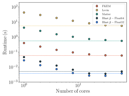
Figure 1: The impact on runtime as a function of the number of threads available on a single node. Fiducial results for 64 cores are shown as dashed horizontal lines.

As anticipated in the previous section, Blast.jl outperforms the other codes by a factor of at least $10$, which can be improved even further when working with Float32 instead of Float64. This choice does not impact the $\Delta\chi^{2}$ significantly. A breakdown of our timings is shown in Fig. 2, which indicates that the worse performance with $64$ threads is due to the evaluation of the projected matter densities $w_{\ell}$’s (defined in Eq. (24)), and also to the computation of the outer integrals to get the final $C_{\ell}$’s. The reason for such a behavior is the interaction between hyper-threading and the backends used within Blast.jl to perform the tensor contractions, as required to compute the $C_{\ell}$’s. This is not expected to be an issue, since parallelization gives almost ideal scaling up to 16 threads, and other approaches such as running more chains in parallel could be used to fully leverage the available hardware; still, we are investigating how to improve the performance when higher number of threads are employed.

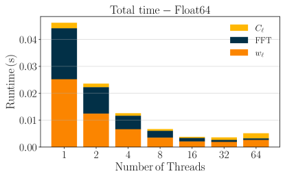
Figure 2: Breakdown of the timings for Blast.jl. The bar stacked chart shows how different part of the algorithm contribute to the total time, as a function of the number of cores employed. FFT refers to the evaluation of the Chebyshev coefficients, $w_{\ell}$ is the operation in Eq. (24), and $C_{\ell}$ refers to the computation of the two outer integrals in $\chi$-$R$, defined in Eq. (27).

6.1 Required accuracy: runtime vs max allowed $\Delta\chi^{2}$

The fiducial accuracy threshold $\Delta\chi^{2}<0.2$ imposed in the challenge has been chosen to ensure that any inaccuracies from non-Limber integration do not result in a false $1\sigma$ detection of a new effect described by a theory model. This conservative approach is designed to be robust even in the worst-case scenario, where the influence of non-Limber integration on the signal closely resembles that of the effect being mistakenly detected. In practice, it is likely that slightly less stringent accuracy requirements may be sufficient (Leonard et al., 2023). This motivated the testing of how the runtimes of the various methods scale with accuracy requirements within the range of potentially acceptable accuracy levels.

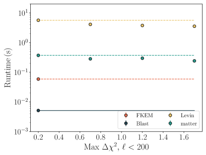
Figure 3: Run-time on 64 cores as a function of maximum allowed $\Delta\chi^{2}$ for $\ell<200$. Both Blast.jl and FKEM do not present significant runtime differences on this range of allowed $\Delta\chi^{2}$, so we present only the fiducial $\Delta\chi^{2}$ point and a horizontal line for visual comparison with other methods. The fiducial case for the other two cases is also displayed as dashed lines. Uncertainties (on the mean runtimes) are too small to be visible compared to the size of points.

As shown in Fig. 3, four different $\Delta\chi^{2}$ values were tested: $\{0.2,0.7,1.2,1.7\}$. To change Blast.jl’s accuracy, we tweaked the number of Chebyshev polynomials used for the power spectrum approximation. If for the fiducial case ($\Delta\chi^{2}<0.2$) $120$ polynomials are necessary, we can reduce them to $\lesssim 100$ if we require $\Delta\chi^{2}<1.7$. Decreasing the number of Chebyshev polynomials by such amount does not have a significant impact on the runtime, which explains why the plot only shows the fiducial case (similarly to what happens for FKEM).

6.2 Number of Spectra: Runtime vs number of tomographic bins

As in the N5K challenge, we went on to examine the scaling of the runtime with the number of auto- and cross-power spectra to be computed. To test this, the number of shear bins was fixed to $1$ (triangular markers) and $5$ (circular markers), while the number of clustering bins was varied between $1$ and $10$. Results are shown in Fig. 4. For this test, we performed $10$ benchmarks for each entry. FKEM, matter and Levin present a noticeable scaling with the number of tomographic bins. On the other hand, Blast.jl’s results are independent of the number of bins employed in the analysis. This behavior is consistent with the results from the previous section, where the number of Chebyshev polynomials in the power spectrum approximation, varied between approximately $100$ and $120$, did not have a significant impact on the runtime. Currently, the total number of bins ranges from $2$ to $15$, which, given the structure of the code, is not expected to significantly affect the computation times.

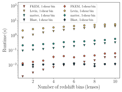
Figure 4: Timings as a function of the number of lens bins.

6.3 Width of redshift bins: $\Delta\chi^{2}$ vs bin width

The width of the tomographic redshift bins plays a crucial role in the $3\times 2$ pt analysis, as it directly affects the validity of the Limber approximation (see Sec. 2.2). Specifically, narrower bins lead to a greater breakdown of the Limber approximation, making accurate non-Limber computations increasingly important. Therefore, it is interesting to assess how our algorithm depends on that parameter. As in the N5K challenge, two new analysis scenarios were considered: in one scenario the width was reduced by a factor of $2$, in the other by a factor of $4$. Details of the new bins can be found in Leonard et al. (2023). Fig. 5 shows the result of this test: the values of $\Delta\chi^{2}$ in the three cases (full, half and quarter width) are shown for all the codes. The continuous lines connect points for which values of $\ell<200$ are considered in the evaluation of $\Delta\chi^{2}$, while the dotted lines indicate that the whole $\ell$-range is considered. As expected, the reduction of the bin size causes a lower accuracy of all methods, Blast.jl included. When using the fiducial settings, our algorithm performed in a very similar way as Levin: we observed a consistent decrease of accuracy. To improve the performance, we therefore doubled the number of sampling points in $\chi$, going from $96$ to $200$, and also increased the number of points in $R$ from $48$ to $56$. With those modifications, which match the ethos of the challenge as other entries adjusted their hyper-parameters for this test, we were able to significantly increase the accuracy, which is of the same order of magnitude as FKEM and matter. This suggests that we can push the accuracy by adding more sampling points.
The $\Delta\chi^{2}$ for the full $\ell$-range is much higher for Blast.jl than all the other codes: this is because, at this stage, we are using the first-order Limber approximation in the range $\ell\in(200,2000)$, while all of the other entries implement the more accurate second-order Limber, at least for $\ell\in(200,1000)$. Since the focus of the challenge is to compute the full integral for $\ell<200$, we did not prioritize this regime, particularly because it does not require the implementation of any new algorithm. Upon the public release of the package, higher-order Limber will be implemented for higher multipoles.

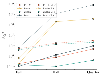
Figure 5: The impact on the accuracy for $\ell<200$ and $\ell<2000$) achieved by each integration method as a function of the width of the clustering sample bins relative to the fiducial case.

7 Conclusions

The development of accurate and fast algorithms for computing cosmological quantities is of crucial importance considering the unprecedented amount and quality of data that next-generation cosmological surveys are about to bring into the field. In this paper we focused on improving the evaluation of the model for $3\times 2$ pt statistics, without the employment of the Limber approximation. We presented Blast.jl, a new algorithm to compute non-Limber angular power spectra for galaxy clustering and cosmic shear samples, whose core idea is a decomposition of the power spectrum into the complete and orthonormal basis of the Chebyshev polynomials. By expressing the 3D matter power spectrum in terms of this basis, the most computationally challenging part of the integral can be effectively isolated, allowing for it to be pre-computed and stored. This significantly reduces the complexity of the overall computation, making it more efficient. The performance of our new algorithms was assessed in a fair and robust way, according to the standards of the N5K challenge, a non-Limber integration challenge launched in 2020 by LSST DESC (Ivezic et al., 2019) that allowed us to test Blast.jl against the state-of-the-art non-Limber algorithms. In terms of speed of computation at the required accuracy, Blast.jl outperformed FKEM, the winner of the challenge. In particular, our algorithm is $10$-$15\times$ faster in the fiducial scenario. Blast.jl runtime also proved to be basically independent of the number of tomographic redshift bins in the analysis and is also insensible to the accuracy requirements, making Blast.jl the preferred method in those scenarios. Another scaling we explored is the accuracy as a function of the width of the redshift bins: while the performance is still comparable to that of the other challenge entries, matter is still the least sensitive algorithm with respect to this specific hyper-parameter, as it keeps essentially the same accuracy when the bin width is halved. Working on improving the performance of our algorithm in this scenario is reserved for future work. Nonetheless, the tests performed in this work show that increasing the number of integration points strongly impacts Blast.jl’s accuracy, giving a possible solution to this behaviour. We also highlight that, unlike FKEM, Blast.jl does not assume a scale-independent growth factor, so it is possible to employ it in cosmologies with massive neutrinos or modified gravity scenarios. In that sense, the algorithm we really want to compare to is matter. With respect to that entry, the speed in the fiducial scenario improves by over 2 orders of magnitude. To the best of our knowledge, the fastest non-Limber integration algorithm is the one presented in this paper; actually, only the emulation of the whole $3\times 2$ pt statistic would result in a shorter runtime (Zhong et al., 2024; Saraivanov et al., 2024).

Future work will focus on adding other effects to the $C_{\ell}$’s, in particular redshift space distortions, magnification bias and relativistic corrections like the integrated Sachs-Wolfe effect. Those will enable the use of Blast.jl for a real cosmological analysis. We will also work on including the CMB as an alternative observable, allowing the user to perform galaxy-CMB lensing cross-correlation analyses. Another future development is related to the computation of the matter power spectrum; given the fast runtime of Blast.jl, it is important that this step does not become the new bottleneck of the $3\times 2$ pt computation. Currently, we are working on a matter power spectrum emulator, tailored to work in synergy with Blast.jl. Finally, Blast.jl will also include the support for automatic differentiation. Having a $3\times 2$ pt statistics code that is differentiable is crucial because it enables the use of gradient-based methods (Campagne et al., 2023; Nygaard et al., 2023; Piras et al., 2024; Bonici et al., 2024; Ruiz-Zapatero et al., 2024; Balkenhol et al., 2024; Bonici et al., 2022; Giovanetti et al., 2024). The ultimate goal is to perform cosmological parameter inference using $3\times 2$ pt statistic and a fully-differentiable likelihood that can be sampled very efficiently thanks to Blast.jl. The code will be public upon acceptance of this paper.

Appendix A Choosing an effective basis for the integration

A crucial step for the successful calculation of the angular power spectra with this method is the re-parametrization of the integral from the $\chi_{1}$-$\chi_{2}$ variables to $\chi$-$R$, with $R\equiv\chi_{2}/\chi_{1}$. The projected matter densities (Eq. (24)) present a sharp feature along their diagonal ($\chi_{1}=\chi_{2}$). Capturing this feature in the $\chi_{1}$-$\chi_{2}$ reference frame would require a high number of sampling points ($>>500$), which is computationally not convenient. If we define $R$ as the ratio of the coordinates, we know that $R\in(0,1]$, and $R=1$ represents the diagonal. It is therefore easier and more intuitive to perform a finer sampling of the diagonal feature, and a coarser one outside the diagonal, where the contribution to the integral are close to zero. Fig. 6 is a visual representation of this change of basis, showing how most of the contributions to the integral come from $R>0.8$. Note also that the figure shows a low multipole $\ell=2$, for which the off-diagonal contributions are still relevant. For higher multipole orders, the feature gets sharper and sharper. This effectively shows why the Limber approximation, which accounts only for the contribution coming from the diagonal $\chi_{1}=\chi_{2}$, is more accurate at higher multipoles $\ell$.

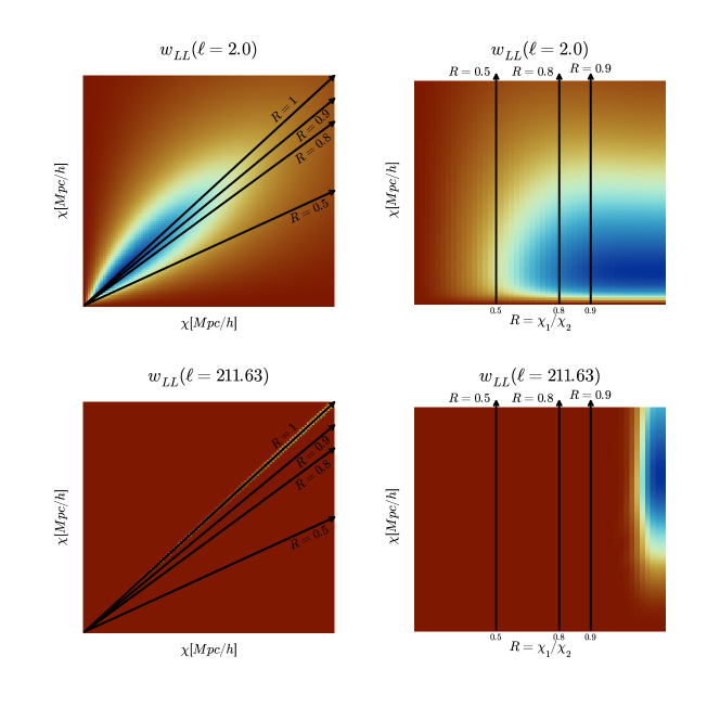
Figure 6: Visual representation of the change of the re-parametrization of the projected matter density (Eq. (24)) from coordinates $\chi_{1}$-$\chi_{2}$ to $\chi$-$R$. The heatmaps represent $w^{ss}(\ell=2.0)$ and $w^{ss}(\ell=211.63)$ in the two different coordinate systems. The image shows how defining the coordinate R allows for a better description of the object, especially for higher multipole orders. The matrices are normalized to their maximum value, so the color scheme goes from $-1$ (dark red) to $1$ (blue).

The full calculation for the change of variables will now be worked out. The first step consists in noting that the integral can be symmetrized:

$$C_{ij}^{\mathrm{AB}}(\ell) =\int_{0}^{\infty}d\chi_{1}K_{i}^{\mathrm{A}}(\chi_{1})\int_{0}^{\infty}d\chi_{2}K_{j}^{\mathrm{B}}(\chi_{2})w_{\mathrm{AB}}(\chi_{1},\chi_{2})=$$ (36)

$$=\int_{0}^{\infty}d\chi_{1}K_{i}^{\mathrm{A}}(\chi_{1})\int_{0}^{\chi_{1}}d\chi_{2}K_{j}^{\mathrm{B}}(\chi_{2})w_{\mathrm{AB}}(\chi_{1},\chi_{2})+\int_{0}^{\infty}d\chi_{2}K_{j}^{\mathrm{B}}(\chi_{2})\int_{0}^{\chi_{2}}d\chi_{1}K_{i}^{\mathrm{A}}(\chi_{1})w_{\mathrm{AB}}(\chi_{2},\chi_{1}).$$

In the first integral, the change of variable is $R=\chi_{2}/\chi_{1}$, in the second one $R=\chi_{1}/\chi_{2}$. Adding that into Eq. (36), one finds:

$$C_{ij}^{\mathrm{AB}}(\ell) =\int_{0}^{\infty}d\chi\int_{0}^{1}dR\chi\left[\mathcal{K}_{i}^{\mathrm{A}}(\chi)\mathcal{K}_{j}^{\mathrm{B}}(R\chi)+\mathcal{K}_{j}^{\mathrm{B}}(\chi)\mathcal{K}_{i}^{\mathrm{A}}(R\chi)\right]w_{\mathrm{AB}}(\chi,R\chi)$$ (37)

$$=\int_{0}^{\infty}d\chi\int_{0}^{1}dR\chi\tilde{\mathcal{K}}_{ij}^{\mathrm{AB}}(\chi,R\chi)w_{\mathrm{AB}}(\chi,R\chi),$$

where:

$$\mathcal{K}_{i}^{\mathrm{A}}(\chi)=\begin{cases}K_{i}^{\mathrm{A}}(\chi)&\text{for clustering}\\ K_{i}^{\mathrm{A}}(\chi)/\chi^{2}&\text{for lensing}\end{cases}$$ (38)

Appendix B Assessing model errors

The following plots show the errors with respect to the benchmarks, expressed as a fraction of the cosmic variance (the Gaussian statistical uncertainties), defined by the Knox’s formula (Knox, 1995):

$$\sigma_{ij}^{\mathrm{AB}}(\ell)=\sqrt{\frac{C_{ii}^{\mathrm{AA}}(\ell)C_{jj}^{\mathrm{BB}}(\ell)+(C_{ij}^{\mathrm{AB}}(\ell))^{2}}{f_{\text{sky}}(2\ell+1)}}$$ (39)

where we are using $f_{\text{sky}}=0.4$, the sky fraction for LSST. In particular, we can define a metric that is often referred to as Mean Absolute Error Ratio (MAER):

$$\text{MAER}^{\mathrm{AB}}_{ij}(\ell)=\frac{|C_{ij}^{\mathrm{AB}}(\ell)-C_{ij,\text{bench}}^{\mathrm{AB}}(\ell)|}{\sigma_{ij}^{\mathrm{AB}}(\ell)}$$ (40)

Fig. 7-9 show the quantity $\Delta C_{\ell}/\sigma_{\ell}$, defined as the MAER in Eq. (40), for the auto- and cross- correlations between $5$ of the clustering and shear redshift bins for the Limber approximation, the three entries of the challenge and Blast.jl. As discussed in Sec. 2.2, the Limber approximation is not accurate for small $\ell$, where the error is at a level of $\approx 10\%$. All the non-Limber methods, Blast.jl included, are able to reduce the error on those scales. In particular, the error given by our implementation is compatible to that of the other codes, and is very stable across the whole range of $\ell$ and the different bin combinations. This is very positive as spikes in $\Delta C_{\ell}/\sigma$ can have a strong impact on the $\Delta\chi^{2}$. For $\ell>200$, the errors are comparable to the Limber: most implementations, ours included, actually use the approximation for higher multipole orders. Finally, we discussed how the Limber approximation is more accurate for the shear-shear auto-correlation because the weak lensing kernels cover a wide range of $\chi$ values: this explains why the improvement given by all non-Limber methods is way less drastic in that case (Fig. 9).

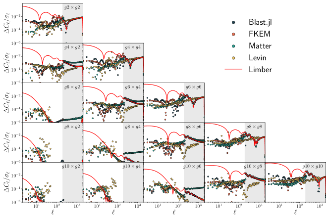
Figure 7: Deviation with respect to the benchmarks in the different auto- and cross-correlations between five of the clustering redshift bins (identified as $g$) used in this analysis as a fraction of the Gaussian uncertainties. Results are shown for the pure Limber approximation (red), Blast (blue), FKEM (orange), Levin (yellow), and matter (turquoise). The grey band represents the region where $\ell>200$, not part of the challenge set-up. This figure visually shows how the goal of improving with respect to the Limber approximation is accomplished. Moreover, the error of our algorithm are comparable to the other challenge entries.

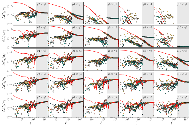
Figure 8: Same as Figure 7 for the clustering-shear cross-correlations (in the same clustering bins). The shear bins are identified as $\gamma$, while $g$ is used for the galaxy clustering tomographic bins.

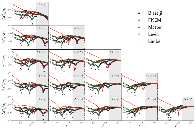
Figure 9: Same as Figure 7 for the shear-shear auto- and cross-correlations.

Appendix C Pre-computation efficiency

The core idea of the algorithm is to pre-compute the cosmology-independent quantities defined in Eq. (24). As discussed in Sec. 3.2, we performed the integrals using the Clenshaw-Curtis integration rule and $N=2^{15}+1$ points in the interval $[k_{\mathrm{min}},k_{\mathrm{max}}]$. The following plot motivates the choice of the parameter $N$ by showing its impact on the accuracy, i.e., the $\Delta\chi^{2}$.

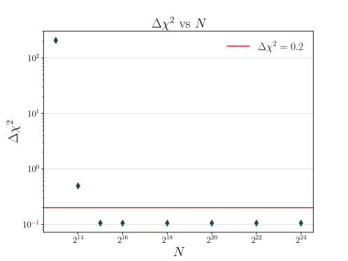
Figure 10: Accuracy as a function of the number of integration points used to evaluate the integrals in Eq. (24). The plot shows that our algorithm is well converged for $N>2^{15}$. The red line indicates the accuracy requirement from the N5K challenge.

References

- Balkenhol et al. (2024) Balkenhol L., Trendafilova C., Benabed K., Galli S., 2024, Astronomy & Astrophysics, 686, A10
- Bonici et al. (2022) Bonici M., Biggio L., Carbone C., Guzzo L., 2022, Fast emulation of two-point angular statistics for photometric galaxy surveys (arXiv:2206.14208), https://arxiv.org/abs/2206.14208
- Bonici et al. (2024) Bonici M., Baxter E., Bianchini F., Ruiz-Zapatero J., 2024, The Open Journal of Astrophysics, 7
- Campagne et al. (2017) Campagne J.-E., Neveu J., Plaszczynski S., 2017, Astronomy & Astrophysics, 602, A72
- Campagne et al. (2023) Campagne J.-E., et al., 2023, The Open Journal of Astrophysics, 6
- Carron (2013) Carron J., 2013, Astronomy & Astrophysics, 551, A88
- Chisari & Pontzen (2019) Chisari N. E., Pontzen A., 2019, Physical Review D, 100, 023543
- Clenshaw & Curtis (1960) Clenshaw C. W., Curtis A. R., 1960, Numerische Mathematik, 2, 197
- Fang et al. (2020) Fang X., Krause E., Eifler T., MacCrann N., 2020, Journal of Cosmology and Astroparticle Physics, 2020, 010
- Feldbrugge (2023) Feldbrugge J., 2023, Complex evaluation of angular power spectra: Going beyond the Limber approximation (arXiv:2304.13064), https://arxiv.org/abs/2304.13064
- Frigo & Johnson (1997) Frigo M., Johnson S. G., 1997, The fastest fourier transform in the west
- Giovanetti et al. (2024) Giovanetti C., Lisanti M., Liu H., Mishra-Sharma S., Ruderman J. T., 2024, arXiv preprint arXiv:2408.14538
- Grasshorn Gebhardt & Jeong (2018) Grasshorn Gebhardt H. S., Jeong D., 2018, Physical Review D, 97, 023504
- Hamilton (2000) Hamilton A., 2000, Monthly Notices of the Royal Astronomical Society, 312, 257
- Hamimeche & Lewis (2008) Hamimeche S., Lewis A., 2008, Physical Review D—Particles, Fields, Gravitation, and Cosmology, 77, 103013
- Hu & White (1997) Hu W., White M., 1997, Physical Review D, 56, 596
- Ivezic et al. (2019) Ivezic Z., et al., 2019, The Astrophysical Journal, 873, 111
- Knox (1995) Knox L., 1995, Physical Review D, 52, 4307
- Leonard et al. (2023) Leonard C. D., et al., 2023, The Open Journal of Astrophysics, 6
- Levi et al. (2019) Levi M. E., et al., 2019, The Bulletin of the American Astronomical Society, 57
- Levin (1996) Levin D., 1996, Journal of Computational and Applied Mathematics, 67, 95
- Limber (1953) Limber D. N., 1953, PhD thesis, The University of Chicago
- LoVerde & Afshordi (2008) LoVerde M., Afshordi N., 2008, Physical Review D—Particles, Fields, Gravitation, and Cosmology, 78, 123506
- Mellier et al. (2024) Mellier Y., et al., 2024, Euclid. I. Overview of the Euclid mission (arXiv:2405.13491), https://arxiv.org/abs/2405.13491
- Nygaard et al. (2023) Nygaard A., Holm E. B., Hannestad S., Tram T., 2023, Journal of Cosmology and Astroparticle Physics, 2023, 064
- Piras et al. (2024) Piras D., Polanska A., Mancini A. S., Price M. A., McEwen J. D., 2024, The Open Journal of Astrophysics, 7
- Press (2007) Press W. H., 2007, Numerical recipes 3rd edition: The art of scientific computing. Cambridge university press
- Ruiz-Zapatero et al. (2024) Ruiz-Zapatero J., Alonso D., García-García C., Nicola A., Mootoovaloo A., Sullivan J. M., Bonici M., Ferreira P. G., 2024, The Open Journal of Astrophysics, 7
- Saraivanov et al. (2024) Saraivanov E., Zhong K., Miranda V., Boruah S. S., Eifler T., Krause E., 2024, Attention-Based Neural Network Emulators for Multi-Probe Data Vectors Part II: Assessing Tension Metrics (arXiv:2403.12337)
- Schöneberg et al. (2018) Schöneberg N., Simonović M., Lesgourgues J., Zaldarriaga M., 2018, Journal of Cosmology and Astroparticle Physics, 2018, 047
- Talman (1978) Talman J. D., 1978, Journal of computational physics, 29, 35
- Trefethen (2019) Trefethen L. N., 2019, Approximation theory and approximation practice, extended edition. SIAM
- Wang et al. (2022) Wang Y., et al., 2022, The Astrophysical Journal, 928, 1
- Zhong et al. (2024) Zhong K., Saraivanov E., Caputi J., Miranda V., Boruah S. S., Eifler T., Krause E., 2024, Attention-based Neural Network Emulators for Multi-Probe Data Vectors Part I: Forecasting the Growth-Geometry split (arXiv:2402.17716)
- de la Bella et al. (2021) de la Bella L. F., Tessore N., Bridle S., 2021, JCAP, 08, 001