Abstract

The Hamiltonian Monte Carlo (HMC) algorithm is often lauded for its ability to effectively sample from high-dimensional distributions. In this paper we challenge the presumed domination of HMC for the Bayesian analysis of GLMs. By utilizing the structure of the compute graph rather than the graphical model, we reduce the time per sweep of a full-scan Gibbs sampler from $O(d^{2})$ to $O(d)$, where $d$ is the number of GLM parameters. Our simple changes to the implementation of the Gibbs sampler allow us to perform Bayesian inference on high-dimensional GLMs that are practically infeasible with traditional Gibbs sampler implementations. We empirically demonstrate a substantial increase in effective sample size per time when comparing our Gibbs algorithms to state-of-the-art HMC algorithms. While Gibbs is superior in terms of dimension scaling, neither Gibbs nor HMC dominate the other: we provide numerical and theoretical evidence that HMC retains an edge in certain circumstances thanks to its advantageous condition number scaling. Interestingly, for GLMs of fixed data size, we observe that increasing dimensionality can stabilize or even decrease condition number, shedding light on the empirical advantage of our efficient Gibbs sampler.

1 Introduction

Figure 1: Part of a GLM compute graph with three regression parameters. In the figure we compute $\ell_{i}$, the log-likelihood corresponding to data point $i$. Using caching techniques we reduce the complexity of Gibbs from $O(d^{2})$ to $O(d)$. Our set of regression parameters after a coordinate update on $j=2$ with a Gibbs sampler is $\theta^{\prime}=(\theta_{1},\theta_{2}^{\prime},\theta_{3})$. To recompute $\ell_{i}$ after updating $\theta^{\prime}_{2}$, we only need to modify the entries highlighted in red. Using caches updated by subtracting the old value and adding the new one at the ‘$+$’ node, this change can be performed in $O(1)$ operations, instead of $O(d)$ operations. Over $d$ coordinates, Gibbs then has a cost of $O(d)$ instead of $O(d^{2})$.

Generalized linear models (GLMs) are among the most commonly used tools in contemporary Bayesian statistics [13]. As a result, applied Bayesian statisticians require efficient algorithms to approximate the posterior distributions associated with GLM parameters, often relying on Markov chain Monte Carlo (MCMC). In this paper we focus on two MCMC samplers: the Gibbs sampler and Hamiltonian Monte Carlo (HMC), popularized in statistics by [14] and [30], respectively.

Until around 2010, Gibbs sampling was the predominant option, as it formed the core of a “first generation” of probabilistic programming languages (PPLs) such as BUGS [28] and JAGS [34]. A large shift occurred in the early 2010s when HMC and its variant, the No U-Turn Sampler (NUTS) [20], were combined with reverse-mode automatic differentiation [29] to power a “second generation” of PPLs such as Stan [8]. Subsequently, HMC largely replaced Gibbs as the focus of attention of the methodological, theoretical, and applied MCMC communities. (A notable exception is Gibbs sampling under specific linear and conditionally Gaussian models [33, 47].)

Our first contribution is an algorithm for Gibbs sampling of GLMs that speeds up inference by a factor $O(d)$, where $d$ is the number of parameters, compared to the Gibbs implementation used by “first generation” PPLs. The main idea behind this speedup is to use information encoded in the compute graph associated with the target log density—in contrast, previous Gibbs algorithms relied on graphical models [22], which we show is a sub-optimal representation of GLMs for the purpose of efficient Gibbs sampling. The compute graph is a directed acyclic graph (DAG) encoding the dependencies between the operations involved in computing a function. See Figure 1 for an example. Programming strategies to extract and manipulate such graphs are well developed, in large part because compute graphs also play a key role in reverse-mode automatic differentiation [29].

This drastic $O(d)$ speedup prompted us to reconsider if Gibbs sampling should be reappraised as a method of choice for approximating GLM posterior distributions. A holistic comparison of sampling algorithms requires taking into account not only the running time per iteration, but also the number of iterations to achieve one effective sample. To understand the latter, we use a combination of empirical results and theory. On the theoretical side, we consider normal models, where both HMC and Gibbs have well-developed results quantifying the number of iterations needed to achieve one effective sample [38, 7, 10]. In this setting, the $O(d)$ runtime of our improved Gibbs sampler combined with past theory yields a favourable $O(d)$ floating point operations (flops) per effective sample, compared with the higher $O(d^{5/4})$ flops per effective sample for HMC. While the $d^{1/4}$ advantage of Gibbs over HMC may seem minor, a key point is that Gibbs requires no adaptation to achieve this performance, while HMC needs to be finely tuned adaptively [27], implying that the practical rate for HMC may be even higher. Note also that previous, graphical model-based implementations of Gibbs sampling require $O(d^{2})$ flops per effective sample in the same setup. Although these results pertain only to normal models, the theory of Gibbs and HMC is not yet mature enough for a more general comparison. Existing analyses of Gibbs sampling are model-specific [6, 4] or do not take into account scaling with respect to both condition number and dimension [43, 44, 45, 46], and the scaling of randomized or dynamic HMC as a function of the condition number is still an open problem as of the time of writing. In this work, we avoid the fallacy of comparing algorithms via loose complexity upper bounds. See Section 4 for an extensive discussion and bibliography.

Examining scaling in $d$ alone does not provide a full story, even in the normal setting; the shape of the posterior contour lines also has a strong effect on the sampling performance of both Gibbs and HMC. Various notions of condition number $\kappa$ are used [24, 19] to summarize the complexity brought by the shape of log-concave distributions. In gradient-based methods, a popular notion of condition number is the square of the broadest direction’s scale to that of the most constrained. For optimally-tuned HMC with non-constant integration time on Gaussian targets, the cost per effective sample is $O(d^{5/4}\kappa^{1/2})$ flops [24, 3, 42, 21]. Understanding the condition number scaling of Gibbs is more nuanced, as Gibbs sampling is invariant to axis-aligned stretching [39], but is sensitive to rotations (the situation is reversed for HMC [32]). We develop a notion of residual condition number, $\kappa_{\text{res}}$, to capture how Gibbs perceives the target’s shape. Crucially, $\kappa_{\text{res}}\leq\kappa$. On the other hand, due to random walk behaviour, Gibbs’ cost per effective sample scales as $O(d\kappa_{\text{res}})$ flops, and in some cases, $\kappa=\kappa_{\text{res}}$, leading to a potentially worst or better scaling in the condition number for Gibbs compared to HMC, depending on the nature of the target. As a result, neither Gibbs sampling nor HMC dominate each other.

The relative importance of $\kappa$ and $d$ will in general be problem-dependent. To get some insight on how these quantities relate to each other in practice, we investigate sequences of posterior distributions obtained by subsampling an increasing number of covariates from real datasets. We find that various notions of condition number increase until $d\approx n$, after which they either stabilize or, surprisingly, can in certain cases decrease with $d$. This suggests that our efficient Gibbs sampling will be particularly effective in GLMs where $d\gg n$.

We implemented our new Gibbs algorithm and benchmarked it using a collection of synthetic and real datasets. In 7 out of the 8 datasets considered, our algorithm achieves a higher effective sample size (ESS) per second compared to Stan, with a speed-up of up to a factor of 300.

The paper is organized as follows. In Section 2 we provide a review of some key concepts such as Gibbs sampling, Hamiltonian Monte Carlo, and GLMs. We then present our compute graph-based approach to Gibbs sampling for GLMs in Section 3. Theoretical results concerning the convergence rate of Gibbs samplers and HMC are presented in Section 4. In Section 5 we present numerical results on real and synthetic data sets to gain further insight on the performance of our Gibbs algorithm compared to state-of-the-art HMC algorithms.

2 Background

In this section we introduce several key concepts for studying the Gibbs sampler and HMC when applied to GLMs. Throughout this paper, we denote the target distribution of interest on $\mathbb{R}^{d}$ by $\pi$, with density

$$\pi(\theta)\propto e^{-U(\theta)},\quad\theta\in\mathbb{R}^{d},$$ (2)

with respect to Lebesgue measure on $\mathbb{R}^{d}$. We assume that for all $\theta\in\mathbb{R}^{d}$, $\nabla U(\theta)$ and $\nabla^{2}U(\theta)$ are well-defined. The distribution $\pi$ is called strongly log-concave if there exists a constant $a>0$ such that for all $\theta\in\mathbb{R}^{d}$, $\nabla^{2}U(\theta)\succeq aI_{d}$, and strongly log-smooth if there exists a constant $b>0$ such that for all $\theta\in\mathbb{R}^{d}$, $\|\nabla^{2}U(\theta)\|\leq b<\infty$.

2.1 Gibbs sampling

In this paper we use the term “Gibbs sampler” to refer to a general class of algorithms sometimes also referred to as “(Metropolis-)within-Gibbs” [12]. In the literature, the term “Gibbs sampler” is associated with two key ideas: (1) moving a subset of coordinates while fixing the others; and (2), using the conditional distribution of the target distribution to perform such an update. The algorithm in Section 3 is described for simplicity in the context of Gibbs samplers, but applies more generally to any “within-Gibbs” sampler. In the experiments, we use “slice sampling within Gibbs”, specifically, with doubling and shrinking [31]. See Section 4.3 for more discussion on Gibbs versus “within-Gibbs.”

For $\theta=(\theta_{1},\ldots,\theta_{d})$ and $j\in\{1,2,\ldots,d\}$, let $\theta_{-j}$ be the vector containing all components of $\theta$ except for $\theta_{j}$. We define the conditional distributions $\pi_{j|-j}$, which correspond to the conditional distributions of $\theta_{j}$ given $\theta_{-j}$, where $\theta\sim\pi$. In Metropolis-within-Gibbs, each coordinate is performed using a Markov kernel $K_{j|-j}$ that leaves $\pi_{j|-j}$ invariant. The idealized Gibbs sampler uses the Markov kernels $K_{j|-j}(x,\cdot)=\pi_{j|-j}(\cdot)$, but more general kernels are commonly used as well [31]. It remains to decide the order in which to update coordinates. One popular approach is to use a deterministic update Gibbs sampler (DUGS) [38, 16], where coordinates are updated in a fixed order. For example, when $d=3$, the DUGS kernel is:

$$\theta_{1}^{\prime} \sim K_{1|-1}(\cdot|\theta_{2},\theta_{3}),$$ (3)

$$\theta_{2}^{\prime} \sim K_{2|-2}(\cdot|\theta_{1}^{\prime},\theta_{3}),$$ (4)

$$\theta_{3}^{\prime} \sim K_{3|-3}(\cdot|\theta_{1}^{\prime},\theta_{2}^{\prime}).$$ (5)

We write $K_{\text{DUGS}}$ for the idealized DUGS Markov kernel with $K_{j|-j}(x,\cdot)=\pi_{j|-j}(\cdot)$, where one kernel step performs an update on all $d$ coordinates. Options beyond DUGS are the random scan Gibbs sampler, which chooses coordinates to update randomly, and collapsed Gibbs samplers, which chooses several coordinates to update at once and can improve convergence [26]. In this work, we focus primarily on $K_{\text{DUGS}}$, as it yields a smaller asymptotic variance than random scan Gibbs in some problem classes [16, 35, 2]—although a definitive conclusion is more nuanced [37, 18]—and because updating only one coordinate at a time enables a clear analysis of the relationship between $d$ and convergence.

2.2 Hamiltonian Monte Carlo

Hamiltonian Monte Carlo (HMC) is an MCMC algorithm that makes use of gradient information of the target density and introduces a momentum in the sampling process to provide efficient exploration of the state space [32]. Calculating the trajectory of HMC samples requires solving a differential equation, which is approximated using numerical integrators in practice. We introduce HMC in two phases: using idealized trajectories, which assume that exact numerical integrators exists; and with the leapfrog integrator, a popular numerical integrator in the case of HMC. In both cases, the HMC kernel has an invariant distribution on an augmented space with momentum variables $p\in\mathbb{R}^{d}$, with joint density

$$\bar{\pi}(\theta,p)=\pi(\theta)\cdot\mathcal{N}(p\mid 0,M),$$ (6)

which admits $\pi$ as the $\theta$-marginal. Here, $M$ is the covariance matrix of the Gaussian momentum, which is often referred to as the mass matrix of HMC. In practice, $M$ is often restricted to be diagonal.

For idealized HMC, we initialize with a starting point $\theta^{(0)}=\theta(0)$ at time $t=0$ and some momentum $p(0)\sim\mathcal{N}(0,M)$. We specify a (possibly random) integration time $\tau$ and solve for $\{\theta(t)\}_{t\in[0,\tau]}$ from

$$\theta^{\prime}(t)=M^{-1}\cdot p(t),\qquad p^{\prime}(t)=-\nabla U(\theta(t)),$$ (7)

which corresponds to Hamiltonian dynamics. We then record the draw $\theta^{(1)}\leftarrow\theta(\tau)$, reset $\theta(0)\leftarrow\theta(\tau)$, and draw a new $p(0)\sim\mathcal{N}(0,M)$. Repeating the process, we obtain a sequence of draws $\theta^{(0)},\theta^{(1)},\theta^{(2)},\ldots$.

It is not generally possible to simulate the trajectory in Eq. 7 exactly, so numerical integration is used. For a given starting point $(\theta,p)$, integration step size $\epsilon>0$, and number of steps $s$, the leapfrog $L_{\epsilon}$ [32] is applied $s$ times, where $\theta^{\prime},p^{\prime}=L_{\epsilon}(\theta,p)$ is defined by

$$p^{\prime}_{\nicefrac{{1}}{{2}}} =p-\frac{\epsilon}{2}\nabla U(\theta),$$ (8)

$$\theta^{\prime} =\theta+\epsilon M^{-1}\cdot p^{\prime}_{\nicefrac{{1}}{{2}}},$$ (9)

$$p^{\prime} =p^{\prime}_{\nicefrac{{1}}{{2}}}-\frac{\epsilon}{2}\nabla U(\theta^{\prime}).$$ (10)

Applying $L_{\epsilon}^{s}(\theta,p)$ ($L_{\epsilon}$ applied $s$ times to $(\theta,p)$) we obtain a proposed point $({\widetilde{\theta}},{\widetilde{p}})$ that approximates the idealized HMC point $(\theta(\tau),p(\tau))$ at time $\tau=\epsilon s$. A Metropolis–Hastings (MH) accept-reject step is then introduced in order to leave $\bar{\pi}$ invariant; the proposal $({\widetilde{\theta}},{\widetilde{p}})$ is accepted with probability

$$\alpha((\theta,p),({\widetilde{\theta}},{\widetilde{p}}))=\left\{1,\frac{\exp(-U({\widetilde{\theta}}))\mathcal{N}({\widetilde{p}}\mid 0,M)}{\exp(-U(\theta))\mathcal{N}(p\mid 0,M)}\right\},$$ (11)

and otherwise we remain at $(\theta,p)$.

2.3 Generalized linear models

Suppose we are given $n$ observations $\{(x_{i},y_{i})\}_{i=1}^{n}$ with fixed covariates $x_{i}\in\mathbb{R}^{d}$ and observations $y_{i}\in{\mathcal{Y}}\subset\mathbb{R}$ of independent random responses $Y_{i}$. The independent random responses $Y_{i}$ are modelled as coming from a certain conditional distribution $f_{Y|X}$, which we assume has a density with respect to some common dominating measure for any given $x$. We parametrize this density in terms of the mean of the distribution; in a generalized linear model (GLM), the mean of the distribution of response $Y_{i}$ is assumed to depend only on the linear predictor $x_{i}^{\top}\theta$, where $\theta\in\mathbb{R}^{d}$. We fix some inverse link function, $\mu$, and model the mean

$$\mathbb{E}[Y_{i}]=\mu(x_{i}^{\top}\theta)\equiv\mu_{i}.$$ (12)

The full likelihood is then

$${\mathcal{L}}(\theta)=\prod_{i=1}^{n}f_{Y|X}(y_{i}\mid\mu_{i}),$$ (13)

and the log-likelihood corresponding to data point $(x_{i},y_{i})$ is $\ell_{i}=\log f_{Y|X}(y_{i}\mid\mu_{i})$. In the Bayesian framework, a prior with density $\pi_{0}$ is specified on the regression parameters, such that one obtains a posterior distribution with density

$$\pi(\theta)\propto\pi_{0}(\theta)\cdot{\mathcal{L}}(\theta).$$ (14)

2.4 Condition numbers and preconditioning

The condition number of a given positive definite matrix $M$ is defined as $\kappa(M):=\lambda_{\text{max}}(M)/\lambda_{\text{min}}(M)$ where $\lambda_{\text{max}}(M)$ and $\lambda_{\text{min}}(M)$ are the largest and smallest eigenvalues of $M$, respectively. We can generalize this definition to accommodate strongly log-concave distributions. For a strongly log-concave distribution $\pi$, the condition number of $\pi$ can be defined as:

$$\kappa(\pi):=\sup_{\theta\in\mathbb{R}^{d}}\left\|\nabla^{2}U(\theta)\right\|\sup_{\theta\in\mathbb{R}^{d}}\left\|\nabla^{2}U(\theta)^{-1}\right\|.$$ (15)

In particular, when $\pi$ is Gaussian $\mathcal{N}(\mu,\Sigma)$, we have $\kappa(\pi)=\kappa(\Sigma)=\lambda_{\text{max}}(\Sigma)/\lambda_{\text{min}}(\Sigma)$. Moving forward, we refer to $\kappa(\pi)$ as the raw condition number; we simply denote this $\kappa$ when there is no ambiguity about the target distribution.

It is common to transform the target distribution $\pi$ with a preconditioning matrix $A$ in order to try to reduce the condition number. That is, given $\theta\sim\pi$ and a full rank $d$ by $d$ matrix $A$, we define $\pi_{A}$ such that $\theta_{A}=A\theta\sim\pi_{A}$. In the context of HMC, preconditioning with $A$ is equivalent to setting the mass matrix to $A^{\top}A$ [19]. One common approach to preconditioning is to set

$$A=\operatorname{diag}(\operatorname{Var}_{\pi}[\theta_{j}]^{-1/2}).$$ (16)

In this case, we refer to $\kappa(\pi_{A})$ as the correlation condition number, denoted as $\kappa_{\mathrm{cor}}(\pi)$, since the covariance and correlation matrix of $\pi_{A}$ are the same. It is often implicitly assumed that $\kappa_{\mathrm{cor}}\leq\kappa$, but this is not always true [19], as we also see in our experiments.

We finally introduce the notion of the residual condition number, $\kappa_{\mathrm{r}}(\pi)$, which is defined as

$$\kappa_{\mathrm{r}}(\pi):=\inf_{A\in\mathcal{D}}\kappa(\pi_{A}),$$ (17)

where $\mathcal{D}$ is the set of full rank $d\times d$ diagonal matrices with positive entries. By definition, $\kappa_{\mathrm{r}}\leq\kappa$. We will demonstrate in Section 4 that the convergence rate for Gibbs sampling depends on $\kappa_{\mathrm{r}}$, as opposed to $\kappa$.

3 Fast Gibbs sampling for GLMs

In this section we present our approach to Gibbs sampling for GLMs that reduces the computation time for full-scan Metropolis–Hastings updates from $O(d^{2}n)$ to $O(dn)$. This is achieved by studying the compute graph of a GLM, a directed graph that describes the order of operations for computing the posterior density of the model. We perform our optimizations using simple caching techniques.

To illustrate our technique, we turn to logistic regression with parameters $\theta=(\theta_{1},\ldots,\theta_{d})$ and data points $\{(x_{i},y_{i})\}_{i=1}^{n}$. The likelihood for this model is given by

$${\mathcal{L}}(\theta) =\prod_{i=1}^{n}p_{i}(\theta)^{y_{i}}(1-p_{i}(\theta))^{1-y_{i}},$$ (18)

$$p_{i}(\theta) =\frac{1}{1+\exp\left(-x_{i}^{\top}\theta\right)}.$$ (19)

We now introduce a flavour of compute graph suitable for our purpose, namely a type of directed graph associated with a function $f(\theta_{1},\dots,\theta_{d})$—see Fig. 1 for an example in the GLM context. First, for each variable $\theta_{j}$, we assume there is a corresponding input node in the graph such that no edge points into it. We call the graph vertices that are not input nodes the compute nodes. For each compute node $n$, we assume there is an associated operation, i.e., a function that takes as input the values given by the nodes $n^{\prime}$ such that $(n^{\prime}\to n)$ is an edge in the graph. We assume the compute graph has a single sink node, i.e., a node which has no outgoing edge. We assume the compute graph is such that the composition of the operations along the graph from inputs to sink is identical to $f(\theta_{1},\dots,\theta_{d})$.

In Fig. 1, we see that the part of the compute graph for calculating the likelihood associated with data point $x_{i}$ revolves around computing the term $x_{i}^{\top}\theta$. After a single-coordinate update of $\theta$, as would be done with the Gibbs sampler, many of the calculations carry over (the new ones are highlighted in red). This simple observation is the key to our $O(d)$ speedup of the Gibbs sampler for GLMs.

We now introduce our approach for computing the likelihood of GLMs, which we call compute graph Gibbs (CGGibbs). This approach is based on the following idea: cache the scalar values of the linear predictors $x_{i}^{\top}\theta$ for each data point $i$ in a vector, cache. This requires only $O(n)$ memory (this is negligible since the design matrix already requires storing $d\cdot n$ entries), but yields an $O(d)$ computational speedup. This approach is possible because the Gibbs sampler considers coordinate-wise updates of the form $\theta=(\theta_{1},\ldots,\theta_{j},\ldots,\theta_{d})\mapsto\theta^{\prime}=(\theta_{1},\ldots,\theta^{\prime}_{j},\ldots,\theta_{d})$, and consequently likelihood updates have a special structure. For such updates, we have the convenient decomposition

$$x_{i}^{\top}\theta^{\prime} =\sum_{j=1}^{d}\theta_{j}^{\prime}x_{ij}$$ (20)

$$=\sum_{j=1}^{d}\theta_{j}x_{ij}-\theta_{j}x_{ij}+\theta_{j}^{\prime}x_{ij}$$ (21)

$$=\texttt{cache}[i]-\theta_{j}x_{ij}+\theta_{j}^{\prime}x_{ij}.$$ (22)

This new linear predictor for a given data point can be computed in $O(1)$ time with caching, compared to $O(d)$ time without caching. From here, one evaluation of the full likelihood comes at an $O(n)$ cost, and a full sweep over $d$ coordinates is thus an $O(dn)$ cost, instead of the usual $O(d^{2}n)$ that would be incurred without caching. The resulting speedup in terms of the number of parameters, $d$, allows us to apply this new approach to Bayesian inference with Gibbs sampling to high-dimensional regression problems, including ones where $d\gg n$.

Although this simple optimization is obvious from the compute graph, presented in Fig. 1, it is not obvious from the graphical model corresponding to the given regression problem in Fig. 2. Probabilistic programming languages (PPLs) incorporating Gibbs samplers often perform optimizations in evaluating ratios of likelihoods for Markov kernel proposals with respect to graphical models, such as the one in Fig. 2. However, these graphs only reveal the dependence structure of random variables in the model and decompositions of the likelihood, but they do not yield insight into fine-grained optimization of computations such as in Fig. 1. In our case, this “fine-grained” optimization yields a substantial $O(d)$ improvement in computation time with the introduction of simple caching techniques.

Figure 2: A directed acyclic graph (DAG) for a regression problem with five data points $(x_{i},Y_{i})$ and three regression parameters $\theta_{j}$. Only edges into $Y_{3}$ are emphasized and the covariates $x_{i}$ are assumed fixed. Observed variables are shaded in gray. Compared to Fig. 1, fewer information is available as to how $\theta$ and $Y_{i}$ are related.

4 Theory

We begin by comparing the convergence rates of idealized DUGS and HMC in Section 4.1, focusing on how the convergence rate of each sampling algorithm scales with respect to the dimension $d$ and condition number $\kappa$ of the target distribution. In Section 4.2 we discuss the practical implications of our convergence analysis and the influence of linear preconditioning on the convergence rates of both algorithms.

4.1 Convergence rates and scaling

We review the current literature and present new results on the convergence rate of idealized Gibbs and HMC with respect to various divergences. Let $\pi_{1},\pi_{2}$ be given distributions and let $\mathcal{C}(\pi_{1},\pi_{2})$ be the set of all couplings of $\pi_{1}$ and $\pi_{2}$ (joint distributions admitting $\pi_{1}$ and $\pi_{2}$ as marginals). The divergences used in these works include the total variation ($\operatorname{TV}$) distance

$$\operatorname{TV}(\pi_{1},\pi_{2})=\inf_{(X,Y)\in\mathcal{C}(\pi_{1},\pi_{2})}\mathbb{P}(X\neq Y),$$ (23)

the $p$-Wasserstein ($\mathrm{W}_{p}$) distance

$$\mathrm{W}_{p}(\pi_{1},\pi_{2})=\left(\inf_{(X,Y)\in\mathcal{C}(\pi_{1},\pi_{2})}\mathbb{E}(\|X-Y\|^{p})\right)^{1/p},$$ (24)

and the Pearson-$\chi^{2}$ divergence

$$\chi^{2}(\pi_{1},\pi_{2})=\mathbb{E}\left[\left(\frac{\pi_{1}(X)-\pi_{2}(X)}{\pi_{2}(X)}\right)^{2}\right],\quad X\sim\pi_{2}.$$ (25)

Gibbs convergence rate

Building on [38], we first establish the convergence rate of the idealized DUGS algorithm on Gaussian distributions with respect to various divergences.

Theorem 4.1.

Let $\pi=\mathcal{N}(\mu,\Sigma)$ with precision matrix $\Sigma^{-1}$ having only non-positive off-diagonal elements. For any initial point $x\in\mathbb{R}^{d}$ and any $\mathrm{D}\in\{\operatorname{TV},\mathrm{W}_{1},\mathrm{W_{2}},\chi^{2}\}$, we have

$$\mathrm{D}(K_{\text{DUGS}}^{t}(x,\cdot),\pi)=O\left(\exp\left(-\frac{t}{\kappa(\Sigma)}\right)\right),\quad t\to\infty.$$ (26)

Theorem 4.1 shows that the contraction rate of DUGS is independent of $d$.

Ideal HMC convergence rate

Most scaling results for Metropolized HMC are presented in terms of mixing times (which we review in the next section), not on convergence rates. There are, however, several studies on the convergence rates of idealized HMC. For example, Chen and Vempala, [11] provide a tight convergence rate bound for idealized HMC on strongly log-concave and log-smooth targets $\pi$.

Theorem 4.2 (Chen and Vempala, [11]).

For all $t\in\mathbb{N}$, let $\mu_{t\tau}$ denote the law of the $t^{\text{th}}$ iterate of idealized HMC (with identity mass matrix) with integration time $\tau=\frac{1}{2\mathchoice{{\hbox{$\displaystyle\sqrt{b\,}$}\lower 0.4pt\hbox{\vrule height=4.8611pt,depth=-3.8889pt}}}{{\hbox{$\textstyle\sqrt{b\,}$}\lower 0.4pt\hbox{\vrule height=4.8611pt,depth=-3.8889pt}}}{{\hbox{$\scriptstyle\sqrt{b\,}$}\lower 0.4pt\hbox{\vrule height=3.40277pt,depth=-2.72223pt}}}{{\hbox{$\scriptscriptstyle\sqrt{b\,}$}\lower 0.4pt\hbox{\vrule height=2.43054pt,depth=-1.94444pt}}}}$. Then

$$W_{2}^{2}\left(\mu_{t\tau},\pi\right) \leq\left(1-\frac{1}{16\kappa(\pi)}\right)^{t}W_{2}^{2}\left(\mu_{0},\pi\right)$$ (27)

$$\leq\exp\left(-\frac{t}{16\kappa(\pi)}\right)W_{2}^{2}\left(\mu_{0},\pi\right),$$ (28)

where $\mu_{0}$ is the initial distribution. Moreover, this rate is optimal for Gaussian targets.

For idealized HMC with constant integration time, the rate presented in Theorem 4.2 is known to be tight [11]. However, Wang and Wibisono, [42] achieved a $\mathrm{W}_{2}$ contraction rate with improved $\kappa$ scaling—$O\left(1-\Theta\left(\frac{1}{\mathchoice{{\hbox{$\displaystyle\sqrt{\kappa\,}$}\lower 0.4pt\hbox{\vrule height=3.01389pt,depth=-2.41113pt}}}{{\hbox{$\textstyle\sqrt{\kappa\,}$}\lower 0.4pt\hbox{\vrule height=3.01389pt,depth=-2.41113pt}}}{{\hbox{$\scriptstyle\sqrt{\kappa\,}$}\lower 0.4pt\hbox{\vrule height=2.10971pt,depth=-1.68779pt}}}{{\hbox{$\scriptscriptstyle\sqrt{\kappa\,}$}\lower 0.4pt\hbox{\vrule height=1.50694pt,depth=-1.20557pt}}}}\right)\right)^{t}$—for idealized HMC on Gaussian targets using a time-varying integration time called Chebyshev integration time. Jiang, [21] obtains the same accelerated rate on Gaussian targets using a random integration time combined with partial momentum refreshment. Whether these $O\left(1-\Theta\left(\frac{1}{\mathchoice{{\hbox{$\displaystyle\sqrt{\kappa\,}$}\lower 0.4pt\hbox{\vrule height=3.01389pt,depth=-2.41113pt}}}{{\hbox{$\textstyle\sqrt{\kappa\,}$}\lower 0.4pt\hbox{\vrule height=3.01389pt,depth=-2.41113pt}}}{{\hbox{$\scriptstyle\sqrt{\kappa\,}$}\lower 0.4pt\hbox{\vrule height=2.10971pt,depth=-1.68779pt}}}{{\hbox{$\scriptscriptstyle\sqrt{\kappa\,}$}\lower 0.4pt\hbox{\vrule height=1.50694pt,depth=-1.20557pt}}}}\right)\right)^{t}$ rates of idealized HMC can be generalized to non-Gaussian targets remains an open question. Furthermore, although the rate in Theorem 4.2 is dimension-independent, idealized HMC is not implementable in practice since it requires exact ODE simulation. The dimension dependence of Metropolized/discretized HMC is reflected in the control of the ODE discretization error and the introduction of the Metropolis–Hastings acceptance step.

Metropolized HMC mixing time

The mixing time with respect to a divergence $\mathrm{D}$ and an initial point $x$ is defined as

$$t_{\text{mix}}(\epsilon):=\inf\{t:\mathrm{D}(K_{\text{DUGS}}^{t}(x,\cdot),\pi)\leq\epsilon\},\quad\epsilon>0.$$ (29)

The current state-of-the-art mixing rate for Metropolized HMC on general log-concave and log-smooth targets is $O(\kappa d^{1/4}\log(1/\epsilon))$ gradient queries for an $\epsilon$-level error in total variation distance [10]. The $O(d^{1/4})$ scaling (without known dependence on $\kappa$) was originally established in Beskos et al., [7] for separable log-concave, log-smooth targets.

In another development, Chen et al., [9] proved a mixing time of $O(\kappa d^{11/12})$ for general log-concave and log-smooth targets. Additionally, Lee et al., [25] showed that HMC with a single leapfrog step per iteration has a mixing time of $O(\kappa d)$, and they conjectured that the $O(\kappa)$ dependence might be tight in this setting.

This dependence on the condition number has been improved in the case of Gaussian targets. Specifically, Apers et al., [3] achieved a mixing time of $O(\kappa^{1/2}d^{1/4})$ by employing randomized integration steps at each iteration. This result mirrors the improved condition number scaling in the idealized HMC rates, and the authors of this study conjecture that this enhanced $\kappa$ scaling could potentially generalize to broader classes of log-concave and log-smooth targets, although this is yet to be studied.

4.2 Influence of diagonal preconditioning

The scaling results presented in Section 4.1 suggest that Gibbs sampling has better dimension scaling than Metropolized HMC with non-constant trajectory lengths, at least in the Gaussian case. In terms of condition number scaling the situation is more nuanced, and a full characterization requires a careful analysis of diagonal preconditioning, which we now discuss.

A first observation is that focusing solely on $\kappa(\pi)$, the condition number of the untransformed target, might not adequately represent the practical performance of the two samplers. While the observation described in the previous sentence is true for both samplers, its underlying cause is quite distinct for Gibbs and HMC, and so is the appropriate notion of condition number in each case.

For HMC, the standard practice is to fit a diagonal preconditioning matrix via adaptive MCMC; restricting to diagonal matrices ensures that the compute cost per leapfrog step stays linear in $d$. For instance, NUTS as implemented in Stan by default adopts diagonal preconditioning using estimated marginal standard deviations. Hence, for HMC run for enough iterations, the scaling in condition number will depend on the correlation condition number $\kappa_{\mathrm{cor}}$ introduced in Section 2.4, but with the caveat that marginal estimates need to be learned. Therefore, for early iterations the dependence will be on $\kappa$ rather than $\kappa_{\mathrm{cor}}$. On the other hand, thanks to the suppression of random walks brought by HMC with long trajectories, it is possible to achieve $\kappa^{1/2}$ scaling as discussed in Section 4.1, provided that HMC’s key tuning parameters, the integrator step size and trajectory length, are well-tuned.

The situation for Gibbs brings a mix of good news and bad news, as we formalize in Proposition 4.3. On the negative side, the dependence grows linearly in the condition number instead of as a square root. On the positive side, because Gibbs is invariant to axis-aligned stretching, it is as if Gibbs automatically uses the optimal diagonal preconditioner, without having to explicitly learn it.

Proposition 4.3.

Under the same conditions as Theorem 4.1, for any initial point $x\in\mathbb{R}^{d}$ and any $\mathrm{D}\in\{\operatorname{TV},\mathrm{W}_{1},\mathrm{W_{2}},\chi^{2}\}$,

$$\mathrm{D}(K_{\text{DUGS}}^{t}(x,\cdot),\pi)=O\left(\exp\left(-\frac{t}{\kappa_{\mathrm{r}}(\Sigma)}\right)\right),\quad t\to\infty.$$ (30)

In contrast, HMC may even experience negative effects from diagonal preconditioning (or equivalently, mass matrix adaptation). This was pointed out previously by Hird and Livingstone, [19, Sec 3.5.3], who provide an instance where diagonal preconditioning using the target standard deviation results in a worse condition number, even in the Gaussian case.

Even when such preconditioning theoretically offers benefits, current mass matrix adaptation methods rely on moment-based estimates, which can take a considerable amount of time to become accurate. Fig. 3 shows an example of how the condition number progresses over adaptation rounds in a modern implementation of NUTS. Therefore, one might not achieve the idealized $\kappa$ dependence in practice with HMC due to suboptimal mass matrix adaptation.

Figure 3: Condition number (lower is better) used by NUTS for a logistic regression problem as a function of the number of MCMC iterations. The green dashed line is the initial condition number (no preconditioning), the red dashed line is the condition number after preconditioning with marginal standard deviations and the solid black line is the best linear preconditioner. The NUTS condition number (blue solid line) eventually converges to the red dashed line.

4.3 From Gibbs to Metropolis-within-Gibbs

While the theoretical results discussed in this section concern Gibbs samplers (i.e., using full conditional updates), the methodology described in Section 3 applies to any “Metropolis-within-Gibbs” algorithm. The reason for this gap is that the theoretical analysis of the Gibbs sampler is more developed than that of Metropolis-within-Gibbs samplers. Fortunately, recent work has shown how to relate the convergence properties of Metropolis-within-Gibbs samplers with their idealized, full conditional counterparts [5]. One should note that invariance under axis-aligned stretching does not hold for Metropolis-within-Gibbs samplers. However, algorithms such as the slice sampler with doubling are expected to be relatively insensitive to axis-aligned transformations [31].

5 Experiments

We present various experiments to compare the performance of CGGibbs to NUTS on target distributions with both synthetic and real data. The Gibbs samplers that we consider are BUGS [28], JAGS [34], and CGGibbs with a slice sampling [31] within Gibbs scheme used to sample from the conditional distributions. For NUTS, we use the implementation from Stan [8].

5.1 Compute graph Gibbs is faster than prevailing Gibbs implementations

We first study the running time of various implementations of within-Gibbs samplers: our CGGibbs sampler, as well as the popular MultiBUGS v2.0 [28] and JAGS 4.3.2 [34] software packages. The goal is to confirm that previous implementations of within-Gibbs samplers scale in $O(d^{2})$ per sweep. For this experiment, we consider a sequence of synthetic logistic regression data sets with increasing dimension $d\in\{2^{1},\ldots,2^{12}\}$. Here we use a relatively uninformative prior where each coefficient has a Gaussian prior with standard deviation 10. We use the time taken to run 1,000 sweeps as a representation of the computational complexity of the samplers considered. The results, presented in Fig. 4, show that CGGibbs does indeed achieve an $O(d)$ scaling, while other currently available and commonly used Gibbs samplers have an undesirable $O(d^{2})$ scaling.

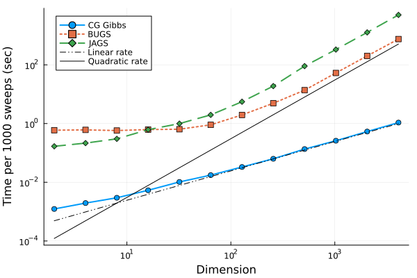
Figure 4: Time taken to perform 1000 sweeps versus dimension for various Gibbs sampler implementations on synthetic logistic regression data sets (lower is better). All samplers considered use a slice sampler within Gibbs.

5.2 Empirical scaling of compute graph Gibbs and NUTS

Next, we empirically compare the time taken to reach a median ESS of 100 as a function of the number of covariates for the Gibbs and Stan NUTS (2.35.0) [8] samplers. To do this, we use the colon cancer data set [1] to create a sequence of logistic regression problems with an increasing number of predictors. Specifically, for each problem we shuffle the order of the covariates and choose an increasing prefix of $d\in\{2^{1},2^{2},\ldots,2^{10},2000\}$ features from the data set (the full data set has 2000 features) to be predictors for the response and use a Gaussian prior with standard deviation 10 for the parameters. To obtain posterior samples, we use CGGibbs and Stan NUTS and compare their effectiveness as the dimension increases. Note that by adding covariates we change not only the dimensionality but also the condition number of the target distribution. The results are shown in Fig. 5. From the figure, we see that the efficiency of CGGibbs scales better in dimension compare to Stan NUTS.

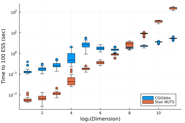
Figure 5: Time taken to achieve an ESS of 100 (median across marginals) for CGGibbs and Stan NUTS as a function of dimension (lower is better). Predictors are added from the colon cancer data set logistic regression model.

Upon closer inspection of Fig. 5, there appears to be a change in behaviour in the performance of CGGibbs when $d\approx n$ (the colon data set has $n=62$ observations). To investigate this, we perform the same experiment but with a varying number of observations with $n\in\{2^{3},2^{4},2^{5}\}$ and record the number of sweeps taken to reach a median ESS of 100. Fig. 6 confirms that there is again a similar transition from when $d<n$ to $d>n$. As shown in Fig. 7, this behaviour is partially explained with the stabilization (or decrease) of various notions of condition number when $d$ increases past $n$. Interestingly, the decrease to sweeps to 100 ESS is similar to a result from Qin and Wang, [36], where they developed a lower bound for the convergence rate of a random scan Gibbs sampler for submodels that depend on the full model.

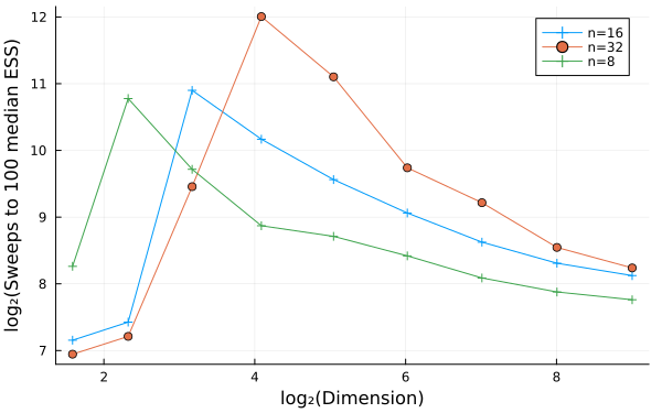
Figure 6: Dimensional scaling of the number of Gibbs sweeps taken to achieve a median ESS of 100 for different data sizes. Samples and predictors are taken from the colon cancer data set.

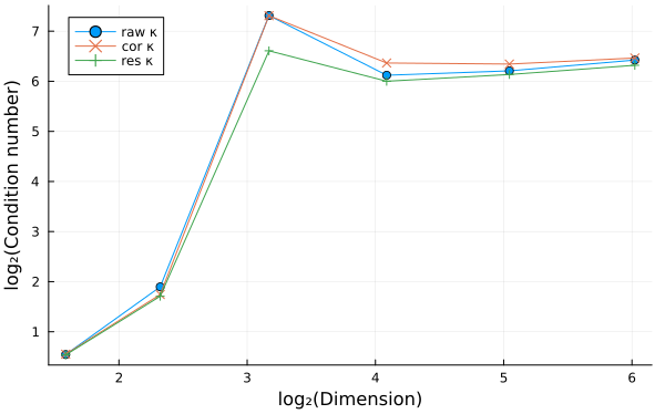
Figure 7: Dimensional scaling of various notions of condition number notions for the logistic regression model with the colon cancer data set. The sample size is set at $n=16$.

5.3 Panel of datasets

We compare the time taken to reach an ESS of 100 (median across all marginals) for CGGibbs and Stan NUTS on 8 binary classification data sets. These data sets include three newsgroup data sets [23], six gene expression data sets [15, 1, 40], and an artificial data set [17]. These data sets vary in size from $n=60$ to $n=2600$ observations, as well as from $d=500$ to $d=7129$ predictors. Across the data sets, $d/n$ ranges from $0.1927$ to $99.0278$. We use a logistic regression model on each data set with Gaussian priors with a standard deviation of 10 for each of the parameters. Each run is repeated with 30 different seeds.

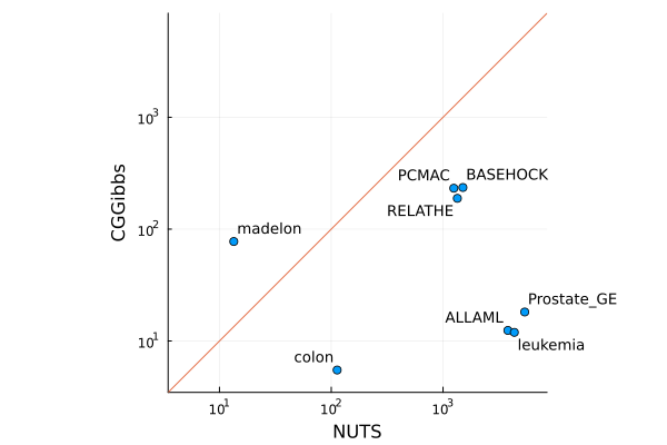
Figure 8: Median time taken to achieve a median ESS of 100 for CGGibbs and Stan NUTS on 8 logistic regression real data sets with a Gaussian prior. Points in the lower triangle indicate that CGGibbs outperformed NUTS.

The outcome of these experiments is summarized in Figs. 8 and 9. These results suggest a correlation between the $d/n$ ratio and the performance of CGGibbs relative to NUTS, which agrees with earlier results from the synthetic experiments.

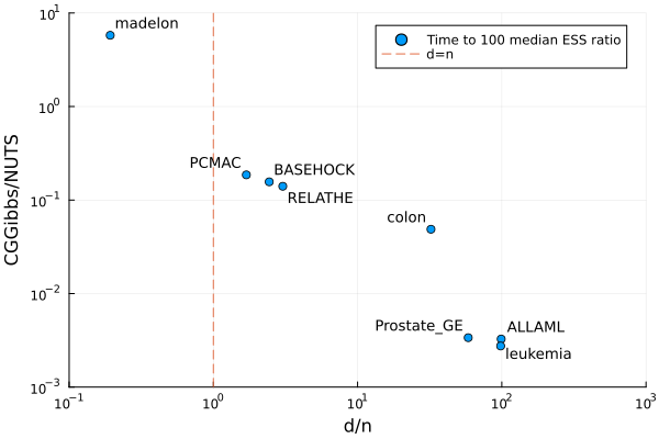
Figure 9: Ratio of median time taken to achieve a median ESS of 100 between CGGibbs and Stan NUTS versus the $d/n$ ratio. Each point represents one of eight logistic regression data sets with a Gaussian prior. The line indicates where $d=n$.

6 Discussion

In this work we demonstrate that the Gibbs sampler is an often overlooked competitor to HMC for a certain class of problems, which includes GLMs. Because of a special structure in the compute graph for the likelihood evaluation after a single-coordinate GLM parameter update on $d$ dimensions, we establish that an $O(d)$ speedup compared to classical implementations of the Gibbs sampler is possible. For GLMs, we show empirically that this speedup often, but not always, leads to our Gibbs implementation outperforming modern implementations of NUTS in terms of dimensional scaling measured by the time it takes to reach a desired effective sample size. An interesting direction for future work is the construction of algorithms combining the strengths of both Gibbs and HMC, such as studying the optimal design of block HMC-within-Gibbs algorithms.

Interestingly, both our CGGibbs algorithm and reverse-mode automatic differentiation, (the key ingredient to automate the use of HMC in PPLs [29]) are based on related but distinct notions of compute graphs. While we have focused on GLMs for concreteness, the efficient update of the compute graph described in Section 3 appears to apply more generally. Automatic processing of arbitrary compute graphs for efficient CGGibbs updates is potentially simpler than the machinery needed for reverse-mode automatic differentiation: in the former case, only certain reduce operations such as addition need special treatment, whereas in the latter case, all primitive operations need to be handled individually (i.e., each provided with a dedicated adjoint). Beyond GLMs, other examples of potential uses of CGGibbs include models with sufficient statistics and models of random or infinite dimensionality.

Acknowledgements

ABC and TC acknowledge the support of an NSERC Discovery Grant. NS acknowledges the support of a Vanier Canada Graduate Scholarship. We additionally acknowledge use of the ARC Sockeye computing platform from the University of British Columbia.

 

Supplementary Materials

 

Appendix A Details of experiments

A.1 CGGibbs algorithm

1:Initial regression parameters $\beta^{(0)}$, prior $\pi_{0}=\otimes_{j=1}^{d}\pi_{0,j}$, observations $\{(x_{i},y_{i})\}_{i=1}^{n}$, inverse link function $\mu$, response distribution $f_{Y|X}$ (mean parametrization), # MCMC iterations $T$, conditional Markov kernel proposals $\{Q_{j|-j}\}_{j=1}^{d}$, conditional targets $\{\pi_{j|-j}\}_{j=1}^{d}$

2:for $i$ in 1, 2, …, $n$ do $\triangleright$ One-time $O(dn)$ cache of linear predictors

3:     $\texttt{cache}[i]\leftarrow\sum_{j=1}^{d}\beta_{j}x_{ij}$

4:end for

5:$\beta\leftarrow\beta^{(0)}$

6:for $t$ in 1, 2, …, $T$ do

7:     for $j$ in 1, 2, …, $d$ do

8:         $\beta_{j}^{\prime}\sim Q_{j|-j}(\cdot|\beta_{-j})$ $\triangleright$ Metropolis-within-Gibbs proposal

9:         $\ell\leftarrow 0$

10:         for $i$ in 1, 2, …, $n$ do $\triangleright$ Increment log-likelihood

11:              $\texttt{linear\_predictor}\leftarrow\texttt{cache}[i]-\beta_{j}x_{ij}+\beta_{j}^{\prime}x_{ij}$

12:              $\ell\leftarrow\ell+\log(f_{Y|X}(y_{i}|\mu(\texttt{linear\_predictor})))$

13:         end for

14:         $U\leftarrow\text{Unif}(0,1)$

15:         $\alpha\leftarrow\texttt{MH\_probability}(\ell,\pi_{j|-j},Q(\cdot|\beta_{-j}),\pi_{0,j})$ $\triangleright$ Acceptance probability

16:         if $U\leq\alpha$ then $\triangleright$ Accept proposal

17:              for $i$ in 1, 2, …, $n$ do $\triangleright$ $O(n)$ update of cache

18:                  $\texttt{cache}[i]\leftarrow\texttt{cache}[i]-\beta_{j}x_{ij}+\beta_{j}^{\prime}x_{ij}$

19:              end for

20:              $\beta_{j}\leftarrow\beta_{j}^{\prime}$ $\triangleright$ Update parameter

21:         end if

22:     end for

23:     $\beta^{(t)}\leftarrow\beta$

24:end for

25:return $\{\beta^{(t)}\}_{t=0}^{T}$

Algorithm 1 Compute graph Gibbs for GLMs ($T$ passes over all parameters)

A.2 Impact of irrelevant parameters on Gibbs mixing rate

To further examine the effect of varying the number features on the Gibbs sampler, as seen in Section 5.2, we generate three synthetic logistic regression data sets where only a prefix of the features influence the outcome. Specifically, each data set has

Design matrix: $$\quad x=(x_{1},x_{2},\ldots,x_{n})^{\top}\in\mathbb{R}^{n\times d},$$ (31)

True parameter: $$\quad\theta=(a,\theta_{s},\textbf{0})\in\mathbb{R}^{d},$$ (32)

Logistic outcome: $$\quad y_{i}|x_{i}\sim{\mathrm{Bern}}(\text{logistic}(a+\theta^{\top}x_{i})),\quad i=1,\ldots,n,$$ (33)

where $d=2^{15},n=20,x_{i}\in\mathbb{R}^{d}$ for all $i=1,\ldots,n$, $a\in\mathbb{R}$ is the intercept and $\theta_{s}\in\mathbb{R}^{30}$ is the coefficient vector for the significant features. The design matrices for each scenario are as follows:

1. Set $x_{i}\sim\mathcal{N}(0,I_{d})$ for all $i=1,\ldots,n$. In this setting, the features are uncorrelated.

2. Set $x_{i}$ the same as scenario (1) for all $i\leq 30$ and set $x_{i}=x_{1}$ for all $i>30$. Here, extra features are perfectly correlated with the first (significant) feature.

3. Set $x_{i}$ the same as scenario (1) for all $i\leq 30$ and set $x_{i}=\textbf{0}$ for all $i>30$.

The results of these experiments are shown in Fig. 10. We show the results for this experiment in terms of the number of sweeps taken to get to a minimum ESS of $100$. The results confirm the surprising findings of Section 5.2 that adding more features can help the Gibbs sampler even if the added features are not related to the data generation process—depending on how “well behaved” the extra features are. In the case of an overparameterized GLM, the irrelevant dimensions might be related to the auxiliary variables used in data augmentation samplers [41]. We suspect that the extra features let the parameters move more freely in a larger state space, thereby speeding up the overall mixing of the chain. It seems that the Gibbs sampler can actually benefit from overparameterization.

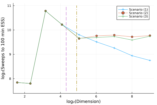
Figure 10: Effect of extra features on the number of Gibbs sweeps taken to achieve a minimum ESS of 100 in different scenarios: (1) no multicollinearity in the design matrix, (2) multicollinearity present in the design matrix, and (3) irrelevant features are identically zero. The dashed line is where $d=n$ and the dash-dotted line is where the “irrelevant features” start to be added.

Appendix B Proofs

In this section we prove Theorem 4.1 and Proposition 4.3.

B.1 Proof of Theorem 4.1

Proof of Theorem 4.1.

To establish the convergence rate of DUGS, we first define some relevant matrices. Let

$$\Sigma=\begin{pmatrix}\Sigma_{11}&\Sigma_{12}&\ldots&\Sigma_{1d}\\ \Sigma_{21}&\Sigma_{22}&\ldots&\Sigma_{2d}\\ \vdots&\vdots&\ddots&\vdots\\ \Sigma_{d1}&\Sigma_{d2}&\ldots&\Sigma_{dd}\end{pmatrix},\qquad\Sigma^{-1}:=Q=\begin{pmatrix}Q_{11}&Q_{12}&\ldots&Q_{1d}\\ Q_{21}&Q_{22}&\ldots&Q_{2d}\\ \vdots&\vdots&\ddots&\vdots\\ Q_{d1}&Q_{d2}&\ldots&Q_{dd}\end{pmatrix}.$$ (34)

Define

$$A(\Sigma)=I-\operatorname{diag}(Q_{11}^{-1},Q_{22}^{-1},\ldots,Q_{dd}^{-1})Q,$$ (35)

and let $L(\Sigma)$ be a block lower triangular matrix such that the lower triangle blocks coincide with those of $A(\Sigma)$. Finally, set $U(\Sigma)=A(\Sigma)-L(\Sigma)$ and define

$$B(\Sigma)=(I-L(\Sigma))^{-1}U(\Sigma).$$ (36)

We express the convergence rate for each metric in terms of the spectral radius of the matrix $B(\Sigma)$, denoted $\rho(B(\Sigma))$, which is the modulus of the eigenvalue of $B(\Sigma)$ with the largest modulus. From Lemma B.1, we have that

$$\rho(B(\Sigma))\leq\exp\left(-\frac{1}{\kappa(\Sigma)}\right).$$ (37)

TV bound.

First, we prove that the rate of convergence of DUGS in TV distance is given by $\rho(B(\Sigma))$. From Theorem 1 of [38], we have $\pi_{t}:=K_{\text{DUGS}}^{t}(x,\cdot)=\mathcal{N}(\mu_{t},\Sigma_{t})$ for all $t\geq 0$, where

$$\mu_{t} =\mu+B(\Sigma)^{t}(\mu_{0}-\mu),\qquad\Sigma_{t}=\Sigma+B(\Sigma)^{t}(\Sigma_{0}-\Sigma)(B(\Sigma)^{\top})^{t}$$ (38)

with $\mathcal{N}(\mu_{0},\Sigma_{0})$ being the initial distribution. (I.e., here $\mu_{0}=x$ and $\Sigma_{0}=0$.) By Pinsker’s inequality, we can bound the total variation with the KL divergence, and the KL divergence between two Gaussians has a closed-form expression, so that

$$\operatorname{TV}(\pi,\pi_{t}) \leq\mathchoice{{\hbox{$\displaystyle\sqrt{\frac{1}{2}\operatorname{KL}(\pi||\pi_{t})\,}$}\lower 0.4pt\hbox{\vrule height=9.66666pt,depth=-7.73337pt}}}{{\hbox{$\textstyle\sqrt{\frac{1}{2}\operatorname{KL}(\pi||\pi_{t})\,}$}\lower 0.4pt\hbox{\vrule height=7.5pt,depth=-6.00003pt}}}{{\hbox{$\scriptstyle\sqrt{\frac{1}{2}\operatorname{KL}(\pi||\pi_{t})\,}$}\lower 0.4pt\hbox{\vrule height=5.25pt,depth=-4.20003pt}}}{{\hbox{$\scriptscriptstyle\sqrt{\frac{1}{2}\operatorname{KL}(\pi||\pi_{t})\,}$}\lower 0.4pt\hbox{\vrule height=4.83331pt,depth=-3.86667pt}}}$$ (39)

$$=\frac{1}{\mathchoice{{\hbox{$\displaystyle\sqrt{2\,}$}\lower 0.4pt\hbox{\vrule height=6.44444pt,depth=-5.15558pt}}}{{\hbox{$\textstyle\sqrt{2\,}$}\lower 0.4pt\hbox{\vrule height=6.44444pt,depth=-5.15558pt}}}{{\hbox{$\scriptstyle\sqrt{2\,}$}\lower 0.4pt\hbox{\vrule height=4.51111pt,depth=-3.6089pt}}}{{\hbox{$\scriptscriptstyle\sqrt{2\,}$}\lower 0.4pt\hbox{\vrule height=3.22221pt,depth=-2.57779pt}}}}\mathchoice{{\hbox{$\displaystyle\sqrt{\operatorname{tr}(\Sigma^{-1}\Sigma_{t}-I)+(\mu-\mu_{t})^{\top}\Sigma^{-1}(\mu-\mu_{t})-\log\det(\Sigma_{t}\Sigma^{-1}).\,}$}\lower 0.4pt\hbox{\vrule height=9.44444pt,depth=-7.55559pt}}}{{\hbox{$\textstyle\sqrt{\operatorname{tr}(\Sigma^{-1}\Sigma_{t}-I)+(\mu-\mu_{t})^{\top}\Sigma^{-1}(\mu-\mu_{t})-\log\det(\Sigma_{t}\Sigma^{-1}).\,}$}\lower 0.4pt\hbox{\vrule height=9.44444pt,depth=-7.55559pt}}}{{\hbox{$\scriptstyle\sqrt{\operatorname{tr}(\Sigma^{-1}\Sigma_{t}-I)+(\mu-\mu_{t})^{\top}\Sigma^{-1}(\mu-\mu_{t})-\log\det(\Sigma_{t}\Sigma^{-1}).\,}$}\lower 0.4pt\hbox{\vrule height=6.63889pt,depth=-5.31114pt}}}{{\hbox{$\scriptscriptstyle\sqrt{\operatorname{tr}(\Sigma^{-1}\Sigma_{t}-I)+(\mu-\mu_{t})^{\top}\Sigma^{-1}(\mu-\mu_{t})-\log\det(\Sigma_{t}\Sigma^{-1}).\,}$}\lower 0.4pt\hbox{\vrule height=5.13889pt,depth=-4.11113pt}}}$$ (40)

We analyze the convergence for each of the terms inside the square root. By Eq. 38,

$$\operatorname{tr}(\Sigma^{-1}\Sigma_{t}-I) =\operatorname{tr}\left(\Sigma^{-1}(\Sigma+B(\Sigma)^{t}(\Sigma_{0}-\Sigma)(B(\Sigma)^{t})^{\top})-I\right)$$ (41)

$$=\operatorname{tr}(\Sigma^{-1}B(\Sigma)^{t}(\Sigma_{0}-\Sigma)(B(\Sigma)^{t})^{\top})$$ (42)

$$=O(\rho(B(\Sigma))^{2t}),$$ (43)

where the asymptotic rate is due to the fact that $B(\Sigma)^{t}$ converges to 0 element-wise at rate $\rho(B(\Sigma))$ [38, Lemma 4]. Similarly, combining Eq. 38 and the convergence of $B(\Sigma)^{t}$, we have that

$$\|\mu-\mu_{t}\|=\|B^{t}(\mu-\mu_{0})\|=O(\rho(B(\Sigma))^{t}),$$ (44)

yielding

$$(\mu-\mu_{t})^{\top}\Sigma^{-1}(\mu-\mu_{t})=O(\rho(B(\Sigma))^{2t}).$$ (45)

For the third term, we obtain that

$$\lvert\log\det(\Sigma_{t}\Sigma^{-1})\rvert =\lvert\log\det(I+B(\Sigma)^{t}(\Sigma_{0}-\Sigma)(B(\Sigma)^{t})^{\top}\Sigma^{-1})\rvert$$ (46)

$$\leq\operatorname{tr}(B(\Sigma)^{t}(\Sigma_{0}-\Sigma)(B(\Sigma)^{t})^{\top}\Sigma^{-1})$$ (47)

$$=O(\rho(B(\Sigma))^{2t}).$$ (48)

Finally, combining Eq. 40 and Eqs. 41, 45 and 46 yields

$$\operatorname{TV}(\pi,\pi_{t})=O(\rho(B(\Sigma))^{t}).$$ (49)

Wasserstein bounds.

Next, we prove the Wasserstein bounds. For two Gaussian distributions $\pi_{1}=\mathcal{N}(\mu_{1},\Sigma_{1})$ and $\pi_{2}=\mathcal{N}(\mu_{2},\Sigma_{2})$, we have the following formula for their Wasserstein 2-distance:

$$\operatorname{W}_{2}^{2}(\pi_{1},\pi_{2})=\|\mu_{1}-\mu_{2}\|_{2}^{2}+\operatorname{tr}(\Sigma_{1}+\Sigma_{2}-2(\Sigma_{2}^{1/2}\Sigma_{1}\Sigma_{2}^{1/2})^{1/2}),$$ (50)

where $\operatorname{tr}(M)$ is the trace of the matrix $M$ and $M^{1/2}$ is the principal square root of $M$. Applying (50) to $\pi_{1}=\pi_{t}=\mathcal{N}(\mu_{t},\Sigma_{t})$ and $\pi_{2}=\pi=\mathcal{N}(\mu,\Sigma)$ gives us

$$\operatorname{W}_{2}^{2}(\pi,\pi_{t}) =\|\mu-\mu_{t}\|_{2}^{2}+\operatorname{tr}(\Sigma+\Sigma_{t}-2(\Sigma^{1/2}\Sigma_{t}\Sigma^{1/2})^{1/2})$$ (51)

$$=\|B(\Sigma)^{t}(\mu_{0}-\mu)\|_{2}^{2}+\operatorname{tr}(2\Sigma+B(\Sigma)^{t}(\Sigma_{0}-\Sigma)(B(\Sigma)^{\top})^{t})$$ (52)

$$\qquad\qquad-2\operatorname{tr}(\Sigma^{1/2}(\Sigma+B(\Sigma)^{t}(\Sigma_{0}-\Sigma)(B(\Sigma)^{\top})^{t})\Sigma^{1/2})^{1/2})$$ (53)

$$=\|B(\Sigma)^{t}(\mu_{0}-\mu)\|_{2}^{2}+2\operatorname{tr}(\Sigma)+\operatorname{tr}(B(\Sigma)^{t}(\Sigma_{0}-\Sigma)(B(\Sigma)^{\top})^{t})$$ (54)

$$\qquad\qquad-2\operatorname{tr}((\Sigma^{2}+(\Sigma^{1/2}B(\Sigma)^{t}(\Sigma_{0}-\Sigma)(B(\Sigma)^{\top})^{t}\Sigma^{1/2})^{1/2})$$ (55)

$$=\|B(\Sigma)^{t}(\mu_{0}-\mu)\|_{2}^{2}+2\operatorname{tr}(\Sigma)+\operatorname{tr}(M_{t})-2\operatorname{tr}((\Sigma^{2}+(\Sigma^{1/2}M_{t}\Sigma^{1/2})^{1/2}),$$ (56)

where $M_{t}:=B(\Sigma)^{t}(\Sigma_{0}-\Sigma)(B(\Sigma)^{\top})^{t}$. We bound the last term in the above expression using the fact

$$\exists\ \epsilon\in(0,1):\ \operatorname{tr}\left(4\frac{1-\epsilon}{\epsilon^{2}}\Sigma-M_{t}\right)\geq 0\quad\forall\ t\geq 0.$$ (57)

This is easy to confirm since the range of the function $g(\epsilon)=4\frac{1-\epsilon}{\epsilon^{2}}$ in $(0,1)$ is $(0,\infty)$ and the matrix in the trace is symmetric. With this, we have

$$\operatorname{tr}\left(4\frac{1-\epsilon}{\epsilon^{2}}\Sigma-M_{t}\right)\geq 0.$$ (58)

$$\Leftrightarrow\ \operatorname{tr}\left(4\frac{1-\epsilon}{\epsilon^{2}}\Sigma M_{t}-M_{t}^{2}\right)\geq 0.$$ (59)

$$\Leftrightarrow\ \operatorname{tr}\left((1-\epsilon)\Sigma M_{t}-\frac{\epsilon^{2}}{4}M_{t}^{2}\right)\geq 0.$$ (60)

$$\Leftrightarrow\ \operatorname{tr}\left(\Sigma M_{t}\right)\geq\operatorname{tr}\left(\epsilon\Sigma M_{t}+\frac{\epsilon^{2}}{4}M_{t}^{2}\right).$$ (61)

$$\Leftrightarrow\ \operatorname{tr}\left(\Sigma^{2}+\Sigma M_{t}\right)\geq\operatorname{tr}\left(\Sigma^{2}+\epsilon\Sigma M_{t}+\frac{\epsilon^{2}}{4}M_{t}^{2}\right).$$ (62)

$$\Leftrightarrow\ \operatorname{tr}\left(\Sigma^{2}+\Sigma^{1/2}M_{t}\Sigma^{1/2}\right)\geq\operatorname{tr}\left(\left(\Sigma+\frac{\epsilon}{2}M_{t}\right)^{2}\right).$$ (63)

Finally, since the square root operation is monotone increasing, we have

$$\operatorname{tr}\left((\Sigma^{2}+\Sigma^{1/2}M_{t}\Sigma^{1/2})^{1/2}\right)\geq\operatorname{tr}(\Sigma)+\frac{\epsilon}{2}\operatorname{tr}(M_{t}).$$ (64)

Plugging (64) into (51) gives us

$$\operatorname{W}_{2}^{2}(\pi,\pi_{t}) \leq\|B(\Sigma)^{t}(\mu_{0}-\mu)\|_{2}^{2}+2\operatorname{tr}(\Sigma)+\operatorname{tr}(M_{t})-2\operatorname{tr}(\Sigma)-\epsilon\operatorname{tr}(M_{t})$$ (65)

$$=\|B(\Sigma)^{t}(\mu_{0}-\mu)\|_{2}^{2}+(1-\epsilon)\operatorname{tr}(M_{t})$$ (66)

$$=\|B(\Sigma)^{t}(\mu_{0}-\mu)\|_{2}^{2}+(1-\epsilon)\operatorname{tr}(B(\Sigma)^{t}(\Sigma_{0}-\Sigma)(B(\Sigma)^{\top})^{t}).$$ (67)

Combining this with Lemma 4 from [38], we have

$$\operatorname{W}_{2}^{2}(\pi,\pi_{t})=O(\rho(B(\Sigma))^{2t})$$ (68)

which shows the convergence rate for Wasserstein 2 distance. By properties of the Wasserstein distance, it follows that $\operatorname{W}_{1}(\pi_{t},\pi)\leq\operatorname{W}_{2}(\pi_{t},\pi)$ and hence $\operatorname{W}_{1}(\pi_{t},\pi)=O(\rho(B(\Sigma))^{t})$.

Chi-squared bound.

For the Pearson-$\chi^{2}$ divergence, the result follows from direct application of Theorem 1 and Lemma 4 of [26]. Namely, we have that

$$\chi^{2}(\pi_{t},\pi)=O(\rho(B(\Sigma))^{t}).$$ (69)

∎

Lemma B.1.

Under the conditions of Theorem 4.1,

$$\rho(B(\Sigma))\leq\exp\left(-\frac{1}{\kappa(\Sigma)}\right).$$ (70)

Proof of Lemma B.1.

Our proof proceeds in two steps, using results from Roberts and Sahu, [38]. We first establish a bound on the $L^{2}$ convergence rate of the random sweep Gibbs sampler (RSGS), $\rho_{L^{2}}(RSGS,\Sigma)$, in terms of $d$ and $\kappa(\Sigma)$. This rate is easier to study as it involves the matrix $A(\Sigma)$ instead of $B(\Sigma)$. We then conclude that $\rho(B(\Sigma))\leq\rho_{L^{2}}(RSGS,\Sigma)$ from an existing result in Roberts and Sahu, [38].

For any symmetric positive definite matrix $\Sigma$, there exists a rotation matrix $R$ that makes $R^{-1}\Sigma R$ diagonal. Furthermore, the condition number $\kappa(\Sigma)$ of the Gaussian distribution with covariance $\Sigma$ is invariant to rotations. Therefore, we can consider $\mathcal{N}(\mu,\Sigma)$ with a fixed condition number, diagonal covariance matrix $\Sigma$ and its rotations without loss of generality. Now, for any matrix $M$, denote $\lambda(M)$ its set of eigenvalues and $D_{M}$ the inverse of the diagonal of $M$ if it has invertible diagonal elements. Let $\lambda_{1}\geq\ldots\lambda_{d}>0$ denote the eigenvalues of $\Sigma$ so that $\kappa(\Sigma)=\lambda_{1}/\lambda_{d}$. Rotating $\mathcal{N}(\mu,\Sigma)$ using a rotation matrix $R$ gives us $\mathcal{N}(R\mu,R\Sigma R^{\top})$. The RSGS coordinate update matrix for $\mathcal{N}(R\mu,R\Sigma R^{\top})$ is

$$A(R\Sigma R^{\top})=I-D_{RQR^{\top}}RQR^{\top}.$$ (71)

To study the maximum eigenvalue of this matrix, we first note two matrix properties. First, for all symmetric positive definite matrices $M,N$, using the spectral norm, we have the inequality

$$\frac{1}{\min\lambda(MN)}=\|(MN)^{-1}\|\leq\|M^{-1}\|\|N^{-1}\|=\frac{1}{\min\lambda(M)}\frac{1}{\min\lambda(N)}.$$ (72)

Also, since $\sum_{j=1}^{d}r^{2}_{i,j}=1$ for the matrix $R$, we have

$$\sum_{j=1}^{d}\frac{r^{2}_{i,j}}{\lambda_{j}}\geq\sum_{j=1}^{d}\frac{r^{2}_{i,j}}{\lambda_{1}}=\frac{1}{\lambda_{1}}.$$ (73)

Combining these results, we have

$$\max\lambda(A(R\Sigma R^{\top})) =1-\min\lambda(D_{RQR^{\top}}RQR^{\top})$$ (74)

$$\leq 1-\min\lambda(D_{RQR^{\top}})\min\lambda(RQR^{\top})$$ (75)

$$=1-\min\lambda(D_{RQR^{\top}})\min\lambda(Q)$$ (76)

$$=1-\min\lambda(D_{RQR^{\top}})\lambda_{d}$$ (77)

$$=1-\lambda_{d}\min_{i}\sum_{j=1}^{d}\frac{r^{2}_{i,j}}{\lambda_{j}}$$ (78)

$$=1-\frac{1}{\kappa(\Sigma)}.$$ (79)

Now, let $\text{rot}_{d}$ be the set of $d$ by $d$ rotation matrices. By Theorem 2 in [38], we have

$$\rho_{L^{2}}(RSGS,\Sigma) \leq\sup_{R\in\text{rot}_{d}}\rho_{L^{2}}(RSGS,R\Sigma R^{\top})$$ (80)

$$=\sup_{R\in\text{rot}_{d}}\left(\frac{1}{d}(d-1+\max\lambda(A(R\Sigma R^{\top})))\right)^{d}$$ (81)

$$\leq\left(\frac{1}{d}\left(d-1+1-\frac{1}{\kappa(\Sigma)}\right)\right)^{d}$$ (82)

$$\leq\exp\left(-\frac{1}{\kappa(\Sigma)}\right).$$ (83)

Finally, combining Eq. 49, Eq. 80 and Theorems 4 and 6 in [38] gives us

$$\rho(B(\Sigma))=\rho_{L^{2}}(DUGS,\Sigma)\leq\rho_{L^{2}}(RSGS,\Sigma)\leq\exp\left(-\frac{1}{\kappa(\Sigma)}\right).$$ (84)

∎

B.2 Proof of Proposition 4.3

Let $\Sigma^{\prime}:=D\Sigma D$ be the covariance matrix after diagonal preconditioning using the diagonal matrix $D$ and set $Q^{\prime}=(\Sigma^{\prime})^{-1}=D^{-1}\Sigma^{-1}D^{-1}$.

$$A(\Sigma^{\prime}) =I-\operatorname{diag}((Q^{\prime})_{11}^{-1},(Q^{\prime})_{22}^{-1},\ldots,(Q^{\prime})_{dd}^{-1})Q^{\prime}$$ (85)

$$=DD^{-1}-D\operatorname{diag}(Q_{11}^{-1},Q_{22}^{-1},\ldots,Q_{dd}^{-1})D^{-1}DQD^{-1}$$ (86)

$$=D(I-\operatorname{diag}(Q_{11}^{-1},Q_{22}^{-1},\ldots,Q_{dd}^{-1})Q)D^{-1}$$ (87)

$$=DA(\Sigma)D^{-1}$$ (88)

$$=D(U(\Sigma)+L(\Sigma))D^{-1}$$ (89)

$$=DU(\Sigma)D^{-1}+DL(\Sigma)D^{-1}.$$ (90)

Since $DU(\Sigma)D^{-1}$ and $DL(\Sigma)D^{-1}$ are upper and lower triangular matrices, respectively, we get

$$U(\Sigma^{\prime})=DU(\Sigma)D^{-1},\quad L(\Sigma^{\prime})=DL(\Sigma)D^{-1}.$$ (91)

Next, we have

$$B(\Sigma^{\prime}) =(I-L(\Sigma^{\prime}))^{-1}U(\Sigma^{\prime})$$ (92)

$$=(DD^{-1}-DL(\Sigma)D^{-1})^{-1}DU(\Sigma)D^{-1}$$ (93)

$$=D(I-L(\Sigma))^{-1}U(\Sigma)D^{-1}$$ (94)

$$=DB(\Sigma)D^{-1}.$$ (95)

Now, let $\lambda$ and $x$ be an eigenvalue and eigenvector of $B(\Sigma^{\prime})$, then

$$B(\Sigma^{\prime})x=\lambda x$$ (96)

$$\Leftrightarrow DB(\Sigma)D^{-1}x=\lambda x$$ (97)

$$\Leftrightarrow B(\Sigma)(D^{-1}x)=D^{-1}\lambda x.$$ (98)

Therefore, $D^{-1}x$ is an eigenvector of $B(\Sigma)$ and $\lambda$ is an eigenvalue of $B(\Sigma)$ so that any eigenvalue of $B(\Sigma^{\prime})$ is an eigenvalue of $B(\Sigma)$. Similarly, we also have any eigenvalue of $B(\Sigma)$ is an eigenvalue of $B(\Sigma^{\prime})$. Hence, $B(\Sigma)$ and $B(\Sigma^{\prime})$ have the same set of eigenvalues which means they also have the same maximum eigenvalue modulus. That is, $\rho(B(\Sigma))=\rho(B(\Sigma^{\prime}))$.

References

- Alon et al., [1999] Alon, U., Barkai, N., Notterman, D. A., Gish, K., Ybarra, S., Mack, D., and Levine, A. J. (1999). Broad patterns of gene expression revealed by clustering analysis of tumor and normal colon tissues probed by oligonucleotide arrays. Proceedings of the National Academy of Sciences, 96(12):6745–6750.
- Andrieu, [2016] Andrieu, C. (2016). On random- and systematic-scan samplers. Biometrika, 103(3):719–726.
- Apers et al., [2022] Apers, S., Gribling, S., and Szilágyi, D. (2022). Hamiltonian Monte Carlo for efficient Gaussian sampling: Long and random steps.
- Ascolani, [2022] Ascolani, F. (2022). Mixing times of a Gibbs sampler for probit hierarchical models. In International Conference on Bayesian Statistics in Action, pages 67–76. Springer.
- Ascolani et al., [2024] Ascolani, F., Roberts, G. O., and Zanella, G. (2024). Scalability of Metropolis-within-Gibbs schemes for high-dimensional Bayesian models. arXiv:2403.09416.
- Ascolani and Zanella, [2024] Ascolani, F. and Zanella, G. (2024). Dimension-free mixing times of Gibbs samplers for Bayesian hierarchical models. The Annals of Statistics, 52(3):869–894.
- Beskos et al., [2013] Beskos, A., Pillai, N. S., Roberts, G. O., Sanz-Serna, J. M., and Stuart, A. M. (2013). Optimal tuning of the hybrid Monte Carlo algorithm. Bernoulli, 19(5A):1501–1534.
- Carpenter et al., [2017] Carpenter, B., Gelman, A., Hoffman, M. D., Lee, D., Goodrich, B., Betancourt, M., Brubaker, M. A., Guo, J., Li, P., and Riddell, A. (2017). Stan: A probabilistic programming language. Journal of statistical software, 76.
- Chen et al., [2020] Chen, Y., Dwivedi, R., Wainwright, M. J., and Yu, B. (2020). Fast mixing of Metropolized Hamiltonian Monte Carlo: Benefits of multi-step gradients. Journal of Machine Learning Research, 21(92):1–72.
- Chen and Gatmiry, [2023] Chen, Y. and Gatmiry, K. (2023). When does Metropolized Hamiltonian Monte Carlo provably outperform Metropolis-adjusted Langevin algorithm? arXiv preprint arXiv:2304.04724.
- Chen and Vempala, [2022] Chen, Z. and Vempala, S. S. (2022). Optimal convergence rate of Hamiltonian Monte Carlo for strongly logconcave distributions. Theory of Computing, 18:1–18.
- Chib and Greenberg, [1995] Chib, S. and Greenberg, E. (1995). Understanding the metropolis-hastings algorithm. The american statistician, 49(4):327–335.
- Gelman et al., [2013] Gelman, A., Carlin, J. B., Stern, H. S., Dunson, D. B., Vehtari, A., and Rubin, D. B. (2013). Bayesian Data Analysis. Chapman and Hall/CRC, 3rd edition edition.
- Geman and Geman, [1984] Geman, S. and Geman, D. (1984). Stochastic relaxation, Gibbs distributions, and the Bayesian restoration of images. IEEE Transactions on Pattern Analysis and Machine Intelligence, 6(6):721–741.
- Golub et al., [1999] Golub, T. R., Slonim, D. K., Tamayo, P., Huard, C., Gaasenbeek, M., Mesirov, J. P., Coller, H., Loh, M. L., Downing, J. R., Caligiuri, M. A., et al. (1999). Molecular classification of cancer: Class discovery and class prediction by gene expression monitoring. Science, 286(5439):531–537.
- Greenwood et al., [1998] Greenwood, P. E., McKeague, I. W., and Wefelmeyer, W. (1998). Information bounds for Gibbs samplers. The Annals of Statistics, 26(6):2128–2156.
- Guyon et al., [2004] Guyon, I., Gunn, S., Ben-Hur, A., and Dror, G. (2004). Result analysis of the NIPS 2003 feature selection challenge. Advances in Neural Information Processing Systems, 17.
- He et al., [2016] He, B. D., De Sa, C. M., Mitliagkas, I., and Ré, C. (2016). Scan order in Gibbs sampling: Models in which it matters and bounds on how much. Advances in Neural Information Processing Systems, 29.
- Hird and Livingstone, [2023] Hird, M. and Livingstone, S. (2023). Quantifying the effectiveness of linear preconditioning in Markov chain Monte Carlo. arXiv:2312.04898.
- Hoffman and Gelman, [2014] Hoffman, M. D. and Gelman, A. (2014). The No-U-Turn Sampler: Adaptively setting path lengths in Hamiltonian Monte Carlo. Journal of Machine Learning Research, 15(47):1593–1623.
- Jiang, [2023] Jiang, Q. (2023). On the dissipation of ideal Hamiltonian Monte Carlo sampler. Stat, 12.
- Jordan, [2004] Jordan, M. I. (2004). Graphical Models. Statistical Science, 19(1):140–155.
- Lang, [1995] Lang, K. (1995). NewsWeeder: Learning to filter netnews. In Machine Learning Proceedings, pages 331–339. Elsevier.
- Langmore et al., [2019] Langmore, I., Dikovsky, M., Geraedts, S., Norgaard, P., and Von Behren, R. (2019). A condition number for Hamiltonian Monte Carlo. arXiv:1905.09813.
- Lee et al., [2020] Lee, Y. T., Shen, R., and Tian, K. (2020). Logsmooth gradient concentration and tighter runtimes for Metropolized Hamiltonian Monte Carlo. In Conference on learning theory, pages 2565–2597. PMLR.
- Li and Geng, [2005] Li, K. and Geng, Z. (2005). Convergence rate of Gibbs sampler and its application. Science in China Series A: Mathematics, 48:1430–1439.
- Livingstone and Zanella, [2022] Livingstone, S. and Zanella, G. (2022). The Barker Proposal: Combining Robustness and Efficiency in Gradient-Based MCMC. Journal of the Royal Statistical Society Series B: Statistical Methodology, 84(2):496–523.
- Lunn et al., [2009] Lunn, D., Spiegelhalter, D., Thomas, A., and Best, N. (2009). The BUGS project: Evolution, critique and future directions. Statistics in Medicine, 28(25):3049–3067.
- Margossian, [2019] Margossian, C. C. (2019). A review of automatic differentiation and its efficient implementation. WIREs Data Mining and Knowledge Discovery, 9(4):e1305.
- Neal, [1996] Neal, R. M. (1996). Bayesian Learning for Neural Networks, volume 118 of Lecture Notes in Statistics. Springer.
- Neal, [2003] Neal, R. M. (2003). Slice sampling. The Annals of Statistics, 31(3):705–767.
- Neal et al., [2011] Neal, R. M. et al. (2011). MCMC using Hamiltonian dynamics. Handbook of Markov Chain Monte Carlo, 2(11):2.
- Papaspiliopoulos et al., [2020] Papaspiliopoulos, O., Roberts, G. O., and Zanella, G. (2020). Scalable inference for crossed random effects models. Biometrika, 107(1):25–40.
- Plummer et al., [2003] Plummer, M. et al. (2003). JAGS: A program for analysis of Bayesian graphical models using Gibbs sampling. In Proceedings of the 3rd international workshop on Distributed Statistical Computing, pages 1–10.
- Qin and Jones, [2022] Qin, Q. and Jones, G. L. (2022). Convergence rates of two-component MCMC samplers. Bernoulli, 28(2):859–885.
- Qin and Wang, [2024] Qin, Q. and Wang, G. (2024). Spectral telescope: Convergence rate bounds for random-scan Gibbs samplers based on a hierarchical structure. The Annals of Applied Probability, 34(1B):1319–1349.
- Roberts and Rosenthal, [2015] Roberts, G. O. and Rosenthal, J. S. (2015). Surprising convergence properties of some simple gibbs samplers under various scans. International Journal of Statistics and Probability, 5(1):51–60.
- Roberts and Sahu, [1997] Roberts, G. O. and Sahu, S. K. (1997). Updating schemes, correlation structure, blocking and parameterization for the Gibbs sampler. Journal of the Royal Statistical Society Series B: Statistical Methodology, 59(2):291–317.
- Román et al., [2014] Román, J. C., Hobert, J. P., and Presnell, B. (2014). On reparametrization and the Gibbs sampler. Statistics & Probability Letters, 91:110–116.
- Singh et al., [2002] Singh, D., Febbo, P. G., Ross, K., Jackson, D. G., Manola, J., Ladd, C., Tamayo, P., Renshaw, A. A., D’Amico, A. V., Richie, J. P., et al. (2002). Gene expression correlates of clinical prostate cancer behavior. Cancer Cell, 1(2):203–209.
- Tanner and Wong, [1987] Tanner, M. A. and Wong, W. H. (1987). The calculation of posterior distributions by data augmentation. Journal of the American Statistical Association, 82(398):528–540.
- Wang and Wibisono, [2023] Wang, J.-K. and Wibisono, A. (2023). Accelerating Hamiltonian Monte Carlo via Chebyshev integration time. In International Conference on Learning Representations.
- Wang, [2017] Wang, N.-Y. (2017). Convergence rates of the random scan Gibbs sampler under the Dobrushin’s uniqueness condition. Electronic Communications in Probability, 22:1–7.
- Wang, [2019] Wang, N.-Y. (2019). Convergence rates of symmetric scan Gibbs sampler. Frontiers of Mathematics in China, 14:941–955.
- Wang and Wu, [2014] Wang, N.-Y. and Wu, L. (2014). Convergence rate and concentration inequalities for Gibbs sampling in high dimension. Bernoulli, 20(4):1698–1716.
- Wang and Yin, [2020] Wang, N.-Y. and Yin, G. (2020). Convergence rates of the blocked Gibbs sampler with random scan in the Wasserstein metric. Stochastics, 92(2):265–274.
- Zanella and Roberts, [2021] Zanella, G. and Roberts, G. (2021). Multilevel linear models, Gibbs samplers and multigrid decompositions (with discussion). Bayesian Analysis, 16(4):1309–1391.