Universal adapters between quantum LDPC codes

Abstract

We propose the repetition code adapter as a way to perform joint logical Pauli measurements within a quantum low-density parity check (LDPC) codeblock or between separate such codeblocks. This adapter is universal in the sense that it works regardless of the LDPC codes involved and the Paulis being measured. The construction achieves joint logical Pauli measurement of $t$ weight $O(d)$ operators using $O(td\log^{2}d)$ additional qubits and checks and $O(d)$ time. We also show for some geometrically-local codes in fixed $D\geq 2$ dimensions that only $O(td)$ additional qubits and checks are required instead. By extending the adapter in the case $t=2$, we construct a toric code adapter that uses $O(d^{2})$ additional qubits and checks to perform targeted logical CNOT gates on arbitrary LDPC codes via Dehn twists. To obtain some of these results, we develop a novel weaker form of graph edge expansion.

1 Introduction

The long-term promise of quantum computing and quantum algorithms will undoubtedly rely on the backbone of quantum error correction (QEC) and fault tolerance. While early experiments focused on demonstrating the building blocks of QEC [1, 2, 3, 4, 5], recently there has been increased focus on scaling up the distance [6] and encoding rate of QEC codes [7]. This is coupled with a line of theoretical research towards increasing QEC code parameters [8, 9, 10, 11, 12, 13], culminating with the recent establishment of good quantum low-density parity check (LDPC) codes [14, 15, 16]. These theoretical models are of experimental interest as LDPC codes are constructed, by design, to limit the connectivity between qubits with the hope of simplifying experimental requirements of the physical systems that will eventually realize these codes.

Although much of the progress has centered on improving the encoding rate and distance of LDPC codes, the relative number of encoded logical qubits along with the ability to protect errors, of equal importance is establishing a model for doing logical computation in these codes. The earliest techniques for addressing logical computation centered around methods developed for gate teleportation [17], where special ancilla states are prepared offline [18, 19, 20, 21], yet the space-time overhead for reliably preparing these states can be punitive as the code size increases, and other techniques have been more recently explored in the theoretical literature. One of the leading approaches is that of lattice surgery in the surface code [22], where an additional surface code patch can be prepared and fused to the original code, allowing for the joint-measurement of their respective logical operators. Given the success of this approach to the surface code [23] which itself is an LDPC code, it was natural to ask if a similar type of approach could be adapted for more general LDPC codes. Inspired by ideas originally motivated towards weight reduction of quantum codes [24, 25, 26], this line of research led to recent schemes for quantum LDPC surgery [27, 28, 29, 30, 31, 32].

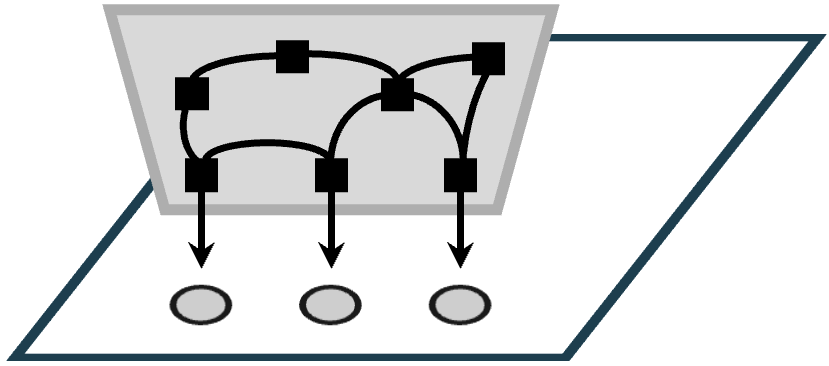
(a) Gauging measurement

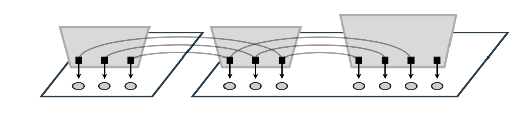
(b) Repetition code adapters for joint logical measurement

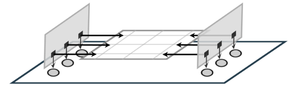
(c) Toric code adapter for logical gates

Figure 1: (a) For an arbitrary LDPC code (drawn as a rectangular patch), gauging measurement [31] of a logical Pauli operator works by attaching a stabilizer state defined on an appropriate auxiliary graph (gray area) to the qubit support of the logical operator (gray circles) creating a deformed code in which the logical operator becomes a stabilizer. Only some graph vertices, which represent checks, connect 1-to-1 to the logical support. This set of vertices is referred to as a port. In this work, we construct additional tools: (b) The ports of several auxiliary graphs can be connected together with carefully chosen adapters (curved edges) while keeping the deformed code LDPC. This measures the product of logical Pauli operators without measuring any individually. Adapters can connect operators in the same codeblock or separate blocks and regardless of their structure. Mathematically, our adapter construction relies on a sparse basis transformation for the classical repetition code, which we call the $\mathsf{SkipTree}$ algorithm. (c) Similarly, an arbitrary LDPC code can be merged with a toric code (or other codes) to perform logical gates.

In this work, we build upon the gauging measurement framework of Ref. [31], which we briefly summarize now. The goal is to measure an arbitrary logical Pauli operator on an arbitrary LDPC code. The main idea is to find an appropriate auxiliary graph $\mathcal{G}$, where ancilla qubits reside on edges and stabilizer checks are associated to both vertices and cycles. This auxiliary graph is merged with the original code by forcing a subset of the vertex checks to interact with the qubits in the support of the logical operator being measured, see Fig 1(a). As a result, the stabilizers of the original code are deformed and care must be taken to avoid deforming into a non-LDPC code or suffering a deformed code with reduced code distance. Doing so necessitates several nontrivial properties of the auxiliary graph $\mathcal{G}$, including the existence of certain short perfect matchings, the existence of a suitably sparse cycle basis, and edge expansion.

Our main result addresses a practical problem in the gauging measurement construction. Because computing with quantum LDPC surgery naturally lends itself to Pauli-based computation [33] (analogously to surface code lattice surgery [23]), one naively expects the need to measure potentially any logical Pauli operator and thus that exponentially many auxiliary graphs with suitable properties will need to be constructed. This task can be greatly simplified if suitably constructed auxiliary graphs to measure individual logical operators, say those on single logical qubits, could simply be connected in some way to measure the product of those operators instead while maintaining the necessary graph properties. For logical operators with isomorphic auxiliary subgraphs, this connection can be done directly [30], but it is a priori unclear how to do these joint measurements more generally.

Here, we solve this joint measurement problem in very general setting. Our solution is universal in the sense that it works regardless of the structure of the codes or logical operators involved, provided only the operators act on disjoint sets of qubits. We are able to adapt the structure of any auxiliary graph to any other, connecting them via a set of adapter edges into one large graph, see Fig. 1(b). This builds on the idea of a bridge system from Ref. [29], but with new tools to guarantee the resulting deformed code for the product measurement is LDPC and suffers no loss of code distance. Moreover, these adapters can be further modified to couple to other ancillary systems with other desirable properties. Namely, we present a method to merge an arbitrary LDPC code with the toric code along the supports of two disjoint logical operators, Fig. 1(c). From there, a unitary circuit suffices to implement a logical $\mathsf{CNOT}$ using a method inspired by the Dehn twist $\mathsf{CNOT}$ from Refs. [34, 35, 36]. This is an explicit example of how adapters can be used as a tool for mapping between codes with different properties, such as those with large rate for space-efficient memory and those with additional symmetries enabling fault-tolerant logical computation.

The auxiliary graphs and adapters necessitate additional qubits and thus increase the space overhead for fault-tolerant computation. Gauging measurement of a single operator of weight $d$ uses $O(d\log^{2}d)$ additional qubits in general, and connecting these systems with our adapters to measure the product of $t$ such operators takes $O(td\log^{2}d)$ additional qubits. The $\log^{2}d$ factor exists to ensure that the auxiliary graph has a suitably sparse cycle basis through use of the decongestion lemma [37]. However, we also show that for geometrically-local LDPC codes we can use the Delaunay triangulation [38] of the set of points representing a logical operators to construct an auxiliary graph that does not require decongestion, thereby improving the overhead of gauging measurement in this special case. In contrast, regardless of this decongestion result, the toric code adapter is asymptotically inefficient in that it uses $O(d^{2})$ additional qubits, but has three potential advantages at finite size: (1) it does not require edge expansion in the auxiliary graphs that interface between the original code and toric code, (2) these interface systems are alone smaller than existing interfaces between LDPC and surface codes [39], $O(d\log^{2}d)$ qubits compared with $O(d^{2})$, and (3) it directly performs a logical $\mathsf{CNOT}$ gate rather than building the gate through logical measurements. Gauging measurement and our adapter variants all use $O(d)$ time to sufficiently deal with measurement errors.

In Section 2 we review the basics of stabilizer codes and their representation as Tanner graphs. We also review gauging measurement [31] and LDPC surgery concepts from Ref. [29], but through the lens of a novel definition of relative expansion which unifies and simplifies some ideas from these prior works. In Sec. 3, we present an efficient classical algorithm for transforming between different check bases for the classical repetition code, which will be of use in creating our adapters. In Sec. 4, we present the repetition code adapter for measuring joint logical operators in general LDPC codes that works be connecting individual graphs with relative expansion into one large graph guaranteed to have relative expansion. Sec. 5 provides a method for appending an adapter that allows for the application of a unitary targeted logical $\mathsf{CNOT}$ gate and avoids the requirement of relative expansion. In Sec. 6, we give a method for constructing appending graphs for geometrically-local codes that are naturally LDPC and avoid the need for additional overhead due to decongestion.

2 Preliminaries

2.1 Stabilizer codes and Tanner graphs

An $n$-qubit hermitian Pauli operator can be written $i^{u\cdot v}X(u)Z(v)$, where $u,v\in\mathbb{F}_{2}^{n}$, or simply as a symplectic vector $[u|v]$. Vectors in this paper are always by default row vectors and must be transposed, e.g. $v^{\top}$, to obtain a column vector. If $v=0$ (resp. $u=0$), we say the Pauli is $X$-type (resp. $Z$-type). Several Pauli operators written in symplectic notation can be gathered together as the rows of a symplectic check matrix

$$H=[H_{X}|H_{Z}]\in\mathbb{F}_{2}^{\;r\times 2n},\;\text{such that}\;H\left(\begin{array}[]{cc}0&I\\ I&0\end{array}\right)H^{\top}=0,$$ (1)

where we use $I$ to denote the identity matrix of context-dependent size (here $n$), and the condition guarantees that all Pauli operators in the set commute with one another. Thus, $H$ describes the checks of a stabilizer code [40].

Logical operators of a stabilizer code are Pauli operators that commute with all the checks. All the checks are logical operators also. Logical operators that are not a product of checks are called nontrivial. The code distance is the minimum Pauli weight of any nontrivial logical operator.

We can illustrate a stabilizer code by drawing a Tanner graph. This is a bipartite graph containing a vertex for each qubit and each check (a row of $H$). A qubit is connected to each check in which it participates with an edge labeled $[1|0]$, $[0|1]$, or $[1|1]$ depending on whether the check acts on the qubit as $X$, $Z$, or $Y$.

However, in cases with where multiple qubits and checks share identical check matrices, drawing a Tanner graph with a single node for every individual qubit and check requires too much specific detail. We abstract away the detail by drawing Tanner graphs with qubits gathered into named sets, say $\mathcal{Q}_{0}$, $\mathcal{Q}_{1}$, $\mathcal{Q}_{2}$,…, and checks gathered into named sets, say $\mathcal{C}_{0}$, $\mathcal{C}_{1}$, $\mathcal{C}_{2}$, …. An edge is drawn between $\mathcal{C}_{i}$ and $\mathcal{Q}_{j}$ if any check from $\mathcal{C}_{i}$ acts on any qubit in $\mathcal{Q}_{j}$. Label the edge with a symplectic matrix $[C_{X}|C_{Z}]\in\mathbb{F}_{2}^{|\mathcal{Q}_{i}|\times 2|\mathcal{C}_{j}|}$ indicating which checks act on which qubits and with what type of Pauli operator. For instance, the entire stabilizer code from Eq. (1) is drawn as in Fig. 2a.

(a)

(b)

(c)

Figure 2: Example Tanner graphs with qubit sets drawn as circles and check sets drawn as squares. (a) A generic stabilizer code, (b) a CSS code, and (c) the distance $d$ toric code. In the toric code, each set of qubits and checks contains $d$ objects.

For CSS codes [41, 42], there is a basis of checks in which each check is either $X$-type or $Z$-type. In the Tanner graph of such a code, if a set of checks $\mathcal{C}_{i}$ is entirely $X$-type, instead of labeling each edge with a symplectic matrix like $[C_{X}|0]$, we simply label the check set with $X$ and each edge with $C_{X}$ only. We handle sets of $Z$-type checks analogously. The Tanner graph of a CSS code is shown in Fig. 2b.

We can alternatively view sets $\mathcal{C}_{i}$ and $\mathcal{Q}_{j}$ as vector spaces instead and abuse notation to denote both the sets and the vector spaces with these symbols. For example, a vector $v\in\mathbb{F}_{2}^{|\mathcal{C}_{i}|}$ indicates a subset of checks from $\mathcal{C}_{i}$ by its nonzero elements. We write $\mathcal{H}(v\in\mathcal{C}_{i})$ to denote the product of this subset of checks, i.e. it is an $n$-qubit Pauli operator. If all checks in the set are $X$-type or $Z$-type, we write $\mathcal{H}_{X}(v\in\mathcal{C}_{i})$ or $\mathcal{H}_{Z}(v\in\mathcal{C}_{i})$ instead. Likewise, a Pauli operator on qubit set $\mathcal{Q}_{j}$ is denoted by $X(u_{x}\in\mathcal{Q}_{j})Z(u_{z}\in\mathcal{Q}_{j})$ for appropriate vectors $u_{x},u_{z}\in\mathbb{F}_{2}^{|\mathcal{Q}_{j}|}$.

We can perform calculations in this notation with matrix-vector multiplication over $\mathbb{F}_{2}$. For instance, if the check set $\mathcal{C}_{i}$ is connected to only a single qubit set $\mathcal{Q}_{j}$ with edge labeled $[C_{X}|C_{Z}]$, then

$$\mathcal{H}(v\in\mathcal{C}_{i})=X(vC_{X}\in\mathcal{Q}_{j})Z(vC_{Z}\in\mathcal{Q}_{j}).$$ (2)

If a family of stabilizer codes with growing code size $n$ is $(\alpha,\beta)$ low-density parity-check (LDPC), it has a basis of checks in which each check acts on at most $\alpha=O(1)$ qubits and each qubit is acted upon by at most $\beta=O(1)$ checks. This translates to the sparsity of the code’s parity check matrix $H=[H_{X}|H_{Z}]$. We say a matrix over $\mathbb{F}_{2}$ is $(r,c)$-sparse if the maximum row weight is at most $r$ and the maximum column weight is at most $c$. If both $H_{X}$ and $H_{Z}$ are $(r,c)$-sparse then the code is $(2r,2c)$ LDPC.

One outstanding family of quantum LDPC codes is the toric code family [43], depicted as a Tanner graph in Fig. 2c. There, we use $H_{C}$ to denote the canonical cyclic parity check matrix of the classical repetition code, i.e.

$$H_{C}=\left(\begin{array}[]{ccccc}1&1&&\dots&\\ &1&1&&\\ &\vdots&&\ddots&\\ 1&&&&1\end{array}\right).$$ (3)

Denote by $e_{i}$ the length-$n$ vector with a 1 in only the $i\;(\text{mod}\;n)$ position. We can define a cyclic shift matrix $C\in\mathbb{F}_{2}^{\;n\times n}$ that acts as $e_{i}C=e_{i+1}$ for all $i$. Then, $H_{C}=I+C$. The only vector in the nullspace of $H_{C}$ is the vector of all 1s, denoted $\vec{1}$, so $\vec{1}H_{C}=H_{C}\vec{1}^{\;\top}=0$. In general, we let the sizes of $e_{i}$, $\vec{1}$, $I$, $C$, and $H_{C}$ be context dependent.

2.2 Graphs and expansion

We write $\mathcal{G}=(\mathcal{V},\mathcal{E})$ to signify a graph with vertex set $\mathcal{V}$ of size $n$ and an edge set $\mathcal{E}$ of size $m$. An alternative description is provided by the incidence matrix $G=\mathbb{F}_{2}^{\;m\times n}$, a matrix in which each row represents an edge, each column represents a vertex, and $G_{ij}=1$ if and only if edge $i$ contains vertex $j$. If the maximum vertex degree of $\mathcal{G}$ is $w$, then $G$ is $(2,w)$-sparse.

If $\mathcal{G}$ has $p$ connected components, a complete cycle basis can be specified by a matrix $N$ over $\mathbb{F}_{2}$ satisfying $NG=0$ and $\mathrm{rank}(N)=m-n+p$, known as the cyclomatic number of the graph (e.g. see [44, 45]). We say the cycle basis is $(r,c)$-sparse if $N$ is an $(r,c)$-sparse matrix. In an $(r,c)$-sparse cycle basis, each basis cycle is no longer than $r$ edges and each edge is in no more than $c$ basis cycles.

We characterize the edge expansion of a graph via its Cheeger constant. Intuitively, this is a measure of how bottlenecked a graph is – if a graph contains a large set of vertices with very few outgoing edges, the Cheeger constant of that graph is small. We also define a novel relative version of edge expansion.

Definition 1.

Let $\mathcal{G}=(\mathcal{V},\mathcal{E})$ be a graph on $n=|\mathcal{V}|$ vertices and $m=|\mathcal{E}|$ edges. Let $G\in\mathbb{F}_{2}^{\;m\times n}$ be the incidence matrix of this graph. The expansion (also known as the Cheeger constant or isoperimetric number [46]) $\beta(\mathcal{G})$ of this graph is the largest real number such that, for all $v\in\mathbb{F}_{2}^{n}$ (i.e. all subsets of vertices),

$$|vG^{\top}|\geq\beta(\mathcal{G})\min(|v|,n-|v|).$$ (4)

More generally, the expansion relative to a vertex subset $\mathcal{U}\subseteq\mathcal{V}$ and parameterized by integer $t>0$, denoted $\beta_{t}(\mathcal{G},\mathcal{U})$, is the largest real number such that, for all $v\in\mathbb{F}_{2}^{n}$,

$$|vG^{\top}|\geq\beta_{t}(\mathcal{G},\mathcal{U})\min(t,|u|,|\mathcal{U}|-|u|),$$ (5)

where we use $u$ to denote the restriction of $v$ to vertices $\mathcal{U}$. Note that $\beta(\mathcal{G})=\beta_{|\mathcal{V}|}(\mathcal{G},\mathcal{V})$. We sometimes refer to $\beta(\mathcal{G})$ as the global expansion to distinguish it from the relative expansion.

Any graph always has relative expansion at least as large as its global expansion, i.e. $\beta_{t}(\mathcal{G},\mathcal{U})\geq\beta(\mathcal{G})$ for all $\mathcal{U}\subseteq\mathcal{V}$ and $t>0$. This is important for our purposes because we will develop some techniques to guarantee a graph has sufficient relative expansion (to ensure a good quantum code distance) but not necessarily large global expansion. The relation between expansions is a corollary of the following simple lemma.

Lemma 2.

Suppose $\mathcal{G}=(\mathcal{V},\mathcal{E})$ is a graph and $\mathcal{U},\mathcal{U}^{\prime}\subseteq\mathcal{V}$ are subsets of vertices. If $\mathcal{U}^{\prime}\subseteq\mathcal{U}$ and $0<t^{\prime}\leq t$, then $\beta_{t^{\prime}}(\mathcal{G},\mathcal{U}^{\prime})\geq\beta_{t}(\mathcal{G},\mathcal{U})$.

Proof.

Consider any $u\in\mathbb{F}_{2}^{|\mathcal{U}|}$, and let $u^{\prime}$ be the restriction of $u$ to $\mathcal{U}^{\prime}\subseteq\mathcal{U}$. It follows $|u^{\prime}|\leq|u|$, $|\mathcal{U}^{\prime}|-|u^{\prime}|\leq|\mathcal{U}|-|u|$, and $\min(t,|u^{\prime}|,|\mathcal{U}^{\prime}|-|u^{\prime}|)\leq\min(t,|u|,|\mathcal{U}|-|u|)$. Also, because $t^{\prime}\leq t$,

$$\min(t^{\prime},|u^{\prime}|,|\mathcal{U}^{\prime}|-|u^{\prime}|)\leq\min(t,|u^{\prime}|,|\mathcal{U}^{\prime}|-|u^{\prime}|)\leq\min(t,|u|,|\mathcal{U}|-|u|).$$ (6)

The result now follows by applying the definition of relative expansion. ∎

The relative expansion can diverge significantly from the global expansion. We later show (Lemma 5) that the relative expansion of a graph can be increased to at least 1 by taking a Cartesian graph product with a path graph, while the global expansion cannot be increased this way.

2.3 Gauging measurement

Gauging measurement [31] is a flexible recipe for measuring a logical operator of a quantum code. Because several of our results are best viewed in the context of gauging measurement, we give a review of it here. A novelty of our presentation is the use of relative expansion, which was only implicit in previous works [31, 29].

Suppose $\mathcal{L}$ is the set of qubits supporting the logical operator $\overline{Z}$ to be measured. Here we assume $\overline{Z}$ is a $Z$-type Pauli operator, which is without loss of generality if we choose the appropriate local basis for each qubit of $\mathcal{L}$ and allow the code to be non-CSS.

Figure 3: The deformed code created during gauging measurement of logical operator $\overline{Z}$ supported on qubits $\mathcal{L}$. Edge qubits $\mathcal{E}$ are introduced and vertex checks $\mathcal{V}=\{A_{v}\}_{v}$ and cycle checks $\mathcal{U}=\{B_{c}\}_{c}$ are measured. Here $G$ is the incidence matrix of the graph defining these checks, $N$ is a cycle basis satisfying $NG=0$, and $M$ is a matching matrix that represents support gained by some of the original stabilizers $\mathcal{S}$, specifically, those that have $X$-type support on $\mathcal{L}$. The matrix $F$ has elements $F_{qv}$ for all $q\in\mathcal{L}$ and $v\in\mathcal{V}$ and $F_{qv}=1$ if and only if $f(q)=v$. The rest of the qubits and checks of the original code are drawn on the left but their Tanner graph connectivity does not change during the code deformation.

Introduce an “auxiliary” graph $\mathcal{G}=(\mathcal{V},\mathcal{E})$ and an injective map $f:\mathcal{L}\rightarrow\mathcal{V}$. The function indicates a subset of vertices $\mathrm{im}f=f(\mathcal{L})$, the “port”, at which we attach the original code and the graph. We use $\mathcal{G}$ and $f$ to define a deformed code. Each edge $e$ of this graph is associated to a single qubit with $X(e)$ and $Z(e)$ Pauli operators, each vertex $v$ is associated to a $Z$ check

$$A_{v}=\bigg{\{}\begin{array}[]{ll}Z(q)\prod_{e\ni v}Z(e),&\exists q\in\mathcal{L},f(q)=v\\ \prod_{e\ni v}Z(e),&\mathrm{otherwise}\end{array}$$ (7)

and each cycle $c\subseteq\mathcal{E}$ is associated to an $X$ check

$$B_{c}=\prod_{e\in c}X(e).$$ (8)

If we initialize all edge qubits in $\ket{+}$ and measure all checks $A_{v}$, $B_{c}$, certain checks of the original code must pick up $X$-type support on the edge qubits to commute with all $A_{v}$. These deformed checks are exactly the checks of the original code with $X$-type support (either acting as Pauli $X$ or $Y$) on qubits in $\mathcal{L}$. Suppose such a check $S$ has $X$-type support on qubits $\mathcal{L}_{S}\subseteq\mathcal{L}$. Then after measurement of $A_{v}$, it becomes

$$S\rightarrow S\prod_{e\in\mu(\mathcal{L}_{S})}X(e),$$ (9)

where $\mu(\mathcal{L}_{S})\subseteq\mathcal{E}$ is a perfect matching in $\mathcal{G}$ of vertices $f(\mathcal{L}_{S})$, which exists because $\mathcal{G}$ is connected and $|\mathcal{L}_{S}|$ is even (because $S$ commutes with $\overline{Z}$). All these components of gauging measurement are depicted as a Tanner graph in Fig. 3.

There are additional properties of the auxiliary graph $\mathcal{G}$ and the port function $f:\mathcal{L}\rightarrow\mathcal{V}$ that ensure that gauging measurement results in a suitable deformed code.

Theorem 3 (Graph Desiderata).

[31]

To ensure the deformed code has exactly one less logical qubit than the original code and measures the target logical operator $\overline{Z}=Z(\mathcal{L})$, it is sufficient that

1. $\mathcal{G}$ is connected.

To ensure the deformed code is LDPC, it is necessary and sufficient that

1. $\mathcal{G}$ has $O(1)$ vertex degree.

2. For all stabilizers $S$ of the original code, (a) $|\mu(\mathcal{L}_{S})|=O(1)$, i.e. each stabilizer has a short perfect matching in $\mathcal{G}$, and (b) each edge is in $O(1)$ matchings $\mu(\mathcal{L}_{S})$.

3. There is a cycle basis of $\mathcal{G}$ in which (a) each cycle is length $O(1)$ and (b) each edge is in $O(1)$ cycles.

To ensure the deformed code has code distance at least the distance $d$ of the original code, it is sufficient that

1. $\mathcal{G}$ has relative Cheeger constant $\beta_{d}(\mathcal{G},f(\mathcal{L}))\geq 1$.

Proof.

That desiderata $1,2,3$ are necessary and sufficient for guaranteeing the deformed code is LDPC is evident from the construction. For completeness, we prove the sufficiency of desiderata 0 and 4 for their respective purposes in Appendix A. It is worth noting that a stronger form of desideratum 4 is assumed to prove the deformed code distance in prior work [31], namely that $\beta(\mathcal{G})\geq 1$. Lemma 2 implies this is sufficient for a graph to satisfy our desideratum 4 but is not necessary. ∎

We remark that it is easy to create a graph satisfying desiderata 0, 1 and 2 provided that the original code is LDPC and the operator $\overline{Z}$ to be measured is irreducible, i.e. has no other $Z$-type logical operators supported entirely within it. This can be done by pairing up the vertices in $f(\mathcal{L}_{S})$ for all $S$ and drawing edges between paired vertices. Desiderata 2 is satisfied by construction. The resulting graph must also be connected because the original checks $S$ restricted to qubits in $\mathcal{L}$ must generate the repetition code whenever $\overline{Z}$ is irreducible (see Lemma 9 in Ref. [29]). In addition, the resulting graph is $O(1)$ degree because only $O(1)$ sets $\mathcal{L}_{S}$ can contain any given qubit for an LDPC code. Thus, provided $\overline{Z}$ is irreducible, this recipe leaves only desiderata 3 and 4 to be satisfied. Dealing with the reducible case is one of the main results of this paper, so we leave it until Section 4.

Remarkably, it turns out that provided a graph $\mathcal{G}_{0}$ that satisfies 0, 1 and 2, it can be modified to satisfy all the desiderata simultaneously. This process is illustrated in Fig. 4. The first step is to thicken the graph.

Definition 4 (Thickening).

Suppose $\mathcal{G}_{0}=(\mathcal{V}_{0},\mathcal{E}_{0})$ and $\mathcal{G}_{1}=(\mathcal{V}_{1},\mathcal{E}_{1})$ are two graphs. The Cartesian product [47, 48] is another graph $\mathcal{G}=\mathcal{G}_{0}\square\mathcal{G}_{1}=(\mathcal{V}_{0}\times\mathcal{V}_{1},\mathcal{E})$ where $((u_{0},u_{1}),(v_{0},v_{1}))\in\mathcal{E}$ if and only if either (1) $u_{0}=v_{0}$ and $(u_{1},v_{1})\in\mathcal{E}_{1}$, or (2) $u_{1}=v_{1}$ and $(u_{0},v_{0})\in\mathcal{E}_{0}$.

Let $\mathcal{P}_{L}$ be the path graph with $L$ vertices. Then, we say the graph $\mathcal{G}_{0}^{(L)}=\mathcal{G}_{0}\square\mathcal{P}_{L}$ is $\mathcal{G}_{0}$ thickened $L$ times.

Intuitively, the thickened graph $\mathcal{G}_{0}^{(L)}$ is $L$ copies of $\mathcal{G}_{0}$ stacked on top of one another and connected “transversally”, i.e. each vertex is connected to its copy above and below in the stack (or connected to just one copy of itself if it is at the bottom or top of the stack). See Fig. 4b.

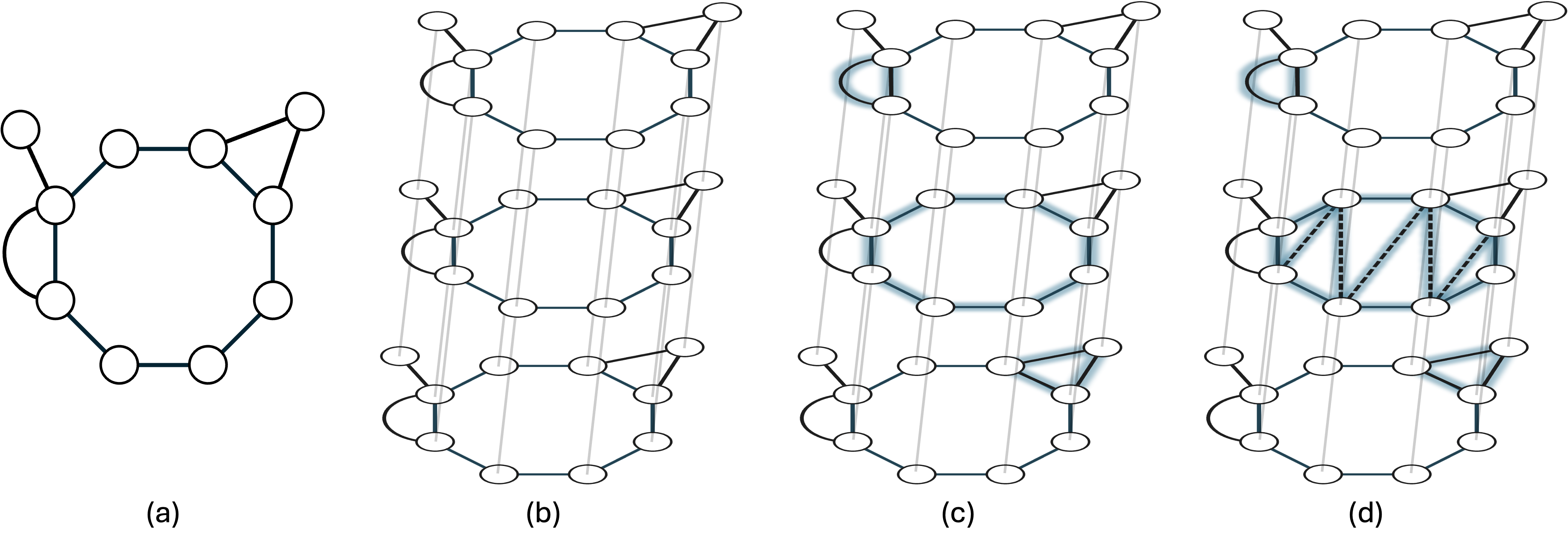
Figure 4: A example of the steps going into constructing a graph $\mathcal{G}$ satisfying all the desiderata of Theorem 3 starting from a graph $\mathcal{G}_{0}$ satisfying just desiderata 0, 1, and 2. (a) The graph $\mathcal{G}_{0}$. (b) The thickened graph $\mathcal{G}^{(L)}_{0}$, here with $L=3$. Note the edges (drawn lighter gray) connecting the corresponding vertices in adjacent layers. (c) A cycle basis for $\mathcal{G}^{(L)}_{0}$ includes every length four cycle constructed from edge $e=(i,j)$ in layer $l$, the copy of edge $e$ in adjacent layer $l+1$, and the lighter gray edges connecting the copies of $i$ and $j$. The cycle basis of $\mathcal{G}^{(L)}_{0}$ also includes (highlighted) one cycle for each cycle in a basis of $\mathcal{G}_{0}$, and each such cycle can be put into any one of the layers independently. A highlighted cycle is equivalent to its copies in other layers by adding to it the length four cycles between layers. (d) Long cycles in the basis can now be cellulated by adding edges (dashed) and including the resulting triangles in the cycle basis instead.

As observed in Ref. [29] (without the relative expansion concept), thickening a graph can increase its relative expansion.

Lemma 5 (Relative Expansion Lemma).

For any connected graph $\mathcal{G}_{0}$, the $L\geq 1/\beta(\mathcal{G}_{0})$ times thickened graph $\mathcal{G}_{0}^{(L)}$ has relative Cheeger constant $\beta_{t}(\mathcal{G}_{0}^{(L)},\mathcal{U})\geq 1$ for any $t>0$ provided $\mathcal{U}\subseteq\mathcal{V}_{0}\times\{l\}$ for some $l=0,1,\dots,L-1$. (i.e. $\mathcal{U}$ is a subset of vertices in any one copy of graph $\mathcal{G}_{0}$).

Proof.

This follows the proof of Lemma 5 in Ref. [29] but suitably generalized to relative expansion. Let $G\in\mathbb{F}_{2}^{m\times n}$ be the incidence matrix of $\mathcal{G}_{0}$ and $G_{L}=\mathbb{F}_{2}^{m_{L}\times n_{L}}$ be the incidence matrix of the thickened graph $\mathcal{G}^{(L)}$. Explicitly, $m_{L}=mL+n(L-1)$, $n_{L}=nL$, and

$$G_{L}=\left(\begin{array}[]{c}I_{L}\otimes G\\ H_{R}\otimes I_{n}\end{array}\right),$$ (10)

where $H_{R}$ is the $L-1\times L$ check matrix of the repetition code, i.e. $H_{C}$ missing its last row.

Let $v_{j}\in\mathbb{F}_{2}^{n}$ for $j=0,1,\dots,L-1$ be vectors indicating choices of vertices from each copy of $\mathcal{G}_{0}$. Also define $v^{\prime}=\mathrm{argmin}_{v_{j}}\min(|v_{j}|,n-|v_{j}|)$. Making judicious use of the triangle inequality and the assumption that $L\beta(\mathcal{G}_{0})\geq 1$, we calculate

$$|(v_{0}\text{ }v_{1}\dots v_{L-1})G_{L}^{\top}| =\sum_{j=1}^{L-1}|v_{j-1}+v_{j}|+\sum_{j=0}^{L-1}|v_{j}G^{\top}|$$ (11)

$$\geq|v^{\prime}+v_{l}|+L\beta(\mathcal{G}_{0})\min(|v^{\prime}|,n-|v^{\prime}|)$$ (12)

$$\geq|v^{\prime}+v_{l}|+\min(|v^{\prime}|,n-|v^{\prime}|)$$ (13)

$$\geq\min(|v_{l}|,n-|v_{l}|).$$ (14)

Let $u\in\mathbb{F}_{2}^{|\mathcal{U}|}$ be the restriction of $v_{l}$ to $\mathcal{U}$. Then $|v_{l}|\geq|u|$ and $n-|v_{l}|\geq|\mathcal{U}|-|u|$, so $|(v_{0}\;v_{1}\dots v_{L-1})G_{L}^{\top}|\geq\min(|u|,|\mathcal{U}|-|u|)\geq\min(t,|u|,|\mathcal{U}|-|u|)$ for all choices of vectors $v_{j}$ and all $t>0$, implying $\beta_{t}(\mathcal{G}_{0}^{(L)},\mathcal{U})\geq 1$. ∎

Because of the Relative Expansion Lemma, we can satisfy Theorem 3, part 4 by sufficiently thickening any initial graph $\mathcal{G}_{0}=(\mathcal{V}_{0},\mathcal{E}_{0})$ and choosing a port function $f:\mathcal{L}\rightarrow\mathcal{V}_{0}\times\{0,1,\dots,L-1\}$ to be injective on $\mathcal{V}_{0}\times\{l\}$ for any $l=0,1,\dots,L-1$.

Thickening also has another use in satisfying the graph desiderata. To see this, we quote (parts of) the decongestion lemma from Freedman and Hastings.

Lemma 6 (Decongestion Lemma).

[37] If $\mathcal{G}=(\mathcal{V},\mathcal{E})$ is a graph with vertex degree $O(1)$, then there exists a cycle basis in which each edge appears in at most $O(\log^{2}|\mathcal{V}|)$ cycles of the basis. Moreover, this basis can be constructed by an efficient randomized algorithm.

As a corollary, for any graph $\mathcal{G}_{0}=(\mathcal{V}_{0},\mathcal{E}_{0})$, the $L=\Omega(\log^{2}|\mathcal{V}_{0}|)$ times thickened graph $\mathcal{G}_{0}^{(L)}$ has a cycle basis in which each edge appears in at most $O(1)$ cycles. The existence of this basis is explained in Fig. 4c.

The combination of Lemmas 5 and 6 implies that, for any graph $\mathcal{G}_{0}$, the $L$ times thickened graph $\mathcal{G}^{(L)}_{0}$ always satisfies desiderata 3b and 4 from Theorem 3, provided $L$ is both $\Omega(\beta(\mathcal{G}_{0})^{-1})$ and $\Omega(\log^{2}|\mathcal{V}|)$. Moreover, if $\mathcal{G}_{0}$ satisfies 1 and 2, then so will $\mathcal{G}^{(L)}_{0}$.

The final step is to satisfy desiderata 3b. This necessitates that $\mathcal{G}^{(L)}_{0}$ not have any cycles that are too long in its cycle basis. However, this can be done by adding enough edges to cellulate large cycles into triangles, Fig. 4d. Because the graph already satisfies 3a, this cellulation cannot increase the degree of any vertex by more than $O(1)$. Moreover, it can only increase the relative expansion. Thus, the cellulated version of $\mathcal{G}^{(L)}_{0}$ is our final graph $\mathcal{G}$. This final graph and the port function $f:\mathcal{L}\rightarrow\mathcal{V}_{0}\times\{l\}$ described above satisfy all desiderata in Theorem 3.

Finally, we note that gauging measurement can be performed with phenomenological fault distance [49] equal to the code distance $d$ of the original code. The phenomenological fault distance is the minimum number of qubit or measurement errors that can cause an undetected logical error (note, other noise in the circuits for measuring checks is not included). We refer to [31] for the proof, but just remark here that this is done by initializing all edge qubits $\mathcal{E}$ in the $\ket{+}$ state, repeating the measurement of the deformed code’s checks at least $d$ times, and finally measuring out all the edge qubits in the $X$ basis. See also similar fault distance proofs for the logical measurement scheme in Ref. [29].

3 The $\mathsf{SkipTree}$ basis transformation

Consider a classical code defined on a connected graph $\mathcal{G}=(\mathcal{V},\mathcal{E})$ with vertices representing $n=|\mathcal{V}|$ bits and edges representing $m=|\mathcal{E}|$ parity checks. It is clear the code is equivalent to a repetition code of length $n$ with an unconventional basis of parity checks. Indeed, the incidence matrix $G\in\mathbb{F}_{2}^{m\times n}$ of the graph is the parity check matrix of the code.

In this section, we ask if we can instead always use a canonical basis of repetition code checks $H_{C}$ such that each of these canonical checks is a product of a constant number (independent of $n$) of the old checks of $G$. We allow bits in the canonical basis to have different indices than they had in the old basis. Thus, our question is equivalent to asking whether there is always a sparse transformation matrix $T\in\mathbb{F}_{2}^{n\times m}$ and permutation $P$ (representing the aforementioned bit relabeling) such that $TGP=H_{C}$.

Our main result is the following.

Theorem 7.

For any connected graph with $n$ vertices and $m$ edges with $m\times n$ incidence matrix $G$, there exists an $n\times m$ $(3,2)$-sparse matrix $T$ and $n\times n$ permutation matrix $P$ such that $TGP=H_{C}$. There is also an algorithm to find $T$ and $P$ that takes $O(n+m)$ time (returning $T$ and $P$ as sparse matrices).

Proof.

We analyze Algorithm 1 that returns $T,P$ given $G$. We assume $n>1$, $m>0$ in the following since otherwise the theorem is trivial. Notably, the number of edges need not be bounded and our algorithm works for high-degree graphs.

The algorithm works by first finding a spanning tree $S$ of the graph $G$. We may choose an arbitrary node $r$ to be the root of $S$, which also uniquely defines parent/child relationships for the whole tree. Finding a spanning tree can be done in $O(n+m)$ time [50] and can be stored in a data structure in which it is constant time to find the children or parent of a given node, e.g. by having each node store the indices of its neighbors in the tree.

Now we proceed recursively with two functions $\mathsf{LabelFirst}$ and $\mathsf{LabelLast}$, both of which take a node in the tree as an argument. In words, $\mathsf{LabelFirst}(i)$ will first label node $i$ with the next unused integer from $\mathbb{Z}_{n}=\{0,1,\dots,n-1\}$ (the next unused integer is tracked globally), and then call $\mathsf{LabelLast}(j)$ on each child $j$ of $i$. Similarly, $\mathsf{LabelLast}(i)$ will call $\mathsf{LabelFirst}(j)$ on each child $j$ of $i$ and, only after all those function calls have finished, will label node $i$ with the next unused integer. Each node is either the argument of a $\mathsf{LabelFirst}$ call or a $\mathsf{LabelLast}$ call (not both), and so is labeled exactly once. Moreover, the “first” and “last” type nodes make a two-coloring of the vertices of the spanning tree (though not necessarily a two-coloring of graph $G$) in the sense that no two first-type nodes are adjacent and no two last-type nodes are adjacent in the spanning tree. First-type nodes are labeled before every other node in their sub-tree, while last-type nodes are labeled after every other node in their sub-tree.

This recursion structure means that very often (though not always), nodes labeled $i$ and $i+1(\mathrm{mod}\text{ }n)$ are not adjacent in the spanning tree but instead have one or two nodes separating them, thus explaining $\mathsf{SkipTree}$ as the algorithm’s name. See Fig. 5 for an example. This is the desired behavior, because (as we show later) we want to make sure that, for all nodes $i$, the shortest path from $i$ to $i+1(\mathrm{mod}\text{ }n)$ in the tree is constant length. Intuitively, this involves traveling up and down the tree, labeling nodes as we go, but when traveling away from the root we should leave some nodes unlabeled so they can be labeled later on the way back to the root.

Although it can be arbitrary, there is an order in which functions $\mathsf{LabelFirst}$ and $\mathsf{LabelLast}$ are called on the children of a node $i$. If $j$ is the first child on which the function is called, we call $j$ the oldest child of $i$. If $j$ is the last on which the function is called, we call $j$ the youngest child of $i$. We introduce the “oldest” and “youngest” terminology to avoid using the words “first” and “last” again. We can also use terms like “next oldest” and “next youngest” to refer to this order of children.

We construct $T$ so that row $i$ picks out the edges of $G$ in the unique shortest path between the node labeled $i$ and the node labeled $i+1(\mathrm{mod}\text{ }n)$ in the spanning tree. Note that only edges in the spanning tree are used in these paths. This is perhaps less than optimal for some graphs but is sufficient to achieve a $T$ of constant sparsity without worrying about the graph structure beyond the spanning tree. We refer to the shortest path between $i$ and $i+1(\mathrm{mod}\text{ }n)$ as path $i$.

Each edge $e=(f,l)$ of the spanning tree is adjacent to a first-type node $f$ and a last-type node $l$, and the label of the last-type node must be larger than the label of the first-type node. If $f$ is the parent of $l$, then path $f$ and path $l$ include the edge $e$. If instead $l$ is the parent of $f$, then path $f-1(\mathrm{mod}\text{ }n)$ and path $l-1(\mathrm{mod}\text{ }n)$ include the edge $e$. In either case, once the edge is used the second time, the entire sub-tree below and including the edge has been labeled, so the edge is not included in any other paths. This shows the column weight of $T$ is exactly two (for all columns corresponding to edges in the spanning tree).

The weight of the $i^{\text{th}}$ row of $T$ is the number of edges in path $i$. We claim the longest a path can be is length three. We show this to complete the proof. An example including all cases encountered in this part of the proof is provided in Fig. 5.

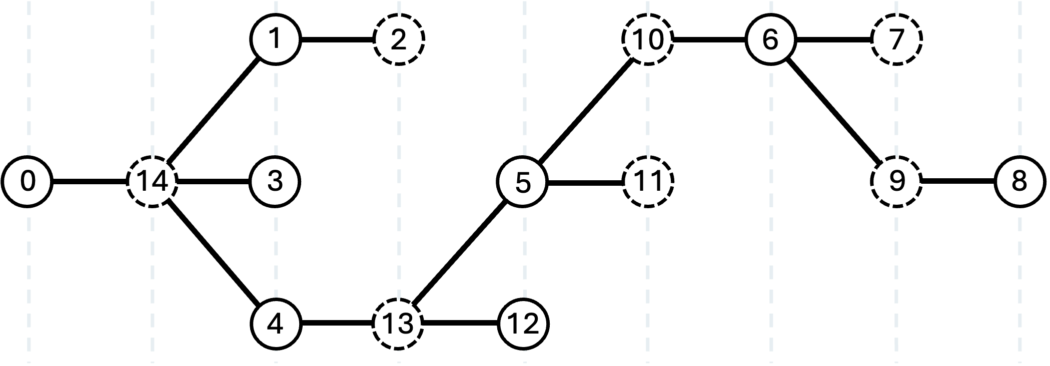
Figure 5: An example spanning tree with nodes labeled according to the $\mathsf{SkipTree}$ algorithm, Algorithm 1. The root node is labeled $0$ on the far left, and first-type nodes are represented with solid circles, while last-type nodes are dashed. Path $i$ is the unique shortest path in the spanning tree from node labeled $i$ to the node labeled $i+1(\mathrm{mod}\text{ }15)$. The proof of Theorem 7 involves arguing that all such paths are length three or less. Examples of all cases encountered in that proof are included in this figure – path 12 for case (1), path 3 for case (2), path 0 for case (3), path 6 for case (4), path 14 for case (a), path 13 for case (b), path 11 for case (c), path 10 for case (d), and path 7 for case (e).

Consider path $i$ where $i$ is a first-type node. Note that the node labeled $n-1$ is always last-type and so $i\neq n-1$. We first assume node $i$ has no children, which also implies $i$ is not the root and it has a parent. There are two sub-cases – (1) if node $i$ is the youngest child of its parent, then its parent will be labeled $i+1$, in which case the path length is one, (2) if node $i$ is not the youngest child of its parent, then its next youngest sibling is labeled $i+1$, in which case the path length is two. Next, assume node $i$ has at least one child. There are again two sub-cases – (3) if the oldest child of $i$ has a child, then node $i+1$ will be a grandchild of $i$, in which case the path length is two, (4) if the oldest child of $i$ does not have a child, then node $i+1$ will be the oldest child of $i$, in which case the path length is one.

Now consider path $i$ where $i$ is a last-type node. Because node $i$ has been labeled, its entire sub-tree has already been labeled with integers $<i$. Also, node $i$ always has a parent because the only parentless node, the root, is first-type. We first assume node $i$ is the youngest child of its parent $p$. There are three sub-cases – (a) Node $p$ has no parent and so is the root, which implies $i=n-1$, $i+1(\mathrm{mod}\text{ }n)=0$, and the path length is one, (b) Node $p$ is the youngest child of its parent, which implies $i+1$ is the grandparent of $i$ and the path length is two, (c) Node $p$ is not the youngest child of its parent, which implies the next youngest child of the parent of $p$ is $i+1$ (i.e. an “uncle” of node $i$) and the path length is three. Now, assume node $i$ is not the youngest child of its parent $p$. There is a next youngest child $y$ and it is a last-type node. There are two sub-cases – (d) $y$ has no children, which implies $y$ is labeled $i+1$ and a path length of two, (e) $y$ has a child, which implies its oldest child is labeled $i+1$ (i.e. a “nephew” of $i$) and the path length is three. ∎

Algorithm 1 Given a connected graph $G\in\mathbb{F}_{2}^{\;m\times n}$, find $T\in\mathbb{F}_{2}^{\;n\times m}$ and permutation matrix $P\in\mathbb{F}_{2}^{\;n\times n}$ such that $TGP=H_{C}$. Both $T$ and $P$ have just $O(n)$ nonzero entries and could be constructed and returned as sparse matrices.

1:$\triangleright$ Note we say “vertex $v$” if it corresponds to the $v^{\text{th}}$ column of $G$. One goal of this algorithm is to label vertices uniquely with integers from $\mathbb{Z}_{n}$ in such a way to guarantee $T$ is sparse. We say “vertex $v$ is labeled $l$” if it acquires label $l\in\mathbb{Z}_{n}$. Of course, $v$ need not equal $l$.

2:procedure $\mathsf{SkipTree}$($G$)

3:     $S\leftarrow$ a spanning tree of $G$ $\triangleright$ has incidence matrix $S_{I}\in\mathbb{F}_{2}^{\;n-1\times n}$ that we do not need to store

4:     Index $\leftarrow 0$

5:     $\mathrm{Label}\leftarrow$ empty list of length $n$

6:     procedure $\mathsf{LabelFirst}$($v$)

7:         $\mathrm{Label}[\mathrm{Index}]\leftarrow v$

8:         Index $\leftarrow$ Index + 1

9:         for each child of vertex $v$ in $S$ do

10:              $\mathsf{LabelLast}(\mathrm{child})$               

11:     procedure $\mathsf{LabelLast}$($v$)

12:         for each child of vertex $v$ in $S$ do

13:              $\mathsf{LabelFirst}(\mathrm{child})$          

14:         $\mathrm{Label}[\mathrm{Index}]\leftarrow v$

15:         Index $\leftarrow$ Index + 1      

16:     $\mathsf{LabelFirst}(0)$ $\triangleright$ we choose the root to be 0. After this line, $\mathrm{Label}[l]=v$ means vertex $v$ is labeled $l$.

17:     $P\leftarrow n\times n$ matrix with $P_{vl}=1$ iff $\mathrm{Label}[l]=v$.

18:     $\tilde{T}\leftarrow$ matrix with $n$ rows and $n-1$ columns.

19:     $\tilde{T}_{le}=1$ iff edge $e$ is part of the shortest path in $S$ from $\mathrm{Label}[l]$ to $\mathrm{Label}[l+1]$. $\triangleright$ now $\tilde{T}S_{I}=H_{C}P^{\top}$

20:     Add zero columns to $\tilde{T}$, obtaining $T$ so that $TG=\tilde{T}S_{I}$.

21:     Return $T$, $P$.

We remark on modifications to the $\mathsf{SkipTree}$ algorithm and special cases. First, we observe that the $\mathsf{SkipTree}$ algorithm can also be used to find $T^{\prime},P^{\prime}$ such that $T^{\prime}GP^{\prime}=H_{R}$ where $H_{R}\in\mathbb{F}_{2}^{(n-1)\times n}$ is the canonical full-rank parity check matrix of the repetition code. That is, $H_{R}$ is $H_{C}$ with the last row removed. Thus, it is clear the $\mathsf{SkipTree}$ algorithm also solves this problem by just removing the last row of $T$ to get $T^{\prime}$ and setting $P^{\prime}=P$. However, we also present a slightly modified version of the $\mathsf{SkipTree}$ algorithm in Appendix C to improve the sparsity of $T^{\prime}$ for some graphs.

If there exists a Hamiltonian cycle in $G$, i.e. a cycle that visits every vertex and uses every edge at most once, then the $\mathsf{SkipTree}$ algorithm is not necessary to solve $TGP=H_{C}$. Instead, $T$ can be chosen to be the $(1,1)$-sparse matrix that selects just those edges from $G$ that are in the Hamiltonian cycle. Likewise, $T^{\prime}GP^{\prime}=H_{R}$ can be solved easily if there exists a Hamiltonian path in $G$. Unfortunately, it is well-known that finding a Hamiltonian cycle or path (or even determining the existence of one) are NP-complete problems.

To conclude this section, we provide some intuition for why Theorem 7 is useful in qLDPC code deformations. Consider some CSS (for simplicity, not necessity) qLDPC code with check matrices $H_{X},H_{Z}$ and a logical $Z$-type operator $L$ of that code. Let $S_{X}$ be the sub-matrix of $H_{X}$ that is supported on $\overline{Z}$. It is known that when $L$ is irreducible (i.e. there is no other $Z$-type logical or stabilizer supported entirely within the support of $\overline{Z}$), then $S_{X}$ is a parity check matrix of a repetition code (see Lemma 9 of [29] or Appendix B). While $S_{X}$ is perhaps not the incidence matrix of a graph (because its rows may have weight larger than two), we can use ideas from gauging measurement [31] to decompose each such higher weight row into a sum of weight two rows, and thus obtain a graph $G$ that is also a parity check matrix for the repetition code. It is this parity check matrix that can undergo a basis change into the repetition code.

For instance, see the Tanner graph in Fig. 6, in which we claim (1) all the checks commute, (2) the code is LDPC, and (3) $Z(\mathcal{L})$ and $Z(\mathcal{Q})$ are equivalent logical operators. The idea encapsulated by this example is the same used to connect codes with repetition code and toric code adapters in Sections 4 and 5. For the adapter constructions, we delve deeper into the details of the deformed codes.

Figure 6: An LDPC code deformation which makes use of Theorem 7 to ensure the code pictured is LDPC and its checks commute. Building on top of the construction in Fig. 3 (left of the dashed line), we introduce edges $T$ and $P$, which are outputs of the $\mathsf{SkipTree}$ algorithm, that connect to new qubits $\mathcal{Q}$ and checks $\mathcal{C}$ having repetition code structure.

4 Repetition code adapter for joint logical measurements

Of practical concern in fault-tolerant quantum computing is the connection of bespoke systems designed to measure two operators $\overline{Z}_{l}$ and $\overline{Z}_{r}$ into one system to measure the product $\overline{Z}_{l}\overline{Z}_{r}$ without measuring either operator individually. The operators $\overline{Z}_{l}$ and $\overline{Z}_{r}$ may be in different codeblocks or the same codeblock. We do require they are non-overlapping so that we can assume they can all be made $Z$-type simultaneously via single-qubit Cliffords. If there are multiple codeblocks, we still refer to them together as the original code, which just happens to be separable.

Figure 7: Measuring $\overline{Z}_{l}\overline{Z}_{r}$ without measuring either logical operator individually. The adapter edges joining auxiliary graphs $G_{l}$ and $G_{r}$ into one larger auxiliary graph are those hosting the qubits $\mathcal{Q}$. The matrices $T_{l},T_{r},P_{l},P_{r}$ are determined using the $\mathsf{SkipTree}$ algorithm, Theorem 7. Differing from Figs. 3 and 6, we do not include in this diagram qubits or checks outside the supports of the logicals $\overline{Z}_{l}$ and $\overline{Z}_{r}$, and instead just suggest their existence through dangling edges. This is left ambiguous because we allow $\overline{Z}_{l}$ and $\overline{Z}_{r}$ to be contained in different codeblocks or the same codeblock. In the latter case, it also may happen that the check sets $\mathcal{S}_{l}$ and $\mathcal{S}_{r}$ share checks, which then gain support on both auxiliary graphs during deformation.

In this section, we solve this joint measurement problem while guaranteeing that the resulting connected graph satisfies all the desiderata of Theorem 3, provided the individual graphs did. A Tanner graph illustration of our construction is shown in Fig. 7. The connection between the individual graphs is done via a bridge of edges, as originally proposed in Ref. [29]. Here, we instead call that set of edges an adapter.

Definition 8.

Provided two graphs $\mathcal{G}_{l}=(\mathcal{V}_{l},\mathcal{E}_{l})$ and $\mathcal{G}_{r}=(\mathcal{V}_{r},\mathcal{E}_{r})$ and vertex subsets $\mathcal{V}_{l}^{*}\subseteq\mathcal{V}_{l}$ and $\mathcal{V}_{r}^{*}\subseteq\mathcal{V}_{r}$ of equal size, an adapter is a set of edges $\mathcal{A}\subseteq\mathcal{V}_{l}^{*}\times\mathcal{V}_{r}^{*}$ defined by a bijective function $a:\mathcal{V}_{l}^{*}\rightarrow\mathcal{V}_{r}^{*}$ so that $(v_{l},v_{r})\in\mathcal{A}$ if and only if $a(v_{l})=v_{r}$. We call the resulting graph $\mathcal{G}=\mathcal{G}_{l}\sim_{\mathcal{A}}\mathcal{G}_{r}=(\mathcal{V}_{l}\cup\mathcal{V}_{r},\mathcal{E}_{l}\cup\mathcal{E}_{r}\cup\mathcal{A})$ the adapted graph.

Given two graphs with sufficient relative expansion on ports $\mathcal{P}_{l}$ and $\mathcal{P}_{r}$, it is relatively straightforward to join them with an adapter between subsets of the ports.

Lemma 9.

If $\mathcal{G}_{l}=(\mathcal{V}_{l},\mathcal{E}_{l})$ has relative expansion $\beta_{t_{l}}(\mathcal{G}_{l},\mathcal{P}_{l})\geq 1$ and $\mathcal{G}_{r}=(\mathcal{V}_{r},\mathcal{E}_{r})$ has relative expansion $\beta_{t_{r}}(\mathcal{G}_{r},\mathcal{P}_{r})\geq 1$, then connecting them with an adapter $\mathcal{A}$ on any subsets $\mathcal{P}_{l}^{*}\subseteq\mathcal{P}_{l}$ and $\mathcal{P}_{r}^{*}\subseteq\mathcal{P}_{r}$ results in an adapted graph $\mathcal{G}=\mathcal{G}_{l}\sim_{\mathcal{A}}\mathcal{G}_{r}$ with relative expansion $\beta_{t}(\mathcal{G},\mathcal{P}_{l}\cup\mathcal{P}_{r})\geq 1$ for $t=\min(t_{l},t_{r},|\mathcal{A}|)$.

Proof.

Note that Ref. [29] contains a similar proof arguing for the code distance of their bridged systems. Here, we have abstracted out the relative expansion idea.

Let $G_{l}$ and $G_{r}$ be the incidence matrices of the graphs $\mathcal{G}_{l}$ and $\mathcal{G}_{r}$, respectively. We write the incidence matrix of $\mathcal{G}$ as

$$G\; =\;\bordermatrix{&\mathcal{V}_{l}&\mathcal{V}_{r}\cr\mathcal{E}_{l}&G_{l}&0\cr\mathcal{A}&A_{l}&A_{r}\cr\mathcal{E}_{r}&0&G_{r}\cr}\qquad$$ (15)

where we have labeled rows and columns by the sets of edges and vertices they represent. Here, the matrix $A_{l}$ has exactly one 1 per row and one 1 in each column corresponding to $\mathcal{P}_{l}^{*}\subseteq\mathcal{V}_{l}$. Restricted to only those columns, $A_{l}$ is a permutation matrix $\pi_{l}$. The same structure holds for matrix $A_{r}$ and $\mathcal{P}_{r}^{*}\subseteq\mathcal{V}_{r}$ with a permutation matrix $\pi_{r}$.

We let $v=(v_{l}\;v_{r})\in\mathbb{F}_{2}^{|\mathcal{V}_{l}|+|\mathcal{V}_{r}|}$ be a vector indicating an arbitrary subset of vertices with $v_{l}$ and $v_{r}$ its restriction to the left and right vertices, respectively. Likewise, $u_{l}$ and $u_{r}$ represent $v$ restricted to $\mathcal{P}_{l}$ and $\mathcal{P}_{r}$ and $u^{*}_{l}$ and $u^{*}_{r}$ its restriction to $\mathcal{P}_{l}^{*}$ and $\mathcal{P}_{r}^{*}$.

Making use of expansion,

$$|vG^{\top}| =|v_{l}G_{l}^{\top}|+|v_{r}G_{r}^{\top}|+|A_{l}v_{l}^{\top}+A_{r}v_{r}^{\top}|$$

$$\geq\min(t_{l},|u_{l}|,|\mathcal{P}_{l}|-|u_{l}|)+\min(t_{r},|u_{r}|,|\mathcal{P}_{r}|-|u_{r}|)+|A_{l}v_{l}^{\top}+A_{r}v_{r}^{\top}|.$$ (16)

Next, we notice that

$$|A_{l}v_{l}^{\top}+A_{r}v_{r}^{\top}|=|\pi_{l}u_{l}^{*\top}+\pi_{r}u_{r}^{*\top}|\geq\max(|u^{*}_{l}|-|u^{*}_{r}|,|u^{*}_{r}|-|u^{*}_{l}|)$$ (17)

using the triangle inequality.

We now consider the different cases that result from evaluating the $\mathrm{min}$ functions in Eq. (16).

1. For vectors $v$ in which the first $\mathrm{min}$ function evaluates $t_{l}$ or the second evaluates to $t_{r}$, we have $|vG^{\top}|\geq\min(t_{l},t_{r})$.

2. If $|u_{l}|\leq|\mathcal{P}_{l}|/2$ and $|u_{r}|\leq|\mathcal{P}_{r}|/2$, we have $|vG^{\top}|\geq|u_{l}|+|u_{r}|\geq|u_{lr}|$ where by $u_{lr}$ we mean the restriction of $v$ to $\mathcal{P}_{l}\cup\mathcal{P}_{r}$.

3. If $|u_{l}|\geq|\mathcal{P}_{l}|/2$ and $|u_{r}|\geq|\mathcal{P}_{r}|/2$, we have $|vG^{\top}|\geq|\mathcal{P}_{l}|-|u_{l}|+|\mathcal{P}_{r}|-|u_{r}|\geq|\mathcal{P}_{l}\cup\mathcal{P}_{r}|-|u_{lr}|$.

4. If $|u_{l}|\leq|\mathcal{P}_{l}|/2$ and $|u_{r}|\geq|\mathcal{P}_{r}|/2$, then

   $$|vG^{\top}| \geq|u_{l}|+|\mathcal{P}_{r}|-|u_{r}|+\max(|u^{*}_{l}|-|u^{*}_{r}|,|u^{*}_{r}|-|u^{*}_{l}|)$$ (18)

   $$\geq|\mathcal{P}_{r}|+(|u_{l}|-|u_{l}^{*}|)-(|u_{r}|-|u_{r}^{*}|)$$ (19)

   $$\geq|\mathcal{P}_{r}|-(|u_{r}|-|u_{r}^{*}|)$$ (20)

   $$\geq|\mathcal{P}_{r}^{*}|=|\mathcal{A}|.$$ (21)

5. If $|u_{l}|\geq|\mathcal{P}_{l}|/2$ and $|u_{r}|\leq|\mathcal{P}_{r}|/2$, then a similar argument yields $|vG^{\top}|\geq|\mathcal{A}|$.

Combining these cases shows $|vG^{\top}|\geq\min(t_{l},t_{r},|\mathcal{A}|,|u_{lr}|,|\mathcal{P}_{l}\cup\mathcal{P}_{r}|-|u_{lr}|)$ which proves the relative expansion of the adapted code is as claimed. ∎

If we start with sufficient relative expansion on both initial graphs, i.e.  $\beta_{d}(\mathcal{G}_{l},\mathcal{P}_{l})\geq 1$ and $\beta_{d}(\mathcal{G}_{r},\mathcal{P}_{r})\geq 1$ so that the initial graphs satisfy desideratum 4 of Theorem 3, then Lemma 9 says we must only choose an adapter of size $|\mathcal{A}|\geq d$ to ensure the adapted graph $\mathcal{G}$ is sufficiently expanding relative to $\mathcal{P}_{l}\cup\mathcal{P}_{r}$, i.e. $\beta_{d}(\mathcal{G},\mathcal{P}_{l}\cup\mathcal{P}_{r})\geq 1$. This is a relatively mild constraint. The ports $\mathcal{P}_{l}$ and $\mathcal{P}_{r}$ are already of size at least $d$, because they were built to connect to logical operators $\overline{Z}_{l}$ and $\overline{Z}_{r}$, so it is certainly possible to create an adapter between subsets of the ports of sufficient size.

It is also clear that if the original graphs satisfy desiderata 0, 1, and 2, then the adapted graph will as well. It remains to ensure the resulting adapted graph satisfies desideratum 3, which demands it has a sparse cycle basis. Initially, this may seem complicated to guarantee. However, this is solved neatly by applying the $\mathsf{SkipTree}$ algorithm.

Lemma 10.

Consider two graphs $\mathcal{G}_{l}=(\mathcal{V}_{l},\mathcal{E}_{l})$ and $\mathcal{G}_{r}=(\mathcal{V}_{r},\mathcal{E}_{r})$ along with equal-sized vertex subsets $\mathcal{P}_{l}^{*}\subseteq\mathcal{V}_{l}$ and $\mathcal{P}_{r}^{*}\subseteq\mathcal{V}_{r}$ that induce connected subgraphs of their respective graphs. If the graphs $\mathcal{G}_{l}$ and $\mathcal{G}_{r}$ have $(\gamma,\delta)$-sparse cycle bases, there exists an adapter $\mathcal{A}$ between $\mathcal{P}_{l}^{*}$ and $\mathcal{P}_{r}^{*}$ such that the adapted graph $\mathcal{G}_{l}\sim_{\mathcal{A}}\mathcal{G}_{r}$ has a $(\gamma^{\prime},\delta^{\prime})$-sparse cycle basis with $\gamma^{\prime}\leq\max(\gamma,8)$ and $\delta^{\prime}\leq\delta+2$.

Proof.

Let $A=|\mathcal{P}_{l}^{*}|=|\mathcal{P}_{r}^{*}|$ and $G_{l}$ and $G_{r}$ be the incidence matrices of the graphs $\mathcal{G}_{l}$ and $\mathcal{G}_{r}$. Also, denote by $G_{l}^{*}$ and $G_{r}^{*}$ the incidence matrices of the subgraphs induced by $\mathcal{P}_{l}^{*}$ and $\mathcal{P}_{r}^{*}$. We apply the $\mathsf{SkipTree}$ algorithm, Theorem 7, to both of these induced subgraphs, obtaining $T_{l}^{*},T_{r}^{*},P_{l}^{*},P_{r}^{*}$ such that

$$T_{l}^{*}G_{l}^{*}P_{l}^{*}=T_{r}^{*}G_{r}^{*}P_{r}^{*}=H_{C}\in\mathbb{F}_{2}^{A\times A}.$$ (22)

By inserting 0 columns in the $T$ matrices and 0 rows in the $P$ matrices, we can also make matrices $T_{l},T_{r},P_{l},P_{r}$ such that

$$T_{l}G_{l}P_{l}=T_{r}G_{r}P_{r}=H_{C}\in\mathbb{F}_{2}^{A\times A}.$$ (23)

adapter edges $\mathcal{A}$ are added as follows. A vertex in $\mathcal{P}_{l}^{*}$ that is labeled $i\in\{0,1,\dots,A-1\}$ by the $\mathsf{SkipTree}$ algorithm applied to $G_{l}^{*}$ is connected to the vertex in $\mathcal{P}_{r}^{*}$ that is also labeled $i$ by the $\mathsf{SkipTree}$ algorithm applied to $G_{r}^{*}$. We can express these connections in the incidence matrix $G$ of the adapted graph $\mathcal{G}=\mathcal{G}_{l}\sim_{\mathcal{A}}\mathcal{G}_{r}$ by writing

$$G\; =\;\bordermatrix{&\mathcal{V}_{l}&\mathcal{V}_{r}\cr\mathcal{E}_{l}&G_{l}&0\cr\mathcal{A}&P^{\top}_{l}&P^{\top}_{r}\cr\mathcal{E}_{r}&0&G_{r}\cr},$$ (24)

with rows and columns labeled by edge and vertex sets.

We can also explicitly write out a cycle basis $N$ for the adapted graph, in terms of the cycle bases $N_{l}$ and $N_{r}$ of the original graphs.

$$N=\left(\begin{array}[]{ccc}N_{l}&0&0\\ T_{l}&H_{C}&T_{r}\\ 0&0&N_{r}\end{array}\right).$$ (28)

One can check using Eq. (23) that $NG=0$. Moreover, we have added $|\mathcal{A}|=A$ edges to the graphs, and $A-1$ new independent cycles, i.e. the $A$ cycles from the second block of rows of $N$ minus one since the sum of all those cycles is trivial. This is the expected cycle rank of the adapted graph, so $N$ is complete basis of cycles. We use the fact that $T_{l}$ and $T_{r}$ are $(3,2)$-sparse matrices from Theorem 7 to conclude that this cycle basis is $(\gamma^{\prime},\delta^{\prime})$-sparse with $\gamma^{\prime}\leq\max(\gamma,8)$ and $\delta^{\prime}\leq\delta+2$. ∎

Combining Lemmas 9 and 10 and the above discussion, we obtain the main theorem of this section. Recall a $Z$-type logical operator $\overline{Z}$ is said to be irreducible if there is no other $Z$-type logical operator or $Z$-type stabilizer supported entirely on its support.

Theorem 11.

Provided auxiliary graphs to perform gauging measurements of non-overlapping, irreducible logical operators $\overline{Z}_{0},\overline{Z}_{1},\dots,\overline{Z}_{t-1}$ that satisfy the graph desiderata of Theorem 3, there exists an auxiliary graph to perform gauging measurement of the product $\overline{Z}_{0}\overline{Z}_{1}\dots\overline{Z}_{t-1}$ satisfying the desiderata of Theorem 3. In particular, if the individual deformed codes are LDPC with distance $d$, the deformed code for the joint measurement Fig. 7 is LDPC with check weights and qubit degrees independent of $t$ and has distance $d$.

Proof.

Denote the qubit supports of the individual logical operators by $\mathcal{L}_{i}$ for $i=0,1,\dots,t-1$. Denote the auxiliary graphs used to measure the individual logical operators by $\mathcal{G}_{i}=(\mathcal{V}_{i},\mathcal{E}_{i})$, the port functions by $f_{i}:\mathcal{L}_{i}\rightarrow\mathcal{V}_{i}$, and the ports by $\mathcal{P}_{i}=f_{i}(\mathcal{L}_{i})$.

Because $\overline{Z}_{i}=Z(\mathcal{L}_{i})$ is irreducible, the $X$-type part of the check matrix of the original code restricted to $\mathcal{L}_{i}$ is equivalent to the check matrix of the repetition code [29] (see also Appendix B). Because of desideratum 2 of Theorem 3, the graph $\mathcal{G}_{i}$ must have short perfect matchings for each of these checks. If two vertices $x,y\in\mathcal{V}_{i}$ are matched this way, we modify graph $\mathcal{G}_{i}$ by adding the edge $(x,y)$. This makes the subgraph induced by $\mathcal{P}_{i}=f(\mathcal{L}_{i})$ connected, enabling the use of Lemma 10. Moreover, the new graph necessarily satisfies all the desiderata because the original graph did as well. In particular, note that we can add a cycle to the cycle basis for each added edge $(x,y)$ which consists of the edge itself and the short path between $(x,y)$. From now on, we just assume the graphs $\mathcal{G}_{i}$ have already been modified so that the subgraphs induced by $\mathcal{P}_{i}$ are connected.

Now we create adapters to join all the graphs together. In particular, for each $i=0,1,\dots,t-2$, we create an adapter $\mathcal{A}_{i}$ between $\mathcal{P}_{i}^{*}\subseteq\mathcal{P}_{i}$ and $\mathcal{P}_{i+1}^{*}\subseteq\mathcal{P}_{i+1}$. These subsets can always be chosen so that $|\mathcal{P}_{i}^{*}|=|\mathcal{P}_{i+1}^{*}|\geq d$ and both $\mathcal{P}_{i}^{*}$ and $\mathcal{P}_{i+1}^{*}$ induce connected subgraphs in their respective auxiliary graphs $\mathcal{G}_{i}$ and $\mathcal{G}_{i+1}$. Iterative application of Lemma 10 creates the adapted graph

$$\mathcal{G}=(\mathcal{V},\mathcal{E})=\mathcal{G}_{0}\sim_{\mathcal{A}_{0}}\mathcal{G}_{1}\sim_{\mathcal{A}_{1}}\mathcal{G}_{2}\sim_{\mathcal{A}_{2}}\dots\sim_{\mathcal{A}_{t-2}}\mathcal{G}_{t-1}.$$ (29)

A port function for this adapted graph can be defined as follows. The logical $\overline{Z}=\overline{Z}_{0}\overline{Z}_{1}\dots\overline{Z}_{t-1}$ is supported on exactly the qubits $\mathcal{L}=\mathcal{L}_{0}\cup\mathcal{L}_{1}\cup\dots\cup\mathcal{L}_{t-1}$. Let $f:\mathcal{L}\rightarrow\mathcal{V}$ be defined as $f(q)=f_{i}(q)$ where $q\in\mathcal{L}_{i}$.

The adapted graph $\mathcal{G}$ and port function $f$ satisfy the graph desiderata of Theorem 3. Desiderata 0, 1, 2 are inherited from the original graphs. We used Lemma 10 to construct adapters that guarantee desideratum 3 is satisfied. Letting $\mathcal{P}=\mathcal{P}_{0}\cup\mathcal{P}_{1}\cup\dots\cup\mathcal{P}_{t-1}$, Lemma 9 directly implies $\beta_{d}(\mathcal{G},\mathcal{P})\geq 1$. Because $f(\mathcal{L})\subseteq\mathcal{P}$, Lemma 2 implies $\beta_{d}(\mathcal{G},f(\mathcal{L}))\geq 1$ and thus we have desideratum 4. ∎

One potential inconvenience of the adapter construction in this section is that the adapting edges are connected directly to the port that is also connected directly to the original code. In Ref. [29] this is what is done for the construction used to measure logical $\overline{Y}=i\overline{X}\overline{Z}$. However, also in Ref. [29] they connect these adapter edges (there called a bridge system) instead to higher levels of the thickened auxiliary graph when they measure a product of same-type logical operators like $\overline{Z}_{l}\overline{Z}_{r}$. It would be good to understand when this can be done in more generality. Perhaps this would require a notion of expansion relative to several ports simultaneously.

5 Toric code adapter for unitary targeted $\mathsf{CNOT}$

Recent developments towards logical gates for quantum LDPC codes [27, 29] have relied on logical Pauli product measurements as the gate set to implement logical Clifford gates. Logical Pauli measurements offer a route to universal quantum computation provided magic states are available [51, 23]. We ask next: is it possible to develop a unitary-gate based protocol to implement logical Cliffords on arbitrary quantum LDPC codes? The logical map itself can be easily identified as a product of physical unitary operations, as already explored in pieceable fault-tolerance schemes[52, 53]. However, generalizing these schemes towards fault-tolerant implementation for LDPC codes is not straightforward due to highly overlapping logical operators present in good quantum LDPC codes, as well as potentially high-weight stabilizers created during gradational protocols, which break down the desired operation into a sequence of fault-tolerant steps. In order to preserve the threshold in the context of quantum LDPC codes, it is crucial to ensure that the stabilizers measured during any interim steps remain sparse instead of increasing in weight or qubit degree [9, 54]. This calls for explicit scheduling of physical gates, which would be dictated by the structure of stabilizers of the code and their overlap with the participating logicals.

Topological codes such as the toric and hyperbolic codes host a scheme to implement the $\overline{\mathsf{CNOT}}$ logical map using physical $\mathsf{CNOT}$s applied to pairs of qubits from the support of a pair of logicals in topological codes, and moreover, the scheme is fault-tolerant and inherently parallelizable. These gates make use of a topological code deformation technique known as Dehn twists [35]. In the following section, we review the Dehn twist logical $\overline{\mathsf{CNOT}}$ for topological codes through the lens of newly introduced Tanner graph notation. Next we show that using our toric code adapter, one can implement ex-situ Dehn twist-like $\overline{\mathsf{CNOT}}$ on targeted logical qubits from arbitrary multi-qubit LDPC codeblocks. This is significant because, unlike previous measurement-based techniques (section 2.3,[29]) to implement logical Cliffords, we do not require any assumptions on the original LDPC code, and in particular, do not require any expansion properties from the graph $G$ derived from the code. This allows for the scheme to be more generally applicable to arbitrary LDPC codes. Further, our interface needs only $O(d)$-qubits, augmented atmost by a factor $O(\log^{2}(d))$ in distance $d$, and provides a more space-efficient way to share logical information between an arbitrary LDPC code to the toric code than the naive approach of teleporting to a surface code to perform computation, including previous methods that used $O(d^{2})$-sized ancilla to mediate between a topological code and LDPC code [39].

5.1 Description of the Toric Code adapter

In the rest of this paper, we use $i\in[d]$ where $d\!\in\!\mathbb{N}$ to denote an element of the finite group with addition modulo $d$. We implicitly assume operations on these elements are carried out modulo $d$, for example $i+1$ refers to $i+1\!\pmod{d}$.

The components of the overall toric code adapter are as follows: two auxiliary graphs $\mathcal{G}_{\mathrm{aux}}^{Z}$ and $\mathcal{G}_{\mathrm{aux}}^{X}$ using ideas developed in section 3, and the toric code ancilla $\mathcal{G}_{\mathrm{toric}}$, initialized suitably in a specific codestate. The vertices and edges in the Tanner graph of this adapter, connected two ports in the base LDPC code, are shown in Fig 8. The Tanner graph edges depend on the choice of logical qubits we are computing on within the multi-qubit codeblock on the base code, two different code blocks of the same code, or even two different codes.

5.1.1 Toric code

We introduce the toric code ancilla as a Tanner graph $\mathcal{G}_{\mathrm{toric}}$, defined as below.

Definition 12 ($\mathcal{G}_{\mathrm{toric}}$).

$\mathcal{G}_{\mathrm{toric}}$ is a Tanner graph with vertices labelled $\mathcal{Q}^{Z}_{i},\mathcal{Q}^{X}_{i},\mathcal{C}^{Z}_{i},\mathcal{C}^{X}_{i}$ for $i\in[d]$, and edges between them defined as follows,

• For each $i\in[d]$, $\mathcal{G}_{\mathrm{toric}}$ contains edges $(\mathcal{Q}^{Z}_{i},\mathcal{C}^{Z}_{i})=(\mathcal{Q}^{X}_{i},\mathcal{C}^{X}_{i})=I$ where $I\in\mathbb{F}_{2}^{d\times d}$ is the identity matrix.

• Also in each $i\in[d]$, $\mathcal{G}_{\mathrm{toric}}$ contains edges $(\mathcal{Q}^{Z}_{i},\mathcal{C}^{X}_{i})=H_{C}$ and $(\mathcal{Q}^{X}_{i},\mathcal{C}^{Z}_{i})=H_{C}^{\top}$ where $H_{C}=I+C\in\mathbb{F}_{2}^{d\times d}$ is the canonical check matrix of the $d$-bit cyclic repetition code. Index $i$ is also referred to as layer $i$ of $\mathcal{G}_{\mathrm{toric}}$.

• Layers $i$ and $i+1\!{\pmod{d}}$ for $i\in[d]$, are connected by edges $(\mathcal{Q}^{X}_{i},\mathcal{C}^{X}_{i+1})=(\mathcal{Q}^{Z}_{i+1},\mathcal{C}^{Z}_{i})=I$.

Informally, one can view $\mathcal{G}_{\mathrm{toric}}$ as consisting of $d$ layers, each layer consisting of two sublayers: vertices $\mathcal{Q}^{Z}_{i}$ and $\mathcal{C}^{X}_{i}$ comprise the primal sublayers, vertices $\mathcal{Q}^{X}_{i}$ and $\mathcal{C}^{Z}_{i}$ comprise dual sublayers. A diagram of the above can be found in Fig 2(c). Following the convention introduced in section 2.1, $\mathcal{G}_{\mathrm{toric}}$ is an high-level description of edges between entire collections of qubits and collections of checks. More explicitly, each layer in $\mathcal{G}_{\mathrm{toric}}$ contains $2d$ qubits: $d$ qubits each in sets labelled as $\mathcal{Q}^{X}_{i}$ and $\mathcal{Q}^{Z}_{i}$, and sets $\mathcal{C}^{Z}_{i}$, $\mathcal{C}^{X}_{i}$ each containing $d$ stabilizers, of $X$-type and $Z$-type respectively. Let $e_{j}$ denote $j$th indexed qubit from a collection of qubits, where $e_{j}\in\mathbb{F}_{2}^{d}$ is a length-$d$ binary vector with only nonzero entry $1$ at the $j^{\mathrm{th}}$ position. Similarly define $c_{j}\in\mathbb{F}_{2}^{d}$ to denote $j^{\mathrm{th}}$ indexed check from a collection of checks. Individual qubits and checks from a collection have identical parity check structure, i.e. for all $j\in[d]$ edges $(e_{j},c_{j})$ in the Tanner graph of the underlying code are identical i.e. described by the same check matrix, for any given layer $i$. The high-level description $\mathcal{G}_{\mathrm{toric}}$ is a subgraph of the original Tanner graph of the code, which maps to the familiar toric code lattice as follows: qubits from $\mathcal{Q}^{X}_{i}$ inhabit horizontal edges of the lattice while qubits from $\mathcal{Q}^{Z}_{i}$ inhabit vertical edges, $X$-stabilizers in $\mathcal{C}^{X}_{i}$ represent vertices in the lattice and $Z$ stabilizers in $\mathcal{C}^{Z}_{i}$ represent faces of the lattice.

5.1.2 Connecting the Toric code adapter to the LDPC code

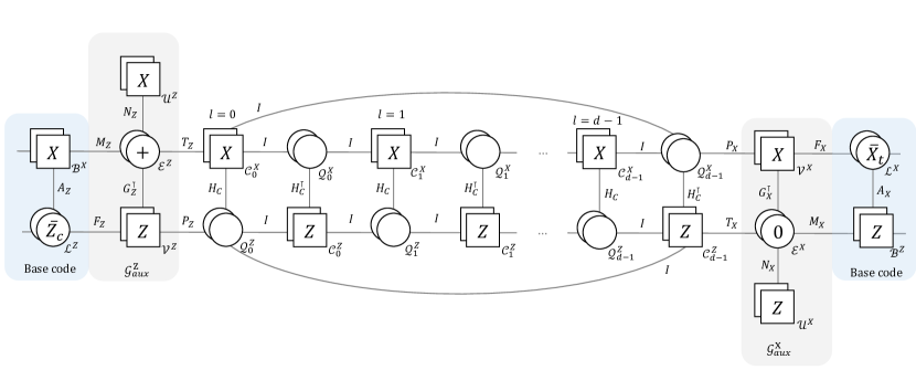
Figure 8: A description of the toric adapter consisting of distance-$d$ toric code connected via edges $T_{Z}$, $P_{Z}$ to auxiliary graphs $\mathcal{G}_{\mathrm{aux}}^{Z}$ and via edges $T_{X}$, $P_{X}$ to $\mathcal{G}_{\mathrm{aux}}^{X}$ to create new code $\mathcal{G}_{\textrm{merge}}$. The auxiliary graphs are built on the support of logicals $\bar{Z}_{c}$ and $\bar{X}_{t}$ in a base LDPC code (shown in blue).

Let $c$ be the control logical qubit and $t$ be the target logical qubit between which we want to implement $\overline{\mathsf{CNOT}}$. Consider their corresponding logical Pauli operators, specifically, $\bar{Z}_{c}$ and $\bar{X}_{t}$. If neither $\bar{Z}_{c}$ nor $\bar{X}_{t}$ contain other logical operators fully in their support, i.e. they are irreducible, then $\bar{Z}_{c}$ and $\bar{X}_{t}$ can be assumed to be pairwise disjoint without loss in generality. This is because any overlapping support between them can be cleaned by multiplying with stabilizers (see Lemma 22 in Appendix). These two logical operators dictate the structure of a new code defined by Tanner graph $\mathcal{G}_{\textrm{merge}}$, shown in Fig. 8. The qubits supporting the $\bar{Z}_{c}$ and $\bar{X}_{c}$ logicals are labelled by sets $\mathcal{L}^{Z}$ and $\mathcal{L}^{X}$. The set of $X(Z)$ stabilizers in the base code that overlap $\bar{Z}_{c}\,(\bar{X}_{t})$ is denoted $\mathcal{B}^{X}$ ($\mathcal{B}^{Z}$). $X(Z)$ stabilizers in $\mathcal{B}^{X}(\mathcal{B}^{Z})$ restricted to the support of $\bar{Z}_{c}(\bar{X}_{t})$ are specified by check matrix $A_{Z}(A_{X})$. The auxiliary graph $\mathcal{G}_{\mathrm{aux}}^{Z}$ consists of $Z$ type checks (labelled $\mathcal{V}^{Z}$), new qubits (labelled $\mathcal{E}^{Z}$) as well as additional $X$ checks (labelled by $\mathcal{U}^{Z}$) to fix gauge degrees of freedom introduced within the additional qubits. The Tanner graph edge describing the support of the new $Z$ checks in $\mathcal{V}^{Z}$ on qubits in $\mathcal{L}^{Z}$ is given by check matrix $F_{Z}$ representing an injection function (as defined in section 2.3). Without loss in generality $F_{Z}$ can assume a form consisting of the identity matrix $I$ and an arbitrary number of additional rows that are all-zero. The Tanner graph edge between $\mathcal{V}^{Z}$ and $\mathcal{E}^{Z}$ is any $G_{Z}^{\top}$, which specifies a graph $G_{Z}$ that allows a low weight perfect matching $M_{Z}$.

The toric code adapter is connected to the base code at $\mathcal{L}^{Z}$ via $\mathcal{G}_{\mathrm{aux}}^{Z}$ by edges described by check matrices $T_{Z}$ and $P_{Z}$, output from $\mathsf{SkipTree}(G^{Z})$. The toric code adapter is similarly attached at $\mathcal{L}^{X}$ via auxiliary graph $\mathcal{G}_{\mathrm{aux}}^{X}$ and additional edges described by check matrices $T_{X}$ and $P_{X}$, output from $\mathsf{SkipTree}(G^{X})$.

5.1.3 Logical circuit

The circuit describing the entire protocol is shown in Fig. 9. We begin with two logical qubits of the LDPC code, $\ket{c}$ and $\ket{t}$ we wish to perform the controlled $\overline{\mathsf{CNOT}}$ between. We also have a prepared toric ancilla state, initialized in the logical state $\ket{+}_{1}\otimes\ket{0}_{2}$.

Figure 9: Circuit describing entire protocol: $(i)$ code deformation, $(ii)$ Dehn twist $\mathsf{CNOT}$, $(iii)$ measuring out the toric ancilla, followed by Pauli corrections $Z^{\,b+c}$ and $X^{a+d}$

The first step $(i)$ is to perform code deformation to merge fault-tolerantly into a new code containing our toric code adapter by adding ancilla qubits initialized suitably and measuring the stabilizers of the new code. One difference from the measurement-based gate set is that here, the goal of code deformation is not to merge into a code containing the logical from our LDPC code as a stabilizer. Instead, the goal is to merge into a new code which contains the ability to perform the gate we want, while maintaining the distance of our LDPC code logical. We prove in the next sections that the number of logical qubits in the merged code is the same as the original LDPC code (Lemma 13), and the distance of the original LDPC code is preserved (Theorem 14). In section 5.2 we elaborate step $(i)$, and explain the reasons behind our choice of starting state and required stabilizer measurements.

In the second step $(ii)$, a logical $\overline{\mathsf{CNOT}}$ applied in the toric code. In section 5.3, we describe how to implement this $\overline{\mathsf{CNOT}}$ on the toric code, introducing and making use of Dehn twists. Notice that one could put any code instead of the toric code in the ancilla as long as it has the ability to implement $\overline{\mathsf{CNOT}}$ and also has at least the same distance $d$ as the original LDPC code. We conjecture other protocols to emerge from this set up, with different choices of more exotic codes connected to the base code using our repetition code adapter, with higher rate to reduce the overhead, and also different choices of gates we want to implement.

The third step $(iii)$ is to measure out the toric code ancilla to unentangle it from the base code. Again, in order to maintain the distance of our code during the process, we measure and apply Pauli corrections based on the measurement outcomes to obtain the $+1$ eigenspace of $\bar{X}_{1}$ and $\bar{Z}_{2}$ operators in the toric code, which resets the toric code ancilla to $\ket{\overline{+0}}$, the state we began with.

This circuit implements $\overline{\mathsf{CNOT}}$ between the control and target on the LDPC code, upto Pauli corrections given by $Z^{\,b+c}$ on the control qubit and $X^{\,a+d}$ on the target qubit, where $a,b$ are the measurement outcomes for $\bar{Z}_{c}\bar{Z}_{1}$ and $\bar{X}_{2}\bar{X}_{t}$ during the merge step $(i)$, and $c,d$ are the measurement outcomes for $\bar{X}_{1}$ and $\bar{Z}_{2}$ during the split step $(ii)$. We prove the correctness of the logical map in section 5.4 (Theorem 16), and verify the fault-distance of the protocol is also preserved (Theorem 17).

The difference between this method and the naive teleportation approach is that in this protocol one does not measure the logical qubit from to the base LDPC code, but rather one entangles an ancilla and then measures out the ancilla again, similar to lattice surgery.

5.1.4 The new code $\mathcal{G}_{\textrm{merge}}$ is gauge-fixed

When we merge into the new code $\mathcal{G}_{\textrm{merge}}$ by measuring the stabilizers of the new code, we want to make sure that no logical qubits get measured in the process, and also check if any gauge degrees of freedom are introduced. In other words, that the total number of logical qubits is preserved i.e. $k^{\prime}=k$.

Lemma 13.

If the original LDPC code $\mathcal{G}$ encodes $k$ qubits, then $\mathcal{G}_{\textrm{merge}}$ encodes $k$ qubits.

Proof.

One can calculate the dimension of the logical space of the new code by calculating the rank of stabilizers and applying the rank-nullity theorem. We defer the detailed calculation to Appendix D.1 and provide a sketch of the argument here. To calculate the rank of $H_{X}^{\prime}$, first partition the check matrix $H_{X}^{\prime}$ into rows corresponding to the different types of $X$ checks in $\mathcal{G}_{\textrm{merge}}$: $\mathcal{B}^{X}$ from the original code, $\mathcal{U}^{Z}$ added to gauge-fix newly introduced qubits in our adapter $\mathcal{G}_{\mathrm{aux}}^{Z}$, and $d$ sets $\mathcal{C}^{X}_{i}$ of checks for $i\in[d]$ from our $d$-layer toric code adapter. The key observations that were useful were the following - the subspace of $X$ checks $\in\mathcal{U}_{Z}$ that originate from cycles in qubits in $\mathcal{E}_{Z}$, has dimension given by the dimension of the cycle basis of the underlying graph $G$. Recall $G$ is defined with $Z$ checks from the set $\mathcal{V}^{Z}$ as its vertices, qubits from set $\mathcal{E}^{Z}$ as its edges and $X$ checks from $\mathcal{U}^{Z}$ as faces or cycles in the graph. The dimension of the cycle basis is known as the cyclomatic number of any connected graph $G(V,E)$ [45], and is equal to $|E|-|V|+1$. Here, dim$(\mathcal{U}^{Z})=|\mathcal{E}_{Z}|-|\mathcal{V}^{Z}|+1$. Secondly, after row-and-column operations, a single redundancy emerges from the rows of the cyclic matrix $H_{C}$ (rank of $d$-bit cyclic code check matrix is $d-1$) as well as $T$. The calculation for $\mathrm{rank}(H_{Z}^{\prime})$ follows analogously, and $k^{\prime}=n^{\prime}-\mathrm{rank}(H_{X}^{\prime})-\mathrm{rank}(H_{Z}^{\prime})$.

∎

5.1.5 Code Distance Is Preserved

We would like the new merged code to have preserve the code distance of the original code.

Theorem 14.

The merged code has distance $d$ if the original code had distance $d$.

Proof.

The argument for distance proceeds symmetrically for both the $\bar{X}_{t}$ and $\bar{Z}_{c}$ distances, so it is sufficient to focus on the $\bar{Z}_{c}$ distance.

Any logical operator has multiple representatives, obtained by multiplying with stabilizers. We want to make sure that new $Z$ stabilizers in $\mathcal{G}_{\textrm{merge}}$ do not clean more support from any $\bar{Z}_{c}$ representative than they add, by considering the effect of multiplication with $Z$ stabilizers that share support with the particular $\bar{Z}_{c}$ representative being inspected. To begin with, consider the $\bar{Z}_{c}$ representative supported on the base code qubits $\mathcal{L}^{Z}$. First consider the cleaning effect of $Z$ stabilizers from the set $\mathcal{V}^{Z}$. These stabilizers have support on qubits in $\mathcal{L}^{Z}$, $\mathcal{Q}^{X}_{0}$ and $\mathcal{E}^{Z}$, with check structure described by check matrices $F_{Z}$ (which is the identity matrix with additional all $0$ rows), permutation $P_{Z}$, and $G^{\top}_{Z}$ (see Fig 10(a)). Given that $G_{Z}$ describes a graph, each row in $G_{Z}$ corresponds to an edge between 2 vertices i.e. every row contains exactly 2 ones. Thus the column sums in its transpose $G_{Z}^{\top}$ are $0$, $\vec{1}G_{Z}^{\top}=0$. In other words, each qubit in $\mathcal{E}^{Z}$ supports an even number of $Z$ checks from $\mathcal{V}^{Z}$, and the product of all these $Z$ checks $\mathcal{H}_{Z}(\vec{1}\in\mathcal{V}^{Z})$ would have its support exactly cancelled on the qubit set $\mathcal{E}^{Z}$. Next, notice that the Tanner graph edges between the checks $\mathcal{V}^{Z}$ and qubits in $\mathcal{L}^{Z}$ and $\mathcal{Q}^{Z}_{0}$ are descibed exactly by the identity matrix $I$ (non-zero rows in $F_{Z}$) and permutation $P_{Z}$, which each have row and column weight $1$. This means for every qubit in $\mathcal{L}^{Z}$ supporting a $Z$ stabilizer in $\mathcal{V}^{Z}$ there exists exactly one corresponding qubit from $\mathcal{Q}^{Z}_{0}$ supporting the same stabilizer, indexed by permutation $P_{Z}$. Thus the entire logical $\bar{Z}_{c}$ can be entirely cleaned from $\mathcal{L}^{Z}$ qubit by qubit and simultaneously moved to $\mathcal{Q}^{Z}_{0}$, as below (shown in Fig 10(a)),

$$Z(\vec{1}\in{\mathcal{L}^{Z}})\;\mathcal{H}_{Z}(\vec{1}\in\mathcal{V}^{Z})=Z(\vec{1}\in\mathcal{Q}^{Z}_{0})$$ (30)

Since the logical is supported on exactly the same number of qubits as before, the distance of $\bar{Z}_{c}$ is preserved under multiplication by $\mathcal{H}_{Z}(\vec{1}\in\mathcal{V}^{Z})$.

Similarly observe that $\vec{1}H_{C}^{\top}=0$, since each of the cyclic repetition code checks is weight $2$. We can further move the support of $\bar{Z}_{c}$ from $\mathcal{Q}^{Z}_{0}$ to $\mathcal{Q}^{Z}_{1}$ by multiplying with all checks from $\mathcal{C}^{Z}_{0}$ to get $Z(\mathcal{Q}^{Z}_{0})\;\mathcal{H}_{Z}(\vec{1}\in\mathcal{C}^{Z}_{0})=Z(\mathcal{Q}^{Z}_{1})$. In fact, since all the dual layers of the toric code have Tanner graph edges described by check matrix $H_{C}^{\top}$, the product of all stabilizers from any set $\mathcal{C}^{Z}_{i}$ for $i\in[d]$ can be used to entirely move the $\bar{Z}_{c}$ logical representative to any of the $d$ layers while preserving the weight of $\bar{Z}_{c}$,

$$Z(\vec{1}\in\mathcal{Q}^{Z}_{i})\;\mathcal{H}_{Z}(\vec{1}\in\mathcal{C}^{Z}_{i})=Z(\vec{1}\in\mathcal{Q}^{Z}_{i+1(\textrm{mod}\,d)})$$ (31)

(a)

(b)

Figure 10: (a) The support of $\bar{Z}_{c}$ can be moved from $\mathcal{L}^{Z}$ to $\mathcal{Q}^{Z}_{0}$, by multiplying all the $Z$ checks from $\mathcal{V}^{Z}$.
(b) Similarly $\bar{X}_{t}$ supported on $\mathcal{L}^{X}$ has an equivalent representative on $\mathcal{Q}^{X}_{d-1}$ in the dual sublayer, obtained by multiplying all the $X$ checks from $\mathcal{V}^{X}$.

The tricky case to prove for is when only a subset of checks from a set $\mathcal{V}^{Z}$ or $\mathcal{C}^{Z}_{i}$ are multiplied to $\bar{Z}_{c}$. Let $\vec{u}\in\mathbb{F}_{2}^{d}$ describe which checks are chosen to multiply to the $\bar{Z}_{c}$ representative, where $u_{b}=1$ indicates the $b$th check is included in the choice of checks to multiply, and $u_{b}=0$ indicates the $b$th check is omitted in the choice. We reasoned above that every time a qubit is cleaned from logical support in $\mathcal{L}^{Z}$, support is gained on another qubit in $\mathcal{Q}^{Z}_{0}$. These checks also potentially add constant weight to qubits in $\mathcal{Q}^{Z}_{0}$, but this does not weaken the minimum distance argument. Hence multiplication by even a subset of checks $u$ from $\mathcal{V}^{Z}$ preserves the $\bar{Z}_{c}$ distance. By similar reasoning, if only a subset $u$ of stabilizers from $\mathcal{C}^{Z}_{i}$, $\mathcal{H}_{Z}(u\in\mathcal{C}^{Z}_{i})$ is multiplied to the representative on $\mathcal{Q}^{Z}_{i}$ or $\mathcal{Q}^{Z}_{i+1}$, then exactly one qubit is added to the support for every qubit cleaned from the logical, as described by the $I$ check matrix on edges between ($\mathcal{C}^{Z}_{i}$,$\mathcal{Q}^{Z}_{i}$) and ($\mathcal{C}^{Z}_{i}$,$\mathcal{Q}^{Z}_{i+1}$). And stabilizers in any other set $\mathcal{C}^{Z}_{w}$ for $w\neq i,i\!+\!1\!\pmod{d}$ certainly do not clean any support from the representative on $\mathcal{Q}^{Z}_{i}$ due to disjoint support, but can only increase the weight of the logical. This proves that the minimum distance of $\bar{Z}_{c}$ is maintained under multiplication by any of the $Z$ stabilizers in $\mathcal{G}_{\textrm{merge}}$, either from $\mathcal{V}^{Z}$ or $\mathcal{C}^{Z}_{i}$ for any $i$.

We can easily extend the above reasoning to argue for the distance of the remaining $\bar{Z}$ logicals of the original LDPC code. The simplest case would be for $\bar{Z}$ logicals that do not intersect $\bar{Z}_{c}$, in other words, have no support on $\mathcal{L}^{Z}$. In this case, the logicals reside in a different part of the code and their weight cannot be reduced by cleaning with newly introduced $Z$ stabilizers in $\mathcal{G}_{\textrm{merge}}$, as they are disjoint. Overlap of $\bar{Z}$ with $\bar{X}_{c}$ is not an issue, since new stabilizers ($\mathcal{V}^{X}$) introduced that have any support on $\mathcal{L}^{X}$ are all $X$-type, multiplication by which only changes $Z$-type operators to $Y$-type, but does not clean their support. The main case to consider is of $\bar{Z}$ logicals which have some arbitrary $s$ overlap on $\mathcal{L}^{Z}$, say $Z(s\in\mathcal{L}^{Z})$ for some $s\neq\vec{1}$, since we have already proved distance for $\bar{Z}_{c}=Z(\vec{1}\in\mathcal{L}^{Z})$. The argument for the cleaning effect from any products of $Z$ stabilizers $\mathcal{H}_{Z}(u\in\mathcal{C}^{Z}_{i})$ or $\mathcal{H}_{Z}(u\in\mathcal{V}^{Z})$ for any selection $u\in\mathbb{F}_{2}^{d}$ of a $Z$-type operator on $\mathcal{L}^{Z}$ did not rely on the actual structure of $\bar{Z}_{c}$. In fact by extension of the reasoning for $\bar{Z}_{c}$, the support of any $Z$-type operator on $\mathcal{L}^{Z}$ would be preserved by multiplication with $Z$ stabilizers from $\mathcal{C}^{Z}_{i}$ and $\mathcal{V}^{Z}$, because of every check simultaneously cleans support and adds the same weight to another set of qubits. Thus the minimum distances of all $Z$-type logicals on the original LDPC code are preserved when merged into the new code.

The $\bar{X}_{c}$ logical corresponding to the same logical qubit as $\bar{Z}_{c}$, would anti-commute with $\bar{Z}_{c}$, and thus overlaps with $\bar{Z}_{c}$ on an odd number of qubits. This is true for any representative of $\bar{Z}_{c}$ (including Eqns 30 and 31). This means $\bar{X}_{c}$ needs to have support on at least one qubit in each of the $d$ layers of the merged code, in order to anticommute with every $\bar{Z}_{c}$ logical representative. This is sufficient to prove that the $X$-distance corresponding to the $\bar{X}_{c}$ is at least equal to the number of layers, $d$.

Next we prove distance for the logical operator $\bar{X}_{t}$ corresponding to the target qubit, which is distinct from the control logical qubit as per the problem set up. $\bar{X}_{t}$ and $\bar{Z}_{c}$ commute, and can have representatives residing in completely disjoint parts of the deformed code. Thus we need a different tactic to prove the distance for $\bar{X}_{t}$. By similar reasoning as earlier, multiplying $\mathcal{H}_{X}(v\in\mathcal{V}^{X})$, the product of all $X$-stabilizers in $\mathcal{V}^{X}$, to the operator $X(\mathcal{L}^{X})$ moves the logical to be entirely supported on the qubit set $\mathcal{Q}^{X}_{d-1}$ (see Fig 10(b)),

$$X(\vec{1}\in{\mathcal{L}^{X}})\;\mathcal{H}_{X}(\vec{1}\in\mathcal{V}^{X})=X(\vec{1}\in\mathcal{Q}^{X}_{d-1})$$ (32)

By similar reasoning as for $\bar{Z}_{c}$, multiplication with all $X$-checks chosen from any of the sets $\mathcal{C}^{X}_{i}$ for $i\in[d]$, would simply move the entire logical operator between layers. Analogous reasoning also follows for multiplication with any subset $u$ of $X$ stabilizers from any of the sets $\mathcal{E}^{X}$ or $\mathcal{C}^{X}_{i}$ for all $i$, which preserve the minimum weight of the $\bar{X}_{t}$ and hence the distance. ∎

Notice the above argument on the code distance did not rely on the $d$ layers in the structure to preserve the code distance for $\bar{Z}_{c}$ or $\bar{X}_{t}$. The $d$ layers are sufficient, though not necessary, to prove minimum distance $d$ for the corresponding anti-commuting logicals $\bar{Z}_{t}$ and $\bar{X}_{c}$, which must overlap with representatives of $\bar{Z}_{c}$ and $\bar{X}_{t}$ in each of the $d$ layers. The $d$ layers will become necessary to preserve the distances of $\bar{Z}_{c}$ or $\bar{X}_{t}$ during the implementation of the unitary circuit.

5.2 Initial Code Deformation step

The standard approach to code deformation into a bigger code that includes the base LDPC code augmented by ancillary qubits is to begin measuring stabilizers of the new code. In order to merge into the new code without reducing the code distance, the initial state on the auxiliary qubits in $\mathcal{E}^{Z}$ and $\mathcal{E}^{X}$ (which will support the auxiliary graphs in $\mathcal{G}_{\textrm{merge}}$) and qubits in sets $\mathcal{Q}^{Z}_{i}$ and $\mathcal{Q}^{X}_{i}$ for $i\in[d]$ (which support the toric code adapter in $\mathcal{G}_{\textrm{merge}}$), needs to be chosen carefully.

First consider the initial state on the auxiliary qubits. The simplest starting state to prepare in practice is a product state, as it simply consists of physical qubits without any encoding. Not all arbitrary product state would be ideal candidate initial states. For instance, initializing $\mathcal{E}^{Z}$ in $\ket{0}^{\otimes|\mathcal{E}^{Z}|}$ with single-qubit $Z$ stabilizers $Z(e_{j}\in\mathcal{E}^{Z})$ or initializing $\mathcal{E}^{X}$ in $\ket{+}^{\otimes|\mathcal{E}^{X}|}$ with single-qubit $X$ stabilizers $X(e_{j}\in\mathcal{E}^{X})$ is not ideal because these stabilizers do not commute with the base code stabilizers ($\mathcal{B}^{X}$ and $\mathcal{B}^{Z}$) of the opposite type they overlap with. The outcome of these stabilizer measurements is no longer deterministic, and hence detector information for base code stabilizer measurements prior to the merging step is lost. To avoid this scenario, instead we introduce single-qubit stabilizers which commute with the base code stabilizers they overlap with, so $X(e_{j}\in\mathcal{E}^{Z})$ for $j\in[|\mathcal{E}^{Z}|]$, and $Z(e_{j}\in\mathcal{E}^{X})$ for $j\in[|\mathcal{E}^{X}|]$, that is, qubits in sets $\mathcal{E}^{Z}$ are initialized as $\ket{+}$ states and qubits in sets $\mathcal{E}^{X}$ are initialized as $\ket{0}$ states.

The initial state of the toric code ancilla state involves some subtleties as well. In section 5.1.5 we have already seen that there are multiple logical representatives for $\bar{Z}_{c}$ and $\bar{X}_{t}$ across the $d$ layers. We do not want to introduce new stabilizers which could clean support from any of these representatives, as that would bring down the minimum distance of $\mathcal{G}_{\textrm{merge}}$. If one chooses to begin with a product state of single-qubit stabilizers, some possibilities can be precluded by inspection: initializing $\mathcal{Q}^{Z}_{i}$ in $\ket{0}$ states with single-qubit $Z$ stabilizers or initializing $\mathcal{Q}^{X}_{i}$ in $\ket{+}$ with single-qubit $X$ stabilizers. This is because if $\mathcal{Q}^{Z}_{i}$ is initialized with single-qubit $Z$ stabilizers, any of these stabilizers cleans support from a $\bar{Z}_{c}$ logical representative $Z(\vec{1}\in\mathcal{Q}^{Z}_{i})$ for any layer $i$ ($\because$ Eqns 30, 31), and reduces the minimum distance of the merged code. In fact, the product of all single qubit $Z$ stabilizers from a set $\mathcal{Q}^{Z}_{i}$ could clean $O(d)$ support or even the entire $\bar{Z}_{c}$ logical. In other words, in the merged subsystem code the dressed distance of the logical would effectively be reduced to $0$. The same issue arises if qubits in $\mathcal{Q}^{X}_{i}$ are initialized with single-qubit $X$ stabilizers, as any of these stabilizers cleans support of $\bar{X}_{t}$ representative $X(\vec{1}\in\mathcal{Q}^{X}_{i})$ and reduces the $X$ distance. For this reason, we are constrained to initialize a state that does not contain operators $Z(s\in\mathcal{Q}^{Z}_{i})$ or $X(s\in\mathcal{Q}^{X}_{i})$ for any $s\in\mathbb{F}_{2}^{d}$, in any layer $i$, within its stabilizer space. One way to ensure this is to instead initialize with single-qubit $X$ and $Z$ stabilizers of the opposite type on these qubits, i.e. $X(e_{j}\in\mathcal{Q}^{Z}_{i})$ and $Z(e_{j}\in\mathcal{Q}^{X}_{i})$ for all $j\in[d]$, in each layer $i$, or in statevector terms, to initialize in the product state $\ket{+}^{\otimes d^{2}}\!\ket{0}^{\otimes d^{2}}$, where all qubit sets $\mathcal{Q}^{Z}_{i}$ as $\ket{+}$ states and $\mathcal{Q}^{X}_{i}$ as $\ket{0}$ states.

While the product state comprising $\ket{+}$ on qubits in $\mathcal{Q}^{Z}_{i}$ and $\ket{0}$ on qubits in $\mathcal{Q}^{X}_{i}$ is straightforward to prepare, a snag is that a threshold for the merging process may not exist, due to the anti-commuting gauge operators present in the deformed subsystem code. When one starts measuring the stabilizers of the toric code to prepare $\mathcal{G}_{\mathrm{toric}}$, the initial single-qubit $X$ checks on $\mathcal{Q}^{Z}_{i}$ anticommute with the new $Z$ toric code checks $\mathcal{C}^{Z}_{i}$ being measured. The anti-commuting operators imply that measurement outcomes are no longer deterministic. The only deterministic measurements are products of stabilizers $\prod_{i=0}^{d-1}Z(e_{j}\in\mathcal{Q}^{Z}_{i})$ and also $\prod_{i=0}^{d-1}X(e_{j}\in\mathcal{Q}^{X}_{i})$, which are $O(d)$ size, thereby not providing enough information for error-correction.

A second approach is to directly add products of single-qubit $Z$ stabilizers or $X$ stabilizers, specifically $\prod_{i=0}^{d-1}Z(e_{j}\in\mathcal{Q}^{Z}_{i})$ and $\prod_{i=0}^{d-1}X(e_{j}\in\mathcal{Q}^{X}_{i})$ to the stabilizer group for the initial state. These are also representatives of $\bar{Z}_{2}$ and $\bar{X}_{1}$ on the toric code, so this means initializing directly in the $\ket{\overline{+0}}$ logical state. The qubits are not in a product state but rather in a highly entangled state belonging to the toric code codespace. We decide to blackbox the preparation of the toric code state. Note, even for choosing a suitable state within the toric codespace, one can rule out the $+1$ eigenspaces of both $\bar{Z}_{1}$ and $\bar{X}_{2}$ logicals, because once measured, the logical operators are added to the stabilizer group and the newly added stabilizers ($\bar{Z}_{1}$, $\bar{X}_{2}$ in this scenario) would clean the support of $\bar{Z}_{c}$ or $\bar{X}_{t}$ and reduce the distance of our merged code. This reduces the feasible subspace for initializing the toric code ancilla, from $4$ states to exactly one codestate, $\ket{\overline{+0}}$. Methods to prepare such a state exist, for example by simply measuring the logical operators $\bar{X}_{1}$ and $\bar{Z}_{2}$ (using gauging measurement [31], sec 2.3 or homomorphic measurements [55]) to prepare their simultaneous $+1$ eigenstate, applying Pauli corrections where necessary.

It is possible that the product state $\ket{+}^{\otimes d^{2}}\!\ket{0}^{\otimes d^{2}}$ on the toric code is effective for small-size demonstrations, despite the code deformation step lacking a threshold, since errors can still be effectively detected. For a scheme applicable in the asymptotic regime, we defer to using $\ket{\overline{+0}}$ as the initial state in the toric code adapter.

With the auxiliary qubits and preprepared toric codestate initialized as described, code deformation takes place by measuring stabilizers of the new code $\mathcal{G}_{\textrm{merge}}$ (Tanner graph in Fig. 8). At the end of the protocol during the split step $(iii)$, we measure the initial stabilizers again, that is, stabilizers of the base LDPC code, single-qubit $X$ stabilizers on $\mathcal{E}^{Z}$, single-qubit $Z$ stabilizers on $\mathcal{E}^{X}$ and measure the logical operators $\bar{X}_{1}$ and $\bar{Z}_{2}$ on the toric code $\mathcal{G}_{\mathrm{toric}}$, applying corrections to reset the toric code to $\ket{\overline{+}}\otimes\ket{\overline{0}}$.

5.3 Code Evolution During The Unitary Circuit

Once we have deformed to the new code, transversal physical $\mathsf{CNOT}$ gates are applied within each layer of the toric code, between qubits in sets $\mathcal{Q}^{Z}_{i}$ and $\mathcal{Q}^{X}_{i}$, as shown in Figure 11. In each layer $i$, the transversal $\mathsf{CNOT}$s act between corresponding qubits sharing the same index $j$. Let gates between two qubit sets in layer $i$ be described as ${\mathsf{CNOT}}(\mathcal{Q}^{Z}_{i},\mathcal{Q}^{X}_{i})$ where we use the shorthand ${\mathsf{CNOT}}(\mathcal{A},\mathcal{B})$ to denote transversal physical $\mathsf{CNOT}$ gates between qubits in ordered sets $\mathcal{A}=\{a_{j}\}$ and $\mathcal{B}=\{b_{j}\}$ for $j\in[d]$,

$${\mathsf{CNOT}}(\mathcal{A},\mathcal{B})=\prod_{j=0}^{d-1}{\mathsf{CNOT}}_{a_{j}b_{j}}$$ (33)

(Here the unit vector $e_{j}$ describing qubit index is additionally indexed by the set containing the qubit)

The overall operation can be written as a product of transversal gates from all layers $i\in[d]$,

$$\prod_{i=0}^{d-1}{\mathsf{CNOT}}(\mathcal{Q}^{Z}_{i},\mathcal{Q}^{X}_{i})$$ (34)

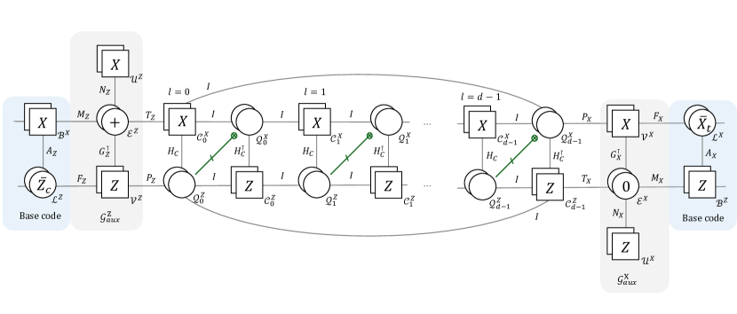
Figure 11: Transversal physical $\mathsf{CNOT}$s applied with qubits in sets $\mathcal{Q}^{Z}_{i}$ as control qubits and $\mathcal{Q}^{X}_{i}$ as target qubits, in each layer $i$.

Since all the qubit sets $\mathcal{Q}^{Z}_{i}$ and $\mathcal{Q}^{X}_{i}$ are disjoint, these physical $\mathsf{CNOT}$ gates can be implemented in parallel. Note that each set of transversal $\mathsf{CNOT}$s effectively takes place within a single layer of the toric code. This parallelized $\mathsf{CNOT}$ scheme has constant time overhead, and provides a speedup from conventional round-robin gate schemes which are $O(d)$ depth and take place gradationally over multiple rounds consisting of transversal physical gates.

5.3.1 Notation on permutations

Before we proceed, we find it relevant to establish convention to distinguish between permutations on (qu)bits and checks for any one type of stabilizer for a CSS quantum code, or any classical code. Consider a set $\mathcal{C}$ of checks, and set $\mathcal{Q}$ of (qu)bits. An individual check indexed $j\in[|\mathcal{C}|]$ is written as $e_{j}\in\mathbb{F}_{2}^{|\mathcal{C}|}$, where $e_{j}$ is the binary row vector with a $1$ only in the $j^{\textrm{th}}$ position. A qubit indexed $j\in[|\mathcal{Q}|]$ is written as $e_{j}^{\top}\in\mathbb{F}_{2}^{|\mathcal{Q}|}$. Let the check matrix $A\in\mathbb{F}_{2}^{|\mathcal{C}|\times\mathcal{Q}|}$ describe the collection of edges in the Tanner graph between individual checks from set $\mathcal{C}$ and qubits from $\mathcal{Q}$, where this collection itself can be viewed as an edge in the abstract Tanner graph between sets of qubits and checks. Use row vector $u\in\mathbb{F}_{2}^{|\mathcal{C}|}$ to denote selections of checks from $\mathcal{C}$, and use column vector $v^{\top}\in\mathbb{F}_{2}^{|\mathcal{Q}|}$ to denote selections of (qu)bits from $\mathcal{Q}$, where $1$ indicates if the (qu)bit or check is present in the choice. Then $uA$ is a column vector that gives the (qu)bits supporting checks in $u$, and $Av^{\top}$ gives the syndrome corresponding to bitstring $v^{\top}$. Permuting checks in $\mathcal{C}$ under $\pi:u\rightarrow u\pi$ is equivalent to left-multiplying $A$ by $\pi$, since $(u\pi)A=u(\pi A)$. In order to keep the product $uA$ (bits supporting checks $u$) invariant, a permutation on checks by $\pi$ needs to be accompanied by left-multiplication of $A$ by $\pi^{\top}$ and vice-versa, as $uA=(u\pi)(\pi^{\top}A)$ $(\because\pi\pi^{\top}=I)$.

Next, note that permuting qubits in $\mathcal{Q}$ under permutation $\sigma:v\rightarrow v\sigma$ or equivalently $v^{\top}\rightarrow(v\sigma)^{\top}=\sigma^{\top}v^{\top}$ transforms the syndrome the same way as right-multiplying $A$ by $\sigma^{\top}$ instead, since $A(\sigma^{\top}v^{\top})=(A\sigma^{\top})v^{\top}$. Again, it follows that to keep the syndrome invariant, a right-multiplication of $A$ by $\sigma$ must be accompanied by permutation $\sigma$ on qubits $v$ and vice-versa, since $Av^{\top}\!=(A\sigma)(\sigma^{\top}v^{\top})\;(\because\sigma\sigma^{\top}\!\!=\!I)=(A\sigma)(v\sigma)^{\top}$.

Overall, the effective transformation on edge $A$ of the Tanner graph, for check structure and syndrome to remain invariant after permutation $\pi$ on checks and $\sigma$ on qubits, is $A\longrightarrow\pi^{\top}A\,\sigma$, as shown in Figure 12. Conversely, if the edge $A$ transforms as $A\longrightarrow\pi^{\top}A\,\sigma$, then to preserve check structure and syndrome (and in the case where the syndrome is $0$, to remain in the same codespace), permutations $\pi$ on checks and $\sigma$ on qubits need to be applied.

Figure 12: Permuting qubits and checks: $A\longrightarrow\pi^{\top}A\,\sigma$

5.3.2 Tracking stabilizer evolution

We examine the effect of each set of transversal $\mathsf{CNOT}$s on the quantum state initialized in the codespace of $\mathcal{G}_{\textrm{merge}}$, by describing their action on the stabilizer tableau [56]. First consider the action of the circuit on $X$-type stabilizers, as $\mathsf{CNOT}$ gates do not mix $X$ and $Z$ type operators. The action on $Z$-type stabilizers proceeds similarly, with controls and targets exchanged. Consider the $i\!=\!0$ layer of the toric code. $X$-stabilizers from the set $\mathcal{C}^{X}_{0}$ are transformed as

$$\begin{pmatrix}T_{Z}&H_{C}&I\end{pmatrix}\;\xrightarrow{\mathsf{CNOT}(\mathcal{Q}_{0}^{Z},\mathcal{Q}_{0}^{X})}\; \begin{pmatrix}T_{Z}&H_{C}&I+H_{C}\end{pmatrix}$$

$$= \begin{pmatrix}T_{Z}&H_{C}&C\end{pmatrix}$$ (35)

In the above we used the simple observation that $I+H_{C}=C$, where $C$ refers to the cyclic shift matrix by 1 with entries $\ket{j}\bra{j+1}{\pmod{d}}$. Thus Eqn 5.3.2 shows that applying physical $\mathsf{CNOT}$s implements a transformation $I\rightarrow C$ on the edge between $\mathcal{C}^{Z}_{0}$ and $\mathcal{Q}^{X}_{0}$ in the Tanner graph. Following the reasoning in section 5.3.1, in order to preserve the codespace a permutation $\sigma_{0}$ (now additionally indexed $0$ to indicate layer $0$) is applied to qubits $v$ in $\mathcal{Q}^{X}_{0}$ such that the desired net transformation of edge $I\rightarrow C\sigma_{0}=I$, which implies $\sigma_{0}=C^{-1}$. Equivalently, apply $\sigma_{0}^{\top}$ to $v^{\top}$ where $\sigma_{0}^{\top}\!=(C^{-1})^{\top}\!=C\;(\because C$ is unitary$)$. Applying the permutation, we get $Ce_{j}^{\top}=e_{j+1}^{\top}$ for all $j\in[d]$ and so each qubit indexed $j$ is relabelled with index $j+1$. Thus transversal physical $\mathsf{CNOT}$s followed by $C^{-1}$ on qubits in $\mathcal{Q}^{X}_{0}$ preserve the stabilizer space of $X$ stabilizers in $\mathcal{C}^{X}_{0}$.

Meanwhile, $Z$-stabilizers from the set $\mathcal{C}_{0}^{Z}$ transform under action of these transversal $\mathsf{CNOT}$s to

$$\begin{pmatrix}I&H_{C}^{\top}&I\end{pmatrix}\;\xrightarrow{\mathsf{CNOT}(\mathcal{Q}_{0}^{Z},\mathcal{Q}_{0}^{X})}\; \begin{pmatrix}I+H_{C}^{\top}&H_{C}^{\top}&I\end{pmatrix}$$

$$= \begin{pmatrix}C^{-1}\quad\;&H_{C}^{\top}&I\end{pmatrix}$$ (36)

Here the transversal $\mathsf{CNOT}$s apply a cyclic shift $C^{-1}$ to the Tanner graph edge $I$ between $Z$ check set $\mathcal{C}^{Z}_{0}$ and the qubit set $\mathcal{Q}^{Z}_{0}$. The transformation on check matrix $I\rightarrow\pi_{0}^{\top}C^{-1}=I$ must be accompanied either by a permutation $\pi_{0}=C^{-1}$ on checks in $\mathcal{C}^{Z}_{0}$, or $C$ on qubits in $\mathcal{Q}^{Z}_{0}$. Since the labels for qubits in $\mathcal{Q}^{Z}_{0}$ are already fixed by $P_{Z}$, this time we incorporate a permutation $\pi_{0}$ into the set $\mathcal{C}^{Z}_{0}$ of $Z$ checks.

One can verify that the remaining edge in layer $i\!=\!0$, the edge between qubits from $\mathcal{Q}^{X}_{0}$ (permuted by $\sigma_{0}=C^{-1}$) and checks in $\mathcal{C}^{Z}_{0}$ (permuted by $\pi_{0}=C^{-1}$), remains invariant under these permutations. The overall transformation on edge $(\mathcal{Q}^{X}_{0},\mathcal{C}^{Z}_{0})$ is given by

$$H_{C}^{\top}\longrightarrow\; (C^{-1})^{\top}H_{C}^{\top}\,C^{-1} \because A\rightarrow\pi^{\top}A\,\sigma$$ ()

$$=\; C\,(I+C^{-1})\,C^{-1}=\,CC^{-1}+\,CC^{-1}C^{-1}=\;I+C^{-1}=\;H_{C}^{\top}$$ (37)

In the above, we used the fact that $H_{C}^{\top}=I+C^{-1}$ and $C^{\top}\!\!=C^{-1}$ because $C$ is unitary.

To summarize, physical $\mathsf{CNOT}(\mathcal{Q}^{Z}_{0},\mathcal{Q}^{X}_{0})$ followed by permutations $\sigma_{0}$ on qubits in $\mathcal{Q}^{X}_{0}$ and $\pi_{0}$ on $Z$-checks in $\mathcal{C}^{Z}_{0}$, preserve all original Tanner graph edges belonging to the $0^{\textrm{th}}$ layer of $\mathcal{G}_{\textrm{merge}}$, where

$$\sigma_{0}=C^{-1}\;\text{ and }\;\pi_{0}=C^{-1}.$$ (38)

Qubits $\mathcal{Q}^{X}_{0}$ and checks $\mathcal{C}^{Z}_{0}$ also have outgoing edges to $\mathcal{C}^{X}_{1}$ and $\mathcal{Q}^{Z}_{1}$ in the primal sublayer of next layer, $i=1$, described by check matrices equal to the identity matrix $I$ as per the definition of $\mathcal{G}_{\mathrm{toric}}$ (see Fig 11). To ensure this check structure remains preserved even after permutations $\sigma_{0}$ and $\pi_{0}$ on $\mathcal{Q}^{X}_{0}$ and $\mathcal{C}^{Z}_{0}$, we need to apply adjustment permutations $\pi_{1}^{\prime}$ on check set $\mathcal{C}^{X}_{1}$ and $\sigma_{1}^{\prime}$ on qubit set $\mathcal{Q}^{Z}_{1}$. Here we have denoted permutations in the primal sublayers with a prime^′. Specifically we want $\pi_{1}^{\prime}$ on $\mathcal{C}^{X}_{1}$ such that $I\rightarrow(\pi^{\prime}_{1})^{\top}I\,\sigma_{0}=I$ and also $\sigma_{1}^{\prime}$ on $\mathcal{Q}^{Z}_{1}$ such that $I\rightarrow\pi^{\top}_{0}I\,\sigma_{1}^{\prime}=I$. This is satisfied when $\pi_{1}^{\prime}=\sigma_{0}$ and $\sigma_{1}^{\prime}=\pi_{0}$. From Eqn 38 we know $\sigma_{0}=\pi_{0}=C^{-1}$. Therefore, permutations $\pi_{1}^{\prime}$ on checks in $\mathcal{C}^{X}_{1}$ and $\sigma_{1}^{\prime}$ on qubits in $\mathcal{Q}^{Z}_{1}$, restore the edges connecting layers $i\!=\!0$ and $i\!=\!1$ of the toric code, where

$$\sigma_{1}^{\prime}=C^{-1}\;\text{ and }\;\pi_{1}^{\prime}=C^{-1}.$$ (39)

By extension of the same reasoning, it is clear that in order to preserve the edges $I$ connecting dual sublayer $i$ and primal sublayer $i+1{\pmod{2}}$, any permutations $\sigma_{i}$ on $\mathcal{Q}^{X}_{i}$ qubits and $\pi_{i}$ on $\mathcal{C}^{Z}_{i}$ checks in layer $i$ necessitate permutations $\pi_{i+1}^{\prime}$ on $\mathcal{C}^{X}_{i}$ checks and $\sigma_{i+1}^{\prime}$ on $\mathcal{Q}^{Z}_{i}$ qubits in the next layer $i+1$, given by:

$$\sigma_{i+1}^{\prime}=\pi_{i}\;\text{ and }\;\pi_{i+1}^{\prime}=\sigma_{i}$$ (40)

Returning to the stabilizer tableau, we see that $X$-stabilizers $\in\mathcal{C}^{X}_{i}$ in layers $i=1...d-1$ evolve under transversal $\mathsf{CNOT}$s in layer $i$ in their local of frame of reference (i.e. with respect to qubits from $\mathcal{Q}^{X}_{i},\mathcal{Q}^{X}_{i-1},\mathcal{Q}^{Z}_{i}$ in their support prior to any permutations) in a manner similar to $X$ stabilizers in $\mathcal{C}^{X}_{0}$ (Eqn 5.3.2),

$$\begin{pmatrix}I&H_{C}&I\end{pmatrix}\;\xrightarrow{\mathsf{CNOT}(\mathcal{Q}^{Z}_{i},\mathcal{Q}^{X}_{i})}\; \begin{pmatrix}I&H_{C}&I+H_{C}\end{pmatrix}$$

$$= \begin{pmatrix}I&H_{C}&C\end{pmatrix}$$ (41)

This implies that the net permutation $\sigma_{i}$ required on qubits in $\mathcal{Q}^{X}_{i}$ would need to undo the shift $C$ introduced by the transversal $\mathsf{CNOT}$ gates in the $i$th layer, in addition to any permutation $\pi_{i}^{\prime}$ on checks in $\mathcal{C}^{X}_{i}$. The desired net transformation of edge $I\rightarrow(\pi_{i}^{\prime})^{\top}C\sigma_{i}=I$ which implies $\sigma_{i}=C^{-1}\pi_{i}^{\prime}=C^{-1}\sigma_{i-1}\;(\because\text{ Eqn~{}}\ref{eqn-perm-diff-layers})$. This decouples the recurrence relation in Eqn 40 to give a simple recurrence relation for $\sigma_{i}$ for which we have already seen the base case, $\sigma_{0}=C^{-1}$ for layer $0$. Solving, we get the closed form $\sigma_{i}=(C^{-1})^{i}C^{-1}=C^{-i-1}$. Thus the net permutation $\sigma_{i}$ on qubits $\mathcal{Q}^{X}_{i}$ in each layer is given by $C^{-i-1}$. The permutations $\pi_{i}$ on checks in $\mathcal{C}^{Z}_{i}$ follow by tracking evolution of $Z$ stabilizers $\in\mathcal{C}^{Z}_{i}$. This completes the set of permutations in the dual sublayers. Applying Eqn 40 we also obtain closed forms for permutations $\sigma_{i}^{\prime}$ and $\pi_{i}^{\prime}$ in the primal sublayers. In summary,

$$\sigma_{i}=C^{\,-i-1}\; \text{ and }\;\pi_{i}=C^{\,-i-1}$$ (42)

$$\sigma_{i}^{\prime}=C^{\,-i}\quad\, \text{ and }\;\pi_{i}^{\prime}=C^{\,-i}$$ (43)

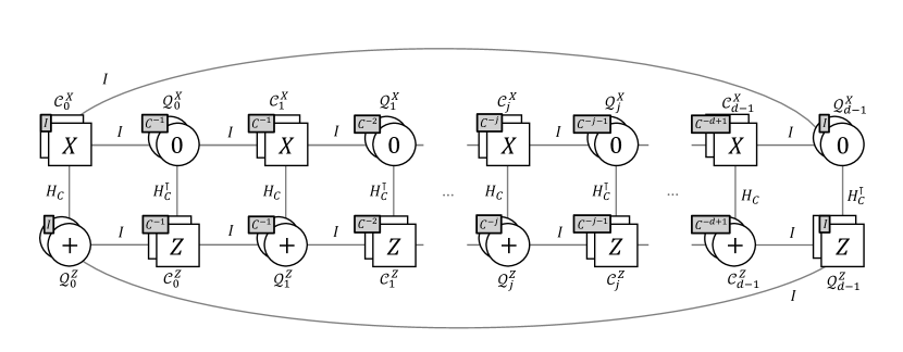
Figure 13: Cyclic permutations on qubits and checks to restore the system back to the original codespace after applying physical $\mathsf{CNOT}$ gates.

The required permutations on all sets of qubits and checks in each layer to remain within the codespace are shown in Figure 13. Note as a result of these permutations $\sigma_{i}$ on qubits in $\mathcal{Q}^{X}_{i}$, the targets for transversal $\mathsf{CNOT}$s are shifted by one index in each successive layer, shifted in total by $i$ for layer $i$. Instead of tranversal $\mathsf{CNOT}$s being implemented between qubit $j$ as control and qubit $j$ as target for all $j$, now the transversal gates act between qubit $j$ control and qubit $j\!+\!1$ as target in layer $1$, qubit $j\!+\!2$ as target in layer $2$ and so on till qubit $j\!+\!i\pmod{d}$ as target in layer $i$.

In the toric code, permutations on qubits and checks (due to Eqns 5.3.2 and 5.3.2) have a geometric interpretation - the plaquettes ($Z$ stabilizers) and qubits on horizontal edges of the plaquette, are shifted by one unit cell with respect to the previous layer, along a non-trivial loop in the dual space defined by qubits supported on $\mathcal{Q}^{X}_{0}$. The combined operation of transversal $\mathsf{CNOT}$ gates followed by permutations determined by $\{\sigma_{i},\pi_{i}\}$ preserve the toric code codespace and hence belong to the normalizer group of stabilizers of $\mathcal{G}_{\mathrm{toric}}$. In the following section we prove that this executes the logical $\overline{\mathsf{CNOT}}$ map. Existing literature [35, 34, 36] refers to these as gates via Dehn twists. Dehn twists are useful to move logical qubits in storage and implement a logical two-qubit Clifford by twisting a toric code along a boundary and applying physical gates acting on pairs of qubits over increasing distances. Dehn twists are parallelizable although at the cost of a similar overhead to topological codes.

In the following section we prove a useful lemma to verify correctness of the logical action, and in section 5.4, we extend this useful result from topological code literature to be adapted efficiently to an arbitrary LDPC code. Unlike our previous results, no expansion properties are required from the LDPC code to execute this gate fault-tolerantly. However, the overhead of this more general approach is higher, $O(d^{2})$, similar to [27].

5.3.3 $\mathsf{CNOT}$ Logical action via Dehn Twists on the toric code

We first state and verify the logical action for Dehn Twists on the toric code in Lemma 15, through the lens of our notation.

Lemma 15 ($\overline{\mathsf{CNOT}}$ Logical action via Dehn Twists).

Consider the toric code, a $[[2d^{2},2,d]]$ CSS code described by the Tanner graph $\mathcal{G}_{\mathrm{toric}}$ with qubits and checks labelled as in Definition 12. A $\overline{\mathsf{CNOT}}_{12}$ gate can be performed between its two logical qubits (w.l.o.g. $1$ is chosen to be the control qubit) using the following circuit

$$\overline{\mathsf{CNOT}}_{12}=\;\prod_{i=0}^{d-1}\,\mathsf{\Gamma}_{i}^{\prime}(\mathcal{Q}^{Z}_{i})\;\mathsf{\Gamma}_{i}(\mathcal{Q}^{X}_{i})\;{\mathsf{CNOT}}(\mathcal{Q}^{Z}_{i},\mathcal{Q}^{X}_{i})$$ (44)

where $\mathsf{\Gamma}_{i}(\mathcal{A})$ is a unitary corresponding to permutations by $C^{-i-1}$ on qubits $e_{j}\in\mathcal{A}$, and $\mathsf{\Gamma}_{i}^{\prime}(\mathcal{A})$ is a unitary corresponding to permutations by $C^{-i}$ on qubits $e_{j}\in\mathcal{A}$, as derived in sec 5.3.2
and ${\mathsf{CNOT}}(\mathcal{A},\mathcal{B})$ is shorthand for transversal $\mathsf{CNOT}$ gates between qubits in ordered sets $\mathcal{A}$ and $\mathcal{B}$, $|\mathcal{A}|=|\mathcal{B}|$, defined as in Eqn 33.

Proof.

The desired action of $\overline{\mathsf{CNOT}}_{12}$ on the Pauli logicals of the toric code is given by

$$\bar{X}_{1} \rightarrow\bar{X}_{1}\bar{X}_{2}$$ (45a)

$$\bar{Z}_{1} \rightarrow\bar{Z}_{1}$$ (45b)

$$\bar{X}_{2} \rightarrow\bar{X}_{2}$$ (45c)

$$\bar{Z}_{2} \rightarrow\bar{Z}_{1}\bar{Z}_{2}$$ (45d)

Consider the initial logical operators of the attached toric code ancilla system, before the circuit described by Eqn (44) is implemented. In the standard form, the logical representatives of the toric code are tensored $X$ and $Z$ operators supported on qubits along each topologically non-trivial loop in the original lattice underlying the compact description Tanner graph $\mathcal{G}_{\mathrm{toric}}$,

$$\bar{X}_{1} =\prod_{i=0}^{d-1}X({e}_{0}\in\mathcal{Q}_{i}^{Z})$$ (46a)

$$\bar{X}_{2} =X(\vec{1}\in\mathcal{Q}^{X}_{0})$$ (46b)

$$\bar{Z}_{1} =Z(\vec{1}\in\mathcal{Q}^{Z}_{0})$$ (46c)

$$\bar{Z}_{2} =\prod_{i=0}^{d-1}Z({e}_{0}\in\mathcal{Q}^{X}_{i})$$ (46d)

In order to see why Eqn 46a holds, note that $|\bar{X}_{1}\cap\bar{Z}_{1}|\equiv\phi_{1}$ is odd, and is at least 1. This implies $\phi_{1}$ qubits in each set $\mathcal{Q}^{Z}_{i}$ fully supporting a $\bar{Z}_{1}$ representative also supports part of the $\bar{X}_{1}$ representative. We can multiply the weight-2 cyclic code $X$ checks in $\mathcal{C}^{X}_{i}$ to clean even-sized support from $\phi_{1}$ to obtain a form of the logical where each set $\mathcal{Q}^{Z}_{i}$ supports exactly one qubit in $\bar{X}_{1}$. The cyclic code stabilizers in $\mathcal{C}^{X}_{i}$ can also move this single-qubit support within $\mathcal{Q}^{Z}_{i}$ such that $\bar{X}_{1}$ representative has support on the first qubit $e_{0}$ in every layer.

It is trivial to see that logical $\bar{X}_{2}$ is unchanged under Dehn twist circuit in Eqn 44. Recall $\bar{X}_{2}$, supported on all the qubits in set $\mathcal{Q}^{X}_{0}$, is entirely contained within the first ($i\!=\!0$) layer and so it is sufficient to consider $\mathsf{CNOT}(\mathcal{Q}^{Z}_{0},\mathcal{Q}^{X}_{0})$ implemented in layer $0$ alone. These gates are controlled on qubits $e_{j}\in\mathcal{Q}^{Z}_{0}$ for all $j\in[|\mathcal{Q}^{Z}_{0}|]$, and are targeted on $e_{j}\in\mathcal{Q}^{X}_{0}$. Each physical $\mathsf{CNOT}$ gate leaves an $X$-type operator on its target qubit unchanged, $X(e_{j}\in\mathcal{Q}^{X}_{0})\rightarrow X(e_{j}\in\mathcal{Q}^{X}_{0})$. The transversal $\mathsf{CNOT}$s leave any $X$-type operator residing on qubits in set $\mathcal{Q}^{X}_{0}$ unchanged.

Similarly, $\bar{Z}_{1}$ resides on all the qubits in set $\mathcal{Q}_{0}^{Z}$, and is unchanged under action of transversal physical $\mathsf{CNOT}$s, as the $Z$ operators supported on control qubits of a physical $\mathsf{CNOT}$ remain invariant.

Next we look at $\bar{X}_{1}$, specifically considering the representative in Eqn 46a. This representative resides on one qubit from each of the $d$ layers, and thus will be affected by the first physical $\mathsf{CNOT}$ gate in each layer. Each physical $\mathsf{CNOT}$ maps $X(e_{0}\in\mathcal{Q}^{Z}_{i})\rightarrow X(e_{0}\in\mathcal{Q}^{Z}_{i})X(e_{0}\in\mathcal{Q}^{X}_{i})$ for all $i\in[d]$. Next, we apply permutation $C^{-i}$ on $\mathcal{Q}^{X}_{i}$ in each layer $i$. Under permutation by $C^{-i}$, each qubit $e_{0}^{\top}$ in $\mathcal{Q}^{X}_{i}$ is mapped to $e_{i}^{\top}$, leaving the resulting operator $X(e_{0}\in\mathcal{Q}^{Z}_{i})X(e_{i}\in\mathcal{Q}^{X}_{i})$. Recall as per the Tanner graph $\mathcal{G}_{\mathrm{toric}}$, each $X$ check in any set $\mathcal{C}^{X}_{i}$ can clean exactly one qubit from layer $i$ and add the exactly the same support to layer $i\!-\!1$. All the qubits $e^{\top}_{i}$ can be moved by stabilizer multiplication $\prod_{i=0}^{d}\prod_{i^{\prime}=0}^{i}(e_{i^{\prime}}\in\mathcal{C}^{X}_{i})$ to create $\sum_{i=0}^{d-1}e_{i}=\vec{1}$ support on $\mathcal{Q}^{X}_{0}$. The resulting operator is $X(e_{0}\in\mathcal{Q}^{Z}_{i})X(\vec{1}\in\mathcal{Q}^{X}_{0})=\bar{X}_{1}\bar{X}_{2}$. This verifies the logical map $\bar{X}_{1}\rightarrow\bar{X}_{1}\bar{X}_{2}$.

The last logical to verify the action of the circuit in Eqn 44 is the $\bar{Z}_{2}$ logical. We pick a representative of $\bar{Z}_{2}$ which has exactly single qubit support in each of the $d$ layers, which we choose without loss of generality to be the first qubit in all qubit sets $\mathcal{Q}_{i}^{X}$. Since $Z$ operators flow from the target to the control of physical $\mathsf{CNOT}$s, each physical gate maps $Z(e_{0}\in\mathcal{Q}^{X}_{i})\rightarrow Z(e_{0}\in\mathcal{Q}^{Z}_{i})Z(e_{0}\in\mathcal{Q}^{X}_{i})$ for all $i\in[d]$. After permutations $C^{-i-1}$ to qubits in sets $\mathcal{Q}^{Z}_{i}$ in each layer, each qubit $e_{0}^{\top}$ in $\mathcal{Q}^{Z}_{i}$ is mapped to $e_{i+1}^{\top}$, leaving the resulting operator $Z(e_{i+1}\in\mathcal{Q}^{Z}_{i})Z(e_{0}\in\mathcal{Q}^{X}_{i})$. Note that the cyclic shift $i+1$ is modulo $d$. For any pair of qubits in different layers, $i_{1}$ and $i_{2}$, for $i_{1}\neq i_{2}$, $e_{i_{1}+1}\neq e_{i_{2}+1}$, and further, for any layer $i\in[d]$, the qubit indexed ${i+1}\pmod{d}$ in $\mathcal{Q}^{Z}_{i}$ supports the resulting operator. Once again it is possible to multiply $Z$ stabilizers from $\mathcal{C}^{Z}_{i}$ to move the logical support qubit by qubit from all layers $i$ to layer $i\!=\!0$, to obtain resulting operator $Z(\vec{1}\in\mathcal{Q}^{Z}_{i})Z(e_{0}\in\mathcal{Q}^{X}_{i})=\bar{Z_{1}}\bar{Z_{2}}$. This verifies the logical map $\bar{Z}_{2}\rightarrow\bar{Z}_{1}\bar{Z}_{2}$.

The last thing to note for correctness of logical action is that the Dehn twist circuit described preserves the stabilizer space. Permutations $C^{-i}$ on qubits and checks in the primal sublayers and permutations $C^{-i-1}$ on qubits and checks in the dual sublayers restore the original Tanner graph edges of $\mathcal{G}_{\textrm{merge}}$ after physical $\mathsf{CNOT}$s, as shown in section 5.3.2. ∎

5.4 $\mathsf{CNOT}$ Logical action on arbitrary LDPC codes using unitary adapter

Once we have measured into the merged code, the $\bar{X}_{t}$ logical from the base code has additional logical representatives which can be obtained by multiplying with stabilizers from the merged code. This provides an avenue for effectively ‘moving’ logical information from the base code to the ancilla by entangling the two systems, which is complementary to teleportation-based techniques and does not require a final measurement on the base code, but rather on the adapter.

Theorem 16.

Consider an arbitrary $[[n,k,d]]$ CSS LDPC code. Let $c$ and $t$ be any two logical qubits in this code. We assume w.l.o.g. that $\bar{Z}_{c}$ and $\bar{X}_{t}$ are assumed to be pairwise disjoint (see Lemma 22 in Appendix). Let $\mathcal{G}_{\textrm{merge}}$ be the obtained code after merging with the toric code adapter using auxiliary graphs $\mathcal{G}_{\mathrm{aux}}^{Z}\cup\mathcal{G}_{\mathrm{toric}}\cup\mathcal{G}_{\mathrm{aux}}^{X}$. The circuit defined below implements the desired targeted logical $\overline{\mathsf{CNOT}}$ between the quantum LDPC logical qubits $c$ and $t$.

$$\overline{\mathsf{CNOT}}_{c\,t}=\,\;\;\prod_{i=0}^{d-1}\,\mathsf{\Gamma}_{i}^{\prime}(\mathcal{Q}^{Z}_{i})\;\mathsf{\Gamma}_{i}(\mathcal{Q}^{X}_{i})\;{\mathsf{CNOT}}(\mathcal{Q}^{Z}_{i},\mathcal{Q}^{X}_{i})$$ (47)

where $\mathsf{\Gamma}_{i}(\mathcal{A})$ is a unitary corresponding to permutations by $C^{-i-1}$ on qubits $e_{j}\in\mathcal{A}$, and $\mathsf{\Gamma}_{i}^{\prime}(\mathcal{A})$ is a unitary corresponding to permutations by $C^{-i}$ on qubits $e_{j}\in\mathcal{A}$, and ${\mathsf{CNOT}}(\mathcal{A},\mathcal{B})$ is shorthand for transversal gates between two ordered sets of qubits $\mathcal{A}$ and $\mathcal{B}$ defined in Eqn 33.

Proof.

The desired logical action for the $\overline{\mathsf{CNOT}}_{ct}$ gate is to conjugate the Pauli logicals as follows:

$$\bar{X}_{c} \rightarrow\bar{X}_{c}\bar{X}_{t}$$ (48a)

$$\bar{Z}_{c} \rightarrow\bar{Z}_{c}$$ (48b)

$$\bar{X}_{t} \rightarrow\bar{X}_{t}$$ (48c)

$$\bar{Z}_{t} \rightarrow\bar{Z}_{c}\bar{Z}_{t}$$ (48d)

$\bar{X}_{c}$ anti-commutes with $\bar{Z}_{c}$, and $\bar{Z}_{c}$ has a representation entirely contained in every layer of the new code $\mathcal{G}_{\textrm{merge}}$ ($\because$ Eqn 31). So $\bar{X}_{c}$ definitely has to pick up support on the toric code qubits in $\mathcal{G}_{\textrm{merge}}$, of size $|\bar{X}_{c}\cap\bar{Z}_{c}|\equiv\phi_{c}=1{\pmod{2}}$ in any layer. In order to prove the logical action under circuit given in Eqn 47, it is apt to find a representative for $\bar{X}_{c}$ on $\mathcal{G}_{\textrm{merge}}$.

First, consider the case where one multiplies all $X$ checks from all sets $\mathcal{C}^{X}_{0}$ to $\mathcal{C}^{X}_{d-1}$ to get a new representative $\bar{X}_{c}\prod_{i=0}^{d-1}\mathcal{H}_{X}(\vec{1}\in\mathcal{C}^{X}_{i})$. The product $\prod_{i=0}^{d-1}\mathcal{H}_{X}(\vec{1}\in\mathcal{C}^{X}_{i})$ has zero support on qubits $\mathcal{Q}^{X}_{i}$ for all $i\in[d]$, since exactly two $X$ checks overlap on each qubit, from $\mathcal{C}^{X}_{i}$ and $\mathcal{C}^{X}_{i+1}\pmod{d}$. The product also does not gain any support on qubits in $\mathcal{Q}^{Z}_{i}$, since all $\mathcal{C}^{X}_{i}$ have even weight on $\mathcal{Q}^{Z}_{i}$, since the Tanner edges between all these pairs of check and qubit sets have the structure of the cyclic code $H_{C}$, and $\vec{1}H_{C}=0$. Hence the net effect of aforementioned product of all $X$ checks is to leave $\bar{X}_{c}$ unchanged.

Next consider multiplying a subset $u$ of checks from set $\mathcal{C}^{X}_{i}$ from each layer instead of the entire set of checks. This adds support equal to $uH_{c}$, which is guaranteed to be even. Any product of these checks does not change the odd parity of the overlap between $\bar{X}_{c}$ and $\bar{Z}_{c}$. Say for some choice of checks $u$ from $\mathcal{C}^{X}_{0}$,

$$\phi_{c}+uH_{c}=e_{0}$$ (49)

The product of choice $u$ of checks from $\mathcal{C}^{X}_{i}$ across all layers, described by $\prod_{i=0}^{d-1}\mathcal{H}_{X}(u\in\mathcal{C}^{X}_{i})$, is supported on the first qubit in every layer. Further, $\mathcal{H}_{X}(u\in\mathcal{C}^{X}_{0})$ adds support $s$ to $\mathcal{E}^{Z}$ where $s=uT_{z}$.

$$\prod_{i=0}^{d-1}\mathcal{H}_{X}(u\in\mathcal{C}^{X}_{i}) =\prod_{i=0}^{d-1}X(e_{0}\in\mathcal{Q}^{X}_{i})X(s\in\mathcal{E}^{Z})$$ (50)

$$=\bar{X}_{1}X(s\in\mathcal{E}^{Z})\qquad\qquad(\because\prod_{i=0}^{d-1}X(e_{0}\in\mathcal{Q}^{X}_{i})=\bar{X}_{1})$$ (51)

If we multiply $\bar{X}_{c}$ with $\prod_{i=0}^{d-1}\mathcal{H}_{X}(u\in\mathcal{C}^{X}_{i})$ we see the new representative $\bar{X}_{c}^{\prime}$ on $\mathcal{G}_{\textrm{merge}}$ has some support $s$ on the interface and additional support exactly described by $\bar{X}_{1}$ (toric code logical) on the toric code qubits $\mathcal{Q}^{Z}_{i}$.

$$\bar{X}_{c}\xrightarrow{\;\;\prod_{i=0}^{d-1}\mathcal{H}_{X}(u\in\mathcal{C}^{X}_{i})}\,\bar{X}_{c}\,\bar{X}_{1}\,X^{\otimes s}\,=\,\bar{X}_{c}^{\prime}$$ (52)

Also note that $\bar{X}_{t}$ can be moved from $\mathcal{L}^{X}$ in the base LDPC code to $\mathcal{Q}^{X}_{d-1}$ (as shown earlier in Fig 10(b)). As per the toric code adapter set up, $\mathcal{Q}^{X}_{d-1}$ also support $\bar{X}_{2}$. Thus

$$\bar{X}_{t}=X(\vec{1}\in\mathcal{Q}^{X}_{i})=\bar{X}_{2}$$ (53)

It follows that the map $\bar{X}_{1}\rightarrow\bar{X}_{1}\bar{X}_{2}$ implies the map $\bar{X}_{c}(\bar{X}_{1})X^{s}\rightarrow\bar{X}_{c}(\bar{X}_{1}\bar{X}_{2})X^{s}$, which due to eqns 52 and 53 is the same as $\bar{X}_{c}^{\prime}\rightarrow\bar{X}_{c}^{\prime}\bar{X}_{t}$, which we set out to prove. The former is simply a logical map for the toric code logical $\bar{X}_{1}$ under transversal $\mathsf{CNOT}$s and permutations, which we have already verified in Lemma 15. From eqn 53, we also know $\bar{X}_{t}$ will be mapped identically as $\bar{X}_{2}$ under action of transversal $\mathsf{CNOT}$, which from Lemma 15 is trivial.

Reasoning along the same lines, if we multiply $\bar{Z}_{t}$ with a suitable choice $u^{\prime}$ of toric code $Z$ checks from $\mathcal{C}^{Z}_{i}$, we obtain a $\bar{Z}_{t}$ representative that has some support $s^{\prime}$ on the interface, and support described exactly by the $\bar{Z}_{2}$ (toric code logical) on qubits $\mathcal{Q}^{X}_{i}$.

$$\bar{Z}_{t}\xrightarrow{}\bar{Z}_{t}\,\bar{Z}_{2}\,Z^{\otimes s^{\prime}}$$ (54)

From Fig 10(a) we know there is a representative of $\bar{Z}_{c}$ which is entirely supported on $\mathcal{Q}^{X}_{i}$ for $i\in[d]$ due to stabilizer multiplication. This also happens to exactly be the support of the toric code logical $\bar{Z}_{2}$. Thus we have exactly equal operators representing both $\bar{Z}_{c}=Z(\vec{1}\in\mathcal{Q}^{Z}_{i})=\bar{Z}_{1}$ for any $i$. Since $\bar{Z}_{1}$ remains unchanged as the control of transversal $\mathsf{CNOT}$s, it is evident that $\bar{Z}_{c}$ also is unchanged. This verifies required map in Eqn 48b. Further, the logical map between base code logicals $\bar{Z}_{t}\rightarrow\bar{Z}_{c}\bar{Z}_{t}$, follows from the correctness of the map on toric code logicals $\bar{Z}_{2}\rightarrow\bar{Z}_{1}\bar{Z}_{2}$ already proven in Lemma 15.

In conclusion, implementing the targeted $\overline{\mathsf{CNOT}}$ on the original LDPC code logicals using circuit (Eqn 47) proposed by this theorem reduces to implementing the Dehn twist gate on the toric code ancilla $\mathcal{G}_{\mathrm{toric}}$, i.e. $\overline{\mathsf{CNOT}}_{c\,t}=\,\overline{\mathsf{CNOT}}_{12}$, which by Lemma 15, is correctly implemented by the same circuit.

∎

5.4.1 Distance Preservation and Threshold of Logical Gate

Theorem 14 established that the code distance of the final code after code deformation, described by Tanner graph $\mathcal{G}_{\textrm{merge}}$, is at least the distance of the original LDPC code by accounting for multiplying by stabilizers of the merged code. The reasoning thus far had not relied on the toric code ancilla having $d$ layers as long as each layer contains $d$ qubits in both the primal and dual sublayer. Indeed an $l$-layer ancilla for $l<d$ would also preserve the code distance of $\mathcal{G}_{\textrm{merge}}$ acted on by the identity channel. We further ensured the code distance was preserved and equal to the base LDPC code during the initial code deformation step, by careful choice of initial state of toric code ancilla (section 5.2).

The next points to address are the code distance of the code during the implementation of the unitary circuit, as well as its fault-tolerance properties. In order to prove fault-tolerance of the circuit, one needs to also consider the scenario where the transversal $\mathsf{CNOT}$s can be faulty. We define the notion of faults and fault-distance below. A location in a circuit refers to any physical unitary gate, state preparation or measurement operation. A fault location is a location in the circuit which performs a random Pauli operation following the desired operation. Each fault location in the circuit can introduce a Pauli error on qubits in its support according to a probability distribution. Each physical $\mathsf{CNOT}$ gate in our circuit is a fault location which could potentially introduce correlated $2$-qubit Pauli errors. Since $\mathsf{CNOT}$ gates do not mix $X$ and $Z$-type Pauli operators, it is sufficient to deal with only $X$-type errors. The fault-distance of a circuit is $d$ if up to $d-1$ faults are guaranteed to lead to detectable errors.

By definition, the fault-distance is upper bounded by the code distance $d$. A simple and sufficient case to illustrate this in our context is where exactly the first $\mathsf{CNOT}$ in each of the $d$ layers fails, i.e. the physical gate controlled on ${e}_{0}\in\mathcal{Q}^{Z}_{i}$ (and targeted on ${e}_{0}\in\mathcal{Q}^{X}_{i}$) fails for all $i\in[d]$, and introduces a Pauli $X$ error on the control qubits. The total error is described by the Pauli operator $\prod_{i=0}^{d-1}X(e_{0}\in\mathcal{Q}^{X}_{i})$. We know $\prod_{i=0}^{d-1}X(e_{0}\in\mathcal{Q}^{Z}_{i})$ is a representative for the logical $\bar{X}_{1}$. Thus the error has mapped our quantum state to another state within the codespace, and would show trivial syndrome during error-correction despite a non-trivial error, i.e. not identity or a product of stabilizers. In other words, the error is undetectable. Since $d$ faults mapped to this undetectable error, the fault-distance of the Dehn-Twist circuit is upper bounded at $d$.

Theorem 17.

The fault distance of the Dehn Twist circuit for $l$ layer toric code adapter is equal to the code distance $d$ of the original LDPC code if the toric code has $l\!=\!d$ layers.

Proof.

After implementing the unitary circuit consisting of transversal $\mathsf{CNOT}$s and permutations in Eqn 47, we remain in the same code as before the unitary circuit, described by Tanner graph $\mathcal{G}_{\textrm{merge}}$ (proved in section 5.3). The code distance after the unitary circuit consisting of transversal $\mathsf{CNOT}$s and permutations is equal to the initial code distance of $\mathcal{G}_{\textrm{merge}}$. The code distance of $\mathcal{G}_{\textrm{merge}}$ is equal to the distance $d$ of $\mathcal{G}_{\textrm{base}}$ under stabilizer degrees of freedom (Theorem 14).

We next consider the fault-distance of the Dehn twist circuit on this code. Let us examine cases where any $\leq d-1$ physical $\mathsf{CNOT}$ gates fail in this circuit consisting of $d^{2}$ physical $\mathsf{CNOT}$s, implemented in a specific way as batches of $d$ transversal gates. Note that these $d-1$ faults could be distributed in any manner over the $d$ layers. Failure of $d-1$ $\mathsf{CNOT}$s could lead to upto $2d-2$ errors, although some of these are correlated and can be identified. Not all of the errors are harmful, since some of them are detectable or are equivalent to stabilizers. We want to check that if at most $d-1$ faults occur, any nontrivial error created is detectable. Notice each physical $\mathsf{CNOT}$ acts between qubits of opposite types, i.e. one from set $\mathcal{Q}^{Z}_{i}$ in the primal sublayer and one from set $\mathcal{Q}^{X}_{i}$ in the dual sublayer (alternatively viewed as a physical $\mathsf{CNOT}$ acting between a qubit on a horizontal edge and a qubit on a vertical edge of a lattice in the topological picture). Each $\mathsf{CNOT}$ that fails causes atmost one error in $\mathcal{Q}^{Z}_{i}$, and atmost one error in $\mathcal{Q}^{X}_{i}$. Since the total $d-1$ $\mathsf{CNOT}$s fail, there can be atmost $d-1$ errors in the primal layers and atmost $d-1$ errors in the dual sublayers. Next we claim that the two $\bar{X}$ logicals in the code have support on either at least $d$ qubits in primal sublayers or $d$ qubits in dual sublayers. This is because $\bar{X}_{1}$ logical operators need to have non-zero support on each of the $d$ primal sublayers, in order to anti-commute with every representative of $\bar{Z}_{1}$ in different layers, and similarly $\bar{X}_{2}$ needs non-zero support on $d$ qubits in the dual sublayers in order to anti-commute with $\bar{Z}_{2}$.

First consider the primal sublayer. Since errors within the primal sublayer are bounded to be weight $\leq d-1$, which is less than the total number of such sublayers, $d$, there is atleast one sublayer which does not host an error. $d-1$ errors within the primal sublayer due to $d-1$ $\mathsf{CNOT}$s thus cannot be equivalent to the $\bar{X}_{1}$ weight-$d$ operator and are either stabilizers or errors which can be detected by $Z$ stabilizers connected to this sublayer that anti-commute with the error operator. A similar applies for the $X$ error weight in the dual sublayers. Since there were at most $d-1$ errors in total across all dual sublayers to begin with, the error cannot be equivalent to the weight-$d$ $\bar{X}_{2}$ logical, and is thus either a product of stabilizers or detectable. Consequently, by virtue of the specific choice of controls and targets for transversal gates in the Dehn twist circuit, any $d-1$ faults or less cannot lead to errors that are equivalent to logical operators, and are thus detectable. ∎

In summary, we demonstrate the construction and usage of a toric code adapter to implement a targeted $\overline{\mathsf{CNOT}}$ on an arbitrary quantum LDPC code. The construction made use of the $\mathsf{SkipTree}$ algorithm (section 3) to determine Tanner graph edges to connect a toric code ancilla initialized in the state $\ket{\overline{+}}\otimes\ket{\overline{0}}$ with an LDPC code at two ports, via auxiliary graphs. The advantage of this scheme is that in contrast to schemes mentioned earlier in the paper (section 4), it requires no expansion properties of these auxiliary graphs.

6 Decongestion is unnecessary for geometrically local codes

An inconvenience in the construction of the repetition code adapter is the necessity in general to thicken the deformed code to ensure a representation that is LDPC. Satisfying desideratum 3 of Theorem 3 results in a $\log^{2}d$ factor in the space overhead. Here we note that this factor can be removed for the special case of geometrically local codes in constant $D\geq 2$ dimensions. In particular, for any logical operator of such a code we find a way to construct the graph $\mathcal{G}$ so that it has a cycle basis of constant congestion (independent of the code size, but dependent on $D$). This implies thickening the deformed code is not necessary for our adapter constructions and, more generally, for the gauging measurement of a logical operator [31] if the original code is geometrically local.

Suppose we have a $D$-dimensional Euclidean space where qubits have a constant density. That is, for any $D$-dimensional hypersphere of radius $R^{D}$, the number of qubits within this ball is given by: $n_{R}=\rho R^{D}$. We define a family of geometrically-local stabilizer code to be one where we can define a set of stabilizer generators $\mathcal{S}=\langle S_{i}\rangle_{i}$, such that every generator $S_{i}$ is supported within a constant radius $R_{\mathcal{S}}$, independent of system size.

As described in Sec. 2.3, the task is given a logical operator with support on a set of qubits $\mathcal{L}$, to construct a graph $\mathcal{G}=(\mathcal{V},\mathcal{E})$ such that each vertex is associated with a qubit from $\mathcal{L}$. We will choose a physical layout of the vertices $\mathcal{V}$ according to their position in the original geometric lattice. In addition, we note that any irriducible logical operator will preserve some form of local structure in $D$ dimensions (or lower). By that we mean that suppose one took a given vertex corresponding to one of the qubits within the support of $\mathcal{L}$, then there must be a stabilizer in the original code that anti-commutes with the Pauli operator from $\mathcal{L}$ that is supported on this qubit (otherwise this single qubit would form a trivial logical operator) and as such there must be another qubit in the support of that stabilizer nearby, that is within a hypersphere of radius $R_{\mathcal{S}}$ by definition of the geometrically-local code. As such, for an irreducible logical operator $\mathcal{L}$ we can recursively construct this mesh of qubits and by construction within any $D$-dimensional hypersphere of radius $cR_{\mathcal{S}}$, there will be a number of qubits from $\mathcal{L}$ that is lower bounded by $cR_{\mathcal{S}}$. In general, if the logical operator can be embedded in some lower-dimensional manifold, then the number of points from $\mathcal{L}$ that will be within a $D$-dimensional hypersphere of radius $B$ will scale as $c^{\prime}B^{\alpha}$, for $1\leq\alpha\leq D$, which will only strengthen the results that follow. Note, this excludes the case of trying to measure the product of two disconnected logical operators in the lattice, however in that case we can use the results that follow for each individual graph of the logical operators and then connect them using adapters to avoid measuring each individually, as described in Sec. 4.

We now turn to the question of providing the edges of the graph $\mathcal{G}$. We will choose the edges according to the Delaunay triangulation of points in $\mathbb{R}^{D}$ [38]. The Delaunay triangulation is defined as the partitioning of the system into simplices such that for any circum-hypersphere of points in a given simplex contains no other points. Such a triangulation is unique unless there exists a hypersphere containing $D+2$ or more points on its boundary without any points in the interior (referred to as special systems [38]), as then there may be multiple choices for the triangulation. For simplicity, we will assume the uniqueness of the triangulation. In cases where there is a degeneracy in the choice due to the above condition, one can find a slight perturbation of the lattice to recover uniqueness and the remaining results will still hold (see Prop. 1 of Ref. [38]).

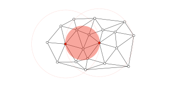
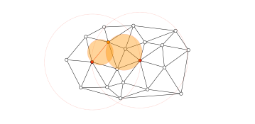
(a) (b) (c)

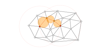
Figure 14: Finding a matching for two points given in red within a Delaunay triangulation. (a) Consider the circle centered at the midpoint between the points with diameter equal to their distance. Given the interior is non-empty, choose one of the interior points and iterate the process between the two original points and this midpoint. (b) The circle on the left contains no points, thus indicating the points must share an edge in the triangulation. The circle on the right is again non-empty, as such again break this problem into two and iterate. (c) Two further valid matching are found, completing the search for the overall path between the original vertices.

Before we discuss the main result of this section, we present a useful Lemma for a non-special system of points (that is one where the Delaunay triangulation is unique).

Lemma 18.

Given the graph $\mathcal{G}=(\mathcal{V},\mathcal{E})$ corresponding to the Delaunay triangulation of a non-special set of vertices $\mathcal{V}$ in $D$-dimensional space. Consider two vertices $A$ and $B$ such that there exists a hypersphere whose boundary contain $A$ and $B$ and whose interior contains no other vertices. Then, there must exist an edge $e\in\mathcal{E}$ between $A$ and $B$.

Proof.

If the hypersphere that contains $A$ and $B$ on its boundary with empty interior contains a further $D-1$ points on its boundary, then these $D+1$ points form a simplex in the Delaunay triangulation and all share edges, completing the proof. If the boundary contains fewer than that number of points, consider the continuous growth of all possible $D$-dimensional hyperpheres containing all points that are currently on the boundary, such a growth will be constrained to hyperspheres centered on a restricted hyperplane and can be made continuously until a large enough hypersphere is found that has $D+1$ vertices on its boundary. Such a hypersphere is guaranteed to exist due to the non-special nature of the vertex set and as such we have found the corresponding simplex that contains both $A$ and $B$, and thus shows they share an edge. ∎

Given the above Lemma, we are now ready to prove the main result of the section, which is a reformulation of the graph desiderata from Theorem 3 in the case of geometrically-local codes.

Theorem 19.

Given a (unique) Delaunay triangulation of an irreducible logical operator $\mathcal{L}$ of a geometrically-local code with stabilzer radius bounded by $R_{\mathcal{S}}$ the resulting graph $\mathcal{G}=(\mathcal{V},\mathcal{E})$ will have the following properties:

1. $\mathcal{G}$ is connected.

2. $\mathcal{G}$ vertex degree that is bounded by $O\left(((D+1)R_{\mathcal{S}})^{D}\right)$, that is a constant independent of system-size (yet dependent on dimension $D$).

3. For all local stabilizer generators of the code $S_{i}$ restricted to $\mathcal{L}$, the resulting matching of associated vertices in $\mathcal{G}$ is bounded, $|\mu(\mathcal{L}_{S_{i}})|=O(R_{\mathcal{S}}^{D})$. Each edge can belong to at most $O(R_{\mathcal{S}}^{2D})$ matchings.

4. There is a cycle basis of $G$ such that (a) each cycle is length $3$ and (b) each edge is involved in at most $O\left(((D+1)R_{\mathcal{S}})^{D}\right)$ cycles.

Proof.

By definition the Delaunay triangulation is connected, thus proving point 0.

Given we have a logical operator that has to preserve some local structure, there exists a radius $R_{\mathcal{L}}$ of constant size, such that any hypersphere whose radius is at least $R_{\mathcal{L}}$ must contain $D+1$ points in its interior (or boundary) due to the constant density of points in the logical operator, by definition. As such, any circum-hypersphere of a simplex in Delaunay triangulation must have radius upper-bounded by $R_{\mathcal{L}}=(D+1)R_{\mathcal{S}}$. As such, a given vertex may only share an edge with another vertex in the graph if they belong to the same circum-hypersphere, and as such must be within distance $2R_{\mathcal{L}}$ of one another. Therefore, the total number of neighbors a given vertex $v\in\mathcal{V}$ can have is bounded by the number of vertices within the hypersphere of radius $2R_{\mathcal{L}}$, centered at $v$, which is at most $\rho(2R_{\mathcal{L}})^{D}$ by the definition of a geometrically-local code, proving point 1.

We will return to the proof of point 2 below, yet the proof of point 3 is simple. Given the Delaunay triangulation forms a graph composed of simplicies, the faces of the graph are all triangles. Therefore, a valid cycle basis for the graph is the set of all triangular faces, which are all of length 3. Moreover, given each edge by definition is associated with a pair of points (its endpoints), in order for such an edge to be involved in a triangular face, the pair of endpoints must share a common neighbor in the graph. Since the number of neighbors for each individual endpoint is upper-bounded by $\rho(2R_{\mathcal{L}})^{D}$, their common neighbors must be similarly upper-bounded, thus proving point 3.

Finally, we arrive at the proof of point 2. Given a stabilizer $S_{i}$ that anti-commutes with the given logical operator at an even number of qubits, this will correspond to an even number of vertices in the graph $\mathcal{G}$. We are tasked with finding a matching for these vertices that is of bounded length. Given the stabilizer is local, the resulting set of vertices on the graph $\mathcal{G}$ are local, that is they are all within a hypersphere of constant radius $R_{\mathcal{S}}$. We can choose to match any two pairs of points, as we will show that we can find a path in $\mathcal{G}$ of bounded length (not necessarily minimum-matching). Given two points $A$ and $B$, consider the hypersphere $H_{AB}$ centered at the midpoint between these points, whose diameter is the distance between these points (thus $A$ and $B$ reside on the boundary of this hypersphere, and the diameter must be upper bounded by $R_{\mathcal{S}}$). If there are no points of $\mathcal{G}$ in the interior of $H_{AB}$ then $A$ and $B$ must belong to the same simplex in the Delauney triangulation (by Lemma 18) and as such we have found a path. If there does exist any points in the interior of $H_{AB}$, choose any such point and denote it $C$. Now, we can iterate the search for an edge with the new pairings: $AC$ and $BC$, thus breaking the original problem into two equivalent subproblems. Given $C$ is in the interior of $H_{AB}$, the geometric distance between $A$ and $C$ as well as $B$ and $C$ must be strictly less that $A$ and $B$. Given there are only a finite number of vertices within the hypersphere of constant radius $R_{\mathcal{S}}$, upper bounded by $\rho R_{\mathcal{S}}^{D}$, the search will terminate in a finite number of steps resulting in a path with at most $O(R_{\mathcal{S}}^{D})$ edges. Finally, we would like to bound the number of times a given edge is used in matchings of different stabilizer generators, restricted to $\mathcal{L}$. Given all edges in the matching of two points $A$ and $B$ must be withing the hyperspheres of radius $R_{\mathcal{S}}$ of each point, there can only be a finite number of pairings of points for which a given edge can belong. The number of such pairings of points would necessarily be upper-bounded by $O\left((R_{\mathcal{S}}^{D})^{2}\right)$. ∎

We have shown that we can create a graph satisfying desiderata (0-3) for any geometrically-local code. This is enough, say, for use of the toric code adapter from Sec. 5 on such codes without suffering a loss of code distance in the deformed code, since the toric code adapter does not require desiderata (4).

More generally, it is true that desiderata (4) is not necessary for using even the repetition code adapter of Sec. 4 on some geometrically-local codes. For instance, in some $D$-dimensional toric codes [57, 58, 59, 60], the logical $Z$-type operators $\overline{Z}_{0},\overline{Z}_{1},\dots,\overline{Z}_{D-1}$ are 1-dimensional and run in orthogonal directions through the lattice. This means that a gauging measurement of one of these cannot decrease the weight of another in the resulting deformed code. Exploring the extent to which we can avoid desiderata (4) in special cases we leave to future work.

7 Discussion

We found the notion of relative expansion defined in Definition 1 useful for our proofs of code distance and our graph constructions. It is also significantly weaker than requiring the graph have constant global expansion. However, in some cases, even relative expansion may be unnecessary. One simple example of this case is the fault-tolerant lattice surgery between two surface code patches, which is part of the gauging measurement framework [31] (and an example of CSS code surgery [28]), but the relative expansion of the auxiliary graph decreases with the code distance as $O(1/d)$. This seems to be sufficient partly because the surface code does not encode more than one logical qubit. Is there a way to more accurately capture the necessary expansion properties of the auxiliary graph in general?

There are some assumptions placed on the adapter of Section 4 that are likely not strictly necessary. We mentioned in that section the potential to attach adapters to separate ports and the potential for a notion of multi-port relative expansion. In addition, it would be nice to be able to measure the product of overlapping or reducible logical operators in general within the framework we have presented.

Decoding through the process of gauging measurement involves decoding the deformed code(s) created in the process. In Ref. [29], a modular decoder is introduced which can split this decoding problem (for one type of Pauli error) into two spatially separate pieces – an LDPC decoding problem on the original code, and a matching problem on the auxiliary graph. We expect the same modular decoding can be done for gauging measurement, but splitting the decoding problem further when measuring a large product of logical operators would seem to be necessary for fast decoding of LDPC surgery in practice, unless this situation can otherwise be avoided.

Our sparse basis transformation method by means of the $\mathsf{SkipTree}$ algorithm helped give rigorous guarantees on the deformed code to be LDPC. This enabled a host of joint-measurement schemes that allow one to implement logical Clifford gates fault-tolerantly on arbitrary LDPC codes. The sparse basis transformation also gave rise to a concrete hybrid lattice surgery and unitary scheme that allows one to implement logical gates available in other codes between logical qubits of our original LDPC code. Although this paper specifically discussed targeted $\overline{\mathsf{CNOT}}$ using Dehn twists on a toric code, we expect similar adaptors to be constructed that enable known gates from a richer variety of codes with similar distance to be connected to an efficient LDPC memory.

Appendix A Proofs for Theorem 3

A.1 Codespace of the deformed code in gauging measurement

Here we show that desideratum 0 in Theorem 3 is sufficient for the gauging measurement to measure the desired operator $\overline{Z}=Z(\mathcal{L})$. It is also necessary without loss of generality, as we remark below.

Lemma 20.

Provided $\mathcal{G}$ is connected, the deformed code in gauging measurement (see Fig. 3) has one less logical qubit than the original code and $\overline{Z}=Z(\mathcal{L})$ is in the stabilizer group of the deformed code.

Proof.

Let $\overline{X}_{i},\overline{Z}_{i}$ for $i=0,1,\dots,k-1$ denote a symplectic basis of logical operators for the original code. That is, $\overline{X}_{i}$ and $\overline{Z}_{j}$ anticommute if and only if $i=j$. Note these do not have to be $X$ and $Z$ type operators as we are considering an arbitrary (potentially non-CSS) stabilizer code. We let $\overline{Z}_{0}$ be the operator $\overline{Z}=Z(\mathcal{L})$ being measured.

We apply stabilizer update rules [40] to a basis of the normalizer of the original stabilizer group. Initially, this is the normalizer group of the original code as well as single qubit operators $\{X(e)\}_{e\in\mathcal{E}}$ on each edge qubit. We measure all stabilizers of the deformed code Fig. 3.

Suppose $\Lambda$ is one of the stabilizers of the original code or one of the logicals $\overline{X}_{i},\overline{Z}_{i}$ for $i=1,2,\dots,k-1$. These all commute with $\overline{Z}$. If the $X$-type support of $\Lambda$ on $\mathcal{L}$ is $\mathcal{L}_{\Lambda}$, then $|\mathcal{L}_{\Lambda}|$ is even, and $\Lambda$ anticommutes with an even number of checks in $\mathcal{V}$, exactly those on vertices $f(\mathcal{L}_{\Lambda})$. Find a perfect matching $\mu(\mathcal{L}_{\Lambda})$ of those vertices in the graph $G$ (which exists because $G$ is connected). We see we can update $\Lambda$ to commute with all $\mathcal{V}$ checks by multiplying by the appropriate combination of initial edge stabilizers $X(e)$, namely,

$$\Lambda\rightarrow\Lambda\prod_{e\in\mu(\mathcal{L}_{\Lambda})}X(e).$$ (55)

Thus, by updating $\overline{X}_{i},\overline{Z}_{i}$ for $i=1,2,\dots,k-1$ this way, there is a symplectic basis for $k-1$ logical qubits in the deformed code.

The original stabilizers $X(e)$ must be updated to form products $X(c\in\mathcal{E})$ that commute with all vertex checks $\mathcal{V}$. This necessitates they form cycles in the graph, i.e. $cG=0$. Therefore, the checks $\mathcal{U}$ capture a complete basis of these combinations.

Moreover, the product of all checks in $\mathcal{V}$, i.e. $\mathcal{H}_{Z}(\mathcal{V})$, equals $\overline{Z}=Z(\mathcal{L})$. This product of checks has no support on edge qubits $\mathcal{E}$ because $\vec{1}G^{\top}=0$. Thus, $\overline{Z}$ is in the stabilizer group of the deformed code. ∎

We remark that desiderata 0 is technically a little too strong to reach the conclusion of this lemma and thus for the claim in Theorem 3. All we really need is $f(\mathcal{L})$ to be a connected subset of vertices in $\mathcal{G}$, i.e. it is possible to get between any two vertices of $f(\mathcal{L})$ via a path in $\mathcal{G}$. However, this places $f(\mathcal{L})$ entirely within one connected component of $\mathcal{G}$ and other connected components can easily be shown to represent stabilizer states separable from the deformed code. Thus, we consider $\mathcal{G}$ to be connected without loss of generality.

A.2 Code distance of the deformed code in gauging measurement

Here we show that desideratum 4 of Theorem 3 is sufficient to guarantee the deformed code has good code distance.

Lemma 21.

Provided $\mathcal{G}$ and the port function $f$ are chosen such that $\beta_{d}(\mathcal{G},f(\mathcal{L}))\geq 1$ where $d$ is the code distance of the original code, the deformed code in gauging measurement (see Fig. 3) has code distance at least $d$.

Proof.

Similar proofs exist in [29, 31]. Our new contribution is to use relative expansion.

Consider an arbitrary non-trivial logical operator of the deformed code $\overline{L}=L_{X}L_{Z}$ where $L_{X}$ is an $X$-type Pauli and $L_{Z}$ a $Z$-type Pauli. Let $\overline{L}\equiv\overline{L}^{\prime}$ indicate the equivalence of $\overline{L}$ and $\overline{L}^{\prime}$ modulo the checks of the deformed code. We start by finding such an equivalent $\overline{L}^{\prime}$ with convenient qubit support. Then, we show that the weight of $\overline{L}^{\prime}$ cannot be reduced below $d$, the original code’s distance, by multiplying by any combination of the deformed code’s checks. Thus, the weight of $\overline{L}$ cannot be reduced in this way either.

Consider the restriction of $L_{Z}$ to the qubits $\mathcal{E}$, denoted $Z(u\in\mathcal{E})$. Because $\overline{L}$ commutes with all checks in $\mathcal{U}$, we must have $Nu^{\top}=0$. By construction of $N$, its row space equals the row nullspace of $G$. This also means the column nullspace of $N$ equals the column space of $G$. Thus, there exists $v$ such that $u^{\top}=Gv^{\top}$ and $u=vG^{\top}$. As a result, $L_{Z}$ can be cleaned from $\mathcal{E}$ by multiplying by appropriate checks from $\mathcal{V}$. Explicitly,

$$\overline{L}\equiv\overline{L}^{\prime}=\overline{L}\mathcal{H}_{Z}(v\in\mathcal{V}),$$ (56)

and $\overline{L}^{\prime}$ has no $Z$-type support on $\mathcal{E}$.

Now the restriction of $\overline{L}^{\prime}$ to the qubits of the original code must commute with all checks of the original code and is therefore a logical operator $\overline{\Lambda}$ of the original code. That is,

$$\overline{L}^{\prime}=\overline{\Lambda}X(c\in\mathcal{E}),$$ (57)

for some vector $c$.

Suppose $\overline{\Lambda}$ is a trivial logical operator of the original code, i.e. a product of original code checks. Then, multiplying by those checks to remove it from the original code, we obtain

$$\overline{L}^{\prime}\equiv X(c^{\prime}\in\mathcal{E}).$$ (58)

Of course, this operator must commute with all vertex $Z$ checks $\mathcal{V}$, so $cG=0$. This implies $\overline{L}^{\prime}$ is a cycle in the graph, so it will be a product of the checks $\mathcal{U}$. This is a contradiction with our assumption that $\overline{L}$ is a nontrivial logical operator of the deformed code.

Therefore, $\overline{\Lambda}$ is a nontrivial logical operator of the original code, and the weight of $\overline{L}^{\prime}=\overline{\Lambda}X(c\in\mathcal{E})$ is at least $d$ even if the $X$-type support on $\mathcal{E}$ is ignored. To show $\overline{L}^{\prime}$ cannot be reduced in weight by multiplying by checks from $\mathcal{V}$, we show that $\overline{\Lambda}$ cannot be reduced in weight this way.

Suppose $\overline{\Lambda}=\Lambda_{X}\Lambda_{Z}$ and consider $|\overline{\Lambda}\mathcal{H}_{X}(v\in\mathcal{V})|$ for any choice of vector $v$ indicating a set of vertices $\mathcal{V}$. We define the sets of qubits $\mathcal{L}^{*}:=\mathcal{L}\setminus\operatorname{supp}{\Lambda_{X}}$ and $\mathcal{R}:=\operatorname{supp}{\overline{\Lambda}}\setminus\mathcal{L}^{*}$. We also let $w$ be the restriction of $v$ to the vertices $f(\mathcal{L}^{*})\subseteq\mathcal{V}$. Thus, $\mathcal{W}:=f^{-1}(\operatorname{supp}{w})$ is a subset of qubits in $\mathcal{L}^{*}$. The intersection profile of $\mathcal{L}^{*}$, $\mathcal{W}$, and $\operatorname{supp}{\Lambda_{Z}}$ defines four subsets $\alpha,\beta,\gamma,\delta\subseteq\mathcal{L}^{*}$. These sets are illustrated in Fig. 15. From the figure, it is clear that

$$d \leq|\overline{\Lambda}|=|\gamma|+|\delta|+|\mathcal{R}|,$$ (59)

$$d \leq|\overline{\Lambda}\;\overline{Z}|=|\alpha|+|\beta|+|\mathcal{R}|.$$ (60)

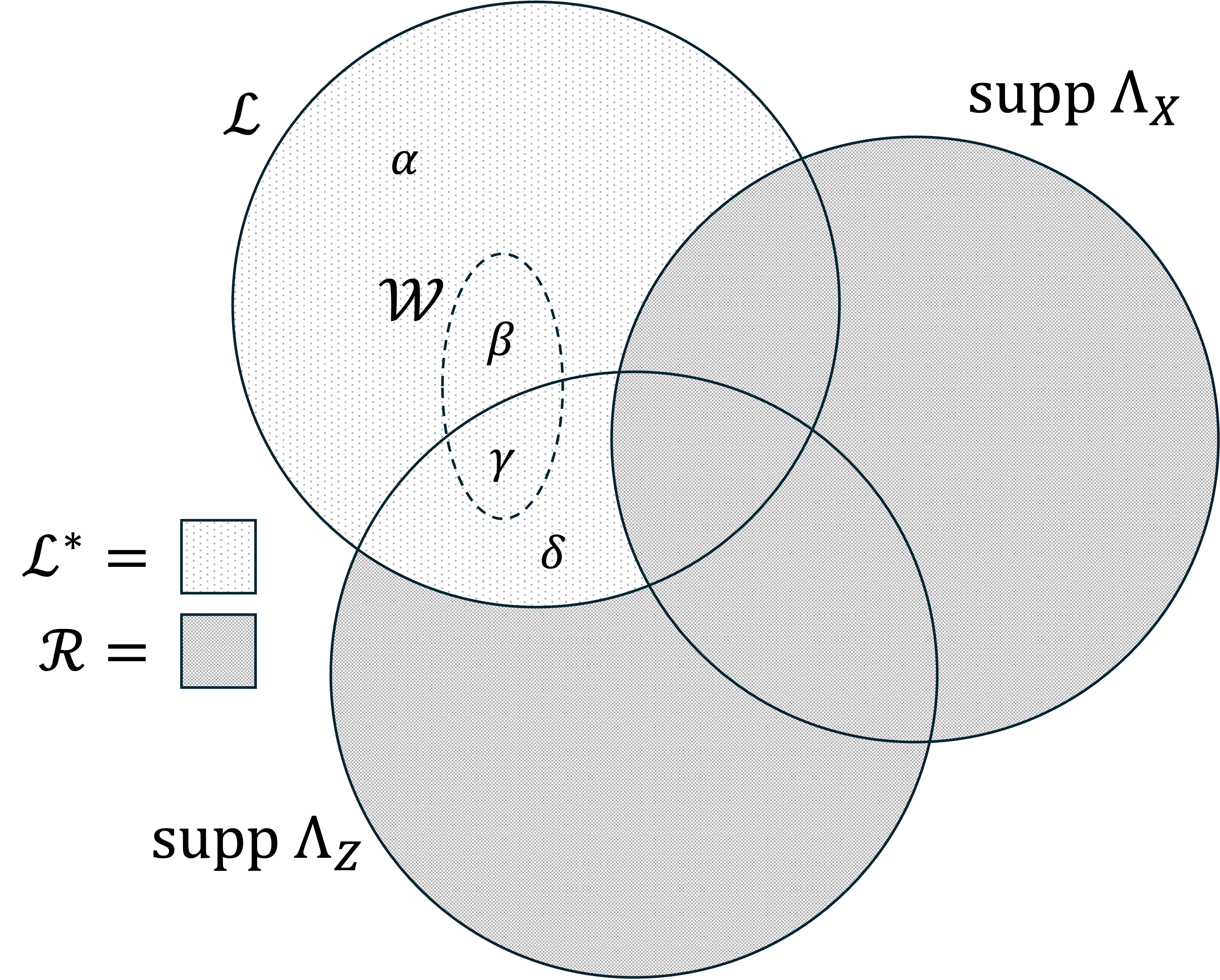
Figure 15: A summary of the qubit sets used in the final part of the proof of Lemma 21, the deformed code distance in gauging measurement. These are all subsets of the qubits of the original code. Here $\mathcal{L}$ supports the logical operator $\overline{Z}=Z(\mathcal{L})$ being measured. Another logical operator $\overline{\Lambda}=\Lambda_{X}\Lambda_{Z}$ generally intersects $\overline{Z}$. The dashed region within $\mathcal{L}^{*}$ represents $\mathcal{W}$, which defines the four subregions $\alpha,\beta,\gamma,\delta\subseteq\mathcal{L}^{*}$.

By assumption the relative expansion $\beta_{d}(\mathcal{G},f(\mathcal{L}))$ is at least $1$. Because $f(\mathcal{L^{*}})\subseteq f(\mathcal{L})$, Lemma 2 implies $\beta_{d}(\mathcal{G},f(\mathcal{L^{*}}))\geq\beta_{d}(\mathcal{G},f(\mathcal{L}))\geq 1$.

We now calculate

$$|\overline{\Lambda}\mathcal{H}_{Z}(v\in\mathcal{V})| =|\beta|+|\delta|+|\mathcal{R}|+|vG^{\top}|$$ (61)

$$\geq|\beta|+|\delta|+|\mathcal{R}|+\min(d,|w|,|\mathcal{L}^{*}|-|w|)$$ (62)

$$=|\beta|+|\delta|+|\mathcal{R}|+\min(d,|\mathcal{W}|,|\mathcal{L}^{*}|-|\mathcal{W}|)$$ (63)

$$=|\beta|+|\delta|+|\mathcal{R}|+\min(d,|\beta|+|\gamma|,|\alpha|+|\delta|),$$ (64)

where the inequality makes use of relative expansion on $f(\mathcal{L}^{*})$. If the minimum evaluates to $d$, then it is immediate that $|\overline{\Lambda}\mathcal{H}_{Z}(v\in\mathcal{V})|\geq d$. If the minimum evaluates to $|\beta|+|\gamma|$, use Eq. (59) to conclude $|\overline{\Lambda}\mathcal{H}_{Z}(v\in\mathcal{V})|\geq d$. If the minimum evaluates to $|\alpha|+|\delta|$, use Eq. (60) to conclude similarly. ∎

Appendix B Support lemma for irreducible logical operators

Here we record a helpful support lemma from Ref. [29], there Lemma 8.

Lemma 22.

[29] Let $H=[H_{X}|H_{Z}]$ be the (symplectic) parity check matrix of an $n$-qubit stabilizer code, $\overline{Z}$ be an irreducible logical $Z$-type operator, and $H^{\prime}_{X}$ denote the sub-matrix of $H_{X}$ restricted to qubits in the support of $\overline{Z}$. Then, $H^{\prime}_{X}v^{\top}=0$ implies $v=0$ or $v=\vec{1}$. Equivalently, $H^{\prime}_{X}$ is a check matrix of the classical repetition code.

Proof.

If $v$ is not $0$ or $\vec{1}$, then it implies a logical $Z$-type operator $Z(v)$ of the stabilizer code exists that is entirely supported within the support of $\overline{Z}$. This contradicts the definition of $\overline{Z}$ being irreducible. ∎

This lemma has a simple corollary.

Corollary 23.

If $\overline{Z}$ is an irreducible $Z$-type logical operator of a stabilizer code, and $P_{X}$ is an $X$-type operator (not necessarily logical) commuting with $\overline{Z}$, then there is a stabilizer $S$ of the code such that $SP_{X}$ does not have $X$-type support overlapping $\overline{Z}$. If the code is CSS, then $S$ can be chosen to be $X$-type and $SP_{X}$ does not overlap $\overline{Z}$ at all.

Proof.

Because it commutes with $\overline{Z}$, $P_{X}$ must overlap $\overline{Z}$ on an even number of qubits. Lemma 22 implies the $X$ check matrix of the code restricted to $\operatorname{supp}{\overline{Z}}$ generates all even weight $X$ operators. Thus, we can find a stabilizer $S$ performing as claimed. ∎

Appendix C $\mathsf{SkipTree}$ for the full-rank check matrix of the repetition code

We present a $\mathsf{SkipTree}$ algorithm variant specifically for solving $TGP=H_{R}$ for sparse matrix $T$ and permutation matrix $P$. The need for this is illustrated by a simple example. If $G=H_{R}$ is the incidence matrix of the path graph, applying Algorithm 1 creates a $(2,2)$-sparse matrix $T$. Clearly, however, the sparsest possible $T$ matrix is $(1,1)$-sparse, i.e. $T=P=I$.

Because Algorithm 1 is built to solve $TGP=H_{C}$ it always leaves some nodes unlabeled as it moves down the tree so that it can eventually find a way back to the root. Instead, when solving $TGP=H_{R}$ returning to the root is unnecessary, and only some branches of the spanning tree must be explored via the “skipping” behavior of Algorithm 1. This motivates the addition of a flag, $\mathsf{skip}\in\{\mathsf{True},\mathsf{False}\}$, that can toggle the skipping behavior on and off. Adding this, we obtain Algorithm 2 that produces sparser solutions for $T$. For example, it solves the case of the path graph optimally.

Algorithm 2 Given a connected graph $G\in\mathbb{F}_{2}^{\;m\times n}$, find $T\in\mathbb{F}_{2}^{\;n-1\times m}$ and permutation matrix $P\in\mathbb{F}_{2}^{\;n\times n}$ such that $TGP=H_{R}$. Both $T$ and $P$ have just $O(n)$ nonzero entries and could be constructed and returned as sparse matrices.

1:procedure $\mathsf{SkipTreeHR}$($G$)

2:     $S\leftarrow$ a spanning tree of $G$ $\triangleright$ has incidence matrix $S_{I}\in\mathbb{F}_{2}^{\;n-1\times n}$ that we do not need to store

3:     Index $\leftarrow 0$

4:     $\mathrm{Label}\leftarrow$ empty list of length $n$

5:     procedure $\mathsf{LabelFirst}$($v$,$\;\mathsf{skip}$)

6:         $\mathrm{Label}[\mathrm{Index}]\leftarrow v$

7:         Index $\leftarrow$ Index + 1

8:         for each child of vertex $v$ in $S$ do $\triangleright$ Recall the youngest child is the last in the for-loop.

9:              if child is youngest and $\mathsf{skip}=\mathsf{False}$ then

10:                  $\mathsf{LabelFirst}(\mathrm{child},\mathsf{skip}=\mathsf{False})$

11:              else

12:                  $\mathsf{LabelLast}(\mathrm{child})$                             

13:     procedure $\mathsf{LabelLast}$($v$)

14:         for each child of vertex $v$ in $S$ do

15:              $\mathsf{LabelFirst}(\mathrm{child},\mathsf{skip}=\mathsf{True})$          

16:         $\mathrm{Label}[\mathrm{Index}]\leftarrow v$

17:         Index $\leftarrow$ Index + 1      

18:     $\mathsf{LabelFirst}(0,\mathsf{skip}=\mathsf{False})$ $\triangleright$ Root is 0. After this line, $\mathrm{Label}[l]=v$ means vertex $v$ is labeled $l$.

19:     $P\leftarrow n\times n$ matrix with $P_{vl}=1$ iff $\mathrm{Label}[l]=v$.

20:     $\tilde{T}\leftarrow$ matrix with $n-1$ rows and $n-1$ columns.

21:     $\tilde{T}_{le}=1$ iff edge $e$ is part of the shortest path in $S$ from $\mathrm{Label}[l]$ to $\mathrm{Label}[l+1]$. $\triangleright$ now $\tilde{T}S_{I}=H_{R}P^{\top}$

22:     Add zero columns to $\tilde{T}$, obtaining $T$ so that $TG=\tilde{T}S_{I}$.

23:     Return $T$, $P$.

Appendix D Proofs on the Toric Code adapter

D.1 Proof that $\mathcal{G}_{\textrm{merge}}$ has $k$ logical qubits

See 13

Proof.

Let the qubits in the remainder of the original LDPC code (i.e. the complement of qubit sets $\mathcal{L}^{Z}$ and $\mathcal{L}^{X}$, supporting logicals $\bar{Z}_{c}$ and $\bar{X}_{t}$, each corresponding to a different logical qubit) be labelled by $\mathcal{R}$. Note that irreducible logicals $\bar{Z}_{c}$ and $\bar{X}_{t}$ can be assumed to be disjoint without loss of generality, as any overlapping support between the two can be cleaned by stabilizer multiplication (see corollary 23 for proof).

We can partition the check matrix $H_{X}$ into three blocks: the support of the original code $X$-checks which overlap the specific $\bar{Z}_{c}$ logical, $H_{X}|_{\operatorname{supp}{(\bar{Z}_{c})}}$ described by a matrix $A_{Z}$, $H_{X}|_{\operatorname{supp}{(\bar{X}_{t})}}$ by a binary matrix $C_{Z}$ and support on the remaining physical qubits $\mathcal{R}$ by $B_{Z}$. The check matrix of the base code for relevant $X$ checks (ie. $X$ checks which overlap $\bar{Z}_{c}$) is given by $H_{X}=\begin{bmatrix}B_{Z}&A_{Z}&C_{Z}\end{bmatrix}$.

The ancilla system consists of three - qubits belonging to set $\mathcal{E}^{Z}$ initialized in single-qubit $\ket{+}$ states, qubits belonging to set $\mathcal{E}^{X}$ initialized in single-qubit $\ket{0}$ states and the toric code ancilla state. $\mathcal{G}_{\mathrm{aux}}^{Z}\cup\mathcal{G}_{\mathrm{toric}}\cup\mathcal{G}_{\mathrm{aux}}^{Z}$. Qubits initialized in single qubit $\ket{+}$ or $\ket{0}$ states, which is equivalent to adding single-qubit $X$ and $Z$ checks to the code. Qubits in sets $\mathcal{Q}^{Z}_{0}$ are initialized with single qubit $X$ stabilizers, and qubits in sets $\mathcal{Q}^{X}_{0}$ are initialized with single qubit $Z$ stabilizers. The toric code ancilla is initialized in a specific eigenstate of the toric code - namely the simultaneous $+1$ eigenspace of the logicals $\bar{Z}_{2}$ and $\bar{X}_{1}$.

The number of physical qubits $n^{\prime}$ in the system, including the physical qubits from the base code and ancilla qubits

$$n^{\prime} =n+|\mathcal{E}^{X}|+|\mathcal{E}^{Z}|+d|\mathcal{Q}^{X}_{0}|+d|\mathcal{Q}^{Z}_{0}|$$

$$=n+|\mathcal{E}^{X}|+|\mathcal{E}^{Z}|+d|\mathcal{V}^{X}|+d|\mathcal{V}^{Z}|$$ (65)

Here we use the fact that there is a one-to-one correspondence between physical qubits introduced and the new checks in $\mathcal{V}^{X}$ and $\mathcal{V}^{Z}$, up to a permutation.

It is trivially true that the single qubit stabilizers are linearly independent of one another, due to their distinct qubit support. Further since the count of these stabilizers is exactly equal to the count of ancilla qubits, they do not add any logical qubits to the code.

Next, we deform the code by measuring stabilizers of the new code. In every layer, a $X$-check is introduced for each qubit in the support of $\bar{X}_{t}$, which means the number of $X$ checks in each layer, $|\mathcal{C}^{X}_{i}|=|\mathcal{L}^{X}|(=d)$ for $i=0,...,d-1$. Since there is a one-to-one correspondence between qubits in $\mathcal{L}^{X}$ and qubits in $\mathcal{V}^{X}$ by injective map $f$ (set up in section 2.3), we have $|\mathcal{C}^{X}_{i}|=|\mathcal{L}^{X}|=|\mathcal{V}^{X}|$.

The desired new code after code deformation has $X$-checks given by

$$H_{X}^{\prime} =\bordermatrix{&\mathcal{R}&\mathcal{L}^{Z}&\mathcal{L}^{X}&\mathcal{E}^{Z}&\mathcal{Q}^{Z}_{0}&\mathcal{Q}^{X}_{0}&\mathcal{Q}^{Z}_{1}&\mathcal{Q}^{X}_{1}&...&\mathcal{Q}^{X}_{d-2}&\mathcal{Q}^{Z}_{d-1}&\mathcal{Q}^{X}_{d-1}&\mathcal{E}^{X}\cr\mathcal{B}^{X}&B_{Z}&A_{Z}&C_{Z}&M_{Z}&&&&\cr\mathcal{U}^{Z}&&&&N_{Z}&&&&\cr\mathcal{C}^{X}_{0}&&&&T_{Z}&H_{C}&I&&&&&&I\cr\mathcal{C}^{X}_{1}&&&&&&I&H_{C}&I&&&&&\cr\vdots&&&&&&&&&\ddots&&&\cr\mathcal{C}^{X}_{d-1}&&&&&&&&&&I&H_{C}&I\cr\mathcal{V}^{X}&&&I&&&&&&&&&P_{X}&G_{X}^{\intercal}\cr}\qquad$$ (66)

Perform row operation $\mathcal{C}^{X}_{0}\rightarrow\mathcal{C}^{X}_{0}+\sum_{i=1}^{d-1}\mathcal{C}^{X}_{i}$.

$$\rightarrow \qquad\bordermatrix{&\mathcal{R}&\mathcal{L}^{Z}&\mathcal{L}^{X}&\mathcal{E}^{Z}&\mathcal{Q}^{Z}_{0}&\mathcal{Q}^{X}_{0}&\mathcal{Q}^{Z}_{1}&\mathcal{Q}^{X}_{1}&...&\mathcal{Q}^{X}_{d-2}&\mathcal{Q}^{Z}_{d-1}&\mathcal{Q}^{X}_{d-1}&\mathcal{E}^{X}\cr\mathcal{B}^{X}&B_{Z}&A_{Z}&C_{Z}&M_{Z}&&&&\cr\mathcal{U}^{Z}&&&&N_{Z}&&&&\cr\mathcal{C}^{X}_{0}&&&&T_{Z}&H_{C}&0&H_{C}&0&&0&H_{C}&0\cr\mathcal{C}^{X}_{1}&&&&&&I&H_{C}&I&&&&&\cr\vdots&&&&&&&&&\ddots&&&\cr\mathcal{C}^{X}_{d-1}&&&&&&&&&&I&H_{C}&I\cr\mathcal{V}^{X}&&&I&&&&&&&&&P_{X}&G_{X}^{\intercal}\cr}\qquad$$ (67)

In order to calculate the rank of $H_{X}^{\prime}$, we will consider the ranks of submatrices consisting of sets of rows, where it is clear that no row from one set can be expressed as a linear combination of rows from another set.

First, consider the sets of checks labelled by $\mathcal{B}^{X}$. The rank is the same as the rank of the original check matrix $H_{X}$. Next, consider the checks from the gauge-fixing set $\mathcal{U}^{Z}$. We will use the fact that the dimension of any cycle basis of any graph with $E$ edges, $V$ vertices and $c$ connected components is given by its cyclomatic number, $|E|-|V|+c$. Recall the $X$ checks in $\mathcal{U}^{Z}$ are added to deal with redundancies due cycles present in the new $Z$ checks. Each $X$ check corresponds to a cycle in the graph given by edges (qubits) in $\mathcal{E}^{Z}$ and vertices in $\mathcal{V}^{Z}$. Since there is only one connected component ($c=1$), $\mathrm{rank}(N_{Z})=|\mathcal{E}^{Z}|-|\mathcal{V}^{Z}|+1$.

Next, we consider the check matrix rows corresponding to $\mathcal{C}^{X}_{0}$ checks. The check matrix rows of $\mathcal{C}^{X}_{0}$ now only consists of $T_{Z}$ and $H_{C}$ as submatrices. These will determine $\mathrm{rank}(\mathcal{C}^{X}_{0})$, where $\mathrm{rank}(\mathcal{C}^{X}_{0})=\max(\mathrm{rank}(T_{Z}),\mathrm{rank}(H_{C}))$, as the rank of a matrix is equal to the number of rows of the largest square submatrix that has a nonzero determinant. We know $T_{Z}$ is a $|\mathcal{V}^{Z}|\times|\mathcal{E}^{Z}|$ matrix, and further, that one of the rows of $T_{Z}$ is redundant because the $\mathsf{SkipTree}$ algorithm returns to the original root vertex. We know the rank of $H_{C}$ is also $|\mathcal{V}^{Z}|-1$, since it has $d_{Z}=|\mathcal{V}^{Z}|$ rows in total, with one of the checks redundant.

Next, consider the checks corresponding to sets $\mathcal{C}^{X}_{i}$ for $1\leq i\leq d$. These rows are all identical modulo a cyclic shift, as they each have support $I$ on $\mathcal{Q}^{X}_{i-1}$ from the previous layer, $I$ on $\mathcal{Q}^{X}_{i}$ and $H_{C}$ on $\mathcal{Q}^{Z}_{i}$ within the same layer. Notice these rows are linearly independent of each other, for which it is sufficient to observe that their qubit support remains distinct even after row-column operations. The rank of the submatrix consisting of these rows is then the sum of the ranks of the individual sets of rows. Thus we obtain $\sum_{i=1}^{d-1}\mathrm{rank}(\mathcal{C}^{X}_{i})=(d-1)|\mathcal{V}^{X}|$.

$$\mathrm{rank}(H_{X}^{\prime}) =\mathrm{rank}(\mathcal{B}^{X})+\mathrm{rank}(N_{Z})+\mathrm{rank}(H_{C})+\sum_{i=1}^{d-1}\mathrm{rank}(\mathcal{C}^{X}_{i})+\mathrm{rank}(\mathcal{V}^{X})$$

$$=\mathrm{rank}(\mathcal{B}^{X})+(|\mathcal{E}^{Z}|-|\mathcal{V}^{Z}|+1)+(|\mathcal{V}^{Z}|-1)+(d-1)|\mathcal{V}^{X}|+|\mathcal{V}^{X}|$$

$$=\mathrm{rank}(H_{X})+|\mathcal{E}^{Z}|+d|\mathcal{V}^{X}|$$ (68)

Similarly,

$$\mathrm{rank}(H_{Z}^{\prime})=\mathrm{rank}(H_{Z})+|\mathcal{E}^{X}|+d|\mathcal{V}^{Z}|$$ (69)

The number of logical qubits $k^{\prime}$ in the deformed code

$$k^{\prime} =n^{\prime}-\mathrm{rank}(H_{X}^{\prime})-\mathrm{rank}(H_{Z}^{\prime})$$

$$=(n+|\mathcal{E}^{X}|+|\mathcal{E}^{Z}|+d|\mathcal{V}^{X}|+d|\mathcal{V}^{Z}|)-\mathrm{rank}(H_{X}^{\prime})-\mathrm{rank}(H_{Z}^{\prime})$$

$$=n-\mathrm{rank}(H_{X})-\mathrm{rank}(H_{Z})+|\mathcal{E}^{X}|+|\mathcal{E}^{Z}|+d|\mathcal{V}^{X}|+d|\mathcal{V}^{Z}|-|\mathcal{E}^{X}|-d|\mathcal{V}^{Z}|-|\mathcal{E}^{X}|-d|\mathcal{V}^{Z}|$$

$$=k$$ (70)

∎

References

- [1] Christian Kraglund Andersen, Ants Remm, Stefania Lazar, Sebastian Krinner, Nathan Lacroix, Graham J Norris, Mihai Gabureac, Christopher Eichler, and Andreas Wallraff. Repeated quantum error detection in a surface code. Nature Physics, 16(8):875–880, 2020.
- [2] Google Quantum AI. Exponential suppression of bit or phase errors with cyclic error correction. Nature, 595(7867):383–387, 2021.
- [3] Ciaran Ryan-Anderson, Justin G Bohnet, Kenny Lee, Daniel Gresh, Aaron Hankin, JP Gaebler, David Francois, Alexander Chernoguzov, Dominic Lucchetti, Natalie C Brown, et al. Realization of real-time fault-tolerant quantum error correction. Physical Review X, 11(4):041058, 2021.
- [4] J Ferreira Marques, BM Varbanov, MS Moreira, Hany Ali, Nandini Muthusubramanian, Christos Zachariadis, Francesco Battistel, Marc Beekman, Nadia Haider, Wouter Vlothuizen, et al. Logical-qubit operations in an error-detecting surface code. Nature Physics, 18(1):80–86, 2022.
- [5] Neereja Sundaresan, Theodore J Yoder, Youngseok Kim, Muyuan Li, Edward H Chen, Grace Harper, Ted Thorbeck, Andrew W Cross, Antonio D Córcoles, and Maika Takita. Demonstrating multi-round subsystem quantum error correction using matching and maximum likelihood decoders. Nature Communications, 14(1):2852, 2023.
- [6] Rajeev Acharya, Laleh Aghababaie-Beni, Igor Aleiner, Trond I Andersen, Markus Ansmann, Frank Arute, Kunal Arya, Abraham Asfaw, Nikita Astrakhantsev, Juan Atalaya, et al. Quantum error correction below the surface code threshold. arXiv preprint arXiv:2408.13687, 2024.
- [7] Dolev Bluvstein, Simon J Evered, Alexandra A Geim, Sophie H Li, Hengyun Zhou, Tom Manovitz, Sepehr Ebadi, Madelyn Cain, Marcin Kalinowski, Dominik Hangleiter, et al. Logical quantum processor based on reconfigurable atom arrays. Nature, 626(7997):58–65, 2024.
- [8] Jean-Pierre Tillich and Gilles Zémor. Quantum ldpc codes with positive rate and minimum distance proportional to the square root of the blocklength. IEEE Transactions on Information Theory, 60(2):1193–1202, 2013.
- [9] Alexey A. Kovalev and Leonid P. Pryadko. Fault tolerance of quantum low-density parity check codes with sublinear distance scaling. Phys. Rev. A, 87:020304, Feb 2013.
- [10] Anthony Leverrier, Jean-Pierre Tillich, and Gilles Zémor. Quantum expander codes. In 2015 IEEE 56th Annual Symposium on Foundations of Computer Science, pages 810–824. IEEE, 2015.
- [11] Omar Fawzi, Antoine Grospellier, and Anthony Leverrier. Constant overhead quantum fault tolerance with quantum expander codes. Communications of the ACM, 64(1):106–114, 2020.
- [12] Dominic J Williamson and Nouédyn Baspin. Layer codes. arXiv preprint arXiv:2309.16503, 2023.
- [13] Hayata Yamasaki and Masato Koashi. Time-efficient constant-space-overhead fault-tolerant quantum computation. Nature Physics, 20(2):247–253, 2024.
- [14] Nikolas P Breuckmann and Jens N Eberhardt. Balanced product quantum codes. IEEE Transactions on Information Theory, 67(10):6653–6674, 2021.
- [15] Pavel Panteleev and Gleb Kalachev. Asymptotically good quantum and locally testable classical ldpc codes. In Proceedings of the 54th Annual ACM SIGACT Symposium on Theory of Computing, pages 375–388, 2022.
- [16] Anthony Leverrier and Gilles Zémor. Quantum tanner codes. In 2022 IEEE 63rd Annual Symposium on Foundations of Computer Science (FOCS), pages 872–883. IEEE, 2022.
- [17] Daniel Gottesman and Isaac L Chuang. Demonstrating the viability of universal quantum computation using teleportation and single-qubit operations. Nature, 402(6760):390–393, 1999.
- [18] Peter W Shor. Proceedings of 37th conference on foundations of computer science, 1996.
- [19] David P DiVincenzo and Peter W Shor. Fault-tolerant error correction with efficient quantum codes. Physical review letters, 77(15):3260, 1996.
- [20] Andrew M Steane. Active stabilization, quantum computation, and quantum state synthesis. Physical Review Letters, 78(11):2252, 1997.
- [21] Emanuel Knill. Quantum computing with realistically noisy devices. Nature, 434(7029):39–44, 2005.
- [22] Dominic Horsman, Austin G Fowler, Simon Devitt, and Rodney Van Meter. Surface code quantum computing by lattice surgery. New Journal of Physics, 14(12):123011, 2012.
- [23] Daniel Litinski. A game of surface codes: Large-scale quantum computing with lattice surgery. Quantum, 3:128, March 2019.
- [24] Matthew B Hastings. Weight reduction for quantum codes. arXiv preprint arXiv:1611.03790, 2016.
- [25] Matthew B Hastings. On quantum weight reduction. arXiv preprint arXiv:2102.10030, 2021.
- [26] Eric Sabo, Lane G Gunderman, Benjamin Ide, Michael Vasmer, and Guillaume Dauphinais. Weight reduced stabilizer codes with lower overhead. arXiv preprint arXiv:2402.05228, 2024.
- [27] Lawrence Z. Cohen, Isaac H. Kim, Stephen D. Bartlett, and Benjamin J. Brown. Low-overhead fault-tolerant quantum computing using long-range connectivity. Science Advances, 8(20), may 2022.
- [28] Alexander Cowtan and Simon Burton. CSS code surgery as a universal construction. Quantum, 8:1344, 2024.
- [29] Andrew Cross, Zhiyang He, Patrick Rall, and Theodore Yoder. Linear-size ancilla systems for logical measurements in qldpc codes. arXiv preprint arXiv:2407.18393, 2024.
- [30] Alexander Cowtan. Ssip: automated surgery with quantum ldpc codes, 2024.
- [31] Dominic J. Williamson and Theodore J. Yoder. Low-overhead fault-tolerant quantum computation by gauging logical operators. arXiv preprint arXiv:2410.02213, 2024.
- [32] Benjamin Ide, Manoj G. Gowda, Priya J. Nadkarni, and Guillaume Dauphinais. Fault-tolerant logical measurements via homological measurement. arXiv preprint arXiv:2410.02753, 2024.
- [33] S. Bravyi, G. Smith, and J. A. Smolin. Trading classical and quantum computational resources. Physical Review X, 6(2), June 2016.
- [34] Robert Koenig, Greg Kuperberg, and Ben W. Reichardt. Quantum computation with turaev–viro codes. Annals of Physics, 325(12):2707–2749, December 2010.
- [35] Nikolas P Breuckmann, Christophe Vuillot, Earl Campbell, Anirudh Krishna, and Barbara M Terhal. Hyperbolic and semi-hyperbolic surface codes for quantum storage. Quantum Science and Technology, 2(3):035007, August 2017.
- [36] Ali Lavasani, Guanyu Zhu, and Maissam Barkeshli. Universal logical gates with constant overhead: instantaneous dehn twists for hyperbolic quantum codes. Quantum, page 180, 2019.
- [37] Michael Freedman and Matthew B. Hastings. Building manifolds from quantum codes, 2021.
- [38] Boris Delaunay. Sur la sphère vide. A la mémoire de Georges Voronoï. Bulletin de l’Académie des Sciences de l’URSS, Classe des Sciences Mathématiques et Naturelles, 8:793, 1934.
- [39] Qian Xu, J. Pablo Bonilla Ataides, Christopher A. Pattison, Nithin Raveendran, Dolev Bluvstein, Jonathan Wurtz, Bane Vasic, Mikhail D. Lukin, Liang Jiang, and Hengyun Zhou. Constant-overhead fault-tolerant quantum computation with reconfigurable atom arrays, 2023.
- [40] Daniel Gottesman. Stabilizer Codes and Quantum Error Correction. PhD thesis, Caltech, 1997.
- [41] A Robert Calderbank and Peter W Shor. Good quantum error-correcting codes exist. Physical Review A, 54(2):1098, 1996.
- [42] Andrew M steane. Error correcting codes in quantum theory. Physical Review Letters, 77(5):793, 1996.
- [43] A Yu Kitaev. Fault-tolerant quantum computation by anyons. Annals of physics, 303(1):2–30, 2003.
- [44] Claude Berge. The theory of graphs. Courier Corporation, 2001.
- [45] Jonathan L. Gross and Jay Yellen. Graph Theory and Its Applications (2nd ed.), chapter 4.6 Graphs and Vector Spaces, page pp. 197–207. CRC Press, 2005.
- [46] Bojan Mohar. Isoperimetric numbers of graphs. Journal of combinatorial theory, Series B, 47(3):274–291, 1989.
- [47] Gert Sabidussi. Graph multiplication. Mathematische Zeitschrift, 72(1):446–457, 1959.
- [48] Vladim G Vizing. The cartesian product of graphs. Vycisl. Sistemy, 9(30-43):33, 1963.
- [49] Michael E Beverland, Shilin Huang, and Vadym Kliuchnikov. Fault tolerance of stabilizer channels. arXiv preprint arXiv:2401.12017, 2024.
- [50] Thomas H Cormen, Charles E Leiserson, Ronald L Rivest, and Clifford Stein. Introduction to algorithms. MIT press, 2022.
- [51] Sergey Bravyi, Graeme Smith, and John A. Smolin. Trading classical and quantum computational resources. Physical Review X, 6(2), June 2016.
- [52] Theodore J. Yoder, Ryuji Takagi, and Isaac L. Chuang. Universal fault-tolerant gates on concatenated stabilizer codes. Physical Review X, 6(3), September 2016.
- [53] Mark A Webster, Armanda O Quintavalle, and Stephen D Bartlett. Transversal diagonal logical operators for stabiliser codes. New Journal of Physics, 25(10):103018, October 2023.
- [54] Daniel Gottesman. Fault-tolerant quantum computation with constant overhead. Quantum Info. Comput., 14(15–16):1338–1372, nov 2014.
- [55] Shilin Huang, Tomas Jochym-O’Connor, and Theodore J. Yoder. Homomorphic logical measurements. PRX Quantum, 4:030301, Jul 2023.
- [56] Scott Aaronson and Daniel Gottesman. Improved simulation of stabilizer circuits. Phys. Rev. A, 70:052328, Nov 2004.
- [57] Eric Dennis, Alexei Kitaev, Andrew Landahl, and John Preskill. Topological quantum memory. Journal of Mathematical Physics, 43(9):4452–4505, 2002.
- [58] Hector Bombin and Miguel A Martin-Delgado. Homological error correction: Classical and quantum codes. Journal of mathematical physics, 48(5), 2007.
- [59] Michael Vasmer and Dan E Browne. Three-dimensional surface codes: Transversal gates and fault-tolerant architectures. Physical Review A, 100(1):012312, 2019.
- [60] Tomas Jochym-O’Connor and Theodore J Yoder. Four-dimensional toric code with non-clifford transversal gates. Physical Review Research, 3(1):013118, 2021.