Not All Diffusion Model Activations
Have Been Evaluated as Discriminative Features

Abstract

Diffusion models are initially designed for image generation. Recent research shows that the internal signals within their backbones, named activations, can also serve as dense features for various discriminative tasks such as semantic segmentation. Given numerous activations, selecting a small yet effective subset poses a fundamental problem. To this end, the early study of this field performs a large-scale quantitative comparison of the discriminative ability of the activations. However, we find that many potential activations have not been evaluated, such as the queries and keys used to compute attention scores. Moreover, recent advancements in diffusion architectures bring many new activations, such as those within embedded ViT modules. Both combined, activation selection remains unresolved but overlooked. To tackle this issue, this paper takes a further step with a much broader range of activations evaluated. Considering the significant increase in activations, a full-scale quantitative comparison is no longer operational. Instead, we seek to understand the properties of these activations, such that the activations that are clearly inferior can be filtered out in advance via simple qualitative evaluation. After careful analysis, we discover three properties universal among diffusion models, enabling this study to go beyond specific models. On top of this, we present effective feature selection solutions for several popular diffusion models. Finally, the experiments across multiple discriminative tasks validate the superiority of our method over the SOTA competitors. Our code is available at this url.

1 Introduction

Diffusion models [21, 10, 37, 36] are powerful generative models that progressively reconstruct images from Gaussian noises through a series of denoising steps. Typically, a U-Net [38] is trained as the noise predictor backbone to perform denoising. Recently, the impressive generative capability inspires the application to discriminative tasks such as semantic segmentation [52, 58] or semantic correspondence [29, 56]. In this direction, diffusion feature is one simple yet effective approach, where the intermediate signals, named activations, are extracted from the pre-trained diffusion U-Net as dense features [2, 58, 56, 29, 53, 13, 14].

The complex architecture of the diffusion U-Net provides many activations that can serve as features. However, these activations inherently vary in quality, inducing significant performance gaps on discrimination. Hence, selecting a small yet effective subset from these activations has become a fundamental problem. In the early stage, Baranchuk et. al [2] perform a large-scale quantitative comparison among activations within Guided Diffusion [10]. Later, the activations they select are followed by most studies in this field, pursuing other improvements [29, 56, 58, 52, 60, 53, 24, 27].

However, we find that this fundamental issue is far from solved. On one hand, Baranchuk et. al [2] only consider activations between neighboring modules that comprise the main residuals. This means that many potential activations are excluded from the candidate pool, such as the queries and keys in the self-attention blocks. Moreover, recent developments of diffusion architecture, such as cross-attention [37] or embedded deep vision transformers (ViTs) [36], have introduced additional types of activations. Hence, as shown in upper Figure 1, only a small fraction of potential activations in modern diffusion models have been evaluated for their discriminative ability, which might hinder future work in this direction. For example, lower Figure 1 shows that Stable Diffusion XL (SDXL) [36], which is more advanced than Stable Diffusion v1.5 (SDv1.5) [37], fails to achieve better performance with the feature selection solution proposed in [2].

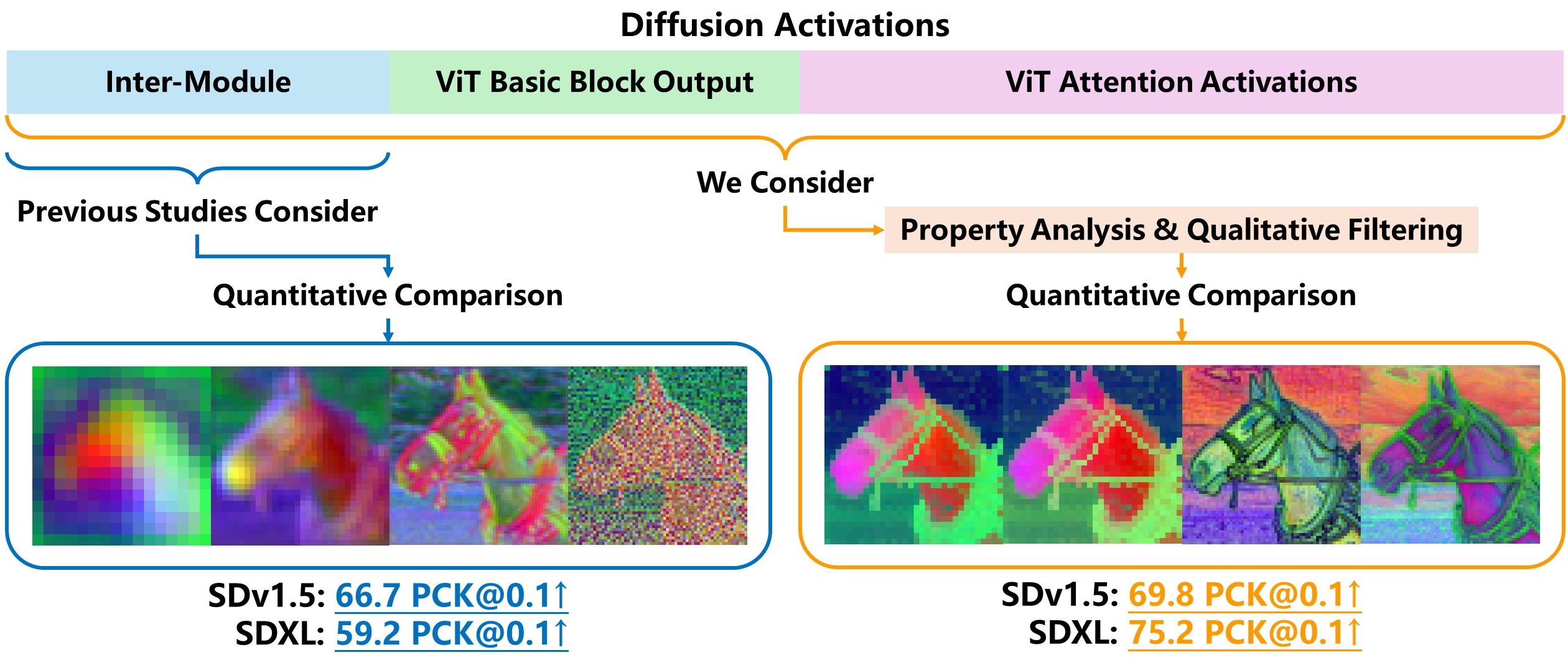
Figure 1: Prior arts only consider a small fraction of potential activations in diffusion models. As a result, more advanced diffusion architecture fails to achieve better performance (SDXL v.s. SDv1.5). In contrast, we consider a broader range of candidate activations. To facilitate the quantitative comparison, we first make a comprehensive and generalizable analysis to qualitatively filter out many candidates in advance. On top of this, our method achieves superior performance (75.2 PCK@0.1).

In this paper, we revisit the fundamental problem of feature selection, considering a more comprehensive candidate pool of activations. Due to its large volume, a full-scale quantitative comparison is no longer operational, urging us to modify the previous research methodology in [2]. As illustrated in Figure 1, instead of a direct quantitative comparison, we first explore the properties of diffusion U-Nets. These properties allow us to qualitatively and efficiently filter out many activations that are highly likely to be sub-optimal, shrinking the candidate pool for the quantitative comparison. More importantly, we find these properties are universal among diffusion models, making it possible to generalize our findings to more models beyond those covered in this paper.

Specifically, the properties we find, which are distinct to existing knowledge of model properties [1, 38], exactly correspond to three top-to-bottom levels of the diffusion U-Net: (i) Diffusion noises at the macro level: the diffusion process induces a new type of noise on both low- and high-frequency signals. (ii) In-resolution granularity changes at the in-resolution level: the changes in information granularity are not only across but also within resolutions. (iii) Locality without positional embeddings at the sub-module level: the embedded ViTs in diffusion U-Nets present a new type of local information different from that induced by the conventional positional embeddings [44]. Based on these insights, we develop effective feature selection solutions for several popular diffusion models. Finally, the experiments on three discriminative tasks, including semantic correspondence, semantic segmentation, and label-scarce segmentation, validate the superiority of our solutions over the SOTA methods.

In summary, the contributions of this work are three-fold:

• Revisit of a fundamental problem: To the best of our knowledge, we are the first to point out that the fundamental issue of feature selection remains unresolved in the realm of diffusion feature.

• Generic insights: The properties we find are universal among different diffusion U-Nets, which can provide valuable insights for future work.

• Extensive validation: Extensive experiments on three discriminative tasks validate the effectiveness of the feature selection solutions induced by our insights.

2 Related Work

Diffusion models for discrimination. We discuss three mainstream ways to use diffusion models for discrimination. (i) Diffusion classifier [26, 7] utilizes Bayes’ theorem to transform a pre-trained diffusion model into an image classifier. This method enjoys a theoretical guarantee and does not need additional training. However, it is limited to image-level tasks. (ii) The second way is to model discriminative tasks as image-to-image generation tasks with diffusion models [22, 23]. This method is suitable for various dense vision tasks but requires heavy training. (iii) Diffusion feature [2, 58, 56, 41, 29], the focus of this paper, follows the traditional practice of feature extraction to pursue the balance between wider applicability and less training. This makes it adaptable for different tasks and alleviates the training needs for the diffusion model. Only small downstream models may require training.

The diffusion feature approach has seen various improvements. Some techniques toggle the input settings of diffusion models, such as seeking better timesteps [60, 29]. The others add trainable parameters outside the diffusion model to refine the outputs or provide an efficient fine-tuning alternative [58, 27, 46]. Additionally, some studies explore completely training-free methods that utilize spatial attention information [51, 43], and some attempts focus on text-free diffusion models [32, 33].

Despite the progress, previous methods only consider activations between neighboring modules, leaving many potential candidates unevaluated. Our work shows that such an overlook can hinder model performance. By introducing a more comprehensive feature selection solution, our method could generically enhance both existing and future diffusion feature approaches.

Analysis on model properties. The inner properties of neural networks have consistently received much attention [5, 34]. For transformers, Geva et al. [15] show that the feed-forward layers act as key-value memories and are interpretable for humans. Amir et al. [1] extend this insight to vision transformers and put it into practical applications such as image classification, while Vilas et, al. [45] try to make more detailed interpretation of ViT activations.

The methodology of these studies provides valuable guidance for our research. However, since diffusion models are trained for generation, our study relies more on qualitative analysis and feature visualization compared to previous work.

3 Preliminaries: Architecture of Diffusion U-Nets

Diffusion models typically involve a forward pass and a reverse pass [21]. During the forward pass, noise is gradually added to a clean image $\boldsymbol{x}_{0}\in\mathbb{R}^{3\times w\times h}$ until the image resembles Gaussian noise, where $w$ and $h$ denote the width and height, respectively. This process can be denoted by $\boldsymbol{x}_{t}\sim q(\boldsymbol{x}_{t}|\boldsymbol{x}_{0})$, where $q$ represents the noise posterior and $t$ is the timestep. In the reverse pass, an end-to-end neural network $\epsilon_{\theta}$, as parameterized by $\theta$, learns to predict the noises and thus reconstruct the image. One such denoising step can be denoted as $\epsilon=\epsilon_{\theta}(\boldsymbol{x}_{t},t,\boldsymbol{c})$, where $\epsilon$ is the predicted noise, and $\boldsymbol{c}$ is the condition that describes the expected image content. Although there are alternative formulations for diffusion models [39, 28, 40], they all rely on this neural network backbone $\epsilon_{\theta}$. This study focuses on this backbone, typically implemented as U-Net [38], rather than other components of diffusion models. Next, we will detail the architecture of the diffusion U-Net and standardize the terminology referring to different parts of the model, as shown in Figure 2.

We start with an overview. Following the initial U-Net design [38], the U-Net has three main stages: down-stage, mid-stage, and up-stage. The down-stage reduces the resolution of activations, while the up-stage increases it. Both stages contain multiple resolutions, in each of which the activations share the same resolution. Furthermore, each resolution includes several modules, including ResModule (convolutional ResNet [20] structures), ViT Module [12], and Downsampler/Upsampler (simple convolutional layers). Previous diffusion feature approaches only consider activations between these adjacent modules, i.e., inter-module activations.

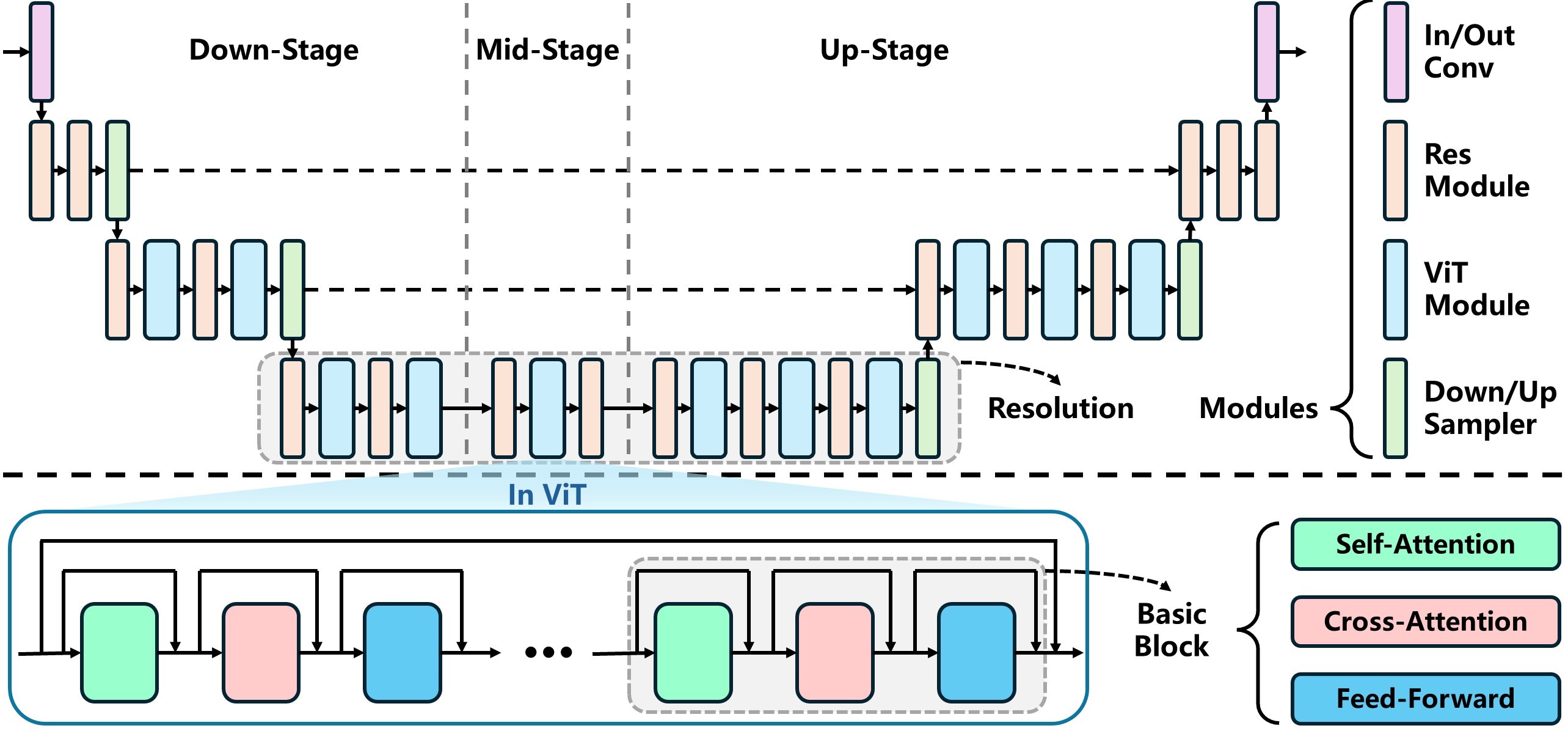
Figure 2: U-Net architecture (upper) and the ViT module (lower), taking SDXL as an example.

We next dive into the details below the module level. Among these modules, ResModule and ViTs adopt residual connection [20], where an increment activation is added element-wise to the residual activation to refine it. Specifically, ResModule uses simple convolutional layers to produce increments, whereas ViTs use complex attention mechanisms, which will be further explained next. Typically, ViT operates as a standalone model followed by a decoder that produces the output predictions for visual tasks [12, 25, 9, 18]. However, in the diffusion U-Net, multiple ViTs are embedded into the network, and their outputs serve as increment activations.

Furthermore, each ViT module consists of several stacked basic blocks. A basic block typically has a self-attention layer to perform attention on the image itself and a feed-forward layer, essentially a two-layer MLP [15]. Modern diffusion U-Net introduces an additional cross-attention layer between the two layers, enabling the fusion of the image and additional textual prompts. Besides, each layer includes a residual connection, meaning that the increment activation added to the outer residual is also the internal residual.

In a nutshell, the architecture described above provides abundant activations that can serve as dense features. Given the massive activations, it is no longer operational to perform a full-scale quantitative comparison. Hence, we next make a comprehensive analysis of model properties to better understand these activations, which can help the qualitative filtering.

4 Distinct Properties of Diffusion U-Nets

The diffusion U-Net has many interesting properties, but now we only focus on those distinct from the knowledge of traditional U-Net [38] or ViTs [44]. As shown in Figure 3, this section highlights three noticeable properties, each of which corresponds to a different level of the diffusion U-Net architecture described in Section 3. Notably, these properties can be universally observed in different samples and diffusion models, though all visualization in the main content is conducted on the same image and SDXL model for consistency. Additional visualization is provided in Appendix A. Besides, the omitted properties are available in Appendix E.

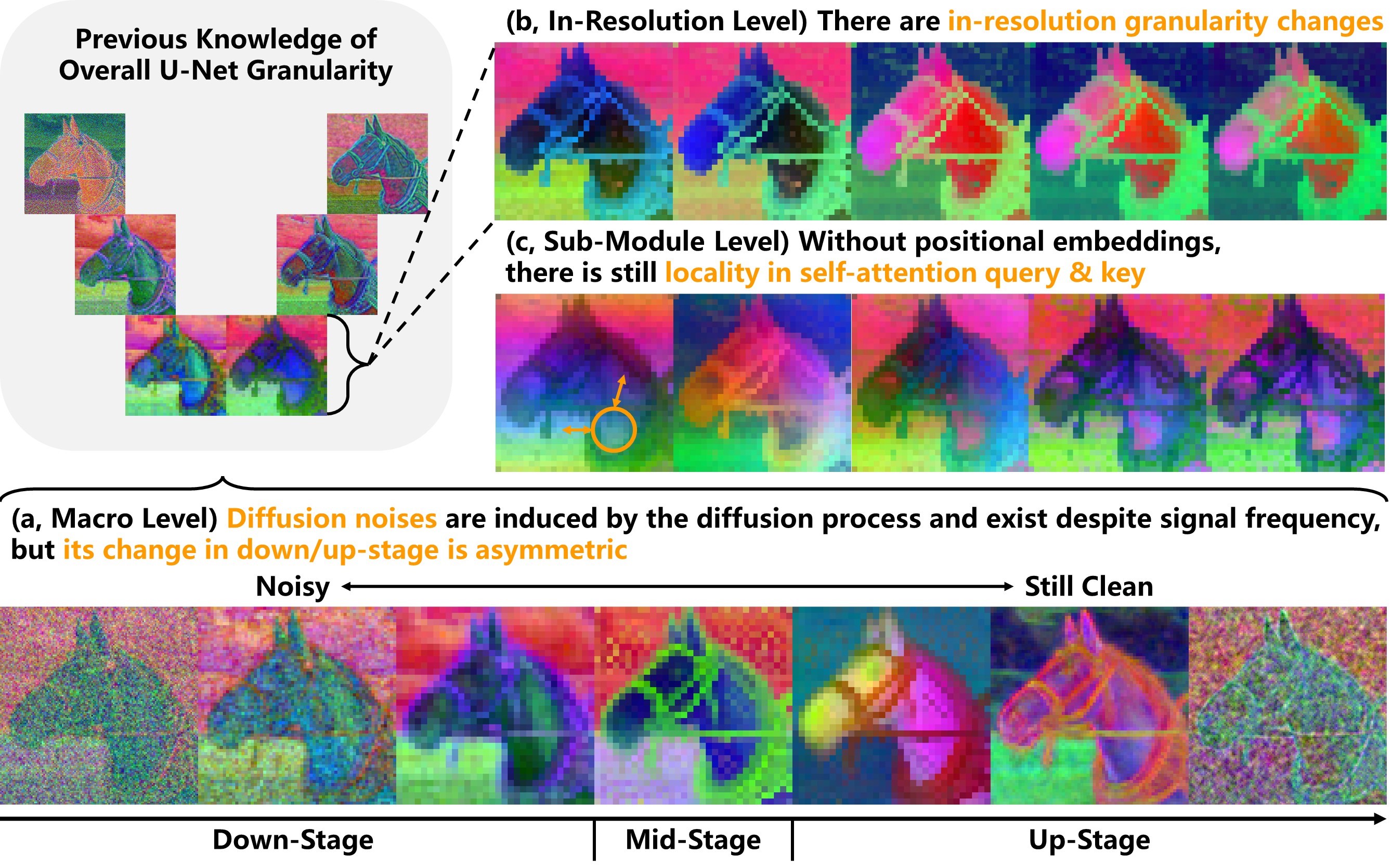
Figure 3: We highlight three properties of diffusion U-Nets that are distinct from existing knowledge about other models: (a) Asymmetric diffusion noises. (b) In-resolution granularity changes. (c) Locality without positional embeddings: pixels within the orange circle resemble nearby background pixels more than distant pixels on the horse’s neck that are semantically closer.

4.1 Asymmetric Diffusion Noises

The first property is at the macro level and closely related to the overall diffusion process. It is common that high-frequency signals are typically noisy [5, 34]. This phenomenon can also be observed in diffusion U-Nets, especially within the increment activations of residual connection. However, this does not mean that low-frequency signal activations in diffusion U-Nets are free from noises. As shown in Figure 3(a), the diffusion process introduces a new type of noise that also impacts low-frequency signals. This is not surprising since the diffusion process requires the backbone to process noisy inputs and predict noises as outputs. As a result, activations near the inputs or outputs, regardless of their frequency, also suffer from such noises. Considering the special cause, we name such noises diffusion noises.

How does the influence of diffusion noises spread across diffusion U-Nets? As shown in Figure 3(a), diffusion noises exist throughout the entire down-stage, with a decreasing magnitude. Remarkably, during the early half of the up-stage, activations are rather clean, with no perceivable diffusion noises. Only in the later half do diffusion noises start to resurface. The existence of this asymmetric behavior can also be indirectly supported by the ablation curves in many fellow studies such as [2, 32, 33]. Furthermore, as shown in Appendix A, such an asymmetric pattern is consistent across activations in different diffusion models.

Similar to common high-frequency noises, diffusion noises can degenerate feature quality. Hence, this property can serve as a criterion for identifying and filtering out sub-optimal activations, which we will delve into in Section 5.

4.2 In-Resolution Granularity Changes

The second property is at the in-resolution level and closely related to recent advances in diffusion architectures. Specifically, the design of U-Net follows the idea of resolution hierarchy [38]. Consequently, the overall architecture displays a fine-coarse-fine granularity trend, looking like the alphabet “U”. Traditional U-Nets implement this architecture with a relatively large number of resolutions, while each resolution is typically small, equipped with two or three simple convolutional layers. Hence, the understanding of traditional U-Net focuses on the granularity changes across resolutions, implicitly assuming that the change within a single resolution is negligible.

However, diffusion U-Nets become much “fatter”. In other words, modern diffusion U-Nets typically have much fewer resolutions, but each resolution is significantly enlarged. For example, SDv1.5 only has four resolutions [37], and SDXL further decreases this number to three [36], as shown in Figure 2. Meanwhile, each resolution can produce much more activations, primarily thanks to the embedded ViT modules. This architectural evolution makes the granularity change within a single resolution more significant, as depicted in Figure 3(b).

Different granularity carries varied information and quality, resulting in different discriminative performance on downstream tasks [2, 29]. Hence, this discovery of in-resolution granularity changes highlights the necessity to evaluate more activations, especially those within the embedded ViTs, as they are of different granularity.

4.3 Locality without Positional Embeddings

For the third distinct property, we delve into the sub-module level, i.e., the blocks in embedded ViT modules. Positional embeddings, which are widely used in language transformers [44] and ViTs [12], aim to provide spatial information for each input token. Consequently, the activations of traditional ViTs display strong positional information, where the latent pixel resembles nearby pixels more than those that are semantically similar but far away [1]. This phenomenon is significant for the layers close to the inputs. When the layer goes deeper, the tokens are refined with semantic information, making the activations display less positional information. However, only in the last few layers, such positional information becomes negligible.

In contrast, ViT modules in diffusion U-Nets do not use positional embeddings [37, 36], perhaps because the other U-Net components have provided sufficient spatial cues. This change results in distinct properties of the activations. On one hand, positional information is negligible for most activations despite how near they are to the inputs. For example, even in the first basic block, cross-attention query activations contain no perceivable positional information. On the other hand, the queries and keys of self-attention still display non-negligible positional information, marked with orange circles in Figure 3(c). Specifically, the latent pixel on the horse’s neck is a light blue color, similar to the pixels to its left that actually represent the background. In contrast, the pixels above the circle are in purple color, though they also represent the horse’s neck. Such comparison shows that a latent pixel is more similar to other pixels that are spatially near it than those semantically closer to it.

We name this phenomenon locality since it has a different mechanism from that induced by positional embeddings. As pointed out in [12], self-attention allows ViT to integrate global and local information even in the shallow layers, and the attention scope enlarges w.r.t. layer depth. Even without positional embeddings, self-attention activations are generally consistent with this insight, leading to the existence of locality. Nevertheless, the magnitude has indeed greatly reduced, compared to the visualization of conventional ViT activations in  [1]. As shown in Figure 3(c), in shallow activations, locality exists but is inherently weaker, as much semantic information is still reserved. In addition, locality quickly diminishes as the layer goes deeper.

Since positional information can degrade the quality of activations [1], its absence has the potential to enhance the activations in ViT modules. Moreover, locality can play a special role in activation filtering, as presented in Section 5.

4.4 Universality of Three Properties

Although the visualization in Figure 3 is conducted only on SDXL, the scope of these properties is not limited to the specific architecture. Further supporting evidence is available in Appendix A.

1. Diffusion noises directly arise from the diffusion process. Hence, it is promising to extend this property to other diffusion backbones.

2. In-resolution granularity changes come from the “fatness” of U-Nets, making it potentially applicable to more traditional U-Nets.

3. Locality originates from the self-attention mechanism in ViT architectures, so it is broadly applicable to standalone or embedded ViTs where positional embeddings are absent.

5 Enhanced Feature Selection from Diffusion U-Nets

So far, we have had a more comprehensive understating of the properties of diffusion U-Nets. All these properties, especially in-resolution granularity changes, encourage us to reconsider the feature selection solution, with a special emphasis on the activations in ViT modules. With these properties, we are also able to filter out many low-quality activations qualitatively, followed by a thus simplified quantitative comparison.

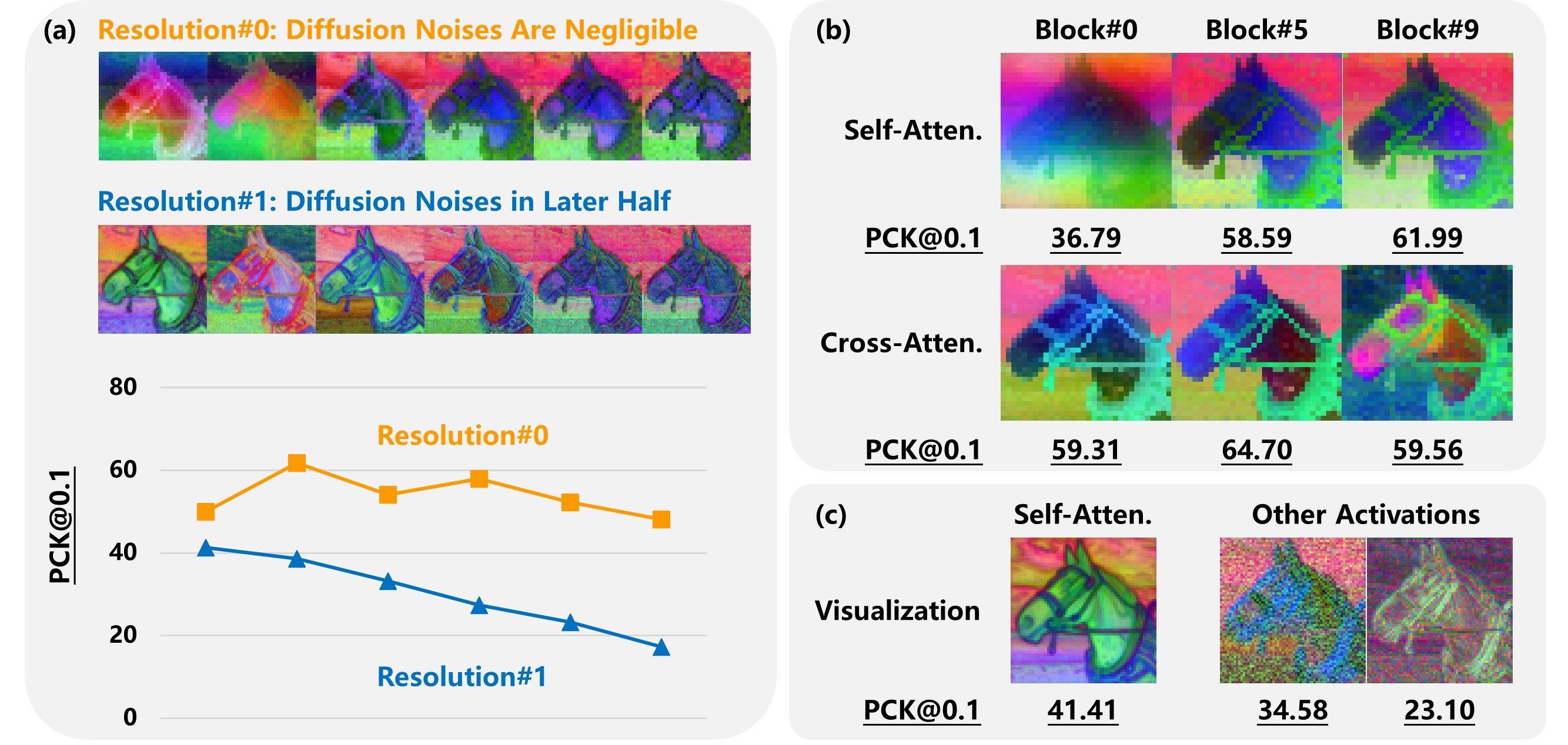
Figure 4: (a) Diffusion noises result in a significant performance degeneration ( Resolution#1). (b) Locality degrades the quality of self-attention activations (Block#0 and Block#5). (c) Locality in self-attention activations can suppress diffusion noises, leading to better quality than noisy activations (41.41 v.s. 34.58). All $\text{PCK@0.1}_{\text{img}}(\uparrow)$ results are evaluated on the semantic correspondence task.

5.1 Qualitative Filtering

Avoiding Diffusion Noises. As shown in Figure 4(a), diffusion noises tend to degrade the quality of activations. Hence, it is natural to filter out the activations severely affected by diffusion noises from the candidate pool. Specifically, according to the asymmetric trend of diffusion noises, we only consider activations in the early half of the up-stage, which are rather clean. This approach will significantly reduce the number of candidate activations and simplify the quantitative comparison.

Avoiding Self-Attention Locality. The locality in self-attention modules is another important factor that can degrade the activations. The empirical evidence in Figure 4(b) demonstrates that these activations are generally inferior to the others, such as those from cross-attention layers or the outputs of ViT basic blocks. Consequently, it is rather safe to filter out most activations in self-attention modules from our candidate pool.

Using Locality to Suppress Diffusion Noises. So far, the activations in the candidate pool are clean and free from locality. However, all these activations are low-resolution ones since high-resolution activations are generally noisy and thus filtered out. This is unfavorable since some detailed information might only exist in high-resolution activations. To address this issue, we exploit a side effect of self-attention locality. Specifically, as indicated in Figure 4(c), locality can help suppress diffusion noises via its focus on spatial structures. Although locality is sub-optimal, it is still superior to severe diffusion noises. In view of this, the candidate pool reserves self-attention activations extracted from the later half of the up-stage.

We have filtered out many candidate activations based on the distinct properties of diffusion U-Nets. Additionally, all increment activations in residual connection can be further filtered out since they introduce high-frequency noises [5, 34]. After such qualitative filtering, a small but high-quality candidate pool is available. Taking SDXL as an example, the number of candidates decreases from 279 to 63, i.e., a 78% reduction. Next, we explain how to conduct this quantitative comparison briefly.

5.2 Quantitative Comparison

The quantitative comparison follows the protocol of [2]. Specifically, given an input image $\boldsymbol{x}_{0}$, we first perform the forward pass with a pre-defined timestep $t$ to generate the noisy image $\boldsymbol{x}_{t}$. Then, the U-Net backbone conducts one denoising step. Instead of collecting the model output $\epsilon$, we gather U-Net activations and consolidate them to the candidate pool, as described in Section 5.1. Afterward, each activation is individually fed to a downstream model to evaluate its discriminative potential, with the details of the model described in Appendix C. Such comparison is made fair by using the same dataset for all activations. Finally, we can obtain the capability ranking of activations from each resolution, according to which features can be selected wisely. Notably, we conduct such comparisons on multiple datasets to guarantee generalizability, since the best activations may differ among different scenes [2]. Thanks to qualitative filtering, the time cost for each (model, dataset) pair has been reduced by more than one week, equipped with Nvidia(R) RTX 3090 GPUs.

Given the capability ranking, feature selection is in fact flexible, as it is possible to combine multiple activations and specifically tune the choice for a task. For practicality, we provide off-the-shelf feature combinations for SDv1.5 and SDXL that are likely to generically perform well in Appendix B, according to the results detailed in Appendix D. Each of them consists of four activations mainly from ViT modules rather than inter-module positions. Taking SDv1.5 as an example, one of the four selected features is from one self-attention layer in the highest resolution, which utilizes our observation in Section 4.

6 Experimental Validation on Multiple Discriminative Tasks

Table 1: Experimental results on the semantic correspondence task. The best results are in bold font and the runner-up is underlined.

Category	Method	$\text{PCK@0.1}_{\text{img}}\uparrow$	$\text{PCK@0.1}_{\text{bbox}}\uparrow$
SOTA	DINO	51.68	41.04
	DHPF	55.28	42.63
	DIFT	-	52.90
	DHF	72.56	64.61
Baseline	Legacy-v1.5	75.14	66.73
	Legacy-XL	66.00	59.16
Ours	Ours-v1.5	77.78	69.83
	Ours-XL	81.72	75.18
	Ours-XL-t	83.90	76.86

To validate the effectiveness of our feature selection solution, the experiments are conducted on three popular discriminative tasks: semantic correspondence, semantic segmentation, and label-scarce segmentation. The SOTA methods for each task are selected as competitors. Besides, we also compare with two baselines that select the conventional inter-module activations as features [2], named Legacy-v1.5 and Legacy-XL. For our method, we provide the following implementations:

• Ours-v1.5 & Ours-XL: Features extracted from SDv1.5 and SDXL, respectively.

• Ours-XL-t: For fairness, we further enhance SDXL features with some additional techniques that are also adopted by SOTAs. The techniques we select, i.e., attention maps [58] and feature amalgamation [2, 29, 60], are relatively simple and lightweight.

More experimental details are in Appendix C, such as task information, evaluation metrics, and implementation details. Besides, Appendix D presents additional results not covered here.

6.1 Empirical Results on Semantic Correspondence

We present the experimental results for semantic correspondence in Table 1. From the results, we have the following observations:

1. Ours-v1.5 outperforms Legacy-v1.5 (77.78 v.s. 75.14 on $\text{PCK@0.1}_{\text{img}}$). The main reason is that Legacy-v1.5 fails to effectively handle the diffusion noises in high-resolution activations. Previous approaches either reserve the noisy activations and thus suffer from performance degradation [2, 52], or simply discard high-resolution activations and thus suffer from information loss [58, 46]. In contrast, our approach uses self-attention locality to suppress diffusion noises and harvest better high-resolution activations.

2. Legacy-XL is inferior to Legacy-v1.5 (66.00 v.s. 75.14 on $\text{PCK@0.1}_{\text{img}}$). At first glance, this result is counter-intuitive since SDXL is more advanced than SDv1.5. However, the analysis in Section 4 can unravel the mystery. Specifically, since SDXL has more ViT modules, the more valuable activations shift from inter-module positions to these embedded ViTs. Since the baseline does not consider ViT modules, Legacy-XL fails to achieve better performance. In contrast, Ours-XL shows improvement over Ours-v1.5 (81.72 v.s. 77.78 on $\text{PCK@0.1}_{\text{img}}$). This is consistent with the advance in model architecture and again validates our analysis.

3. Ours-XL-t significantly outperforms the SOTA method with a similar amalgamation technique, i.e., DHF [29] (83.90 v.s. 72.56 on $\text{PCK@0.1}_{\text{img}}$). This performance gain again validates the effectiveness of our method.

Table 2: Experimental results on semantic segmentation and its altered version with scarce labeled data, evaluated using mIoU$\uparrow$ metric. The best results are in bold font and the runner-up is underlined.

Category	Method	Standard Setting		Method	Label-Scarce Setting
		ADE20K	CityScapes		Horse-21
SOTA	MaskCLIP	23.70	-	SwAVw2	54.0 ± 0.9
	ODISE	29.90	-	MAE	63.4 ± 1.4
	VPD	37.63	55.06	DatasetDDPM	60.8 ± 1.0
	Meta Prompts	40.89	71.94	DDPM	65.0 ± 0.8
Baseline	Legacy-v1.5	40.26	64.01	Legacy-v1.5	59.4 ± 1.3
	Legacy-XL	27.78	71.67	Legacy-XL	53.0 ± 0.9
Ours	Ours-v1.5	41.07	64.10	Ours-v1.5	60.2 ± 0.9
	Ours-XL	43.45	74.47	Ours-XL	62.7 ± 0.7
	Ours-XL-t	45.71	75.89	Ours-XL-t	66.3 ± 0.9

6.2 Empirical Results on Semantic Segmentation

As shown in the left part of Table 2, Ours-XL-t and Ours-XL achieve state-of-the-art performance on the semantic segmentation task (45.71 and 43.45 v.s. 40.89 on ADE20K), demonstrating its effectiveness and generalizability. Furthermore, the most competitive SOTA, Meta Prompts [46], introduces a large number of trainable parameters and uses the diffusion U-Net recurrently, which is rather time-consuming. In contrast, our method delivers superior results with efficiency maintained.

Unlike the results in semantic correspondence, Legacy-XL outperforms Legacy-v1.5 on CityScapes (71.67 v.s. 64.01), and the performance gap between Legacy-v1.5 and Ours-v1.5 is narrow (64.01 v.s. 64.10). This is because this task utilizes a relatively large-scale downstream model, which can significantly refine the input features and thus reduce the gap in feature quality. Nevertheless, Ours-XL still achieves a significant improvement over Legacy-XL (74.47 v.s. 71.67).

6.3 Empirical Results on Label-Scarce Segmentation

One advantage of diffusion features is the applicability to label-scarce scenarios [2]. For validation under such conditions, we experiment on the label-scarce segmentation task, with results presented in the right part of Table 2. The observations are generally similar to those on the semantic correspondence task. For example, Ours-v1.5 outperforms Legacy-v1.5 (60.2 v.s. 59.4), Legacy-XL is inferior to Legacy-v1.5 (53.0 v.s. 59.4), and Ours-XL is better than Ours-v1.5 (62.7 v.s. 60.2).

Next, we focus on the comparison with the SOTA method, DDPM [2]. Although DDPM is a relatively early study, it outperforms the other competitors and our most implementations. This result has two reasons. On one hand, DDPM performs the diffusion process directly in the image space rather than the currently common practice of compressed latent space. Although inefficient, such an implementation yields better discriminative features. On the other hand, DDPM utilizes diffusion models specifically trained on each dataset. In comparison, we use pre-trained general-purposed SDv1.5 or SDXL to be more efficient and thus consistent with the motivation of diffusion feature. Hence, it is rather challenging to surpass this SOTA method. Fortunately, our best implementation, Ours-XL-t, achieves this goal with the help of additional lightweight techniques (66.3 v.s. 65.0).

7 Conclusion and Future Work

In this study, we revisit the fundamental problem of feature selection from diffusion U-Nets. We point out that prior arts only consider a limited range of potential activations. In contrast, we consider a much wider range of activations as candidates, especially those extracted from the embedded ViT modules. Given the large volume of the candidate pool, we first analyze the properties of diffusion U-Nets. The properties we find are universal such that our observations are not limited to the specific diffusion architecture. Based on these properties, we qualitatively filter out many activations with low quality, facilitating the following quantitative comparison. On top of this, concrete feature selection solutions are proposed for two popular diffusion models, i.e., SDv1.5 and SDXL. Finally, extensive experiments on three discriminative tasks validate the effectiveness of our method.

However, we are not sure whether our observations can generalize well to recently-developed DiT models [35] since they have a markedly different architecture from U-Net-based diffusion models. Thus, analyzing DiT models is a promising topic for future research.

Contents

[appendices] [appendices]l1

Appendix A Additional Visualization for Distinct Properties of Diffusion U-Nets

A.1 Visualization of Other Sample Images

We have provided activation visualization from SDXL in a simple outdoor scene presenting a horse in the wild. Next, we will show visualization from the same model in different scenes to demonstrate the universality of the observed properties. Another simple outdoor scene presenting a cat is in Figure 5. Two simple indoor scenes are visualized in Figure 6 and Figure 7. Two complex outdoor scenes of urban streets are visualized in Figure 8 and Figure 9. Two complex indoor scenes are shown in Figure 10 and Figure 11.

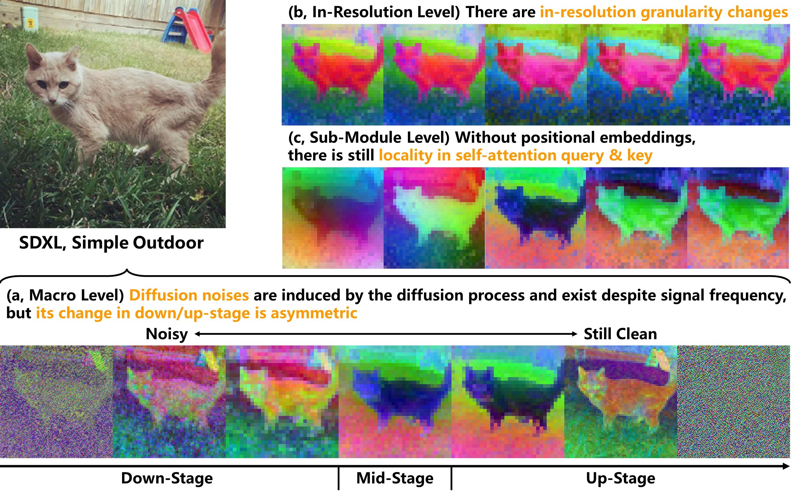
Figure 5: Visualization of SDXL activations on a simple outdoor scene.

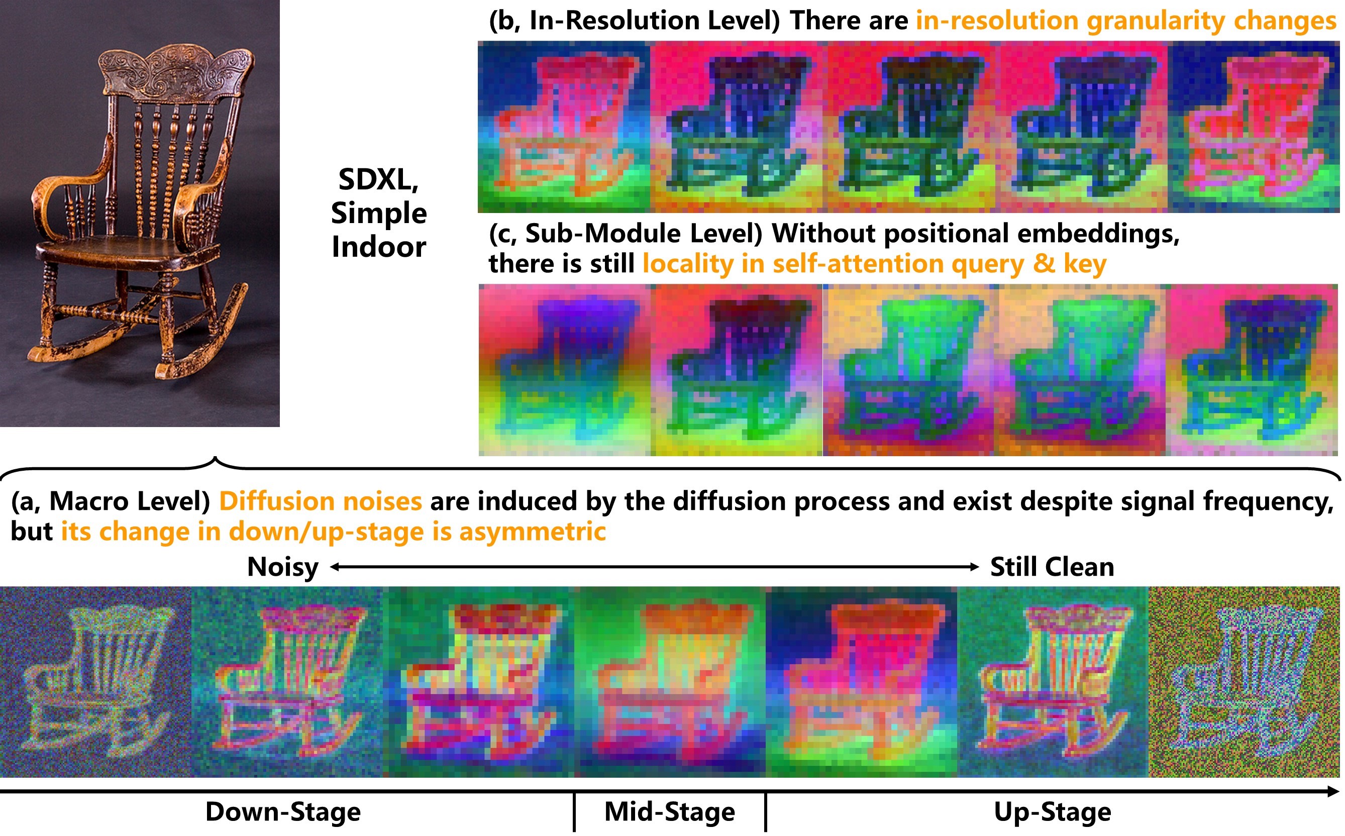
Figure 6: Visualization of SDXL activations on a simple indoor scene.

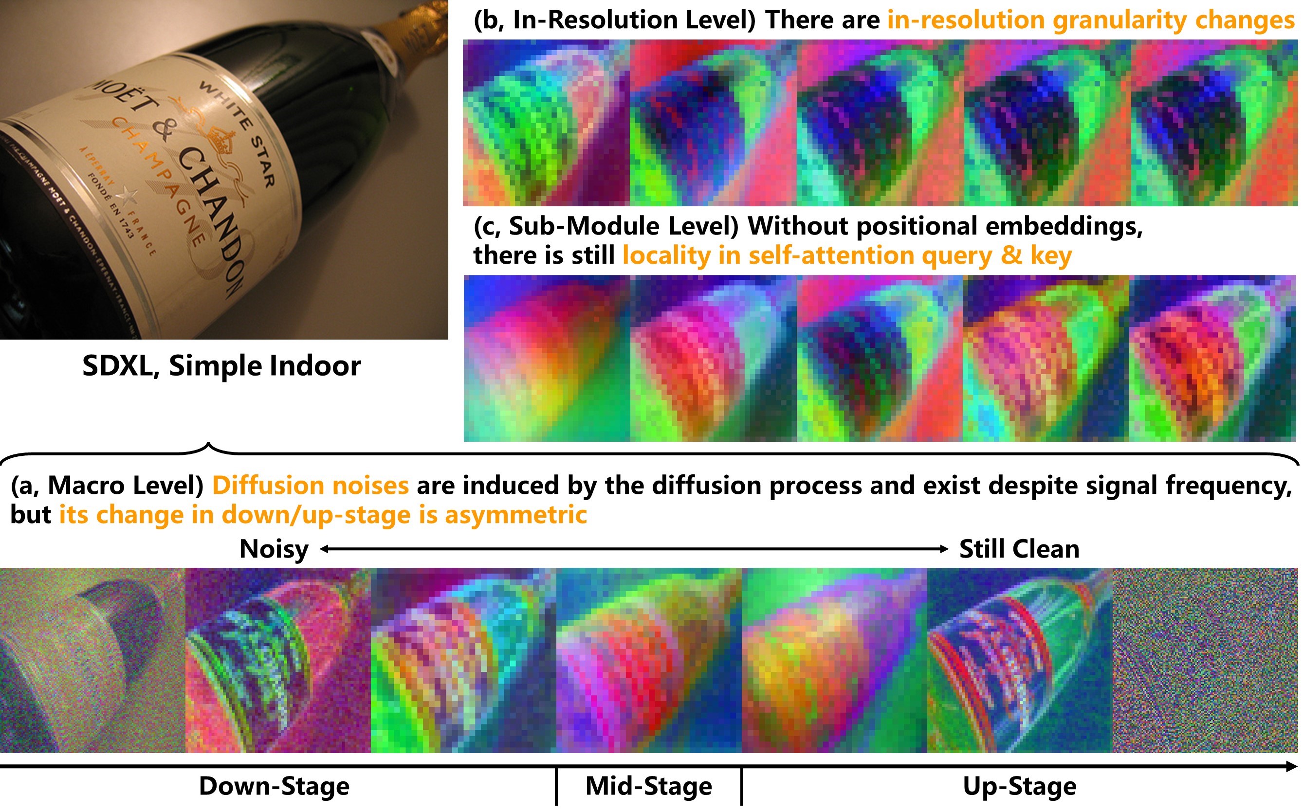
Figure 7: Visualization of SDXL activations on a simple indoor scene.

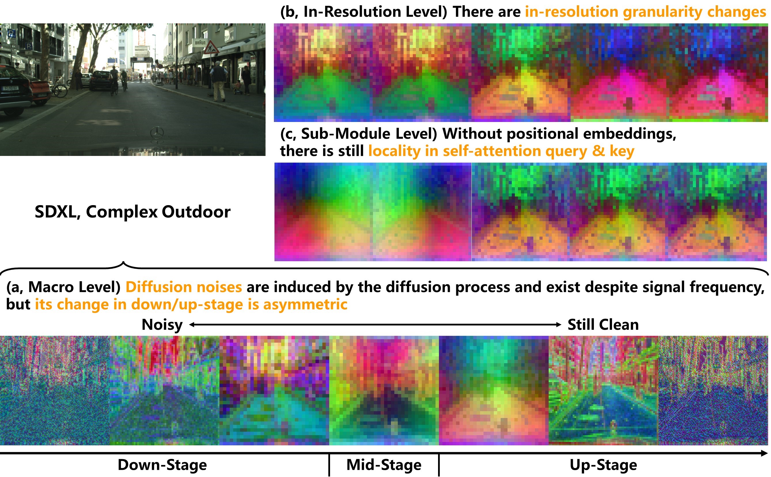
Figure 8: Visualization of SDXL activations on a complex outdoor scene.

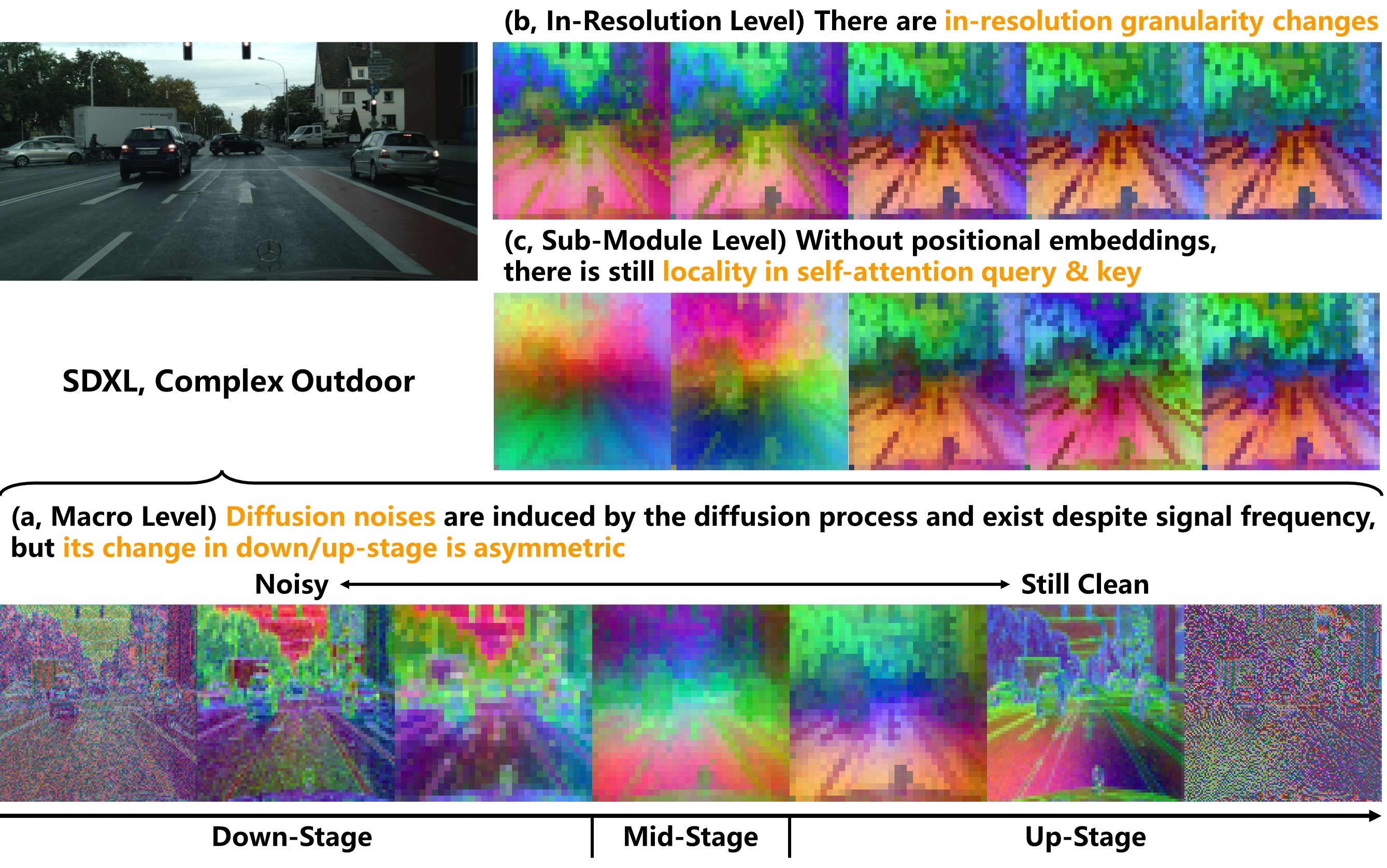
Figure 9: Visualization of SDXL activations on a complex outdoor scene.

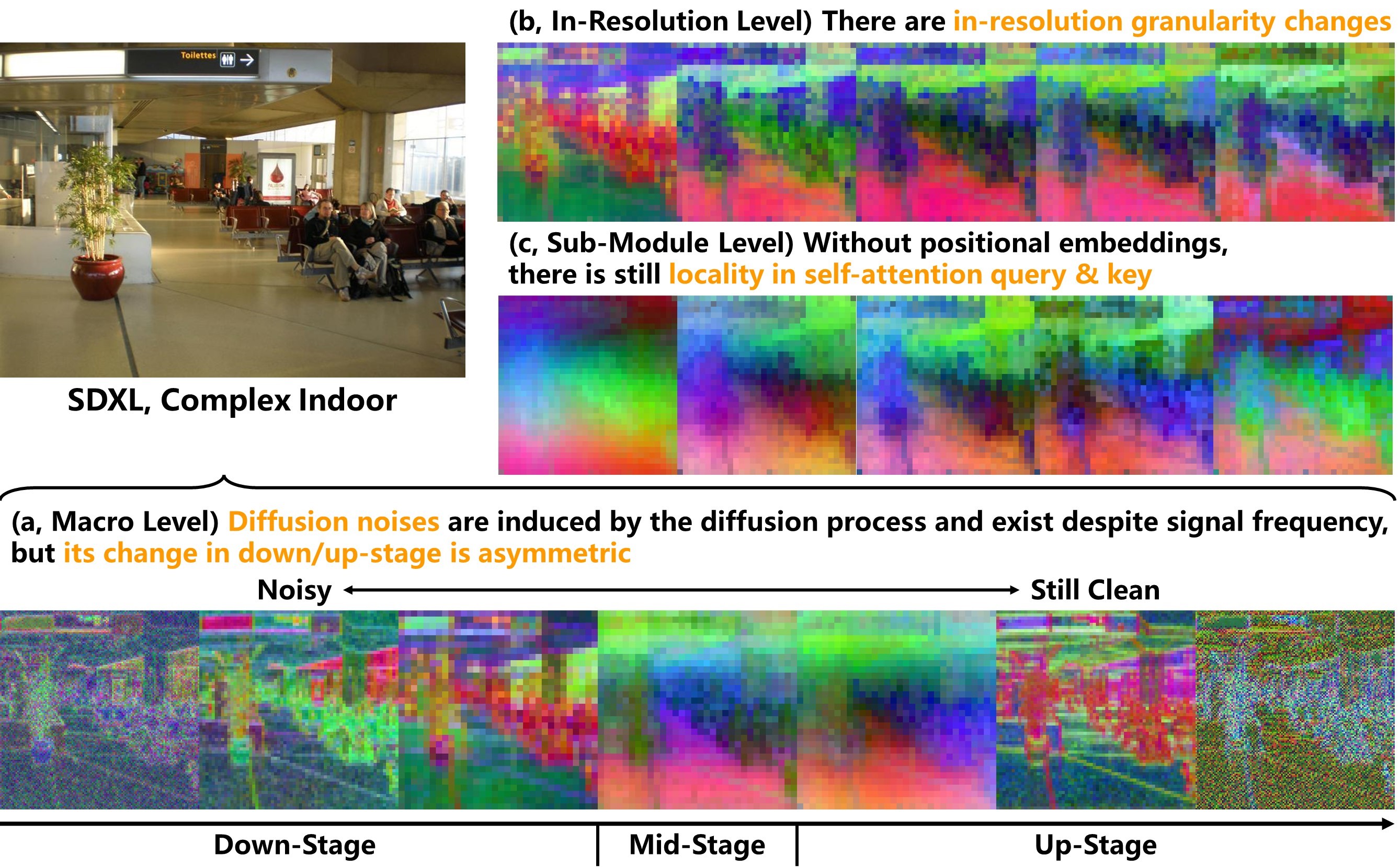
Figure 10: Visualization of SDXL activations on a complex indoor scene.

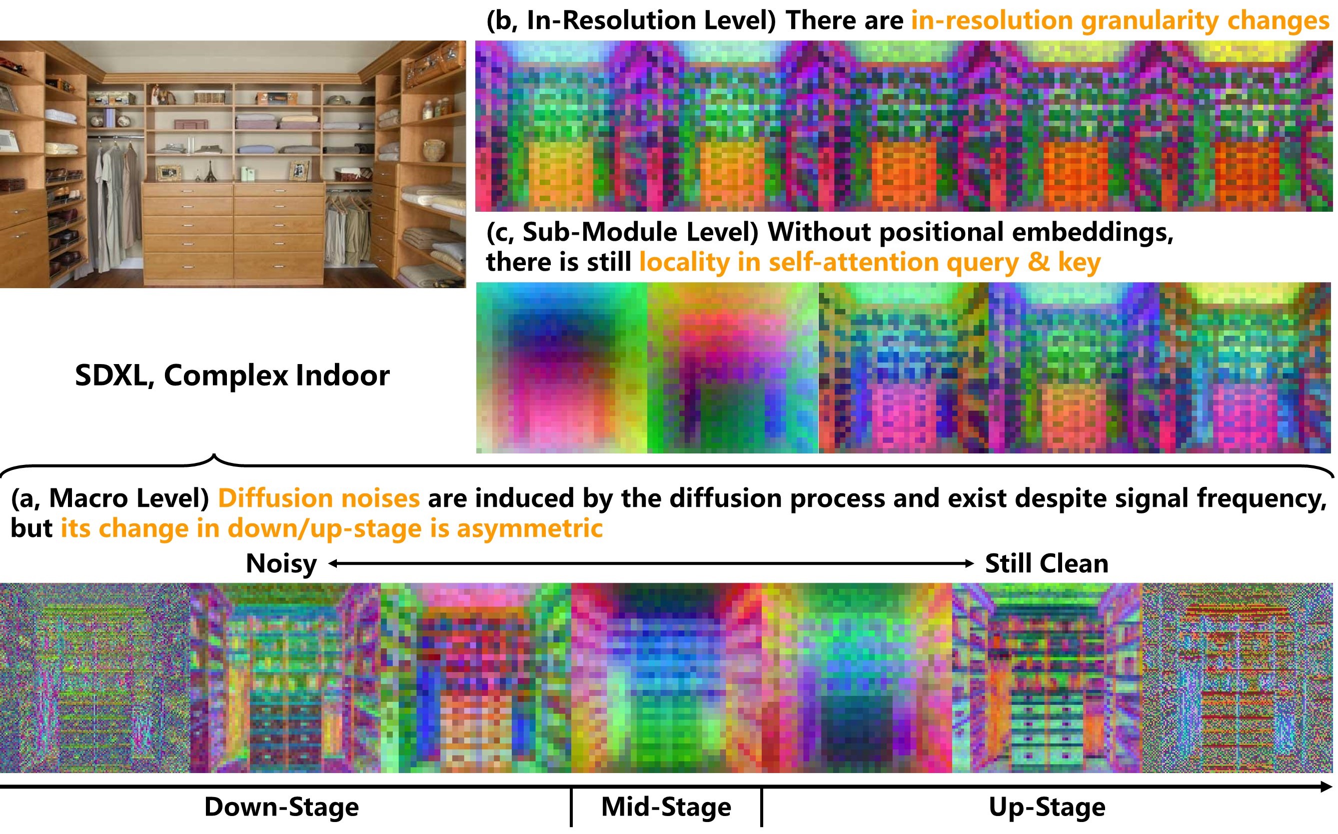
Figure 11: Visualization of SDXL activations on a complex indoor scene.

A.2 Visualization from Other Diffusion Models

Playground v2 Activations. Playground v2 shares the same architecture as SDXL but is trained independently, and it is claimed to be more powerful in generation. In Figure 12, we present its activation visualization using the same horse image as the primary SDXL visualization. Compared to SDXL, Playground v2 activations are less noisy, particularly in the down-stage. This supports the claim that Playground v2 is a stronger model.

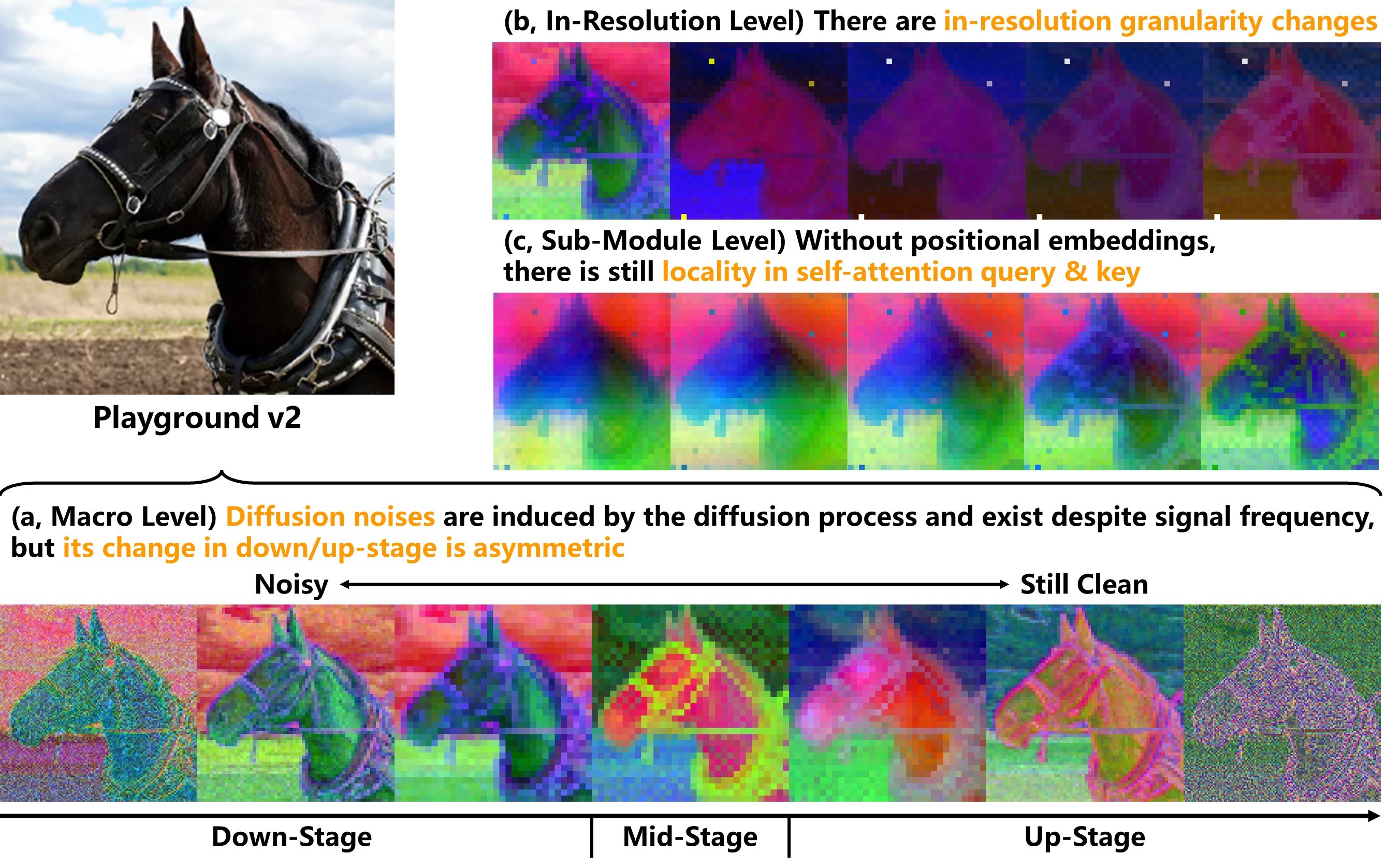
Figure 12: Visualization of Playground v2 activations on a simple outdoor scene.

SDv1.5 Activations. SDv1.5, as an older model, has a slightly different architecture from SDXL. Specifically, SDv1.5 has four resolutions instead of three, but its ViTs contain only one layer. Moreover, in SDXL, only the highest resolution lacks ViT due to efficiency concerns, while in SDv1.5, only the lowest resolution lacks ViT due to its low resolution. Despite the architectural changes, the three unique properties still apply to SDv1.5, as shown in Figure 13.

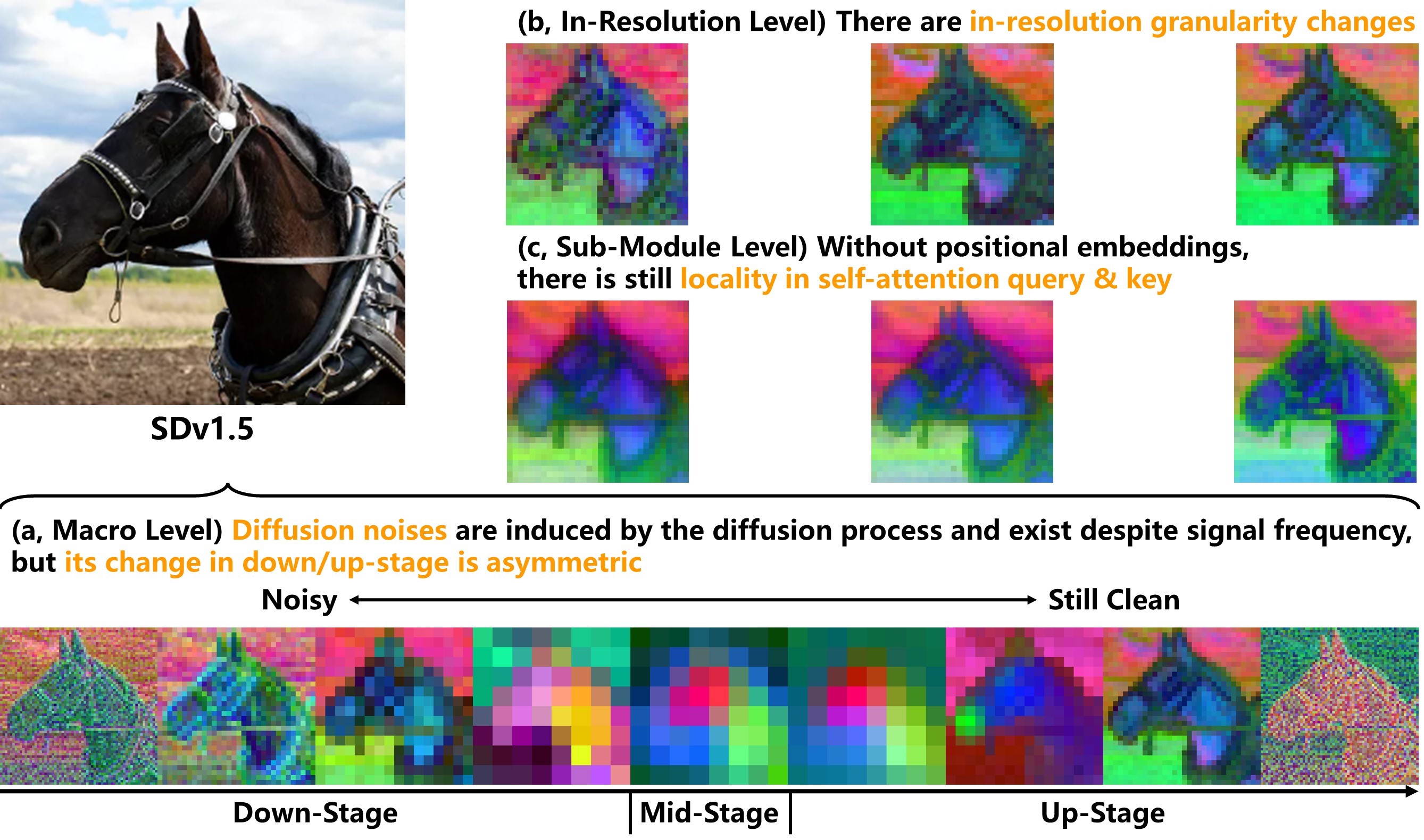
Figure 13: Visualization of SDv1.5 activations on a simple outdoor scene.

Video Diffusion Activations. To further demonstrate the universality, we even select a diffusion model for video generation [6] for visualization. This model is based on the SDv1.5 architecture, with an additional temporal attention layer inserted after cross-attention to enable sequential generation. Although this model is designed for a different task, we can still observe the three unique properties in Figure 14.

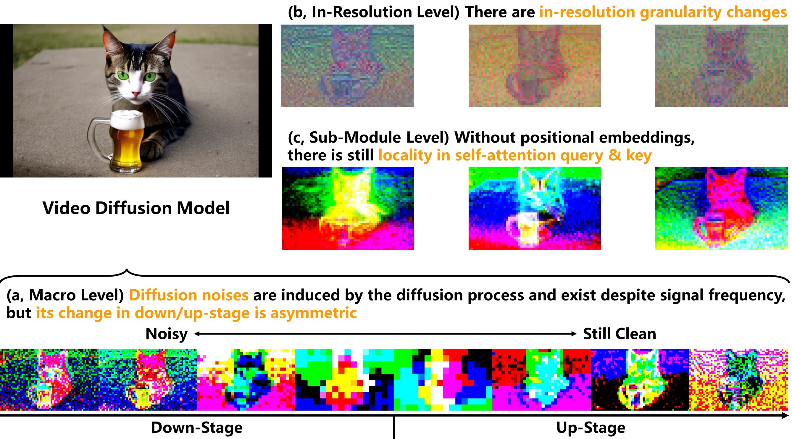
Figure 14: Visualization of the activations of a video diffusion model. The input is a short video, and we visualize one frame of it.

Conventional U-Net Activations. As comparison to diffusion U-Net, we also visualize some activations from a conventional U-Net in Figure 15, where the three properties of diffusion U-Net can hardly be observed.

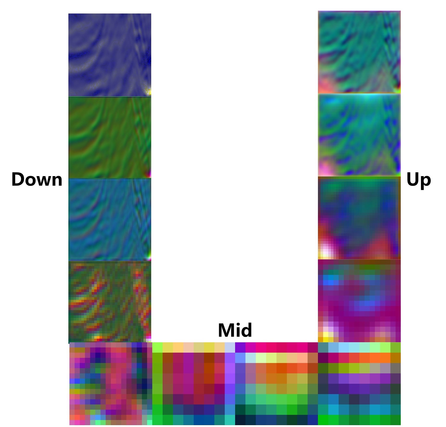
Figure 15: Activation visualization from a traditional U-Net for semantic segmentation [57].

Appendix B Details of Our Method

In this section, we index all diffusion U-Net components in the order in which they are activated during a network forward run. Besides descriptions in natural language, we also index the activations using the same notations as used in our code implementation. These notations denote stages using down/mid/up, resolutions as level, and module index as repeat. Index starts to count from 0 instead of 1, following the convention in coding.

B.1 Feature Selection Solution for SDv1.5

We select four activations from SDv1.5, maintaining the same total feature channels as the conventional way to extract all output activations from each resolution.

1. The cross-attention query activation from the 2nd ViT, the 2nd resolution. This provides coarse information for simple scenes (up-level1-repeat1-vit-block0-cross-q).

2. The inter-module activation after the 3rd ResModule, the 2nd resolution. This provides coarse information for complex scenes (up-level1-repeat2-res-out).

3. The cross-attention query activation from the 2nd ViT, the 3rd resolution. This provides finer information with a higher resolution (up-level2-repeat1-vit-block0-cross-q).

4. The self-attention key activation from the 1st ViT, the 4th resolution. This extracts features from the highest resolution, harnessing the noise suppression effect of self-attention locality (up-level3-repeat0-vit-block0-self-k).

We omit the index of basic blocks in ViTs, as SDv1.5 only contains one-layer ViTs. Additionally, we totally ignore the lowest resolution, as its activations have very low resolution ($8\times 8$ if the input image is $512\times 512$), suggesting inferiority, as supported by the quantitative comparison.

B.2 Feature Selection Solution for SDXL

Four activations are selected from SDXL, trying to get similar total feature channels to the SDv1.5 feature selection solution.

1. The output activation after the 8th basic block, the 1st ViT, the 1st resolution. This provides relatively coarse information for simple scenes (up-level0-repeat0-vit-block7-out).

2. The output activation after the 6th basic block, the 1st ViT, the 1st resolution. This provides relatively coarse information for complex scenes (up-level0-repeat0-vit-block5-out).

3. The cross-attention query activation from the 1st basic block, the 1st ViT, the 2nd resolution. This provides relatively fine information for simple scenes (up-level1-repeat0-vit-block0-cross-q).

4. The output activation after the 1st basic block, the 1st ViT, the 2nd resolution. This provides relatively fine information for complex scenes (up-level1-repeat0-vit-block0-out).

We ignore the highest resolution since it is affected by diffusion noises and lacks ViTs from which we can extract self-attention activations. However, if the downstream model is strong enough to learn to suppress noises, it may be possible to additionally extract inter-module activations from this resolution to harness more information.

B.3 Feature Selection Solution with Additional Techniques

For the setting Ours-XL-t, we mainly utilize two simple techniques that are also adopted in some SOTA methods: (i) We additionally extract attention maps, i.e., the similarity scores of cross-attention query and key, as dense features [58, 52]. Such attention maps are closely related to the semantics of prompts, thus providing important supplementary information. Despite its usefulness, this technique only adds a few additional channels to the features. (ii) We amalgamate features from different models [2, 29, 60] through simple concatenation. This technique is a common practice and can be seen as an extension of amalgamating different activations together as a whole feature. We next explain what activations are selected to implement the two techniquess.

We first extract features according to the feature selection solution for SDXL. Afterward, we extract additional features from SDv1.5:

1. The cross-attention query activation from the 2nd ViT, the 2nd resolution (up-level1-repeat1-vit-block0-cross-q).

2. The cross-attention query activation from the 2nd ViT, the 3rd resolution (up-level2-repeat1-vit-block0-cross-q).

3. The upsampler output activation from the 3rd resolution, to harness high-resolution information (up-level2-upsampler-out).

4. The self-attention key activation from the 1st ViT, the 4th resolution, to harness high-resolution information (up-level3-repeat0-vit-block0-self-k).

5. The attention maps averaged over all cross-attention layers in the up-stage.

We also extract one feature from Playground v2: the output activation after the 4th basic block, the 1st ViT, the 1st resolution (up-level0-repeat0-vit-block3-out).

B.4 Alternative Feature Selection Solution with Additional Techniques

Large-scale datasets for semantic segmentation mostly consist of images of complex scenes. In such cases, we find attention maps can be too noisy to be useful. Therefore, we discard the attention map technique and the entire SDv1.5 model, as it is weaker compared to the newer SDXL and Playground v2 models. To compensate for the loss of activations, we select additional activations from SDXL and Playground v2.

From SDXL, we select all the activations as described in the feature selection solution for SDXL and select one additional activation: the upsampler output activation from the 2nd resolution, to harness high-resolution information (up-level1-upsampler-out). From Playground v2, we select the following activations:

1. The output activation after the 6th basic block, the 1st ViT, the 1st resolution (up-level0-repeat0-vit-block5-out).

2. The cross-attention query activation from the 1st basic block, the 1st ViT, the 2nd resolution (up-level1-repeat0-vit-block0-cross-q).

3. The upsampler output activation from the 2nd resolution (up-level1-upsampler-out).

Appendix C Experimental Details

C.1 Semantic Correspondence

Task and Dataset. Semantic correspondence [18] involves finding a pixel in an image that semantically matches another keypoint pixel in a reference image, such as the hind legs of two different cats. We conduct experiments on the SPair-71k dataset [30].

Evaluation Metric. $\text{PCK@0.1}_{\text{img}}(\uparrow)$ and $\text{PCK@0.1}_{\text{bbox}}(\uparrow)$ are used, following the widely-adopted protocol reported in [30]. These two metrics mean the percentage of correctly predicted keypoints, where a predicted keypoint is considered to be correct if it lies within the neighborhood of the corresponding annotation with a radius of $0.1\times max(h,w)$. For $\text{PCK@0.1}_{\text{img}}$/$\text{PCK@0.1}_{\text{bbox}}$, $h,w$ denote the dimension of the entire image/object bounding box, respectively.

SOTA Competitors. We provide the results from four SOTA methods: DINO [4] and DHPF [31] as non-diffusion-feature methods, as well as DIFT [41] and DHF [29] as diffusion feature methods.

Implementation Details. The semantic correspondence task can be done via the nearest neighbor algorithm [42], which is unsupervised and training-free [30]. We add one additional trainable convolutional layer before applying the nearest neighbor algorithm to refine the input features, which is also adopted by some SOTAs including DHF. The model is trained for two epochs, each containing 5,000 sample pairs, following conventional settings. Our implementation is derived from DHF, and we keep all hyper-parameters at their default settings.

C.2 Semantic Segmentation

Task and Dataset. Semantic segmentation [18] is essentially pixel-level classification. For this task, we choose the ADE20K dataset [59] with over 20k annotated images of 150 semantic categories, and the CityScapes dataset [8], which contains 5,000 fine annotated images of urban street scenes.

Evaluation Metric. We use mIoU metric, which is the mean over the IoU performance across all semantic classes [18]. For each image, IoU (Intersection over Union, $\uparrow$) is defined by #(overlapped pixels between the prediction and the ground truth) / #(union pixels of them).

SOTA Competitors. We choose three diffusion feature SOTA methods as competitors. ODISE [52] is an early method with a simple implementation. VPD [58] is another early study of this field, which introduces additional text adapter modules for improvement. Meta Prompts [46] is a newer method and shows significant improvements. We also report the performance of MaskCLIP [11], which is included as a competitor in the ODISE study.

Implementation Details. Both VPD and Meta Prompts perform full-scale fine-tuning on the diffusion U-Net using feedback from the discriminative task. This heavy fine-tuning does not entirely comply with the motivation of diffusion feature, which seeks a balance between wider applicability and less training, and is hard to extend to the larger SDXL model. Therefore, we keep the entire diffusion model frozen instead. As the setting has been changed, the performance of VPD and Meta Prompts in Table 2 is based on our experiments, not the reported results from the original papers. Our implementation directly uses the hyper-parameters reported in Meta Prompts.

C.3 Label-Scarce Segmentation

Task and Dataset. Using features from a pre-trained diffusion model ensures good performance even when labeled training data is scarce [2]. For this setting, we use a dataset collected in [2] and experiment on its Horse-21 subset, the data of which is sourced from LSUN [54]. This subset contains only 30 labeled training images to be consistent with the intuition. The semantic segmentation in the label-scarce scenario also uses the mIoU metric.

SOTA Competitors. We select the SOTA diffusion feature approach, DDPM [2], as the major competitor. We also include other representative segmentation methods: DatasetDDPM, MAE [19], SwAV [3], which are all reported in [2].

Implementation Details. Following DDPM [2], the downstream model is an ensemble of ten simple MLP networks, each conducting pixel-wise classification. The simplicity of the model is intended to demonstrate the innate capability and generalizability of diffusion models. Our implementation is derived from DDPM with only batch size changed among all hyper-parameters. We use a larger batch size for faster experiments as a smaller one does not improve performance. Additionally, this is also the setting for the quantitative comparison, as the compact size of the dataset can enhance efficiency.

Appendix D Additional Experimental Results

D.1 Generalizability across Different Scenes

As stated in Section 5, it is preferable to conduct the quantitative comparison across multiple datasets and choose activations that are optimal for each. This approach can enhance the generalizability of the selected features. To evaluate the generalizability of our features, we conducted an additional experiment, with results presented in Table 3.

In this experiment, we design an alternative feature selection solution for SDXL, based solely on quantitative results from a single dataset consisting of simple scenes. In this solution, we extract both optimal and slightly sub-optimal activations, maintaining the same total number of feature channels as the standard solution. The alternative solution achieves higher performance on the simple scene it is based on but performs significantly worse on the other scene. Therefore, we conclude that our standard feature selection solution achieves generalizability across different scenes, albeit with a slight performance drop compared to features specifically selected for each scene.

Table 3: Examination of generalizability across different scenes. Generic Solution refers to our standard feature selection solution for SDXL, while Specific Solution refers to the outcome of considering only a simple scene for the quantitative comparison. The experiment is conducted on the label-scarce segmentation task, where the Horse-21 subset is used for simple scenes and the Bedroom-28 subset is used for complex scenes. We mark the better results as bold font.

Method	Simple Scene	Complex Scene
Generic Solution	63.34	47.55
Specific Solution	63.70	45.41

D.2 Quantitative Comparison Results

Table 4: Quantitative comparison results of SDXL and Playground v2. This table shows the results from the lowest resolution. Activation ID indicates the location of each activation in the diffusion U-Net. The best results are in bold font and the runner-up is underlined.

Activation ID	SDXL		Playground v2
	Simple	Complex	Simple	Complex
up-level0-repeat0-res-out	53.49	38.52	54.57	40.73
up-level0-repeat0-vit-block0-cross-q	56.46	42.31	55.32	41.93
up-level0-repeat0-vit-block0-out	57.36	42.31	56.60	44.52
up-level0-repeat0-vit-block1-cross-q	57.82	42.72	56.44	43.93
up-level0-repeat0-vit-block1-out	58.73	42.62	58.12	45.82
up-level0-repeat0-vit-block3-cross-q	58.27	43.09	57.79	45.90
up-level0-repeat0-vit-block3-out	58.95	44.83	59.04	47.81
up-level0-repeat0-vit-block5-cross-q	57.30	44.36	56.97	47.38
up-level0-repeat0-vit-block5-out	58.70	45.26	58.67	49.77
up-level0-repeat0-vit-block7-cross-q	57.24	43.00	57.69	48.51
up-level0-repeat0-vit-block7-out	58.95	44.83	58.76	48.39
up-level0-repeat0-vit-block9-cross-q	57.06	41.73	56.03	44.68
up-level0-repeat0-vit-block9-out	58.46	43.98	56.59	48.54
up-level0-repeat0-vit-out	58.36	41.54	57.99	43.95
up-level0-repeat1-res-out	57.28	39.27	56.59	41.74
up-level0-repeat1-vit-block0-cross-q	55.72	40.96	55.56	43.97
up-level0-repeat1-vit-block0-out	56.70	40.97	57.51	43.35
up-level0-repeat1-vit-block1-cross-q	57.92	41.65	56.37	42.10
up-level0-repeat1-vit-block1-out	57.38	42.25	57.20	43.10
up-level0-repeat1-vit-block3-cross-q	56.55	40.50	55.00	42.50
up-level0-repeat1-vit-block3-out	56.41	40.97	57.54	42.92
up-level0-repeat1-vit-block5-cross-q	54.92	39.66	54.89	40.79
up-level0-repeat1-vit-block5-out	55.86	40.66	56.32	42.48
up-level0-repeat1-vit-block7-cross-q	51.63	39.01	52.72	38.37
up-level0-repeat1-vit-block7-out	53.97	39.79	55.90	41.34
up-level0-repeat1-vit-block9-cross-q	50.27	36.42	36.09	24.81
up-level0-repeat1-vit-block9-out	53.31	38.58	53.19	40.30
up-level0-repeat1-vit-out	57.89	38.91	57.00	42.87
up-level0-repeat2-res-out	56.11	36.37	55.95	40.62
up-level0-repeat2-vit-block0-cross-q	56.09	36.68	55.56	41.29
up-level0-repeat2-vit-block0-out	57.14	37.16	56.48	41.14
up-level0-repeat2-vit-block1-cross-q	55.38	34.87	56.15	39.78
up-level0-repeat2-vit-block1-out	56.36	35.63	56.71	40.93
up-level0-repeat2-vit-block3-cross-q	55.26	34.40	54.98	38.70
up-level0-repeat2-vit-block3-out	55.50	34.61	56.77	39.36
up-level0-repeat2-vit-block5-cross-q	52.70	33.16	54.70	37.93
up-level0-repeat2-vit-block5-out	54.68	33.75	55.75	38.95
up-level0-repeat2-vit-block7-cross-q	51.91	31.97	52.92	35.58
up-level0-repeat2-vit-block7-out	53.07	32.43	54.07	36.91
up-level0-repeat2-vit-block9-cross-q	49.22	29.34	41.07	18.48
up-level0-repeat2-vit-block9-out	51.41	30.64	51.31	35.64
up-level0-repeat2-vit-out	53.77	33.79	54.24	37.53
up-level0-upsampler-out	53.21	32.85	53.97	36.30

Table 5: Quantitative comparison results of SDXL and Playground v2. This table shows the results from the middle resolution. Activation ID indicates the location of each activation in the diffusion U-Net. The best results are in bold font and the runner-up is underlined.

Activation ID	SDXL		Playground v2
	Simple	Complex	Simple	Complex
up-level1-repeat0-res-out	47.84	30.12	47.49	31.63
up-level1-repeat0-vit-block0-cross-q	49.08	31.75	47.96	32.53
up-level1-repeat0-vit-block0-out	46.74	31.14	46.49	30.71
up-level1-repeat0-vit-block1-cross-q	44.78	30.56	44.21	28.58
up-level1-repeat0-vit-block1-out	42.20	27.32	40.90	27.13
up-level1-repeat0-vit-out	46.93	29.35	46.08	30.15
up-level1-repeat1-res-out	41.36	26.81	41.51	28.09
up-level1-repeat1-vit-block0-cross-q	39.25	27.02	39.92	27.72
up-level1-repeat1-vit-block0-out	38.64	25.68	39.47	27.60
up-level1-repeat1-vit-block1-cross-q	36.76	24.57	37.20	25.82
up-level1-repeat1-vit-block1-out	34.74	23.20	34.88	24.32
up-level1-repeat1-vit-out	39.16	25.48	39.87	26.82
up-level1-repeat2-res-out	33.58	23.99	36.30	25.26
up-level1-repeat2-vit-block0-self-k	31.63	22.98	33.97	23.88
up-level1-repeat2-vit-block0-cross-q	32.16	24.97	34.30	24.83
up-level1-repeat2-vit-block0-out	31.31	23.51	34.81	25.27
up-level1-repeat2-vit-block1-self-k	30.39	22.99	33.01	25.44
up-level1-repeat2-vit-block1-cross-q	27.65	22.61	32.40	24.01
up-level1-repeat2-vit-block1-out	27.66	22.35	31.44	24.24
up-level1-repeat2-vit-out	27.61	19.80	26.29	18.61

Table 6: Quantitative comparison results of SDv1.5. Activation ID indicates the location of each activation in the diffusion U-Net. The best results are in bold font and the runner-up is underlined, both marked per resolution.

Activation ID	SDv1.5
	Simple	Complex
up-level1-repeat0-res-out	47.16	37.86
up-level1-repeat0-vit-block0-cross-q	47.59	41.13
up-level1-repeat0-vit-block0-out	48.59	39.75
up-level1-repeat0-vit-out	48.21	39.91
up-level1-repeat1-res-out	49.71	40.80
up-level1-repeat1-vit-block0-cross-q	49.04	42.80
up-level1-repeat1-vit-block0-out	49.88	39.43
up-level1-repeat1-vit-out	50.23	40.98
up-level1-repeat2-res-out	50.61	39.47
up-level1-repeat2-vit-block0-cross-q	50.10	38.80
up-level1-repeat2-vit-block0-out	49.09	37.44
up-level1-repeat2-vit-out	49.62	36.69
up-level2-repeat0-res-out	52.43	37.98
up-level2-repeat0-vit-block0-cross-q	52.59	39.63
up-level2-repeat0-vit-block0-out	51.56	36.62
up-level2-repeat0-vit-out	52.29	38.78
up-level2-repeat1-res-out	53.30	36.65
up-level2-repeat1-vit-block0-cross-q	53.58	39.82
up-level2-repeat1-vit-block0-out	50.70	35.96
up-level2-repeat1-vit-out	50.50	35.59
up-level2-repeat2-res-out	48.47	33.70
up-level2-repeat2-vit-block0-self-q	45.44	32.45
up-level2-repeat2-vit-block0-self-k	45.69	32.71
up-level2-repeat2-vit-block0-cross-q	46.24	32.95
up-level2-repeat2-vit-block0-out	45.33	32.23
up-level2-repeat2-vit-out	45.04	28.87
up-level2-upsampler-out	45.07	29.57
up-level3-repeat0-vit-block0-self-q	38.81	25.72
up-level3-repeat0-vit-block0-self-k	37.78	26.04
up-level3-repeat1-vit-block0-self-q	31.64	24.02
up-level3-repeat1-vit-block0-self-k	32.07	24.00
up-level3-repeat2-vit-block0-self-q	29.24	21.27
up-level3-repeat2-vit-block0-self-k	29.19	21.39

In this part, we present all the quantitative comparison results obtained following the protocol described in Section 5. These results are from a dataset of simple scenes (Horse-21 [2]) and a dataset of complex scenes (Bedroom-28 [2]). Since SDXL and Playground v2 share the same U-Net architecture, their results are shown in the same tables. We display the results from the lowest resolution in Table 4 and the results from the middle resolution in Table 5. We have also done a quantitative comparison on SDv1.5, and the results are shown in Table 6.

Appendix E Other Properties of Diffusion U-Nets

E.1 High-Frequency Noises in Increment Activations

Typically, high-frequency signals are usually noisy [5, 34]. This applies to the diffusion U-Net, and we can further examine what activations are more vulnerable to such noises. To be specific, the diffusion U-Net contains many residual connection structures, and their increment activations are high-frequency signals prone to noises. Such increment activations include:

1. The increment branch of ResModule. These activations are moderately noisy and thus usually less effective than inter-module activations.

2. The feed-forward layer activations within ViTs. These activations are also moderately noisy. However, this results from their significantly more channels compared to other activations, which can reduce their noise magnitude.

3. The self-attention value activations within ViTs. These activations are severely noisy and suffer significant degradation as they are the nested inner increments within embedded ViTs.

These activations are visualized in Figure 16 for a clearer illustration. Additionally, the residual activations within ViTs are at the same time also increments to the main inter-module residual. However, these activations are not obviously affected by high-frequency noise, possibly due to their dual role as ViT residuals.

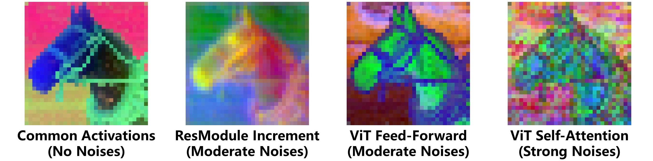
Figure 16: This visualization compares the high-frequency noises in various activations, showing three types of increment activations with strong noises.

E.2 Detailed In-Resolution Granularity Change

We have previously described the existence of in-resolution granularity changes, and this section will further detail the pattern of one such change. In one resolution of the up-stage, activations gradually shift from coarse to fine granularity, which aligns with intuition. However, the diffusion U-Net tends to overly refine the inter-module activations, resulting in slight noises in the last few inter-module activations due to excessive detail. This can be observed from the visualization of Figure 17. Consequently, a drop in discriminative performance is often seen near the end of one resolution.

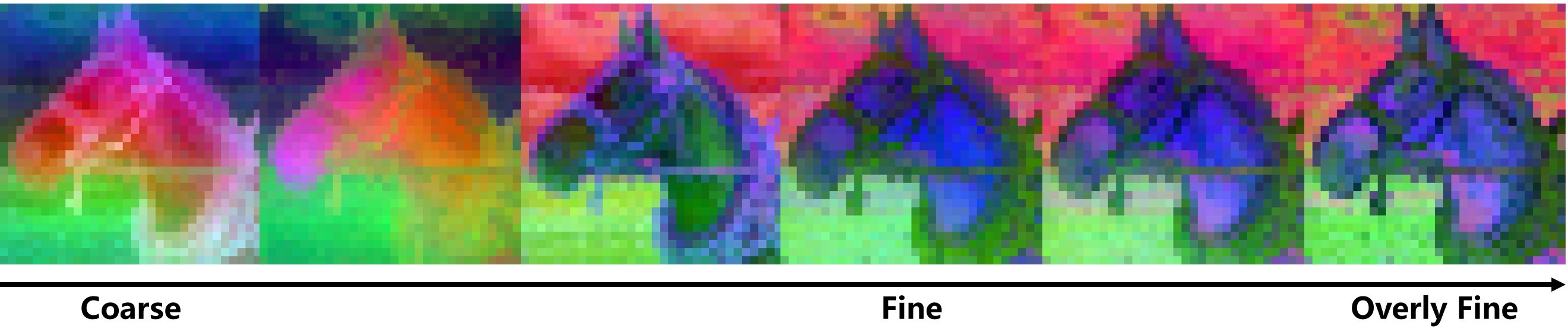
Figure 17: This visualization shows the granularity change across all inter-module activations of one resolution. At the end, the activations start to contain some slight noises, which is a sign of over-refinement.

E.3 Collaboration between Embedded ViTs

Multiple ViTs exist within one resolution; for example, one resolution in the up-stage typically contains three ViTs. These ViTs collaborate in refining the main inter-module residual. During this process, each ViT exhibits an inner granularity change as it produces the increment activation, and the changes of collaborating ViTs form a certain pattern. To be specific, the change of one ViT overlaps with the previous one to some extent but also shifts as a whole towards finer granularity, which is shown in Figure 18.

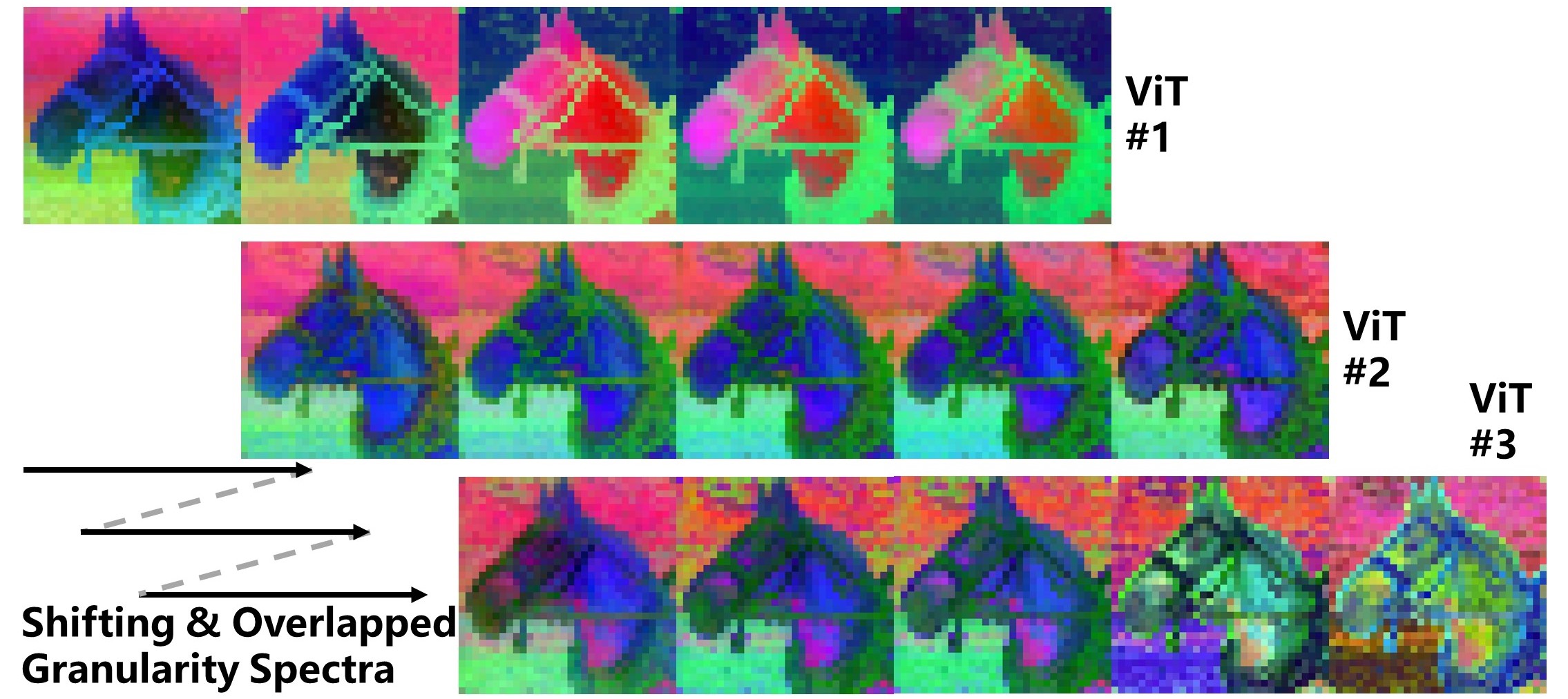
Figure 18: This visualization shows that the collaborating ViTs within one resolution contain overlapped and shifting granularity changes.

Appendix F Future Direction

It might be a good future direction to focus on more challenging discrimination scenarios. Specifically, long tail and out-of-distribution are important problems in discrimination, which can greatly hinder the performance of models that work well under i.i.d. settings [49]. There have been a few attempts to address this more challenging problem with diffusion models. For example, the disentanglement property of prompts might grant diffusion features cross-domain capability [16]. It is also possible to utilize diffusion models to synthesize training samples to adjust training data distribution [50, 55]. Given these attempts, more efforts are still required to be put in this direction. Moreover, there is a recent study [17] that might boost long tail and out-of-distribution discrimination using diffusion models. To be specific, AUC is an evaluation metric as well as a loss function that promotes good performance on both head and tail samples, which is an important tool for long tail and out-of-distribution studies [47, 48]. Conventionally, AUC is applicable to image classification but not semantic segmentation and other pixel-level tasks, but the aforementioned study manages to adopt AUC for semantic segmentation. Given this new tool, it is now made more viable to attempt to enhance diffusion feature on long tail and out-of-distribution problems.

Appendix G Computation Resources

We use Nvidia(R) RTX 3090 and Nvidia(R) RTX 4090 GPUs for the experiments, all with 24GB VRAM. Most of our experiments, except label-scarce segmentation, require no additional storage besides the necessary space for model checkpoints and datasets. The label-scarce segmentation task first extracts features and stores them on the disk, and then loads them for the downstream task, which takes about 4GB.

The codes are designed to be able to run on a single GPU or less than 4 GPUs, while multiple experiments can run simultaneously if more GPUs are provided. Each experiment on the semantic correspondence task takes about 5 hours. Each experiment on the large-scale semantic segmentation task takes 2 to 3 days, depending on the dataset. Each experiment on the label-scarce segmentation task takes about 1 hour, but we repeat on 5 random splits following [2], which increases the overall time. All the experiments in sum can be done within two weeks.

Our quantitative comparison is based on the label-scarce segmentation task, each run taking about 40 minutes. The time is shorter because the quantitative comparison evaluates each activation individually. This comparison uses large storage, which is about 45GB per model per dataset. With the help of qualitative filtering, we can finish the quantitative comparison of one model on one dataset within 2 days.

Appendix H Asset License

• SPair-71k: Available at https://cvlab.postech.ac.kr/research/SPair-71k/.

• Label-scarce segmentation datasets (sourced from LSUN): Available at https://github.com/fyu/lsun.

• ADE20K: Custom (research-only, non-commercial), at https://groups.csail.mit.edu/vision/datasets/ADE20K/terms/.

• CityScapes: Custom, at https://www.cityscapes-dataset.com/license/.

NeurIPS Paper Checklist

1. Claims

2. Question: Do the main claims made in the abstract and introduction accurately reflect the paper’s contributions and scope?

3. Answer: [Yes]

4. Justification: We clearly state our contributions in the abstract and introduction.

5. Guidelines:

   • The answer NA means that the abstract and introduction do not include the claims made in the paper.

   • The abstract and/or introduction should clearly state the claims made, including the contributions made in the paper and important assumptions and limitations. A No or NA answer to this question will not be perceived well by the reviewers.

   • The claims made should match theoretical and experimental results, and reflect how much the results can be expected to generalize to other settings.

   • It is fine to include aspirational goals as motivation as long as it is clear that these goals are not attained by the paper.

6. Limitations

7. Question: Does the paper discuss the limitations of the work performed by the authors?

8. Answer: [Yes]

9. Justification: We discuss the limitations in Section 7, which are mainly related to DiT models [35].

10. Guidelines:

    • The answer NA means that the paper has no limitation while the answer No means that the paper has limitations, but those are not discussed in the paper.

    • The authors are encouraged to create a separate "Limitations" section in their paper.

    • The paper should point out any strong assumptions and how robust the results are to violations of these assumptions (e.g., independence assumptions, noiseless settings, model well-specification, asymptotic approximations only holding locally). The authors should reflect on how these assumptions might be violated in practice and what the implications would be.

    • The authors should reflect on the scope of the claims made, e.g., if the approach was only tested on a few datasets or with a few runs. In general, empirical results often depend on implicit assumptions, which should be articulated.

    • The authors should reflect on the factors that influence the performance of the approach. For example, a facial recognition algorithm may perform poorly when image resolution is low or images are taken in low lighting. Or a speech-to-text system might not be used reliably to provide closed captions for online lectures because it fails to handle technical jargon.

    • The authors should discuss the computational efficiency of the proposed algorithms and how they scale with dataset size.

    • If applicable, the authors should discuss possible limitations of their approach to address problems of privacy and fairness.

    • While the authors might fear that complete honesty about limitations might be used by reviewers as grounds for rejection, a worse outcome might be that reviewers discover limitations that aren’t acknowledged in the paper. The authors should use their best judgment and recognize that individual actions in favor of transparency play an important role in developing norms that preserve the integrity of the community. Reviewers will be specifically instructed to not penalize honesty concerning limitations.

11. Theory Assumptions and Proofs

12. Question: For each theoretical result, does the paper provide the full set of assumptions and a complete (and correct) proof?

13. Answer: [N/A]

14. Justification: We do not make theoretical contributions.

15. Guidelines:

    • The answer NA means that the paper does not include theoretical results.

    • All the theorems, formulas, and proofs in the paper should be numbered and cross-referenced.

    • All assumptions should be clearly stated or referenced in the statement of any theorems.

    • The proofs can either appear in the main paper or the supplemental material, but if they appear in the supplemental material, the authors are encouraged to provide a short proof sketch to provide intuition.

    • Inversely, any informal proof provided in the core of the paper should be complemented by formal proofs provided in appendix or supplemental material.

    • Theorems and Lemmas that the proof relies upon should be properly referenced.

16. Experimental Result Reproducibility

17. Question: Does the paper fully disclose all the information needed to reproduce the main experimental results of the paper to the extent that it affects the main claims and/or conclusions of the paper (regardless of whether the code and data are provided or not)?

18. Answer: [Yes]

19. Justification: The most important information to reproduce our results is the exact activations we select as features, and it is detailed in Appendix B.

20. Guidelines:

    • The answer NA means that the paper does not include experiments.

    • If the paper includes experiments, a No answer to this question will not be perceived well by the reviewers: Making the paper reproducible is important, regardless of whether the code and data are provided or not.

    • If the contribution is a dataset and/or model, the authors should describe the steps taken to make their results reproducible or verifiable.

    • Depending on the contribution, reproducibility can be accomplished in various ways. For example, if the contribution is a novel architecture, describing the architecture fully might suffice, or if the contribution is a specific model and empirical evaluation, it may be necessary to either make it possible for others to replicate the model with the same dataset, or provide access to the model. In general. releasing code and data is often one good way to accomplish this, but reproducibility can also be provided via detailed instructions for how to replicate the results, access to a hosted model (e.g., in the case of a large language model), releasing of a model checkpoint, or other means that are appropriate to the research performed.

    • While NeurIPS does not require releasing code, the conference does require all submissions to provide some reasonable avenue for reproducibility, which may depend on the nature of the contribution. For example

      1. If the contribution is primarily a new algorithm, the paper should make it clear how to reproduce that algorithm.

      2. If the contribution is primarily a new model architecture, the paper should describe the architecture clearly and fully.

      3. If the contribution is a new model (e.g., a large language model), then there should either be a way to access this model for reproducing the results or a way to reproduce the model (e.g., with an open-source dataset or instructions for how to construct the dataset).

      4. We recognize that reproducibility may be tricky in some cases, in which case authors are welcome to describe the particular way they provide for reproducibility. In the case of closed-source models, it may be that access to the model is limited in some way (e.g., to registered users), but it should be possible for other researchers to have some path to reproducing or verifying the results.

21. Open access to data and code

22. Question: Does the paper provide open access to the data and code, with sufficient instructions to faithfully reproduce the main experimental results, as described in supplemental material?

23. Answer: [No]

24. Justification: We will release the codes after acceptance. Besides, we have provided the necessary information for reproducing the experiments in this manuscript.

25. Guidelines:

    • The answer NA means that paper does not include experiments requiring code.

    • Please see the NeurIPS code and data submission guidelines (https://nips.cc/public/guides/CodeSubmissionPolicy) for more details.

    • While we encourage the release of code and data, we understand that this might not be possible, so “No” is an acceptable answer. Papers cannot be rejected simply for not including code, unless this is central to the contribution (e.g., for a new open-source benchmark).

    • The instructions should contain the exact command and environment needed to run to reproduce the results. See the NeurIPS code and data submission guidelines (https://nips.cc/public/guides/CodeSubmissionPolicy) for more details.

    • The authors should provide instructions on data access and preparation, including how to access the raw data, preprocessed data, intermediate data, and generated data, etc.

    • The authors should provide scripts to reproduce all experimental results for the new proposed method and baselines. If only a subset of experiments are reproducible, they should state which ones are omitted from the script and why.

    • At submission time, to preserve anonymity, the authors should release anonymized versions (if applicable).

    • Providing as much information as possible in supplemental material (appended to the paper) is recommended, but including URLs to data and code is permitted.

26. Experimental Setting/Details

27. Question: Does the paper specify all the training and test details (e.g., data splits, hyperparameters, how they were chosen, type of optimizer, etc.) necessary to understand the results?

28. Answer: [Yes]

29. Justification: We have included the experimental details in Appendix C.

30. Guidelines:

    • The answer NA means that the paper does not include experiments.

    • The experimental setting should be presented in the core of the paper to a level of detail that is necessary to appreciate the results and make sense of them.

    • The full details can be provided either with the code, in appendix, or as supplemental material.

31. Experiment Statistical Significance

32. Question: Does the paper report error bars suitably and correctly defined or other appropriate information about the statistical significance of the experiments?

33. Answer: [Yes]

34. Justification: We provide error bars for some experimental results. Others are omitted as it can too computationally expensive, such as about two days per run.

35. Guidelines:

    • The answer NA means that the paper does not include experiments.

    • The authors should answer "Yes" if the results are accompanied by error bars, confidence intervals, or statistical significance tests, at least for the experiments that support the main claims of the paper.

    • The factors of variability that the error bars are capturing should be clearly stated (for example, train/test split, initialization, random drawing of some parameter, or overall run with given experimental conditions).

    • The method for calculating the error bars should be explained (closed form formula, call to a library function, bootstrap, etc.)

    • The assumptions made should be given (e.g., Normally distributed errors).

    • It should be clear whether the error bar is the standard deviation or the standard error of the mean.

    • It is OK to report 1-sigma error bars, but one should state it. The authors should preferably report a 2-sigma error bar than state that they have a 96% CI, if the hypothesis of Normality of errors is not verified.

    • For asymmetric distributions, the authors should be careful not to show in tables or figures symmetric error bars that would yield results that are out of range (e.g. negative error rates).

    • If error bars are reported in tables or plots, The authors should explain in the text how they were calculated and reference the corresponding figures or tables in the text.

36. Experiments Compute Resources

37. Question: For each experiment, does the paper provide sufficient information on the computer resources (type of compute workers, memory, time of execution) needed to reproduce the experiments?

38. Answer: [Yes]

39. Justification: We provide information in Appendix G.

40. Guidelines:

    • The answer NA means that the paper does not include experiments.

    • The paper should indicate the type of compute workers CPU or GPU, internal cluster, or cloud provider, including relevant memory and storage.

    • The paper should provide the amount of compute required for each of the individual experimental runs as well as estimate the total compute.

    • The paper should disclose whether the full research project required more compute than the experiments reported in the paper (e.g., preliminary or failed experiments that didn’t make it into the paper).

41. Code Of Ethics

42. Question: Does the research conducted in the paper conform, in every respect, with the NeurIPS Code of Ethics https://neurips.cc/public/EthicsGuidelines?

43. Answer: [Yes]

44. Justification: We conform with the NeurIPS Code of Ethics.

45. Guidelines:

    • The answer NA means that the authors have not reviewed the NeurIPS Code of Ethics.

    • If the authors answer No, they should explain the special circumstances that require a deviation from the Code of Ethics.

    • The authors should make sure to preserve anonymity (e.g., if there is a special consideration due to laws or regulations in their jurisdiction).

46. Broader Impacts

47. Question: Does the paper discuss both potential positive societal impacts and negative societal impacts of the work performed?

48. Answer: [N/A]

49. Justification: There is no socetal impact.

50. Guidelines:

    • The answer NA means that there is no societal impact of the work performed.

    • If the authors answer NA or No, they should explain why their work has no societal impact or why the paper does not address societal impact.

    • Examples of negative societal impacts include potential malicious or unintended uses (e.g., disinformation, generating fake profiles, surveillance), fairness considerations (e.g., deployment of technologies that could make decisions that unfairly impact specific groups), privacy considerations, and security considerations.

    • The conference expects that many papers will be foundational research and not tied to particular applications, let alone deployments. However, if there is a direct path to any negative applications, the authors should point it out. For example, it is legitimate to point out that an improvement in the quality of generative models could be used to generate deepfakes for disinformation. On the other hand, it is not needed to point out that a generic algorithm for optimizing neural networks could enable people to train models that generate Deepfakes faster.

    • The authors should consider possible harms that could arise when the technology is being used as intended and functioning correctly, harms that could arise when the technology is being used as intended but gives incorrect results, and harms following from (intentional or unintentional) misuse of the technology.

    • If there are negative societal impacts, the authors could also discuss possible mitigation strategies (e.g., gated release of models, providing defenses in addition to attacks, mechanisms for monitoring misuse, mechanisms to monitor how a system learns from feedback over time, improving the efficiency and accessibility of ML).

51. Safeguards

52. Question: Does the paper describe safeguards that have been put in place for responsible release of data or models that have a high risk for misuse (e.g., pretrained language models, image generators, or scraped datasets)?

53. Answer: [N/A]

54. Justification: The paper poses no such risks.

55. Guidelines:

    • The answer NA means that the paper poses no such risks.

    • Released models that have a high risk for misuse or dual-use should be released with necessary safeguards to allow for controlled use of the model, for example by requiring that users adhere to usage guidelines or restrictions to access the model or implementing safety filters.

    • Datasets that have been scraped from the Internet could pose safety risks. The authors should describe how they avoided releasing unsafe images.

    • We recognize that providing effective safeguards is challenging, and many papers do not require this, but we encourage authors to take this into account and make a best faith effort.

56. Licenses for existing assets

57. Question: Are the creators or original owners of assets (e.g., code, data, models), used in the paper, properly credited and are the license and terms of use explicitly mentioned and properly respected?

58. Answer: [Yes]

59. Justification: We cite the original papers where related assets are first mentioned and list their license in Appendix H.

60. Guidelines:

    • The answer NA means that the paper does not use existing assets.

    • The authors should cite the original paper that produced the code package or dataset.

    • The authors should state which version of the asset is used and, if possible, include a URL.

    • The name of the license (e.g., CC-BY 4.0) should be included for each asset.

    • For scraped data from a particular source (e.g., website), the copyright and terms of service of that source should be provided.

    • If assets are released, the license, copyright information, and terms of use in the package should be provided. For popular datasets, paperswithcode.com/datasets has curated licenses for some datasets. Their licensing guide can help determine the license of a dataset.

    • For existing datasets that are re-packaged, both the original license and the license of the derived asset (if it has changed) should be provided.

    • If this information is not available online, the authors are encouraged to reach out to the asset’s creators.

61. New Assets

62. Question: Are new assets introduced in the paper well documented and is the documentation provided alongside the assets?

63. Answer: [N/A]

64. Justification: We do not introduce new assets.

65. Guidelines:

    • The answer NA means that the paper does not release new assets.

    • Researchers should communicate the details of the dataset/code/model as part of their submissions via structured templates. This includes details about training, license, limitations, etc.

    • The paper should discuss whether and how consent was obtained from people whose asset is used.

    • At submission time, remember to anonymize your assets (if applicable). You can either create an anonymized URL or include an anonymized zip file.

66. Crowdsourcing and Research with Human Subjects

67. Question: For crowdsourcing experiments and research with human subjects, does the paper include the full text of instructions given to participants and screenshots, if applicable, as well as details about compensation (if any)?

68. Answer: [N/A]

69. Justification: The paper does not involve crowdsourcing nor research with human subjects.

70. Guidelines:

    • The answer NA means that the paper does not involve crowdsourcing nor research with human subjects.

    • Including this information in the supplemental material is fine, but if the main contribution of the paper involves human subjects, then as much detail as possible should be included in the main paper.

    • According to the NeurIPS Code of Ethics, workers involved in data collection, curation, or other labor should be paid at least the minimum wage in the country of the data collector.

71. Institutional Review Board (IRB) Approvals or Equivalent for Research with Human Subjects

72. Question: Does the paper describe potential risks incurred by study participants, whether such risks were disclosed to the subjects, and whether Institutional Review Board (IRB) approvals (or an equivalent approval/review based on the requirements of your country or institution) were obtained?

73. Answer: [N/A]

74. Justification: The paper does not involve human subjects.

75. Guidelines:

    • The answer NA means that the paper does not involve crowdsourcing nor research with human subjects.

    • Depending on the country in which research is conducted, IRB approval (or equivalent) may be required for any human subjects research. If you obtained IRB approval, you should clearly state this in the paper.

    • We recognize that the procedures for this may vary significantly between institutions and locations, and we expect authors to adhere to the NeurIPS Code of Ethics and the guidelines for their institution.

    • For initial submissions, do not include any information that would break anonymity (if applicable), such as the institution conducting the review.

References

- [1] Shir Amir, Yossi Gandelsman, Shai Bagon, and Tali Dekel. Deep vit features as dense visual descriptors. ECCV Workshop on What is Motion For, 2022.
- [2] Dmitry Baranchuk, Andrey Voynov, Ivan Rubachev, Valentin Khrulkov, and Artem Babenko. Label-efficient semantic segmentation with diffusion models. In The Tenth International Conference on Learning Representations, 2022.
- [3] Mathilde Caron, Ishan Misra, Julien Mairal, Priya Goyal, Piotr Bojanowski, and Armand Joulin. Unsupervised learning of visual features by contrasting cluster assignments. In Annual Conference on Neural Information Processing Systems, 2020.
- [4] Mathilde Caron, Hugo Touvron, Ishan Misra, Hervé Jégou, Julien Mairal, Piotr Bojanowski, and Armand Joulin. Emerging properties in self-supervised vision transformers. In IEEE/CVF International Conference on Computer Vision, ICCV, pages 9630–9640, 2021.
- [5] Shan Carter, Zan Armstrong, Ludwig Schubert, Ian Johnson, and Chris Olah. Activation atlas. Distill, 4(3):e15, 2019.
- [6] Haoxin Chen, Yong Zhang, Xiaodong Cun, Menghan Xia, Xintao Wang, Chao Weng, and Ying Shan. Videocrafter2: Overcoming data limitations for high-quality video diffusion models. CoRR, abs/2401.09047, 2024.
- [7] Huanran Chen, Yinpeng Dong, Shitong Shao, Zhongkai Hao, Xiao Yang, Hang Su, and Jun Zhu. Your diffusion model is secretly a certifiably robust classifier. CoRR, abs/2402.02316, 2024.
- [8] Marius Cordts, Mohamed Omran, Sebastian Ramos, Timo Rehfeld, Markus Enzweiler, Rodrigo Benenson, Uwe Franke, Stefan Roth, and Bernt Schiele. The cityscapes dataset for semantic urban scene understanding. In IEEE Conference on Computer Vision and Pattern Recognition, pages 3213–3223, 2016.
- [9] Jia Deng, Wei Dong, Richard Socher, Li-Jia Li, Kai Li, and Li Fei-Fei. Imagenet: A large-scale hierarchical image database. In IEEE Computer Society Conference on Computer Vision and Pattern Recognition, pages 248–255, 2009.
- [10] Prafulla Dhariwal and Alexander Quinn Nichol. Diffusion models beat gans on image synthesis. In Annual Conference on Neural Information Processing Systems, pages 8780–8794, 2021.
- [11] Zheng Ding, Jieke Wang, and Zhuowen Tu. Open-vocabulary universal image segmentation with maskclip. In International Conference on Machine Learning, ICML, volume 202 of Proceedings of Machine Learning Research, pages 8090–8102, 2023.
- [12] Alexey Dosovitskiy, Lucas Beyer, Alexander Kolesnikov, Dirk Weissenborn, Xiaohua Zhai, Thomas Unterthiner, Mostafa Dehghani, Matthias Minderer, Georg Heigold, Sylvain Gelly, Jakob Uszkoreit, and Neil Houlsby. An image is worth 16x16 words: Transformers for image recognition at scale. In 9th International Conference on Learning Representations, 2021.
- [13] Niladri Shekhar Dutt, Sanjeev Muralikrishnan, and Niloy J. Mitra. Diffusion 3d features (diff3f) decorating untextured shapes with distilled semantic features. In IEEE/CVF Conference on Computer Vision and Pattern Recognition, pages 4494–4504, 2024.
- [14] Raphael Antonius Frick and Martin Steinebach. Diffseg: Towards detecting diffusion-based inpainting attacks using multi-feature segmentation. In IEEE/CVF Conference on Computer Vision and Pattern Recognition, pages 3802–3808, 2024.
- [15] Mor Geva, Roei Schuster, Jonathan Berant, and Omer Levy. Transformer feed-forward layers are key-value memories. In Proceedings of the 2021 Conference on Empirical Methods in Natural Language Processing, pages 5484–5495, 2021.
- [16] Rui Gong, Martin Danelljan, Han Sun, Julio Delgado Mangas, and Luc Van Gool. Prompting diffusion representations for cross-domain semantic segmentation. CoRR, abs/2307.02138, 2023.
- [17] Boyu Han, Qianqian Xu, Zhiyong Yang, Shilong Bao, Peisong Wen, Yangbangyan Jiang, and Qingming Huang. Aucseg: Auc-oriented pixel-level long-tail semantic segmentation, 2024.
- [18] Shijie Hao, Yuan Zhou, and Yanrong Guo. A brief survey on semantic segmentation with deep learning. Neurocomputing, 406:302–321, 2020.
- [19] Kaiming He, Xinlei Chen, Saining Xie, Yanghao Li, Piotr Dollár, and Ross B. Girshick. Masked autoencoders are scalable vision learners. In IEEE/CVF Conference on Computer Vision and Pattern Recognition, pages 15979–15988, 2022.
- [20] Kaiming He, Xiangyu Zhang, Shaoqing Ren, and Jian Sun. Deep residual learning for image recognition. In IEEE Conference on Computer Vision and Pattern Recognition, pages 770–778, 2016.
- [21] Jonathan Ho, Ajay Jain, and Pieter Abbeel. Denoising diffusion probabilistic models. In Annual Conference on Neural Information Processing Systems, 2020.
- [22] Yuanfeng Ji, Zhe Chen, Enze Xie, Lanqing Hong, Xihui Liu, Zhaoqiang Liu, Tong Lu, Zhenguo Li, and Ping Luo. DDP: diffusion model for dense visual prediction. In IEEE/CVF International Conference on Computer Vision, pages 21684–21695, 2023.
- [23] Bingxin Ke, Anton Obukhov, Shengyu Huang, Nando Metzger, Rodrigo Caye Daudt, and Konrad Schindler. Repurposing diffusion-based image generators for monocular depth estimation. CoRR, abs/2312.02145, 2023.
- [24] Neehar Kondapaneni, Markus Marks, Manuel Knott, Rogério Guimarães, and Pietro Perona. Text-image alignment for diffusion-based perception. CoRR, abs/2310.00031, 2023.
- [25] Alex Krizhevsky, Geoffrey Hinton, et al. Learning multiple layers of features from tiny images. 2009.
- [26] Alexander C. Li, Mihir Prabhudesai, Shivam Duggal, Ellis Brown, and Deepak Pathak. Your diffusion model is secretly a zero-shot classifier. In IEEE/CVF International Conference on Computer Vision, pages 2206–2217, 2023.
- [27] Xinghui Li, Jingyi Lu, Kai Han, and Victor Prisacariu. Sd4match: Learning to prompt stable diffusion model for semantic matching. CoRR, abs/2310.17569, 2023.
- [28] Yaron Lipman, Ricky T. Q. Chen, Heli Ben-Hamu, Maximilian Nickel, and Matthew Le. Flow matching for generative modeling. In The Eleventh International Conference on Learning Representations, 2023.
- [29] Grace Luo, Lisa Dunlap, Dong Huk Park, Aleksander Holynski, and Trevor Darrell. Diffusion hyperfeatures: Searching through time and space for semantic correspondence. In Annual Conference on Neural Information Processing Systems, 2023.
- [30] Juhong Min, Jongmin Lee, Jean Ponce, and Minsu Cho. Spair-71k: A large-scale benchmark for semantic correspondence. CoRR, abs/1908.10543, 2019.
- [31] Juhong Min, Jongmin Lee, Jean Ponce, and Minsu Cho. Learning to compose hypercolumns for visual correspondence. In Computer Vision - ECCV 2020 - 16th European Conference, volume 12360, pages 346–363. Springer, 2020.
- [32] Soumik Mukhopadhyay, Matthew Gwilliam, Vatsal Agarwal, Namitha Padmanabhan, Archana Swaminathan, Srinidhi Hegde, Tianyi Zhou, and Abhinav Shrivastava. Diffusion models beat gans on image classification. CoRR, abs/2307.08702, 2023.
- [33] Soumik Mukhopadhyay, Matthew Gwilliam, Yosuke Yamaguchi, Vatsal Agarwal, Namitha Padmanabhan, Archana Swaminathan, Tianyi Zhou, and Abhinav Shrivastava. Do text-free diffusion models learn discriminative visual representations? CoRR, abs/2311.17921, 2023.
- [34] Chris Olah, Alexander Mordvintsev, and Ludwig Schubert. Feature visualization. Distill, 2(11):e7, 2017.
- [35] William Peebles and Saining Xie. Scalable diffusion models with transformers. In IEEE/CVF International Conference on Computer Vision, pages 4172–4182, 2023.
- [36] Dustin Podell, Zion English, Kyle Lacey, Andreas Blattmann, Tim Dockhorn, Jonas Müller, Joe Penna, and Robin Rombach. SDXL: improving latent diffusion models for high-resolution image synthesis. CoRR, abs/2307.01952, 2023.
- [37] Robin Rombach, Andreas Blattmann, Dominik Lorenz, Patrick Esser, and Björn Ommer. High-resolution image synthesis with latent diffusion models. In IEEE/CVF Conference on Computer Vision and Pattern Recognition, pages 10674–10685, 2022.
- [38] Olaf Ronneberger, Philipp Fischer, and Thomas Brox. U-net: Convolutional networks for biomedical image segmentation. In Medical Image Computing and Computer-Assisted Intervention, volume 9351, pages 234–241. Springer, 2015.
- [39] Yang Song, Jascha Sohl-Dickstein, Diederik P. Kingma, Abhishek Kumar, Stefano Ermon, and Ben Poole. Score-based generative modeling through stochastic differential equations. In 9th International Conference on Learning Representations, 2021.
- [40] Xuan Su, Jiaming Song, Chenlin Meng, and Stefano Ermon. Dual diffusion implicit bridges for image-to-image translation. In The Eleventh International Conference on Learning Representations, 2023.
- [41] Luming Tang, Menglin Jia, Qianqian Wang, Cheng Perng Phoo, and Bharath Hariharan. Emergent correspondence from image diffusion. In Annual Conference on Neural Information Processing Systems, 2023.
- [42] Kashvi Taunk, Sanjukta De, Srishti Verma, and Aleena Swetapadma. A brief review of nearest neighbor algorithm for learning and classification. In 2019 international conference on intelligent computing and control systems (ICCS), pages 1255–1260. IEEE, 2019.
- [43] Junjiao Tian, Lavisha Aggarwal, Andrea Colaco, Zsolt Kira, and Mar González-Franco. Diffuse, attend, and segment: Unsupervised zero-shot segmentation using stable diffusion. CoRR, abs/2308.12469, 2023.
- [44] Ashish Vaswani, Noam Shazeer, Niki Parmar, Jakob Uszkoreit, Llion Jones, Aidan N. Gomez, Lukasz Kaiser, and Illia Polosukhin. Attention is all you need. In Annual Conference on Neural Information Processing Systems, pages 5998–6008, 2017.
- [45] Martina G. Vilas, Timothy Schaumlöffel, and Gemma Roig. Analyzing vision transformers for image classification in class embedding space. In Annual Conference on Neural Information Processing Systems 2023, 2023.
- [46] Qiang Wan, Zilong Huang, Bingyi Kang, Jiashi Feng, and Li Zhang. Harnessing diffusion models for visual perception with meta prompts. CoRR, abs/2312.14733, 2023.
- [47] Zitai Wang, Qianqian Xu, Zhiyong Yang, Yuan He, Xiaochun Cao, and Qingming Huang. Openauc: Towards auc-oriented open-set recognition. In Annual Conference on Neural Information Processing Systems, 2022.
- [48] Zitai Wang, Qianqian Xu, Zhiyong Yang, Yuan He, Xiaochun Cao, and Qingming Huang. Optimizing partial area under the top-k curve: Theory and practice. IEEE Trans. Pattern Anal. Mach. Intell., 45(4):5053–5069, 2023.
- [49] Zitai Wang, Qianqian Xu, Zhiyong Yang, Yuan He, Xiaochun Cao, and Qingming Huang. A unified generalization analysis of re-weighting and logit-adjustment for imbalanced learning. In Annual Conference on Neural Information Processing Systems, 2023.
- [50] Weijia Wu, Yuzhong Zhao, Hao Chen, Yuchao Gu, Rui Zhao, Yefei He, Hong Zhou, Mike Zheng Shou, and Chunhua Shen. Datasetdm: Synthesizing data with perception annotations using diffusion models. In Annual Conference on Neural Information Processing Systems, 2023.
- [51] Changming Xiao, Qi Yang, Feng Zhou, and Changshui Zhang. From text to mask: Localizing entities using the attention of text-to-image diffusion models. CoRR, abs/2309.04109, 2023.
- [52] Jiarui Xu, Sifei Liu, Arash Vahdat, Wonmin Byeon, Xiaolong Wang, and Shalini De Mello. Open-vocabulary panoptic segmentation with text-to-image diffusion models. In IEEE/CVF Conference on Computer Vision and Pattern Recognition, pages 2955–2966, 2023.
- [53] Xingyi Yang and Xinchao Wang. Diffusion model as representation learner. In IEEE/CVF International Conference on Computer Vision, pages 18892–18903, 2023.
- [54] Fisher Yu, Yinda Zhang, Shuran Song, Ari Seff, and Jianxiong Xiao. LSUN: construction of a large-scale image dataset using deep learning with humans in the loop. CoRR, abs/1506.03365, 2015.
- [55] David Junhao Zhang, Mutian Xu, Chuhui Xue, Wenqing Zhang, Xiaoguang Han, Song Bai, and Mike Zheng Shou. Free-atm: Exploring unsupervised learning on diffusion-generated images with free attention masks. CoRR, abs/2308.06739, 2023.
- [56] Junyi Zhang, Charles Herrmann, Junhwa Hur, Luisa Polania Cabrera, Varun Jampani, Deqing Sun, and Ming-Hsuan Yang. A tale of two features: Stable diffusion complements DINO for zero-shot semantic correspondence. In Annual Conference on Neural Information Processing Systems, 2023.
- [57] Zhengxin Zhang, Qingjie Liu, and Yunhong Wang. Road extraction by deep residual u-net. IEEE Geosci. Remote. Sens. Lett., 15(5):749–753, 2018.
- [58] Wenliang Zhao, Yongming Rao, Zuyan Liu, Benlin Liu, Jie Zhou, and Jiwen Lu. Unleashing text-to-image diffusion models for visual perception. In IEEE/CVF International Conference on Computer Vision, pages 5706–5716, 2023.
- [59] Bolei Zhou, Hang Zhao, Xavier Puig, Sanja Fidler, Adela Barriuso, and Antonio Torralba. Scene parsing through ADE20K dataset. In IEEE Conference on Computer Vision and Pattern Recognition, pages 5122–5130, 2017.
- [60] Jingyi Zhou, Jiamu Sheng, Jiayuan Fan, Peng Ye, Tong He, Bin Wang, and Tao Chen. When hyperspectral image classification meets diffusion models: An unsupervised feature learning framework. CoRR, abs/2306.08964, 2023.