First-order methods and automatic differentiation: A multi-step systems identification perspective

Abstract

This paper presents a tool for multi-step system identification that leverages first-order optimization and exact gradient computation. Drawing inspiration from neural network training and Automatic Differentiation (AD), the proposed method computes and analyzes the gradients with respect to the parameters to identify by propagating them through system dynamics. Thus, it defines a linear, time-varying dynamical system that models the gradient evolution. This allows to formally address the “exploding gradient” issue, by providing conditions for a reliable and efficient optimization and identification process for dynamical systems. Results indicate that the proposed method is both effective and efficient, making it a promising tool for future research and applications in nonlinear systems identification and non-convex optimization.

I Introduction

Over the past few decades, the field of nonlinear systems identification has received significant attention. Indeed, modern engineering applications are growingly requiring the development of sophisticated models, capable of delivering accurate estimates over extended time periods, highlighting the need for approaches that ensure the minimization of multi-step prediction errors. Clearly, the identification of such types of models may easily destroy nice convexity properties of the associated cost functions, thus leading to hard optimization problems.

In such a situation, first-order methods offer a practical and effective solution. Such methods, which under suitable conditions are guaranteed to converge to a solution (in general sub-optimal), have recently gained popularity for their ability to tackle large-scale and complex problems [1, 2]. First-order methods leverage gradient information to iteratively improve the solution [3], and their effectiveness in solving non-convex problems remains one of the unresolved mysteries contributing to the success of deep learning across numerous applications (see, e.g., [4] and references therein). Indeed, their ability to provide feasible solutions within reasonable computational effort, even in the absence of convexity, makes them an appealing choice for tackling the optimization challenges presented by complex identification problems.

The contribution of this work is to present a computable tool to leverage first-order methods, which have been at the core of the success of NN-based approaches, for solving optimization problems central to multi-step identification. In particular, we exploit the explicit knowledge of the physical dependencies characterizing the system to identify and propose an efficient method to compute the exact gradient and estimate system parameters. The method is inspired by the classical backpropagation scheme, adopted, e.g., in neural networks, and recently proposed in the context of system identification in our recent work [5], and similarly in [6]. Similarly to backpropagation-through-time [7], where the error is back-propagated in time in an unfolded Recurrent Neural Network (RNN) after forward-propagating the inputs through the unfolded network, we represent the evolution of the gradient by studying the predictions and errors of the system as they evolve forward-in-time, as typically done with the forward automatic differentiation [8]. Thus, we propagate the gradient through the recursion intrinsically defined in dynamical systems updating it while propagating the predicted states.

Certainly, various methods are available in the literature for calculating the gradient, with varying degrees of approximation, and, at least in principle, all of these can be applied, ranging from techniques based on numerical differentiation to generic automatic differentiation [8, 9]. Indeed, in the context of system identification, several works have explored the application of classical automatic differentiation to parameter estimation (see, e.g., [10, 11]). However, a more in-depth analysis of the application of automatic differentiation to multi-step identification problems and, in particular, to the framework we propose in [12] sheds light on several distinguishing characteristics that make it of particular interest. First, the method offers a “smart way” to evaluate the exact gradient when dealing with the identification of dynamical systems, significantly improving the computational performance compared to our previous work [5]. Second, it allows the definition of a particular linear, time-varying dynamical system describing the evolution of the gradient with respect to parameters and the initial condition, directly linked to the dynamics of the system we aim at identifying. Specifically, we will show in Section IV how it can be used to derive conditions for avoiding the so-called phenomenon of the “exploding gradient”, which involves a gradient stability study. Indeed, model predictions may exhibit finite escape time phenomena for certain parameters or initial condition values, leading to explosive behavior and consequent exploding gradients. This behavior might hinder the optimization process and, consequently, the identification.

This motivates the use of penalties, such as barrier functions on the states and parameters, to avoid this issue during the training and force the estimated parameters to generate trajectories that are bounded in finite time. Consequently, it allows the training process to remain in a “safe” neighborhood around the measured trajectory, ensuring that the optimization process remains consistent and reliable.

The paper is structured as follows. In Section II, the identification framework presented in [12] is summarized and multi-step identification problems are discussed. Then, the dynamical system describing the evolution of the gradient is detailed in Section III, and in Section III-B an Algorithm describing the proposed approach is presented and discussed together with the computational complexity of the proposed approach. In Section IV the stability of the gradient is analyzed, deriving sufficient conditions for avoiding exploding gradients. Numerical results are discussed in Section V, while main conclusions and future research directions are drawn in Section VI.

Notation Given integers ${a,b\in\mathbb{N}}$, ${a\leq b}$, we denote by $[a,b]$ the set of integers $\{a,\ldots,b\}$.

II Preliminaries

II-A Problem setup

In this section, we outline the considered multi-step system identification problem, recalling the framework presented and deeply analyzed in [12].

We consider a nonlinear, time-invariant system described by the following mathematical model

$$\mathcal{S}: x_{k+1}=f\left({x}_{k},{u}_{k};\theta\right)+\Delta(x_{k},u_{k}),$$ (1)

$$z_{k}=h\left(x_{k}\right),$$

where $x\in\mathbb{R}^{n_{x}}$ is the state vector, $\theta\in\mathbb{R}^{n_{\theta}}$ is the parameter vector, $u\in\mathbb{R}^{n_{u}}$ is the input, and $z\in\mathbb{R}^{n_{z}}$ is the output. The functions $f$ and $h$ are known, representing part of the state update and observation functions, respectively. These functions are nonlinear, time-invariant, and continuously differentiable. The term $\Delta$, representing unmodeled dynamics, is unknown.

Given a multi-step input sequence and corresponding observations

$$\widetilde{\mathbf{u}}_{0:T} =\{\widetilde{u}_{0},\dots,\widetilde{u}_{T}\}, \widetilde{u}_{k}=u_{k}+\eta^{u}_{k},$$ (2)

$$\widetilde{\mathbf{z}}_{0:T} =\{\widetilde{z}_{0},\dots,\widetilde{z}_{T}\}, \widetilde{z}_{k}=z_{k}+\eta^{z}_{k},$$

with $\eta^{u}_{k}$ and $\eta^{z}_{k}$ representing the input and output measurement noise, we seek to estimate the unknown system parameters $\theta$, and initial conditions $x_{0}$, while compensating for the unknown term $\Delta$. To this aim, we define an estimation model $\mathcal{M}$ to approximate the system $\mathcal{S}$, i.e.,

$${\mathcal{M}}\,:\quad\widehat{x}_{k+1} ={f}(\widehat{x}_{k},{u}_{k};\widehat{\theta})+{\delta}(\widehat{x}_{k},u_{k};\omega),$$ (3)

$$\widehat{{z}}_{k} ={h}(\widehat{x}_{k};\widehat{\theta}),$$

where $\delta$ is a generic approximator (e.g., a linear combination of basis functions from a given dictionary) with design parameters $\omega$ to be learned.

In the proposed framework, the multi-step cost function takes the form

$$\mathcal{C}_{T}(\theta,x_{0},\omega;\mathbf{e}_{0:T},\widehat{\mathbf{x}}_{1:T})$$ (4)

$$\doteq\sum_{k=0}^{T}\left(\mathcal{L}_{k}\left(\theta,x_{0};e_{k}\right)+\lambda p(\widehat{x}_{k},\theta)+\nu q^{2}(\widehat{x}_{k},\theta)+{\gamma}r(\omega)\right),$$

where $\mathcal{L}_{k}$ is a general loss function depending on the prediction error $e_{k}=\widetilde{z}_{k}-\widehat{z}_{k}$, while $p,q$ and $r$ impose physical constraints [12, 13], and regularization of the black-box weights $\omega$, and $\lambda,\nu,\gamma\in\mathbb{R}$ are tunable coefficients. Here, $\mathcal{L}_{k}$, $p$, $q$, $r$ are assumed to be twice continuously differentiable functions.

The final goal is to estimate the optimal values of $\theta$, $x_{0}$, and $\omega$ by solving the following optimization problem

$$\left({\theta}^{\star},x_{0}^{\star},\omega^{\star}\right)\doteq\arg\min_{\theta,x_{0},\omega}\,\,\mathcal{C}_{T}.$$ (5)

The interested reader is referred to [12] for additional details on the framework.

II-B Multi-step identification

Multi-step identification involves minimizing a multi-step cost function over a horizon $T$, propagating the predictions ${\widehat{x}_{k}}$ over the desired horizon, and recursively applying the dynamical model $\mathcal{M}$. An approach somehow similar is found in RNNs [14], which aim at accurately estimating an output sequence by minimizing the sum-of-squares error measure over a finite horizon, involving the recursion of the hidden states repeatedly through the same layer. This implies that the network weights, as well as the architectures, are the same over the entire horizon. Thus, recalling the typical structure of neural networks, it is possible to represent the multi-step propagation of the model in (3) as in Fig. 1, drawing a parallelism between RNN layers and dynamics propagation of the model (3).

Figure 1: Multi-step model propagation.

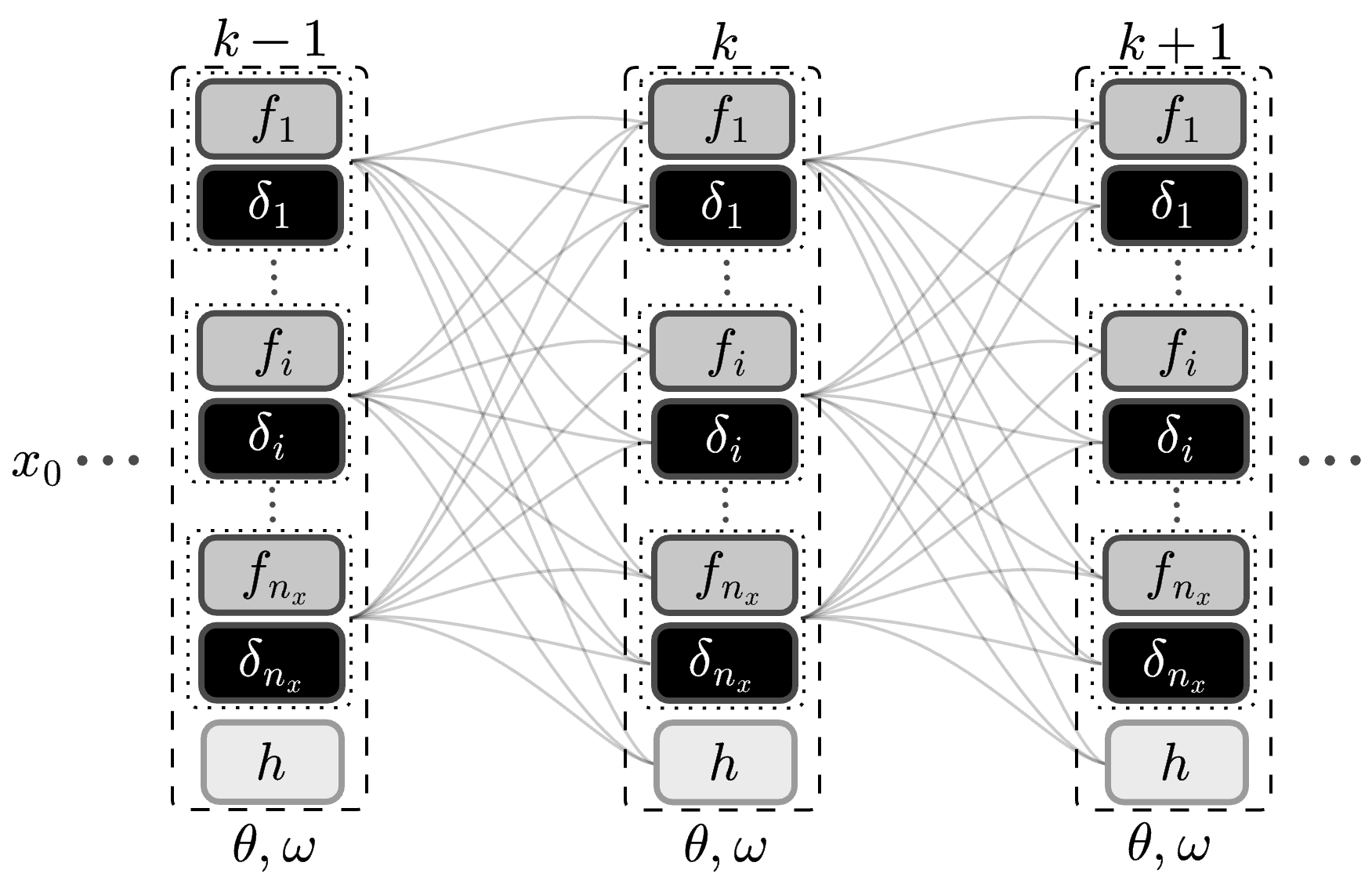
Similarly to RNN, during the identification process, we need to consider the same weights, i.e., parameters to identify, and the same structure, i.e., functional form of the model, to be the same at each time step along the prediction horizon $T$, in order to preserve physical consistency and temporal dependencies in the learning process. This similarity led us to investigate techniques commonly used for optimizing recurrent neural networks, such as backpropagation through time [5, 7], and, more in general, automatic differentiation, in the context of multi-step system identification.

In the next section, we focus on analyzing how the gradient may be efficiently evaluated in multi-step identification problems. In particular, we will show that by exploiting automatic differentiation it is possible to define a specific linear, time-varying (LTV) dynamical system that models the gradient evolution along the multi-step horizon for the structure depicted in Fig. 1, that is very general and can be used for the identification of every dynamical system. Thus, a (possibly local) solution for the optimization problem (5) can be obtained through first-order methods.

III Automatic differentiation in multi-step system identification

At the core of first-order techniques is the computation of the gradient of the cost function $\mathcal{C}_{T}$ evaluated at the current solution. For instance, in standard gradient descent, once the gradients with respect to the parameter $\nabla_{\theta}\mathcal{C}_{T}\in\mathbb{R}^{n_{\theta}}$, and the initial condition $\nabla_{x_{0}}\mathcal{C}_{T}\in\mathbb{R}^{n_{x}}$ are computed, the weights are updated in the direction that minimizes the total cost, i.e.,

$$\widehat{\theta}\leftarrow\widehat{\theta}-\varsigma_{\theta}\nabla_{\theta}\mathcal{C}_{T},\quad\widehat{x}_{0}\leftarrow\widehat{x}_{0}-\varsigma_{x_{0}}\nabla_{x_{0}}\mathcal{C}_{T},$$ (6)

where $\varsigma_{\theta}$ and $\varsigma_{x_{0}}$ are the learning rates, that can be designed exploiting state-of-the-art methods [15].

In this context, automatic differentiation is a general computational technique used to efficiently compute the gradients of functions, often applied in optimization and machine learning. It relies on the concept of graph computation, where a function is decomposed into a series of elementary operations, each represented as a node in a computational graph. The edges of this graph represent the flow of data between operations. Thus, AD systematically applies the chain rule of calculus to propagate derivatives through this graph. By evaluating both the function and its derivatives simultaneously, AD avoids numerical errors typically associated with finite difference methods and is computationally more efficient than symbolic differentiation [8]. In the context of multi-step identification of dynamical systems, the computational graph becomes very specialized due to the recursive nature of the problem. This recursive structure allows for efficient gradient evaluation at each time step, effectively turning the gradient evolution into a dynamical system itself, directly connected to the estimation model (3), exploited to identify the system under analysis. Indeed, state equations of dynamical systems exhibit a highly specific structure that can be leveraged for AD, making the process both general and well-suited for system identification. Specifically, unlike traditional AD applications, we do not need to explicitly capture all dependencies, enabling smarter optimization processes in multi-step system identification that, despite AD typically complex structure, reveals a recursive efficiency valid for any dynamical system.

In this section, we exploit the explicit knowledge of the structure of the dynamical system (1) and the defined estimation model (3), and present a novel and efficient adaptation of the forward automatic differentiation technique to the context of system identification.

III-A Gradient dynamics

Before presenting our first result, we introduce some additional simplifying notation: the Jacobian matrices of $e_{k}$ with respect to $z_{k}$ and of $z_{k}$ with respect to $x_{k}$ are denoted as  $\mathcal{J}^{e\!/\!z}_{k}\doteq\frac{\partial e_{k}}{\partial z_{k}}\in\mathbb{R}^{n_{z},n_{z}}$, and $\mathcal{J}^{z\!/\!x}_{k}\doteq\frac{\partial z_{k}}{\partial x_{k}}\in\mathbb{R}^{n_{z},n_{x}}$, respectively. Similarly, $\mathcal{J}^{x\!/\!\theta}_{k}\doteq\frac{\partial x_{k}}{\partial\theta}\in\mathbb{R}^{n_{x},n_{\theta}}$ is the Jacobian matrix of $x_{k}$ with respect to $\theta$, while $\mathcal{J}^{x\!/\!x}_{k}\doteq\frac{\partial x_{k}}{\partial x_{k-1}}\in\mathbb{R}^{n_{x},n_{x}}$ is the Jacobian matrix of $x_{k}$ with respect to $x_{k-1}$. Notice that $\mathcal{J}^{e\!/\!z}_{k}$, $\mathcal{J}^{z\!/\!x}_{k}$, $\mathcal{J}^{x\!/\!x}_{k}$, $\mathcal{J}^{x\!/\!\theta}_{k}$ are time-varying matrices with fixed structure, depending on the values of $\widehat{x}_{k},\widetilde{u}_{k},\widehat{z}_{k},\widetilde{z}_{k},e_{k}$, $\widehat{\theta}$, $\widehat{x}_{0}$, and $\omega$ at time-instant $k$. For instance, we have that

$$\mathcal{J}^{x\!/\!x}_{k}=\frac{\partial x_{k}}{\partial x_{k-1}}=\frac{\partial\left(f(\widehat{x}_{k-1},\widetilde{u}_{k-1};\widehat{\theta})\!+\!{\delta}\left(\widehat{x}_{k-1},\widetilde{u}_{k-1};\omega\right)\right)}{\partial\widehat{x}_{k-1}}.$$

The following results are first presented considering a cost function of the form (4), with $\lambda=\nu=\gamma=0$. Then, their extension to the general case is formalized in the subsequent remark. In the following proposition, whose proof is reported in Appendix -A, we show how to represent the evolution of the gradient with respect to $\theta$ as a dynamical system.

Proposition 1 (gradient dynamics – $\theta$)

Define the memory matrix

$$\Lambda_{k}\doteq\frac{\mathrm{d}{x_{k}}}{\mathrm{d}{\theta}}\in\mathbb{R}^{n_{x},n_{\theta}},$$ (7)

as the matrix containing the total derivatives of the states with respect to $\theta$. Define vectors $\rho_{k}\in\mathbb{R}^{n_{x}}$, $\varrho_{k}\in\mathbb{R}^{n_{\theta}}$ as

$$\rho_{k}\doteq\left({\nabla_{e}^{\top}\mathcal{L}_{k}}{\mathcal{J}^{e\!/\!z}_{k}}{\mathcal{J}^{z\!/\!x}_{k}}\right)^{\top},\quad\varrho_{k}\doteq{\nabla_{\theta}\mathcal{L}_{k}}.$$ (8)

The gradient evolution with respect to the parameter $\theta$ along the multi-step horizon $T$ is described by the following time-varying dynamical system

$$\Lambda_{k}=\mathcal{J}^{x\!/\!x}_{k}\Lambda_{k-1}+\mathcal{J}^{x\!/\!\theta}_{k},$$ (9a)

$$\nabla_{{\theta}}\mathcal{C}_{k}=\nabla_{{\theta}}\mathcal{C}_{k-1}+\Lambda^{\top}_{k}\rho_{k}+\varrho_{k},$$ (9b)

with $\Lambda_{0}\doteq\frac{\mathrm{d}x_{0}}{\mathrm{d}\theta}=\mathbf{0}_{n_{x},n_{\theta}}$, $\nabla_{{\theta}}\mathcal{C}_{0}=\mathbf{0}_{n_{\theta}}$.

In (9a) it is possible to notice the term $\mathcal{J}_{k}^{x\!/\!\theta}$, reflecting the impact of the parameter estimation $\widehat{\theta}$ on the current state prediction $\widehat{x}_{k}$ and, consequently, on $\mathcal{L}_{k}$. Specifically, it characterizes the “direct” effect of $\widehat{\theta}$ on $\widehat{x}_{k}$. Conversely, the term $\Lambda_{k-1}$ serves as memory, encapsulating how the effect of $\widehat{\theta}$ on past predictions, i.e., $\widehat{x}_{\tau}$ with $\tau\in[1,k-1]$, has affected the current state estimation $\widehat{x}_{k}$. Thus, (9b) defines a formula in which the gradient is updated at each time step $k$ with an innovation term exploiting the information encapsulated in $\Lambda_{k}$, i.e., the effect of the parameter estimation $\widehat{\theta}$ on the multi-step horizon up to time $k$.

A similar reasoning can be applied to the case of the gradient with respect to the initial condition. The proof of the following proposition follows the same reasoning of the proof of Proposition 1, and it is reported in Appendix -B.

Proposition 2 (gradient dynamics – $x_{0}$)

Let

$$\Lambda_{0,k}\doteq\frac{\mathrm{d}x_{k}}{\mathrm{d}{x}_{0}}\in\mathbb{R}^{n_{x},n_{x}}$$ (10)

be the matrix containing the total derivatives of the states with respect to $x_{0}$. Consider (8). The gradient evolution with respect to the initial condition along the multi-step horizon $T$ is obtained by means of the following time-varying dynamical system

$$\Lambda_{0,k}=\mathcal{J}^{x\!/\!x}_{k}\Lambda_{0,k-1},$$ (11a)

$$\nabla_{x_{0}}\mathcal{C}_{k}=\nabla_{x_{0}}\mathcal{C}_{k-1}+{\Lambda^{\top}_{0,k}}\rho_{k},$$ (11b)

with $\Lambda_{0,0}\doteq\frac{\mathrm{d}x_{0}}{\mathrm{d}x_{0}}=\mathbb{I}_{n_{x}}$, $\nabla_{x_{0}}\mathcal{C}_{0}={\Lambda^{\top}_{0,0}}\rho_{0}$.

In this case, it is noticeable that there is no “direct” effect of $\widehat{x}_{0}$ on $\widehat{x}_{k}$, since, differently from $\widehat{\theta}$, the estimated initial condition affects future predictions only through its propagation over time, and does not enter “directly” into the model at each time step. This is shown by the term $\Lambda_{0,k-1}$. Similarly to $\Lambda_{k-1}$, it acts as a “memory” that captures how the effect of $\widehat{x}_{0}$ on past predictions, i.e., $\widehat{x}_{\tau}$ with $\tau\in[1,k-1]$, has influenced the current state estimation $\widehat{x}_{k}$.

The extension of Proposition 1 and Proposition 2 to the case with $\lambda,\nu,\gamma\neq 0$ is reported in the following remark.

Remark 1 (extension to the general case)

When physics-based penalty terms and the black-box regularization are simultaneously considered in (4), i.e., $\lambda,\nu,\gamma\neq 0$, it is possible to recursively update the gradients using (9) and (11) by introducing a modification in the two terms defined in (8) as follows

$$\begin{gathered}\rho_{k}\!\doteq\!\left({\nabla^{\top}_{e}\mathcal{L}_{k}}{\mathcal{J}^{e\!/\!z}_{k}}{\mathcal{J}^{z\!/\!x}_{k}}\right)^{\top}\!+\!\lambda{\nabla_{x}p}(\widehat{x}_{k},\theta)\!+\!\nu{\nabla_{x}q}^{2}(\widehat{x}_{k},\theta),\\ \varrho_{k}\!\doteq\!{\nabla_{\vartheta}\mathcal{L}_{k}}\!+\!\lambda{\nabla_{\vartheta}p}(\widehat{x}_{k},\!\theta)\!+\!\nu{\nabla_{\vartheta}q}^{2}(\widehat{x}_{k},\!\theta)\!+\!\gamma{\nabla_{\vartheta}r(\omega)},\end{gathered}$$ (12)

considering the extended vector of parameters ${\vartheta=[\theta^{\top},\mathrm{vec}(\omega)^{\top}]^{\top}\in\mathbb{R}^{n_{\theta}+n_{\omega}}}$, i.e., the column vector containing all the physical and black-box parameters.

III-B Proposed approach and computational complexity

Based on the results of Propositions 1 and 2, we outline in Algorithm 1 the proposed optimization approach for multi-step identification considering physical penalties and black-box compensation (see Remark 1). We propagate the model (3) with initial conditions $\widehat{x}_{0}$ and parameters $\widehat{\theta}$ and $\omega$, while updating the gradient according to Proposition 1 and 2 along the multi-step horizon $T$. Then, accordingly, we update the weights. This process repeats until at least one of the following conditions is satisfied: (a) the structure converges to a (possibly local) minimum of the loss function, or below a given threshold $\varepsilon_{1}$; (b) the magnitude of the gradient is lower than a given minimum step size $\varepsilon_{2}$.

Algorithm 1 First-order identification algorithm

1:Given input-output observations over a multi-step horizon of length $T$, $\{\mathbf{\widetilde{u}}_{0:T},\mathbf{\widetilde{z}}_{0:T}\}$ (2), choose the functional form of the generic approximator $\delta$ (3), $\varsigma_{\vartheta}$, $\varsigma_{x_{0}}$ (6), and $\varepsilon_{1}$, $\varepsilon_{2}$ sufficiently small.

2:Initialize $\widehat{x}_{0}$, $\widehat{\vartheta}=[\widehat{\theta}^{\top},\mathrm{vec}(\omega)^{\top}]^{\top}$.

3:while $\mathcal{C}_{T}\geq\varepsilon_{1}$ and $\|\nabla\mathcal{C}_{T}\|_{2}\geq\varepsilon_{2}$  do

4:     Initialize $k=0$, $\Lambda_{0}=\mathbf{0}_{n_{x},n_{\theta}}$, $\nabla_{{\vartheta}}\mathcal{C}_{0}=\mathbf{0}_{n_{\vartheta}}$, $\Lambda_{0,0}=\mathbb{I}_{n_{x}}$, and $\nabla_{x_{0}}\mathcal{C}_{0}={\Lambda^{\top}_{0,0}}\rho_{0}$.

5:     while  $k\leq T$  do

6:         Predict $\widehat{x}_{k+1}$, $\widehat{z}_{k}$ using (3) with $\widehat{x}_{0}$, $\widehat{\vartheta}$.

7:         Compute ${e}_{k}=\widehat{z}_{k}-\widetilde{z}_{k}$ and $\mathcal{L}_{k}$.

8:         Compute $\rho_{k}$ and $\varrho_{k}$ using (12).

9:         Compute $\Lambda_{k}$ (9a) and $\Lambda_{0,k}$ (11a).

10:         Update the gradients, i.e., compute $\nabla_{{\vartheta}}\mathcal{C}_{k}$ and $\nabla_{x_{0}}\mathcal{C}_{k}$ using (9b) and (11b).

11:         $k\leftarrow k+1$

12:     end while

13:     Compute the final cost $\mathcal{C}_{T}$ (4).

14:     $\nabla\mathcal{C}_{T}=[\nabla^{\top}_{\vartheta}\mathcal{C}_{T},\nabla^{\top}_{x_{0}}\mathcal{C}_{T}]^{\top}$.

15:     Update $\widehat{\vartheta},\widehat{x}_{0}$ using any first-order method, e.g., (6).

16:end while

17:Return $\vartheta^{\star}=\widehat{\vartheta}$ and ${x}_{0}^{\star}=\widehat{x}_{0}$

In this context, computational complexity can easily explode as the multi-step horizon and parameter size increase. Therefore, it is crucial to have a reliable algorithm whose complexity does not grow exponentially with these values. Thus, with the following theorem, whose proof is reported in Appendix -C, we analyze the computational complexity of the proposed gradient computation algorithm for a given multi-step horizon, and parameter size. As a measure of computational complexity, we consider the maximum number of operations needed to execute a given algorithm, expressed in Big O notation.

Theorem 1 (complexity analysis)

Let $T$ be the length of the multi-step horizon considered in the system identification process, while $n_{x}$ and $n_{\vartheta}=n_{\theta}+n_{\omega}$ are the number of states and total parameters in (3). The computational complexity required to compute the gradient by iterating the dynamical system (9) scales linearly with the length of the multi-step horizon $T$ and the parameter size, exhibiting a computational complexity of $\mathcal{O}(Tn_{x}^{2}n_{\vartheta})$.

Note that, in the proposed framework detailed in Section II, $n_{x}$ is typically fixed and depends on the system (1) under analysis, while $T$ and $n_{\vartheta}$ vary, based on the specific requirements of the problem. In particular, $n_{\vartheta}$ can easily increase, as it depends on the size of the selected black model $\delta$. Moreover, we highlight that the proposed approach offers a more efficient way to compute the gradients compared to the analytic formula proposed in [5], as stated in the following remark and numerically illustrated in Section V-A.

Remark 2 (complexity improvement)

Following a reasoning similar to the one reported in Appendix -C, it can be proved that the computational complexity of the algorithm proposed in [5] scales as $\mathcal{O}(T^{3}n_{x}^{2}+T^{2}n_{\theta})$, exhibiting a cubic dependency with respect to the multi-step horizon $T$.

IV Non-exploding gradient

In this section, we exploit the previous results to analyze the stability of the gradient with respect to the parameter $\theta$. In particular, to obtain sufficient conditions for the stability of the gradient with respect to the parameter $\theta$, useful to ensure that gradients do not grow unboundedly, we exploit the dynamical formulation (9). The concept of non-exploding (or unbounded) gradient is formally defined as follows.

Definition 1 (non-exploding gradient)

The multi-step gradient $\nabla_{{\theta}}\mathcal{C}_{k}$ is said to be non-exploding (or bounded) if and only if there exists a finite constant $\eta$ such that for any $k_{0}$ satisfies $\sup_{k\geq k_{0}}\|\nabla_{{\theta}}\mathcal{C}_{k}\|\leq\eta.$

The following theorem, whose proof is reported in Appendix -D, formalizes the link between the boundedness of multi-step gradients and Bounded-Input, Bounded-Output (BIBO) stability (see e.g., [16]) of the corresponding LTV system (9).

Theorem 2 (gradient stability)

The multi-step gradient $\nabla_{{\theta}}\mathcal{C}_{k}$ is non-exploding if and only if the associated LTV system is BIBO stable for the specific sequence of inputs $u_{k}=1,\forall k$, i.e., there exists a finite constant $p$ such that

$$\sum_{i=j}^{k-1}\|\Lambda^{\top}_{i}\rho_{i}+\varrho_{i}\|\leq p,$$ (13)

for all $k\in[1,T],j$ with $k\geq j+1$.

Consequently, certain conditions on the system’s predicted trajectory can provide sufficient guarantees as stated in the following corollary, proved and discussed in Appendix -E.

Corollary 1 (trajectory to gradient stability)

For a specific current value of $\widehat{\theta}\in\mathbb{R}^{n_{\theta}}$, a sufficient condition for the gradient to be non-exploding is that the predicted trajectory defined by the sequence of states $\{x_{k}\}_{k=0}^{T}$ satisfying the system’s dynamics has not a finite escape time $k_{c}<T$, such that $\lim_{k\to k_{c}}\lVert x_{k}\rVert_{p}=\infty$, for suitable $\ell_{p}$ norm, and $k_{c}$ is the critical time step at which the trajectory diverges to infinity, i.e., it is not finite-time unstable with $k_{c}<T$.

A direct consequence of Corollary 1 is that if there exist some physical insights regarding the stability of system (1), such as knowing the intervals of states or parameters where the system is stable, then it is possible to properly tune $p$ in (4) in order to maintain a stable gradient during the identification process. For instance, if the underlying system is known to be stable within the interval $x\in\mathcal{X}\doteq\left\{x^{lb}_{i}\leq\widehat{x}_{i}\leq x^{ub}_{i},\,\,i=[1,n_{x}]\right\},$ from which the data (2) are collected, the optimization can be steered in order to remain in this safe area by expressing the penalty term $p(\widehat{x}_{k},\theta)\doteq\|e^{\alpha(\hat{x}_{k}-x^{ub})}\|_{2}^{2}+\|e^{\alpha(x^{lb}-\hat{x}_{k})}\|_{2}^{2},$ with $\alpha$ a tunable parameter that controls the sharpness of the barrier functions at the edges. Consequently, the predicted state variables are encouraged to stay within the specific intervals where the trajectories are known to be stable, as shown in the example proposed in Section V-B. Alternatively, the problem of non-exploding gradient can be handled by relying on other standard techniques, such as gradient clipping or truncated gradient (see [7] and references therein). However, it is important to highlight that in this case the obtained gradient may be biased, being an approximation of the true one. Moreover, it must also be remarked that the identification with unstable, but not in finite time, trajectories, can still be handled with a proper adaptation of the learning rate.

V Numerical example

In this section, two numerical examples are provided. First, a comparison with [5] in terms of computational complexity is proposed. Then, the results of Theorem 2 are shown through simulation for the identification of the parameters of a population dynamics model.

V-A Complexity comparison with [5]

The improvement in computational complexity described in Remark 2 is illustrated in this Section by briefly revisiting the same numerical example proposed in [5], in which the attitude dynamics of the satellite was modeled using the Euler equations. As shown in Table I, by dynamically computing the gradient using (9), the computational efficiency is significantly improved, making the optimization both faster, and consequently significantly more scalable, thus leading to lower training times and improved performance. Additionally, it can be observed that the computational times follow the linear and cubic trends stated in Theorem 1 and Remark 2, respectively.

TABLE I: Average gradient calculation time (seconds).

T	50	100	150	200	250
(9)	$0.0015$	$0.0020$	$0.0035$	$0.0043$	$0.0049$
[5]	$0.0411$	$0.2877$	$0.9300$	$2.3048$	$4.2128$

V-B Exploding gradient: the logistic map example

The discrete-time logistic map [17, 18] is a dynamical system that exhibits complex behavior, including chaos. It is defined by the following recurrence relation

$$x_{k+1}=\theta x_{k}(1-x_{k}),$$ (14)

where $x_{k}\in\mathbb{R}$ is the state, typically restricted to the interval $[0,1]$, while $\theta\in\mathbb{R}$ is a parameter that controls the behavior of the system. Hence, the behavior of the logistic map depends crucially on $\theta$. In particular, while we have that $x_{k}$ converges, oscillates or exhibits chaotic behavior in $[0,1]$ for ${0\leq\theta\leq 4}$, it leaves the “safe” interval $[0,1]$ and diverges in finite-time for $\theta>4$, for almost all initial conditions.

Let us consider a population dynamics model described by the logistic map (14), where $x_{k}$ represents the population size at time step $k$, and $\theta$ is the parameter representing the growth rate. We want to identify the value of $\theta$ that leads to a given, stable, nominal population evolution $\{\widetilde{x}_{k}\}_{k=0}^{T}$. Clearly, knowing the parameter values that lead to instability is beneficial, as this enables to impose directly parameter constraints. For instance, we could set a constraint such as $0\leq\theta\leq 4$ to ensure system stability. However, in most cases, only the values of the state at which the system does not show instability are known. In this case, relying on the physical penalties in (4), it is possible to use a barrier function that bounds the predicted population size away from infinity in order to generate predicted trajectories that are not finite-time unstable thus ensuring non-exploding gradients and allowing the identification of $\theta$. In particular, an exponential barrier function of the form

$$p(\widehat{x}_{k})\doteq e^{\alpha(\hat{x}_{k}-1)}+e^{\alpha(-\hat{x}_{k})},$$ (15)

with $\alpha\in\mathbb{R}$, can be used to bound the predicted trajectories to the interval $[0,1]$, where the system is known to exhibit stable behavior.

Thus, let us consider a specific case with true parameters $\bar{\theta}=3.5$. We initialize the identification algorithm with $\widehat{\theta}_{0}=3.9$, aiming to identify the true value. This is a “critical” area for the parameters, very close to the values of instability ($\theta>4$), and in the region where the system exhibits chaotic behavior. Therefore, it is likely that the gradient, when no barrier functions were used, will update the estimated parameter in the direction of a possible local minimum near the values of $\theta>4$, causing gradient explosion.

Figure 2: Effect of the use of barriers function to avoid exploding gradients.

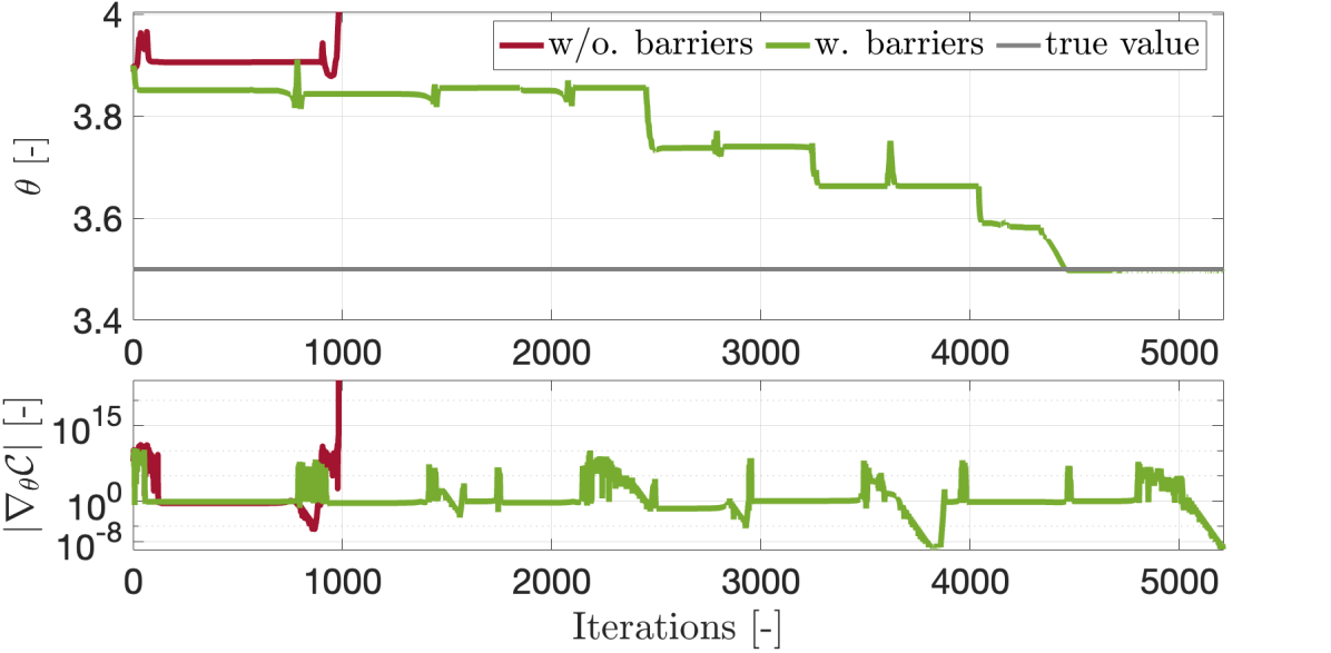
Fig. 2 shows the evolution of the estimated parameters along with the computed gradient when no barrier functions are used (orange line), and when the barrier function proposed in (15) with $\alpha=75$ is adopted in the loss function (green line). It is possible to notice that when no barrier functions are used, the gradient explodes when the estimated parameter reaches the finite-time instability zone with $\theta>4$. On the other hand, the use of an exponential barrier function helps the gradient to steer the parameter in the chaotic area, avoiding values that cause instability, until reaching a neighborhood of the true values.

VI Conclusions

In this paper, we introduced a novel method for solving nonlinear multi-step identification problems by computing exact gradients and leveraging first-order optimization techniques. By modeling the gradient evolution via a linear, time-varying dynamical system, we achieve exact gradient calculation by efficiently exploiting automatic differentiation. The proposed approach allows a detailed analysis of gradient behavior throughout the optimization process, establishing conditions to avoid the exploding gradient phenomenon. Future works will focus on further refining the method and exploring its applicability to a wider range of systems, such as distributed and interconnected systems.

-A Proof of Proposition 1

Consider (4) with $\lambda=\nu=\gamma=0$. The gradient with respect to $\theta$ can be computed as $\nabla_{{\theta}}\mathcal{C}_{T}\doteq\frac{\mathrm{d}\mathcal{C}_{T}}{\mathrm{d}{\theta}}=\frac{\mathrm{d}}{\mathrm{d}{\theta}}\left(\sum_{k=1}^{T}\mathcal{L}_{k}\right)=\sum_{k=0}^{T}\frac{\mathrm{d}\mathcal{L}_{k}}{\mathrm{d}{\theta}}.$ It follows that

$$\nabla_{{\theta}}\mathcal{C}_{k}=\nabla_{{\theta}}\mathcal{C}_{k-1}+\frac{\mathrm{d}\mathcal{L}_{k}}{\mathrm{d}{\theta}},$$ (16)

where $\nabla_{{\theta}}\mathcal{C}_{k}\doteq\sum_{\tau=0}^{k}\frac{\mathrm{d}\mathcal{L}_{\tau}}{\mathrm{d}{\theta}}$ and $\nabla_{{\theta}}\mathcal{C}_{0}=\mathbf{0}_{n_{\theta}}$. Moreover, exploiting the chain rule of differentiation we have the following relation

$$\frac{\mathrm{d}\mathcal{L}_{k}}{\mathrm{d}{\theta}}^{\top} ={\frac{\partial\mathcal{L}_{k}}{\partial{\theta}}}^{\top}+\frac{\partial\mathcal{L}_{k}}{\partial e_{k}}^{\top}\frac{\partial e_{k}}{\partial z_{k}}\frac{\partial z_{k}}{\partial{x_{k}}}\frac{\mathrm{d}{x_{k}}}{\mathrm{d}{\theta}}$$ (17)

where the last term is defined as

$$\frac{\mathrm{d}{x_{k}}}{\mathrm{d}{\theta}}=\frac{\partial{x_{k}}}{\partial{\theta}}+\frac{\partial{x_{k}}}{\partial{x_{k-1}}}\frac{\mathrm{d}x_{k-1}}{\mathrm{d}{\theta}}.$$ (18)

Introducing the recursive memory operator $\Lambda_{k}$ defined in (7), we can rewrite (18) as follows

$$\Lambda_{k}=\frac{\partial{x_{k}}}{\partial{\theta}}+\frac{\partial{x_{k}}}{\partial{x_{k-1}}}\Lambda_{k-1}=\mathcal{J}^{x\!/\!\theta}_{k}+\mathcal{J}^{x\!/\!x}_{k}\Lambda_{k-1},$$

which yields (9a). Thus, (17) can be rewritten as

$$\frac{\mathrm{d}\mathcal{L}_{k}}{\mathrm{d}{\theta}}^{\top}={\nabla_{\theta}^{\top}\mathcal{L}_{k}}+{\nabla_{e}^{\top}\mathcal{L}_{k}}{\mathcal{J}^{e\!/\!z}_{k}}{\mathcal{J}^{z\!/\!x}_{k}}\Lambda^{\top}_{k}=\varrho^{\top}_{k}+\rho^{\top}_{k}\Lambda_{k},$$ (19)

using (8). Thus, (9b) is obtained by transposing and substituting (19) in (16), concluding the proof. $\blacksquare$

-B Proof of Proposition 2

Following the same reasoning of Appendix -A, consider

$$\nabla_{{x_{0}}}\mathcal{C}_{k}=\nabla_{{x_{0}}}\mathcal{C}_{k-1}+\frac{\mathrm{d}\mathcal{L}_{k}}{\mathrm{d}x_{0}}.$$ (20)

Exploiting the chain rule we have

$$\frac{\mathrm{d}\mathcal{L}_{k}}{\mathrm{d}{x}_{0}}^{\top}=\frac{\partial\mathcal{L}_{k}}{\partial e_{k}}^{\top}\frac{\partial e_{k}}{\partial z_{k}}\frac{\partial z_{k}}{\partial{x_{k}}}\frac{\mathrm{d}x_{k}}{\mathrm{d}{x}_{0}},$$ (21)

where the last term is defined as $\frac{\mathrm{d}x_{k}}{\mathrm{d}{x}_{0}}=\frac{\partial x_{k}}{\partial{x_{k-1}}}\frac{\mathrm{d}x_{k-1}}{\mathrm{d}{x}_{0}}.$ Thus, recalling (10), we can write

$$\Lambda_{0,k}=\frac{\partial x_{k}}{\partial{x_{k-1}}}\Lambda_{0,k-1}=\mathcal{J}^{x\!/\!x}_{k}\Lambda_{0,k-1},$$

which yields (11a). Then, (21) can be rewritten as

$$\frac{\mathrm{d}\mathcal{L}_{k}}{\mathrm{d}x_{0}}^{\top}={\nabla_{e}^{\top}\mathcal{L}_{k}}{\mathcal{J}^{e\!/\!z}_{k}}{\mathcal{J}^{z\!/\!x}_{k}}\Lambda_{0,k}=\rho^{\top}_{k}{\Lambda_{0,k}},$$ (22)

using (8). Thus, (11b) is obtained by transposing and substituting (22) in (20). $\blacksquare$

-C Proof of Theorem 1

-C1 Preliminary notions

Given two matrices, $A\in\mathbb{R}^{m,n}$ and $B\in\mathbb{R}^{n,p}$, it is well known that the required computational complexity to perform the multiplication $AB$ is $\mathcal{O}(mnp)$, while the required computational complexity to perform the sum $A+A$ is $\mathcal{O}(mn)$. Similarly, given $C\in\mathbb{R}^{p,q}$, the required computational complexities required to perform $(AB)C$ and $A(BC)$ are $\mathcal{O}(mnp+mpq)=\mathcal{O}(mp(n+q))$ and $\mathcal{O}(npq+mnq)=\mathcal{O}(nq(p+m))$, respectively [19].

-C2 Complexity of (9)

One iteration of (9) involves, in order, the multiplication $m_{1}=\mathcal{J}^{x\!/\!x}_{k}\Lambda_{k-1}$, the sum $\Lambda_{k}=m_{1}+\mathcal{J}^{x\!/\!\theta}_{k}$, the multiplication $m_{2}=\Lambda^{\top}_{k}\rho_{k}$, and the sum $\nabla_{{\theta}}\mathcal{C}_{k}=\nabla_{{\theta}}\mathcal{C}_{k-1}+m_{2}+\varrho_{k}$ with complexities $\mathcal{O}(n_{x}^{2}n_{\theta})$, $\mathcal{O}(n_{x}n_{\theta})$ $\mathcal{O}(n_{x}n_{\theta})$, $\mathcal{O}(2n_{\theta})$, respectively. Thus, the overall complexity for one iteration of (9) is $\mathcal{O}(n_{x}^{2}n_{\theta}+2n_{x}n_{\theta}+2n_{\theta})=\mathcal{O}(n_{x}^{2}n_{\theta})$. It follows that, for $T$ iterations, the required complexity is $\mathcal{O}(Tn_{x}^{2}n_{\theta})$. $\blacksquare$

-D Proof of Theorem 2

We observe that (9b) can be seen as a linear, time-varying (LTV) state-space system with with states $\nabla_{{\theta}}\mathcal{C}_{k}\in\mathbb{R}^{n_{\theta}}$, and

$$A_{k} =A\doteq I_{n_{\theta}}\in\mathbb{R}^{n_{\theta},n_{\theta}},\,B_{k}\doteq(\Lambda^{\top}_{k}\rho_{k}+\varrho_{k})\in\mathbb{R}^{n_{\theta}},$$ (23)

$$C_{k} =C\doteq I_{n_{\theta}}\in\mathbb{R}^{n_{\theta},n_{\theta}},\,D_{k}=D\doteq\mathbf{0}_{n_{\theta}}\in\mathbb{R}^{n_{\theta}},$$

with constant input $u_{k}=1\in\mathbb{R},\forall k\in[0,T]$. By analyzing the BIBO stability properties of the LTV system defined by (23), we can study the exploding gradient phenomenon and obtain conditions under which the multi-step gradient remains bounded. The input-output behavior of (9b) is specified by the unit-pulse response $G(k,j)=C_{k}\Phi(k,j+1)B_{j},$ $k\geq j+1$ with $\Phi(k,j)$ the transition matrix [16]. Stability results are characterized in terms of boundedness properties of $G(k,j)$. From [16, Theorem 27.2] we have that the linear state equation (9b) is uniformly BIBO stable if and only if there exists a finite constant $p$ such that the unit-pulse response satisfies $\sum_{i=j}^{k-1}\|G(k,i)\|\leq p$ for all $k,j$ with $k\geq j+1$. Notice that for our system defined by (23), we have $\Phi(k,j)=I_{n_{\theta}}$, $\forall k,j$, $G(k,j)=B_{j}$, $k\geq j+1,$ that yields (13), concluding the proof. $\blacksquare$

-E Proof of Corollary 1

Considering (13) on the finite time interval $k\in[1,T]$, it is worth noting that the condition holds if $\Lambda_{i}$, $\rho_{i}$, $\varrho_{i}$ are bounded for all $i\in[j,k-1]$, for all possible $k\in[1,T]$ with $k\geq j+1$. The problem is hence reduced to understanding under which conditions $\Lambda_{i}$, $\rho_{i}$, $\varrho_{i}$ may not be bounded. Here, it follows from Lipschitz continuity that the functions $\rho_{k}$, $\varrho_{k}$ (8) are always bounded since $\mathcal{L}_{k}(\cdot)$, $e_{k}$, $h(\cdot)$ are continuously differentiable. On the other hand, the evolution over time of $\Lambda_{k}$ is given by (9a). Here, (9a) can be seen as a linear, time-varying state-space system with states $x_{k}=\text{vec}{(\Lambda_{k})}\in\mathbb{R}^{n_{x}n_{\theta}}$, input $u_{k}=\text{vec}{(\mathcal{J}^{x\!/\!\theta}_{k})}\in\mathbb{R}^{n_{x}n_{\theta}}$, $A_{k}=I_{n_{\theta}}\otimes\mathcal{J}_{k}^{x\!/\!x}\in\mathbb{R}^{n_{x}n_{\theta},n_{x}n_{\theta}}$, where $\text{vec}(\cdot)$ denotes the vectorization of a matrix, i.e., the column vector obtained by stacking the columns of the matrix on top of one another. Here, notice that the stability of this system is directly related to the matrix $\mathcal{J}_{k}^{x\!/\!x}$, corresponding to the linearization of the nonlinear system under analysis around the predicted trajectory obtained with the current values of $\widehat{\theta}$ and $\widehat{x}_{0}$. This links the condition (13) directly to the stability of the predicted trajectories of the system. It follows that for the gradient to be bounded the predicted trajectory must not diverge to infinity within the selected finite multi-step horizon interval, concluding the proof. $\blacksquare$

References

- [1] M. Ahookhosh, “Accelerated first-order methods for large-scale convex optimization: Nearly optimal complexity under strong convexity,” Mathematical Methods of Operations Research, vol. 89, no. 3, pp. 319–353, 2019.
- [2] M. Teboulle, “A simplified view of first order methods for optimization,” Mathematical Programming, vol. 170, no. 1, pp. 67–96, 2018.
- [3] Y. Nesterov, Lectures on convex optimization. Springer, 2018, vol. 137.
- [4] H. Min, R. Vidal, and E. Mallada, “On the convergence of gradient flow on multi-layer linear models,” in International Conference on Machine Learning. PMLR, 2023, pp. 24 850–24 887.
- [5] C. Donati, M. Mammarella, F. Dabbene, C. Novara, and C. Lagoa, “One-shot backpropagation for multi-step prediction in physics-based system identification,” 20th IFAC Symposium on System Identification (SYSID), 2024.
- [6] L. Di Natale, M. Zakwan, B. Svetozarevic, P. Heer, G. Ferrari-Trecate, and C. N. Jones, “Stable linear subspace identification: A machine learning approach,” in 2024 European Control Conference (ECC). IEEE, 2024, pp. 3539–3544.
- [7] T. P. Lillicrap and A. Santoro, “Backpropagation through time and the brain,” Current Opinion in Neurobiology, vol. 55, pp. 82–89, 2019.
- [8] A. G. Baydin, B. A. Pearlmutter, A. A. Radul, and J. M. Siskind, “Automatic differentiation in machine learning: A survey,” Journal of Machine Learning Research, vol. 18, no. 153, pp. 1–43, 2018.
- [9] C. C. Margossian, “A review of automatic differentiation and its efficient implementation,” Wiley interdisciplinary reviews: data mining and knowledge discovery, vol. 9, no. 4, p. 1305, 2019.
- [10] R. Al Seyab and Y. Cao, “Nonlinear system identification for predictive control using continuous time recurrent neural networks and automatic differentiation,” Journal of Process Control, vol. 18, no. 6, pp. 568–581, 2008.
- [11] K. Kaheman, S. L. Brunton, and J. N. Kutz, “Automatic differentiation to simultaneously identify nonlinear dynamics and extract noise probability distributions from data,” Machine Learning: Science and Technology, vol. 3, no. 1, p. 015031, 2022.
- [12] C. Donati, M. Mammarella, F. Dabbene, C. Novara, and C. Lagoa, “Combining off-white and sparse black models in multi-step physics-based systems identification,” Submitted to Automatica, see arXiv:2405.18186, 2024.
- [13] M. Mammarella, C. Donati, F. Dabbene, C. Novara, and C. Lagoa, “A blended physics-based and black-box identification approach for spacecraft inertia estimation,” Accepted for 2024 IEEE Conf. on Decision and Control (CDC), 2024.
- [14] F. Bonassi, M. Farina, J. Xie, and R. Scattolini, “On recurrent neural networks for learning-based control: Recent results and ideas for future developments,” Journal of Process Control, vol. 114, pp. 92–104, 2022.
- [15] L. Behera, S. Kumar, and A. Patnaik, “On adaptive learning rate that guarantees convergence in feedforward networks,” IEEE Trans. on Neural Networks, vol. 17, pp. 1116–1125, 2006.
- [16] W. J. Rugh, Linear system theory. Prentice-Hall, Inc., 1996.
- [17] G.-C. Wu and D. Baleanu, “Discrete fractional logistic map and its chaos,” Nonlinear Dynamics, vol. 75, pp. 283–287, 2014.
- [18] S. C. Phatak and S. S. Rao, “Logistic map: A possible random-number generator,” Physical review E, vol. 51, no. 4, p. 3670, 1995.
- [19] G. H. Golub and C. F. Van Loan, Matrix computations. JHU press, 2013.