Moments of Axial-Vector GPD from Lattice QCD:
Quark Helicity, Orbital Angular Momentum, and Spin-Orbit Correlation

Abstract

In this work, we present a lattice QCD calculation of the Mellin moments of the twist-2 axial-vector generalized parton distribution (GPD), $\widetilde{H}(x,\xi,t)$, at zero skewness, $\xi$, with multiple values of the momentum transfer, $t$. Our analysis employs the short-distance factorization framework on ratio-scheme renormalized quasi-GPD matrix elements. The calculations are based on an $N_{f}=2+1+1$ twisted mass fermions ensemble with clover improvement, a lattice spacing of $a=0.093$ fm, and a pion mass of $m_{\pi}=260$ MeV. We consider both the iso-vector and iso-scalar cases, utilizing next-to-leading-order perturbative matching while ignoring the disconnected contributions and gluon mixing in the iso-scalar case. For the first time, we determine the Mellin moments of $\widetilde{H}$ up to the fifth order. From these moments, we discuss the quark helicity and orbital angular momentum contributions to the nucleon spin, as well as the spin-orbit correlations of the quarks. Additionally, we perform a Fourier transform over the momentum transfer, which allows us to explore the spin structure in the impact-parameter space.

I Introduction

Understanding the internal structure of hadrons, such as protons and neutrons, is a fundamental goal in modern particle and nuclear physics. Generalized parton distributions (GPDs) Müller et al. (1994a); Ji (1997a); Radyushkin (1996a) have emerged as a powerful tool for probing the three-dimensional structure of hadrons. Unlike traditional parton distribution functions (PDFs), which provide information about the longitudinal momentum distribution of partons, GPDs offer a more comprehensive picture by incorporating both longitudinal momentum and transverse spatial distributions Burkardt (2000); Ralston and Pire (2002); Diehl (2002); Burkardt (2003). Therefore, GPDs bridge the gap between the spatial and momentum distributions of quarks and gluons within the nucleon.

The GPDs can be classified into different types based on their symmetry properties twist, and the polarization state of the parton/hadron Diehl (2003); Ji (2004); Belitsky and Radyushkin (2005); Boffi and Pasquini (2007); Mueller (2014); Kumericki et al. (2016). Among these, the twist-2 axial vector GPD $\widetilde{H}(x,\xi,t)$ is crucial for the understanding of the nucleon spin structure, a major challenge in hadronic physics Ashman et al. (1988, 1989). The first Mellin moment of this GPD is directly related to the quark helicity contribution to the nucleon spin, while higher moments provide information on the orbital angular momentum (OAM) Ji (1997a) and spin-orbit correlations of quarks Lorcé (2014); Rajan et al. (2018); Rodekamp et al. (2024), offering essential insights into the spin structure of the nucleon.

In principle, information on the GPDs can be obtained from experimental data for hard exclusive scattering processes such as the deeply virtual Compton scattering Müller et al. (1994b); Ji (1997a); Radyushkin (1996a); Ji (1997b); Collins and Freund (1999), deeply virtual meson production Radyushkin (1996b); Collins et al. (1997); Mankiewicz et al. (1998) and processes where additional particles are detected in the final state Pedrak et al. (2017); Duplančić et al. (2018); Qiu and Yu (2022, 2023a); Duplančić et al. (2023); Qiu and Yu (2023b). However, extracting GPDs from such data is highly non-trivial as it requires solving an inverse problem and disentangling multi-dimensional distributions from limited experimental observables Bertone et al. (2021); Moffat et al. (2023). While much progress has been made in recent years Čuić et al. (2020); Kriesten et al. (2022); Hashamipour et al. (2022); Guo et al. (2022, 2023); Hashamipour et al. (2023); Irani et al. (2023); Čuić et al. (2023), the field is still in its infancy. Consequently, computing GPDs from first principles using lattice QCD is well motivated, as it provides essential complementary information for constraining the GPDs.

Unfortunately, the direct simulation of GPDs is forbidden on a Euclidean lattice as they are defined through non-local light-cone correlators. Therefore, for a long time the focus has been on the Mellin moments of GPDs which can be computed through the matrix elements of local operators Hagler et al. (2003); Brommel et al. (2007); Alexandrou et al. (2011a, 2013); Constantinou (2015); Green et al. (2014); Alexandrou et al. (2017a, b); Hasan et al. (2018); Gupta et al. (2017); Capitani et al. (2019); Alexandrou et al. (2019); Shintani et al. (2019); Bali et al. (2019a, b); Alexandrou et al. (2020a); Jang et al. (2020); Constantinou et al. (2021); Alexandrou et al. (2023); Jang et al. (2024). However, this method encounters difficulties in accessing higher moments due to signal decay and operator mixing under renormalization, which may be mitigated through the application of gradient flow Shindler (2023); Monahan and Orginos (2017) or smearing Davoudi and Savage (2012). Over the past few years, significant progress has been made in computing parton distributions using alternative methods Liu and Dong (1994); Aglietti et al. (1998); Detmold and Lin (2006); Braun and Müller (2008); Ji (2013, 2014); Chambers et al. (2017); Radyushkin (2017); Orginos et al. (2017); Ma and Qiu (2018); Detmold et al. (2021); Gao et al. (2024), especially those motivated by the proposal of quasi-PDFs Ji (2013, 2014). Starting from boosted non-local equal-time correlators, the $x$-dependent parton distributions and their moments can be extracted using the framework of large momentum effective theory (LaMET) Ji et al. (2021) or short distance factorization (SDF) Braun and Müller (2008); Radyushkin (2017); Orginos et al. (2017); Ma and Qiu (2018). For reviews, see Refs. Cichy and Constantinou (2019); Ji et al. (2021); Constantinou (2021); Cichy (2022a, b); Gao (2024).

There has been a lot of progress in computing GPDs through LaMET and SDF in the past few years Chen et al. (2020); Alexandrou et al. (2020b); Lin (2021); Alexandrou et al. (2022); Hannaford-Gunn et al. (2022); Bhattacharya et al. (2021); Lin (2022); Bhattacharya et al. (2022); Constantinou et al. (2023); Bhattacharya et al. (2023a); Cichy et al. (2023); Bhattacharya et al. (2023b, c, 2024a); Dutrieux et al. (2024a); Ding et al. (2024a, b). However, establishing these three-dimensional distributions with comprehensive $x$, $\xi$, and $t$ dependence remains challenging due to the computational cost. Significant progress was made recently in reducing these costs, as originally proposed in Ref. Bhattacharya et al. (2022). By employing the Lorentz-covariant parametrization of matrix elements, quasi-GPDs can be constructed from Lorentz-invariant amplitudes determined from any reference frame. In particular, this innovative approach allows calculations in an asymmetric frame, applying all momentum transfer to the initial-state or final-state nucleon, rather than the commonly used symmetric frame. Consequently, multiple momentum transfers can be achieved through contractions without the need for additional inversions, leading to a faster and more efficient computation of GPDs using lattice QCD. In Refs. Cichy et al. (2023); Bhattacharya et al. (2023b), we presented the $x$-dependent twist-2 unpolarized GPDs $H$ and $E$ with multiple values of momentum transfer $t$ and their moments up to the fifth order. In Ref. Bhattacharya et al. (2024b), we extend the theoretical framework to the case of axial-vector GPDs. Building on this progress, in the present work, we extract the Mellin moments of the zero-skewness axial-vector GPD $\widetilde{H}(x,0,t)$ over a wide range of $t$, and we discuss the physical insights that these moments provide.

This work is organized as follows. In Sec. II, we review the theoretical framework of computing the quasi axial-vector GPD on the lattice. In Sec. III, we show the bare matrix elements of the axial-vector iso-vector and iso-scalar GPDs and discuss the renormalization. In Sec. IV, we extract the first few moments from the ratio-scheme renormalized matrix elements using the next-to-leading order (NLO) SDF formula. For the first time, we get access up to the fifth moment of the axial-vector GPD $\widetilde{H}(x,\xi,t)$ with reasonable signal and $t$ dependence. In Sec. V, we discuss the relation between the moments and the spin structure of the nucleon, including the quark helicity and OAM contributions to the nucleon spin as well as the quark spin-orbit correlations. We also explore the distribution of these quantities in the impact parameter plane. Finally, Sec. VI contains our conclusions.

II Axial-vector GPD on the lattice

II.1 The definition of axial-vector GPDs

The quark GPDs of nucleon are defined as the Fourier transform of the off-forward matrix elements

$$F^{[\Gamma]}(z^{-},\Delta,P)=\langle p_{f};\lambda^{\prime}|O_{\Gamma}|p_{i};\lambda\rangle,$$ (1)

where $p_{i}$ and $p_{f}$ represent the momenta of the initial-state and final-state nucleon, respectively, while $\lambda$ and $\lambda^{\prime}$ denote the helicities of the nucleons. After performing the Fourier transform over $z^{-}$, the GPDs become functions of the average longitudinal momentum fraction $x$ of the quarks and two additional kinematic variables, typically chosen as the skewness $\xi$ and the momentum transfer squared $t$. Using $P=(p_{i}+p_{f})/2$ and $\Delta=p_{f}-p_{i}$, they are defined as

$$\xi=-\frac{\Delta^{+}}{2P^{+}},\quad t=\Delta^{2}.$$ (2)

The quark bilinear operator involved is defined as,

$$O_{\Gamma}=\bar{\psi}(-\tfrac{z^{-}}{2})\Gamma{\cal W}(-\tfrac{z^{-}}{2},\tfrac{z^{-}}{2})\psi(\tfrac{z^{-}}{2}),$$ (3)

where the quark fields are separated along the light-cone and connected by a Wilson line to ensure gauge invariance,

$${\cal W}(-\tfrac{z^{-}}{2},\tfrac{z^{-}}{2})={\cal P}\,{\rm exp}\bigg{(}-ig\int^{\tfrac{z^{-}}{2}}_{-\tfrac{z^{-}}{2}}\,dy^{-}A^{+}(0^{+},y^{-},\vec{0}_{\perp})\bigg{)}\,.$$ (4)

In the light-cone gauge $A^{+}=0$, the Wilson line vanishes, allowing the operator $O_{\Gamma}$ to be interpreted as a particle density operator. For example, setting $\Gamma=\gamma^{+}(1+\gamma_{5})/2$ and $\gamma^{+}(1-\gamma_{5})/2$ corresponds to the density of right-handed and left-handed quarks inside the hadron, respectively. When summed, they give $\Gamma=\gamma^{+}$, providing the total quark number density. Their difference ($\Gamma=\gamma^{+}\gamma_{5}$) yields the quark helicity density, a crucial quantity for understanding the spin structure of the hadron.

In this work, we study the axial-vector GPDs defined through $\Gamma=\gamma^{+}\gamma_{5}$. At the twist-2 level, there are two distinct axial-vector GPDs, $\widetilde{H}$ and $\widetilde{E}$, defined through Diehl (2003)

$$F^{[\gamma^{+}\gamma_{5}]}(z^{-},\Delta,P) =\bar{u}(p_{f},\lambda^{\prime})\bigg{[}\gamma^{+}\gamma_{5}\widetilde{H}(z^{-},\xi,t)+\frac{\Delta^{+}\gamma_{5}}{2m}\widetilde{E}(z^{-},\xi,t)\bigg{]}u(p_{i},\lambda)\,.$$ (5)

Since we are focusing on $\xi=0$ case, the kinematic factor associated with $\widetilde{E}$ vanishes, implying that this GPD cannot be extracted from our lattice data. Here, we therefore concentrate on the GPD $\widetilde{H}$. We note that $\widetilde{E}$ also enters at the twist-3 level, where it can be addressed even for $\xi=0$ Kiptily and Polyakov (2004); Bhattacharya et al. (2023c).

II.2 The axial-vector quasi GPD $\widetilde{\cal H}$

The light-cone GPDs can be accessed from lattice QCD through the quasi-GPD approach in the large momentum limit. However, unlike light-cone GPDs, which are frame-independent, quasi-GPDs are frame-dependent at finite momentum. Traditionally, a specific symmetric frame was chosen. However, this choice is computationally very expensive, requiring separate, full computations—including inversions and contractions on the lattice—for each value of $t$. To address this problem, we proposed constructing quasi-GPDs using Lorentz-invariant amplitudes derived from the decomposition of the matrix elements Bhattacharya et al. (2022). This method eliminates the frame dependence, allowing any computationally preferred frame to be used. It is important to note that this decomposition is not unique and depends on the choice of basis. However, any basis will result in the same number of independent amplitudes. For the axial current we adopted the following decomposition Bhattacharya et al. (2024b),

$${F}^{[\gamma^{\mu}\gamma_{5}]}(z,P,\Delta) \equiv\langle p_{f};\lambda^{\prime}|\bar{\psi}(-\tfrac{z}{2})\,\gamma^{\mu}\gamma_{5}\,{\cal W}(-\tfrac{z}{2},\tfrac{z}{2})\psi(\tfrac{z}{2})|p_{i};\lambda\rangle$$

$$=\bar{u}(p_{f},\lambda^{\prime})\bigg{[}\dfrac{i\epsilon^{\mu Pz\Delta}}{m}\widetilde{A}_{1}+\gamma^{\mu}\gamma_{5}\widetilde{A}_{2}+\gamma_{5}\bigg{(}\dfrac{P^{\mu}}{m}\widetilde{A}_{3}+mz^{\mu}\widetilde{A}_{4}+\dfrac{\Delta^{\mu}}{m}\widetilde{A}_{5}\bigg{)}$$

$$\hskip 46.94687pt+m\not{z}\gamma_{5}\bigg{(}\dfrac{P^{\mu}}{m}\widetilde{A}_{6}+mz^{\mu}\widetilde{A}_{7}+\dfrac{\Delta^{\mu}}{m}\widetilde{A}_{8}\bigg{)}\bigg{]}u(p_{i},\lambda),$$ (6)

where $\epsilon^{\mu Pz\Delta}=\epsilon^{\mu\alpha\beta\gamma}P_{\alpha}z_{\beta}\Delta_{\gamma}$ and $\widetilde{A}_{i}\equiv\widetilde{A}_{i}(z\cdot P,z\cdot\Delta,\Delta^{2},z^{2})$ are Lorentz invariant amplitudes that depend on Lorentz scalars. The case of the light-cone axial-vector GPDs defined in Eq. (5) corresponds to $\mu=+$ and $z=(z^{+},z^{-},z_{\perp})=(0,z^{-},0_{\perp})$. Thus, the GPD $\widetilde{H}$ can be expressed as

$$\widetilde{H}(z\cdot P,z\cdot\Delta,\Delta^{2}) =\widetilde{A}_{2}+(P^{+}z^{-})\widetilde{A}_{6}+(\Delta^{+}z^{-})\widetilde{A}_{8}$$

$$=\widetilde{A}_{2}+(P\cdot z)\widetilde{A}_{6}+(\Delta\cdot z)\widetilde{A}_{8}.$$ (7)

As mentioned earlier, light-cone GPDs cannot be directly simulated in Euclidean lattice QCD. In this work, we consider quasi-GPDs, which maintain the same form as Eq. (5) but are defined at equal time ($z^{0}=0$). In this approach, quarks are separated along the spatial direction $\mathbf{z}=(0,0,z^{3})$ with a large momentum $\mathbf{P}=(0,0,P^{3})$. Typically, $\gamma^{\mu}\gamma_{5}=\gamma^{3}\gamma_{5}$ is chosen to approach the light-cone limit, as it avoids operator mixing caused by explicit chiral symmetry breaking which affects $\gamma^{0}\gamma_{5}$ Constantinou and Panagopoulos (2017); Chen et al. (2018). This means, we consider

$$F^{[\gamma^{3}\gamma_{5}]}(z,P,\Delta) =\bar{u}(p_{f},\lambda^{\prime})\bigg{[}\gamma^{3}\gamma_{5}\widetilde{\cal H}_{3}(z,\xi,t)+\frac{\Delta^{3}\gamma_{5}}{2m}\widetilde{\cal E}_{3}(z,\xi,t)\bigg{]}u(p_{i},\lambda)\,.$$ (8)

According to Eq. (6), the axial-vector quasi GPDs can be expressed as

$$\widetilde{\mathcal{H}}_{3}(z,P,\Delta) =\widetilde{A}_{2}-z^{3}P^{3}\widetilde{A}_{6}-m^{2}(z^{3})^{2}\widetilde{A}_{7}-z^{3}\Delta^{3}\widetilde{A}_{8}$$

$$=\widetilde{A}_{2}+(P\cdot z)\widetilde{A}_{6}+m^{2}z^{2}\widetilde{A}_{7}+(\Delta\cdot z)\widetilde{A}_{8}.$$ (9)

Compared to Eq. (7), the Lorentz invariant amplitudes $\widetilde{A}_{i}(z\cdot P,z\cdot\Delta,\Delta^{2},z^{2})$ in $\widetilde{\mathcal{H}}_{3}$ implicitly depend on the finite $z^{2}=-|\mathbf{z}|^{2}$, which is zero in the light-cone case. In addition, $\widetilde{\mathcal{H}}_{3}$ explicitly includes an additional contamination term $m^{2}z^{2}\widetilde{A}_{7}$ due to the non-vanishing $z^{2}$. In Refs. Bhattacharya et al. (2022, 2024b), it was proposed to remove these explicit power corrections and construct Lorentz-invariant (LI) matrix elements, as in Eq. (7), through the Lorentz-invariant amplitudes $\widetilde{A}_{i}$, which can be extracted from the linear combination of quasi-GPDs with different spin structures. As discussed in detail in Ref. Bhattacharya et al. (2024b), the LI axial-vector GPDs in Eq. (7) can be derived from the linear combination of $F^{[\gamma^{\mu}\gamma_{5}]}$ with $\mu=0,1,2$, referred to as $\widetilde{\mathcal{H}}$. We note that the only difference between the quasi GPD $\widetilde{\mathcal{H}}$ and light-cone GPD $\widetilde{{H}}$ is the non-zero $z^{2}$ in $\widetilde{A}_{i}$. Interestingly, it was found in Ref. Bhattacharya et al. (2024b) that the term $m^{2}z^{2}\widetilde{A}_{7}$ is mostly consistent with zero, so that $\widetilde{\mathcal{H}}_{3}$ and $\widetilde{\mathcal{H}}$ are largely consistent within statistical errors. Therefore, we can focus on $\widetilde{\mathcal{H}}_{3}$ in the following analysis without concerns about the contamination term $m^{2}z^{2}\widetilde{A}_{7}$. Additionally, we repeat that $\widetilde{\mathcal{H}}_{3}$ has the advantage of avoiding operator mixing due to explicit chiral symmetry breaking from lattice discretization Constantinou and Panagopoulos (2017); Chen et al. (2018).

III Bare matrix elements and renormalization

III.1 Lattice setup

The data used in this work has been analyzed in Ref. Bhattacharya et al. (2024b), to derive the $x$-dependent GPD in the LaMET framework. In this study, however, we focus on extracting the first few moments of GPDs using the SDF approach. The data was obtained from a gauge ensemble of $N_{f}=2+1+1$ twisted-mass fermions with a clover term and Iwasaki-improved gluons Alexandrou et al. (2018). The lattice size and spacing of the ensemble are $N_{s}\times N_{t}=32^{3}\times 64$ and $a$ = 0.0934 fm, respectively, with quark masses corresponding to a pion mass of 260 MeV.

frame	$P_{3}$ [GeV]	$\quad\mathbf{\Delta}$ $[\frac{2\pi}{L}]\quad$	$-t$ [GeV2]	$\quad\xi\quad$	$N_{\rm ME}$	$N_{\rm confs}$	$N_{\rm src}$	$N_{\rm tot}$
N/A	$\pm$1.25	(0,0,0)	0	0	2	329	16	10528
symm	$\pm$0.83	($\pm$2,0,0), (0,$\pm$2,0)	0.69	0	8	67	8	4288
symm	$\pm$1.25	($\pm$2,0,0), (0,$\pm$2,0)	0.69	0	8	249	8	15936
symm	$\pm$1.67	($\pm$2,0,0), (0,$\pm$2,0)	0.69	0	8	294	32	75264
symm	$\pm$1.25	$(\pm 2,\pm 2,0)$	1.38	0	16	224	8	28672
symm	$\pm$1.25	($\pm$4,0,0), (0,$\pm$4,0)	2.77	0	8	329	32	84224
asymm	$\pm$1.25	($\pm$1,0,0), (0,$\pm$1,0)	0.17	0	8	269	8	17216
asymm	$\pm$1.25	$(\pm 1,\pm 1,0)$	0.34	0	16	195	8	24960
asymm	$\pm$1.25	($\pm$2,0,0), (0,$\pm$2,0)	0.65	0	8	269	8	17216
asymm	$\pm$1.25	($\pm$1,$\pm$2,0), ($\pm$2,$\pm$1,0)	0.81	0	16	195	8	24960
asymm	$\pm$1.25	($\pm$2,$\pm$2,0)	1.24	0	16	195	8	24960
asymm	$\pm$1.25	($\pm$3,0,0), (0,$\pm$3,0)	1.38	0	8	269	8	17216
asymm	$\pm$1.25	($\pm$1,$\pm$3,0), ($\pm$3,$\pm$1,0)	1.52	0	16	195	8	24960
asymm	$\pm$1.25	($\pm$4,0,0), (0,$\pm$4,0)	2.29	0	8	269	8	17216

Table 1: Statistics for the symmetric and asymmetric frame matrix elements are shown. The momentum unit $2\pi/L$ is 0.417 GeV. $N_{\rm ME}$, $N_{\rm confs}$, $N_{\rm src}$ and $N_{\rm total}$ are the number of matrix elements, configurations, source positions per configuration and total statistics, respectively.

The quasi-GPD matrix elements are extracted from the three-point functions,

$$\begin{split}C^{\rm 3pt}_{\mu}(\Gamma_{\kappa},p_{f},p_{i};t_{s},\tau)=\sum_{\vec{y},\vec{z}_{0}}e^{-i\vec{p}_{f}\cdot(\vec{y}-\vec{x})}e^{-i\vec{q}\cdot(\vec{x}-\vec{z}_{0})}\Gamma^{\kappa}_{\alpha\beta}\langle{N_{\alpha}(\vec{y},t_{s})\mathcal{O}_{\mu}(\vec{z}_{0}+z\hat{z},\tau)\overline{N}_{\beta}(\vec{x},0)}\rangle,\end{split}$$ (10)

where $\vec{x}$ is the source position, $N^{(s)}$ is the standard nucleon source under momentum smearing Bali et al. (2016) to improve the overlap with the proton ground state and suppress gauge noise. The quasi-GPD operator $\mathcal{O}_{\mu}=\bar{\psi}\left(z\right)\gamma^{\mu}\gamma_{5}{\cal W}(0,z)\psi\left(0\right)$ has quark fields separated along the $z_{3}$ direction. Both the iso-vector ($u-d$) and iso-scalar ($u+d$) flavor combinations were computed with the disconnected diagrams ignored for the iso-scalar case. In Ref. Alexandrou et al. (2021), it was found that, on the same ensemble as this work, the disconnected contributions for the forward limit are tiny; they would be further suppressed in off-forward kinematics. The unpolarized and polarized parity projectors $\Gamma_{0}$ and $\Gamma_{\kappa}$ are defined as,

$$\Gamma_{0} =\frac{1}{4}\left(1+\gamma_{0}\right)\,,$$ (11)

$$\Gamma_{\kappa} =\frac{1}{4}\left(1+\gamma_{0}\right)i\gamma_{5}\gamma_{\kappa}\,,\quad\kappa=1,2,3\,.$$ (12)

To derive the ground-state matrix elements, we also computed the two-point functions for the energy spectrum and overlap amplitudes $\langle\Omega|N^{(s)}|N\rangle$, which are given by,

$$\begin{split}C^{\rm 2pt}(\Gamma_{0},p;t_{s})=\sum_{\vec{y}}e^{-i\vec{p}\cdot(\vec{y}-\vec{x})}\Gamma^{0}_{\alpha\beta}\langle{N^{(s)}_{\alpha}(\vec{y},t_{s})\overline{N}^{(s^{\prime})}_{\beta}(\vec{x},0)}\rangle\,.\end{split}$$ (13)

Since the two- and three-point functions are highly correlated, we construct the ratio,

$$R^{\mu}_{\kappa}(\Gamma_{\kappa},p_{f},p_{i};t_{s},\tau)=\frac{C^{\rm 3pt}_{\mu}(\Gamma_{\kappa},p_{f},p_{i};t_{s},\tau)}{C^{\rm 2pt}(\Gamma_{0},p_{f};t_{s})}\sqrt{\frac{C^{\rm 2pt}(\Gamma_{0},p_{i},t_{s}-\tau)C^{\rm 2pt}(\Gamma_{0},p_{f},\tau)C^{\rm 2pt}(\Gamma_{0},p_{f},t_{s})}{C^{\rm 2pt}(\Gamma_{0},p_{f},t_{s}-\tau)C^{\rm 2pt}(\Gamma_{0},p_{i},\tau)C^{\rm 2pt}(\Gamma_{0},p_{i},t_{s})}}\,,$$ (14)

which, in the $t_{s}\rightarrow\infty$ limit, corresponds to the bare matrix elements of proton ground state matrix elements $\lim\limits_{t_{s}\rightarrow\infty}R^{\mu}_{\kappa}=\Pi_{\mu}(\Gamma_{\kappa})$. To keep the statistical noise under control, we use a source-sink separation of $t_{s}=10a=0.93$ fm and perform a plateau fit with respect to the time insertion $\tau$ in a region of convergence. More details can be found in Ref. Bhattacharya et al. (2024b). A more thorough study of excited state contamination will be left for future work that targets precision control.

In Table 1, we show the momenta $\vec{P}=(0,0,P_{3})$ and $\vec{\Delta}$ as well as the statistics used in this work. For the symmetric frame, the momentum components are defined as,

$$\vec{p}^{\,s}_{f}=\vec{P}+\frac{\vec{\Delta}}{2}=\left(+\frac{\Delta_{1}}{2},+\frac{\Delta_{2}}{2},P_{3}\right)\,,\qquad\vec{p}^{\,s}_{i}=\vec{P}-\frac{\vec{\Delta}}{2}=\left(-\frac{\Delta_{1}}{2},-\frac{\Delta_{2}}{2},P_{3}\right)\,,$$ (15)

In contrast, for the asymmetric frame, where all momentum transfer is assigned to the initial state, we have,

$$\vec{p}^{\,a}_{f}=\vec{P}=\left(0,0,P_{3}\right)\,,\qquad\vec{p}^{\,a}_{i}=\vec{P}-\vec{\Delta}=\left(-\Delta_{1},-\Delta_{2},P_{3}\right)\,.$$ (16)

While $\vec{P}$ and $\vec{\Delta}$ are the same for both frames, they lead to slightly different values of $-t$ due to the different distribution of the momentum transfer, that is

$$-t^{s}=\vec{\Delta}^{2}\,,\qquad-t^{a}=\vec{\Delta}^{2}-(E(p^{\prime})-E(p))^{2}\,.$$ (17)

This work focuses on zero skewness, namely $\Delta_{3}=0$. As already mentioned above, this does not give us access to the GPD $\widetilde{E}$. Most of the hadron momentum $P$ is fixed at 1.25 GeV throughout the calculation. We combine all data contributing to the same value of momentum transfer $t=-\Delta^{2}$ with definite symmetry with respect to $P_{3}\to-P_{3}$, $z_{3}\to-z_{3}$, and $\vec{\Delta}\to-\vec{\Delta}$ Bhattacharya et al. (2024b).

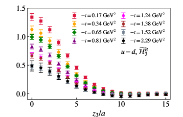
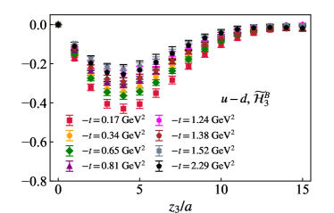
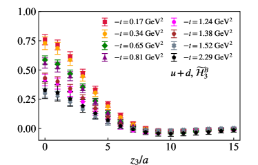
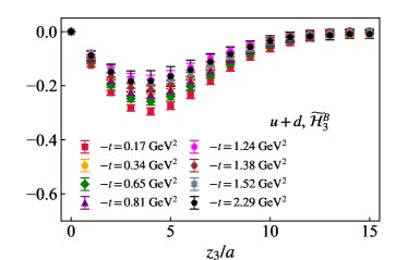
Figure 1: Bare matrix elements are shown as a function of $z_{3}/a$ for different values of $t$. The iso-vector ($u-d$) and iso-scalar ($u+d$) case are shown in the upper and lower panels, respectively. The left panels show the real part while the right panels show the imaginary part.

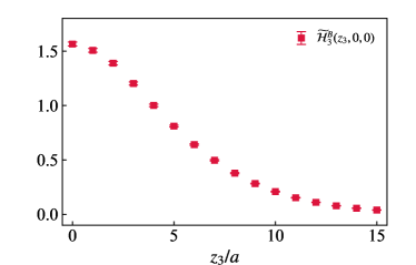
Figure 2: Zero momentum iso-vector axial-vector quasi-PDF matrix elements.

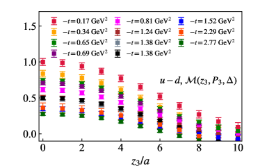
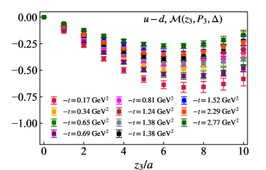
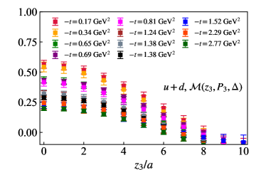
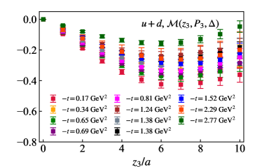
Figure 3: Ratio scheme renormalized matrix elements are shown as a function of $z_{3}/a$. The iso-vector ($u-d$) and iso-scalar ($u+d$) case are shown in the upper and lower panels, respectively. The left panels show the real part while the right panels show the imaginary part.

III.2 Bare matrix elements and renormalization

The bare matrix elements for the quasi axial-vector GPD $\widetilde{\mathcal{H}}_{3}$ are shown in Fig. 1, where a clear signal is observed across a wide range of momentum transfers $-t$. The bare matrix elements need to be renormalized. At $z=0$ and $\Delta=0$, the iso-vector matrix element $\widetilde{\mathcal{H}}_{3}^{B}$ gives the bare iso-vector axial charge of the nucleon, $g_{A}^{B}$, which needs to be renormalized by the constant $Z_{A}$. The $Z_{A}$ for this ensemble has been determined as 0.7442 Bhattacharya et al. (2024b), leading to a derived $g_{A}=1.164(13)$ using $\widetilde{\mathcal{H}}_{3}^{B,u-d}(0,0,0)$. This value is consistent with results in Ref. Alexandrou et al. (2011b) with similar quark masses. For the case of non-zero $z_{3}$, it has been shown that the non-local operator $O_{\Gamma}$ can be multiplicatively renormalized Ji et al. (2018); Green et al. (2018); Ishikawa et al. (2017),

$$O_{\Gamma}(z)=Z_{O}e^{-\delta m|z|}O_{\Gamma}^{R}(z),$$ (18)

where $Z_{O}$ accounts for logarithmic divergences, and the exponential factor $e^{-\delta m|z|}$ removes the linear divergence stemming from the self-energy of the spatial Wilson link. Since this renormalization is independent of the hadron state and quark flavor, one can construct an appropriate ratio to eliminate UV divergences and obtain renormalization group invariant quantities Fan et al. (2020); Radyushkin (2017); Orginos et al. (2017); Gao et al. (2020),

$$\mathcal{M}(z_{3},P_{3},\Delta)=\frac{\widetilde{\mathcal{H}}_{3}^{B}(z_{3},P_{3},\Delta;a)}{\widetilde{\mathcal{H}}_{3}^{B}(z_{3},0,0;a)}\cdot g_{A}=\frac{\widetilde{\mathcal{H}}_{3}^{R}(z_{3},P_{3},\Delta;\mu)}{\widetilde{\mathcal{H}}_{3}^{R}(z_{3},0,0;\mu)}\cdot g_{A}.$$ (19)

We multiply $g_{A}=Z_{A}\widetilde{\mathcal{H}}_{3}^{B,u-d}(0,0,0;a)$ to normalize the iso-vector $\mathcal{M}(0,0,0)$ to $g_{A}$. This choice of convention will be explained in the next section. In this ratio, the matrix elements in the denominator correspond to axial-vector quasi-PDF matrix elements with zero momentum $P=0$ and zero momentum transfer $\Delta=0$. Since UV divergences are independent of the light quark flavors, we consistently use the iso-vector $\widetilde{\mathcal{H}}_{3}^{B,u-d}(z_{3},0,0)$ as the denominator in this work, which are shown in Fig. 2. Both the iso-vector and iso-scalar $\widetilde{\mathcal{H}}_{3}^{B}(z,P,\Delta)$ are used in the numerator. It should be noted again that the disconnected diagrams were omitted for the iso-scalar case in this study.

In Fig. 3, the real and imaginary parts of the ratio scheme renormalized matrix elements are presented as a function of $z_{3}$ for both the iso-vector and iso-scalar cases. As one can see, the expected $-t$ dependence is clearly visible, with the amplitude of the matrix elements decreasing monotonically as $-t$ increases.

IV Mellin moments from short distance factorization

IV.1 Short distance factorization

In the short-distance limit, the renormalized matrix elements can be expanded in terms of the Mellin moments using the operator product expansion (OPE). For the zero-skewness quasi-GPD under consideration, the OPE structure mirrors that of the quasi-PDF case, without any mixing between moments. In the $\overline{\rm MS}$ scheme, the short-distance factorization (SDF) of the iso-vector quasi-GPD matrix elements can be expressed as,

$$\widetilde{\mathcal{H}}_{3}^{R}(z_{3},P_{3},\Delta;\mu)=\sum_{n=0}^{\infty}C_{n}^{\overline{\rm MS}}(\mu^{2}z^{2})\frac{(-iz_{3}P_{3})^{n}}{n!}\tilde{A}_{n+1,0}(t;\mu)+\mathcal{O}(\Lambda_{\rm QCD}^{2}z^{2}),$$ (20)

where the

$$\tilde{A}_{n+1,0}(t;\mu)=\int_{-1}^{1}dxx^{n}\widetilde{H}(x,\xi=0,t;\mu)$$ (21)

represent the Mellin moments of the axial-vector GPD at zero skewness. It’s worth to mention that the first moment $\tilde{A}_{1,0}(t;\mu)$ is the nucleon axial form factor corresponding to the local matrix elements $\widetilde{\mathcal{H}}_{3}^{R}(0,P_{3},\Delta;\mu)$. $C_{n}(\mu^{2}z^{2})$ are the Wilson coefficients. At leading order (LO), $C_{n}(\mu^{2}z^{2})=1$, making Eq. (20) a simple polynomial function of the so-called Ioffe time $\zeta=z_{3}P_{3}$. Beyond LO, the perturbative corrections account for the scale evolution from the physical scale $\sim 1/z_{3}$ to the factorization scale $\mu$, which at NLO are given by Izubuchi et al. (2018),

$$\begin{split}C_{n}^{\overline{\rm MS}}(\mu^{2}z^{2})=1+\frac{\alpha_{s}C_{F}}{2\pi}\bigg{[}\bigg{(}\frac{3+2n}{2+3n+n^{2}}+2H_{n}\bigg{)}L_{z}+\frac{7+2n}{2+3n+n^{2}}+2(1-H_{n})H_{n}-2H^{(2)}_{n}\bigg{]},\end{split}$$ (22)

with $L_{z}=\ln(\mu^{2}z^{2}e^{2\gamma_{E}}/4)$ and the Harmonic numbers $H_{n}=\sum_{i=1}^{n}1/i$ and $H_{n}^{(2)}=\sum_{i=1}^{n}1/i^{2}$. This SDF formula can be inserted into Eq. (19), establishing a relationship between the renormalized matrix elements and the moments of the GPDs,

$$\begin{split}\mathcal{M}(z_{3},P_{3},\Delta)&=\frac{\sum_{n=0}^{\infty}C_{n}^{\overline{\rm MS}}(\mu^{2}z^{2})\frac{(-iz_{3}P_{3})^{n}}{n!}\tilde{A}_{n+1,0}(t;\mu)+\mathcal{O}(\Lambda_{\rm QCD}^{2}z^{2})}{C_{0}^{\overline{\rm MS}}(\mu^{2}z^{2})\tilde{A}_{1,0}^{u-d}(0;\mu)+\mathcal{O}(\Lambda_{\rm QCD}^{2}z^{2})}\cdot g_{A}\\ &=\sum_{n=0}^{\infty}\frac{C_{n}^{\overline{\rm MS}}(\mu^{2}z^{2})}{C_{0}^{\overline{\rm MS}}(\mu^{2}z^{2})}\frac{(-iz_{3}P_{3})^{n}}{n!}\tilde{A}_{n+1,0}(t)+\mathcal{O}(\Lambda_{\rm QCD}^{2}z^{2}).\end{split}$$ (23)

We note again, the denominator in Eq. (19) is solely the iso-vector matrix element while the numerator can be either iso-vector and iso-scalar. As a result, $\tilde{A}_{1,0}^{u-d}(0;\mu)=g_{A}$ cancels out in the first line of the formula. This explain our choice of ratio defined in Eq. (19). From this expression, the even and odd moments of the axial-vector GPD can be extracted from the real and imaginary parts of $\mathcal{M}(z_{3},P_{3},\Delta)$, respectively. Notably, it is crucial to keep $z^{2}$ small to avoid large power corrections. At present, lattice calculations are limited to finite values of $P_{3}$, which in our case are listed in Table 1, allowing the extraction of only the first few moments within a limited kinematic range of $z_{3}P_{3}$.

IV.2 Moments from fixed $z^{2}$

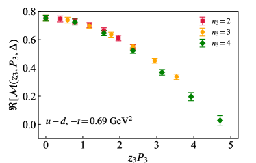
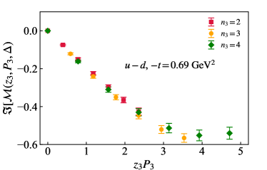
Figure 4: The ratio scheme renormalized iso-vector matrix elements for $-t=0.69~{}\rm GeV^{2}$ are shown as a function of $z_{3}P_{3}$ for three different values of $P_{3}$. The real part (left panel) and imaginary part (right panel) are both shown.

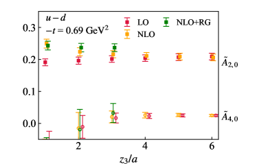
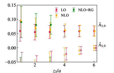
Figure 5: The iso-vector moments at momentum transfer $-t=0.69~{}\rm GeV^{2}$, derived from fits of $P_{3}$ dependence, are shown as a function of $z_{3}$.

For $-t=0.69\rm GeV^{2}$, we have three different momenta with $n_{3}=2,\,3,\,4$ corresponding to 0.83, 1.25, 1.67 GeV, respectively. This allows us to extract moments from each single $z_{3}$ by fitting the $P_{3}$ dependence. In this section, we consider the matching formula at LO, NLO, as well as renormalization group improved NLO (NLO+RG) Gao et al. (2021); Su et al. (2023); Dutrieux et al. (2024b, a) accuracy. If the perturbative matching can describe the evolution well, the moments for a given factorization scale $\mu$ should be independent for different values of $z_{3}$.

In Fig. 4, we present the ratio scheme renormalized matrix elements for the iso-vector case as a function of $z_{3}P_{3}$. One can see from the plots that the dependence of the results on $P_{3}$ is very weak. This is expected, because in absence of evolution encoded in $C_{n}^{\overline{\rm MS}}(\mu^{2}z^{2})$, the renormalized matrix element should be a function of $z_{3}P_{3}$ only. To extract the moments according to Eq. (23), we minimize,

$$\chi^{2}_{z_{3}}=\sum_{P_{3}}\bigg{(}\frac{(\real[\mathcal{M}^{\rm data}(z_{3},P_{3},\Delta)]-\real[\mathcal{M}^{\rm SDF}(z_{3},P_{3},\Delta)])^{2}}{\sigma_{\real}^{2}}+\frac{(\imaginary[\mathcal{M}^{\rm data}(z_{3},P_{3},\Delta)]-\imaginary[\mathcal{M}^{\rm SDF}(z_{3},P_{3},\Delta)])^{2}}{\sigma_{\imaginary}^{2}}\bigg{)},$$ (24)

where $\sigma_{\real}$ and $\sigma_{\imaginary}$ represent the errors in the real and imaginary parts of $\mathcal{M}^{\rm data}(z_{3},P_{3},\Delta)$, respectively.

The moments obtained from the fits are shown in Fig. 5 as a function of $z_{3}$. The results are evaluated at $\mu=2$ GeV. We omit the discussion of the axial form factor $\tilde{A}_{1,0}$ here, as it is determined from local matrix elements, requiring neither the SDF nor dependence on $z_{3}$. For the first two non-trivial moments, $\tilde{A}_{2,0}$ and $\tilde{A}_{3,0}$, a reasonable signal emerges starting from $z_{3}=a$. However, for the higher moments a clear signal can only be obtained for larger values of $z_{3}$. As one can see, $\tilde{A}_{2,0}$ exhibits a mild $z_{3}$ dependence for $z_{3}<4a$ when LO and NLO Wilson coefficients are used. This mild dependence is due to a combination of discretization effects, which could be especially large for $z_{3}=a$, and missing higher-order terms in the Wilson coefficients. The results that use NLO Wilson coefficients with RG improved coefficients are only shown for $z_{3}$ up to $3a$, as for larger $z_{3}$ values the scale is too low to evaluate the strong coupling constant $\alpha_{s}$. In that range, the NLO results and NLO results with RG resummation are consistent.

IV.3 Moments from combined fits

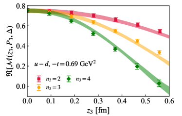
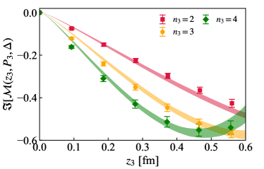
Figure 6: The ratio scheme renormalized iso-vector matrix elements for the case with momentum transfer $-t=0.69\rm GeV^{2}$ are shown as a function of $z_{3}$ for three different values of $P_{3}$. The real part (left panel) and imaginary part (right panel) are both shown. The bands are reconstructed from the fit with $z_{3}\in[2a,6a]$ including the NLO matching kernels.

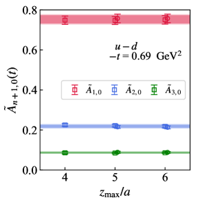
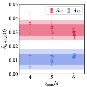
Figure 7: The moments obtained from combineds fit using matrix element with $z_{3}\in[z_{\rm min},z_{\rm max}]$ and $n_{3}=2,3,4$ are shown as a function of $z_{\rm max}$. The squared symbols are results from $z_{\rm min}=2a$ while the circled symbols are from $z_{\rm min}=3a$.

Since the factorization formula with NLO coefficient can describe the lattice data reasonably well, in this section we perform combined fits of matrix elements with different $n_{3}$ in a range of $z_{3}\in[z_{\rm min},z_{\rm max}]$. Specifically, we minimize the $\chi^{2}=\sum_{z_{3}}\chi^{2}_{z_{3}}$. The combined fits are more stable than the fits for fixed $z_{3}$ values. To avoid the most serious discretization effects, we skip the point $z_{3}=a$. We vary $z_{\rm min}\in[2a,3a]$ to estimate the discretization effects and $z_{\rm max}\in[z_{\rm min}+2a,6a]$ to estimate the higher-twist effects. The resulting fit yields a reasonable $\chi^{2}/{\rm d.o.f.}$, and the bands reconstructed from the fit accurately describe the renormalized matrix elements, as shown in Fig. 6.

The extracted moments are shown in Fig. 7. The squared symbols represent results from $z_{\rm min}=2a$, while the circled symbols correspond to $z_{\rm min}=3a$. As illustrated, the results from the two $z_{\rm min}$ values overlap, indicating that discretization effects are minimal compared to the statistical errors. Regarding the $z_{\rm max}$ dependence, it appears negligible within the errors, particularly for the lower moments. However, higher moments require larger $z_{\rm max}$ values to stabilize the fit.

For the final estimates, we average the results obtained from different choices of $z_{\rm min}$ and $z_{\rm max}$, with their deviations treated as systematic errors, as we did in Refs. Gao et al. (2020); Bhattacharya et al. (2023b). These results are depicted as bands in Fig. 7, with the darker and lighter bands representing statistical and systematic errors, respectively, covering the relevant data points.

We extended this analysis to all other values of the momentum transfer listed in Table 1, covering both iso-vector and iso-scalar cases. For the latter, we neglected the mixing with the gluon distribution starting from $\mathcal{O}(\alpha_{s})$ Yao et al. (2023). In Fig. 8, we summarize our determination of first two moments, $\tilde{A}_{1,0}$ and $\tilde{A}_{2,0}$, as functions of $-t$. For comparison, we show results obtained from traditional local operator methods with a similar lattice setup and pion mass for the iso-vector case (ETMC) Alexandrou et al. (2011b); Baran et al. (2011). It is encouraging that our results align with the previous ETMC findings, suggesting that our extraction of the moments from non-local operators is effective. Notably, we are also able to extract higher moments up to $\tilde{A}_{5,0}$ for the first time, as shown in Fig. 9. As one can see from the figure, we obtain a reasonable signal, and the $-t$ dependence of the results follows the general expectations. We note that we apply the $z$-expansion and a dipole fit, and for each we compare the parametrization of the $t$ dependence using data up to 1.0 GeV² and 1.5 GeV². In most cases, the dipole fit and the $z$-expansion are in agreement. However, a difference is found between $-t_{\rm max}=1.0$ GeV² and $-t_{\rm max}=1.5$ GeV². More details are given in Sec.V.1.

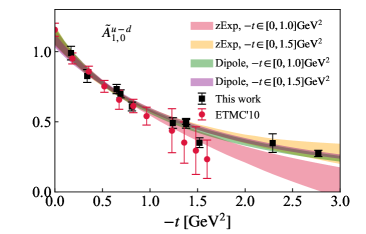
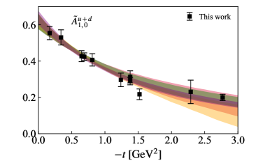
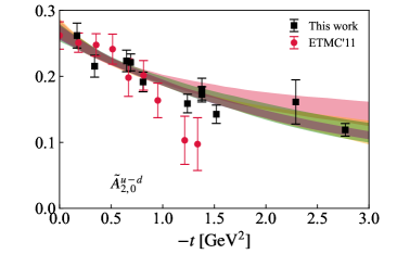
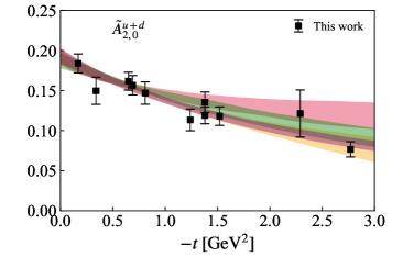
Figure 8: The first and second Mellin moments $\tilde{A}_{1,0}$ and $\tilde{A}_{2,0}$ of the axial-vector GPDs are shown. The left panels are the iso-vector results while the right panels are the iso-scalar results. The bands are results from $z$-expansion (zExp) and dipole methods by fitting data in the ranges $-t\in[0,1.0]~{}\rm{GeV}^{2}$ and $-t\in[0,1.5]~{}\rm{GeV}^{2}$. For comparison, we also show results derived from traditional local operator methods with the same pion mass for the iso-vector case (ETMC) Alexandrou et al. (2011b); Baran et al. (2011).

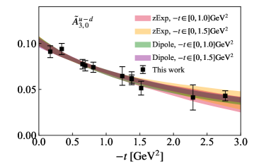
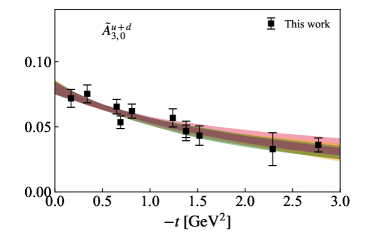
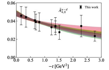
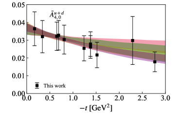
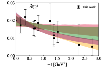
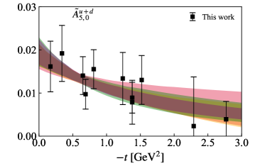
Figure 9: The Mellin moments $\tilde{A}_{3,0}$, $\tilde{A}_{4,0}$ and $\tilde{A}_{5,0}$ of the axial-vector GPDs are shown. The left panels are the iso-vector results while the right panels are the iso-scalar results. The bands are results from $z$-expansion (zExp) and dipole methods by fitting data in the ranges $-t\in[0,1.0]~{}\rm{GeV}^{2}$ and $-t\in[0,1.5]~{}\rm{GeV}^{2}$.

V Insights into nucleon spin dynamics from axial vector GPD

GPDs offer crucial insights into the spin structure of the nucleon. For instance, in a longitudinally polarized nucleon, the contributions to the nucleon spin $\textbf{S}^{N}_{z}$ from quark helicity, orbital angular momentum (OAM), and total spin are represented by $\langle\textbf{S}^{q}_{z}\textbf{S}^{N}_{z}\rangle$, $\langle\textbf{L}^{q}_{z}\textbf{S}^{N}_{z}\rangle$ and $\langle\textbf{J}^{q}_{z}\textbf{S}^{N}_{z}\rangle$, respectively, where $\langle...\rangle$ denotes the appropriate average. At $-t=0$, the first moment of the axial-vector GPD $\widetilde{H}$ is directly connected to the quark helicity contribution, expressed as,

$$S^{q}_{z}=\frac{1}{2}\int_{-1}^{1}dx\widetilde{H}^{q}(x,0,0)=\frac{1}{2}\tilde{A}^{q}_{1,0}(0).$$ (25)

According to Ji’s spin sum rule Ji (1997a), the contribution of the total angular momentum of quarks $J_{z}^{q}$ to the nucleon spin can be derived from the second moments of unpolarized quark GPDs,

$$J^{q}_{z}=\frac{1}{2}(A^{q}_{2,0}(0)+B^{q}_{2,0}(0)),$$ (26)

where $A^{q}_{2,0}(0)=\int_{-1}^{1}dxxH^{q}(x,\xi=0,t=0)$ and $B^{q}_{2,0}(0)=\int_{-1}^{1}dxxE^{q}(x,\xi=0,t=0)$. We have determined $J^{q}_{z}$ using the same lattice setup and framework in Ref. Bhattacharya et al. (2023b). This allows us to determine the quark OAM contribution through,

$$L^{q}_{z}=J^{q}_{z}-S^{q}_{z}=\frac{1}{2}(A^{q}_{2,0}(0)+B^{q}_{2,0}(0))-\frac{1}{2}\tilde{A}^{q}_{1,0}(0)\,.$$ (27)

The quark spin-orbit correlation $\langle\textbf{S}^{q}_{z}\textbf{L}^{q}_{z}\rangle$ within the nucleon is another crucial aspect that can be probed through GPDs. This correlation describes how a quark’s spin orientation is correlated to its orbital motion, offering deeper insights into the internal dynamics of hadrons. The spin-orbit correlation $C_{z}^{q}$ can be derived as follows Lorcé (2014); Rajan et al. (2018); Rodekamp et al. (2024),

$$\begin{split}C_{z}^{q}&=\frac{1}{2}\int_{-1}^{1}dxx\widetilde{H}^{q}(x,0,0)-\frac{1}{2}\left[\int_{-1}^{1}dxH^{q}(x,0,0)-\frac{m_{q}}{2m_{N}}\int_{-1}^{1}dx(E^{q}_{T}(x,0,0)+2\widetilde{H}^{q}_{T}(x,0,0))\right]\\ &\approx\frac{1}{2}\int_{-1}^{1}dxx\widetilde{H}^{q}(x,0,0)-\frac{1}{2}\int_{-1}^{1}dxH^{q}(x,0,0)\\ &=\frac{1}{2}(\tilde{A}^{q}_{2,0}(0)-A^{q}_{1,0}(0)),\end{split}$$ (28)

where we have ignored the term suppressed by the light quark mass. To determine $C_{z}^{q}$, one needs additional input from the first moment of the unpolarized quark GPD, $A^{q}_{1,0}(0)=\int_{-1}^{1}dxH^{q}(x,\xi=0,t=0)$, giving the total quark number inside the nucleon.

In this section, we will discuss the quark helicity $S^{q}_{z}$, OAM $L^{q}_{z}$ and spin-orbit correlation $C^{q}_{z}$ derived from our GPD moments. With the broad range of $-t$ values available, we can also perform a Fourier transform and explore their distribution in impact parameter space.

V.1 Quark helicity, OAM, and spin-orbit correlations in nucleons

In Sec. IV.3, we have extracted the Mellin moments of axial-vector GPD $\widetilde{H}(x,\xi=0,-t)$ up to the fifth order. With multiple values of $-t$ ranging from 0.17 to 2.77 $\rm GeV^{2}$, we can parameterize the $-t$ dependence and extrapolate to $-t\rightarrow 0$. One commonly used model in fitting nucleon form factors and moments is the dipole model,

$$\tilde{A}_{n,0}(-t)=\frac{\tilde{A}_{n,0}(0)}{(1-\frac{t}{M^{2}})^{2}},$$ (29)

where $\tilde{A}_{n,0}(0)$ and $M$ are fit parameters. Empirically, this model has been successful in fitting form factors from experiments and lattice QCD at low $-t$. However, when the data span a wide range of $-t$, a more flexible parameterization is often preferred, such as the $z$-expansion series Lee et al. (2015),

$$\tilde{A}_{n,0}(-t)=\sum_{k=0}^{k_{\rm max}}a_{k}z(t)^{k},$$ (30)

with,

$$z(t)=\frac{\sqrt{t_{\rm cut}-t}-\sqrt{t_{\rm cut}-t_{0}}}{\sqrt{t_{\rm cut}-t}+\sqrt{t_{\rm cut}-t_{0}}}$$ (31)

where $t_{0}$ is selected to minimize the span of $z(t)$ over the given range of $t$, thereby optimizing the convergence of the series expansion. In this work, we apply $t_{0}=t_{\rm cut}(1-\sqrt{1-t_{\rm max}/t_{\rm cut}})$ with $t_{\rm cut}$ set to be the three-pion kinematic threshold $(3m_{\pi})^{2}$. To maintain a reasonable $\chi^{2}/{\rm d.o.f.}$ and avoid overfitting, we truncate the series at $k_{\rm max}=2$ in this work. To stabilize the fit, we imposed a Gaussian prior to the $|a_{k}/a_{0}|$ with a central value of 0 and width $|a_{k}/a_{0}|_{\rm max}$ = 5.

To estimate the model bias, we vary the range of $-t$ included in the fit, specifically $-t\in[0,1.0]~{}\rm{GeV}^{2}$ and $-t\in[0,1.5]~{}\rm{GeV}^{2}$. Interestingly, the results from the dipole model not only go through the data point included in the fit but also can describe the data points at extended region up to 3 $\rm GeV^{2}$. In contrast, the $z$-expansion model, although flexible, sometimes fails to describe data points at higher $-t$ values, as it is a series expansion that can become unstable when extrapolated too far. For our final estimates, we average the results from different model choices and $-t$ ranges, taking their deviations as systematic errors, as done in previous studies Gao et al. (2020); Bhattacharya et al. (2023b). Our estimates of $\tilde{A}_{n+1,0}$ at $-t=0$ are summarized in Table 2 for both the iso-vector and iso-scalar cases. The statistical and systematic uncertainties, shown in the first and second round brackets, respectively, are estimated based on the mean and deviation of results across various model choices and $-t$ ranges, following the approach used in previous studies Gao et al. (2020); Bhattacharya et al. (2023b). Our determination of the first two moments for the iso-vector case agrees with results from traditional local operators with a similar lattice setup and pion mass from ETMC Alexandrou et al. (2011b); Baran et al. (2011), where $\tilde{A}_{1,0}^{u-d}$=1.156(47) and $\tilde{A}_{2,0}^{u-d}$=0.262(21). We repeat that for the iso-scalar moments we omitted disconnected diagrams, which were found to be small on this ensemble Alexandrou et al. (2021), and the mixing with gluons in the perturbative matching, which starts at $\mathcal{O}(\alpha_{s})$ Yao et al. (2023).

$\tilde{A}_{1,0}^{u-d}$	1.110(57)(19)	$\tilde{A}_{1,0}^{u+d}$	0.625(38)(12)
$\tilde{A}_{2,0}^{u-d}$	0.270(12)(05)	$\tilde{A}_{2,0}^{u+d}$	0.191(9)(3)
$\tilde{A}_{3,0}^{u-d}$	0.102(5)(1)	$\tilde{A}_{3,0}^{u+d}$	0.080(5)(1)
$\tilde{A}_{4,0}^{u-d}$	0.049(3)(1)	$\tilde{A}_{4,0}^{u+d}$	0.037(3)(1)
$\tilde{A}_{5,0}^{u-d}$	0.021(3)(1)	$\tilde{A}_{5,0}^{u+d}$	0.019(3)(1)

Table 2: The Mellin moments of the axial-vector GPDs, $\widetilde{H}$, extrapolated to $-t=0$ are presented. The statistical and systematic uncertainties, shown in the first and second round brackets, respectively, are estimated based on the mean and deviation of results across various model choices and $-t$ ranges, following the approach used in previous studies Gao et al. (2020); Bhattacharya et al. (2023b).

The quark helicity can be derived from the first moment according to Eq. (25), yielding,

$$S^{u-d}_{z}=0.555(29)(9),\qquad S^{u+d}_{z}=0.313(19)(6).$$ (32)

Our findings indicate that the light quark ($u+d$) helicity contribute significantly to the nucleon spin, consistent with results from previous lattice calculations (see, e.g., a recent review in  Ref. Liu (2022)). In Ref. Bhattacharya et al. (2023b), using the same lattice setup and methodology, we determined the total quark contribution to the nucleon spin as $J^{u-d}_{z}=0.281(21)(11)$ and $J^{u+d}_{z}=0.296(22)(33)$. Consequently, we infer the quark orbital angular momentum (OAM) as,

$$L^{u-d}_{z}=-0.260(34)(19),\qquad L^{u+d}_{z}=-0.010(37)(8).$$ (33)

Interestingly, this result suggests that the light quark ($u+d$) OAM is very small Liu (2022). However, this does not imply that the OAM of individual quarks is negligible, as the finite value of $L^{u-d}_{z}$ indicates. Instead, the small total OAM for light quarks is likely due to the opposing signs of the OAM contributions from different quark flavors, leading to a cancellation effect.

Finally, we estimate the quark spin-orbit correlation using Eq. (28), combining $\tilde{A}_{2,0}$ from this work with $A_{1,0}$ from Ref. Bhattacharya et al. (2023b), which gives,

$$C^{u-d}_{z}=-0.356(20)(5),\qquad C^{u+d}_{z}=-1.325(39)(14).$$ (34)

These results are in close agreement with previous findings in Refs. Lorcé (2014); Rodekamp et al. (2024). Additionally, it is observed that the iso-vector spin-orbit correlation is significantly smaller than the iso-scalar one, consistent with predictions from the large $N_{c}$ limit Kim et al. (2024), which suggests that $C^{u-d}_{z}=\mathcal{O}(N_{c}^{0})$ and $C^{u+d}_{z}=\mathcal{O}(N_{c}^{1})$.

We note that, although these outcomes are encouraging, it is crucial to address systematic uncertainties arising from unphysical quark masses, disconnected diagrams, lattice discretization errors, and excited state contaminations in future works to achieve higher precision.

V.2 Impact-parameter-space interpretation

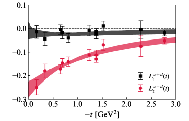
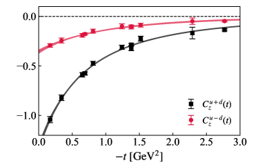
Figure 10: $L^{q}_{z}(-t)$ (left panel) and $C^{q}_{z}(-t)$ (right panel) are shown as a function of $-t$ for both the iso-vector and iso-scalar cases. The bands are derived from the dipole model fitted from the moments $\tilde{A}_{n,0}(-t)$.

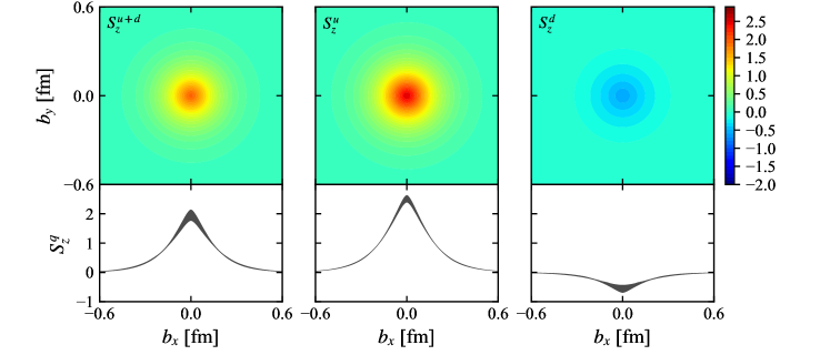
Figure 11: Upper panels: the light quark helicity density in the impact-parameter plane. Lower panels: the light quark helicity density as a function of $b_{x}$ with $b_{y}=0$, including its uncertainties.

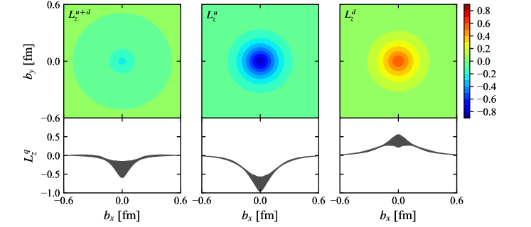
Figure 12: Upper panels: the light quark OAM density in the impact-parameter plane. Lower panels: the light quark OAM density as a function of $b_{x}$ with $b_{y}=0$, including its uncertainties.

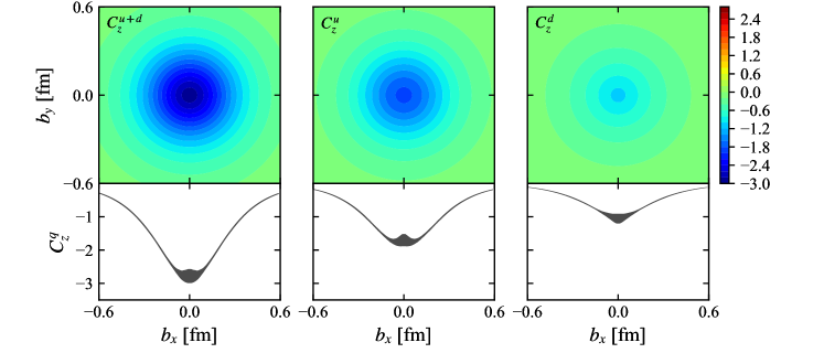
Figure 13: Upper panels: the light quark spin-orbit correlation density in the impact-parameter plane. Lower panels: the light quark spin-orbit correlation density as a function of $b_{x}$ with $b_{y}=0$, including its uncertainties.

In addition to the spin decomposition discussed above, the GPDs also provide crucial insights into the three-dimensional structure of the nucleon. By performing a Fourier transform (FT) over the momentum transfer $-t$, we can derive parton distributions in the impact-parameter space. For instance, the quark helicity distribution in this space is given by,

$$\tilde{q}(x,\mathbf{b}_{\perp})=\int\frac{{\rm d}^{2}\mathbf{\Delta}_{\perp}}{(2\pi)^{2}}\widetilde{H}(x,\xi=0,\mathbf{\Delta}^{2}_{\perp})e^{i\mathbf{b}_{\perp}\cdot\mathbf{\Delta}_{\perp}},$$ (35)

where $-t=\mathbf{\Delta}^{2}_{\perp}$. Its moments $\int_{-1}^{1}dxx^{n}\tilde{q}(x,\mathbf{b}_{\perp})$, which are the FT of the $\tilde{A}_{n+1,0}(-t)$, are averaged distributions with weight $x^{n}$ in the impact-parameter plane. In Fig. 8, we have shown the $\tilde{A}_{1,0}(-t)=2S^{q}_{z}(-t)$. Similar to Eq. (33) and Eq. (34), the quark OAM $L^{q}_{z}$ and spin-orbit correlation $C^{q}_{z}$ can also be defined with respect to momentum transfer $-t$. The results are presented in Fig. 10 for both the iso-vector and iso-scalar cases. The bands are derived using the dipole model fit from Sec. V.1 by taking the average of the results obtained from the two aforementioned fit ranges. As shown in the figures, the total light-quark OAM, $L_{z}^{u+d}$, remains small, and the amplitudes of both $L^{q}_{z}(-t)$ and $C^{q}_{z}(-t)$ decrease rapidly as $-t$ increases. For the Fourier transform over $-t$, we rely on the fit results from the dipole model, as no data is available beyond 3 $\rm GeV^{2}$. The results at small $b_{T}$ may be affected by systematic errors due to the model assumptions, though these errors are likely minimal since the moments decay quickly at large $-t$.

In Fig. 11, the quark helicity density in the impact-parameter plane is depicted. As one can see, the $u$ and $d$ quark densities have opposite signs, but the $u$ quark’s amplitude is significantly larger, resulting in a positive combined helicity contribution from $u+d$ quarks.

The quark OAM density in the impact-parameter plane, shown in Fig. 12, also exhibits opposite signs for $u$ and $d$ quarks. This suggests that $u$ and $d$ quarks orbit the longitudinal momentum in opposite directions. Notably, since the amplitudes of $u$ and $d$ quarks are similar, their sum is nearly zero. This observation is very different from the quark number density distribution we studied in Ref. Bhattacharya et al. (2023b), where the $d$ quark shows lower amplitudes in the impact-parameter space compared to the $u$ quark. This difference may imply that $d$ quarks possess a larger $k_{T}$ for a given $b_{T}$.

Lastly, for the first time, we present results for the quark spin-orbit correlation distribution in impact-parameter space. We find that these correlations are negative for both light quarks, with the $u$ quark exhibiting a larger amplitude. Interestingly, the sign of $C_{z}^{q}=\langle\textbf{S}_{z}^{q}\textbf{L}_{z}^{q}\rangle$ matches that of $S_{z}^{q}\cdot L_{z}^{q}=\langle\textbf{S}_{z}^{q}\textbf{S}_{z}^{N}\rangle\cdot\langle\textbf{L}_{z}^{q}\textbf{S}_{z}^{N}\rangle$ for each quark flavor. Additionally, unlike $S^{q}$ and $L^{q}$, which approach zero rapidly as $b_{T}$ nears the nucleon size, there is still a non-zero value observed for the spin-orbit correlation.

VI Conclusion

In this work, we present a study of the moments of axial-vector GPD $\widetilde{H}$ using lattice QCD. We compute the quasi-GPD matrix elements in an asymmetric frame with multiple values of the momentum transfer, allowing us to study the $t$ dependence. The quasi-GPDs matrix elements are then renormalized using the ratio scheme. We employ the short-distance factorization framework to extract the first few moments of the GPDs. For the first time, we obtain results for up to and including the fifth moment of axial-vector GPD $\widetilde{H}$ with reasonable signal and $t$ dependence as summarized in Table 3 and Table 4. Our determination of the first two moments is consistent with previous calculations using traditional local operator methods. From these moments we infer the quark helicity and OAM contributions to the nucleon spin as well as the quark spin-orbit correlations. In agreement with previous findings, our results indicate that the light quark helicity contributes significantly to the nucleon spin, while the OAM of individual quark flavors shows an interesting pattern of cancellation, leading to a small net OAM for the light quarks. Additionally, the spin-orbit correlations for both light quarks are found to be negative, aligning with the sign of $S^{q}_{z}\cdot L^{q}_{z}$. The magnitudes of the iso-vector and iso-scalar combinations are in agreement with the large-$N_{c}$ predictions. We emphasize that the use of an asymmetric frame with multiple values of $t$ enables us to explore impact-parameter space distributions via a Fourier transform over $t$. That provides us multiple images of the nucleon spin structure, showcasing the spatial distributions of quark helicity, orbital angular momentum (OAM) and, for the first time, the spin-orbit correlations in the transverse plane. These distributions exhibit distinct features for different quark flavors, offering a deeper understanding of the nucleon’s internal structure. However, we acknowledge several systematic uncertainties that were not addressed in this exploratory work. Future research will aim to control these uncertainties, including contributions from disconnected diagrams, quark masses at the physical point, excited-state contamination, and the continuum limit, in order to further refine our understanding of nucleon spin dynamics.

$-t~{}\rm{GeV}^{2}$	$\tilde{A}_{10}^{u-d}$	$\tilde{A}_{20}^{u-d}$	$\tilde{A}_{30}^{u-d}$	$\tilde{A}_{40}^{u-d}$	$\tilde{A}_{50}^{u-d}$
0.17	0.990(47)(01)	0.262(14)(05)	0.091(05)(01)	0.046(03)(07)	0.017(02)(02)
0.34	0.827(45)(01)	0.215(11)(06)	0.094(05)(01)	0.044(03)(08)	0.022(03)(02)
0.65	0.733(32)(01)	0.223(11)(05)	0.077(04)(01)	0.041(02)(07)	0.015(02)(02)
0.69	0.699(27)(02)	0.221(08)(05)	0.076(04)(02)	0.039(02)(06)	0.016(02)(03)
0.81	0.609(31)(01)	0.192(10)(05)	0.074(04)(01)	0.039(03)(07)	0.019(02)(02)
1.24	0.491(33)(04)	0.159(10)(04)	0.065(06)(04)	0.033(03)(06)	0.020(03)(06)
1.38	0.485(29)(02)	0.181(13)(04)	0.062(05)(02)	0.034(04)(05)	0.012(03)(03)
1.38	0.502(20)(01)	0.173(09)(03)	0.061(03)(01)	0.034(02)(04)	0.010(02)(02)
1.52	0.351(32)(02)	0.143(10)(04)	0.051(05)(02)	0.028(03)(05)	0.014(03)(03)
2.29	0.348(63)(04)	0.161(30)(04)	0.041(10)(04)	0.035(07)(05)	0.006(06)(05)
2.77	0.274(21)(02)	0.119(07)(02)	0.043(04)(02)	0.023(02)(03)	0.006(05)(02)

Table 3: The table of iso-vector moments $\tilde{A}_{n+1,0}^{u-d}$.

$-t~{}\rm{GeV}^{2}$	$\tilde{A}_{10}^{u+d}$	$\tilde{A}_{20}^{u+d}$	$\tilde{A}_{30}^{u+d}$	$\tilde{A}_{40}^{u+d}$	$\tilde{A}_{50}^{u+d}$
0.17	0.554(34)(03)	0.184(07)(05)	0.072(04)(03)	0.036(03)(06)	0.016(02)(03)
0.34	0.531(40)(02)	0.150(13)(04)	0.075(05)(02)	0.032(03)(06)	0.020(03)(03)
0.65	0.427(29)(02)	0.162(07)(04)	0.065(04)(02)	0.032(02)(06)	0.014(02)(02)
0.69	0.424(20)(01)	0.157(07)(05)	0.053(04)(01)	0.033(02)(06)	0.010(02)(01)
0.81	0.407(33)(01)	0.147(10)(04)	0.062(04)(01)	0.030(02)(06)	0.016(03)(02)
1.24	0.296(35)(02)	0.113(11)(03)	0.057(05)(02)	0.025(04)(04)	0.013(03)(03)
1.38	0.313(32)(02)	0.135(10)(03)	0.047(06)(02)	0.028(03)(04)	0.008(03)(02)
1.38	0.290(20)(01)	0.119(07)(03)	0.047(04)(01)	0.026(02)(04)	0.009(02)(02)
1.52	0.217(28)(02)	0.118(09)(03)	0.043(06)(02)	0.022(03)(04)	0.013(03)(02)
2.29	0.231(61)(04)	0.121(24)(05)	0.033(09)(04)	0.030(07)(07)	0.002(07)(05)
2.77	0.199(16)(02)	0.077(07)(03)	0.036(04)(02)	0.018(02)(03)	0.004(02)(02)

Table 4: The table of iso-scalar moments $\tilde{A}_{n+1,0}^{u+d}$.