NRGBoost: Energy-Based Generative Boosted Trees
Abstract
Despite the rise to dominance of deep learning in unstructured data domains, tree-based methods such as Random Forests (RF) and Gradient Boosted Decision Trees (GBDT) are still the workhorses for handling discriminative tasks on tabular data. We explore generative extensions of these popular algorithms with a focus on explicitly modeling the data density (up to a normalization constant), thus enabling other applications besides sampling. As our main contribution we propose an energy-based generative boosting algorithm that is analogous to the second order boosting implemented in popular packages like XGBoost. We show that, despite producing a generative model capable of handling inference tasks over any input variable, our proposed algorithm can achieve similar discriminative performance to GBDT on a number of real world tabular datasets, outperforming alternative generative approaches. At the same time, we show that it is also competitive with neural network based models for sampling.
1 Introduction
Generative models have achieved tremendous success in computer vision and natural language processing, where the ability to generate synthetic data guided by user prompts opens up many exciting possibilities. While generating synthetic table records does not necessarily enjoy the same wide appeal, this problem has still received considerable attention as a potential avenue for bypassing privacy concerns when sharing data. Estimating the data density, , is another typical application of generative models which enables a host of different use cases that can be particularly interesting for tabular data. Unlike discriminative models which are trained to perform inference over a single target variable, density models can be used more flexibly for inference over different variables or for out of distribution detection. They can also handle inference with missing data in a principled way by marginalizing over unobserved variables.
The development of generative models for tabular data has mirrored its progression in computer vision with many of its Deep Learning (DL) approaches being adapted to the tabular domain (Jordon et al., 2018; Xu et al., 2019; Fan et al., 2020; Engelmann & Lessmann, 2021; Zhao et al., 2021; Kotelnikov et al., 2023). Unfortunately, these methods are only useful for sampling as they either don’t model the density explicitly or can’t evaluate it due to untractable marginalization over high dimensional latent variable spaces. Furthermore, despite growing in popularity, DL has still failed to displace tree-based ensemble methods as the tool of choice for handling tabular discriminative tasks with gradient boosting still being found to outperform neural-network-based methods in many real world datasets (Grinsztajn et al., 2022; Borisov et al., 2022a).
While there have been recent efforts to extend the success of tree-based models to generative modeling (Correia et al., 2020; Wen & Hang, 2022; Nock & Guillame-Bert, 2022; Watson et al., 2023; Nock & Guillame-Bert, 2023; Jolicoeur-Martineau et al., 2024), direct extensions of Random Forests (RF) and Gradient Boosted Decision Trees (GBDT) are still missing. It is this gap that we try to address, seeking to keep the general algorithmic structure of these popular algorithms but replacing the optimization of their discriminative objective with a generative counterpart. Our main contributions in this regard are:
-
•
We propose NRGBoost, a novel energy-based generative boosting model that is trained to maximize a local second order approximation to the likelihood at each boosting round.
-
•
We propose an amortized sampling approach that greatly reduces the training time of NRGBoost, which, like other energy-based models, is often dominated by sampling.
-
•
We explore the use of bagged ensembles of Density Estimation Trees (DET) (Ram & Gray, 2011) with feature subsampling as a generative counterpart to Random Forests.
The longstanding popularity of GBDT models in machine learning practice can, in part, be attributed to the strength of its empirical results and the efficiency of its existing implementations. We therefore focus on an experimental evaluation in real world datasets spanning a range of use cases, number of samples and features. On smaller datasets, our implementation of NRGBoost can be trained in a few minutes on a mid-range consumer CPU and achieves similar discriminative performance to a standard GBDT model, while remaining competitive with the best generative models for sampling.
2 Energy Based Models
An Energy-Based Model (EBM) parametrizes the logarithm of a probability density function directly (up to an unspecified normalizing constant):
| (1) |
Here is a real function over the input domain.111 We will assume that is finite and discrete to simplify the notation and exposition but everything is applicable to bounded continuous input spaces, replacing the sums with integrals as appropriate. We will avoid introducing any parametrization, instead treating the function lying in an appropriate function space over the input space as our model parameter directly. , known as the partition function, is then a functional of giving us the necessary normalizing constant.
This is the most flexible way one could represent a probability density function making essentially no compromises on its structure. The downside to this is that for most interesting choices of , computing or estimating this normalizing constant is untractable which makes training these models difficult. Their unnormalized nature, however, does not prevent EBMs from being useful in a number of applications besides sampling. They can be used to perform inference over small enough groups of variables. Partitioning the input space into a set of observed variables and unobserved variables we have
| (2) |
which only involves normalizing (i.e., computing a softmax) over the possible values of the unobserved variables. Furthermore, for anomaly or out of distribution detection, knowledge of the normalizing constant is not necessary.
One common way to train an energy-based model to approximate a data generating distribution, , is to minimize the Kullback-Leibler divergence between and , or equivalently, maximize the expected log likelihood functional:
| (3) |
This optimization is typically carried out by gradient descent over the parameters of , but due to the intractability of the partition function, one must rely on Markov Chain Monte Carlo (MCMC) sampling to estimate the gradients (Song & Kingma, 2021).
3 NRGBoost
Expanding the increase in log-likelihood in equation 3 due to a variation around an energy function up to second order we have
| (4) |
The that maximizes this quadratic approximation should thus have a large positive difference between the expected value under the data and under while having low variance under . We note that just like the original log-likelihood, this Taylor expansion is invariant to adding an overall constant to . This means that, in maximizing equation 4 we can consider only functions that have zero expectation under in which case we can simplify as
| (5) |
We thus formulate our boosting algorithm as modelling the data density with an additive energy function. At each boosting iteration we improve upon the current energy function by finding an optimal step that maximizes :
| (6) |
where is an appropriate space of functions (satisfying if equation 5 is used). The solution to this problem can be interpreted as a Newton step in the space of energy functions. Because for an EBM, the Fisher Information matrix with respect to the energy function and the hessian of the expected log-likelihood are the same (see Appendix A), we can also interpret the solution to equation 6 as a natural gradient step. This approach is analogous to the second order step implemented in modern gradient boosting libraries such as XGBoost (Chen & Guestrin, 2016) and LightGBM (Ke et al., 2017) and which can be traced back to Friedman et al. (2000).
In updating the current iterate, , we scale by an additional scalar step-size . This can be interpreted as a globalization strategy to account for the fact that the quadratic approximation in equation 4 is not necessarily valid over large steps in function space. A common strategy in nonlinear optimization would be to select via a line search based on the original log-likelihood. Common practice in discriminative boosting however is to interpret this step size as a regularization parameter and to select a fixed value in with (more) smaller steps typically outperforming fewer larger ones when it comes to generalization. We choose to adopt a hybrid strategy, first selecting an optimal step size by line search and then shrinking it by a fixed factor. We find that this typically accelerates convergence allowing the algorithm to take comparatively larger steps that increase the likelihood in the initial phase of boosting.
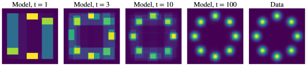
For a starting point, , we can choose the logarithm of any probability distribution over as long as it is easy to evaluate. Sensible choices are a uniform distribution (i.e., ), the product of marginals for the training set, or any mixture distribution between these two. In Figure 2 we show an example of NRGBoost starting from a uniform distribution and learning a toy 2D data density.
3.1 Weak Learners
As a weak learner we will consider piecewise constant functions defined by binary trees over the input space. Letting be the partitioning of the input space induced by the leaves of a binary tree whose internal nodes represent a split along one dimension into two disjoint partitions, we take as the set of functions such as
| (7) |
where denotes the indicator function of a subset and are values associated with each leaf . In a standard decision tree these values would typically encode an estimate of , with being a special target variable that is never considered for splitting. In our generative approach they encode unconditional densities (or more precisely energies) over each leaf’s support and every variable can be used for splitting. Note that our functions are thus parametrized by the values as well the structure of the tree and the variables and values for the split at each node which ultimately determine the . We omit these dependencies for brevity.
Replacing the definition in equation 7 in our objective (equation 5) we get the following optimization problem to find the optimal decision tree:
| (8) | ||||
| s.t. |
where and denote the probability of the event under the respective distribution and the constraint ensures that has zero expectation under . With respect to the leaf weights this is a quadratic program whose optimal solution and objective values are respectively given by
| (9) |
Because carrying out the maximization of this optimal value over the tree structure that determines the is hard, we approximate its solution by greedily growing a tree that maximizes it when considering how to split each node individually. A parent leaf with support is thus split into two child leaves, with disjoint support, , so as to maximize over all possible partitionings along a single dimension, , the following objective:
| (10) |
Note that, when using parametric weak learners, computing a second order step would typically involve solving a linear system with a full Hessian. As we can see, this is not the case when the weak learners are decision trees, where the optimal value to assign to a leaf does not depend on any information from other leaves and, likewise, the optimal objective value is a sum of terms, each depending only on information from a single leaf. This would have not been the case had we tried to optimize the likelihood functional in Equation 3 directly instead of its quadratic approximation.
3.2 Amortized Sampling
To compute the leaf values in equation 9 and the splitting criterion in equation 10 we would have to know and be able to compute which is infeasible due to the untractable normalization constant. We therefore estimate these quantities, with recourse to empirical data for , and to samples approximately drawn from the model with MCMC. Because even if the input space is not partially discrete, is still discontinuous and constant almost everywhere we can’t use gradient based samplers and therefore rely on Gibbs sampling instead. This only requires evaluating each along one dimension at a time, while keeping all others fixed which can be computed efficiently for a tree by traversing it only once. However, since at boosting iteration our energy function is a sum of trees, this computation scales linearly with the iteration number. This makes the overall time spent sampling quadratic in the number of boosting iterations and thus precluding us from training models with a large number of trees.
In order to reduce the burden associated with this sampling, which dominates the runtime of training the model, we propose a new sampling approach that leverages the cumulative nature of boosting. The intuition behind this approach is that the set of samples used in the previous boosting round are (approximately) drawn from a distribution that is already close to the new model distribution. It could therefore be helpful to keep some of those samples, especially those that conform the best to the new model. Rejection sampling allows us to do just that. The boosting update in terms of the densities takes the following multiplicative form:
| (11) |
Here, is an unknown multiplicative constant and since is given by a tree, we can easily bound the exponential factor by finding the leaf with the largest value. We can therefore use the previous model, , as a proposal distribution for which we already have a set of samples and keep each sample, , with an acceptance probability of:
| (12) |
We note that knowledge of the constant is not necessary to compute this probability.
Our proposed sampling strategy is to maintain a fixed size pool of approximate samples from the model. At the end of each boosting round, we use rejection sampling to remove samples from the pool and draw new samples from the model using Gibbs sampling. Note that is typically a simple model for which we can both directly evaluate the desired quantities (i.e., for a given partition ) and cheaply draw exact samples from. As such, no samples are required for the first iteration of boosting and for the second we can initialize the sample pool by drawing exact samples from with rejection sampling using as a proposal distribution.
This approach works better when the range of and/or the step sizes are small as this leads to larger acceptance probabilities. Note that in practice it can be helpful to independently refresh a fixed fraction of samples, , at each round of boosting in order to encourage more diverse samples between rounds. This can be accomplished by keeping each sample with a probability instead.
3.3 Regularization
The simplest way to regularize a boosting model is to stop training when overfitting is detected by monitoring a suitable performance metric on a validation set. For NRGBoost this could be the increase in log-likelihood at each boosting round. However, estimating this quantity would require drawing additional validation samples from the model (see Appendix A.1). An alternative viable validation strategy which needs no additional samples is to simply monitor a discriminative performance metric. This amounts to monitoring the quality of instead of the full .
Besides early stopping, the decision trees themselves can be regularized by limiting the depth or total number of leaves in each tree. Additionally, we can rely on other strategies such as disregarding splits that would result in a leaf with too little training data, , model data, , volume or too high of a ratio between training and model data . We found the latter to be the most effective of these, not only yielding better generalization performance than other approaches, but also having the added benefit of allowing us to lower bound the acceptance probability of our rejection sampling scheme. Furthermore, as we show in Appendix A.2, limiting this ratio guarantees that a small enough step size produces an increase in likelihood at each round of boosting.
4 Density Estimation Trees and Density Estimation Forests
Density Estimation Trees (DET) were proposed by Ram & Gray (2011) as an alternative to histograms and kernel density estimation but have received little attention as generative models for sampling or other applications. They model the density function as a constant value over the support of each leaf in a binary tree,
| (13) |
with being an empirical estimate of probability of the event and denoting the volume of . Note that it is possible to draw an exact sample from this type of model by randomly selecting a leaf, , given probabilities , and then drawing a sample from a uniform distribution over .
To fit a DET, Ram & Gray (2011) propose optimizing the Integrated Squared Error (ISE) between the data and model distributions which, following a similar approach to Section 3.1, leads the following optimization problem when considering how to split a leaf node:
| (14) |
For the ISE, should be taken as the function which leads to a similar splitting criterion to Equation 14 but replacing the previous model’s distribution with the volume measure which can be interpreted as the uniform distribution on (up to a multiplicative constant).
Maximum Likelihood
Often generative models are trained to maximize the likelihood of the observed data. This was left for future work in Ram & Gray (2011) but, as we show in Appendix B, can be accomplished by replacing with . This choice of minimization criterion can be seen as analogous to the choice between Gini impurity and Shannon entropy in the computation of the information gain in decision trees.
Bagging and Feature Subsampling
Following the common approach in decision trees, Ram & Gray (2011) suggest the use of pruning for regularization of DET models. Practice has however evolved to prefer bagging as a form of regularization rather than relying on single decision trees. We employ same principle to DETs by fitting many trees on bootstrap samples of the data. We also adopt the common practice from Random Forests of randomly sampling a subset of features to consider when splitting any leaf node in order to encourage independence between the different trees in the ensemble. The ensemble model, which we call Density Estimation Forests (DEF) in the sequel, is thus an additive mixture of DETs with uniform weights, therefore still allowing for normalized density computation and exact sampling.
5 Related Work
Generative Boosting
Most prior work on generative boosting focuses on unstructured data and the use of parametric weak learners and is split between two approaches: (i) Additive methods that model the density function as an additive mixture of weak learners such as Rosset & Segal (2002); Tolstikhin et al. (2017). (ii) Those that take a multiplicative approach modeling the density function as an unnormalized product of weak learners. The latter is equivalent to the energy based approach that writes the energy function (log density) as an additive sum of weak learners. Welling et al. (2002) in particular also approach boosting from the point of view of functional optimization of the likelihood or the logistic loss of an energy-based model. However, they rely on a first order local approximation of the objective since they focus on parametric weak learners such as restricted Boltzmann machines for which a second order step would be impractical.
Greedy Multiplicative Boosting
Another more direct multiplicative boosting framework was first proposed by Tu (2007). At each boosting round a discriminative classifier is trained to distinguish between empirical data and data generated by the current model by estimating the likelihood ratio . This estimated ratio is used as a direct multiplicative factor to update the current model (after being raised to an appropriate step size). In ideal conditions this greedy procedure would converge in a single iteration if a step size of 1 would be used. While Tu (2007) does not prescribe a particular choice of classifier, Grover & Ermon (2018) proposes a similar concept where the ratio is estimated based on an adversarial bound for an -divergence and Cranko & Nock (2019) provides additional analysis on this method. We note that the main difference between this greedy approach and NRGBoost is that the latter attempts to update the current density proportionally to an exponential of the likelihood ratio, , instead of directly. In Appendix C we explore the differences between NRGBoost and this approach when it is adapted to use trees as weak learners.
Tree-Based Density Modelling
Other authors have proposed tree-based density models similar to DET (Nock & Guillame-Bert, 2022) or additive mixtures of tree-based models (Correia et al., 2020; Wen & Hang, 2022; Watson et al., 2023) but perhaps surprisingly, the natural idea of creating an ensemble of DET models through bagging has not been explored before as far as we are aware. Distinguishing features of some of these alternative approaches are: (i) Not relying on a density estimation goal to drive the partitioning of the input space. Correia et al. (2020) leverages a standard discriminative Random Forest, therefore giving special treatment to a particular input variable whose conditional estimation drives the choice of partitions and Wen & Hang (2022) proposes using a mid-point random tree partitioning. (ii) Leveraging more complex models for the data in the leaf of a tree instead of a uniform density (Correia et al., 2020; Watson et al., 2023). This can allow for the use of trees that are more representative with a smaller number of leaves. (iii) Relying on an adversarial framework where the generator and discriminator are both a tree (Nock & Guillame-Bert, 2022) or an ensemble of trees (Watson et al., 2023). While this also leads to an iterative approach, unlike with boosting or bagging, the new model trained at each round doesn’t add to the previous one but replaces it instead.
Other Recent Tree-Based approaches
Nock & Guillame-Bert (2023) proposes a different ensemble approach where each tree does not have its own leaf values that get added or multiplied to produce the final density, but instead serve to collectively define the partitioning of the input space. To train such models the authors propose a framework where, rather than adding a new tree to the ensemble at every iteration, the model is initialized with a fixed number of tree root nodes and each iteration adds a split to an existing leaf node. Finally Jolicoeur-Martineau et al. (2024) propose a diffusion model where a tree-based model (e.g., GBDT) is used to regress the score function. Being a diffusion model, however, means that computing densities is untractable.
6 Experiments
We evaluate the our proposed methods on 5 tabular datasets from the UCI Machine Learning Repository (Dheeru & Karra Taniskidou, 2017): Abalone (AB), Physicochemical Properties of Protein Tertiary Structure (PR), Adult (AD), MiniBooNE (MBNE) and Covertype (CT) as well as the California Housing (CH) dataset available through scikit-learn (Pedregosa et al., 2011). We also include a downsampled version of MNIST (by 2x along each dimension) which allows us to visually assess the quality of individual samples, something that is generally difficult with structured tabular data. More details about these datasets are given in Appendix D.1.
We split our experiments into two sections, the first to evaluate the quality of density models directly on a single variable inference task and the second to investigate the performance of our proposed models when used for sampling, comparing them against more specialized models.
6.1 Single Variable Inference
We test the ability of a generative model, trained to learn the density over all input variables, , to infer the value of a single one (i.e., we evaluate the quality of its estimate of ). For this purpose we pick as the original target of the dataset, noting that the models that we train do not treat this variable in any special way, except for the selection of the best model in validation. As such, we would expect that the model’s performance in inference over this particular variable is indicative of its strength on any other single variable inference task and also indicative of the quality of the full from which the conditional probability estimate is derived.
We use XGBoost (Chen & Guestrin, 2016) as a baseline for what should be achievable by a strong discriminative model, noting that it is trained to maximize the discriminative likelihood, , directly, not wasting model capacity in learning other aspects of the full data distribution. We also compare to two other tree-based generative baselines: RFDE (Wen & Hang, 2022) and ARF (FORDE) (Watson et al., 2023). The former allows us to gauge the impact of the guided partitioning used in DEF models over a random partitioning of the input space.
We use random search to tune the hyperparameters of the XGBoost model and a grid search to tune the most important hyperparameters of each generative density model. We employ 5-fold cross-validation, repeating the hyperparameter tuning on each fold. For the full details of the experimental protocol please refer to Appendix D.
| AUC | Accuracy | ||||||
| AB | CH | PR | AD | MBNE | MNIST | CT | |
| XGBoost | 0.552 ±0.035 | 0.849 ±0.009 | 0.678 ±0.004 | 0.927 ±0.000 | 0.987 ±0.000 | 0.976 ±0.002 | 0.971 ±0.001 |
| RFDE | 0.071 ±0.096 | 0.340 ±0.004 | 0.059 ±0.007 | 0.862 ±0.002 | 0.668 ±0.008 | 0.302 ±0.010 | 0.679 ±0.002 |
| ARF | 0.531 ±0.032 | 0.758 ±0.009 | 0.591 ±0.007 | 0.893 ±0.002 | 0.968 ±0.001 | -∗ | 0.938 ±0.005 |
| DEF (ISE) | 0.467 ±0.037 | 0.737 ±0.008 | 0.566 ±0.002 | 0.854 ±0.003 | 0.653 ±0.011 | 0.206 ±0.011 | 0.790 ±0.003 |
| DEF (KL) | 0.482 ±0.027 | 0.801 ±0.008 | 0.639 ±0.004 | 0.892 ±0.001 | 0.939 ±0.001 | 0.487 ±0.007 | 0.852 ±0.002 |
| NRGBoost | 0.547 ±0.036 | 0.850 ±0.011 | 0.676 ±0.009 | 0.920 ±0.001 | 0.974 ±0.001 | 0.966 ±0.001 | 0.948 ±0.001 |
-
•
∗ Due to the discrete nature of the MNIST dataset and the fact that the ARF algorithm tries to fit continuous distributions at the leaves, we could not obtain a reasonable density model for this dataset.
We find that NRGBoost outperforms the remaining generative models (see Table 1), even achieving comparable performance to XGBoost on the smaller datasets and with a small gap on the three larger ones (MBNE, MNIST, CT). We note also that for the regression datasets, the generative models provide an estimate of the full conditional distribution over the target variable rather than a point estimate like XGBoost. While there are other variants of boosting that can do the same (Duan et al., 2020), they rely on a parametric assumption about that needs to hold for any .
6.2 Sampling
We evaluate two different aspects of the quality of generated samples: their utility for training a machine learning model and how distinguishable they are from real data.
Besides ARF, we compare to TVAE (Xu et al., 2019) and TabDDPM (Kotelnikov et al., 2023), two neural-network based generative models, as well as Forest-Flow (Jolicoeur-Martineau et al., 2024), a tree-based diffusion model. Note that these three methods are not capable of density estimation.
Machine Learning Efficiency
Machine learning (ML) efficiency has been a popular way to measure the quality of generative models for sampling (Xu et al., 2019; Borisov et al., 2022b; Kotelnikov et al., 2023). It relies on using samples from a generative model to train a discriminative model which is then evaluated on real data, and is thus similar to the single variable inference performance that we use to compare density models in Section 6.1. In fact, if the density model’s support covers that of the full data, one would expect the discriminative model to recover the generator’s , and therefore its performance, in the limit where infinite generated data is used to train it.
We use an XGBoost model as the discriminative model and train it on the same number of training samples as the original data. For the density models, we generate samples from the best model found in the previous section and for TVAE and TabDDM we select their hyperparameters by evaluating the ML Efficiency in the real validation set (full details of the hyperparameter tuning are provided in Appendix D.2). Note that this leaves these models at a potential advantage since the hyperparameter selection is based on the metric that is being evaluated.
We repeat all experiments 5 times, with different generated datatsets from each model and report the performance of the discriminative model in Table 2. We find that NRGBoost and TabDDPM alternate as the best-performing model depending on the dataset (with two inconclusive cases), and NRGBoost is never ranked lower than second on any dataset. We note also that, despite our best efforts with additional manual tuning, we could not achieve a reasonable model with TabDDM on MNIST.
| AUC | Accuracy | ||||||
| AB | CH | PR | AD | MBNE | MNIST | CT | |
| Real Data | 0.554 | 0.838 | 0.682 | 0.927 | 0.987 | 0.976 | 0.972 |
| TVAE | 0.483 ±0.006 | 0.758 ±0.005 | 0.365 ±0.005 | 0.898 ±0.001 | 0.975 ±0.000 | 0.770 ±0.009 | 0.750 ±0.002 |
| TabDDPM | 0.539 ±0.018 | 0.807 ±0.005 | 0.596 ±0.007 | 0.910 ±0.001 | 0.984 ±0.000 | - | 0.818 ±0.001 |
| Forest-Flow | 0.418 ±0.019 | 0.716 ±0.003 | 0.412 ±0.009 | 0.879 ±0.003 | 0.964 ±0.001 | 0.224 ±0.010 | 0.705 ±0.002 |
| ARF | 0.504 ±0.020 | 0.739 ±0.003 | 0.524 ±0.003 | 0.901 ±0.001 | 0.971 ±0.001 | 0.908 ±0.002 | 0.848 ±0.002 |
| DEF (KL) | 0.450 ±0.013 | 0.762 ±0.006 | 0.498 ±0.007 | 0.892 ±0.001 | 0.943 ±0.002 | 0.230 ±0.028 | 0.753 ±0.002 |
| NRGBoost | 0.528 ±0.016 | 0.801 ±0.001 | 0.573 ±0.008 | 0.914 ±0.001 | 0.977 ±0.001 | 0.959 ±0.001 | 0.895 ±0.001 |
Discriminator Measure
Similar to Borisov et al. (2022b) we test the capacity of a discriminative model to distinguish between real and generated data. We use the original validation set as the real part of the training data for the discriminator in order to avoid benefiting generative methods that overfit their original training set. A new validation set is carved out of the original test set (20%) and used to tune the hyperparameters of an XGBoost model which we use as our discriminator. We report the AUC of this model on the remainder of the real test data in Table 3 which shows that NRGBoost outperforms other methods except on the PR (with an inconclusive result) and MBNE datasets.
| AB | CH | PR | AD | MBNE | MNIST | CT | |
| TVAE | 0.971 ±0.004 | 0.834 ±0.006 | 0.940 ±0.002 | 0.898 ±0.001 | 1.000 ±0.000 | 1.000 ±0.000 | 0.999 ±0.000 |
| TabDDPM | 0.818 ±0.015 | 0.667 ±0.005 | 0.628 ±0.004 | 0.604 ±0.002 | 0.789 ±0.002 | - | 0.915 ±0.007 |
| Forest-Flow | 0.987 ±0.002 | 0.926 ±0.002 | 0.885 ±0.002 | 0.932 ±0.002 | 1.000 ±0.000 | 1.000 ±0.000 | 0.985 ±0.001 |
| ARF | 0.975 ±0.005 | 0.973 ±0.004 | 0.795 ±0.008 | 0.992 ±0.000 | 0.998 ±0.000 | 1.000 ±0.000 | 0.989 ±0.001 |
| DEF (KL) | 0.823 ±0.013 | 0.751 ±0.008 | 0.877 ±0.002 | 0.956 ±0.002 | 1.000 ±0.000 | 1.000 ±0.000 | 0.999 ±0.000 |
| NRGBoost | 0.625 ±0.017 | 0.574 ±0.012 | 0.631 ±0.006 | 0.559 ±0.003 | 0.993 ±0.001 | 0.943 ±0.003 | 0.724 ±0.006 |
Statistical Distance Measure
As an additional measure of the statistical dissimilarity between data and model distributions we evaluate a Wasserstein distance using a similar setup to Jolicoeur-Martineau et al. (2024). Namely, we min-max scale the numerical variables, and one-hot encode the categorical variables and scale them by 1/2. We use a distance in the formulation of the optimal transport problem. Since finding the optimal solution has a worst case cubic scaling with the sample size, we sub-sample a maximum of 5000 samples from the original train or test sets and use an equal number of synthetic samples. We repeat the evaluation for each method and dataset 5 times using different synthetic data and also different subsampling seeds for the real data (where applicable).
| AB | CH | PR | AD | MBNE | MNIST | CT | |
| TVAE | 0.302 ±0.005 | 0.206 ±0.010 | 0.274 ±0.008 | 1.086 ±0.023 | 0.425 ±0.032 | 20.61 ±0.042 | 0.807 ±0.023 |
| TabDDPM | 0.500 ±0.023 | 0.169 ±0.009 | 0.195 ±0.003 | 0.938 ±0.029 | 109.5 ±93.13 | - | 0.646 ±0.022 |
| Forest-Flow | 0.248 ±0.020 | 0.205 ±0.009 | 0.231 ±0.008 | 1.243 ±0.029 | 4.295 ±3.697 | 20.73 ±0.574 | 0.893 ±0.021 |
| ARF | 0.218 ±0.015 | 0.240 ±0.009 | 0.238 ±0.006 | 1.378 ±0.020 | 0.732 ±0.664 | 18.14 ±0.060 | 0.709 ±0.018 |
| DEF (KL) | 0.337 ±0.006 | 0.210 ±0.012 | 0.264 ±0.011 | 1.696 ±0.023 | 18.29 ±14.90 | 261.0 ±35.01 | 0.935 ±0.024 |
| NRGBoost | 0.502 ±0.045 | 0.178 ±0.011 | 0.225 ±0.010 | 1.051 ±0.013 | 22.33 ±20.11 | 15.70 ±0.188 | 0.602 ±0.015 |
| AB | CH | PR | AD | MBNE | MNIST | CT | |
| TVAE | 0.299 ±0.005 | 0.195 ±0.010 | 0.274 ±0.011 | 1.075 ±0.024 | 0.366 ±0.055 | 20.59 ±0.041 | 0.808 ±0.029 |
| TabDDPM | 0.467 ±0.021 | 0.153 ±0.007 | 0.190 ±0.005 | 0.895 ±0.019 | 109.6 ±93.14 | - | 0.640 ±0.016 |
| Forest-Flow | 0.234 ±0.020 | 0.192 ±0.007 | 0.238 ±0.009 | 1.239 ±0.024 | 4.214 ±3.683 | 20.73 ±0.574 | 0.896 ±0.022 |
| ARF | 0.199 ±0.015 | 0.233 ±0.009 | 0.232 ±0.007 | 1.363 ±0.018 | 0.698 ±0.684 | 18.14 ±0.060 | 0.703 ±0.019 |
| DEF (KL) | 0.320 ±0.006 | 0.199 ±0.012 | 0.260 ±0.010 | 1.682 ±0.024 | 18.21 ±14.92 | 261.0 ±15.60 | 0.933 ±0.025 |
| NRGBoost | 0.509 ±0.047 | 0.170 ±0.012 | 0.230 ±0.011 | 1.028 ±0.015 | 22.25 ±20.09 | 15.60 ±0.212 | 0.600 ±0.016 |
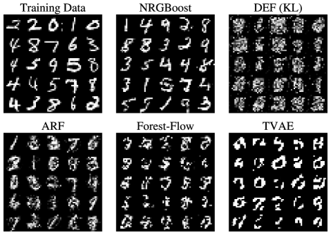
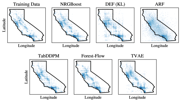
Our results for the distance between empirical training and test distribution and synthetic samples from each model are reported in Tables 5 and 4 respectively. We found these results to be somewhat sensitive to the choice of normalization of the numericals and categoricals, as well as to the choice of distance in this normalized space. Despite NRGBoost not being as dominant as in the discriminator measure, it still fares well, obtaining the best average rank over all datasets and experiments. Qualitatively speaking, we find that the samples generated by NRGBoost also look visually similar to the real data in both the MNIST and California datasets (see Figures 1 and 3), being the only generative model that can claim that for the former.
7 Discussion
The proposed DEF models are easy to sample from and require no sampling during training. However, we find that, they require deep trees to model the data well which, in turn, also requires a larger number of trees in the ensemble to regularize. In our experiments we found that the performance of DEF models was often capped by the maximum number of leaves we allowed ().
In contrast, NRGBoost was able to model the data better while using shallower trees and in fewer number (the models selected on all datasets except for MNIST and CT had leaves). Its main downside is that it can only be sampled from approximately using more expensive MCMC and also requires sampling during the training process. While our fast Gibbs sampling implementation and our proposed sampling approach were able to mitigate the slow training, making these models practical, they can still be cumbersome to use for sampling, particularly if independent samples are required, due to autocorrelation between samples from the same Markov Chain. We argue however that unlike in image or text generation where fast sampling is necessary for an interactive user experience, this can be less of a concern for the task of generating synthetic datasets where the one time cost of sampling is not as important as faithfully capturing the data generating distribution.
A limitation of tree-based models when compared to DL approaches is that they require keeping the full training data in memory. While discretization allows this data to be stored in a compact format, this could still limit the applicability of these methods to very large datasets.
8 Conclusion
We extend the two most popular tree-based discriminative methods for use in generative modeling. We find that our boosting approach, in particular, offers generally good discriminative performance and competitive sampling performance to more specialized alternatives. We hope that these results encourage further research into generative boosting approaches for tabular data, in particular exploring other applications besides sampling that are enabled by (unnormalized) density models.
References
- Blesch & Wright (2023) Kristin Blesch and Marvin N Wright. arfpy: A python package for density estimation and generative modeling with adversarial random forests. arXiv preprint arXiv:2311.07366, 2023.
- Borisov et al. (2022a) Vadim Borisov, Tobias Leemann, Kathrin Seßler, Johannes Haug, Martin Pawelczyk, and Gjergji Kasneci. Deep neural networks and tabular data: A survey. IEEE transactions on neural networks and learning systems, 2022a.
- Borisov et al. (2022b) Vadim Borisov, Kathrin Seßler, Tobias Leemann, Martin Pawelczyk, and Gjergji Kasneci. Language models are realistic tabular data generators. arXiv preprint arXiv:2210.06280, 2022b.
- Chen & Guestrin (2016) Tianqi Chen and Carlos Guestrin. XGBoost: A Scalable Tree Boosting System. In Proceedings of the 22nd ACM SIGKDD International Conference on Knowledge Discovery and Data Mining, pp. 785–794, August 2016. doi: 10.1145/2939672.2939785. arXiv:1603.02754 [cs].
- Correia et al. (2020) Alvaro Correia, Robert Peharz, and Cassio P de Campos. Joints in random forests. In H. Larochelle, M. Ranzato, R. Hadsell, M.F. Balcan, and H. Lin (eds.), Advances in Neural Information Processing Systems, volume 33, pp. 11404–11415. Curran Associates, Inc., 2020.
- Cranko & Nock (2019) Zac Cranko and Richard Nock. Boosted Density Estimation Remastered. In Proceedings of the 36th International Conference on Machine Learning, pp. 1416–1425. PMLR, May 2019. ISSN: 2640-3498.
- Deng (2012) Li Deng. The mnist database of handwritten digit images for machine learning research. IEEE Signal Processing Magazine, 29(6):141–142, 2012.
- Dheeru & Karra Taniskidou (2017) Dua Dheeru and Efi Karra Taniskidou. UCI machine learning repository, 2017.
- Duan et al. (2020) Tony Duan, Avati Anand, Daisy Yi Ding, Khanh K Thai, Sanjay Basu, Andrew Ng, and Alejandro Schuler. Ngboost: Natural gradient boosting for probabilistic prediction. In International conference on machine learning, pp. 2690–2700. PMLR, 2020.
- Engelmann & Lessmann (2021) Justin Engelmann and Stefan Lessmann. Conditional wasserstein gan-based oversampling of tabular data for imbalanced learning. Expert Systems with Applications, 174:114582, 2021.
- Fan et al. (2020) Ju Fan, Junyou Chen, Tongyu Liu, Yuwei Shen, Guoliang Li, and Xiaoyong Du. Relational data synthesis using generative adversarial networks: a design space exploration. Proceedings of the VLDB Endowment, 13(12):1962–1975, August 2020. ISSN 2150-8097. doi: 10.14778/3407790.3407802.
- Friedman et al. (2000) Jerome Friedman, Trevor Hastie, and Robert Tibshirani. Additive logistic regression: a statistical view of boosting (With discussion and a rejoinder by the authors). The Annals of Statistics, 28(2):337–407, April 2000. ISSN 0090-5364, 2168-8966. doi: 10.1214/aos/1016218223. Publisher: Institute of Mathematical Statistics.
- Grinsztajn et al. (2022) Léo Grinsztajn, Edouard Oyallon, and Gaël Varoquaux. Why do tree-based models still outperform deep learning on typical tabular data? Advances in neural information processing systems, 35:507–520, 2022.
- Grover & Ermon (2018) Aditya Grover and Stefano Ermon. Boosted generative models. In Proceedings of the AAAI Conference on Artificial Intelligence, volume 32, 2018.
- Harris et al. (2020) Charles R. Harris, K. Jarrod Millman, Stéfan J. van der Walt, Ralf Gommers, Pauli Virtanen, David Cournapeau, Eric Wieser, Julian Taylor, Sebastian Berg, Nathaniel J. Smith, Robert Kern, Matti Picus, Stephan Hoyer, Marten H. van Kerkwijk, Matthew Brett, Allan Haldane, Jaime Fernández del Río, Mark Wiebe, Pearu Peterson, Pierre Gérard-Marchant, Kevin Sheppard, Tyler Reddy, Warren Weckesser, Hameer Abbasi, Christoph Gohlke, and Travis E. Oliphant. Array programming with NumPy. Nature, 585(7825):357–362, September 2020. doi: 10.1038/s41586-020-2649-2.
- Jolicoeur-Martineau et al. (2024) Alexia Jolicoeur-Martineau, Kilian Fatras, and Tal Kachman. Generating and imputing tabular data via diffusion and flow-based gradient-boosted trees. In International Conference on Artificial Intelligence and Statistics, pp. 1288–1296. PMLR, 2024.
- Jordon et al. (2018) James Jordon, Jinsung Yoon, and Mihaela Van Der Schaar. Pate-gan: Generating synthetic data with differential privacy guarantees. In International conference on learning representations, 2018.
- Ke et al. (2017) Guolin Ke, Qi Meng, Thomas Finley, Taifeng Wang, Wei Chen, Weidong Ma, Qiwei Ye, and Tie-Yan Liu. LightGBM: A Highly Efficient Gradient Boosting Decision Tree. In Advances in Neural Information Processing Systems, volume 30. Curran Associates, Inc., 2017.
- Kotelnikov et al. (2023) Akim Kotelnikov, Dmitry Baranchuk, Ivan Rubachev, and Artem Babenko. Tabddpm: Modelling tabular data with diffusion models. In International Conference on Machine Learning, pp. 17564–17579. PMLR, 2023.
- Nock & Guillame-Bert (2022) Richard Nock and Mathieu Guillame-Bert. Generative trees: Adversarial and copycat. In Kamalika Chaudhuri, Stefanie Jegelka, Le Song, Csaba Szepesvari, Gang Niu, and Sivan Sabato (eds.), Proceedings of the 39th International Conference on Machine Learning, volume 162 of Proceedings of Machine Learning Research, pp. 16906–16951. PMLR, 17–23 Jul 2022.
- Nock & Guillame-Bert (2023) Richard Nock and Mathieu Guillame-Bert. Generative forests. arXiv preprint arXiv:2308.03648, 2023.
- O’Neill (2014) Melissa E. O’Neill. Pcg: A family of simple fast space-efficient statistically good algorithms for random number generation. Technical Report HMC-CS-2014-0905, Harvey Mudd College, Claremont, CA, September 2014.
- Pedregosa et al. (2011) F. Pedregosa, G. Varoquaux, A. Gramfort, V. Michel, B. Thirion, O. Grisel, M. Blondel, P. Prettenhofer, R. Weiss, V. Dubourg, J. Vanderplas, A. Passos, D. Cournapeau, M. Brucher, M. Perrot, and E. Duchesnay. Scikit-learn: Machine learning in Python. Journal of Machine Learning Research, 12:2825–2830, 2011.
- Ram & Gray (2011) Parikshit Ram and Alexander G. Gray. Density estimation trees. In Proceedings of the 17th ACM SIGKDD international conference on Knowledge discovery and data mining, pp. 627–635, San Diego California USA, August 2011. ACM. ISBN 978-1-4503-0813-7. doi: 10.1145/2020408.2020507.
- Rosset & Segal (2002) Saharon Rosset and Eran Segal. Boosting Density Estimation. In Advances in Neural Information Processing Systems, volume 15. MIT Press, 2002.
- Song & Kingma (2021) Yang Song and Diederik P Kingma. How to train your energy-based models. arXiv preprint arXiv:2101.03288, 2021.
- Tolstikhin et al. (2017) Ilya O Tolstikhin, Sylvain Gelly, Olivier Bousquet, Carl-Johann Simon-Gabriel, and Bernhard Schölkopf. Adagan: Boosting generative models. Advances in neural information processing systems, 30, 2017.
- Tu (2007) Zhuowen Tu. Learning Generative Models via Discriminative Approaches. In 2007 IEEE Conference on Computer Vision and Pattern Recognition, pp. 1–8, June 2007. doi: 10.1109/CVPR.2007.383035. ISSN: 1063-6919.
- Watson et al. (2023) David S. Watson, Kristin Blesch, Jan Kapar, and Marvin N. Wright. Adversarial random forests for density estimation and generative modeling. In Francisco Ruiz, Jennifer Dy, and Jan-Willem van de Meent (eds.), Proceedings of The 26th International Conference on Artificial Intelligence and Statistics, volume 206 of Proceedings of Machine Learning Research, pp. 5357–5375. PMLR, 25–27 Apr 2023.
- Welling et al. (2002) Max Welling, Richard Zemel, and Geoffrey E Hinton. Self Supervised Boosting. In Advances in Neural Information Processing Systems, volume 15. MIT Press, 2002.
- Wen & Hang (2022) Hongwei Wen and Hanyuan Hang. Random forest density estimation. In Kamalika Chaudhuri, Stefanie Jegelka, Le Song, Csaba Szepesvari, Gang Niu, and Sivan Sabato (eds.), Proceedings of the 39th International Conference on Machine Learning, volume 162 of Proceedings of Machine Learning Research, pp. 23701–23722. PMLR, 17–23 Jul 2022.
- Xu et al. (2019) Lei Xu, Maria Skoularidou, Alfredo Cuesta-Infante, and Kalyan Veeramachaneni. Modeling Tabular data using Conditional GAN. In Advances in Neural Information Processing Systems, volume 32. Curran Associates, Inc., 2019.
- Zhao et al. (2021) Zilong Zhao, Aditya Kunar, Robert Birke, and Lydia Y Chen. Ctab-gan: Effective table data synthesizing. In Asian Conference on Machine Learning, pp. 97–112. PMLR, 2021.
[sections] \printcontents[sections]l1
Appendix A Theory
The expected log-likelihood for an energy-based model (EBM),
| (15) |
is given by
| (16) |
The first variation of can be computed as
| (17) |
This is a linear functional of its second argument, , and can be regarded as a directional derivative of at along a variation . The last equality comes from the following computation of the first variation of the log-partition function:
| (18) | ||||
| (19) | ||||
| (20) | ||||
| (21) |
Analogous to a Hessian, we can differentiate Equation 17 again along a second independent variation of yielding a symmetric bilinear functional which we will write as . Note that the first term in equation 16 is linear in and thus has no curvature, so we only have to consider the log partition function itself:
| (22) | ||||
| (23) | ||||
| (24) | ||||
| (25) | ||||
| (26) | ||||
| (27) | ||||
| (28) |
Note that this functional is negative semi-definite for all , i.e. , meaning that the log-likelihood is a concave functional of .
Using these results, we can now compute the Taylor expansion of the increment in log-likelihood from a change up to second order in :
| (29) | ||||
| (30) |
As an aside, defining the functional derivative, , of a functional implicitly by:
| (31) |
we can formally define, by analogy with the parametric case, the Fisher Information "Matrix" (FIM) at as the following bilinear functional of two independent variations and :
| (32) | ||||
| (33) | ||||
| (34) |
The only difference to the second-order variation of 16 computed in equation 22 would be that the expectation is taken under the model distribution, , instead of the data distribution . However, because the only term in that is non-linear in is the log-partition functional, which is not a function of , this expectation plays no role in the computation and we get the result that the Fisher Information is the same as the negative Hessian of the log-likelihood for these models.
A.1 Application to Piecewise Constant Functions
Considering a weak learner such as
| (35) |
where the subsets are disjoint and cover the entire input space, , we have that
| (36) | ||||
| (37) |
Similarly, making use of the fact that , we can compute
| (38) |
In fact, we can extend this to any ordinary function of :
| (39) | ||||
| (40) | ||||
| (41) |
where we made use of the fact that the constitute a partition of unity:
| (42) |
Finally, we can compute the increase in log-likelihood from a step as
| (43) | ||||
| (44) | ||||
| (45) |
where in equation 44 we made use of the equality:
| (46) |
and of the result in equation 41 in the final step.
This result can be used to conduct a line search over the step size using training data and to estimate an increase in likelihood at each round of boosting for the purpose of early stopping, using validation data.
A.2 A Simple Lower Bound on the Likelihood Increase
We can take the results from the last subsection to show that each boosting round improves the likelihood of the model under ideal conditions. Substituting the NRGBoost leaf values in Equation 45 we get:
| (47) | ||||
| (48) |
where, with some abuse of notation, we denote by the -divergence between the two discrete distributions over induced by the partitioning obtained in the current boosting round. This value is always non-negative, and can only be zero if for all leaves. It therefore corresponds to an increase in likelihood that is as large as one can make the difference between the induced and distributions by a judicious choice of . Note that this quantity is precisely the objective that NRGBoost tries to greedily maximize with its choice of (see Equation 9).
The second term in Equation 48 can be interpreted as the log of a moment generating function for a centered random variable that takes values in (i.e., the set of the leaf values), with corresponding probabilities . With our proposed regularization approach (see Section 3.3), we limit the ratio in any given to a maximum value when partitioning the domain and therefore we have that .
Since is bounded, by Hoeffding’s Lemma (1963), it is sub-gaussian with variance proxy and the log of its moment generating function is thus upper bounded by:
| (49) |
As a result, we have the following lower bound on the log-likelihood increase:
| (50) |
As long as in the current round of boosting a partitioning of the input space can be found that yields a non-zero , the likelihood is guaranteed to increase as long as we choose a small enough step-size: . In particular, choosing a step size produces an increase in log-likelihood of at least .
We note that this result, while insightful, assumes that one uses the exact probabilities under the model distribution in the NRGBoost update. In practice, we would only be able to approximately estimate these with MCMC. Furthermore, it can only guarantee an increase in the training log-likelihood as we also don’t have access to the probabilities under the data generating distribution. We leave further analysis for future work.
Appendix B Density Estimation Trees
Density Estimation Trees (DET) (Ram & Gray, 2011) model the density function as a piecewise constant function,
| (51) |
where are given by a partitioning of the input space induced by a binary tree and the are the density values associated with each leaf that, for the time being, we will only require to be such that sums to one.
Ram & Gray (2011) proposes fitting DET models to directly minimize a generative objective, the Integrated Squared Error (ISE) between the data generating distribution, and the model:
| (52) |
Noting that is a function as in Equation 51 and that , we can rewrite this as
| (53) | ||||
| s.t. |
Since the first term in the objective does not depend on the model this optimization problem can be further simplified as
| (54) | ||||
| s.t. |
where denotes the volume of a subset . Solving this quadratic program for the we obtain the following optimal leaf values and objective:
| (55) |
One can therefore grow a tree by greedily choosing to split a parent leaf with support into two leaves with supports and so as to maximize the following criterion:
| (56) |
Maximum Likelihood
To maximize the likelihood,
| (57) |
rather than the ISE one can use the same approach. Here the optimization problem to solve is:
| (58) | ||||
| s.t. |
This is, again, easy to solve for since it is separable over after removing the constraint using Lagrange multipliers. The optimal leaf values and objective are in this case:
| (59) |
The only change is therefore to the splitting criterion which should become:
| (60) |
Appendix C Greedy Tree-Based Multiplicative Boosting
In multiplicative generative boosting an unnormalized current density model, , is updated at each boosting round by multiplication with a new factor :
| (61) |
For our proposed NRGBoost, this factor is chosen in order to maximize a local quadratic approximation of the log likelihood around as a functional of the log density (see Section 3). The motivation behind the greedy approach of Tu (2007) or Grover & Ermon (2018) is to instead make the update factor proportional to the likelihood ratio directly, which under ideal conditions would mean that the method converges immediately when choosing a step size . In a more realistic setting, however, this method has been shown to converge under conditions on the performance of the individual as discriminators between real and generated data (Tu, 2007; Grover & Ermon, 2018; Cranko & Nock, 2019).
While in principle this desired could be derived from any binary classifier that is trained to predict a probability of a datapoint being generated (e.g., by training it to minimize a strictly proper loss) and Tu (2007) does not prescribe any particular choice, Grover & Ermon (2018) propose relying on the following variational bound of an -divergence to derive an estimator for this ratio:
| (62) |
Here denotes the convex conjugate of . This bound is tight, with the optimum being achieved for , if is capable of representing this function. can thus be interpreted as an approximation of the desired .
Adapting this method to use trees as weak learners can be accomplished by considering in Equation 62 to be defined by tree functions with leaf values and leaf supports . At each boosting iteration a new tree, can thus be grown to greedily optimize the lower bound in the r.h.s. of Equation 62 and setting which is thus also a tree with the same leaf supports and leaf values given by . This leads to the seaprable optimization problem:
| (63) |
Note that we drop the iteration indices from this point onwards for brevity. Maximizing over with the fixed we have that which yields the optimal value
| (64) |
In turn, this determines the splitting criterion as a function of the choice of . Finally, the optimal density values for the leaves are given by
| (65) |
It is interesting to note two particular choices of -divergences. For the KL divergence, and . This leads to
| (66) |
as the splitting criterion. The Pearson divergence, with , leads to the same splitting criterion as NRGBoost. Note however that for NRGBoost the leaf values for the multiplicative update of the density are proportional to instead of the ratio directly. Table 6 summarizes these results.
| Splitting Criterion | Leaf Values (Density) | |
| Greedy (KL) | ||
| Greedy () | ||
| NRGBoost |
Another interesting observation is that a DET model can be interpreted as a single round of greedy multiplicative boosting starting from a uniform initial model. The choice of the ISE as the criterion to optimize the DET corresponds to the choice of Pearson’s divergence and likelihood to the choice of KL divergence.
Appendix D Reproducibility
D.1 Datasets
We use 5 datasets from the UCI Machine Learning Repository (Dheeru & Karra Taniskidou, 2017): Abalone, Physicochemical Properties of Protein Tertiary Structure (from hereon referred to as Protein), Adult, MiniBooNE and Covertype. We also use the California Housing dataset which was downloaded through the Scikit-Learn package Pedregosa et al. (2011) and a downsampled version of the MNIST dataset Deng (2012). Table 7 summarizes the main details of these datasets as well as the approximate number of samples used for train/validation/test for each cross-validation fold.
| Abbr | Name | Train + Val | Test | Num | Cat | Target | Cardinality |
| AB | Abalone | 3342 | 835 | 7 | 1 | Num | 29 |
| CH | California Housing | 16512 | 4128 | 8 | 0 | Num | Continuous |
| PR | Protein | 36584 | 9146 | 9 | 0 | Num | Continuous |
| AD | Adult | 32560 | 16280∗ | 6 | 8 | Cat | 2 |
| MBNE | MiniBooNE | 104051 | 26013 | 50 | 0 | Cat | 2 |
| MNIST | MNIST (downsampled) | 60000 | 10000∗ | 196 | 0 | Cat | 10 |
| CT | Covertype | 464810 | 116202 | 10 | 2 | Cat | 7 |
-
•
∗ Original test set was respected.
D.2 DEF and NRGBoost Implementation Details
Discretization
In our practical implementation of tree based methods we first discretize the input space by binning continuous numerical variables by quantiles. Furthermore we also bin discrete numerical variables in order to keep their cardinalities smaller than 256. This can also be interpreted as establishing a priori a set of discrete values to consider when splitting on each numerical variable and is done for computational efficiency, being inspired by LightGBM (Ke et al., 2017).
Categorical Splitting
For splitting on a categorical variable we once again take inspiration from LightGBM. Rather than relying on one-vs-all splits we found it better to first order the possible categorical values at a leaf according to a pre-defined sorting function and then choose the optimal many-vs-many split as if the variable was numerical. The function used to sort the values is the leaf value function. E.g., for splitting on a categorical variable we order each possible categorical value by where denotes the leaf support over the remaining variables.
Tree Growth Strategy
We always grow trees in best first order, i.e., we always split the current leaf node that yields the maximum gain in the chosen objective value.
Line Search
As mentioned in Section 3, we perform a line search to find the optimal step size after each round of boosting in order to maximize the likelihood gain in Equation 45. Because evaluating multiple possible step sizes, , is inexpensive, we simply do a grid search over 101 different step sizes, split evenly in log space over .
Code
Our implementation of the proposed tree-based methods is mostly Python code using the NumPy library (Harris et al., 2020). We implement the tree evaluation and Gibbs sampling in C, making use of the PCG library (O’Neill, 2014) for random number generation. Our code is available in the supplementary material and we will make both the DEF and NRGBoost methods available in an open-source library.
D.3 Hyperparameter Tuning
D.3.1 XGBoost
To tune the hyperparameters of XGBoost we use 100 trials of random search with the search space defined in Table 8.
| Parameter | Distribution or Value |
| learning_rate | |
| max_leaves | |
| min_child_weight | |
| reg_lambda | |
| reg_alpha | |
| max_leaves | 0 (we already limit the number of leaves) |
| grow_policy | lossguide |
| tree_method | hist |
Each model was trained for 1000 boosting rounds on regression and binary classification tasks. For multi-class classification tasks a maximum number of 200 rounds of boosting was used due to the larger size of the datasets and because a separate tree is built at every round for each class. The best model was selected based on the validation set, together with the boosting round where the best performance was attained. The test metrics reported correspond to the performance of the selected model at that boosting round on the test set.
D.3.2 RFDE
We implement the RFDE method (Wen & Hang, 2022) after quantile discretization of the dataset and therefore split at the midpoint of the discretized dimension instead of the original one. When a leaf support has odd cardinality over the splitting dimension a random choice is made over the two possible splitting values. Finally, the original paper does not mention how to split over categorical domains. We therefore choose to randomly split the possible categorical values for a leaf evenly as we found that this yielded slightly better results than a random one vs all split.
For RFDE models we train a total of 1000 trees. The only hyperparameter that we tune is the maximum number of leaves per tree for which we test the values . For the Adult dataset, due to limitations of our tree evaluation implementation we only test values up to .
D.3.3 ARF
For ARF we used the official python implementation of the algorithm (Blesch & Wright, 2023). We implement the single variable inference for this method ourselves since the python library does not provide density evaluation. Due to memory (and time) concerns we train models with a maximum of 100 trees for up to 10 adversarial iterations. We use a similar grid-search setup to DEF, tuning only the following two parameters:
-
•
The maximum number of leaves per tree, for which we test the values ( denotes unconstrained).
-
•
The minimum number of examples falling on each leaf, for which we test the values . If one value of this parameter doesn’t improve upon the previous, we move on to the next value of the maximum number of leaves (i.e., we exit this loop early).
D.3.4 DEF
We train ensembles with 1000 DET models. Only three hyperparameters are tuned, using three nested loops, each loop running over the possible values of a single parameter in a pre-defined order. These are, in order of outermost to innermost:
-
•
The maximum number of leaves per tree for which we test the values . If the best model for one value of the maximum number of leaves (over the remaining inner-loop parameters) doesn’t improve upon the previous, we stop the hyperparameter tuning. This is done because in most datasets, reducing the number of leaves always leads to a worse model for DEF.
-
•
The fraction of features to consider when splitting a node. We test the values with being the dimension of the dataset. If the best model for one value of this parameter doesn’t improve upon the best model for the previous value, we move on to the next value of the maximum number of leaves (i.e., we exit this loop early).
-
•
The minimum number of data points that need to be left in each leaf for a split to be considered. We test the values . If one value of this parameter doesn’t improve upon the previous, we move on to the next value of fraction of features.
D.3.5 NRGBoost
We train NRGBoost models for a maximum of 200 rounds of boosting. We only tune two parameters for NRGBoost Models:
-
•
The maximum number of leaves for which we try the values in order, stopping if performance fails to improve from one value to the next. For the CT dataset we also include 16384 in the values to test.
-
•
The constant factor by which the optimal step size determined by the line search is shrunk at each round of boosting. This is essentially the "learning rate" parameter. To tune it we perform a Golden-section search for the log of its value using a total of 6 evaluations. The range we use is .
For regularization we limit the ratio between empirical data density and model data density on each leaf to a maximum of 2. We noticed that smaller values of this regularization parameter tend to work better but that it otherwise plays a similar role to the shrinkage factor so we opt to tune only the latter.
For sampling we use a sample pool of 80000 samples for all datasets except for Covertype where we use 320000. These values are chosen so that the number of samples in the pool are at minimum similar to the training set size which we found to be a good rule of thumb. At each round of boosting, samples are removed from the pool according to our rejection sampling approach (using Equation 12) after independently removing 10% at random. These samples are replaced by samples from the current model using Gibbs sampling.
The starting point of each NRGBoost model was selected as a mixture model between a uniform distribution (10%) and the product of training marginals (90%) on the discretized input space. We observed that this mixture coefficient does not have much impact on the results however.
D.3.6 TVAE
We use the implementation of TVAE from the SDV package.222https://github.com/sdv-dev/SDV To tune its hyperparameters we use 50 trials of random search with the search spaces defined in Table 9.
| Parameter | Datasets | Distribution or Value |
| epochs | small | |
| large | ||
| batch_size | small | |
| large | ||
| embedding_dim | all | |
| hidden_dim | all | |
| num_layers | all | |
| compress_dims | all | (hidden_dim,) * num_layers |
| decompress_dims | all | (hidden_dim,) * num_layers |
D.3.7 TabDDPM
We used the official implementation of TabDDPM333https://github.com/yandex-research/tab-ddpm adapted to use our datasets and validation setup. To tune the hyperparameters of TabDDPM we use 50 trials of random search with the same search space that the original authors report in their paper (Kotelnikov et al., 2023).
D.3.8 Forest-Flow
We use the official implementation of Forest-Flow.444https://github.com/SamsungSAILMontreal/ForestDiffusion The only hyperparameters with impact on performance that the Forest-Flow documentation recommends tuning are the number of diffusion timesteps for which a recommended default value of 50 is offered and the number of noise values per sample for which the default value is 100. Due to the fact that Forest-Flow models already take significantly longer to train than the other models, and that that increasing either value would lead to slower training we opted to use these default values.
D.4 Evaluation Setup
Single variable inference
For the single variable inference evaluation, the best models are selected by their discriminative performance on a validation set. The entire setup is repeated five times with different cross-validation folds and with different seeds for all sources of randomness. For the Adult and MNIST datasets the test set is fixed but training and validation splits are still rotated.
Sampling
For the sampling evaluation we use a single train/validation/test split of the real data (corresponding to the first fold in the previous setup) for training the generative models. The density models used are those previously selected based on their single variable inference performance on the validation set. For TVAE and TabDDPM we directly evaluate their ML Efficiency using the validation data.
ML Efficiency
For each selected model we sample a train and validation sets with the same number of samples as those used on the original data. For NRGBoost we generate these samples by running 64 chains in parallel with 100 steps of burn in and downsampling their outputs by 30 (for the smaller datasets) or 10 (for MBNE, MNIST and CT). For every synthetic dataset, an XGBoost model is trained using the best hyperparameters found on the real data and using a synthetic validation set to select the best stopping round for XGBoost. The setup is repeated 5 times with different datasets being generated for each method and dataset.
Discriminator Measure
We create the training, validation and test sets to train an XGBoost model to discriminate between real and generated data using the following process:
-
•
The original validation set is used as the real part of the training set in order to avoid benefiting generative methods that overfit their training set.
-
•
The original test set is split 20%/80%. The 20% portion is used as the real part of the validation set and the 80% portion as the real part of the test set.
-
•
To form the synthetic part of the training, validation and test sets for the smaller datasets (AB, CH, PR, AD) we sample data according to the original number of samples in the train, validation and test splits on the real data respectively. Note that this makes the ratio of real to synthetic data 1:4 in the training set. This is deliberate because for these smaller datasets the original validation has few samples and adding extra synthetic data helps the discriminator.
-
•
For the larger datasets (MBNE, MNIST, CT) we generate the same number of synthetic samples as there are real samples on each split, therefore making every ratio 1:1 because the discriminator is typically already too powerful without adding additional synthetic data.
Because, in contrast to the previous metric, having a lower number of effective samples helps rather than hurts we take extra precautions to not generate correlated data with NRGBoost. We draw each sample by running its own independent chain for 100 steps starting from an independent sample from the initial model which is a rather slow process. The setup is repeated 5 times with 5 different sets of generated samples from each method.
Statistical Distance Measure
We follow a procedure similar to Jolicoeur-Martineau et al. (2024). We min-max scale the numerical variables, and one-hot encode the categorical variables and scale them by 1/2. We use a distance in the formulation of the optimal transport problem and use the python POT library to solve it. We sub-sample a maximum of 5000 samples from the original train or test sets and use an equal number of synthetic samples, repeating each experiment 5 times.
D.5 Computational Resources
The experiments were run on a machine equipped with an AMD Ryzen 7 7700X 8 core CPU and 32 GB of RAM. The comparisons with TVAE and TabDDPM further made use of a GeForce RTX 3060 GPU with 12 GB of VRAM.
Appendix E Additional Results
E.1 Computational Effort
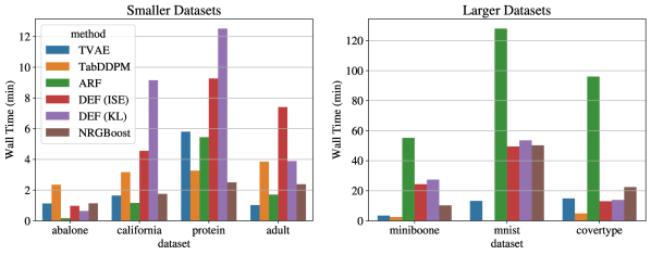
In Figure 4 we show the training times for NRGBoost as well as the other methods for the best model selected by hyperparameter tuning. We do not report the training times for the RFDE method because it is virtually free when compared to the other methods since the splitting process is random and depends only on the input domain. The data itself is only required for computing leaf probabilities which is inexpensive.
Note that the biggest computational cost for training a NRGBoost model is the Gibbs sampling (accounting for roughly 70% of the training time on average). This could potentially be improved by leveraging higher parallelism than what we used in the experiments (16 virtual cores).
We note also that we believe there is still plenty of margin for optimizing the tree-fitting code used for DEF models. As such, the results presented are merely indicative.
The computational effort for fitting a tree-based model should scale linearly both in the number of samples and the number of features and this is the main source of variation for the training times between datasets. However, we note that larger datasets can benefit more from larger models (e.g., with a larger number of leaves) which are also slower to train.
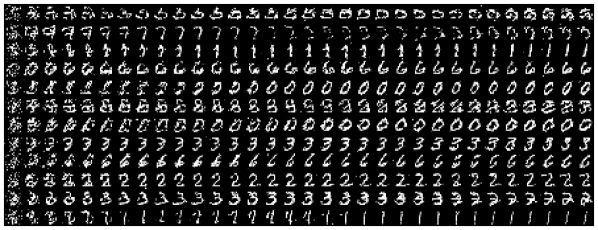
E.2 MCMC Chain Convergence on MNIST
In Figure 5 we show the convergence of a Gibbs sampler sampling from a NRGBoost model. In only a few samples each chain appears to have converged to the data manifold after starting at a random sample from the initial model (a mixture between the product of training marginals and a uniform). Note how consecutive samples are autocorrelated. In particular it can be rare for a chain to switch between two different modes of the distribution (e.g., switching digits) even though a few such transitions can be observed.