PRF: Parallel Resonate and Fire Neuron for Long Sequence Learning in Spiking Neural Networks
Abstract
Recently, there is growing demand for effective and efficient long sequence modeling, with State Space Models (SSMs) proving to be effective for long sequence tasks. To further reduce energy consumption, SSMs can be adapted to Spiking Neural Networks (SNNs) using spiking functions. However, current spiking-formalized SSMs approaches still rely on float-point matrix-vector multiplication during inference, undermining SNNs’ energy advantage. In this work, we address the efficiency and performance challenges of long sequence learning in SNNs simultaneously. First, we propose a decoupled reset method for parallel spiking neuron training, reducing the typical Leaky Integrate-and-Fire (LIF) model’s training time from to , effectively speeding up the training by to on sequence lengths to . To our best knowledge, this is the first time that parallel computation with a reset mechanism is implemented achieving equivalence to its sequential counterpart. Secondly, to capture long-range dependencies, we propose a Parallel Resonate and Fire (PRF) neuron, which leverages an oscillating membrane potential driven by a resonate mechanism from a differentiable reset function in the complex domain. The PRF enables efficient long sequence learning while maintaining parallel training. Finally, we demonstrate that the proposed spike-driven architecture using PRF achieves performance comparable to Structured SSMs (S4), with two orders of magnitude reduction in energy consumption, outperforming Transformer on Long Range Arena tasks. 111The GitHub repository will be released after paper accepted.
1 Introduction
Long Sequence Modeling. Long sequence modeling is a fundamental problem in machine learning. This significant advancement has yielded wide-ranging impact across various fields (such as Transformer Vaswani et al. (2017) and Mamba Gu & Dao (2023)), including reinforcement learning (e.g., robotics and autonomous driving) Chen et al. (2021), autoregressive task (e.g., large language models) Zhao et al. (2023), generative tasks (e.g., diffusion model) Peebles & Xie (2023) and etc. The Transformer architecture Vaswani et al. (2017), which combines token mixing with self-attention and channel mixing with dense matrices, has been successfully applied in these fields, since sequence data (with length ) is well modeled by the self-attention mechanism.
State space models (SSMs) Gu et al. (2022a) effectively address the limitations of self-attention machanism in processing long sequences by reducing computational complexity from to during inference Feng et al. (2024). The recurrent form of SSMs allows themselves to scale to longer sequence lengths more efficiently. Furthermore, the (Structured) SSMs utilize orthogonal polynomial bases to initialize recurrent weights Gu et al. (2020) for token mixing, and to compress input history Gu et al. (2021) into hidden state that enables long sequence learning yielding superior performance than Transformer models on long sequence tasks Gu et al. (2022a). As a result, variants of SSMs (e.g. Mamba Gu & Dao (2023)) are successfully applied across various fields. However, SSMs still requires large number of float-point matrix-vector multiplications for both token mixing and channel mixing to effectively extract information. These dense matrix multiplication computations scale quadratically with model size , consuming significant amount of energy during inference.
Spiking Neural Networks. SNNs benefit from the ability to convert the Float-Point (FP) Multiply Accumulate (MAC) computations into sparse Accumulate (AC) computations through their spike-driven mechanism Hu et al. (2021); Yao et al. (2024). Prior arts incorporated the spiking function at the input of token and channel mixing in SSMs to reduce energy consumption in channel mixing Stan & Rhodes (2023); Bal & Sengupta (2024); Shen et al. (2024). However, the token mixing operation within the SSMs blocks has yet been optimized, resulting in extensive FP matrix-vector multiplications and thus compromising the overall energy efficiency Stan & Rhodes (2023). To avoid FP matrix-vector multiplication computations in both channel mixing and token mixing, it is also crucial to reduce the complexity of token mixing. Therefore, we must revisit and design novel the spiking neurons in SNNs to enabl effective long sequence learning capabilities, while maintaining computation efficiency.
The Challenges for SNNs. There are two challenges in implementing long sequence learning in SNNs. (i) First, the Backpropagation Through Time (BPTT) is the commonly used training method for SNNs Wu et al. (2018). However, BPTT leads to a quadratic growth in training time with respect to sequence length, scaling as Kag & Saligrama (2021). While there are some existing SNN efficient training methods that can improve training efficiency Bellec et al. (2020); Xiao et al. (2022); Yin et al. (2023), they are still outperformed by BPTT for longer sequences Meng et al. (2023). (ii) Secondly, commonly used spiking neuron models struggle to capture long-range dependencies. Specifically, the widely used LIF neuron has difficulty in capturing and distinguishing dependencies in membrane potential over long intervals, which limits its performance on long-range tasks.Previous work attempted to address the training efficiency and performance improvement separately by improving neuron models Fang et al. (2024); Spieler et al. (2024). Fang et al. (2024); Spieler et al. (2024). However, efforts made to tackle these challenges on long sequence tasks at the same time remains unveiled. In this work, we aim for addressing these two challenges simultaneously. Our contributions are summarized as follows:
-
•
To accelerate the training process, we propose a novel decoupled reset method to implement parallel training that is equivalent to sequential training. This approach accelerates the back propagation by three orders of magnitude and can be applied to any types of spiking neurons.
-
•
To effectively extract long range dependencies, we propose the Parallel Resonate and Fire (PRF) neuron with oscillating membrane potential in complex domain leveraging an adaptive and differentiable reset mechanism.
-
•
To minimize inference energy, we further incorporate PRF into the design of Spike Driven Temporal and Channel Mixer (SD-TCM) module. This module achieves performance comparable to S4 in long range arena tasks while reducing the inference energy by two orders of magnitude.
2 Related Work
State Space Models
A general discrete form of SSMs is given by the equation: , , where , , matrices is shape with the model size and hidden size . The success of the Structured SSMs (S4) arises from the fact that the coefficients of the orthogonal bases are solved to fit an arbitrary sequence curve Gu et al. (2020). By leveraging orthogonal polynomial bases for initializing structured matrices and , S4 effectively compresses input history and outperforms transformers in long-range sequence tasks Gu et al. (2021). Subsequent variants of SSMs have also achieved great success on long sequence task Gu et al. (2022a); Goel et al. (2022b); Gu et al. (2023; 2022b); Orvieto et al. (2023). However, these SSMs-based model still exist power consumption issues that scale quadratically with model size . This is largely due to the use of the dense matrices for channel mixing after , such as in the GLU block Dauphin et al. (2017), which requires computation in matrices, leading to a significant number of FP-MAC operations.
Spikinglized SSMs
The spike mechanism can alleviate the energy problem in dense matrices by converting the FP-MAC as sparse FP-AC computation. Some spiking-formalized (spikinglized) approaches integrate the spike function into SSMs after token mixing to reduce the FP-MAC computation of channel mixing. For instance, Oliver et al.Stan & Rhodes (2023) make intersection of SNNs with S4D model Gu et al. (2022b) for long-range sequence modelling, by adding Heaviside function to token mixing output, , at each SSMs layer. Similarly, Abhronil et al.Bal & Sengupta (2024) combine stochastic spiking function at the output of . These spikinglized method can harvest the long sequence learning capability of SSMs models, but also retain nonlinear activation computation and FP matrix-vector multiplications, as they retain the , and matrices during recurrent inference. However, this retention limits the energy efficiency advantages of SNNs and poses challenges for deploying the model on neuromorphic chips. Therefore, we aim to further optimize the inference process by reducing matrices and to vectors and eliminating . This requires rethinking the role of spiking neurons in long sequence learning.
3 Problem Formulation
In this section, we first introduce the commonly used Leaky Integrate-and-Fire (LIF) neuron, then we describe the two main challenge for long range learning ability with spiking neuron.
3.1 The Leaky Integrate-and-Fire (LIF) Neuron
The LIF model is a widely used spiking neuron model. It simulates neurons by integrating input signals and firing spikes when the membrane potential exceeds a threshold. The dynamic of membrane potential is followed by:
| (1) |
where the is the input current. The constants , , and denote the membrane time constant, reset potential, and resistance. We use as in previous work. When reaches the threshold , the neuron fires a spike, and then resets to . The discrete LIF model is expressed as:
| (2) | ||||
| (3) |
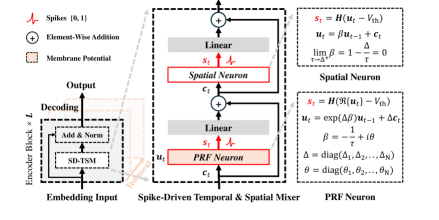
where , and the discrete timesteps , the initial situation . After firing, the membrane potential resets according to previous spike . This spiking neuron face two primary challenges for long sequence tasks: (i) The coupled reset prevents parallel training along timesteps, causing training time significantly for long sequences. (ii) The commonly used LIF neuron model struggles to capture long-range dependencies, hindering the performance on long sequence tasks. The overview as shown in Figure 1.
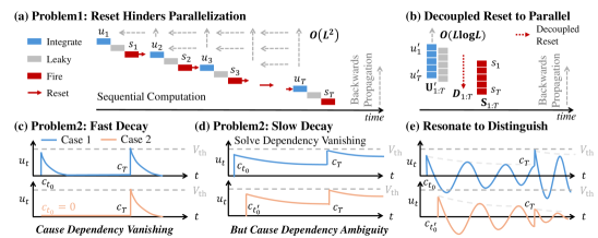
3.2 Problem 1: Coupled Reset Prevents Parallelism along Timesteps
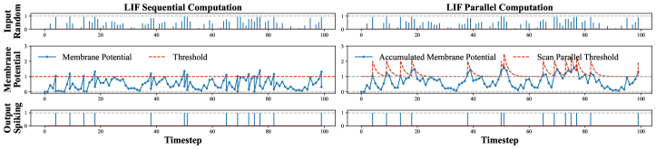
The first problem is that the training cost of LIF-based sequential computation increases exponentially as the number of timesteps extends, with a complexity of . This occurs because BPTT method requires the computational graph to expand along the time dimension Kag & Saligrama (2021). While the sequential computation of linear combination can be parallelized to reduce the time cost complexity from to during training, as done in SSMs. However, the dependency on previous spikes output with nonlinear Heaviside function. By recursively expanding and simplifying in Equation 4:
| (4) |
The reset mechanism causes to depend on all previous spike outputs. This coupling hinders the neuron’s ability to perform parallel computations, further limiting effective parallel computation for both and , as illustrated in Figure 1 (a). This forces the spiking neuron to compute sequentially. Consequently, as the number of timesteps increases during training, the time cost grows quadratically. To address this issue, we propose the decoupled reset method, which facilitates parallel computation of spiking neurons with the reset mechanism (Illustrated in Figure 1(b) and discussed in Method 4.1).
3.3 Problem 2: Commonly Used LIF Struggle with Long-Range Dependencies
The second problem is that the commonly used LIF model struggles to capture and distinguish the dependencies in the membrane potential over long interval. This limitation arises due to the dilemma of decay factor in the membrane potential dynamics. When is small, the membrane potential decreases rapidly. This Fast Decay cause the neuron to quickly forget past inputs (Figure 1 (c)). For example, in Case , if there are two inputs, and , separated by time steps, result in becoming independent of . Similarly, in Case , with zero input , the result is identical with Case . This failure to retain long-term information leads to the vanishing of dependencies. Conversely, when is large, the membrane potential retains its value over an extended period (Figure 1 (d)). This Slow Decay can solve the dependency vanishing problem, but causing ambiguity between closely spaced inputs. For instance, input with result in similar membrane potentials, there is small difference between the membrane potential in Case and the in Case , as shown in Figure 1 (d). To address this challenge, we propose enhancing the neuron’s dynamics by incorporating resonate mechanism. This allows neurons to remain sensitive to input, even after a long interval of . (Illustrated in Figure 1 (e) and discussed in detail in Method 4.2).
4 Method
In this section, we present our approach to address two primary challenges in SNNs: parallel training and long-range dependency learning. For parallel training, we decouple the reset mechanism from the integrate computation to implement parallel training while maintaining equivalence with sequential computation. For long-range dependency learning, we propose the Parallel Resonate and Fire (PRF) Neuron by incorporating the reset process as an imaginary part into the time constant, enabling the neuron to achieve long-range learning ability.
4.1 decoupled reset for Parallel Computation
To enable parallel computation, we need to decouple the causal relationship with previous spikes, by separating the linear combination part from the nonlinear causal dependency part. To achieve this, we first substitute the Equation 4 into the Equation 3 by expanding the in the Heaviside function. Then we merge the reset part into the threshold . As such, Equation 3 is rewritten as Equation 5:
| (5) |
where the linear combination of leaky and integrate part is defined as , the second part is defined as the decoupled reset . Now the spike output is:
| (6) |
where this spike output depends on and . Note that the first part is linear combination of , we define the sequence of as the ordered set over all timesteps (detailed notation is described in Appendix A). This linear combination of can be computed using convolution and further accelerated by converting the convolution into multiplication after applying the Fast Fourier Transform: , with the computation complexity, avoiding the training time in BPTT.
After efficient parallel computation of , the still remains the dependency relationship with previous spikes . To further decouple this dependency from the spike output , the key idea is converting the recursive form to the iterative form. We first define the dependency part as , as shown in Equation 7. Now, we only need to convert the from its recursive form into an iterative form. By separating the last spike from all previous spikes, we obtain Equation 8. The left part of this equation corresponds to Equation 6, while the right part refers to the recursive dependency itself, leading to Equation 9 and Equation 10:
| (7) | ||||
| (8) | ||||
| (9) | ||||
| (10) |
where the sequence of is calculated according to the sequence of , by dynamically updating :
| (11) |
At this point, all recursive forms have been converted into dynamic equations. The formation of is completely independent of . The decoupled reset function is deduced as shown in Equation 10 and 11, where can be dynamically scanned from all with complexity.
In summary, we convert the all calculation of with complexity into a combination of with complexity and subsequently with complexity, achieving a training speed-up of approximately . To summarize, this approach facilitates parallel computation: (12a) (12b) (12c) (12d) (13a) (13b) (13c) (13d)
Where the outputs from Equation 12d is equivalent with the sequential generated from Equation 3. The kernel vector with .By combining the above equations, we obtain the parallel computation process, as shown in Algorithm.1 and 2 in Appendix.B.Although parallelized LIF solves the training problem for long sequences (Experiment 5.1), it still does not perform well on long sequences (Experiment 5.2), due to the common issue of long-range dependencies in LIF models (Problem 3.3).
4.2 Resonate for Long-Range Learning Ability
To address the challenge of capturing long-range dependencies in spiking neural networks, we introduce the Parallel Resonate-and-Fire (PRF) neuron. This neuron model extends the standard LIF neuron by incorporating a resonance mechanism into its dynamics, enabling it to retain information over longer periods while maintaining computational efficiency.
Firstly, recall the commonly used LIF model from Equation 1, the dynamics are given by: , where . To introduce more dynamic behavior, we use and to replace and in the reset part, in respectively. Then the dynamic are rewritren as:
| (14) |
To introduce membrane potential oscillations, we define a complex decay constant , where . In the vanilla LIF model, the reset is a non-continuous conditional function with in Equation 14, and the reset result is instantaneous process:
| (15) |
While this reset has proven effective, it poses challenges for efficient computation. We introduce a reset function that is both effective and computationally simple for both forward and backward propagation. We define the reset function to satisfy the condition: . Substituting this definition into Equation 14, we obtain the PRF model:
| (16) |
where the real part corresponds to the membrane potential dynamics. This formulation incorporates the reset mechanism into the time constant via the imaginary component , introducing resonance into the neuron’s behavior. When , the model reduces to the standard LIF neuron without reset. If we extend the Equation 16, we can be expressed in matrix form:
| (17) |
which give us the insight that this reset process is continuous function:
| (18) |
where this formulation treats the reset as a continuous function controlled by , allowing for a more gradual and reset process.
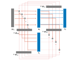
We then discretize the model (Equation 16) (details are provided in Appendix C), yielding the sequential and parallel formulations of the PRF neuron, as shown in Equation 19 and 20 in respectively:
| (19a) | ||||
| (19b) | ||||
| (19c) | ||||
| (20a) | ||||
| (20b) | ||||
Now the membrane potential ,where is the time step size. The details of parallel computation is described in Algorithm.3. Where is the input current sequence, and the kernel is calculated by:
| (21) |
with . By incorporating the imaginary component , the neuron exhibits oscillatory behavior, allowing it to resonate at specific input frequencies (see Appendix D for details). This oscillation phenomenon can be found in biological neurons Izhikevich (2001). Our model differs from variants of resonant models, like BHRF Higuchi et al. (2024), which combine adaptive thresholds and refractory mechanisms. Instead, we incorporate the reset directly into the time constant through the imaginary component while enabling efficient parallel computation for training. Furthermore, the PRF neuron can also be deployed on neuromorphic chips for inference after parallel training, requiring only two additional multiplications and one more addition than LIF (see details in Appendix E).
4.3 Theory Analysis
(1) Sequential Perspective on Dynamic. Decoupling the reset can be viewed as transforming the reduction in membrane potential caused by increased threshold value. This means that the soft reset mechanism could be equivalent to the adaptive threshold mechanism Bellec et al. (2020) as deduced in the Theorem 1. Furthermore, the LIF model without a reset can be considered a specific instance of a PRF, as demonstrated in Theorem 2. Moreover, the in PRF will converge as shown in Theorem 3. This indicates that the membrane potential of PRF is stable and bounded.
Theorem 1.
Let and in Adaptive-LIF model, then the LIF neuron with soft reset model is equivalent to the Adaptive-LIF without reset mechanism. (The proof See Appendix.F.1)
Theorem 2.
Let and , then the PRF model could degenerate as Valina LIF model without reset mechanism. (The proof see Appendix.F.2)
Theorem 3.
If the inputs follow a normal distribution, then the membrane potential of PRF will converge as a distribution , as . (The proof see Appendix.F.3)
(2) Parallel Perspective on Gradients. The issue of membrane potential dependence described in Problem 3.3 is fundamentally a problem of gradients, which are correlated with the kernel and previous spikes. Assuming the input current is across all , the gradients are proportional to:
| (22) |
here denotes the inner product, is the sequence of spike outputs from the previous layer , and represents the parallelism kernel. The subscript () indicates the sequence reversal. A small causes gradient vanishing due to a narrow receptive field, making it likely for sparse spikes to fall outside this field and yield an inner product close to zero. Conversely, a large results in a long-range, slow-decaying kernel, leading to overly consistent gradient values across spike positions. However, an oscillating kernel with a large can adjust the gradient at different spike positions, smoothing the gradients and improving the neuron’s representational capability (see Appendix G for details). Experiment 5.2 verifies this insight.
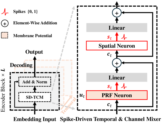
4.4 Architecture
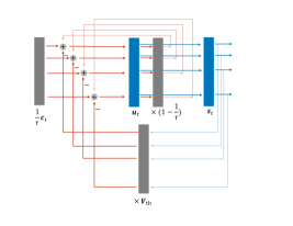
The Spike-Driven Token and Channel Mixer (SD-TCM) Module (Figure 2, with further details in Appendix H) is inspired by token and channel mixing in Transformer and S4 architectures. For token mixing, we use a PRN Neuron followed by a Linear layer, while for channel mixing, the Neuron is replaced by a Spatial Neuron. The Spatial Neuron, a variant of the LIF Neuron, focuses on instantaneous information at each timestep by setting the time constant close to 1: . This simplifies the output to , resembling motor neurons in biology with rapid decay.
During training, a trainable amplitude acts as a gate, and during inference, can be merged into the Linear layer: . Membrane shortcut residual connections are used to maintain event-driven, spike-based communication. As shown in Table 1, the PRF requires only computational complexity, while SSMs and Spikinglized SSMs require . This makes the architecture rely only on FP-AC and element-wise multiplication, reducing energy consumption and simplifying deployment on neuromorphic chips. As a result, it achieves lower computational complexity and energy consumption (see analysis in Appendix I).
| Dynamic Equation | Infer. Complexity | |
| SSMs | ||
| Spikinglized SSMs | ||
| PRF |
5 Experiments
To evaluate the efficiency and effectiveness of the parallel method, as well as the performance improvement on long sequence tasks, we first demonstrate that parallel significantly accelerates training while maintaining equivalence with sequential computation. Next, we explore the PRF neuron’s ability to handle long-range dependencies, showing that kernel oscillations improve both performance and gradient stability. Finally, the SD-TCM module achieves performance comparable to S4 while reducing energy consumption by over 98.57% on Long Range Arena tasks. Detailed experimental setups and training hyperparameters are provided in Appendix J.
5.1 The Parallel Process
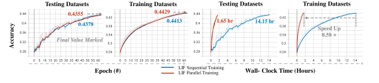
First, we compare the training runtime across different timesteps in Figure LABEL:fig.seq.par.train.time (left) using three repeated experiments. Beyond 4 timesteps, parallel training consistently outperforms sequential training. For example, at 1,024 timesteps, sequential training takes 4.6 seconds per iteration, while parallel training takes only 0.7 seconds, achieving a speedup of . This acceleration becomes more significant as the number of timesteps increases, with a speedup of at 16,384 timesteps and at 32,768 timesteps. The equivalence between sequential and parallel computation is maintained during inference and training, with only a minor accuracy difference during training (details in Appendix K), which we tentatively attribute to numerical error.
The speedup is primarily due to parallel training avoiding the recursive unfolding of the computational graph. The forward and backward passes are accelerated by and , respectively, as shown in Figure LABEL:fig.seq.par.train.time (right). The significant speedup in the backward pass occurs because sequential training requires unfolding the graph at each timestep, which is time-consuming, whereas parallel training computes the graph only once. Further details of the timing for both training and inference can be found in Appendix L.
5.2 The Long Range Learning Ability
Although parallelized LIF can speed up training, it still struggles with performance on simple long-sequence tasks, such as sequential-MNIST, as shown in Figure LABEL:fig.long.range.dependency.perspective (left). However, after introducing oscillations in the kernel, the PRF neuron successfully solves the sequential-MNIST problem, achieving both training efficiency and effectiveness.
To better understand how oscillating membrane potential improves performance, we compare the performance of various values, with and without oscillations, on the more challenging permuted-sMNIST dataset. The results after training for 50 epochs are summarized in Figure LABEL:fig.long.range.dependency.perspective (right). (We fit and set while varying the hyperparameter without training.) Without the oscillating term, as increases, accuracy initially improves as expected but then decreases beyond a certain point. In contrast, the introduction of oscillations helps counteract this decline and further enhances performance, indicating that oscillations can improve performance for long sequences.
We further examine the loss landscape contours Li et al. (2018) for each case in Figure LABEL:fig.loss.landscape, corresponding to Figure LABEL:fig.long.range.dependency.perspective (right). Gradients are perpendicular to the contour lines, with sparse or dense contours indicating smaller or larger gradients, respectively. Extremely sparse or dense contours suggest vanishing or exploding gradients. In Figure LABEL:fig.loss.landscape (a), fast decay with a small shows gradient vanishing, with extremely sparse contours. Increasing with moderate decay can alleviate gradient vanishing, but the model still encounters a local optima region (Figure LABEL:fig.loss.landscape (b)). Further increasing with slow decay is expected to fully address the vanishing problem but introduces gradient ambiguity with overlapping contours (Figure LABEL:fig.loss.landscape (c)). In contrast, the introduced oscillation from resonate results in smoother gradients (Figure LABEL:fig.loss.landscape (d)), enabling more effective feature extraction.
As shown in Table 2, the PRF neuron uses only parameters ( for neurons and for synapses) to achieve state-of-the-art (SOTA) results while maintaining training efficiency. Previous models required recurrent connections in the linear layers to solve the (p)s-MNIST task. To align the training parameters, we modified the architecture to a feedforward linear layer with a 1-(128)3-10 structure. Using parallel computation, we completed the entire training process in only hours with a batch size of 256 for 200 epochs.
|
Spiking Neuron |
|
|
|
|
||||||||||
| sMNIST (784) | LIF | ✓ | ✗ | 85.1 / 155.1* | 72.06 / 89.28 | ||||||||||
| PLIF Fang et al. (2021) | ✓ | ✗ | 85.1 / 155.1* | 87.92 / 91.79 | |||||||||||
| GLIF Yao et al. (2022) | ✓ | ✗ | 87.5 / 157.5* | 95.27 / 96.64 | |||||||||||
| TC-LIF Zhang et al. (2024) | ✓ | ✗ | 85.1 / 155.1* | 97.35 / 99.20 | |||||||||||
| ALIF Yin et al. (2021) | ✓ | ✗ | 156.3* | 98.70 | |||||||||||
| AHP Rao et al. (2022) | ✓ | ✗ | 68.4* | 96.00 | |||||||||||
| BHRF Higuchi et al. (2024) | ✓ | ✗ | 68.9 | 99.1 ± 0.1 | |||||||||||
| PRF (Ours) | ✓ | ✓ | 68.9 | 99.18 | |||||||||||
| psMNIST (784) | LIF | ✓ | ✗ | 155.1* | 80.36 | ||||||||||
| GLIF Yao et al. (2022) | ✓ | ✗ | 157.5* | 90.47 | |||||||||||
| TC-LIF Zhang et al. (2024) | ✓ | ✗ | 155.1* | 95.36 | |||||||||||
| ALIF Yin et al. (2020; 2021) | ✓ | ✗ | 156.3* | 94.30 | |||||||||||
| BHRF Higuchi et al. (2024) | ✓ | ✗ | 68.9 | 95.2 | |||||||||||
| PRF (Ours) | ✓ | ✓ | 68.9 | 96.87 |
5.3 Long Range Arena Tasks
To demonstrate the long-range dependency analysis capability of our SD-TCM module, we evaluate it using the Long Range Arena (LRA) benchmark Tay et al. (2020). This benchmark covers a wide range of classification tasks, including both textual and image domains. For the ListOps, Text, and Retrieval tasks, we use the causal architecture, while S4 employs a bidirectional architecture for all tasks. For the Image and Pathfinder tasks, we use a bidirectional architecture.
| Metric | Model | ListOps | Text | Retrieval | Image | Pathfinder | Avg. |
| En.(mJ) | S4 Ours | 5.104 0.075 | 3.718 0.298 | 24.439 0.211 | 19.222 0.187 | 6.256 0.067 | 11.748 0.168 |
| Acc.(%) | S4 Ours | 59.60 59.20 | 86.82 86.33 | 90.90 89.88 | 88.65 84.77 | 94.20 91.76 | 84.03 82.39 |
| Par. | S4 Ours | 815 k 272 k | 843 k 830 k | 3.6 M 1.1 M | 3.6 M 4.1 M | 1.3 M 1.3 M | - - |
| Text (4096) | Acc. (%) | Diff. (%) |
| without | 85.75 | |
| + on & | 85.69 | 0.06 |
| + on | 86.11 | 0.36 |
| + on | 86.33 | 0.58 |
The SD-TCM module achieves performance comparable to S4 while reducing energy consumption by over 98.57% on average, as shown in Table 4. Specifically, the accuracy on ListOps is 59.60%, compared to S4’s 59.20%. The key advantage is the significant reduction in energy consumption, as shown in Table 4, with ListOps dropping from 5.104 mJ to 0.075 mJ. This energy reduction mainly benefits from the extreme sparsity of spikes, with detailed firing rate statistics provided in Appendix M. Additionally, the model is sensitive to the imaginary part of , causing fluctuations with different initialization (see Appendix N for details). Table 4 shows an ablation study on the parameter in the Text (4096) task. Applying to both the spatial () and PRF () components slightly lowers accuracy from 85.75% to 85.69%, but applying it only to improves accuracy to 86.33%, demonstrating its benefit for spatial dependencies. Finally, as shown in Table 5, our module achieves performance comparable to the S4 baseline across tasks while preserving spike-driven feature, avoiding nonlinear activation functions and FP MAC operations.
| Model | NL Act. | FP MAC | ListOps | Text | Retrieval | Image | Pathfinder | Avg. |
| (Input length) | -Free | -Free | (2,048) | (4,096) | (4,000) | (1,024) | (1,024) | |
| Random (Lower Bound) | - | - | 10.00 | 50.00 | 50.00 | 10.00 | 50.00 | 34.00 |
| Transformer Vaswani et al. (2017) | ✗ | ✗ | 36.37 | 64.27 | 57.46 | 42.44 | 71.40 | 54.39 |
| S4 (Bidirectional) Gu et al. (2022a) | ✗ | ✗ | 59.60 | 86.82 | 90.90 | 88.65 | 94.20 | 84.03 |
| Binary S4D Stan & Rhodes (2023) | ✗ | ✗ | 54.80 | 82.50 | 85.03 | 82.00 | 82.60 | 77.39 |
| GSU & GeLU | ✗ | ✗ | 59.60 | 86.50 | 90.22 | 85.00 | 91.30 | 82.52 |
| Stoch. SpikingS4 Bal & Sengupta (2024) | ✗ | ✗ | 55.70 | 77.62 | 88.48 | 80.10 | 83.41 | 77.06 |
| SpikingSSMs Shen et al. (2024) | ✗ | ✗ | 60.23 | 80.41 | 88.77 | 88.21 | 93.51 | 82.23 |
| Spiking LMU Liu et al. (2024) | ✓ | ✗ | 37.30 | 65.80 | 79.76 | 55.65 | 72.68 | 62.23 |
| ELM Neuron Spieler et al. (2024) | ✗ | ✗ | 44.55 | 75.40 | 84.93 | 49.62 | 71.15 | 69.25 |
| Spike-Driven TCM | ✓ | ✓ | 59.20 | 86.33 | 89.88 | 84.77 | 91.76 | 82.39 |
6 Conclusion
This study aims to solve the SNNs problem of parallelization and performance on long sequences. We propose the decoupled reset method, enabling spiking neurons could parallel training. This method can be applied to any type of neuron to speed up. Additionally, we introduce the PRF neuron, incorporating the reset as an imaginary part to formulate oscillations in the membrane potential, which solves the long-range dependency problem. The SD-TCM model, combined with PRF neurons, achieves performance comparable to S4 on the LRA task while reducing energy consumption by two orders of magnitude. However, due to the sensitivity of training to neuron initialization, the PathX problem remains unsolved. This issue could be solved in the future by using better hyperparameters and initialization strategies.
References
- Bal & Sengupta (2024) Malyaban Bal and Abhronil Sengupta. Rethinking spiking neural networks as state space models. arXiv preprint arXiv:2406.02923, 2024.
- Bellec et al. (2020) Guillaume Bellec, Franz Scherr, Anand Subramoney, Elias Hajek, Darjan Salaj, Robert Legenstein, and Wolfgang Maass. A solution to the learning dilemma for recurrent networks of spiking neurons. Nature communications, 11(1):3625, 2020.
- Chen et al. (2021) Lili Chen, Kevin Lu, Aravind Rajeswaran, Kimin Lee, Aditya Grover, Misha Laskin, Pieter Abbeel, Aravind Srinivas, and Igor Mordatch. Decision transformer: Reinforcement learning via sequence modeling. Advances in neural information processing systems, 34:15084–15097, 2021.
- Dauphin et al. (2017) Yann N Dauphin, Angela Fan, Michael Auli, and David Grangier. Language modeling with gated convolutional networks. In International conference on machine learning, pp. 933–941. PMLR, 2017.
- Davies et al. (2018) Mike Davies, Narayan Srinivasa, Tsung-Han Lin, Gautham Chinya, Yongqiang Cao, Sri Harsha Choday, Georgios Dimou, Prasad Joshi, Nabil Imam, Shweta Jain, et al. Loihi: A neuromorphic manycore processor with on-chip learning. Ieee Micro, 38(1):82–99, 2018.
- Fang et al. (2021) Wei Fang, Zhaofei Yu, Yanqi Chen, Timothée Masquelier, Tiejun Huang, and Yonghong Tian. Incorporating learnable membrane time constant to enhance learning of spiking neural networks. In Proceedings of the IEEE/CVF international conference on computer vision, pp. 2661–2671, 2021.
- Fang et al. (2024) Wei Fang, Zhaofei Yu, Zhaokun Zhou, Ding Chen, Yanqi Chen, Zhengyu Ma, Timothée Masquelier, and Yonghong Tian. Parallel spiking neurons with high efficiency and ability to learn long-term dependencies. Advances in Neural Information Processing Systems, 36, 2024.
- Feng et al. (2024) Leo Feng, Frederick Tung, Hossein Hajimirsadeghi, Mohamed Osama Ahmed, Yoshua Bengio, and Greg Mori. Attention as an rnn. arXiv preprint arXiv:2405.13956, 2024.
- Goel et al. (2022a) Karan Goel, Albert Gu, Chris Donahue, and Christopher Ré. It’s raw! audio generation with state-space models. In International Conference on Machine Learning, pp. 7616–7633. PMLR, 2022a.
- Goel et al. (2022b) Karan Goel, Albert Gu, Chris Donahue, and Christopher Ré. It’s raw! audio generation with state-space models. International Conference on Machine Learning (ICML), 2022b.
- Gu & Dao (2023) Albert Gu and Tri Dao. Mamba: Linear-time sequence modeling with selective state spaces. arXiv preprint arXiv:2312.00752, 2023.
- Gu et al. (2020) Albert Gu, Tri Dao, Stefano Ermon, Atri Rudra, and Christopher Ré. Hippo: Recurrent memory with optimal polynomial projections. Advances in neural information processing systems, 33:1474–1487, 2020.
- Gu et al. (2021) Albert Gu, Isys Johnson, Karan Goel, Khaled Saab, Tri Dao, Atri Rudra, and Christopher Ré. Combining recurrent, convolutional, and continuous-time models with linear state-space layers. Advances in Neural Information Processing Systems, 34, 2021.
- Gu et al. (2022a) Albert Gu, Karan Goel, and Christopher Ré. Efficiently modeling long sequences with structured state spaces. In The International Conference on Learning Representations (ICLR), 2022a.
- Gu et al. (2022b) Albert Gu, Ankit Gupta, Karan Goel, and Christopher Ré. On the parameterization and initialization of diagonal state space models. Advances in Neural Information Processing Systems, 35, 2022b.
- Gu et al. (2023) Albert Gu, Isys Johnson, Aman Timalsina, Atri Rudra, and Christopher Ré. How to train your hippo: State space models with generalized basis projections. In The International Conference on Learning Representations (ICLR), 2023.
- Higuchi et al. (2024) Saya Higuchi, Sebastian Kairat, Sander M Bohte Otte, et al. Balanced resonate-and-fire neurons. arXiv preprint arXiv:2402.14603, 2024.
- Hu et al. (2021) Yangfan Hu, Huajin Tang, and Gang Pan. Spiking deep residual networks. IEEE Transactions on Neural Networks and Learning Systems, 34(8):5200–5205, 2021.
- Hu et al. (2024) Yifan Hu, Lei Deng, Yujie Wu, Man Yao, and Guoqi Li. Advancing spiking neural networks toward deep residual learning. IEEE Transactions on Neural Networks and Learning Systems, 2024.
- Izhikevich (2001) Eugene M Izhikevich. Resonate-and-fire neurons. Neural networks, 14(6-7):883–894, 2001.
- Kag & Saligrama (2021) Anil Kag and Venkatesh Saligrama. Training recurrent neural networks via forward propagation through time. In International Conference on Machine Learning, pp. 5189–5200. PMLR, 2021.
- Krizhevsky (2009) Alex Krizhevsky. Learning multiple layers of features from tiny images. Master’s thesis, University of Toronto, 2009.
- Li et al. (2018) Hao Li, Zheng Xu, Gavin Taylor, Christoph Studer, and Tom Goldstein. Visualizing the loss landscape of neural nets. Advances in neural information processing systems, 31, 2018.
- Linsley et al. (2018) Drew Linsley, Junkyung Kim, Vijay Veerabadran, Charles Windolf, and Thomas Serre. Learning long-range spatial dependencies with horizontal gated recurrent units. Advances in Neural Information Processing Systems, 31, 2018.
- Liu et al. (2024) Zeyu Liu, Gourav Datta, Anni Li, and Peter Anthony Beerel. LMUFormer: Low complexity yet powerful spiking model with legendre memory units. In The Twelfth International Conference on Learning Representations, 2024. URL https://openreview.net/forum?id=oEF7qExD9F.
- Maas et al. (2011) Andrew Maas, Raymond Daly, Peter Pham, Dan Huang, Andrew Ng, and Christopher Potts. Learning word vectors for sentiment analysis. In Proceedings of the 49th Annual Meeting of the Association for Computational Linguistics: Human Language Technologies, pp. 142–150, 2011.
- Meng et al. (2023) Qingyan Meng, Mingqing Xiao, Shen Yan, Yisen Wang, Zhouchen Lin, and Zhi-Quan Luo. Towards memory-and time-efficient backpropagation for training spiking neural networks. In Proceedings of the IEEE/CVF International Conference on Computer Vision, pp. 6166–6176, 2023.
- Nangia & Bowman (2018) Nikita Nangia and Samuel Bowman. ListOps: A diagnostic dataset for latent tree learning. NAACL HLT 2018, pp. 92, 2018.
- Orvieto et al. (2023) Antonio Orvieto, Samuel L Smith, Albert Gu, Anushan Fernando, Caglar Gulcehre, Razvan Pascanu, and Soham De. Resurrecting recurrent neural networks for long sequences. In International Conference on Machine Learning, pp. 26670–26698. PMLR, 2023.
- Paszke et al. (2019) Adam Paszke, Sam Gross, Francisco Massa, Adam Lerer, James Bradbury, Gregory Chanan, Trevor Killeen, Zeming Lin, Natalia Gimelshein, Luca Antiga, et al. Pytorch: An imperative style, high-performance deep learning library. Advances in neural information processing systems, 32, 2019.
- Peebles & Xie (2023) William Peebles and Saining Xie. Scalable diffusion models with transformers. In Proceedings of the IEEE/CVF International Conference on Computer Vision, pp. 4195–4205, 2023.
- Radev et al. (2009) Dragomir Radev, Pradeep Muthukrishnan, and Vahed Qazvinian. The ACL anthology network corpus. ACL-IJCNLP 2009, pp. 54, 2009.
- Rao et al. (2022) Arjun Rao, Philipp Plank, Andreas Wild, and Wolfgang Maass. A long short-term memory for ai applications in spike-based neuromorphic hardware. Nature Machine Intelligence, 4(5):467–479, 2022.
- Shen et al. (2024) Shuaijie Shen, Chao Wang, Renzhuo Huang, Yan Zhong, Qinghai Guo, Zhichao Lu, Jianguo Zhang, and Luziwei Leng. Spikingssms: Learning long sequences with sparse and parallel spiking state space models. arXiv preprint arXiv:2408.14909, 2024.
- Smith et al. (2023) Jimmy T.H. Smith, Andrew Warrington, and Scott Linderman. Simplified state space layers for sequence modeling. In The Eleventh International Conference on Learning Representations, 2023. URL https://openreview.net/forum?id=Ai8Hw3AXqks.
- Spieler et al. (2024) Aaron Spieler, Nasim Rahaman, Georg Martius, Bernhard Schölkopf, and Anna Levina. The expressive leaky memory neuron: an efficient and expressive phenomenological neuron model can solve long-horizon tasks. In The Twelfth International Conference on Learning Representations, 2024. URL https://openreview.net/forum?id=vE1e1mLJ0U.
- Stan & Rhodes (2023) Matei Ioan Stan and Oliver Rhodes. Learning long sequences in spiking neural networks. arXiv preprint arXiv:2401.00955, 2023.
- Tay et al. (2020) Yi Tay, Mostafa Dehghani, Samira Abnar, Yikang Shen, Dara Bahri, Philip Pham, Jinfeng Rao, Liu Yang, Sebastian Ruder, and Donald Metzler. Long range arena: A benchmark for efficient transformers. arXiv preprint arXiv:2011.04006, 2020.
- Tay et al. (2021) Yi Tay, Mostafa Dehghani, Samira Abnar, Yikang Shen, Dara Bahri, Philip Pham, Jinfeng Rao, Liu Yang, Sebastian Ruder, and Donald Metzler. Long Range Arena: A benchmark for efficient transformers. In International Conference on Learning Representations, 2021.
- Vaswani et al. (2017) Ashish Vaswani, Noam Shazeer, Niki Parmar, Jakob Uszkoreit, Llion Jones, Aidan N Gomez, Łukasz Kaiser, and Illia Polosukhin. Attention is all you need. Advances in neural information processing systems, 30, 2017.
- Wu et al. (2018) Yujie Wu, Lei Deng, Guoqi Li, Jun Zhu, and Luping Shi. Spatio-temporal backpropagation for training high-performance spiking neural networks. Frontiers in neuroscience, 12:331, 2018.
- Xiao et al. (2022) Mingqing Xiao, Qingyan Meng, Zongpeng Zhang, Di He, and Zhouchen Lin. Online training through time for spiking neural networks. Advances in neural information processing systems, 35:20717–20730, 2022.
- Yao et al. (2024) Man Yao, Jiakui Hu, Zhaokun Zhou, Li Yuan, Yonghong Tian, Bo Xu, and Guoqi Li. Spike-driven transformer. Advances in Neural Information Processing Systems, 36, 2024.
- Yao et al. (2022) Xingting Yao, Fanrong Li, Zitao Mo, and Jian Cheng. Glif: A unified gated leaky integrate-and-fire neuron for spiking neural networks. Advances in Neural Information Processing Systems, 35:32160–32171, 2022.
- Yin et al. (2020) Bojian Yin, Federico Corradi, and Sander M Bohté. Effective and efficient computation with multiple-timescale spiking recurrent neural networks. In International Conference on Neuromorphic Systems 2020, pp. 1–8, 2020.
- Yin et al. (2021) Bojian Yin, Federico Corradi, and Sander M Bohté. Accurate and efficient time-domain classification with adaptive spiking recurrent neural networks. Nature Machine Intelligence, 3(10):905–913, 2021.
- Yin et al. (2023) Bojian Yin, Federico Corradi, and Sander M Bohté. Accurate online training of dynamical spiking neural networks through forward propagation through time. Nature Machine Intelligence, 5(5):518–527, 2023.
- Zhang et al. (2024) Shimin Zhang, Qu Yang, Chenxiang Ma, Jibin Wu, Haizhou Li, and Kay Chen Tan. Tc-lif: A two-compartment spiking neuron model for long-term sequential modelling. In Proceedings of the AAAI Conference on Artificial Intelligence, volume 38, pp. 16838–16847, 2024.
- Zhao et al. (2023) Wayne Xin Zhao, Kun Zhou, Junyi Li, Tianyi Tang, Xiaolei Wang, Yupeng Hou, Yingqian Min, Beichen Zhang, Junjie Zhang, Zican Dong, et al. A survey of large language models. arXiv preprint arXiv:2303.18223, 2023.
Appendix A Notation in the Paper
Throughout this paper and in this Appendix, we use the following notations. Matrices are represented by bold italic capital letters, such as , while sequences are represented by bold non-italic capital letters, such as . For a function , we use instead of to denote the first-order derivative of with respect to . The symbols and represent the element-wise product and the inner product, respectively.
Appendix B The Algorithm of Pseudo-Code
Algorithms 1 and 2 describe the parallel computation of the LIF model, while Algorithm 3 outlines the computation process for the PRF model.
Appendix C The Discretization of PRF Neurons
Firs, we recall the PRF model:
| (23) |
where complex membrane potential and a complex decay constant with .
Note that here is treated as a fixed external current input, which is constant from the point of view of this ODE in . Let denote the average value in each discrete time interval. Assumes the value of a sample of u is held constant for a duration of one sample interval .
| (24) |
Since we only observe the real part of the membrane potential, the input is a real number. Thus, we can consider the real part to describe the model. The model can then be expressed as:
| (25) | ||||
Rearranging, assuming without input decay, we replace with , as done in S4 Gu et al. (2022a). We obtain the discrete form:
| (26) |
Finally, replacing the original part gives the PRF neuron with sequential computation:
| (27) | ||||
| (28) |
Appendix D The Frequency Response for PRF neuron
This section mainly discusses the frequency response of the dynamic reset LIF neuron. Recall the membrane potential dynamic equation:
| (29) | ||||
| (30) |
This dynamic process can be regarded as a damped harmonic oscillator. The real part of the membrane potential, , represents the displacement. When the displacement exceeds a certain value, this model will issue a signal. Here, represents the timestep size, and is the input for each timestep, driven by an external force.
First, define . The model can then be expressed as:
| (31) | ||||
| (32) |
To explore the numerical effects in the experiment, we obtain the approximate ODE by using to represent :
| (33) |
using a first-order Taylor expansion approximation, we obtain:
| (34) |
We assume the driven input is an oscillation, , with a constant base amplitude and a variable angular frequency . The position of the membrane potential will oscillate in resonance as:
| (35) |
where is the amplitude as a function of the external excitation frequency. We then have:
| (36) |
Substituting Equation 36 into Equation 34 gives:
| (37) | ||||
| (38) | ||||
| (39) |
Rearranging the equation yields:
| (40) | ||||
| (41) |
Thus, we have:
| (42) | |||
| (43) |
The magnitude can be obtained by taking the modulus, which varies with and :
| (44) | ||||
| (45) |
Assuming , the value of corresponding to the maximum of the magnitude can be found:
| (46) | ||||
| (47) | ||||
| (48) |
Therefore, the resonant frequency at the point of maximum magnitude coincides with , and .
Appendix E Deployment analysis of PRF Neuron
This model can also be easily deployed on neuromorphic chips. After training, the coefficients can merge together. Recalling the PRF Neuron as described in Equation 19, we explicitly expand the real and imaginary parts as follows:
| (49) | ||||
We use the symbols and to denote the real and imaginary parts of the membrane potential , respectively:
| (50) |
where the coefficients are the merged parameters:
| (51) | ||||
Finally, the spike is output based on the real part . For simplicity, we use and to denote and , respectively. Thus, the explicit iteration of the PRF can be written as:
| (52) | ||||
| (53) | ||||
| (54) |
Intuitively, compared to the LIF model, the PRF introduces two additional multiplication operations and one extra addition operation for inference, along with an extra hidden state that needs to be saved, as shown in Figure 5. Furthermore, this neuron model, with its double hidden state, can also be easily deployed on neuromorphic chips, similar to how the AHP model Rao et al. (2022) was deployed on the Loihi chip Davies et al. (2018).
Appendix F Proof
F.1 Proof of Theorem.1
Proof.
Firstly, consider the Adaptive LIF (ALIF) model Bellec et al. (2020), where the threshold adapts according to recent firing activity. The dynamic threshold is given by Equation 55 to Equation 57:
| (55) | ||||
| (56) | ||||
| (57) |
Here, the decay factor is given by , where is the adaptation time constant, as described in ALIF Bellec et al. (2020).
Intuitively, when , we have , simplifying Equation 57 to . The variable can be further deduced as follows:
| (58) |
| (59) |
| (60) | ||||
| (61) |
F.2 Proof of Theorem.2
Proof.
Firstly, we recall the dynamic iteration of the PRF model:
| (62) | ||||
| (63) |
Next, let and , allowing the model to be rewritten as:
| (64) | ||||
| (65) |
At this point, , meaning it only contains a real part, with the decay affecting only the real component. Setting can be interpreted as removing the reset process. Furthermore, the exponential term can be approximated using the first-order Taylor expansion:
| (66) |
Finally, the dynamic equation can be rewritten as:
| (67) | ||||
| (68) |
Equation 67 and Equation 68 are equivalent to the standard LIF model without the reset process, as given in Equation 2. ∎
F.3 Proof of Theorem.3
Proof.
Firstly, we recall the dynamic iteration of the PRF model:
| (69) |
assuming is normally distributed with zero mean and variance at time-invariant, and , , and are constants. Define the complex constant :
| (70) |
Note that the magnitude of is:
| (71) |
since . In further, where the membrane potential is the real part of .
Next, we expand recursively:
| (72) | ||||
| (73) | ||||
| (74) | ||||
| (75) | ||||
| (76) |
Now, we calculate the expectation and variation of . since are independent and identically distributed with and , we can compute the expected value of :
| (77) | ||||
| (78) | ||||
| (79) |
As , it follows that:
| (80) |
Next, compute the variance of :
| (81) | ||||
| (82) | ||||
| (83) | ||||
| (84) |
Since are independent and have zero mean, we have:
| (85) | ||||
| (86) | ||||
| (87) |
Therefore, the variance of is:
| (88) |
Since as deduced in Equation 71, we have:
| (89) |
Thus,
| (90) |
This is a finite geometric series with first term equals to and common ratio :
| (91) |
Therefore,
| (92) |
As , , so the variance approaches:
| (93) |
this is a finite constant, in summary we could get the distribution after :
| (94) |
which implies that is bounded in probability. This indicates that does not diverge but instead stabilizes to a specific distribution related to the input distribution and hyperparameters. It ensures that despite the randomness introduced by the inputs , the neuron’s response remains predictable in distribution. ∎
Appendix G Parallel Perspective on Solving Long-Range Learning Problem
From the subsection of Problem Formulation 2, we gain the insight that the gradient is proportional to the inner product of the kernel and previous layer spikes.
| (95) |
To verify this insight, we define three extreme situations (Fast Decay, Slow Decay and Slow Decay with Resonate) to explore this from the parallel kernel perspective, as shown in Figure 6.

Fast Decay
Fast decay may cause the problem of long-range dependency vanishing, as shown in Figure 6(a). The kernel decays rapidly as the time step increases. In this case, early spikes (represented by ) dominate the gradient calculation, while contributions from later spikes (represented by ) are almost negligible. As a result, the gradient is mostly proportional to , leading to the vanishing of long-range dependencies. The network struggles to learn and retain information from distant time steps, causing the gradients to vanish and impairing the learning of long-term dependencies.
Slow Decay
Slow Decay may relive the vanishing problem, but may cause gradients ambiguity as shown in Figure.6(b). This situation shows the kernel decays more slowly over time, which balances the contributions from both early and late spikes (denoted as and ). However, this slow decay introduces a new problem—ambiguity. When the contributions from different parts of the sequence are similar (e.g., ), the network finds it difficult to distinguish between these cases. This ambiguity can confuse the learning process, as the network may not correctly interpret or differentiate between distinct temporal patterns.
Slow Decay with Resonate
Resonate could may relive the ambiguity problem to capture the resonate information under the long range, as shown in Figure.6(c). the kernel oscillates or resonates, effectively capturing contributions from both early and late spikes. This resonance allows the network to amplify and preserve significant information across the entire sequence, represented by and . Such behavior is advantageous for learning long-range dependencies, as it helps maintain the gradient information over time. The network can now better distinguish between different temporal patterns, leading to improved learning and retention of long-term information, which is crucial for tasks involving long sequences.
Appendix H The Architecture for Long Range Arena Task
This Section introduces the Spike-Driven Temporal and Channel Mixing (SD-TCM) Module, as shown in Figure 7. This design philosophy mainly stems from the token and channel mixing in the transformer and S4 for solving more difficult sequence tasks. Firstly, we introduce the spatial neuron by considering the other side of LIF neurons. Secondly, we present the mixer module, which combines the PRF neuron and spatial neuron. Furthermore, we compare the computation complexity and theoretical energy consumption (Detail in Appendix.I).
The design philosophy of this module stems from combining token mixing with channel mixing, a common practice in transformer and S4 modules. The transformer uses a self-attention block for token mixing and a 2-layer MLP for channel mixing Vaswani et al. (2017). The S4 employs SSMs for token mixing and GLU for channel mixing Gu et al. (2022a). Firstly, we propose the Spatial neuron utilized for channel mixing. We consider the limitation of the time constant close to the time scale, focusing on the instantaneous information for each timestep:
| (96) |
then the output of Spatial Neuron replaced as . This type of neuron can also be observed in motor neurons in biology with extreme huge decay. According to Theorem 2, we gain the insight that the LIF neuron is a subset of the PRF Neuron. The Spatial Neuron is also a subset of the LIF Neuron, aiming to focus on instantaneous spatial information without temporal information. Consequently, we derived a special case of the LIF neuron, which we term the Spatial Neuron. In further, we use the trainable amplitude for Spatial LIF Neuron with the output . Where the amplitude constant is trainable parameters with always initialize as . After training, the amplitude constant could merge to the following Linear layer during the inference. That means .
Secondly, we design the SD-TCM module consists of three main components: the Spatial Neuron , PRF Neuron , fully-connected layer . To keep the spike-driven feature, we use the membrane shortcut residual connect Hu et al. (2024) like spike-driven transformer Yao et al. (2024). Given a input sequence , the embedding the sequence of flattened spike patches with dimensional channel,
| (97) |
where denote timestep while aligning with the sequence length. Then the SD-TCM is written as:
| (98) | ||||||
| RPE | RPE | (99) | ||||
| (100) | ||||||
| (101) |
Where is the binary value set. After the layer, the following output as the input of classifier or other head for corresponding task. This block keep the spike-driven with two properties: event-driven and binary spike-based communication. The former means that no computation is triggered when the input is zero. The binary restriction in the latter indicates that there are only additions.
The original S4 layer is unidirectional or causal, which is an unnecessary constraint for the classification tasks appearing in LRA. Goel et al. (2022a) propose a bidirectional version of S4 that simply concatenates two S4 convolution kernels back-to-back Gu et al. (2022b). As same the bidirectional model implemented in S4 block. We implement the bidirectional model by replacing the Equation 99 as the following equation:
| (102) |
where Concat and Rev means the concatenate and reverse operation along the channel and timestep dimension in respectively. We simply pass the input sequence through an PRF Neuron, and also reverse it and pass it through an independent second PRF Neuron. These spiking outputs are concatenated and passed through a position wise linear layer. Keep the same with S4 and Shashimi Goel et al. (2022a), the following Linear layer () will change the input feature dimension as the double in the bidirectional model.
Appendix I The Theoretical Analysis of Power consumption
The two tables provide a detailed comparison of inference complexity and energy consumption across various models. Table 6 compares the computational complexity involved in the inference phase for different models. Table 7 evaluates the energy consumption of these models during the token mixing and channel mixing stages.
| Dynamic Equation | Variables | Parameters | Infer. Complexity | |
| SSMs | ||||
| Spikinglized SSMs | ||||
| Ours |
| Token Mixing | Channel Mixing | |||
| Comput. | Energy | Comput. | Energy | |
| S4-LegS | ||||
| Binary S4D | ||||
| GSU | ||||
| Ours | - | - | ||
Appendix J Description of Datasets and Hyperparameters
All our experiments were conducted on an NVIDIA GeForce RTX 4090 GPU with 24 GB of memory. The specific experimental setup and hyperparameters are detailed in subsection J.1, and the description of the experimental dataset is provided in subsection J.2.
J.1 Task Specific Hyperparameters
Here we specify any task-specific details, hyperparameter or architectural differences from the defaults outlined above.
J.1.1 Sequential MNIST & Permuted Sequential MNIST
For Figure.4, we used a neural network architecture with layers of size 1-64-256-256-10 ( training parameters) with 256 batch size for training 200 epochs. All experiments were conducted using the same random seeds.
J.1.2 Long Range Arena
The total hyperparameters configure is shown in Table 8.
| Task | Depth | Channels | Norm | Pre-norm | Dropout | LR | Neuron LR | B | Epochs | WD | (, ) |
| ListOps | 8 | 128 | BN | False | 0 | 0.005 | 0.001 | 50 | 40 | 0.05 | (0.001, 0.1) |
| Text | 6 | 256 | BN | True | 0 | 0.005 | 0.001 | 16 | 32 | 0.05 | (0.001, 0.1) |
| Retrieval | 6 | 256 | BN | True | 0 | 0.005 | 0.001 | 32 | 20 | 0.05 | (0.001, 0.1) |
| Image | 6 | 512 | BN | False | 0.1 | 0.005 | 0.001 | 50 | 200 | 0.05 | (0.001, 0.1) |
| Pathfinder | 6 | 256 | BN | True | 0.05 | 0.005 | 0.001 | 64 | 200 | 0.03 | (0.001, 0.1) |
J.2 Dataset Details
We provide more context and details for (p)s-MNIST and each tasks of the LRA Tay et al. (2021). Note that we follow the same data pre-processing steps as Gu et al. (2022a), which we also include here for completeness. The following describe mainly refer from Smith et al. (2023).
-
•
Sequential MNIST: (sMNIST) 10-way digit classification from a grayscale image of a handwritten digit, where the input image is flattened into a -length scalar sequence.
-
•
Permuted Sequential MNIST: (psMNIST) 10-way digit classification from a grayscale image of a handwritten digit, where the input image is flattened into a -length scalar sequence. This sequence is then permuted using a fixed order.
-
•
ListOps: A lengthened version of the dataset presented by Nangia & Bowman (2018). Given a nested set of mathematical operations (such as min and max) and integer operands in the range zero to nine, expressed in prefix notation with brackets, compute the integer result of the mathematical expression (e.g. [max 2 6 [ min 9 7 ] 0] 7). Characters are encoded as one-hot vectors, with unique values possible (opening brackets and operators are grouped into a single token). The sequences are of unequal length, and hence the end of shorter sequences is padded with a fixed indicator value, padded to a maximum length of . A reserved end-of-sequence token is appended. There are different classes, representing the integer result of the expression. There are training sequences, validation sequences, and test sequences. No normalization is applied.
-
•
Text: Based off of the iMDB sentiment dataset presented by Maas et al. (2011). Given a movie review, where characters are encoded as a sequence of integer tokens, classify whether the movie review is positive or negative. Characters are encoded as one-hot vectors, with unique values possible. Sequences are of unequal length, and are padded to a maximum length of . There are two different classes, representing positive and negative sentiment. There are training examples and test examples. No validation set is provided. No normalization is applied.
-
•
Retrieval: Based off of the ACL Anthology network corpus presented by Radev et al. (2009). Given two textual citations, where characters are encoded as a sequence of integer tokens, classify whether the two citations are equivalent. The citations must be compressed separately, before being passed into a final classifier layer. This is to evaluate how effectively the network can represent the text. The decoder head then uses the encoded representation to complete the task. Characters are encoded into a one-hot vector with unique values. Two paired sequences may be of unequal length, with a maximum sequence length of . There are two different classes, representing whether the citations are equivalent or not. There are training pairs, validation pairs, and test pairs. No normalization is applied.
-
•
Image: Uses the CIFAR-10 dataset presented by Krizhevsky (2009). Given a grayscale CIFAR-10 image as a one-dimensional raster scan, classify the image into one of ten classes. Sequences are of equal length (). There are ten different classes. There are training examples, validation examples, and test examples. RGB pixel values are converted to a grayscale intensities, which are then normalized to have zero mean and unit variance (across the entire dataset).
-
•
Pathfinder: Based off of the Pathfinder challenge introduced by Linsley et al. (2018). A grayscale image image shows a start and an end point as a small circle. There are a number of dashed lines on the image. The task is to classify whether there is a dashed line (or path) joining the start and end point. There are two different classes, indicating whether there is a valid path or not. Sequences are all of the same length (). There are training examples, validation examples, and test examples. The data is normalized to be in the range .
Appendix K The Equivalence of Sequential and Parallel
First, the parallel computation is equivalent to sequential computation during both inference and training phases. This equivalence is clearly illustrated in Figures 8 and 9. For inference equivalence, Figure 8 shows that when applying random input to an LIF neuron using both sequential and parallel computation, the spiking output remains consistent across both methods.
For training equivalence, Figure 9 shows the training and testing curves for a CIFAR classification task with 1024-length inputs using a 5-layer MLP, where each linear layer is followed by a neuron. Inference is performed with sequential computation, while training is conducted using either sequential (blue curve) or parallel (red curve) methods. After 64 training epochs, the training and testing curves align closely, indicating that the gradient computations from both sequential and parallel training are nearly identical. The parallel method achieves an speedup with a sequence length of .
Appendix L The Parallel Implementation Case Statics Details
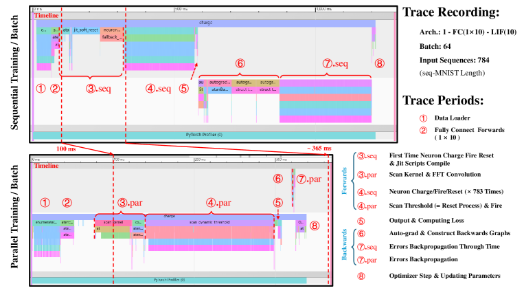
The figure presents a comparative analysis of sequential and parallel training processes using the torch.profiler tool for a sample case. The trace recording and periods timeline as shown in Figure.10. The corresponding details data statistics in the Table.10 and 10. We designed a simple case using a fully connected layer (FC: ) and an extremely simple architecture to identify the bottlenecks in sequential and parallel training. We use sequential-MNIST (784 length) with 64 batch size as the input.
| Functions | Duration () | Num. of Calls |
| Forward | ||
| Charge | 146,725 | 784 |
| Reset | 150,120 | 784 |
| Fire | 91,398 | 784 |
| Backprop (Autograd) | ||
| GraphBackward | 250,161 | 1564 |
| AtanBackward | 186,086 | 784 |
| SelectBackward | 91,438 | 784 |
| SubBackward | 20,124 | 787 |
| StackBackward | 19,436 | 1 |
| MmBackward | 1,404 | 1 |
| Other | ||
| Other | 244,358 | - |
| All | 1,201,250 | - |
| Functions | Duration () | Num. of Calls |
| Forward | ||
| Scan Kernel | 45,634 | 1 |
| FFT Conv Op. | 14,627 | 1 |
| Scan Dynamic Thr. | 158,774 | 1 |
| Fire | 459 | 1 |
| Backprop (Autograd) | ||
| FftR2CBackward | 1,099 | 1 |
| AtanBackward | 762 | 1 |
| MulBackward | 582 | 1 |
| FftC2RBackward | 235 | 1 |
| MmBackward | 1,615 | 1 |
| Other | ||
| Other | 113,863 | - |
| All | 337,650 | - |
In the sequential training timeline, each phase of forward and backward propagation happens one after the other, resulting in a total training time of approximately . These phases include data loading, fully connected forward passes, neuron charge/fire/reset operations, output computation, autograd construction, and error backpropagation. This sequential computation introduces significant delays, particularly during the repetitive neuron charging and resetting in the backward phases, which dominate the computation time.
In contrast, the parallel training timeline reduces the overall training time to around 337 ms by executing multiple forward and backward propagation phases simultaneously. This approach leverages parallel processing to handle operations such as neuron charging and threshold scanning concurrently, thereby reducing redundant delays. The comparison highlights significant efficiency gains in processes like autograd, constructing backward graphs, and error backpropagation.
Appendix M The Statistics of Fire Rate
The spiking fire rate is derived from the top-1 test accuracy model (Average in Table 11). We extract the fire rate for each layer (12 to 16). On average, the Spatial Neuron () exhibits a higher fire rate than the PRF (). The checkpoints and statistical code can be found in the open-source repository.
| Tasks | ListOps | Text | Retrieval | Image | Pathfinder |
| Avg. Fire Rate (%) | 3.53 | 4.32 | 1.48 | 3.47 | 3.29 |
| Layer | 1 | 2 | 3 | 4 | 5 | 6 | 7 | 8 |
| 0.0 | 5.17 | 2.50 | 2.83 | 0.80 | 1.17 | 3.02 | 2.22 | |
| 9.60 | 5.29 | 4.51 | 2.63 | 5.58 | 3.57 | 9.57 | 5.07 |
| Layer | 1 | 2 | 3 | 4 | 5 | 6 |
| 2.11 | 4.30 | 2.79 | 1.66 | 1.02 | 1.48 | |
| 9.20 | 9.90 | 10.11 | 7.18 | 5.55 | 5.25 |
| Layer | 1 | 2 | 3 | 4 | 5 | 6 |
| 0.66 | 0.42 | 0.42 | 0.49 | 0.48 | 0.87 | |
| 4.79 | 4.24 | 1.54 | 2.46 | 2.50 | 1.91 |
| Layer | 1 | 2 | 3 | 4 | 5 | 6 |
| 0.22 | 7.10 | 5.25 | 3.67 | 3.90 | 4.24 | |
| 0.44 | 9.90 | 5.71 | 4.35 | 2.77 | 1.07 |
| Layer | 1 | 2 | 3 | 4 | 5 | 6 |
| 3.37 | 3.96 | 5.07 | 4.53 | 4.53 | 4.78 | |
| 3.66 | 2.98 | 3.74 | 3.63 | 3.33 | 2.53 |
Appendix N The Ablation Experiments
We examine the sensitivity of the and hyper-parameters during initialization. Using a neural network architecture with layers sized 1-64-256-256-10 and a batch size of 256, we fixed and set and as non-trainable scale values. Figure LABEL:fig.init.sensitive illustrates this sensitivity for the sMNIST (left) and psMNIST (right) datasets. The gray frames highlight a shift in sensitive regions from sMNIST to psMNIST, indicating that different data distributions require careful initialization of and . Furthermore, we investigate the impact of varying initialization of values on the performance of the LRA tasks, as shown in Tables 17 - 21. The suitable initialization of is crucial.
| [0, /4] | [0, /5] | [0, /6] | [0, /7] | [0, /8] | |
| Acc. (%) | 56.85 | 55.60 | 59.20 | 58.05 | 54.55 |
| [0, ] | [0, /2] | [0, /4] | [0, /8] | [0, /16] | |
| Acc. (%) | 81.27 | 83.28 | 84.94 | 86.33 | 85.32 |
| [0, /4] | [0, /5] | [0, /6] | [0, /7] | [0, /8] | |
| Acc. (%) | 89.64 | 89.52 | 89.75 | 89.88 | 89.72 |
| [0, 2/0.15] | [0, 2/0.2] | [0, 2/0.25] | [0, 2/0.3] | [0, 2/0.35] | |
| Acc. (%) | 84.36 | 84.43 | 84.77 | 84.54 | 84.38 |
| [0, 2] | [0, 2/0.8] | [0, 2/0.6] | [0, 2/0.4] | [0, 2/0.2] | |
| Acc. (%) | 91.14 | 91.19 | 91.76 | 89.87 | 90.97 |