Stabilized Neural Prediction of
Potential Outcomes in Continuous Time

Konstantin Hess & Stefan Feuerriegel
Munich Center for Machine Learning
LMU Munich
{k.hess,feuerriegel}@lmu.de
Abstract

Patient trajectories from electronic health records are widely used to predict potential outcomes of treatments over time, which then allows to personalize care. Yet, existing neural methods for this purpose have a key limitation: while some adjust for time-varying confounding, these methods assume that the time series are recorded in discrete time. In other words, they are constrained to settings where measurements and treatments are conducted at fixed time steps, even though this is unrealistic in medical practice. In this work, we aim to predict potential outcomes in continuous time. The latter is of direct practical relevance because it allows for modeling patient trajectories where measurements and treatments take place at arbitrary, irregular timestamps. We thus propose a new method called stabilized continuous time inverse propensity network (SCIP-Net). For this, we further derive stabilized inverse propensity weights for robust prediction of the potential outcomes. To the best of our knowledge, our SCIP-Net is the first neural method that performs proper adjustments for time-varying confounding in continuous time.

1 Introduction

Predicting potential outcomes (POs) of treatments is crucial to personalize treatment decisions in medicine (Feuerriegel et al., 2024). Such POs are increasingly predicted based on patient data from electronic health records (Bica et al., 2021). This thus requires methods that can model the time dimension in patient trajectories and, therefore, predict POs over time.

Existing neural methods for predicting POs over time primarily model the patient trajectory in discrete time (e.g., Bica et al., 2020; Li et al., 2021; Lim et al., 2018; Melnychuk et al., 2022). As such, these methods make unrealistic assumptions that both health measurements and treatments occur on a fixed, regular schedule (such as, e.g., daily or hourly). However, both health measurements and treatments take place at arbitrary, irregular timestamps based on patient needs. For example, patients in a critical state may be subject to closer monitoring, so that measurements are recorded more frequently (Allam et al., 2021).

To account for arbitrary, irregular timestamps of both health measurements and treatments, methods are needed that correctly model the patient trajectory in continuous time (Lok, 2008; Røysland, 2011; Rytgaard et al., 2022). However, neural methods that operate in continuous time are scarce (see Sec. 2). Crucially, existing neural methods have a key limitation in that they fail to properly account for time-varying confounding (e.g., Seedat et al., 2022). This means that, for a sequence of future treatments, the corresponding confounders lie also in the future, are thus unobserved, and therefore need to be adjusted for. Yet, existing neural methods rely only on heuristics such as balancing, which targets an improper estimand and thus leads to predictions that are biased. To the best of our knowledge, there is no neural model that predicts POs in continuous time while properly adjusting for time-varying confounding.

In this paper, we aim to predict POs for sequences of treatments in continuous time while properly adjusting for time-varying confounding. However, this is a non-trivial challenge, as this requires a method that can perform adjustments at arbitrary timestamps. While there are methods to adjust for time-varying confounding in discrete time, similar methods for continuous time are still lacking. Therefore, we first derive a tractable expression for inverse propensity weighting (IPW) in continuous time. However, a direct application of IPW may suffer from severe overlap violations and thus lead to extreme weights. As a remedy, we further derive stabilized IPW in continuous time. We then use our stabilized IPW to propose a novel method, which we call stabilized continuous time inverse propensity network (SCIP-Net). Unlike existing methods, ours is the first neural method to predict POs in continuous time while properly adjusting for time-varying confounding.

We make the following contributions:111Code is available at https://github.com/konstantinhess/SCIP-Net. (1) We introduce SCIP-Net, a novel neural method for predicting potential outcomes in continuous time. (2) We derive a tractable version of IPW in continuous time, which provides the theoretical foundation of our paper for proper adjustments for time-varying confounding. Further, we propose stabilized IPW in continuous time, which we then use in our SCIP-Net. (3) We demonstrate through extensive experiments that our SCIP-Net outperforms existing neural methods.

2 Related Work

Correct Adjustment for Existing works timestamps? time-varying confounding? 1 Neural methods in discrete time CRN (Bica et al., 2020), CT (Melnychuk et al., 2022) RMSNs (Lim et al., 2018), G-Net (Li et al., 2021) 2 Neural methods in continuous time TE-CDE (Seedat et al., 2022) SCIP-Net (ours)

Table 1: Comparison of key neural methods for predicting POs over time. Our SCIP-Net is the first method to perform proper adjustments for time-varying confounding in continuous time.

Table 1 presents an overview of key neural methods for predicting POs over time. An extended related work is in Supp. A.

Average vs. individualized predictions: Predicting average potential outcomes over time is a well-studied problem in classical statistics (e.g., Bang & Robins, 2005; Lok, 2008; Robins, 1986; 1999; Robins & Hernán, 2009; Røysland, 2011; Rytgaard et al., 2022; 2023; van der Laan & Gruber, 2012). However, these methods are population-level approaches and thus do not make individualized predictions at the patient level. Put simply, the observed history of an individual patient is ignored. Therefore, they are not suitable for personalized medicine. In contrast, our work (and the following overview) focuses on potential outcome prediction conditional on the observed patient history, which thus allows us to make individual-level predictions for personalized medicine.

1

Neural methods in discrete time: Some neural methods for predicting POs over time impose a discrete time model on the data (e.g., Bica et al., 2020; Li et al., 2021; Lim et al., 2018; Melnychuk et al., 2022). As such, these methods operate under the assumption of both fixed observation and treatment schedules, yet which is unrealistic in clinical settings. Instead, patient health is typically monitored at arbitrary, irregular timestamps, and the timing of treatments also takes place at arbitrary, irregular timestamps, which may directly depend on the health condition of a patient. Hence, methods in discrete time rely on a data model that is not flexible enough to account for arbitrary, irregular monitoring and treatment times, because of which their suitability in medical practice is limited.

2

Neural methods in continuous time: Only few neural methods have been developed for predicting POs in continuous time. Yet, existing methods have key limitations. One stream of methods (Hess et al., 2024b; Vanderschueren et al., 2023) ignores time-varying confounding and is thus not applicable to our setting.

To the best of our knowledge, there is only one neural method that works in continuous time and that is applicable to our setting: TE-CDE (Seedat et al., 2022). This method tries to handle time-varying confounding through balancing. However, balancing is a heuristic approach to adjust for time-varying confounding; in fact, balancing was originally proposed for variance reduction (Shalit et al., 2017) and may even increase bias (Melnychuk et al., 2023). Therefore, TE-CDE suffers from an infinite data bias that comes from the fact that is does not properly adjust for time-varying confounding.

Research gap: To the best of our knowledge, none of the above neural methods performs proper adjustments for time-varying confounding in continuous time. As a remedy, we propose SCIP-Net, which is the first neural method that predicts POs in continuous time while properly adjusting for time-varying confounding.

3 Problem Formulation

Refer to caption
Figure 1: Setup. Shown are treatment and covariate trajectories in continuous time. Observational treatment assignments are confounded by covariates. Eventually, interventions cause a distribution shift that we need to adjust for.

Notation: Let [0,τ]0𝜏[0,\tau] be the time window. In the following, we assume every stochastic process Vt=V(t)subscript𝑉𝑡𝑉𝑡{V_{t}=V(t)} defined on [0,τ]0𝜏[0,\tau] to be càdlàg, and we let Vt=limstVssubscript𝑉limit-from𝑡subscript𝑠𝑡subscript𝑉𝑠V_{t-}=\lim_{s\to t}V_{s} denote the left time limit. Further, we write V¯t={Vs}stsubscript¯𝑉𝑡subscriptsubscript𝑉𝑠𝑠𝑡\bar{V}_{t}=\{V_{s}\}_{s\leq t} and V¯t={Vs}stsubscript¯𝑉𝑡subscriptsubscript𝑉𝑠𝑠𝑡\underline{\hbox{\set@color$V$}}_{t}=\{V_{s}\}_{s\geq t}.

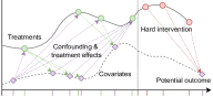
Setup (see Fig. 1): We consider outcomes $Y_{t}\in\mathbb{R}^{d_{y}}$, discrete treatments $A_{t}\in\{0,1\}^{d_{a}}$, and covariates $X_{t}\in\mathbb{R}^{d_{x}}$, where we assume that $X_{t}$ contains $Y_{s}$ for all $s<t$. Without loss of generality, we assume that static covariates are included in $X_{t}$. At time $t$, we let $\pi_{0,t}(A_{t})$ and $\mu_{0,t}(X_{t})$ denote the observational treatment propensity and the covariate distribution, respectively. Both measurement times and treatment times are typically dynamic and do not follow fixed schedules. Rather, both are recorded at arbitrary, irregular timestamps.

To formalize the above in continuous time, we need to be able to model arbitrary timestamps, which increases the complexity compared to the discrete time setting considerably. Following Rytgaard et al. (2022; 2023), we let the counting processes $N_{t}^{x}$ and $N_{t}^{a}$ govern the times at which covariates are measured and at which treatments may be administered, respectively. For both ${z\in\{a,x\}}$, we let $\mathcal{T}_{\tau}^{z}=\{T_{1}^{z},\ldots,T_{N_{\tau}^{z}}^{z}\}$ denote the set of jumping times of the process $N_{t}^{z}$ with $T_{N_{\tau}^{z}}^{z}\leq\tau$. Further, we let $\Lambda_{0}^{z}$ denote the cumulative intensity of $N_{t}^{z}$, and we let $\lambda_{0}^{z}(t)$ denote the corresponding intensity function. Further, we use the short-hand notation $\mathop{}\!\mathrm{d}t=[t,t+\mathop{}\!\mathrm{d}t)$ as in (Gill & Johansen, 1990; Rytgaard et al., 2022). Then, we have that

$\displaystyle\lambda_{0}^{z}(t)\mathop{}\!\mathrm{d}t=\mathop{}\!\mathrm{d}\Lambda_{0}^{z}(t)=\mathbb{E}_{\mathbb{P}_{0}}[N^{z}(\mathop{}\!\mathrm{d}t)]=\mathbb{P}_{0}(N^{z}(\mathop{}\!\mathrm{d}t)=1).$ (1)

Observational likelihood: We write the full observed history up to time $t$ as

$\displaystyle\bar{H}_{t}=\{A_{T_{j}^{a}},X_{T_{j}^{x}},\bar{N}_{t}^{a},\bar{N}_{t}^{x}:\>T_{j}^{a}\in\mathcal{T}_{t}^{a},T_{j}^{x}\in\mathcal{T}_{t}^{x}\}.$ (2)

Then, following (Rytgaard et al., 2022), we can write the observational likelihood of the data $\bar{H}_{\tau}$ via

$\displaystyle\mathop{}\!\mathrm{d}\mathbb{P}_{0}(\bar{H}_{\tau})=$ μ0,0(X0)\prodi\ilimits@s(0,τ]((dΛ0x(sH¯s)μ0,s(XsH¯s))Nx(ds)(1dΛ0x(sH¯s))1Nx(ds)\displaystyle\mu_{0,0}(X_{0})\prodi\ilimits@\limits_{s\in(0,\tau]}\Big{(}\left(\mathop{}\!\mathrm{d}\Lambda_{0}^{x}(s\mid\bar{H}_{s-})\mu_{0,s}(X_{s}\mid\bar{H}_{s-})\right)^{N^{x}(\mathop{}\!\mathrm{d}s)}\left(1-\mathop{}\!\mathrm{d}\Lambda_{0}^{x}(s\mid\bar{H}_{s-})\right)^{1-N^{x}(\mathop{}\!\mathrm{d}s)}
$\displaystyle\times\left(\mathop{}\!\mathrm{d}\Lambda_{0}^{a}(s\mid\bar{H}_{s-})\pi_{0,s}(A_{s}\mid\bar{H}_{s-})\right)^{N^{a}(\mathop{}\!\mathrm{d}s)}\left(1-\mathop{}\!\mathrm{d}\Lambda_{0}^{a}(s\mid\bar{H}_{s-})\right)^{1-N^{a}(\mathop{}\!\mathrm{d}s)}\Big{)},$ (3)

where \prodi\ilimits@\prodi\ilimits@\prodi\ilimits@ is the geometric product integral. Intuitively, the geometric product integral \prodi\ilimits@\prodi\ilimits@\prodi\ilimits@ can be thought of as the infinitesimal limit of the discrete product operator $\Pi$. Importantly, the geometric product integral in Equation 3 is the natural way to describe joint likelihoods in continuous time. For more details, we provide a brief overview of product integration in Supp. B.

Objective: We are interested in predicting the response of the outcome variable $Y_{\tau}$ when intervening on the treatment sequence starting at time $t$, given an observed history $\bar{H}_{t-}=\bar{h}_{t-}$. For this, we adopt the potential outcomes framework (Neyman, 1923; Rubin, 1978). That is, we seek to predict the potential outcome (PO)

𝔼[Yτ[a¯,t,n¯,ta]H¯t=h¯t],𝔼delimited-[]conditionalsubscript𝑌𝜏subscript¯𝑎𝑡superscriptsubscript¯𝑛𝑡𝑎subscript¯𝐻limit-from𝑡subscript¯limit-from𝑡\mathbb{E}\Big{[}Y_{\tau}[\underline{\hbox{\set@color$a$}}_{*,t},\underline{\hbox{\set@color$n$}}_{*,t}^{a}]\,\mid\,\bar{H}_{t-}=\bar{h}_{t-}\Big{]}, (4)

under interventions on both the treatment propensity A¯t=a¯,tsubscript¯𝐴𝑡subscript¯𝑎𝑡\underline{\hbox{\set@color$A$}}_{t}=\underline{\hbox{\set@color$a$}}_{*,t} and the treatment frequency N¯ta=n¯,tasuperscriptsubscript¯𝑁𝑡𝑎superscriptsubscript¯𝑛𝑡𝑎{\underline{\hbox{\set@color$N$}}_{t}^{a}=\underline{\hbox{\set@color$n$}}_{*,t}^{a}}, given the history H¯t=h¯tsubscript¯𝐻limit-from𝑡subscript¯limit-from𝑡\bar{H}_{t-}=\bar{h}_{t-}. Here, the interventions are hard interventions, which is standard in the literature (e.g., Bica et al., 2020; Lim et al., 2018; Melnychuk et al., 2022; Seedat et al., 2022). That is, for st𝑠𝑡s\geq t, we are interested in deterministic interventions of the form

$$A_{s}\sim\pi_{*,s}(A_{s}\mid\bar{H}_{t-}=\bar{h}_{t-})=\mathbbm{1}_{\{A_{s}=a_{*,s}\}},\quad N_{s}^{a}\sim\mathop{}\!\mathrm{d}\Lambda_{*}^{a}(s\mid\bar{H}_{t-}=\bar{h}_{t-})=\mathbbm{1}_{\{t_{*,j}^{a}\}_{j=1}^{J}}(s)\mathop{}\!\mathrm{d}s,$$ (5)

where $a_{*,s}:\mathbb{R}^{+}\to\mathcal{A}$ is a step-wise constant function with jumping points $\{t_{*,j}^{a}\}_{j=1}^{J}$.

Predicting the PO for a treatment sequence is notoriously challenging due to the fundamental problem of causal inference (Imbens & Rubin, 2015). This means, only factual outcomes $Y_{\tau}$ in are observed in the data, but not the potential outcomes when intervening on the treatment. In the following, we first define the interventional distribution for our objective and then ensure identifiability.

Interventional distribution: We now define the interventional distribution for our objective. For this, we rewrite Equation 4 by reweighting $Y_{\tau}$ under the observational distribution $\mathop{}\!\mathrm{d}\mathbb{P}_{0}$. For this, we follow Rytgaard et al. (2023) and first split the likelihood into two separate parts as

d0(H¯τ)=dQ0,G0(H¯τ)=μ0,0(X0)\prodi\ilimits@s(0,τ]dG0,s(H¯s)dQ0,s(H¯s),dsubscript0subscript¯𝐻𝜏dsubscriptsubscript𝑄0subscript𝐺0subscript¯𝐻𝜏subscript𝜇00subscript𝑋0\prodisubscript\ilimits@𝑠0𝜏dsubscript𝐺0𝑠subscript¯𝐻𝑠dsubscript𝑄0𝑠subscript¯𝐻𝑠\displaystyle\mathop{}\!\mathrm{d}\mathbb{P}_{0}(\bar{H}_{\tau})=\mathop{}\!\mathrm{d}\mathbb{P}_{Q_{0},G_{0}}(\bar{H}_{\tau})=\mu_{0,0}(X_{0})\prodi\ilimits@\limits_{s\in(0,\tau]}\mathop{}\!\mathrm{d}G_{0,s}(\bar{H}_{s})\mathop{}\!\mathrm{d}Q_{0,s}(\bar{H}_{s}), (6)

where

$\displaystyle\mathop{}\!\mathrm{d}G_{0,s}(\bar{H}_{s})=\left(\mathop{}\!\mathrm{d}\Lambda_{0}^{a}(s\mid\bar{H}_{s-})\,\pi_{0,s}(A_{s}\mid\bar{H}_{s-})\right)^{N^{a}(\mathop{}\!\mathrm{d}s)}\left(1-\mathop{}\!\mathrm{d}\Lambda_{0}^{a}(s\mid\bar{H}_{s-})\right)^{1-N^{a}(\mathop{}\!\mathrm{d}s)}$ (7)

is the treatment part the we intervene on and where

$\displaystyle\mathop{}\!\mathrm{d}Q_{0,s}(\bar{H}_{s})=\left(\mathop{}\!\mathrm{d}\Lambda_{0}^{x}(s\mid\bar{H}_{s-})\mu_{0,s}(X_{s}\mid\bar{H}_{s-})\right)^{N^{x}(\mathop{}\!\mathrm{d}s)}\left(1-\mathop{}\!\mathrm{d}\Lambda_{0}^{x}(s\mid\bar{H}_{s-})\right)^{1-N^{x}(\mathop{}\!\mathrm{d}s)}$ (8)

remains unchanged. Then, we can write the interventional distribution as

d(H¯τ)=dQ0,G(H¯τ)=μ0,0(X0)\prodi\ilimits@s(0,τ]dG,s(H¯s)dQ0,s(H¯s),dsubscriptsubscript¯𝐻𝜏dsubscriptsubscript𝑄0subscript𝐺subscript¯𝐻𝜏subscript𝜇00subscript𝑋0\prodisubscript\ilimits@𝑠0𝜏dsubscript𝐺𝑠subscript¯𝐻𝑠dsubscript𝑄0𝑠subscript¯𝐻𝑠\displaystyle\mathop{}\!\mathrm{d}\mathbb{P}_{*}(\bar{H}_{\tau})=\mathop{}\!\mathrm{d}\mathbb{P}_{Q_{0},G_{*}}(\bar{H}_{\tau})=\mu_{0,0}(X_{0})\prodi\ilimits@\limits_{s\in(0,\tau]}\mathop{}\!\mathrm{d}G_{*,s}(\bar{H}_{s})\mathop{}\!\mathrm{d}Q_{0,s}(\bar{H}_{s}), (9)

where

$\displaystyle\mathop{}\!\mathrm{d}G_{*,s}(\bar{H}_{s})=\left(\mathop{}\!\mathrm{d}\Lambda_{*}^{a}(s\mid\bar{H}_{s-})\,\pi_{*,s}(A_{s}\mid\bar{H}_{s-})\right)^{N^{a}(\mathop{}\!\mathrm{d}s)}\left(1-\mathop{}\!\mathrm{d}\Lambda_{*}^{a}(s\mid\bar{H}_{s-})\right)^{1-N^{a}(\mathop{}\!\mathrm{d}s)}.$ (10)

Identifiability: To ensure identifiability, we need to make the following assumptions (Lok, 2008; Robins & Hernán, 2009; Rytgaard et al., 2022) that are standard in the literature for predicting potential outcomes over time (e.g., Seedat et al., 2022). (i) Consistency: Given an intervention on the treatment propensity and the frequency [a¯,t,n¯,ta]subscript¯𝑎𝑡superscriptsubscript¯𝑛𝑡𝑎[\underline{\hbox{\set@color$a$}}_{*,t},\underline{\hbox{\set@color$n$}}_{*,t}^{a}], the observed outcome Yτsubscript𝑌𝜏Y_{\tau} coincides with the potential outcome Yτ[a¯,t,n¯,ta]subscript𝑌𝜏subscript¯𝑎𝑡superscriptsubscript¯𝑛𝑡𝑎Y_{\tau}[\underline{\hbox{\set@color$a$}}_{*,t},\underline{\hbox{\set@color$n$}}_{*,t}^{a}] under this intervention. (ii) Positivity: Given any history H¯tsubscript¯𝐻limit-from𝑡\bar{H}_{t-}, the Radon-Nikodỳm derivative dG,t/dG0,tdsubscript𝐺𝑡dsubscript𝐺0𝑡{\mathop{}\!\mathrm{d}G_{*,t}}/{\mathop{}\!\mathrm{d}G_{0,t}} exists. (iii) Unconfoundedness: Given any history H¯tsubscript¯𝐻limit-from𝑡\bar{H}_{t-}, the potential outcome is independent of the treatment assignment probability, that is, Yτ[a¯,t,n¯,ta](A¯t,N¯ta)H¯tperpendicular-tosubscript𝑌𝜏subscript¯𝑎𝑡superscriptsubscript¯𝑛𝑡𝑎conditionalsubscript¯𝐴𝑡superscriptsubscript¯𝑁𝑡𝑎subscript¯𝐻limit-from𝑡Y_{\tau}[\underline{\hbox{\set@color$a$}}_{*,t},\underline{\hbox{\set@color$n$}}_{*,t}^{a}]\perp(\underline{\hbox{\set@color$A$}}_{t},\underline{\hbox{\set@color$N$}}_{t}^{a})\mid\bar{H}_{t-}.

Proposition 1.

Under assumptions (i)–(iii), we can estimate the potential outcome from observational data (i.e., from data sampled under $\mathop{}\!\mathrm{d}\mathbb{P}_{0}$) via inverse propensity weighting, that is,

𝔼[Yτ[a¯,t,n¯,ta]|H¯t=h¯t]=𝔼[Yτ\prodi\ilimits@stWs|(A¯t,N¯ta)=(a¯,t,n¯,a),H¯t=h¯t],𝔼delimited-[]conditionalsubscript𝑌𝜏subscript¯𝑎𝑡superscriptsubscript¯𝑛𝑡𝑎subscript¯𝐻limit-from𝑡subscript¯limit-from𝑡𝔼delimited-[]formulae-sequenceconditionalsubscript𝑌𝜏\prodisubscript\ilimits@𝑠𝑡subscript𝑊𝑠subscript¯𝐴𝑡superscriptsubscript¯𝑁𝑡𝑎subscript¯𝑎𝑡superscriptsubscript¯𝑛𝑎subscript¯𝐻limit-from𝑡subscript¯limit-from𝑡\displaystyle\mathbb{E}\Big{[}Y_{\tau}[\underline{\hbox{\set@color$a$}}_{*,t},\underline{\hbox{\set@color$n$}}_{*,t}^{a}]\;\Big{|}\;\bar{H}_{t-}=\bar{h}_{t-}\Big{]}=\mathbb{E}\Big{[}Y_{\tau}\prodi\ilimits@\limits_{s\geq t}{\color[rgb]{0.0600000000000001,0.46,1}\definecolor[named]{pgfstrokecolor}{rgb}{0.0600000000000001,0.46,1}\pgfsys@color@cmyk@stroke{0.94}{0.54}{0}{0}\pgfsys@color@cmyk@fill{0.94}{0.54}{0}{0}W_{s}}\;\Big{|}\;(\underline{\hbox{\set@color$A$}}_{t},\underline{\hbox{\set@color$N$}}_{t}^{a})=(\underline{\hbox{\set@color$a$}}_{*,t},\underline{\hbox{\set@color$n$}}_{*,}^{a}),\bar{H}_{t-}=\bar{h}_{t-}\Big{]}, (11)

where the inverse propensity weights for $s\geq t$ are defined as

Wsws(H¯s)=dG,s(H¯s)dG0,s(H¯s).subscript𝑊𝑠subscript𝑤𝑠subscript¯𝐻𝑠dsubscript𝐺𝑠subscript¯𝐻𝑠dsubscript𝐺0𝑠subscript¯𝐻𝑠\displaystyle{\color[rgb]{0.0600000000000001,0.46,1}\definecolor[named]{pgfstrokecolor}{rgb}{0.0600000000000001,0.46,1}\pgfsys@color@cmyk@stroke{0.94}{0.54}{0}{0}\pgfsys@color@cmyk@fill{0.94}{0.54}{0}{0}W_{s}}\equiv{\color[rgb]{0.0600000000000001,0.46,1}\definecolor[named]{pgfstrokecolor}{rgb}{0.0600000000000001,0.46,1}\pgfsys@color@cmyk@stroke{0.94}{0.54}{0}{0}\pgfsys@color@cmyk@fill{0.94}{0.54}{0}{0}w_{s}}(\bar{H}_{s})=\frac{\mathop{}\!\mathrm{d}G_{*,s}(\bar{H}_{s})}{\mathop{}\!\mathrm{d}G_{0,s}(\bar{H}_{s})}. (12)
Proof.

See Supp. D. ∎

Proposition 1 is important for the rest of our paper: it tells us that we can predict POs in continuous time from data sampled under $\mathop{}\!\mathrm{d}\mathbb{P}_{0}$. For this, we need to quantify the change in measure from the observational distribution $\mathop{}\!\mathrm{d}\mathbb{P}_{0}$ to the interventional distribution $\mathop{}\!\mathrm{d}\mathbb{P}_{*}$, which is given by Equation 12.

Why is the above task non-trivial? Leveraging the above formulation for predicting potential outcomes is highly challenging due to two reasons: (1) The above formulation is based on a product integral \prodi\ilimits@\prodi\ilimits@\prodi\ilimits@, which is not computationally tractable. $\Rightarrow$ We later derive a novel, tractable formulation where we rewrite Equation 11 using the product operator $\prod$ (Sec. 4.1). (2) Inverse propensity weights Wssubscript𝑊𝑠\color[rgb]{0.0600000000000001,0.46,1}\definecolor[named]{pgfstrokecolor}{rgb}{0.0600000000000001,0.46,1}\pgfsys@color@cmyk@stroke{0.94}{0.54}{0}{0}\pgfsys@color@cmyk@fill{0.94}{0.54}{0}{0}W_{s} may lead to extreme weights and, hence, unstable performance. This is a known issue because settings over time are prone to low overlap (Frauen et al., 2024; Lim et al., 2018). $\Rightarrow$ We later derive novel stabilized weights that are tailored to our continuous time setting (Sec. 4.2).

4 SCIP-Net

In this section, we introduce our SCIP-Net. It is designed to perform proper adjustments for time-varying confounding in continuous time.

Objective: Our objective is to find the optimal parameters222Throughout, we refer to the weights of neural nets as parameters to make the distinction to inverse propensity weights clear. $\hat{\phi}$ of a neural network $m_{\phi}$ via

ϕ^=^italic-ϕabsent\displaystyle\hat{\phi}= argminϕ𝔼[(Yτ[a¯,t,n¯,ta]mϕ(A¯t,N¯ta,H¯t))2|H¯t=h¯t]\displaystyle\operatorname*{arg\,min}_{\phi}\mathbb{E}_{\mathbb{P}_{*}}\left[\Big{(}Y_{\tau}[\underline{\hbox{\set@color$a$}}_{*,t},\underline{\hbox{\set@color$n$}}_{*,t}^{a}]-m_{\phi}(\underline{\hbox{\set@color$A$}}_{t},\underline{\hbox{\set@color$N$}}_{t}^{a},\bar{H}_{t-})\Big{)}^{2}\;\middle|\;\bar{H}_{t-}=\bar{h}_{t-}\right] (13)
=\displaystyle= argminϕ𝔼0[(Yτmϕ(A¯t,N¯ta,H¯t))2\prodi\ilimits@stWs|(A¯t,N¯ta)=(a¯,t,n¯,ta),H¯t=h¯t].subscriptargminitalic-ϕsubscript𝔼subscript0delimited-[]formulae-sequenceconditionalsuperscriptsubscript𝑌𝜏subscript𝑚italic-ϕsubscript¯𝐴𝑡superscriptsubscript¯𝑁𝑡𝑎subscript¯𝐻limit-from𝑡2\prodisubscript\ilimits@𝑠𝑡subscript𝑊𝑠subscript¯𝐴𝑡superscriptsubscript¯𝑁𝑡𝑎subscript¯𝑎𝑡superscriptsubscript¯𝑛𝑡𝑎subscript¯𝐻limit-from𝑡subscript¯limit-from𝑡\displaystyle\operatorname*{arg\,min}_{\phi}\mathbb{E}_{\mathbb{P}_{0}}\Big{[}\Big{(}Y_{\tau}-m_{\phi}(\underline{\hbox{\set@color$A$}}_{t},\underline{\hbox{\set@color$N$}}_{t}^{a},\bar{H}_{t-})\Big{)}^{2}\prodi\ilimits@\limits_{s\geq t}{\color[rgb]{0.0600000000000001,0.46,1}\definecolor[named]{pgfstrokecolor}{rgb}{0.0600000000000001,0.46,1}\pgfsys@color@cmyk@stroke{0.94}{0.54}{0}{0}\pgfsys@color@cmyk@fill{0.94}{0.54}{0}{0}W_{s}}\;\Bigg{|}\;(\underline{\hbox{\set@color$A$}}_{t},\underline{\hbox{\set@color$N$}}_{t}^{a})=(\underline{\hbox{\set@color$a$}}_{*,t},\underline{\hbox{\set@color$n$}}_{*,t}^{a}),\bar{H}_{t-}=\bar{h}_{t-}\Big{]}. (14)

Note that the above objective makes use of inverse propensity weights $W_{s}$. However, these weights suffer from two drawbacks: they are (1) intractable as they rely on product integrals \prodi\ilimits@\prodi\ilimits@\prodi\ilimits@, and (2) they may lead to unstable performance. As a remedy, we (1) derive a tractable expression for this product integral (Sec. 4.1), and we further (2) introduce stabilized weights (Sec. 4.2). Finally, we present our neural architecture (Sec. 4.3) and how to perform inference (Sec. 4.4).

4.1 Rewriting the objective for computational tractability

We now derive a tractable expression to compute our unstabilized weights Wssubscript𝑊𝑠{\color[rgb]{0.0600000000000001,0.46,1}\definecolor[named]{pgfstrokecolor}{rgb}{0.0600000000000001,0.46,1}\pgfsys@color@cmyk@stroke{0.94}{0.54}{0}{0}\pgfsys@color@cmyk@fill{0.94}{0.54}{0}{0}W_{s}} in Equation 12.

Proposition 2.

Let $t_{*,0}^{a}=t$ for notational convenience. The unstabilized weights in Equation 12 satisfy

\prodi\ilimits@stWs|((A¯t,N¯ta)=(a¯,t,n¯,ta),H¯t=h¯t)=conditional\prodisubscript\ilimits@𝑠𝑡subscript𝑊𝑠formulae-sequencesubscript¯𝐴𝑡superscriptsubscript¯𝑁𝑡𝑎subscript¯𝑎𝑡superscriptsubscript¯𝑛𝑡𝑎subscript¯𝐻limit-from𝑡subscript¯limit-from𝑡absent\displaystyle\prodi\ilimits@\limits_{s\geq t}{\color[rgb]{0.0600000000000001,0.46,1}\definecolor[named]{pgfstrokecolor}{rgb}{0.0600000000000001,0.46,1}\pgfsys@color@cmyk@stroke{0.94}{0.54}{0}{0}\pgfsys@color@cmyk@fill{0.94}{0.54}{0}{0}W_{s}}\;\Big{|}\;\Big{(}(\underline{\hbox{\set@color$A$}}_{t},\underline{\hbox{\set@color$N$}}_{t}^{a})=(\underline{\hbox{\set@color$a$}}_{*,t},\underline{\hbox{\set@color$n$}}_{*,t}^{a}),\bar{H}_{t-}=\bar{h}_{t-}\Big{)}= j=1JWt,ja|((A¯t,N¯ta)=(a¯,t,n¯,ta),H¯t=h¯t),conditionalsuperscriptsubscriptproduct𝑗1𝐽subscript𝑊superscriptsubscript𝑡𝑗𝑎formulae-sequencesubscript¯𝐴𝑡superscriptsubscript¯𝑁𝑡𝑎subscript¯𝑎𝑡superscriptsubscript¯𝑛𝑡𝑎subscript¯𝐻limit-from𝑡subscript¯limit-from𝑡\displaystyle\prod_{j=1}^{J}{\color[rgb]{0.0600000000000001,0.46,1}\definecolor[named]{pgfstrokecolor}{rgb}{0.0600000000000001,0.46,1}\pgfsys@color@cmyk@stroke{0.94}{0.54}{0}{0}\pgfsys@color@cmyk@fill{0.94}{0.54}{0}{0}W_{t_{*,j}^{a}}}\;\Big{|}\;\Big{(}(\underline{\hbox{\set@color$A$}}_{t},\underline{\hbox{\set@color$N$}}_{t}^{a})=(\underline{\hbox{\set@color$a$}}_{*,t},\underline{\hbox{\set@color$n$}}_{*,t}^{a}),\bar{H}_{t-}=\bar{h}_{t-}\Big{)}, (15)

where

Wt,ja=exps[t,j1a,t,ja)λ0a(sH¯s)dsλ0a(t,jaH¯t,ja)π0,t,ja(a,t,jaH¯t,ja).subscript𝑊superscriptsubscript𝑡𝑗𝑎subscript𝑠superscriptsubscript𝑡𝑗1𝑎superscriptsubscript𝑡𝑗𝑎superscriptsubscript𝜆0𝑎conditional𝑠subscript¯𝐻limit-from𝑠differential-d𝑠superscriptsubscript𝜆0𝑎conditionalsuperscriptsubscript𝑡𝑗𝑎subscript¯𝐻limit-fromsuperscriptsubscript𝑡𝑗𝑎subscript𝜋0superscriptsubscript𝑡𝑗𝑎conditionalsubscript𝑎superscriptsubscript𝑡𝑗𝑎subscript¯𝐻limit-fromsuperscriptsubscript𝑡𝑗𝑎\displaystyle{\color[rgb]{0.0600000000000001,0.46,1}\definecolor[named]{pgfstrokecolor}{rgb}{0.0600000000000001,0.46,1}\pgfsys@color@cmyk@stroke{0.94}{0.54}{0}{0}\pgfsys@color@cmyk@fill{0.94}{0.54}{0}{0}W_{t_{*,j}^{a}}}=\frac{\exp\int_{s\in[t_{*,j-1}^{a},t_{*,j}^{a})}\lambda_{0}^{a}(s\mid\bar{H}_{s-})\mathop{}\!\mathrm{d}s}{\lambda_{0}^{a}(t_{*,j}^{a}\mid\bar{H}_{t_{*,j}^{a}-})\,\pi_{0,t_{*,j}^{a}}(a_{*,t_{*,j}^{a}}\mid\bar{H}_{t_{*,j}^{a}-})}. (16)
Proof.

See Supp. D. ∎

Proposition 2 has important implications for tractability: Given a history H¯t=h¯tsubscript¯𝐻limit-from𝑡subscript¯limit-from𝑡{\bar{H}_{t-}=\bar{h}_{t-}} and the future sequence of treatments (A¯t,N¯ta)=(a¯,t,n¯,ta)subscript¯𝐴𝑡superscriptsubscript¯𝑁𝑡𝑎subscript¯𝑎𝑡superscriptsubscript¯𝑛𝑡𝑎{(\underline{\hbox{\set@color$A$}}_{t},\underline{\hbox{\set@color$N$}}_{t}^{a})=(\underline{\hbox{\set@color$a$}}_{*,t},\underline{\hbox{\set@color$n$}}_{*,t}^{a})}, the product integral \prodi\ilimits@\prodi\ilimits@\prodi\ilimits@ of the unstabilized inverse propensity weights Wssubscript𝑊𝑠{\color[rgb]{0.0600000000000001,0.46,1}\definecolor[named]{pgfstrokecolor}{rgb}{0.0600000000000001,0.46,1}\pgfsys@color@cmyk@stroke{0.94}{0.54}{0}{0}\pgfsys@color@cmyk@fill{0.94}{0.54}{0}{0}W_{s}} reduces to a finite product product\prod. This product includes both treatment propensities and treatment intensities. In Sec. 4.3, we show how to learn these quantities from data.

Importantly, the unstabilized weights in Equation 16 are already sufficient to adjust for time-varying confounding. However, as they may lead to extreme weights, we now propose stabilized weights.

4.2 Stabilized weights

In the following, we first define our stabilized weights (Def. 1). Then, we show that the optimal parameters $\hat{\phi}$ in Equation 14 are the same, regardless of whether the original, unstabilized inverse propensity weights from above are used or our stabilized weights (Proposition 3). Finally, we present a tractable expression to compute the stabilized weights (Proposition 4).

Definition 1.

For $s\geq t$, let the scaling factor ΞssubscriptΞ𝑠{\color[rgb]{0.72,0,0}\definecolor[named]{pgfstrokecolor}{rgb}{0.72,0,0}\pgfsys@color@cmyk@stroke{0}{0.89}{0.94}{0.28}\pgfsys@color@cmyk@fill{0}{0.89}{0.94}{0.28}\Xi_{s}} be given by the ratio of the marginal transition probabilities of treatment, that is,

Ξsξs(A¯s,N¯sa)=dG0,s(A¯s,N¯sa)dG,s(A¯s,N¯sa).subscriptΞ𝑠subscript𝜉𝑠subscript¯𝐴𝑠superscriptsubscript¯𝑁𝑠𝑎dsubscript𝐺0𝑠subscript¯𝐴𝑠superscriptsubscript¯𝑁𝑠𝑎dsubscript𝐺𝑠subscript¯𝐴𝑠superscriptsubscript¯𝑁𝑠𝑎\displaystyle{\color[rgb]{0.72,0,0}\definecolor[named]{pgfstrokecolor}{rgb}{0.72,0,0}\pgfsys@color@cmyk@stroke{0}{0.89}{0.94}{0.28}\pgfsys@color@cmyk@fill{0}{0.89}{0.94}{0.28}\Xi_{s}}\equiv{\color[rgb]{0.72,0,0}\definecolor[named]{pgfstrokecolor}{rgb}{0.72,0,0}\pgfsys@color@cmyk@stroke{0}{0.89}{0.94}{0.28}\pgfsys@color@cmyk@fill{0}{0.89}{0.94}{0.28}\xi_{s}}(\bar{A}_{s},\bar{N}_{s}^{a})=\frac{\mathop{}\!\mathrm{d}G_{0,s}(\bar{A}_{s},\bar{N}_{s}^{a})}{\mathop{}\!\mathrm{d}G_{*,s}(\bar{A}_{s},\bar{N}_{s}^{a})}. (17)

We define the stabilized weights $\widetilde{W}_{s}$ as

W~s=ΞsWs.subscript~𝑊𝑠subscriptΞ𝑠subscript𝑊𝑠\displaystyle{\color[rgb]{0.72,0,0}\definecolor[named]{pgfstrokecolor}{rgb}{0.72,0,0}\pgfsys@color@cmyk@stroke{0}{0.89}{0.94}{0.28}\pgfsys@color@cmyk@fill{0}{0.89}{0.94}{0.28}\widetilde{W}_{s}}={\color[rgb]{0.72,0,0}\definecolor[named]{pgfstrokecolor}{rgb}{0.72,0,0}\pgfsys@color@cmyk@stroke{0}{0.89}{0.94}{0.28}\pgfsys@color@cmyk@fill{0}{0.89}{0.94}{0.28}\Xi_{s}}{\color[rgb]{0.0600000000000001,0.46,1}\definecolor[named]{pgfstrokecolor}{rgb}{0.0600000000000001,0.46,1}\pgfsys@color@cmyk@stroke{0.94}{0.54}{0}{0}\pgfsys@color@cmyk@fill{0.94}{0.54}{0}{0}W_{s}}. (18)

The idea of stabilized weights (e.g., Lim et al., 2018) is that the marginal transition probabilities ΞssubscriptΞ𝑠{\color[rgb]{0.72,0,0}\definecolor[named]{pgfstrokecolor}{rgb}{0.72,0,0}\pgfsys@color@cmyk@stroke{0}{0.89}{0.94}{0.28}\pgfsys@color@cmyk@fill{0}{0.89}{0.94}{0.28}\Xi_{s}}, on average over the population, downscale the inverse propensity weights. Importantly, the scaling factors are unconditional of the individual history and, therefore, do not change the objective.

To formalize this, we make use of the fact that the optimal parameters in Equation 14 are invariant to multiplicative scaling of the optimization problem with respect to constant scaling factors. We summarize this in the following proposition.

Proposition 3.

The optimal parameters $\hat{\phi}$ in Equation 14 can equivalently be obtained by

ϕ^=argminϕ𝔼0[(Yτmϕ(A¯t,N¯ta,H¯t))2\prodi\ilimits@stW~s|(A¯t,N¯ta)=(a¯,t,n¯,ta),H¯t=h¯t].^italic-ϕsubscriptargminitalic-ϕsubscript𝔼subscript0delimited-[]formulae-sequenceconditionalsuperscriptsubscript𝑌𝜏subscript𝑚italic-ϕsubscript¯𝐴𝑡superscriptsubscript¯𝑁𝑡𝑎subscript¯𝐻limit-from𝑡2\prodisubscript\ilimits@𝑠𝑡subscript~𝑊𝑠subscript¯𝐴𝑡superscriptsubscript¯𝑁𝑡𝑎subscript¯𝑎𝑡superscriptsubscript¯𝑛𝑡𝑎subscript¯𝐻limit-from𝑡subscript¯limit-from𝑡\displaystyle\hat{\phi}=\operatorname*{arg\,min}_{\phi}\mathbb{E}_{\mathbb{P}_{0}}\Bigg{[}\Big{(}Y_{\tau}-m_{\phi}(\underline{\hbox{\set@color$A$}}_{t},\underline{\hbox{\set@color$N$}}_{t}^{a},\bar{H}_{t-})\Big{)}^{2}\prodi\ilimits@\limits_{s\geq t}{\color[rgb]{0.72,0,0}\definecolor[named]{pgfstrokecolor}{rgb}{0.72,0,0}\pgfsys@color@cmyk@stroke{0}{0.89}{0.94}{0.28}\pgfsys@color@cmyk@fill{0}{0.89}{0.94}{0.28}\widetilde{W}_{s}}\;\Bigg{|}\;(\underline{\hbox{\set@color$A$}}_{t},\underline{\hbox{\set@color$N$}}_{t}^{a})=(\underline{\hbox{\set@color$a$}}_{*,t},\underline{\hbox{\set@color$n$}}_{*,t}^{a}),\bar{H}_{t-}=\bar{h}_{t-}\Bigg{]}. (19)
Proof.

See Supp. D. ∎

Proposition 3 guarantees that we can substitute the original, unstabilized weights $W_{s}$ with the stabilized version $\widetilde{W}_{s}$. As the scaling factors $\Xi_{s}$ downscale $W_{s}$, we reduce the risk of receiving extreme inverse propensity weights, and, thus, obtain a more stable objective.

The results from Proposition 3 still rely on product integrals \prodi\ilimits@\prodi\ilimits@\prodi\ilimits@. However, as in Proposition 2, we now derive an equivalent, tractable expression that relies on the product operator $\Pi$ instead.

Proposition 4.

Let $t_{*,0}^{a}=t$ for notational convenience. The scaling factor ΞssubscriptΞ𝑠{\color[rgb]{0.72,0,0}\definecolor[named]{pgfstrokecolor}{rgb}{0.72,0,0}\pgfsys@color@cmyk@stroke{0}{0.89}{0.94}{0.28}\pgfsys@color@cmyk@fill{0}{0.89}{0.94}{0.28}\Xi_{s}} from Equation 17 then satisfies

\prodi\ilimits@stΞs|((A¯t,N¯ta)=(a¯,t,n¯,ta),(A¯t,N¯ta)=(a¯t,n¯ta))conditional\prodisubscript\ilimits@𝑠𝑡subscriptΞ𝑠formulae-sequencesubscript¯𝐴𝑡superscriptsubscript¯𝑁𝑡𝑎subscript¯𝑎𝑡superscriptsubscript¯𝑛𝑡𝑎subscript¯𝐴limit-from𝑡superscriptsubscript¯𝑁limit-from𝑡𝑎subscript¯𝑎limit-from𝑡superscriptsubscript¯𝑛limit-from𝑡𝑎\displaystyle\prodi\ilimits@\limits_{s\geq t}{\color[rgb]{0.72,0,0}\definecolor[named]{pgfstrokecolor}{rgb}{0.72,0,0}\pgfsys@color@cmyk@stroke{0}{0.89}{0.94}{0.28}\pgfsys@color@cmyk@fill{0}{0.89}{0.94}{0.28}\Xi_{s}}\;\Big{|}\;\Big{(}(\underline{\hbox{\set@color$A$}}_{t},\underline{\hbox{\set@color$N$}}_{t}^{a})=(\underline{\hbox{\set@color$a$}}_{*,t},\underline{\hbox{\set@color$n$}}_{*,t}^{a}),(\bar{A}_{t-},\bar{N}_{t-}^{a})=(\bar{a}_{t-},\bar{n}_{t-}^{a})\Big{)} (20)
=\displaystyle= j=1JΞt,ja|((A¯t,N¯ta)=(a¯,t,n¯,ta),(A¯t,N¯ta)=(a¯t,n¯ta)),conditionalsuperscriptsubscriptproduct𝑗1𝐽subscriptΞsuperscriptsubscript𝑡𝑗𝑎formulae-sequencesubscript¯𝐴𝑡superscriptsubscript¯𝑁𝑡𝑎subscript¯𝑎𝑡superscriptsubscript¯𝑛𝑡𝑎subscript¯𝐴limit-from𝑡superscriptsubscript¯𝑁limit-from𝑡𝑎subscript¯𝑎limit-from𝑡superscriptsubscript¯𝑛limit-from𝑡𝑎\displaystyle\prod_{j=1}^{J}{\color[rgb]{0.72,0,0}\definecolor[named]{pgfstrokecolor}{rgb}{0.72,0,0}\pgfsys@color@cmyk@stroke{0}{0.89}{0.94}{0.28}\pgfsys@color@cmyk@fill{0}{0.89}{0.94}{0.28}\Xi_{t_{*,j}^{a}}}\;\Big{|}\;\Big{(}(\underline{\hbox{\set@color$A$}}_{t},\underline{\hbox{\set@color$N$}}_{t}^{a})=(\underline{\hbox{\set@color$a$}}_{*,t},\underline{\hbox{\set@color$n$}}_{*,t}^{a}),(\bar{A}_{t-},\bar{N}_{t-}^{a})=(\bar{a}_{t-},\bar{n}_{t-}^{a})\Big{)}, (21)

where

Ξt,ja=λ0a(t,jaA¯t,ja,N¯t,jaa)π0,t,ja(at,jaA¯t,ja,N¯t,jaa)exps[t,j1a,t,ja)λ0a(sA¯s,N¯sa)ds.subscriptΞsuperscriptsubscript𝑡𝑗𝑎superscriptsubscript𝜆0𝑎conditionalsuperscriptsubscript𝑡𝑗𝑎subscript¯𝐴limit-fromsuperscriptsubscript𝑡𝑗𝑎superscriptsubscript¯𝑁limit-fromsuperscriptsubscript𝑡𝑗𝑎𝑎subscript𝜋0superscriptsubscript𝑡𝑗𝑎conditionalsubscript𝑎superscriptsubscript𝑡𝑗𝑎subscript¯𝐴limit-fromsuperscriptsubscript𝑡𝑗𝑎superscriptsubscript¯𝑁limit-fromsuperscriptsubscript𝑡𝑗𝑎𝑎subscript𝑠superscriptsubscript𝑡𝑗1𝑎superscriptsubscript𝑡𝑗𝑎superscriptsubscript𝜆0𝑎conditional𝑠subscript¯𝐴limit-from𝑠superscriptsubscript¯𝑁limit-from𝑠𝑎differential-d𝑠\displaystyle{\color[rgb]{0.72,0,0}\definecolor[named]{pgfstrokecolor}{rgb}{0.72,0,0}\pgfsys@color@cmyk@stroke{0}{0.89}{0.94}{0.28}\pgfsys@color@cmyk@fill{0}{0.89}{0.94}{0.28}\Xi_{t_{*,j}^{a}}}=\frac{\lambda_{0}^{a}(t_{*,j}^{a}\mid\bar{A}_{t_{*,j}^{a}-},\bar{N}_{t_{*,j}^{a}-}^{a})\,\pi_{0,t_{*,j}^{a}}(a_{t_{*,j}^{a}}\mid\bar{A}_{t_{*,j}^{a}-},\bar{N}_{t_{*,j}^{a}-}^{a})}{\exp\int_{s\in[t_{*,j-1}^{a},t_{*,j}^{a})}\lambda_{0}^{a}(s\mid\bar{A}_{s-},\bar{N}_{s-}^{a})\mathop{}\!\mathrm{d}s}. (22)
Proof.

See Supp. D. ∎

Together, Propositions 2, 3 and 4 yield a (1) tractable objective function that relies on (2) stabilized inverse propensity weights. As we show in the following Sec. 4.3, we can estimate the stabilized weights from data. Thereby, we present our SCIP-Net, which adjusts for time-varying confounding in continuous time.

4.3 Neural architecture

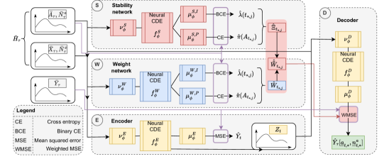
Overview: We now introduce the neural architecture of our SCIP-Net, which consists of four components (see Fig. 2): The S stabilization network learns an estimator of the scaling factors ξs()subscript𝜉𝑠{\color[rgb]{0.72,0,0}\definecolor[named]{pgfstrokecolor}{rgb}{0.72,0,0}\pgfsys@color@cmyk@stroke{0}{0.89}{0.94}{0.28}\pgfsys@color@cmyk@fill{0}{0.89}{0.94}{0.28}\xi_{s}}(\cdot) from Equation 17. The W weight network learns an estimator of the unstabilized inverse propensity weights ws()subscript𝑤𝑠{\color[rgb]{0.0600000000000001,0.46,1}\definecolor[named]{pgfstrokecolor}{rgb}{0.0600000000000001,0.46,1}\pgfsys@color@cmyk@stroke{0.94}{0.54}{0}{0}\pgfsys@color@cmyk@fill{0.94}{0.54}{0}{0}w_{s}}(\cdot) from Equation 12. Combining both, we have an estimator for the stabilized weights w~s()subscript~𝑤𝑠{\color[rgb]{0.72,0,0}\definecolor[named]{pgfstrokecolor}{rgb}{0.72,0,0}\pgfsys@color@cmyk@stroke{0}{0.89}{0.94}{0.28}\pgfsys@color@cmyk@fill{0}{0.89}{0.94}{0.28}\widetilde{w}_{s}}(\cdot) from Equation 18. The E encoder learns a representation of the observed history, which is then passed to the decoder. Finally, the D decoder takes the learned representations and the stabilized inverse propensity weights as input to predict the potential outcomes Y[a¯,t,n¯,ta]𝑌subscript¯𝑎𝑡superscriptsubscript¯𝑛𝑡𝑎Y[\underline{\hbox{\set@color$a$}}_{*,t},\underline{\hbox{\set@color$n$}}_{*,t}^{a}].

Backbones: All components S, W, E, and D use neural controlled differential equations (CDEs) (Kidger et al., 2020; Morrill et al., 2021) as backbones. Neural CDEs have several benefits for our SCIP-Net. First, neural CDEs process data in continuous time. Second, neural CDEs update their hidden states as data becomes available over time. We provide a brief introduction in Supp. C.

Refer to caption
Figure 2: Neural architecture of our SCIP-Net.

In the following, we denote the training samples by {h¯i,τ}i=1nsuperscriptsubscriptsubscript¯𝑖𝜏𝑖1𝑛\{\bar{h}_{i,\tau}\}_{i=1}^{n} and the test samples by {(h¯k,t,a¯,t,n¯,ta)}k=1msuperscriptsubscriptsubscript¯𝑘limit-from𝑡subscript¯𝑎𝑡superscriptsubscript¯𝑛𝑡𝑎𝑘1𝑚\{(\bar{h}_{k,t-},\underline{\hbox{\set@color$a$}}_{*,t},\underline{\hbox{\set@color$n$}}_{*,t}^{a})\}_{k=1}^{m}. Reassuringly, we emphasize that h¯i,t,h¯k,tsubscript¯𝑖limit-from𝑡subscript¯𝑘limit-from𝑡\bar{h}_{i,t-},\bar{h}_{k,t-} are realizations from the observational distribution d0dsubscript0\mathop{}\!\mathrm{d}\mathbb{P}_{0}, whereas (a¯,t,n¯,ta)subscript¯𝑎𝑡superscriptsubscript¯𝑛𝑡𝑎(\underline{\hbox{\set@color$a$}}_{*,t},\underline{\hbox{\set@color$n$}}_{*,t}^{a}) is the interventional treatment sequence.

S

Stability network: The stability network learns an estimator ξ^s()subscript^𝜉𝑠{\color[rgb]{0.72,0,0}\definecolor[named]{pgfstrokecolor}{rgb}{0.72,0,0}\pgfsys@color@cmyk@stroke{0}{0.89}{0.94}{0.28}\pgfsys@color@cmyk@fill{0}{0.89}{0.94}{0.28}\hat{\xi}_{s}}(\cdot) for the scaling factors Ξt,jasubscriptΞsuperscriptsubscript𝑡𝑗𝑎\color[rgb]{0.72,0,0}\definecolor[named]{pgfstrokecolor}{rgb}{0.72,0,0}\pgfsys@color@cmyk@stroke{0}{0.89}{0.94}{0.28}\pgfsys@color@cmyk@fill{0}{0.89}{0.94}{0.28}{\Xi_{t_{*,j}^{a}}} from Proposition 4. It consists of a linear input layer $\nu_{\phi}^{S}$, a neural vector field $f_{\phi}^{S}$, and two linear output layers $\mu_{\phi}^{S,I}$ and $\mu_{\phi}^{S,P}$, which estimate the treatment intensity and propensity, respectively.

Training: The stability network receives treatment decisions and treatment times $(\bar{A}_{\tau},\bar{N}_{\tau}^{a})=(\bar{a}_{i,\tau},\bar{n}_{i,\tau}^{a})$. We distinguish two cases. For $0\leq t<\tau$, the latent representation $z_{i,t}^{S}$ evolves as

$\displaystyle z_{i,t}^{S}=z_{i,0}^{S}+\int_{0}^{t}f_{\phi}^{S}(z_{i,s},s)\mathop{}\!\mathrm{d}[{a}_{i,s-},{n}_{i,s-}^{a}],$ (23)

where $\mathop{}\!\mathrm{d}[{a}_{i,s-},{n}_{i,s-}^{a}]$ denotes Riemann-Stieltjes integration with respect to the control path and ${z_{i,0}^{S}=\nu_{\phi}^{S}({a}_{i,0},{n}_{i,0}^{a})}$. Case (1): The latent representation is then passed to the intensity layer $\mu_{\phi}^{S,I}$ in order to predict the probability whether a treatment decision is made at time $t$. For this, our SCIP-Net optimizes the binary cross entropy (BCE) loss

$\displaystyle\mathcal{L}_{t}^{S,I}(\phi)=\text{BCE}\Big{(}\mu_{\phi}^{S,I}(z_{i,t}^{S}),\mathop{}\!\mathrm{d}{n}_{i,t}^{a}\Big{)}.$ (24)

Thereby, the intensity layer $\mu_{\phi}^{S,I}$ learns an estimator of the treatment intensity function via

$\displaystyle\hat{\lambda}_{0}^{a}(t\mid\bar{A}_{t-},\bar{N}_{t-}^{a})=\mu_{\phi}^{S,I}(Z_{t}^{S}).$ (25)

Case (2): If a treatment decision is made at time $T_{j}^{a}=t_{i,j}^{a}$, the latent representation is additionally passed through the propensity output layer $\mu_{\phi}^{S,P}$ to predict which treatment is administered. For this, our SCIP-Net minimizes the cross entropy (CE) loss

$\displaystyle\mathcal{L}_{j}^{S,P}(\phi)=\text{CE}\Big{(}\mu_{\phi}^{S,P}(z_{i,t_{i,j}^{a}}^{S}),{a}_{i,t_{i,j}^{a}}\Big{)},$ (26)

Hence, the propensity layer learns an estimator of the propensity score via

$\displaystyle\hat{\pi}_{0}^{a}(a_{t}\mid\bar{A}_{t-},\bar{N}_{t-}^{a})=\mu_{\phi}^{S,P}(Z_{t}^{S}).$ (27)

Scaling factor: After training, the stability network again receives the training samples ${(\bar{A}_{\tau},\bar{N}_{\tau}^{a})=(\bar{a}_{i,\tau},\bar{n}_{i,\tau}^{a})}$. Following Proposition 4, it then computes

\prodi\ilimits@stξ^s(a¯i,s,n¯i,sa)\prodisubscript\ilimits@𝑠𝑡subscript^𝜉𝑠subscript¯𝑎𝑖𝑠superscriptsubscript¯𝑛𝑖𝑠𝑎\displaystyle\prodi\ilimits@\limits_{s\geq t}{\color[rgb]{0.72,0,0}\definecolor[named]{pgfstrokecolor}{rgb}{0.72,0,0}\pgfsys@color@cmyk@stroke{0}{0.89}{0.94}{0.28}\pgfsys@color@cmyk@fill{0}{0.89}{0.94}{0.28}{\hat{\xi}_{s}}}(\bar{a}_{i,s},\bar{n}_{i,s}^{a}) (28)
$\displaystyle=\prod_{j=1}^{J}\frac{\hat{\lambda}_{0}^{a}(t_{i,j}^{a}\mid\bar{A}_{t_{i,j}^{a}-}=\bar{a}_{i,t_{i,j}^{a}-},\bar{N}_{t_{i,j}^{a}-}^{a}=\bar{n}_{i,t_{i,j}^{a}-}^{a})\,\hat{\pi}_{0,t_{i,j}^{a}}(a_{t_{i,j}^{a}}\mid\bar{A}_{t_{i,j}^{a}-}=\bar{a}_{i,t_{i,j}^{a}-},\bar{N}_{t_{i,j}^{a}-}^{a}=\bar{n}_{i,t_{i,j}^{a}-}^{a})}{\exp\int_{s\in[t_{i,j-1}^{a},t_{i,j}^{a})}\hat{\lambda}_{0}^{a}(s\mid\bar{A}_{s-}=\bar{a}_{i,s-},\bar{N}_{s}^{a}=\bar{n}_{i,s-}^{a})\mathop{}\!\mathrm{d}s},$

where we can use an arbitrary quadrature scheme to compute the integral in the denominator.

W

Weight network: The weight network learns an estimator w^s()subscript^𝑤𝑠{\color[rgb]{0.0600000000000001,0.46,1}\definecolor[named]{pgfstrokecolor}{rgb}{0.0600000000000001,0.46,1}\pgfsys@color@cmyk@stroke{0.94}{0.54}{0}{0}\pgfsys@color@cmyk@fill{0.94}{0.54}{0}{0}\hat{w}_{s}}(\cdot) for the unstabilized weights Wt,jasubscript𝑊superscriptsubscript𝑡𝑗𝑎\color[rgb]{0.0600000000000001,0.46,1}\definecolor[named]{pgfstrokecolor}{rgb}{0.0600000000000001,0.46,1}\pgfsys@color@cmyk@stroke{0.94}{0.54}{0}{0}\pgfsys@color@cmyk@fill{0.94}{0.54}{0}{0}{W_{t_{*,j}^{a}}} from Proposition 2. It also consists of a linear input layer $\nu_{\phi}^{W}$, a neural vector field $f_{\phi}^{W}$, and two linear output layers $\mu_{\phi}^{W,I}$ and $\mu_{\phi}^{W,P}$, which are trained to estimate the treatment intensity and propensity, respectively.

Training: The weight network receives samples $\bar{H}_{\tau}=\bar{h}_{i,\tau}$. After $h_{i,0}$ is transformed into $z_{i,0}^{W}$ via $\nu_{\phi}^{W}$, the latent state $z_{i,t}^{W}$ of the weight network evolves as

$\displaystyle\mathop{}\!\mathrm{d}z_{i,t}^{W}=z_{i,0}^{W}+\int_{0}^{t}f_{\phi}^{W}(z_{i,s}^{W},s)\mathop{}\!\mathrm{d}[{h}_{i,s-}],$ (29)

where $\mathop{}\!\mathrm{d}[{h}_{i,s-}]$ denotes Riemann-Stieltjes integration w.r.t. the control path. Case (1): As for the stability network, the weight network predicts the probability of a treatment decision at time $t$ through the intensity layer $\mu_{\phi}^{W,I}$ via

$\displaystyle\mathcal{L}_{t}^{W,I}=\text{BCE}\Big{(}\mu_{\phi}^{W,I}(z_{i,t}^{W}),\mathop{}\!\mathrm{d}{n}_{i,t}^{a}\Big{)},$ (30)

and, hence, learns an estimator of the treatment intensity function via

$\displaystyle\hat{\lambda}_{0}^{a}(t\mid\bar{H}_{t-})=\mu_{\phi}^{T,I}(Z_{t}^{W}).$ (31)

Case (2): If a treatment decision is made at time $T_{j}^{a}=t_{i,j}^{a}$, the latent state is also passed through the propensity layer $\mu_{\phi}^{W,P}$ and jointly trained via

$\displaystyle\mathcal{L}_{j}^{W,P}=\text{CE}\Big{(}\mu_{\phi}^{W,P}(z_{i,t_{i,j}^{a}}^{W}),{a}_{i,t_{i,j}^{a}}\Big{)},$ (32)

such that our SCIP-Net learns an estimator of the propensity score as

$\displaystyle\hat{\pi}_{0}^{a}(a_{t}\mid\bar{H}_{t-})=\mu_{\phi}^{W,P}(Z_{t}^{W}).$ (33)

Inverse propensity weight: After training, the weight network again receives the training samples $\bar{H}_{\tau}=\bar{h}_{i,\tau}$ and estimates the unstabilized inverse propensity weights according to Proposition 2 via

\prodi\ilimits@stw^s(h¯i,s)=j=1Jexps[ti,j1a,ti,ja)λ^0a(sH¯s=h¯i,s)dsλ^0a(ti,jaH¯ti,ja=h¯ti,ja)π^0,ti,ja(ai,ti,jaH¯t,ja=h¯ti,ja).\prodisubscript\ilimits@𝑠𝑡subscript^𝑤𝑠subscript¯𝑖limit-from𝑠superscriptsubscriptproduct𝑗1𝐽subscript𝑠superscriptsubscript𝑡𝑖𝑗1𝑎superscriptsubscript𝑡𝑖𝑗𝑎superscriptsubscript^𝜆0𝑎conditional𝑠subscript¯𝐻limit-from𝑠subscript¯𝑖limit-from𝑠differential-d𝑠superscriptsubscript^𝜆0𝑎conditionalsuperscriptsubscript𝑡𝑖𝑗𝑎subscript¯𝐻limit-fromsuperscriptsubscript𝑡𝑖𝑗𝑎subscript¯limit-fromsuperscriptsubscript𝑡𝑖𝑗𝑎subscript^𝜋0superscriptsubscript𝑡𝑖𝑗𝑎conditionalsubscript𝑎𝑖superscriptsubscript𝑡𝑖𝑗𝑎subscript¯𝐻limit-fromsuperscriptsubscript𝑡𝑗𝑎subscript¯limit-fromsuperscriptsubscript𝑡𝑖𝑗𝑎\displaystyle\prodi\ilimits@\limits_{s\geq t}{\color[rgb]{0.0600000000000001,0.46,1}\definecolor[named]{pgfstrokecolor}{rgb}{0.0600000000000001,0.46,1}\pgfsys@color@cmyk@stroke{0.94}{0.54}{0}{0}\pgfsys@color@cmyk@fill{0.94}{0.54}{0}{0}\hat{w}_{s}}(\bar{h}_{i,s-})=\prod_{j=1}^{J}\frac{\exp\int_{s\in[t_{i,j-1}^{a},t_{i,j}^{a})}\hat{\lambda}_{0}^{a}(s\mid\bar{H}_{s-}=\bar{h}_{i,s-})\mathop{}\!\mathrm{d}s}{\hat{\lambda}_{0}^{a}(t_{i,j}^{a}\mid\bar{H}_{t_{i,j}^{a}-}=\bar{h}_{t_{i,j}^{a}-})\,\hat{\pi}_{0,t_{i,j}^{a}}(a_{i,t_{i,j}^{a}}\mid\bar{H}_{t_{*,j}^{a}-}=\bar{h}_{t_{i,j}^{a}-})}. (34)
E

Encoder: The encoder computes a latent representation of the history, which is then passed to the decoder. It consists of a linear input layer $\nu_{\phi}^{E}$, a neural vector field $f_{\phi}^{E}$, and an output layer $\mu_{\phi}^{E}$.

Training: The encoder receives samples $\bar{H}_{\tau}=\bar{h}_{i,\tau}$. First, it transforms $\bar{h}_{i,0}$ into $z_{i,0}^{E}$ via $\nu_{\phi}^{E}$. The latent state $z_{i,t}^{E}$ then evolves according to

$\displaystyle z_{i,t}^{E}=z_{i,0}^{E}+\int_{0}^{t}f_{\phi}^{E}(z_{i,s}^{E},s)\mathop{}\!\mathrm{d}[{h}_{i,s-}],$ (35)

where $\mathop{}\!\mathrm{d}[{h}_{i,s-}]$ denotes Riemann-Stieltjes integration w.r.t. the control path. At jumping times $n_{i,t}^{x}$, we pass the latent state $z_{i,t}$ to the encoder output layer $\mu_{\phi}^{E}$ and minimize the mean squared error (MSE) loss for outcomes at the jumping times via

$\displaystyle\mathcal{L}_{t}^{E}=\text{MSE}\Big{(}\mu_{\phi}^{E}(z_{i,t}^{E},a_{i,t}),{y}_{i,t}\Big{)}.$ (36)
D

Decoder: The decoder receives as input: (i) the encoded history of the encoder and (ii) the future sequence of treatments. Then, it outputs a prediction of the potential outcomes by adjusting for time-varying confounding. It has a linear input layer $\nu_{\phi}^{D}$, a neural vector field $f_{\phi}^{D}$ and an output layer $\mu_{\phi}^{D}$.

Training: During training, the decoder receives the final latent representation zi,tEsuperscriptsubscript𝑧𝑖𝑡𝐸z_{i,t}^{E} of the encoder as well as the observed treatments (A¯t,N¯ta)=(a¯i,t,n¯i,ta)subscript¯𝐴𝑡superscriptsubscript¯𝑁𝑡𝑎subscript¯𝑎𝑖𝑡superscriptsubscript¯𝑛𝑖𝑡𝑎(\underline{\hbox{\set@color$A$}}_{t},\underline{\hbox{\set@color$N$}}_{t}^{a})=(\underline{\hbox{\set@color$a$}}_{i,t},\underline{\hbox{\set@color$n$}}_{i,t}^{a}). It then transforms the encoder representation through zi,tD=νϕD(zi,tE)superscriptsubscript𝑧𝑖𝑡𝐷superscriptsubscript𝜈italic-ϕ𝐷superscriptsubscript𝑧𝑖𝑡𝐸z_{i,t}^{D}=\nu_{\phi}^{D}(z_{i,t}^{E}) and computes

$\displaystyle z_{i,\tau}^{D}=z_{i,t}^{D}+\int_{t}^{\tau}f_{\phi}^{D}(z_{i,s}^{D},s)\mathop{}\!\mathrm{d}[{a}_{i,s-},n_{i,s-}^{a}],$ (37)

where $\mathop{}\!\mathrm{d}[{a}_{i,s-},n_{i,s-}^{a}]$ denotes Riemann-Stieltjes integration w.r.t. the control path. At time $\tau$, we pass $z_{i,\tau}^{D}$ through the linear output layer $\mu_{\phi}^{D}$. Importantly, the decoder is trained by minimizing the MSE loss weighted by the stabilized weights, i.e.,

τD=j=1Jw~^ti,jaMSE(μϕD(zi,τD,ai,τ),yi,τ),superscriptsubscript𝜏𝐷superscriptsubscriptproduct𝑗1𝐽subscript^~𝑤superscriptsubscript𝑡𝑖𝑗𝑎MSEsuperscriptsubscript𝜇italic-ϕ𝐷superscriptsubscript𝑧𝑖𝜏𝐷subscript𝑎𝑖𝜏subscript𝑦𝑖𝜏\displaystyle\mathcal{L}_{\tau}^{D}=\prod_{j=1}^{J}{\color[rgb]{0.72,0,0}\definecolor[named]{pgfstrokecolor}{rgb}{0.72,0,0}\pgfsys@color@cmyk@stroke{0}{0.89}{0.94}{0.28}\pgfsys@color@cmyk@fill{0}{0.89}{0.94}{0.28}\hat{\widetilde{w}}_{t_{i,j}^{a}}}\text{MSE}\Big{(}\mu_{\phi}^{D}(z_{i,\tau}^{D},a_{i,\tau}),{y}_{i,\tau}\Big{)}, (38)

where

w~^ti,jaw~^ti,ja(h¯i,ti,ja)=ξ^ti,ja(a¯i,ti,ja,n¯i,ti,jaa)w^ti,ja(h¯i,ti,ja),subscript^~𝑤superscriptsubscript𝑡𝑖𝑗𝑎subscript^~𝑤superscriptsubscript𝑡𝑖𝑗𝑎subscript¯𝑖superscriptsubscript𝑡𝑖𝑗𝑎subscript^𝜉superscriptsubscript𝑡𝑖𝑗𝑎subscript¯𝑎𝑖superscriptsubscript𝑡𝑖𝑗𝑎superscriptsubscript¯𝑛𝑖superscriptsubscript𝑡𝑖𝑗𝑎𝑎subscript^𝑤superscriptsubscript𝑡𝑖𝑗𝑎subscript¯𝑖superscriptsubscript𝑡𝑖𝑗𝑎\displaystyle{\color[rgb]{0.72,0,0}\definecolor[named]{pgfstrokecolor}{rgb}{0.72,0,0}\pgfsys@color@cmyk@stroke{0}{0.89}{0.94}{0.28}\pgfsys@color@cmyk@fill{0}{0.89}{0.94}{0.28}\hat{\widetilde{w}}_{t_{i,j}^{a}}}\equiv{\color[rgb]{0.72,0,0}\definecolor[named]{pgfstrokecolor}{rgb}{0.72,0,0}\pgfsys@color@cmyk@stroke{0}{0.89}{0.94}{0.28}\pgfsys@color@cmyk@fill{0}{0.89}{0.94}{0.28}\hat{\widetilde{w}}_{t_{i,j}^{a}}}(\bar{h}_{i,t_{i,j}^{a}})={\color[rgb]{0.72,0,0}\definecolor[named]{pgfstrokecolor}{rgb}{0.72,0,0}\pgfsys@color@cmyk@stroke{0}{0.89}{0.94}{0.28}\pgfsys@color@cmyk@fill{0}{0.89}{0.94}{0.28}\hat{\xi}_{t_{i,j}^{a}}}(\bar{a}_{i,t_{i,j}^{a}},\bar{n}_{i,t_{i,j}^{a}}^{a}){\color[rgb]{0.0600000000000001,0.46,1}\definecolor[named]{pgfstrokecolor}{rgb}{0.0600000000000001,0.46,1}\pgfsys@color@cmyk@stroke{0.94}{0.54}{0}{0}\pgfsys@color@cmyk@fill{0.94}{0.54}{0}{0}\hat{w}_{t_{i,j}^{a}}}(\bar{h}_{i,t_{i,j}^{a}}), (39)

using the stability network ξ^s()subscript^𝜉𝑠{\color[rgb]{0.72,0,0}\definecolor[named]{pgfstrokecolor}{rgb}{0.72,0,0}\pgfsys@color@cmyk@stroke{0}{0.89}{0.94}{0.28}\pgfsys@color@cmyk@fill{0}{0.89}{0.94}{0.28}\hat{\xi}_{s}}(\cdot) and the weight network w^s()subscript^𝑤𝑠{\color[rgb]{0.0600000000000001,0.46,1}\definecolor[named]{pgfstrokecolor}{rgb}{0.0600000000000001,0.46,1}\pgfsys@color@cmyk@stroke{0.94}{0.54}{0}{0}\pgfsys@color@cmyk@fill{0.94}{0.54}{0}{0}\hat{w}_{s}}(\cdot), respectively. By Proposition 3, we thereby target the optimal model parameters $\hat{\phi}$ which, unlike existing methods, explicitly adjust for time-varying confounding in continuous time.

4.4 Inference

In order to predict potential outcomes for an observed history H¯t=h¯k,tsubscript¯𝐻limit-from𝑡subscript¯𝑘limit-from𝑡\bar{H}_{t-}=\bar{h}_{k,t-} and a future sequence of treatments (A¯t,N¯ta)=(a¯,t,n¯,ta)subscript¯𝐴𝑡superscriptsubscript¯𝑁𝑡𝑎subscript¯𝑎𝑡superscriptsubscript¯𝑛𝑡𝑎(\underline{\hbox{\set@color$A$}}_{t},\underline{\hbox{\set@color$N$}}_{t}^{a})=(\underline{\hbox{\set@color$a$}}_{*,t},\underline{\hbox{\set@color$n$}}_{*,t}^{a}), we first encode the history via

$\displaystyle z_{k,t}^{E}=z_{k,0}^{E}+\int_{0}^{t}f_{\phi}^{E}(z_{k,s}^{E},s)\mathop{}\!\mathrm{d}[{h}_{k,s-}].$ (40)

This latent representation is then passed to the decoder along with (a¯,t,n¯,ta)subscript¯𝑎𝑡superscriptsubscript¯𝑛𝑡𝑎(\underline{\hbox{\set@color$a$}}_{*,t},\underline{\hbox{\set@color$n$}}_{*,t}^{a}) in order to compute the final representation

$\displaystyle z_{k,\tau}^{D}=\nu_{\phi}^{D}(z_{k,t}^{E})+\int_{t}^{\tau}f_{\phi}^{D}(z_{k,s}^{D},s)\mathop{}\!\mathrm{d}[{a}_{*,s-},n_{*,s-}^{a}].$ (41)

Finally, the output layer $\mu_{\phi}^{D}$ of the decoder is used to predict the potential outcome at time $\tau$, given the history $\bar{H}_{t-}=\bar{h}_{k,t-}$, via

𝔼^[Yτ[a¯,t,n¯,ta]|H¯t=h¯k,t]=μϕD(zk,τD,ak,τ).^𝔼delimited-[]conditionalsubscript𝑌𝜏subscript¯𝑎𝑡superscriptsubscript¯𝑛𝑡𝑎subscript¯𝐻limit-from𝑡subscript¯𝑘limit-from𝑡superscriptsubscript𝜇italic-ϕ𝐷superscriptsubscript𝑧𝑘𝜏𝐷subscript𝑎𝑘𝜏\displaystyle\hat{\mathbb{E}}\Big{[}Y_{\tau}[\underline{\hbox{\set@color$a$}}_{*,t},\underline{\hbox{\set@color$n$}}_{*,t}^{a}]\;\big{|}\;\bar{H}_{t-}=\bar{h}_{k,t-}\Big{]}=\mu_{\phi}^{D}(z_{k,\tau}^{D},a_{k,\tau}). (42)

5 Numerical Experiments

Baselines: We now demonstrate the performance of our SCIP-Net against key neural baselines for predicting potential outcomes over time (see Table 1). Importantly, our choice of baselines and datasets is consistent with prior literature (e.g., Bica et al., 2020; Lim et al., 2018; Melnychuk et al., 2022; Seedat et al., 2022). Further, we report the performance of the CIP-Net ablation, where we directly train the decoder with the unstabilized weights. This allows us to understand the performance gain of our stabilized weights. Note that the CIP-Net ablation is still a new method (as no other neural method performs proper adjustments for time-varying confounding in continuous time).

Datasets: We use a (i) synthetic dataset based on a tumor growth model (Geng et al., 2017), and a (ii) semi-synthetic dataset based on the MIMIC-III dataset (Johnson et al., 2016). For both datasets, the outcomes are simulated, so that we have access to the ground-truth potential outcomes, which allows us to compare the performance in terms of root mean squared error (RMSE). We report the mean $\pm$ the standard deviation over five runs with different seeds. We perform rigorous hyperparameter tuning for all baselines to ensure a fair comparison (see Supp. F).

Tumor growth data: Tumor growth models are widely used for predicting potential outcomes over time. Here, we follow Vanderschueren et al. (2023), where observation times are at arbitrary, irregular timestamps. Below, we vary the prediction horizons (up to three days ahead) and the confounding strength. We provide details in Supp. E.1.

Refer to caption
(a) One day ahead prediction
Refer to caption
(b) Two days ahead prediction
Refer to caption
(c) Three days ahead prediction
Figure 3: Performance for the tumor growth model. We compare different forecast horizons and different confound strengths. Shown is the average RMSE over five seeds. Evidently, our proposed SCIP-Net performs best, followed by our CIP-Net ablation.

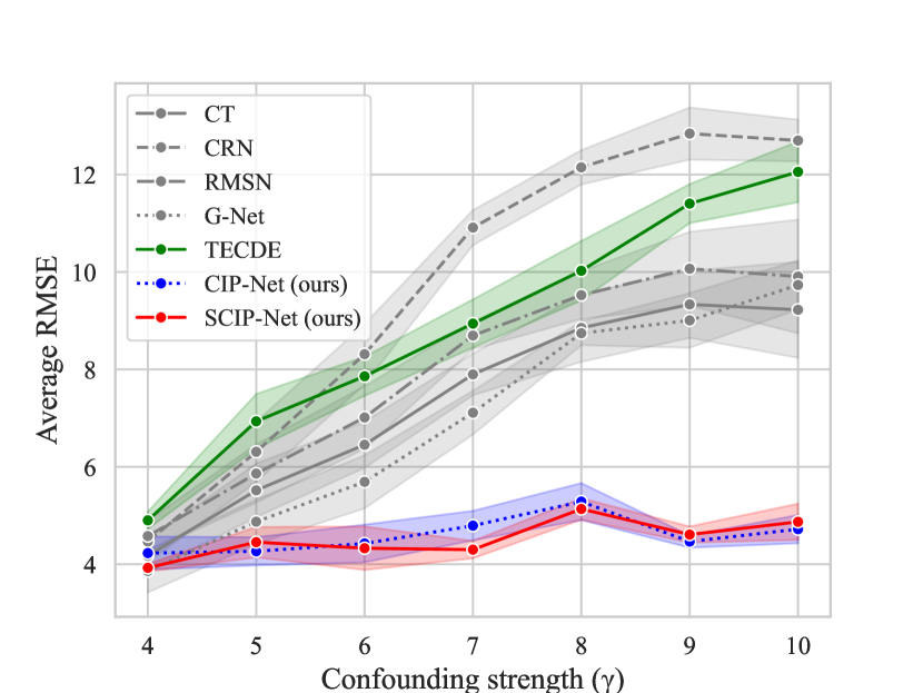
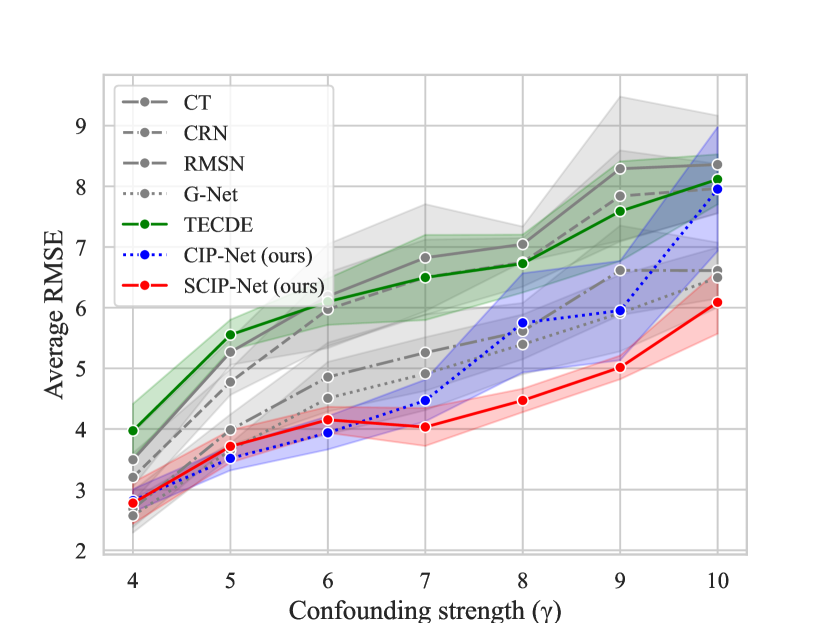
The results are in Fig. 3. We make the following observations: (1) Our proposed SCIP-Net performs best. The performance gains become especially obvious for increasing levels of time-varying confounding because ours is the first method to perform proper adjustments in continuous time. (2) Our proposed SCIP-Net performs more robust than the CIP-Net ablation, which demonstrates the effectiveness of our stabilized weights over the unstabilized weights. The stabilized weights help predicting more accurately especially for larger prediction horizons and strong confounding. (3) Nevertheless, our CIP-Net, has a competitive performance. (4) The only baseline designed for continuous time is TE-CDE (shown in green), which we outperform by a large margin. (5) All other neural baselines are instead designed for discrete time (shown in gray) and are outperformed clearly.

$\Rightarrow$ Takeaway: Our SCIP-Net performs best due to (i) proper adjustments for time-varying confounding in continuous time and (ii) stabilized weights.

MIMIC-III data: Our experiments are based on the MIMIC-III extract from Wang et al. (2020). Here, we use real-world covariates at irregular measurement timestamps, and then simulate treatments and outcomes, respectively. This is done analogous to (Melnychuk et al., 2022), such that we have access to the ground-truth potential outcomes. For the outcome variable, we additionally apply a random observation mask in order to mimic observations at arbitrary, irregular timestamps. We provide more details in Supp. E.2.

Prediction window CT CRN RMSNs G-Net TE-CDE CIP-Net (ours) SCIP-Net (ours) Rel. improvement
$(\tau-t)=1$ hours $1.052\pm 0.069$ $1.049\pm 0.065$ $1.075\pm 0.074$ $1.021\pm 0.069$ $0.915\pm 0.025$ $\bm{0.876\pm 0.041}$ $0.877\pm 0.044$ $+4.1\%$
$(\tau-t)=2$ hours $1.196\pm 0.272$ $1.088\pm 0.374$ $1.130\pm 0.274$ $1.095\pm 0.335$ $0.784\pm 0.145$ $0.785\pm 0.117$ $\bm{0.634\pm 0.148}$ $+19.1\%$
$(\tau-t)=3$ hours $1.444\pm 0.232$ $1.262\pm 0.355$ $1.300\pm 0.304$ $1.330\pm 0.198$ $1.240\pm 0.242$ $1.291\pm 0.400$ $\bm{1.089\pm 0.322}$ $+12.2\%$
Table 2: Performance for MIMIC-III. Reported is the average RMSE over five seeds. We highlight the relative improvement of our SCIP-Net over existing baselines. The results again confirm the effectiveness of our proposed method as our proposed SCIP-Net performs best.

Table 2 shows the results for different prediction windows. (1) Our SCIP-Net has the lowest error among all methods and performs thus again best. (2) Our CIP-Net ablation, which is a new method in itself, again has highly competitive performance. (3) Yet, the ablation shows that using stabilized weights as in SCIP-Net (as opposed to the unstabilized weights as in CIP-Net) makes a large contribution to the overall performance.

$\Rightarrow$ Takeaway: Both the adjustments for time-varying confounding in continuous and the stabilized weights lead to the performance gains. Further, the results demonstrate the applicability and relevance of our method to medical datasets.

Conclusion: To the best of our knowledge, SCIP-Net is the first neural method for predicting potential outcomes through proper adjustments for time-varying confounding in continuous time. For this, we first derive a tractable expression for inverse propensity weighting in continuous time. Then, we propose stabilized weights in continuous time to stabilize the training objective. Our experiments show that our SCIP-Net has clear benefits over existing baselines when observation times and treatment times take place at arbitrary, irregular timestamps.

References

  • Allam et al. (2021) Ahmed Allam, Stefan Feuerriegel, Michael Rebhan, and Michael Krauthammer. Analyzing patient trajectories with artificial intelligence. Journal of Medical Internet Research, 23(12):e29812, 2021.
  • Bang & Robins (2005) Heejung Bang and James M. Robins. Doubly robust estimation in missing data and causal inference models. Biometrics, 61(4):962–973, 2005.
  • Bashirov et al. (2011) Agamirza E. Bashirov, Emine Mısırlı, Yücel Tandoğdu, and Ali Özyapıcı. On modeling with multiplicative differential equations. Applied Mathematics - A Journal of Chinese Universities, 26:425 – 438, 2011.
  • Battalio et al. (2021) Samuel L. Battalio, David E. Conroy, Walter Dempsey, Peng Liao, Marianne Menictas, Susan Murphy, Inbal Nahum-Shani, Tianchen Qian, Santosh Kumar, and Bonnie Spring. Sense2Stop: A micro-randomized trial using wearable sensors to optimize a just-in-time-adaptive stress management intervention for smoking relapse prevention. Contemporary Clinical Trials, 109:106534, 2021.
  • Bica et al. (2020) Ioana Bica, Ahmed M. Alaa, James Jordon, and Mihaela van der Schaar. Estimating counterfactual treatment outcomes over time through adversarially balanced representations. In ICLR, 2020.
  • Bica et al. (2021) Ioana Bica, Ahmed M. Alaa, Craig Lambert, and Mihaela van der Schaar. From real-world patient data to individualized treatment effects using machine learning: Current and future methods to address underlying challenges. Clinical Pharmacology and Therapeutics, 109(1):87–100, 2021.
  • Chen et al. (2018) Ricky T. Q. Chen, Yulia Rubanova, Jesse Bettencourt, and David Duvenaud. Neural ordinary differential equations. In NeurIPS, 2018.
  • Curth & van der Schaar (2021) Alicia Curth and Mihaela van der Schaar. Nonparametric estimation of heterogeneous treatment effects: From theory to learning algorithms. In AISTATS, 2021.
  • Feuerriegel et al. (2024) Stefan Feuerriegel, Dennis Frauen, Valentyn Melnychuk, Jonas Schweisthal, Konstantin Hess, Alicia Curth, Stefan Bauer, Niki Kilbertus, Isaac S. Kohane, and Mihaela van der Schaar. Causal machine learning for predicting treatment outcomes. Nature Medicine, 30:958–968, 2024.
  • Frauen et al. (2023) Dennis Frauen, Tobias Hatt, Valentyn Melnychuk, and Stefan Feuerriegel. Estimating average causal effects from patient trajectories. In AAAI, 2023.
  • Frauen et al. (2024) Dennis Frauen, Konstantin Hess, and Stefan Feuerriegel. Model-agnostic meta-learners for estimating heterogeneous treatment effects over time. arXiv preprint, 2024.
  • Geng et al. (2017) Changran Geng, Harald Paganetti, and Clemens Grassberger. Prediction of treatment response for combined chemo- and radiation therapy for non-small cell lung cancer patients using a bio-mathematical model. Scientific Reports, 7(1):13542, 2017.
  • Gill & Johansen (1990) Richard D. Gill and Soren Johansen. A survey of product-integration with a view toward application in survival analysis. Annals of Statistics, 18(4), 1990.
  • Haber & Ruthotto (2018) Eldad Haber and Lars Ruthotto. Stable architectures for deep neural networks. Inverse Problems, 34(1):014004, 2018.
  • Hatt & Feuerriegel (2021a) Tobias Hatt and Stefan Feuerriegel. Sequential deconfounding for causal inference with unobserved confounders. arXiv preprint, 2021a.
  • Hatt & Feuerriegel (2021b) Tobias Hatt and Stefan Feuerriegel. Estimating average treatment effects via orthogonal regularization. In CIKM, 2021b.
  • Hess et al. (2024a) Konstantin Hess, Dennis Frauen, Valentyn Melnychuk, and Stefan Feuerriegel. G-transformer for estimating conditional average potential outcomes over time. arXiv preprint, 2024a.
  • Hess et al. (2024b) Konstantin Hess, Valentyn Melnychuk, Dennis Frauen, and Stefan Feuerriegel. Bayesian neural controlled differential equations for treatment effect estimation. In ICLR, 2024b.
  • Hızlı et al. (2023) Çağlar Hızlı, ST John, Anne Juuti, Tuure Saarinen, Kirsi Pietiläinen, and Pekka Marttinen. Causal modeling of policy interventions from sequences of treatments and outcomes. In ICML, 2023.
  • Imbens & Rubin (2015) Guido W. Imbens and Donald B. Rubin. Causal inference for statistics, social, and biomedical sciences: An introduction. Cambridge University Press, Cambridge, 2015. ISBN 9781139025751.
  • Johansson et al. (2016) Fredrik D. Johansson, Uri Shalit, and David Sonntag. Learning representations for counterfactual inference. In ICML, 2016.
  • Johnson et al. (2016) Alistair E. W. Johnson, Tom J. Pollard, Lu Shen, Li-wei H. Lehman, Mengling Feng, Mohammad Ghassemi, Benjamin Moody, Peter Szolovits, Leo Anthony Celi, and Roger G. Mark. MIMIC-III, a freely accessible critical care database. Scientific Data, 3(1):160035, 2016.
  • Kallus et al. (2019) Nathan Kallus, Xiaojie Mao, and Angela Zhou. Interval estimation of individual-level causal effects under unobserved confounding. In AISTATS, 2019.
  • Kidger et al. (2020) Patrick Kidger, James Morrill, James Foster, and Terry Lyons. Neural controlled differential equations for irregular time series. In NeurIPS, 2020.
  • Kingma & Ba (2015) Diederik P. Kingma and Jimmy Ba. Adam: A method for stochastic optimization. In ICLR, 2015.
  • Kuzmanovic et al. (2021) Milan Kuzmanovic, Tobias Hatt, and Stefan Feuerriegel. Deconfounding temporal autoencoder: Estimating treatment effects over time using noisy proxies. In ML4H, 2021.
  • Li et al. (2021) Rui Li, Stephanie Hu, Mingyu Lu, Yuria Utsumi, Prithwish Chakraborty, Daby M. Sow, Piyush Madan, Jun Li, Mohamed Ghalwash, Zach Shahn, and Li-wei Lehman. G-Net: A recurrent network approach to G-computation for counterfactual prediction under a dynamic treatment regime. In ML4H, 2021.
  • Lim et al. (2018) Bryan Lim, Ahmed M. Alaa, and Mihaela van der Schaar. Forecasting treatment responses over time using recurrent marginal structural networks. In NeurIPS, 2018.
  • Lok (2008) Judith J. Lok. Statistical modeling of causal effects in continuous time. Annals of Statistics, 36(3), 2008.
  • Lu et al. (2018) Yiping Lu, Aoxiao Zhong, Quanzheng Li, and Bin Dong. Beyond finite layer neural networks: Bridging deep architectures and numerical differential equations. In ICML, 2018.
  • Ma et al. (2024) Yuchen Ma, Valentyn Melnychuk, Jonas Schweisthal, and Stefan Feuerriegel. DiffPO: A causal diffusion model for learning distributions of potential outcomes. In NeurIPS, 2024.
  • Melnychuk et al. (2022) Valentyn Melnychuk, Dennis Frauen, and Stefan Feuerriegel. Causal transformer for estimating counterfactual outcomes. In ICML, 2022.
  • Melnychuk et al. (2023) Valentyn Melnychuk, Dennis Frauen, and Stefan Feuerriegel. Normalizing flows for interventional density estimation. In ICML, 2023.
  • Morrill et al. (2021) James Morrill, Patrick Kidger, Lingyi Yang, and Terry Lyons. Neural controlled differential equations for online prediction tasks. arXiv preprint, 2106.11028, 2021.
  • Murray et al. (2016) Elizabeth Murray, Eric B. Hekler, Gerhard Andersson, Linda M. Collins, Aiden Doherty, Chris Hollis, Daniel E. Rivera, Robert West, and Jeremy C. Wyatt. Evaluating Digital Health Interventions: Key Questions and Approaches. American Journal of Preventive Medicine, 51(5):843–851, 2016.
  • Neyman (1923) Jerzy Neyman. On the application of probability theory to agricultural experiments. Annals of Agricultural Sciences, 10:1–51, 1923.
  • Özyurt et al. (2021) Yilmazcan Özyurt, Mathias Kraus, Tobias Hatt, and Stefan Feuerriegel. AttDMM: An attentive deep Markov model for risk scoring in intensive care units. In KDD. 2021.
  • Robins (1986) James M. Robins. A new approach to causal inference in mortality studies with a sustained exposure period: Application to control of the healthy worker survivor effect. Mathematical Modelling, 7:1393–1512, 1986.
  • Robins (1999) James M. Robins. Robust estimation in sequentially ignorable missing data and causal inference models. Proceedings of the American Statistical Association on Bayesian Statistical Science, pp.  6–10, 1999.
  • Robins & Hernán (2009) James M. Robins and Miguel A. Hernán. Estimation of the causal effects of time-varying exposures. Chapman & Hall/CRC handbooks of modern statistical methods. CRC Press, Boca Raton, 2009.
  • Røysland (2011) Kjetil Røysland. A martingale approach to continuous-time marginal structural models. Bernoulli, 17(3):895 – 915, 2011.
  • Rubin (1978) Donald B. Rubin. Bayesian inference for causal effects: The role of randomization. Annals of Statistics, 6(1):34–58, 1978.
  • Rytgaard et al. (2022) Helene C. Rytgaard, Thomas A. Gerds, and Mark J. van der Laan. Continuous-time targeted minimum loss-based estimation of intervention-specific mean outcomes. The Annals of Statistics, 2022.
  • Rytgaard et al. (2023) Helene C. Rytgaard, Frank Eriksson, and Mark J van der Laan. Estimation of time-specific intervention effects on continuously distributed time-to-event outcomes by targeted maximum likelihood estimation. Biometrics, 79(4):3038–3049, 2023.
  • Schroeder et al. (2024) Maresa Schroeder, Dennis Frauen, Jonas Schweisthal, Konstantin Hess, Valentyn Melnychuk, and Stefan Feuerriegel. Conformal prediction for causal effects of continuous treatments. arXiv preprint, 2024.
  • Schulam & Saria (2017) Peter Schulam and Suchi Saria. Reliable decision support using counterfactual models. In NeurIPS, 2017.
  • Seedat et al. (2022) Nabeel Seedat, Fergus Imrie, Alexis Bellot, Zhaozhi Qian, and Mihaela van der Schaar. Continuous-time modeling of counterfactual outcomes using neural controlled differential equations. In ICML, 2022.
  • Shalit et al. (2017) Uri Shalit, Fredrik D. Johansson, and David Sontag. Estimating individual treatment effect: Generalization bounds and algorithms. In ICML, 2017.
  • Soleimani et al. (2017) Hossein Soleimani, Adarsh Subbaswamy, and Suchi Saria. Treatment-response models for counterfactual reasoning with continuous-time, continuous-valued interventions. In UAI, 2017.
  • van der Laan & Gruber (2012) Mark J. van der Laan and Susan Gruber. Targeted minimum loss based estimation of causal effects of multiple time point interventions. The International Journal of Biostatistics, 8(1):Article 9, 2012.
  • Vanderschueren et al. (2023) Toon Vanderschueren, Alicia Curth, Wouter Verbeke, and Mihaela van der Schaar. Accounting for informative sampling when learning to forecast treatment outcomes over time. In ICML, 2023.
  • Wang et al. (2020) Shirly Wang, Matthew B.A. McDermott, Geeticka Chauhan, Marzyeh Ghassemi, Michael C. Hughes, and Tristan Naumann. MIMIC-extract: A data extraction, preprocessing, and representation pipeline for MIMIC-III. In CHIL, 2020.
  • Xu et al. (2016) Yanbo Xu, Yanxun Xu, and Suchi Saria. A non-parametric bayesian approach for estimating treatment-response curves from sparse time series. In ML4H, 2016.

Appendix A Extended related work

Potential outcomes in the static setting: A large body of research focuses on methods for predicting potential outcomes in the static setting (e.g., Curth & van der Schaar, 2021; Hatt & Feuerriegel, 2021b; Johansson et al., 2016; Kallus et al., 2019; Ma et al., 2024; Schroeder et al., 2024; Shalit et al., 2017). However, they cannot adequately address the complexities of time-varying data, which are crucial in healthcare applications where patient conditions evolve over time (e.g., EHRs (Allam et al., 2021; Bica et al., 2021), wearable devices (Battalio et al., 2021; Murray et al., 2016)).

Nonparametric methods in continuous time: Some nonparametric methods have been proposed (Hatt & Feuerriegel, 2021a; Hızlı et al., 2023; Schulam & Saria, 2017; Soleimani et al., 2017; Xu et al., 2016), but they suffer from scalability issues. Further, some struggle with static and high-dimensional covariates, complex outcome distributions, or impose additional identifiability assumptions. As a result, we focus on neural methods for their flexibility and scalability.

Additional research directions: Hess et al. (2024b) propose a neural method for uncertainty quantification of potential outcomes in continuous time. Further, Vanderschueren et al. (2023) develop a framework to account for bias due to informative observation times. Both approaches are orthogonal to our work and do not focus on time-varying confounding. Further, additional research directions in discrete time consider nonparametric learners (Frauen et al., 2024) and robust estimation of the G-computation formula (Hess et al., 2024a). Other works focus on learning treatment effects from noisy proxies (Kuzmanovic et al., 2021). Finally, there are efforts to leverage neural methods for predicting of average potential outcomes (Frauen et al., 2023).

Appendix B Product integration

Product integration is a useful tool for describing stochastic processes and their joint likelihoods in continuous time (e.g., in survival analysis; see Gill & Johansen, 1990; Rytgaard et al., 2022; 2023). In the following, we provide a brief introduction to product integration. Importantly, the type that we refer to is also known as the geometric integral or the multiplicative integral (Bashirov et al., 2011).

The product integral \prodi\ilimits@\prodi\ilimits@\prodi\ilimits@ can intuitively be thought of as the infinitesimal limit of the product operator $\Pi$, or, equivalently, as the multiplicative version of the Riemann-integral $\int$. That is, the standard Riemann-integral is defined as

$\displaystyle\int\limits_{[a,b]}f(x)\mathop{}\!\mathrm{d}x=\lim_{\Delta x\to 0}\sum_{i}f(\bar{x}_{i}){\Delta x},$ (43)

where $\Delta x=x_{i+1}-x_{i}$ and $\bar{x}\in(x_{i},x_{i+1})$ for a partition $\bigcup_{i}[x_{i},x_{i+1}]$ of $[a,b]$.

The product-integral is analogously defined as

\prodi\ilimits@[a,b]f(x)dx=limΔx0if(x¯i)Δx.\prodisubscript\ilimits@𝑎𝑏𝑓superscript𝑥d𝑥subscriptΔ𝑥0subscriptproduct𝑖𝑓superscriptsubscript¯𝑥𝑖Δ𝑥\displaystyle\prodi\ilimits@\limits_{[a,b]}f(x)^{\mathop{}\!\mathrm{d}x}=\lim_{\Delta x\to 0}\prod_{i}f(\bar{x}_{i})^{\Delta x}. (44)

For the proofs in Supp. D, we make use of the identity

\prodi\ilimits@[a,b]f(x)dx=exp([a,b]logf(x)dx),\prodisubscript\ilimits@𝑎𝑏𝑓superscript𝑥d𝑥subscript𝑎𝑏𝑓𝑥differential-d𝑥\displaystyle\prodi\ilimits@\limits_{[a,b]}f(x)^{\mathop{}\!\mathrm{d}x}=\exp\Big{(}\int\limits_{[a,b]}\log f(x)\mathop{}\!\mathrm{d}x\Big{)}, (45)

which holds since

\prodi\ilimits@[a,b]f(x)dx=limΔx0if(x¯)Δx\prodisubscript\ilimits@𝑎𝑏𝑓superscript𝑥d𝑥subscriptΔ𝑥0subscriptproduct𝑖𝑓superscript¯𝑥Δ𝑥\displaystyle\prodi\ilimits@\limits_{[a,b]}f(x)^{\mathop{}\!\mathrm{d}x}=\lim_{\Delta x\to 0}\prod_{i}f(\bar{x})^{\Delta x} (46)
$\displaystyle=$ $\displaystyle\lim_{\Delta x\to 0}\exp\Big{(}\log\prod_{i}f(\bar{x}_{i})^{\Delta x}\Big{)}$ (47)
$\displaystyle=$ $\displaystyle\lim_{\Delta x\to 0}\exp\Big{(}\sum_{i}\log f(\bar{x}_{i})^{\Delta x}\Big{)}$ (48)
$\displaystyle=$ $\displaystyle\exp\Big{(}\lim_{\Delta x\to 0}\sum_{i}\log f(\bar{x}_{i})^{\Delta x}\Big{)}$ (49)
$\displaystyle=$ $\displaystyle\exp\Big{(}\int\limits_{[a,b]}\log f(x)\mathop{}\!\mathrm{d}x\Big{)}.$ (50)

Similar to the additivity of the standard integral $\int$, the product integral \prodi\ilimits@\prodi\ilimits@\prodi\ilimits@ is multiplicative. That is, we have that for $a<b<c$

\prodi\ilimits@[a,c]f(x)dx=\prodi\ilimits@[a,b]f(x)dx\prodi\ilimits@[b,c]f(x)dx,\prodisubscript\ilimits@𝑎𝑐𝑓superscript𝑥d𝑥\prodisubscript\ilimits@𝑎𝑏𝑓superscript𝑥d𝑥\prodisubscript\ilimits@𝑏𝑐𝑓superscript𝑥d𝑥\displaystyle\prodi\ilimits@\limits_{[a,c]}f(x)^{\mathop{}\!\mathrm{d}x}=\prodi\ilimits@\limits_{[a,b]}f(x)^{\mathop{}\!\mathrm{d}x}\prodi\ilimits@\limits_{[b,c]}f(x)^{\mathop{}\!\mathrm{d}x}, (51)

which can be shown with the above exp-log identity

\prodi\ilimits@[a,c]f(x)dx=exp([a,c]logf(x)dx)\prodisubscript\ilimits@𝑎𝑐𝑓superscript𝑥d𝑥subscript𝑎𝑐𝑓𝑥differential-d𝑥\displaystyle\prodi\ilimits@\limits_{[a,c]}f(x)^{\mathop{}\!\mathrm{d}x}=\exp\Big{(}\int\limits_{[a,c]}\log f(x)\mathop{}\!\mathrm{d}x\Big{)} (52)
$\displaystyle=$ $\displaystyle\exp\Big{(}\int\limits_{[a,b]}\log f(x)\mathop{}\!\mathrm{d}x+\int\limits_{[b,c]}\log f(x)\mathop{}\!\mathrm{d}x\Big{)}$ (53)
$\displaystyle=$ $\displaystyle\exp\Big{(}\int\limits_{[a,b]}\log f(x)\mathop{}\!\mathrm{d}x\Big{)}\exp\Big{(}\int\limits_{[b,c]}\log f(x)\mathop{}\!\mathrm{d}x\Big{)}$ (54)
$\displaystyle=$ \prodi\ilimits@[a,b]f(x)dx\prodi\ilimits@[b,c]f(x)dx.\prodisubscript\ilimits@𝑎𝑏𝑓superscript𝑥d𝑥\prodisubscript\ilimits@𝑏𝑐𝑓superscript𝑥d𝑥\displaystyle\prodi\ilimits@\limits_{[a,b]}f(x)^{\mathop{}\!\mathrm{d}x}\prodi\ilimits@\limits_{[b,c]}f(x)^{\mathop{}\!\mathrm{d}x}. (55)

Appendix C Neural Differential Equations

We provide a brief summary of neural ordinary differential equations and neural controlled differential equations, similar to that in (Hess et al., 2024b).

Neural ODEs: Neural ordinary differential equations (ODEs) (Chen et al., 2018; Haber & Ruthotto, 2018; Lu et al., 2018) integrate neural networks with ordinary differential equations. In a neural ODE, the neural network $f_{\phi}(\cdot)$ defines the vector field of the initial value problem

$\displaystyle Z_{t}=\int_{0}^{t}f_{\phi}(Z_{s},s)\mathop{}\!\mathrm{d}s,\quad Z_{0}=X.$ (56)

Thereby, a neural ODE captures the continuous evolution of hidden states $Z_{t}$ over a time scale. Thereby, it learns a continuous flow of transformations, where the input $X=Z_{0}$ is passed through an ODE solver to obtain the output $\hat{Y}=Z_{\tau}$ (possibly, after another output transformation).

While neural ODEs are generally suitable for describing a continuous time evolution, they have an important limitation: all data need to be captured in the initial value. Hence, they are not capable of updating their hidden states as new data becomes available over time, as is the case for, e.g., electronic health records.

Neural CDEs: Neural controlled differential equations (CDEs) (Kidger et al., 2020) overcome the above limitation. Put simply, one can think of them as a continuous-time counterpart to recurrent neural networks. Given a path of data $X_{t}\in\mathbb{R}^{d_{x}}$, $t\in[0,\tau]$, a neural CDE consists of an embedding network $\nu_{\phi}(\cdot)$, a readout network $\mu_{\phi}(\cdot)$, and a neural vector field $f_{\phi}$. Then, the neural CDE is defined as

$\displaystyle\hat{Y}=\mu_{\phi}(Z_{\tau}),\quad Z_{t}=\int_{0}^{t}f_{\phi}(Z_{s},s)\mathop{}\!\mathrm{d}[X_{s}],\quad t\in(0,\tau]\quad\text{with}\quad Z_{0}=\nu_{\phi}(X_{0}),$ (57)

where $Z_{t}\in\mathbb{R}^{d_{z}}$ and $f_{\phi}(Z_{t},t)\in\mathbb{R}^{d_{z}\times d_{x}}$. The integral here is a Riemann-Stieltjes integral, where $f_{\phi}(Z_{s},s)\mathop{}\!\mathrm{d}[X_{s}]$ corresponds to matrix multiplication. In this context, the neural differential equation is controlled by the process $[X_{s}]$. Importantly, one can rewrite it (under some regularity conditions) as

$\displaystyle Z_{t}=\int_{0}^{t}f_{\phi}(Z_{s},s)\frac{\mathop{}\!\mathrm{d}X_{s}}{\mathop{}\!\mathrm{d}s}\mathop{}\!\mathrm{d}s,\quad t\in(0,\bar{T}].$ (58)

Calculating the time derivative requires a $C^{1}$-representation of the data $X_{t}$ for all $t\in[0,\tau]$. As a result, irregularly sampled observations $((t_{0},X_{0}),(t_{1},X_{1}),\ldots,(t_{n},X_{n})$ must be interpolated over time, producing a continuous representation $X_{t}$. Here, we can use any interpolation scheme such as linear interpolation (Morrill et al., 2021) as in TE-CDE (Seedat et al., 2022). Then, the neural CDE essentially reduces to a neural ODE for optimization.

The key difference to neural ODEs is, however, that the neural vector field is controlled by sequentially incoming data and, therefore, updates the hidden states as data becomes available over time. This is a clear advantage over ODEs, which require capturing all data in the initial value and because of which neural ODEs are not suitable.

Appendix D Proofs of propositions

Proposition 1.

Under assumptions (i)–(iii), we can estimate the potential outcome from observational data (i.e., from data sampled under $\mathop{}\!\mathrm{d}\mathbb{P}_{0}$) via inverse propensity weighting, that is,

𝔼[Yτ[a¯,t,n¯,ta]|H¯t=h¯t]=𝔼[Yτ\prodi\ilimits@stWs|(A¯t,N¯ta)=(a¯,t,n¯,a),H¯t=h¯t],𝔼delimited-[]conditionalsubscript𝑌𝜏subscript¯𝑎𝑡superscriptsubscript¯𝑛𝑡𝑎subscript¯𝐻limit-from𝑡subscript¯limit-from𝑡𝔼delimited-[]formulae-sequenceconditionalsubscript𝑌𝜏\prodisubscript\ilimits@𝑠𝑡subscript𝑊𝑠subscript¯𝐴𝑡superscriptsubscript¯𝑁𝑡𝑎subscript¯𝑎𝑡superscriptsubscript¯𝑛𝑎subscript¯𝐻limit-from𝑡subscript¯limit-from𝑡\displaystyle\mathbb{E}\Big{[}Y_{\tau}[\underline{\hbox{\set@color$a$}}_{*,t},\underline{\hbox{\set@color$n$}}_{*,t}^{a}]\;\Big{|}\;\bar{H}_{t-}=\bar{h}_{t-}\Big{]}=\mathbb{E}\Big{[}Y_{\tau}\prodi\ilimits@\limits_{s\geq t}{\color[rgb]{0.0600000000000001,0.46,1}\definecolor[named]{pgfstrokecolor}{rgb}{0.0600000000000001,0.46,1}\pgfsys@color@cmyk@stroke{0.94}{0.54}{0}{0}\pgfsys@color@cmyk@fill{0.94}{0.54}{0}{0}W_{s}}\;\Big{|}\;(\underline{\hbox{\set@color$A$}}_{t},\underline{\hbox{\set@color$N$}}_{t}^{a})=(\underline{\hbox{\set@color$a$}}_{*,t},\underline{\hbox{\set@color$n$}}_{*,}^{a}),\bar{H}_{t-}=\bar{h}_{t-}\Big{]}, (59)

where the inverse propensity weights for $s\geq t$ are defined as

Wsws(H¯s)=dG,s(H¯s)dG0,s(H¯s).subscript𝑊𝑠subscript𝑤𝑠subscript¯𝐻𝑠dsubscript𝐺𝑠subscript¯𝐻𝑠dsubscript𝐺0𝑠subscript¯𝐻𝑠\displaystyle{\color[rgb]{0.0600000000000001,0.46,1}\definecolor[named]{pgfstrokecolor}{rgb}{0.0600000000000001,0.46,1}\pgfsys@color@cmyk@stroke{0.94}{0.54}{0}{0}\pgfsys@color@cmyk@fill{0.94}{0.54}{0}{0}W_{s}}\equiv{\color[rgb]{0.0600000000000001,0.46,1}\definecolor[named]{pgfstrokecolor}{rgb}{0.0600000000000001,0.46,1}\pgfsys@color@cmyk@stroke{0.94}{0.54}{0}{0}\pgfsys@color@cmyk@fill{0.94}{0.54}{0}{0}w_{s}}(\bar{H}_{s})=\frac{\mathop{}\!\mathrm{d}G_{*,s}(\bar{H}_{s})}{\mathop{}\!\mathrm{d}G_{0,s}(\bar{H}_{s})}. (60)
Proof.

The proof follows similar ideas as in (Rytgaard et al., 2022):

𝔼[Yτ[a¯,t,n¯,ta]H¯t=h¯t]𝔼delimited-[]conditionalsubscript𝑌𝜏subscript¯𝑎𝑡superscriptsubscript¯𝑛𝑡𝑎subscript¯𝐻limit-from𝑡subscript¯limit-from𝑡\displaystyle\mathbb{E}\Big{[}Y_{\tau}[\underline{\hbox{\set@color$a$}}_{*,t},\underline{\hbox{\set@color$n$}}_{*,t}^{a}]\mid\bar{H}_{t-}=\bar{h}_{t-}\Big{]} (61)
=yτ[a¯,t,n¯,ta]\prodi\ilimits@stdQ0,s(h¯s)dG0,s(h¯s)absentsubscript𝑦𝜏subscript¯𝑎𝑡superscriptsubscript¯𝑛𝑡𝑎\prodisubscript\ilimits@𝑠𝑡differential-dsubscript𝑄0𝑠subscript¯𝑠differential-dsubscript𝐺0𝑠subscript¯𝑠\displaystyle=\int y_{\tau}[\underline{\hbox{\set@color$a$}}_{*,t},\underline{\hbox{\set@color$n$}}_{*,t}^{a}]\prodi\ilimits@\limits_{s\geq t}\mathop{}\!\mathrm{d}{Q}_{0,s}(\bar{h}_{s})\mathop{}\!\mathrm{d}{G}_{0,s}(\bar{h}_{s}) (62)
=yτ[a¯,t,n¯,ta]\prodi\ilimits@stdQ0,s(h¯s)dG,s(h¯s)absentsubscript𝑦𝜏subscript¯𝑎𝑡superscriptsubscript¯𝑛𝑡𝑎\prodisubscript\ilimits@𝑠𝑡differential-dsubscript𝑄0𝑠subscript¯𝑠differential-dsubscript𝐺𝑠subscript¯𝑠\displaystyle=\int y_{\tau}[\underline{\hbox{\set@color$a$}}_{*,t},\underline{\hbox{\set@color$n$}}_{*,t}^{a}]\prodi\ilimits@\limits_{s\geq t}\mathop{}\!\mathrm{d}Q_{0,s}(\bar{h}_{s})\mathop{}\!\mathrm{d}G_{*,s}(\bar{h}_{s}) (63)
=(iii)yτ[a¯,t,n¯,ta]\prodi\ilimits@stdQ0,s(h¯s(A¯t,N¯ta)=(a¯,t,n¯,ta))dG,s(h¯s(A¯t,N¯ta)=(a¯,t,n¯,ta))subscript(iii)subscript𝑦𝜏subscript¯𝑎𝑡superscriptsubscript¯𝑛𝑡𝑎\prodisubscript\ilimits@𝑠𝑡differential-dsubscript𝑄0𝑠conditionalsubscript¯𝑠subscript¯𝐴𝑡superscriptsubscript¯𝑁𝑡𝑎subscript¯𝑎𝑡superscriptsubscript¯𝑛𝑡𝑎differential-dsubscript𝐺𝑠conditionalsubscript¯𝑠subscript¯𝐴𝑡superscriptsubscript¯𝑁𝑡𝑎subscript¯𝑎𝑡superscriptsubscript¯𝑛𝑡𝑎\displaystyle\underbrace{=}_{\text{(iii)}}\int y_{\tau}[\underline{\hbox{\set@color$a$}}_{*,t},\underline{\hbox{\set@color$n$}}_{*,t}^{a}]\prodi\ilimits@\limits_{s\geq t}\mathop{}\!\mathrm{d}Q_{0,s}(\bar{h}_{s}\mid(\underline{\hbox{\set@color$A$}}_{t},\underline{\hbox{\set@color$N$}}_{t}^{a})=(\underline{\hbox{\set@color$a$}}_{*,t},\underline{\hbox{\set@color$n$}}_{*,t}^{a}))\mathop{}\!\mathrm{d}G_{*,s}(\bar{h}_{s}\mid(\underline{\hbox{\set@color$A$}}_{t},\underline{\hbox{\set@color$N$}}_{t}^{a})=(\underline{\hbox{\set@color$a$}}_{*,t},\underline{\hbox{\set@color$n$}}_{*,t}^{a})) (64)
=(i)yτ\prodi\ilimits@stdQ0,s(h¯s(A¯t,N¯ta)=(a¯,t,n¯,ta))dG,s(h¯s(A¯t,N¯ta)=(a¯,t,n¯,ta))subscript(i)subscript𝑦𝜏\prodisubscript\ilimits@𝑠𝑡differential-dsubscript𝑄0𝑠conditionalsubscript¯𝑠subscript¯𝐴𝑡superscriptsubscript¯𝑁𝑡𝑎subscript¯𝑎𝑡superscriptsubscript¯𝑛𝑡𝑎differential-dsubscript𝐺𝑠conditionalsubscript¯𝑠subscript¯𝐴𝑡superscriptsubscript¯𝑁𝑡𝑎subscript¯𝑎𝑡superscriptsubscript¯𝑛𝑡𝑎\displaystyle\underbrace{=}_{\text{(i)}}\int y_{\tau}\prodi\ilimits@\limits_{s\geq t}\mathop{}\!\mathrm{d}Q_{0,s}(\bar{h}_{s}\mid(\underline{\hbox{\set@color$A$}}_{t},\underline{\hbox{\set@color$N$}}_{t}^{a})=(\underline{\hbox{\set@color$a$}}_{*,t},\underline{\hbox{\set@color$n$}}_{*,t}^{a}))\mathop{}\!\mathrm{d}G_{*,s}(\bar{h}_{s}\mid(\underline{\hbox{\set@color$A$}}_{t},\underline{\hbox{\set@color$N$}}_{t}^{a})=(\underline{\hbox{\set@color$a$}}_{*,t},\underline{\hbox{\set@color$n$}}_{*,t}^{a})) (65)
=(ii)yτ\prodi\ilimits@stdG,s(h¯s(A¯t,N¯ta)=(a¯,t,n¯,ta))dG0,s(h¯s(A¯t,N¯ta)=(a¯,t,n¯,ta))subscript(ii)subscript𝑦𝜏\prodisubscript\ilimits@𝑠𝑡dsubscript𝐺𝑠conditionalsubscript¯𝑠subscript¯𝐴𝑡superscriptsubscript¯𝑁𝑡𝑎subscript¯𝑎𝑡superscriptsubscript¯𝑛𝑡𝑎dsubscript𝐺0𝑠conditionalsubscript¯𝑠subscript¯𝐴𝑡superscriptsubscript¯𝑁𝑡𝑎subscript¯𝑎𝑡superscriptsubscript¯𝑛𝑡𝑎\displaystyle\underbrace{=}_{\text{(ii)}}\int y_{\tau}\prodi\ilimits@\limits_{s\geq t}\frac{\mathop{}\!\mathrm{d}G_{*,s}(\bar{h}_{s}\mid(\underline{\hbox{\set@color$A$}}_{t},\underline{\hbox{\set@color$N$}}_{t}^{a})=(\underline{\hbox{\set@color$a$}}_{*,t},\underline{\hbox{\set@color$n$}}_{*,t}^{a}))}{\mathop{}\!\mathrm{d}G_{0,s}(\bar{h}_{s}\mid(\underline{\hbox{\set@color$A$}}_{t},\underline{\hbox{\set@color$N$}}_{t}^{a})=(\underline{\hbox{\set@color$a$}}_{*,t},\underline{\hbox{\set@color$n$}}_{*,t}^{a}))}
×\prodi\ilimits@stdQ0,s(h¯s(A¯t,N¯ta)=(a¯,t,n¯,ta))dG0,s(h¯s(A¯t,N¯ta)=(a¯,t,n¯,ta))absent\prodisubscript\ilimits@𝑠𝑡dsubscript𝑄0𝑠conditionalsubscript¯𝑠subscript¯𝐴𝑡superscriptsubscript¯𝑁𝑡𝑎subscript¯𝑎𝑡superscriptsubscript¯𝑛𝑡𝑎dsubscript𝐺0𝑠conditionalsubscript¯𝑠subscript¯𝐴𝑡superscriptsubscript¯𝑁𝑡𝑎subscript¯𝑎𝑡superscriptsubscript¯𝑛𝑡𝑎\displaystyle\times\prodi\ilimits@\limits_{s\geq t}\mathop{}\!\mathrm{d}Q_{0,s}(\bar{h}_{s}\mid(\underline{\hbox{\set@color$A$}}_{t},\underline{\hbox{\set@color$N$}}_{t}^{a})=(\underline{\hbox{\set@color$a$}}_{*,t},\underline{\hbox{\set@color$n$}}_{*,t}^{a}))\mathop{}\!\mathrm{d}G_{0,s}(\bar{h}_{s}\mid(\underline{\hbox{\set@color$A$}}_{t},\underline{\hbox{\set@color$N$}}_{t}^{a})=(\underline{\hbox{\set@color$a$}}_{*,t},\underline{\hbox{\set@color$n$}}_{*,t}^{a})) (66)
=𝔼[Yτ\prodi\ilimits@stws(H¯s(A¯t,N¯ta)=(a¯,t,n¯,ta))|(A¯t,N¯ta)=(a¯,t,n¯,ta),H¯t=h¯t]absent𝔼delimited-[]formulae-sequenceconditionalsubscript𝑌𝜏\prodisubscript\ilimits@𝑠𝑡subscript𝑤𝑠conditionalsubscript¯𝐻𝑠subscript¯𝐴𝑡superscriptsubscript¯𝑁𝑡𝑎subscript¯𝑎𝑡superscriptsubscript¯𝑛𝑡𝑎subscript¯𝐴𝑡superscriptsubscript¯𝑁𝑡𝑎subscript¯𝑎𝑡superscriptsubscript¯𝑛𝑡𝑎subscript¯𝐻limit-from𝑡subscript¯limit-from𝑡\displaystyle=\mathbb{E}\Big{[}Y_{\tau}\prodi\ilimits@\limits_{s\geq t}w_{s}(\bar{H}_{s}\mid(\underline{\hbox{\set@color$A$}}_{t},\underline{\hbox{\set@color$N$}}_{t}^{a})=(\underline{\hbox{\set@color$a$}}_{*,t},\underline{\hbox{\set@color$n$}}_{*,t}^{a}))\;\Big{|}\;(\underline{\hbox{\set@color$A$}}_{t},\underline{\hbox{\set@color$N$}}_{t}^{a})=(\underline{\hbox{\set@color$a$}}_{*,t},\underline{\hbox{\set@color$n$}}_{*,t}^{a}),\bar{H}_{t-}=\bar{h}_{t-}\Big{]} (67)
=𝔼[Yτ\prodi\ilimits@stws(H¯s)|(A¯t,N¯ta)=(a¯,t,n¯,ta),H¯t=h¯t]absent𝔼delimited-[]formulae-sequenceconditionalsubscript𝑌𝜏\prodisubscript\ilimits@𝑠𝑡subscript𝑤𝑠subscript¯𝐻𝑠subscript¯𝐴𝑡superscriptsubscript¯𝑁𝑡𝑎subscript¯𝑎𝑡superscriptsubscript¯𝑛𝑡𝑎subscript¯𝐻limit-from𝑡subscript¯limit-from𝑡\displaystyle=\mathbb{E}\Big{[}Y_{\tau}\prodi\ilimits@\limits_{s\geq t}w_{s}(\bar{H}_{s})\;\Big{|}\;(\underline{\hbox{\set@color$A$}}_{t},\underline{\hbox{\set@color$N$}}_{t}^{a})=(\underline{\hbox{\set@color$a$}}_{*,t},\underline{\hbox{\set@color$n$}}_{*,t}^{a}),\bar{H}_{t-}=\bar{h}_{t-}\Big{]} (68)
=𝔼[Yτ\prodi\ilimits@stWs|(A¯t,N¯ta)=(a¯,t,n¯,ta),H¯t=h¯t],absent𝔼delimited-[]formulae-sequenceconditionalsubscript𝑌𝜏\prodisubscript\ilimits@𝑠𝑡subscript𝑊𝑠subscript¯𝐴𝑡superscriptsubscript¯𝑁𝑡𝑎subscript¯𝑎𝑡superscriptsubscript¯𝑛𝑡𝑎subscript¯𝐻limit-from𝑡subscript¯limit-from𝑡\displaystyle=\mathbb{E}\Big{[}Y_{\tau}\prodi\ilimits@\limits_{s\geq t}W_{s}\;\Big{|}\;(\underline{\hbox{\set@color$A$}}_{t},\underline{\hbox{\set@color$N$}}_{t}^{a})=(\underline{\hbox{\set@color$a$}}_{*,t},\underline{\hbox{\set@color$n$}}_{*,t}^{a}),\bar{H}_{t-}=\bar{h}_{t-}\Big{]}, (69)

where Equation 66 uses the multiplicativity of the product integral. ∎

Proposition 2.

Let $t_{*,0}^{a}=t$ for notational convenience. The unstabilized weights in Equation 12 satisfy

\prodi\ilimits@stWs|((A¯t,N¯ta)=(a¯,t,n¯,ta),H¯t=h¯t)=conditional\prodisubscript\ilimits@𝑠𝑡subscript𝑊𝑠formulae-sequencesubscript¯𝐴𝑡superscriptsubscript¯𝑁𝑡𝑎subscript¯𝑎𝑡superscriptsubscript¯𝑛𝑡𝑎subscript¯𝐻limit-from𝑡subscript¯limit-from𝑡absent\displaystyle\prodi\ilimits@\limits_{s\geq t}{\color[rgb]{0.0600000000000001,0.46,1}\definecolor[named]{pgfstrokecolor}{rgb}{0.0600000000000001,0.46,1}\pgfsys@color@cmyk@stroke{0.94}{0.54}{0}{0}\pgfsys@color@cmyk@fill{0.94}{0.54}{0}{0}W_{s}}\;\Big{|}\;\Big{(}(\underline{\hbox{\set@color$A$}}_{t},\underline{\hbox{\set@color$N$}}_{t}^{a})=(\underline{\hbox{\set@color$a$}}_{*,t},\underline{\hbox{\set@color$n$}}_{*,t}^{a}),\bar{H}_{t-}=\bar{h}_{t-}\Big{)}= j=1JWt,ja|((A¯t,N¯ta)=(a¯,t,n¯,ta),H¯t=h¯t),conditionalsuperscriptsubscriptproduct𝑗1𝐽subscript𝑊superscriptsubscript𝑡𝑗𝑎formulae-sequencesubscript¯𝐴𝑡superscriptsubscript¯𝑁𝑡𝑎subscript¯𝑎𝑡superscriptsubscript¯𝑛𝑡𝑎subscript¯𝐻limit-from𝑡subscript¯limit-from𝑡\displaystyle\prod_{j=1}^{J}{\color[rgb]{0.0600000000000001,0.46,1}\definecolor[named]{pgfstrokecolor}{rgb}{0.0600000000000001,0.46,1}\pgfsys@color@cmyk@stroke{0.94}{0.54}{0}{0}\pgfsys@color@cmyk@fill{0.94}{0.54}{0}{0}W_{t_{*,j}^{a}}}\;\Big{|}\;\Big{(}(\underline{\hbox{\set@color$A$}}_{t},\underline{\hbox{\set@color$N$}}_{t}^{a})=(\underline{\hbox{\set@color$a$}}_{*,t},\underline{\hbox{\set@color$n$}}_{*,t}^{a}),\bar{H}_{t-}=\bar{h}_{t-}\Big{)}, (70)

where

Wt,ja=exps[t,j1a,t,ja)λ0a(sH¯s)dsλ0a(t,jaH¯t,ja)π0,t,ja(a,t,jaH¯t,ja).subscript𝑊superscriptsubscript𝑡𝑗𝑎subscript𝑠superscriptsubscript𝑡𝑗1𝑎superscriptsubscript𝑡𝑗𝑎superscriptsubscript𝜆0𝑎conditional𝑠subscript¯𝐻limit-from𝑠differential-d𝑠superscriptsubscript𝜆0𝑎conditionalsuperscriptsubscript𝑡𝑗𝑎subscript¯𝐻limit-fromsuperscriptsubscript𝑡𝑗𝑎subscript𝜋0superscriptsubscript𝑡𝑗𝑎conditionalsubscript𝑎superscriptsubscript𝑡𝑗𝑎subscript¯𝐻limit-fromsuperscriptsubscript𝑡𝑗𝑎\displaystyle{\color[rgb]{0.0600000000000001,0.46,1}\definecolor[named]{pgfstrokecolor}{rgb}{0.0600000000000001,0.46,1}\pgfsys@color@cmyk@stroke{0.94}{0.54}{0}{0}\pgfsys@color@cmyk@fill{0.94}{0.54}{0}{0}W_{t_{*,j}^{a}}}=\frac{\exp\int_{s\in[t_{*,j-1}^{a},t_{*,j}^{a})}\lambda_{0}^{a}(s\mid\bar{H}_{s-})\mathop{}\!\mathrm{d}s}{\lambda_{0}^{a}(t_{*,j}^{a}\mid\bar{H}_{t_{*,j}^{a}-})\,\pi_{0,t_{*,j}^{a}}(a_{*,t_{*,j}^{a}}\mid\bar{H}_{t_{*,j}^{a}-})}. (71)
Proof.

The inverse propensity weight in Equation 12 is by definition given by

\prodi\ilimits@stdG,s(H¯s)dG0,s(H¯s)=\prodi\ilimits@st(dΛa(sH¯s)π,s(AsH¯s)dΛ0a(sH¯s)π0,s(AsH¯s))Na(ds)(1dΛa(sH¯s)1dΛ0a(sH¯s))1Na(ds).\prodisubscript\ilimits@𝑠𝑡dsubscript𝐺𝑠subscript¯𝐻𝑠dsubscript𝐺0𝑠subscript¯𝐻𝑠\prodisubscript\ilimits@𝑠𝑡superscriptdsuperscriptsubscriptΛ𝑎conditional𝑠subscript¯𝐻limit-from𝑠subscript𝜋𝑠conditionalsubscript𝐴𝑠subscript¯𝐻limit-from𝑠dsuperscriptsubscriptΛ0𝑎conditional𝑠subscript¯𝐻limit-from𝑠subscript𝜋0𝑠conditionalsubscript𝐴𝑠subscript¯𝐻limit-from𝑠superscript𝑁𝑎d𝑠superscript1dsuperscriptsubscriptΛ𝑎conditional𝑠subscript¯𝐻limit-from𝑠1dsuperscriptsubscriptΛ0𝑎conditional𝑠subscript¯𝐻limit-from𝑠1superscript𝑁𝑎d𝑠\displaystyle\prodi\ilimits@\limits_{s\geq t}\frac{\mathop{}\!\mathrm{d}G_{*,s}(\bar{H}_{s})}{\mathop{}\!\mathrm{d}G_{0,s}(\bar{H}_{s})}=\prodi\ilimits@\limits_{s\geq t}\left(\frac{\mathop{}\!\mathrm{d}\Lambda_{*}^{a}(s\mid\bar{H}_{s-})\pi_{*,s}(A_{s}\mid\bar{H}_{s-})}{\mathop{}\!\mathrm{d}\Lambda_{0}^{a}(s\mid\bar{H}_{s-})\pi_{0,s}(A_{s}\mid\bar{H}_{s-})}\right)^{N^{a}(\mathop{}\!\mathrm{d}s)}\left(\frac{1-\mathop{}\!\mathrm{d}\Lambda_{*}^{a}(s\mid\bar{H}_{s-})}{1-\mathop{}\!\mathrm{d}\Lambda_{0}^{a}(s\mid\bar{H}_{s-})}\right)^{1-N^{a}(\mathop{}\!\mathrm{d}s)}. (72)

We simplify the first part via

\prodi\ilimits@st(dΛa(sH¯s)π,s(AsH¯s)dΛ0a(sH¯s)π0,s(AsH¯s))Na(ds)\prodisubscript\ilimits@𝑠𝑡superscriptdsuperscriptsubscriptΛ𝑎conditional𝑠subscript¯𝐻limit-from𝑠subscript𝜋𝑠conditionalsubscript𝐴𝑠subscript¯𝐻limit-from𝑠dsuperscriptsubscriptΛ0𝑎conditional𝑠subscript¯𝐻limit-from𝑠subscript𝜋0𝑠conditionalsubscript𝐴𝑠subscript¯𝐻limit-from𝑠superscript𝑁𝑎d𝑠\displaystyle\prodi\ilimits@\limits_{s\geq t}\left(\frac{\mathop{}\!\mathrm{d}\Lambda_{*}^{a}(s\mid\bar{H}_{s-})\pi_{*,s}(A_{s}\mid\bar{H}_{s-})}{\mathop{}\!\mathrm{d}\Lambda_{0}^{a}(s\mid\bar{H}_{s-})\pi_{0,s}(A_{s}\mid\bar{H}_{s-})}\right)^{N^{a}(\mathop{}\!\mathrm{d}s)} (73)
$\displaystyle=$ \prodi\ilimits@st(λa(sH¯s)π,s(AsH¯s)dsλ0a(sH¯s)π0,s(AsH¯s)ds)Na(ds)\prodisubscript\ilimits@𝑠𝑡superscriptsuperscriptsubscript𝜆𝑎conditional𝑠subscript¯𝐻limit-from𝑠subscript𝜋𝑠conditionalsubscript𝐴𝑠subscript¯𝐻limit-from𝑠d𝑠superscriptsubscript𝜆0𝑎conditional𝑠subscript¯𝐻limit-from𝑠subscript𝜋0𝑠conditionalsubscript𝐴𝑠subscript¯𝐻limit-from𝑠d𝑠superscript𝑁𝑎d𝑠\displaystyle\prodi\ilimits@\limits_{s\geq t}\left(\frac{\lambda_{*}^{a}(s\mid\bar{H}_{s-})\pi_{*,s}(A_{s}\mid\bar{H}_{s-})\mathop{}\!\mathrm{d}s}{\lambda_{0}^{a}(s\mid\bar{H}_{s-})\pi_{0,s}(A_{s}\mid\bar{H}_{s-})\mathop{}\!\mathrm{d}s}\right)^{N^{a}(\mathop{}\!\mathrm{d}s)} (74)
$\displaystyle=$ $\displaystyle\exp\left[\int_{s\geq t}\log\left(\frac{\lambda_{*}^{a}(s\mid\bar{H}_{s-})\pi_{*,s}(A_{s}\mid\bar{H}_{s-})}{\lambda_{0}^{a}(s\mid\bar{H}_{s-})\pi_{0,s}(A_{s}\mid\bar{H}_{s-})}\right){N^{a}(\mathop{}\!\mathrm{d}s)}\right]$ (75)
$\displaystyle=$ $\displaystyle\exp\left[\sum_{T_{j}^{a}\in\mathcal{T}_{\tau}^{a}\setminus\mathcal{T}_{t}^{a}}\log\left(\frac{\lambda_{*}^{a}(T_{j}^{a}\mid\bar{H}_{T_{j}^{a}-})\pi_{*,T_{j}^{a}}(A_{T_{j}^{a}}\mid\bar{H}_{T_{j}^{a}-})}{\lambda_{0}^{a}(T_{j}^{a}\mid\bar{H}_{T_{j}^{a}-})\pi_{0,T_{j}^{a}}(A_{T_{j}^{a}}\mid\bar{H}_{T_{j}^{a}-})}\right)\right]$ (76)
$\displaystyle=$ $\displaystyle\prod_{T_{j}^{a}\in\mathcal{T}_{\tau}^{a}\setminus\mathcal{T}_{t}^{a}}\frac{\lambda_{*}^{a}(T_{j}^{a}\mid\bar{H}_{T_{j}^{a}-})\pi_{*,T_{j}^{a}}(A_{T_{j}^{a}}\mid\bar{H}_{T_{j}^{a}-})}{\lambda_{0}^{a}(T_{j}^{a}\mid\bar{H}_{T_{j}^{a}-})\pi_{0,T_{j}^{a}}(A_{T_{j}^{a}}\mid\bar{H}_{T_{j}^{a}-})}.$ (77)

Now, since we condition on N¯ta=n¯,tasuperscriptsubscript¯𝑁𝑡𝑎superscriptsubscript¯𝑛𝑡𝑎\underline{\hbox{\set@color$N$}}_{t}^{a}=\underline{\hbox{\set@color$n$}}_{*,t}^{a}, we know that the jumping times are given by

$\displaystyle\mathcal{T}_{\tau}^{a}\setminus\mathcal{T}_{t}^{a}=\{t_{*,j}^{a}\}_{j=1}^{J}.$ (78)

Hence, we have that

Tja𝒯τaλa(TjaH¯Tja)π,Tja(ATjaH¯Tja)λ0a(TjaH¯Tja)π0,Tja(ATjaH¯Tja)((A¯t,N¯ta)=(a¯,t,n¯,ta),H¯t=h¯t)conditionalsubscriptproductsuperscriptsubscript𝑇𝑗𝑎superscriptsubscript𝒯𝜏𝑎superscriptsubscript𝜆𝑎conditionalsuperscriptsubscript𝑇𝑗𝑎subscript¯𝐻limit-fromsuperscriptsubscript𝑇𝑗𝑎subscript𝜋superscriptsubscript𝑇𝑗𝑎conditionalsubscript𝐴superscriptsubscript𝑇𝑗𝑎subscript¯𝐻limit-fromsuperscriptsubscript𝑇𝑗𝑎superscriptsubscript𝜆0𝑎conditionalsuperscriptsubscript𝑇𝑗𝑎subscript¯𝐻limit-fromsuperscriptsubscript𝑇𝑗𝑎subscript𝜋0superscriptsubscript𝑇𝑗𝑎conditionalsubscript𝐴superscriptsubscript𝑇𝑗𝑎subscript¯𝐻limit-fromsuperscriptsubscript𝑇𝑗𝑎formulae-sequencesubscript¯𝐴𝑡superscriptsubscript¯𝑁𝑡𝑎subscript¯𝑎𝑡superscriptsubscript¯𝑛𝑡𝑎subscript¯𝐻limit-from𝑡subscript¯limit-from𝑡\displaystyle\prod_{T_{j}^{a}\in\mathcal{T}_{\tau}^{a}}\frac{\lambda_{*}^{a}(T_{j}^{a}\mid\bar{H}_{T_{j}^{a}-})\pi_{*,T_{j}^{a}}(A_{T_{j}^{a}}\mid\bar{H}_{T_{j}^{a}-})}{\lambda_{0}^{a}(T_{j}^{a}\mid\bar{H}_{T_{j}^{a}-})\pi_{0,T_{j}^{a}}(A_{T_{j}^{a}}\mid\bar{H}_{T_{j}^{a}-})}\mid\Big{(}(\underline{\hbox{\set@color$A$}}_{t},\underline{\hbox{\set@color$N$}}_{t}^{a})=(\underline{\hbox{\set@color$a$}}_{*,t},\underline{\hbox{\set@color$n$}}_{*,t}^{a}),\bar{H}_{t-}=\bar{h}_{t-}\Big{)} (79)
=j=1Jλa(t,jaH¯t,ja)π,t,ja(a,t,jaH¯t,ja)λ0a(t,jaH¯t,ja)π0,t,ja(a,t,jaH¯t,ja)((A¯t,N¯ta)=(a¯,t,n¯,ta),H¯t=h¯t)absentconditionalsuperscriptsubscriptproduct𝑗1𝐽superscriptsubscript𝜆𝑎conditionalsuperscriptsubscript𝑡𝑗𝑎subscript¯𝐻limit-fromsuperscriptsubscript𝑡𝑗𝑎subscript𝜋superscriptsubscript𝑡𝑗𝑎conditionalsubscript𝑎superscriptsubscript𝑡𝑗𝑎subscript¯𝐻limit-fromsuperscriptsubscript𝑡𝑗𝑎superscriptsubscript𝜆0𝑎conditionalsuperscriptsubscript𝑡𝑗𝑎subscript¯𝐻limit-fromsuperscriptsubscript𝑡𝑗𝑎subscript𝜋0superscriptsubscript𝑡𝑗𝑎conditionalsubscript𝑎superscriptsubscript𝑡𝑗𝑎subscript¯𝐻limit-fromsuperscriptsubscript𝑡𝑗𝑎formulae-sequencesubscript¯𝐴𝑡superscriptsubscript¯𝑁𝑡𝑎subscript¯𝑎𝑡superscriptsubscript¯𝑛𝑡𝑎subscript¯𝐻limit-from𝑡subscript¯limit-from𝑡\displaystyle=\prod_{j=1}^{J}\frac{\lambda_{*}^{a}(t_{*,j}^{a}\mid\bar{H}_{t_{*,j}^{a}-})\pi_{*,t_{*,j}^{a}}(a_{*,t_{*,j}^{a}}\mid\bar{H}_{t_{*,j}^{a}-})}{\lambda_{0}^{a}(t_{*,j}^{a}\mid\bar{H}_{t_{*,j}^{a}-})\pi_{0,t_{*,j}^{a}}(a_{*,t_{*,j}^{a}}\mid\bar{H}_{t_{*,j}^{a}-})}\mid\Big{(}(\underline{\hbox{\set@color$A$}}_{t},\underline{\hbox{\set@color$N$}}_{t}^{a})=(\underline{\hbox{\set@color$a$}}_{*,t},\underline{\hbox{\set@color$n$}}_{*,t}^{a}),\bar{H}_{t-}=\bar{h}_{t-}\Big{)} (80)
=j=1J(λ0a(t,jaH¯t,ja)π0,t,ja(a,t,jaH¯t,ja))1((A¯t,N¯ta)=(a¯,t,n¯,ta),H¯t=h¯t).absentconditionalsuperscriptsubscriptproduct𝑗1𝐽superscriptsuperscriptsubscript𝜆0𝑎conditionalsuperscriptsubscript𝑡𝑗𝑎subscript¯𝐻limit-fromsuperscriptsubscript𝑡𝑗𝑎subscript𝜋0superscriptsubscript𝑡𝑗𝑎conditionalsubscript𝑎superscriptsubscript𝑡𝑗𝑎superscriptsubscript¯𝐻limit-fromsubscript𝑡𝑗𝑎1formulae-sequencesubscript¯𝐴𝑡superscriptsubscript¯𝑁𝑡𝑎subscript¯𝑎𝑡superscriptsubscript¯𝑛𝑡𝑎subscript¯𝐻limit-from𝑡subscript¯limit-from𝑡\displaystyle=\prod_{j=1}^{J}\Big{(}{\lambda_{0}^{a}(t_{*,j}^{a}\mid\bar{H}_{t_{*,j}^{a}-})\pi_{0,t_{*,j}^{a}}(a_{*,t_{*,j}^{a}}\mid\bar{H}_{t_{*,j}-}^{a})}\Big{)}^{-1}\mid\Big{(}(\underline{\hbox{\set@color$A$}}_{t},\underline{\hbox{\set@color$N$}}_{t}^{a})=(\underline{\hbox{\set@color$a$}}_{*,t},\underline{\hbox{\set@color$n$}}_{*,t}^{a}),\bar{H}_{t-}=\bar{h}_{t-}\Big{)}. (81)

Further, we can simplify the second part via

\prodi\ilimits@st(1dΛa(sH¯s)1dΛ0a(sH¯s))1Na(ds)\prodisubscript\ilimits@𝑠𝑡superscript1dsuperscriptsubscriptΛ𝑎conditional𝑠subscript¯𝐻limit-from𝑠1dsuperscriptsubscriptΛ0𝑎conditional𝑠subscript¯𝐻limit-from𝑠1superscript𝑁𝑎d𝑠\displaystyle\prodi\ilimits@\limits_{s\geq t}\left(\frac{1-\mathop{}\!\mathrm{d}\Lambda_{*}^{a}(s\mid\bar{H}_{s-})}{1-\mathop{}\!\mathrm{d}\Lambda_{0}^{a}(s\mid\bar{H}_{s-})}\right)^{1-N^{a}(\mathop{}\!\mathrm{d}s)} (82)
$\displaystyle=$ \prodi\ilimits@st(1(Na(ds)=1H¯s)10(Na(ds)=1H¯s))1Na(ds)\prodisubscript\ilimits@𝑠𝑡superscript1subscriptsuperscript𝑁𝑎d𝑠conditional1subscript¯𝐻limit-from𝑠1subscript0superscript𝑁𝑎d𝑠conditional1subscript¯𝐻limit-from𝑠1superscript𝑁𝑎d𝑠\displaystyle\prodi\ilimits@\limits_{s\geq t}\left(\frac{1-\mathbb{P}_{*}(N^{a}(\mathop{}\!\mathrm{d}s)=1\mid\bar{H}_{s-})}{1-\mathbb{P}_{0}(N^{a}(\mathop{}\!\mathrm{d}s)=1\mid\bar{H}_{s-})}\right)^{1-N^{a}(\mathop{}\!\mathrm{d}s)} (83)
$\displaystyle=$ $\displaystyle\lim_{J\to\infty}\prod\limits_{k=1}^{K}\left(\frac{\mathbb{P}_{*}(N^{a}([t_{k},t_{k+1}))=0\mid\bar{H}_{t_{k}-})}{\mathbb{P}_{0}(N^{a}([t_{k},t_{k+1}))=0\mid\bar{H}_{t_{k}-})}\right)^{1-N^{a}([t_{k},t_{k+1}))}$ (84)
$\displaystyle=$ $\displaystyle\exp\Big{[}-\int_{s\geq t}\lambda_{*}^{a}(s\mid\bar{H}_{s-})\mathop{}\!\mathrm{d}s\Big{]}/\exp\Big{[}-\int_{s\geq t}\lambda_{0}^{a}(s\mid\bar{H}_{s-})\mathop{}\!\mathrm{d}s\Big{]}$ (85)
$\displaystyle=$ $\displaystyle\exp\Big{[}\int_{s\geq t}\lambda_{0}^{a}(s\mid\bar{H}_{s-})\mathop{}\!\mathrm{d}s-\int_{s\geq t}\lambda_{*}^{a}(s\mid\bar{H}_{s-})\mathop{}\!\mathrm{d}s\Big{]},$ (86)

where k=1K[tk,tk+1)superscriptsubscript𝑘1𝐾subscript𝑡𝑘subscript𝑡𝑘1\bigcup_{k=1}^{K}[t_{k},t_{k+1}) is a disjoint partition of [t,τ]𝑡𝜏[t,\tau] with limKmaxkK(tk+1tk)=0subscript𝐾subscript𝑘𝐾subscript𝑡𝑘1subscript𝑡𝑘0{\lim_{K\to\infty}\max_{k\leq K}(t_{k+1}-t_{k})=0}. Finally, again by conditioning on N¯ta=n¯,tasuperscriptsubscript¯𝑁𝑡𝑎superscriptsubscript¯𝑛𝑡𝑎\underline{\hbox{\set@color$N$}}_{t}^{a}=\underline{\hbox{\set@color$n$}}_{*,t}^{a}, we have that

stλa(sH¯s)ds|(N¯,ta=n¯,ta)=st𝟙{t,ja}j=1J(s)ds|(N¯,ta=n¯,ta)=0,conditionalsubscript𝑠𝑡superscriptsubscript𝜆𝑎conditional𝑠subscript¯𝐻limit-from𝑠differential-d𝑠superscriptsubscript¯𝑁𝑡𝑎superscriptsubscript¯𝑛𝑡𝑎conditionalsubscript𝑠𝑡subscript1superscriptsubscriptsuperscriptsubscript𝑡𝑗𝑎𝑗1𝐽𝑠differential-d𝑠superscriptsubscript¯𝑁𝑡𝑎superscriptsubscript¯𝑛𝑡𝑎0\displaystyle\int_{s\geq t}\lambda_{*}^{a}(s\mid\bar{H}_{s-})\mathop{}\!\mathrm{d}s\;\Big{|}\;\Big{(}\underline{\hbox{\set@color$N$}}_{*,t}^{a}=\underline{\hbox{\set@color$n$}}_{*,t}^{a}\Big{)}=\int_{s\geq t}\mathbbm{1}_{\{t_{*,j}^{a}\}_{j=1}^{J}}(s)\mathop{}\!\mathrm{d}s\;\Big{|}\;\Big{(}\underline{\hbox{\set@color$N$}}_{*,t}^{a}=\underline{\hbox{\set@color$n$}}_{*,t}^{a}\Big{)}=0, (87)

which leaves

\prodi\ilimits@st(1dΛa(sH¯s)1dΛ0a(sH¯s))1Na(ds)|((A¯t,N¯ta)=(a¯,t,n¯,ta),H¯t=h¯t)conditional\prodisubscript\ilimits@𝑠𝑡superscript1dsuperscriptsubscriptΛ𝑎conditional𝑠subscript¯𝐻limit-from𝑠1dsuperscriptsubscriptΛ0𝑎conditional𝑠subscript¯𝐻limit-from𝑠1superscript𝑁𝑎d𝑠formulae-sequencesubscript¯𝐴𝑡superscriptsubscript¯𝑁𝑡𝑎subscript¯𝑎𝑡superscriptsubscript¯𝑛𝑡𝑎subscript¯𝐻limit-from𝑡subscript¯limit-from𝑡\displaystyle\prodi\ilimits@\limits_{s\geq t}\left(\frac{1-\mathop{}\!\mathrm{d}\Lambda_{*}^{a}(s\mid\bar{H}_{s-})}{1-\mathop{}\!\mathrm{d}\Lambda_{0}^{a}(s\mid\bar{H}_{s-})}\right)^{1-N^{a}(\mathop{}\!\mathrm{d}s)}\;\Big{|}\;\Big{(}(\underline{\hbox{\set@color$A$}}_{t},\underline{\hbox{\set@color$N$}}_{t}^{a})=(\underline{\hbox{\set@color$a$}}_{*,t},\underline{\hbox{\set@color$n$}}_{*,t}^{a}),\bar{H}_{t-}=\bar{h}_{t-}\Big{)} (88)
=exp[stλ0a(sH¯s)ds]|((A¯t,N¯ta)=(a¯,t,n¯,ta),H¯t=h¯t).absentconditionalsubscript𝑠𝑡superscriptsubscript𝜆0𝑎conditional𝑠subscript¯𝐻limit-from𝑠differential-d𝑠formulae-sequencesubscript¯𝐴𝑡superscriptsubscript¯𝑁𝑡𝑎subscript¯𝑎𝑡superscriptsubscript¯𝑛𝑡𝑎subscript¯𝐻limit-from𝑡subscript¯limit-from𝑡\displaystyle=\exp\Big{[}\int_{s\geq t}\lambda_{0}^{a}(s\mid\bar{H}_{s-})\mathop{}\!\mathrm{d}s\Big{]}\;\Big{|}\;\Big{(}(\underline{\hbox{\set@color$A$}}_{t},\underline{\hbox{\set@color$N$}}_{t}^{a})=(\underline{\hbox{\set@color$a$}}_{*,t},\underline{\hbox{\set@color$n$}}_{*,t}^{a}),\bar{H}_{t-}=\bar{h}_{t-}\Big{)}. (89)

Combining Equation 81 with Equation 89, the unstabilized weights are then given by

\prodi\ilimits@stWs|((A¯t,N¯ta)=(a¯,t,n¯,ta),H¯t=h¯t)conditional\prodisubscript\ilimits@𝑠𝑡subscript𝑊𝑠formulae-sequencesubscript¯𝐴𝑡superscriptsubscript¯𝑁𝑡𝑎subscript¯𝑎𝑡superscriptsubscript¯𝑛𝑡𝑎subscript¯𝐻limit-from𝑡subscript¯limit-from𝑡\displaystyle\prodi\ilimits@\limits_{s\geq t}W_{s}\;\Big{|}\;\Big{(}(\underline{\hbox{\set@color$A$}}_{t},\underline{\hbox{\set@color$N$}}_{t}^{a})=(\underline{\hbox{\set@color$a$}}_{*,t},\underline{\hbox{\set@color$n$}}_{*,t}^{a}),\bar{H}_{t-}=\bar{h}_{t-}\Big{)} (90)
=\displaystyle= \prodi\ilimits@stdG,s(H¯s)dG0,s(H¯s)|((A¯t,N¯ta)=(a¯,t,n¯,ta),H¯t=h¯t)conditional\prodisubscript\ilimits@𝑠𝑡dsubscript𝐺𝑠subscript¯𝐻𝑠dsubscript𝐺0𝑠subscript¯𝐻𝑠formulae-sequencesubscript¯𝐴𝑡superscriptsubscript¯𝑁𝑡𝑎subscript¯𝑎𝑡superscriptsubscript¯𝑛𝑡𝑎subscript¯𝐻limit-from𝑡subscript¯limit-from𝑡\displaystyle\prodi\ilimits@\limits_{s\geq t}\frac{\mathop{}\!\mathrm{d}G_{*,s}(\bar{H}_{s})}{\mathop{}\!\mathrm{d}G_{0,s}(\bar{H}_{s})}\;\Big{|}\;\Big{(}(\underline{\hbox{\set@color$A$}}_{t},\underline{\hbox{\set@color$N$}}_{t}^{a})=(\underline{\hbox{\set@color$a$}}_{*,t},\underline{\hbox{\set@color$n$}}_{*,t}^{a}),\bar{H}_{t-}=\bar{h}_{t-}\Big{)} (91)
$\displaystyle=$ $\displaystyle\exp\Big{[}\int_{s\geq t}\lambda_{0}^{a}(s\mid\bar{H}_{s-})\mathop{}\!\mathrm{d}s\Big{]}$
×j=1J(λ0a(t,jaH¯t,ja)π0,t,ja(a,t,jaH¯t,ja))1|((A¯t,N¯ta)=(a¯,t,n¯,ta),H¯t=h¯t)\displaystyle\times\prod_{j=1}^{J}\Big{(}\lambda_{0}^{a}(t_{*,j}^{a}\mid\bar{H}_{t_{*,j}^{a}-})\pi_{0,t_{*,j}^{a}}(a_{*,t_{*,j}^{a}}\mid\bar{H}_{t_{*,j}^{a}-})\Big{)}^{-1}\;\Big{|}\;\Big{(}(\underline{\hbox{\set@color$A$}}_{t},\underline{\hbox{\set@color$N$}}_{t}^{a})=(\underline{\hbox{\set@color$a$}}_{*,t},\underline{\hbox{\set@color$n$}}_{*,t}^{a}),\bar{H}_{t-}=\bar{h}_{t-}\Big{)} (92)
=\displaystyle= j=1Jexps[t,j1a,t,ja)λ0a(sH¯s)dsλ0a(t,jaH¯t,ja)π0,t,ja(a,t,jaH¯t,ja)|((A¯t,N¯ta)=(a¯,t,n¯,ta),H¯t=h¯t)conditionalsuperscriptsubscriptproduct𝑗1𝐽subscript𝑠superscriptsubscript𝑡𝑗1𝑎superscriptsubscript𝑡𝑗𝑎superscriptsubscript𝜆0𝑎conditional𝑠subscript¯𝐻limit-from𝑠differential-d𝑠superscriptsubscript𝜆0𝑎conditionalsuperscriptsubscript𝑡𝑗𝑎subscript¯𝐻limit-fromsuperscriptsubscript𝑡𝑗𝑎subscript𝜋0superscriptsubscript𝑡𝑗𝑎conditionalsubscript𝑎superscriptsubscript𝑡𝑗𝑎subscript¯𝐻limit-fromsuperscriptsubscript𝑡𝑗𝑎formulae-sequencesubscript¯𝐴𝑡superscriptsubscript¯𝑁𝑡𝑎subscript¯𝑎𝑡superscriptsubscript¯𝑛𝑡𝑎subscript¯𝐻limit-from𝑡subscript¯limit-from𝑡\displaystyle\prod_{j=1}^{J}\frac{\exp\int_{s\in[t_{*,j-1}^{a},t_{*,j}^{a})}\lambda_{0}^{a}(s\mid\bar{H}_{s-})\mathop{}\!\mathrm{d}s}{\lambda_{0}^{a}(t_{*,j}^{a}\mid\bar{H}_{t_{*,j}^{a}-})\pi_{0,t_{*,j}^{a}}(a_{*,t_{*,j}^{a}}\mid\bar{H}_{t_{*,j}^{a}-})}\;\Big{|}\;\Big{(}(\underline{\hbox{\set@color$A$}}_{t},\underline{\hbox{\set@color$N$}}_{t}^{a})=(\underline{\hbox{\set@color$a$}}_{*,t},\underline{\hbox{\set@color$n$}}_{*,t}^{a}),\bar{H}_{t-}=\bar{h}_{t-}\Big{)} (93)
=\displaystyle= j=1JWt,ja|((A¯t,N¯ta)=(a¯,t,n¯,ta),H¯t=h¯t).conditionalsuperscriptsubscriptproduct𝑗1𝐽subscript𝑊superscriptsubscript𝑡𝑗𝑎formulae-sequencesubscript¯𝐴𝑡superscriptsubscript¯𝑁𝑡𝑎subscript¯𝑎𝑡superscriptsubscript¯𝑛𝑡𝑎subscript¯𝐻limit-from𝑡subscript¯limit-from𝑡\displaystyle\prod_{j=1}^{J}W_{t_{*,j}^{a}}\;\Big{|}\;\Big{(}(\underline{\hbox{\set@color$A$}}_{t},\underline{\hbox{\set@color$N$}}_{t}^{a})=(\underline{\hbox{\set@color$a$}}_{*,t},\underline{\hbox{\set@color$n$}}_{*,t}^{a}),\bar{H}_{t-}=\bar{h}_{t-}\Big{)}. (94)

Definition 1.

For $s\geq t$, let the scaling factor ΞssubscriptΞ𝑠{\color[rgb]{0.72,0,0}\definecolor[named]{pgfstrokecolor}{rgb}{0.72,0,0}\pgfsys@color@cmyk@stroke{0}{0.89}{0.94}{0.28}\pgfsys@color@cmyk@fill{0}{0.89}{0.94}{0.28}\Xi_{s}} be given by the ratio of the marginal transition probabilities of treatment, that is,

Ξsξs(A¯s,N¯sa)=dG0,s(A¯s,N¯sa)dG,s(A¯s,N¯sa).subscriptΞ𝑠subscript𝜉𝑠subscript¯𝐴𝑠superscriptsubscript¯𝑁𝑠𝑎dsubscript𝐺0𝑠subscript¯𝐴𝑠superscriptsubscript¯𝑁𝑠𝑎dsubscript𝐺𝑠subscript¯𝐴𝑠superscriptsubscript¯𝑁𝑠𝑎\displaystyle{\color[rgb]{0.72,0,0}\definecolor[named]{pgfstrokecolor}{rgb}{0.72,0,0}\pgfsys@color@cmyk@stroke{0}{0.89}{0.94}{0.28}\pgfsys@color@cmyk@fill{0}{0.89}{0.94}{0.28}\Xi_{s}}\equiv{\color[rgb]{0.72,0,0}\definecolor[named]{pgfstrokecolor}{rgb}{0.72,0,0}\pgfsys@color@cmyk@stroke{0}{0.89}{0.94}{0.28}\pgfsys@color@cmyk@fill{0}{0.89}{0.94}{0.28}\xi_{s}}(\bar{A}_{s},\bar{N}_{s}^{a})=\frac{\mathop{}\!\mathrm{d}G_{0,s}(\bar{A}_{s},\bar{N}_{s}^{a})}{\mathop{}\!\mathrm{d}G_{*,s}(\bar{A}_{s},\bar{N}_{s}^{a})}. (95)

We define the stabilized weights $\widetilde{W}_{s}$ as

W~s=ΞsWs.subscript~𝑊𝑠subscriptΞ𝑠subscript𝑊𝑠\displaystyle{\color[rgb]{0.72,0,0}\definecolor[named]{pgfstrokecolor}{rgb}{0.72,0,0}\pgfsys@color@cmyk@stroke{0}{0.89}{0.94}{0.28}\pgfsys@color@cmyk@fill{0}{0.89}{0.94}{0.28}\widetilde{W}_{s}}={\color[rgb]{0.72,0,0}\definecolor[named]{pgfstrokecolor}{rgb}{0.72,0,0}\pgfsys@color@cmyk@stroke{0}{0.89}{0.94}{0.28}\pgfsys@color@cmyk@fill{0}{0.89}{0.94}{0.28}\Xi_{s}}{\color[rgb]{0.0600000000000001,0.46,1}\definecolor[named]{pgfstrokecolor}{rgb}{0.0600000000000001,0.46,1}\pgfsys@color@cmyk@stroke{0.94}{0.54}{0}{0}\pgfsys@color@cmyk@fill{0.94}{0.54}{0}{0}W_{s}}. (96)
Proposition 3.

The optimal parameters $\hat{\phi}$ in Equation 14 can equivalently be obtained by

ϕ^=argminϕ𝔼0[(Yτmϕ(A¯t,N¯ta,H¯t))2\prodi\ilimits@stW~s|(A¯t,N¯ta)=(a¯,t,n¯,ta),H¯t=h¯t].^italic-ϕsubscriptargminitalic-ϕsubscript𝔼subscript0delimited-[]formulae-sequenceconditionalsuperscriptsubscript𝑌𝜏subscript𝑚italic-ϕsubscript¯𝐴𝑡superscriptsubscript¯𝑁𝑡𝑎subscript¯𝐻limit-from𝑡2\prodisubscript\ilimits@𝑠𝑡subscript~𝑊𝑠subscript¯𝐴𝑡superscriptsubscript¯𝑁𝑡𝑎subscript¯𝑎𝑡superscriptsubscript¯𝑛𝑡𝑎subscript¯𝐻limit-from𝑡subscript¯limit-from𝑡\displaystyle\hat{\phi}=\operatorname*{arg\,min}_{\phi}\mathbb{E}_{\mathbb{P}_{0}}\Bigg{[}\Big{(}Y_{\tau}-m_{\phi}(\underline{\hbox{\set@color$A$}}_{t},\underline{\hbox{\set@color$N$}}_{t}^{a},\bar{H}_{t-})\Big{)}^{2}\prodi\ilimits@\limits_{s\geq t}{\color[rgb]{0.72,0,0}\definecolor[named]{pgfstrokecolor}{rgb}{0.72,0,0}\pgfsys@color@cmyk@stroke{0}{0.89}{0.94}{0.28}\pgfsys@color@cmyk@fill{0}{0.89}{0.94}{0.28}\widetilde{W}_{s}}\;\Bigg{|}\;(\underline{\hbox{\set@color$A$}}_{t},\underline{\hbox{\set@color$N$}}_{t}^{a})=(\underline{\hbox{\set@color$a$}}_{*,t},\underline{\hbox{\set@color$n$}}_{*,t}^{a}),\bar{H}_{t-}=\bar{h}_{t-}\Bigg{]}. (97)
Proof.

The scaling factor is a constant conditionally on the future and past treatment propensity and frequency, i.e.,

Ξs(A¯t,N¯ta)=(a¯,t,n¯,ta),H¯t=h¯tformulae-sequenceconditionalsubscriptΞ𝑠subscript¯𝐴𝑡superscriptsubscript¯𝑁𝑡𝑎subscript¯𝑎𝑡superscriptsubscript¯𝑛𝑡𝑎subscript¯𝐻limit-from𝑡subscript¯limit-from𝑡\displaystyle\Xi_{s}\mid(\underline{\hbox{\set@color$A$}}_{t},\underline{\hbox{\set@color$N$}}_{t}^{a})=(\underline{\hbox{\set@color$a$}}_{*,t},\underline{\hbox{\set@color$n$}}_{*,t}^{a}),\bar{H}_{t-}=\bar{h}_{t-} (98)
=\displaystyle= Ξs(A¯t,N¯ta)=(a¯,t,n¯,ta),(At,N¯ta)=(a¯t,n¯ta)formulae-sequenceconditionalsubscriptΞ𝑠subscript¯𝐴𝑡superscriptsubscript¯𝑁𝑡𝑎subscript¯𝑎𝑡superscriptsubscript¯𝑛𝑡𝑎subscript𝐴limit-from𝑡superscriptsubscript¯𝑁limit-from𝑡𝑎subscript¯𝑎limit-from𝑡superscriptsubscript¯𝑛limit-from𝑡𝑎\displaystyle\Xi_{s}\mid(\underline{\hbox{\set@color$A$}}_{t},\underline{\hbox{\set@color$N$}}_{t}^{a})=(\underline{\hbox{\set@color$a$}}_{*,t},\underline{\hbox{\set@color$n$}}_{*,t}^{a}),(A_{t-},\bar{N}_{t-}^{a})=(\bar{a}_{t-},\bar{n}_{t-}^{a}) (99)
$\displaystyle=$ $\displaystyle\xi_{s}([\bar{a}_{*,s},\bar{a}_{t-}],[\bar{n}_{*,s}^{a},\bar{n}_{t-}^{a}])$ (100)
$\displaystyle\equiv$ $\displaystyle\text{const.},$ (101)

where we use

[a¯,s,a¯t]=(trta,r)(r<tar)and[n¯,sa,n¯,ta]=(trtn,ra)(r<tnra)formulae-sequencesubscript¯𝑎𝑠subscript¯𝑎limit-from𝑡subscript𝑡𝑟𝑡subscript𝑎𝑟subscript𝑟𝑡subscript𝑎𝑟andsuperscriptsubscript¯𝑛𝑠𝑎superscriptsubscript¯𝑛limit-from𝑡𝑎subscript𝑡𝑟𝑡superscriptsubscript𝑛𝑟𝑎subscript𝑟𝑡superscriptsubscript𝑛𝑟𝑎\displaystyle[\bar{a}_{*,s},\bar{a}_{t-}]=\Big{(}\bigcup_{t\leq r\leq t}a_{*,r}\Big{)}\cup\Big{(}\bigcup_{r<t}a_{r}\Big{)}\quad\text{and}\quad[\underline{\hbox{\set@color$n$}}_{*,s}^{a},\underline{\hbox{\set@color$n$}}_{*,t-}^{a}]=\Big{(}\bigcup_{t\leq r\leq t}n_{*,r}^{a}\Big{)}\cup\Big{(}\bigcup_{r<t}n_{r}^{a}\Big{)} (102)

for the concatenation of interventional and observational treatments at time $s\geq t$. Hence, with $\Xi_{s}\in\mathbb{R}^{+}$, we can use linearity of the expectation and multiplicativity of the product integral, such that

argminϕ𝔼0[((Yτmϕ(A¯t,N¯ta,H¯t))2\prodi\ilimits@stW~s)|(A¯t,N¯ta)=(a¯,t,n¯,ta),H¯t=h¯t]subscriptargminitalic-ϕsubscript𝔼subscript0delimited-[]formulae-sequenceconditionalsuperscriptsubscript𝑌𝜏subscript𝑚italic-ϕsubscript¯𝐴𝑡superscriptsubscript¯𝑁𝑡𝑎subscript¯𝐻limit-from𝑡2\prodisubscript\ilimits@𝑠𝑡subscript~𝑊𝑠subscript¯𝐴𝑡superscriptsubscript¯𝑁𝑡𝑎subscript¯𝑎𝑡superscriptsubscript¯𝑛𝑡𝑎subscript¯𝐻limit-from𝑡subscript¯limit-from𝑡\displaystyle\operatorname*{arg\,min}_{\phi}\mathbb{E}_{\mathbb{P}_{0}}\Big{[}\Big{(}(Y_{\tau}-m_{\phi}(\underline{\hbox{\set@color$A$}}_{t},\underline{\hbox{\set@color$N$}}_{t}^{a},\bar{H}_{t-}))^{2}\prodi\ilimits@\limits_{s\geq t}\widetilde{W}_{s}\Big{)}\;\Big{|}\;(\underline{\hbox{\set@color$A$}}_{t},\underline{\hbox{\set@color$N$}}_{t}^{a})=(\underline{\hbox{\set@color$a$}}_{*,t},\underline{\hbox{\set@color$n$}}_{*,t}^{a}),\bar{H}_{t-}=\bar{h}_{t-}\Big{]} (103)
=\displaystyle= argminϕ𝔼0[((Yτmϕ(A¯t,N¯ta,H¯t))2\prodi\ilimits@stΞsWs)|(A¯t,N¯ta)=(a¯,t,n¯,ta),H¯t=h¯t]subscriptargminitalic-ϕsubscript𝔼subscript0delimited-[]formulae-sequenceconditionalsuperscriptsubscript𝑌𝜏subscript𝑚italic-ϕsubscript¯𝐴𝑡superscriptsubscript¯𝑁𝑡𝑎subscript¯𝐻limit-from𝑡2\prodisubscript\ilimits@𝑠𝑡subscriptΞ𝑠subscript𝑊𝑠subscript¯𝐴𝑡superscriptsubscript¯𝑁𝑡𝑎subscript¯𝑎𝑡superscriptsubscript¯𝑛𝑡𝑎subscript¯𝐻limit-from𝑡subscript¯limit-from𝑡\displaystyle\operatorname*{arg\,min}_{\phi}\mathbb{E}_{\mathbb{P}_{0}}\Big{[}\Big{(}(Y_{\tau}-m_{\phi}(\underline{\hbox{\set@color$A$}}_{t},\underline{\hbox{\set@color$N$}}_{t}^{a},\bar{H}_{t-}))^{2}\prodi\ilimits@\limits_{s\geq t}\Xi_{s}W_{s}\Big{)}\;\Big{|}\;(\underline{\hbox{\set@color$A$}}_{t},\underline{\hbox{\set@color$N$}}_{t}^{a})=(\underline{\hbox{\set@color$a$}}_{*,t},\underline{\hbox{\set@color$n$}}_{*,t}^{a}),\bar{H}_{t-}=\bar{h}_{t-}\Big{]} (104)
$\displaystyle=$ argminϕ{(\prodi\ilimits@stξs([a¯,s,a¯t],[n¯,sa,n¯ta]))\displaystyle\operatorname*{arg\,min}_{\phi}\Bigg{\{}\Big{(}\prodi\ilimits@\limits_{s\geq t}\xi_{s}([\bar{a}_{*,s},\bar{a}_{t-}],[\bar{n}_{*,s}^{a},\bar{n}_{t-}^{a}])\Big{)} (105)
×(𝔼0[(Yτmϕ(A¯t,N¯ta,H¯t))2\prodi\ilimits@stWs|(A¯t,N¯ta)=(a¯,t,n¯,ta),H¯t=h¯t])}\displaystyle\times\Big{(}\mathbb{E}_{\mathbb{P}_{0}}\Big{[}(Y_{\tau}-m_{\phi}(\underline{\hbox{\set@color$A$}}_{t},\underline{\hbox{\set@color$N$}}_{t}^{a},\bar{H}_{t-}))^{2}\prodi\ilimits@\limits_{s\geq t}W_{s}\;\Big{|}\;(\underline{\hbox{\set@color$A$}}_{t},\underline{\hbox{\set@color$N$}}_{t}^{a})=(\underline{\hbox{\set@color$a$}}_{*,t},\underline{\hbox{\set@color$n$}}_{*,t}^{a}),\bar{H}_{t-}=\bar{h}_{t-}\Big{]}\Big{)}\Bigg{\}} (106)
=\displaystyle= argminϕ𝔼0[(Yτmϕ(A¯t,N¯ta,H¯t))2\prodi\ilimits@stWs|(A¯t,N¯ta)=(a¯,t,n¯,ta),H¯t=h¯t]subscriptargminitalic-ϕsubscript𝔼subscript0delimited-[]formulae-sequenceconditionalsuperscriptsubscript𝑌𝜏subscript𝑚italic-ϕsubscript¯𝐴𝑡superscriptsubscript¯𝑁𝑡𝑎subscript¯𝐻limit-from𝑡2\prodisubscript\ilimits@𝑠𝑡subscript𝑊𝑠subscript¯𝐴𝑡superscriptsubscript¯𝑁𝑡𝑎subscript¯𝑎𝑡superscriptsubscript¯𝑛𝑡𝑎subscript¯𝐻limit-from𝑡subscript¯limit-from𝑡\displaystyle\operatorname*{arg\,min}_{\phi}\mathbb{E}_{\mathbb{P}_{0}}\Big{[}(Y_{\tau}-m_{\phi}(\underline{\hbox{\set@color$A$}}_{t},\underline{\hbox{\set@color$N$}}_{t}^{a},\bar{H}_{t-}))^{2}\prodi\ilimits@\limits_{s\geq t}W_{s}\;\Big{|}\;(\underline{\hbox{\set@color$A$}}_{t},\underline{\hbox{\set@color$N$}}_{t}^{a})=(\underline{\hbox{\set@color$a$}}_{*,t},\underline{\hbox{\set@color$n$}}_{*,t}^{a}),\bar{H}_{t-}=\bar{h}_{t-}\Big{]} (107)
$\displaystyle=$ $\displaystyle\hat{\phi}.$ (108)

Proposition 4.

Let $t_{*,0}^{a}=t$ for notational convenience. The scaling factor ΞssubscriptΞ𝑠{\color[rgb]{0.72,0,0}\definecolor[named]{pgfstrokecolor}{rgb}{0.72,0,0}\pgfsys@color@cmyk@stroke{0}{0.89}{0.94}{0.28}\pgfsys@color@cmyk@fill{0}{0.89}{0.94}{0.28}\Xi_{s}} from Equation 17 then satisfies

\prodi\ilimits@stΞs|((A¯t,N¯ta)=(a¯,t,n¯,ta),(A¯t,N¯ta)=(a¯t,n¯ta))conditional\prodisubscript\ilimits@𝑠𝑡subscriptΞ𝑠formulae-sequencesubscript¯𝐴𝑡superscriptsubscript¯𝑁𝑡𝑎subscript¯𝑎𝑡superscriptsubscript¯𝑛𝑡𝑎subscript¯𝐴limit-from𝑡superscriptsubscript¯𝑁limit-from𝑡𝑎subscript¯𝑎limit-from𝑡superscriptsubscript¯𝑛limit-from𝑡𝑎\displaystyle\prodi\ilimits@\limits_{s\geq t}{\color[rgb]{0.72,0,0}\definecolor[named]{pgfstrokecolor}{rgb}{0.72,0,0}\pgfsys@color@cmyk@stroke{0}{0.89}{0.94}{0.28}\pgfsys@color@cmyk@fill{0}{0.89}{0.94}{0.28}\Xi_{s}}\;\Big{|}\;\Big{(}(\underline{\hbox{\set@color$A$}}_{t},\underline{\hbox{\set@color$N$}}_{t}^{a})=(\underline{\hbox{\set@color$a$}}_{*,t},\underline{\hbox{\set@color$n$}}_{*,t}^{a}),(\bar{A}_{t-},\bar{N}_{t-}^{a})=(\bar{a}_{t-},\bar{n}_{t-}^{a})\Big{)} (109)
=\displaystyle= j=1JΞt,ja|((A¯t,N¯ta)=(a¯,t,n¯,ta),(A¯t,N¯ta)=(a¯t,n¯ta)),conditionalsuperscriptsubscriptproduct𝑗1𝐽subscriptΞsuperscriptsubscript𝑡𝑗𝑎formulae-sequencesubscript¯𝐴𝑡superscriptsubscript¯𝑁𝑡𝑎subscript¯𝑎𝑡superscriptsubscript¯𝑛𝑡𝑎subscript¯𝐴limit-from𝑡superscriptsubscript¯𝑁limit-from𝑡𝑎subscript¯𝑎limit-from𝑡superscriptsubscript¯𝑛limit-from𝑡𝑎\displaystyle\prod_{j=1}^{J}{\color[rgb]{0.72,0,0}\definecolor[named]{pgfstrokecolor}{rgb}{0.72,0,0}\pgfsys@color@cmyk@stroke{0}{0.89}{0.94}{0.28}\pgfsys@color@cmyk@fill{0}{0.89}{0.94}{0.28}\Xi_{t_{*,j}^{a}}}\;\Big{|}\;\Big{(}(\underline{\hbox{\set@color$A$}}_{t},\underline{\hbox{\set@color$N$}}_{t}^{a})=(\underline{\hbox{\set@color$a$}}_{*,t},\underline{\hbox{\set@color$n$}}_{*,t}^{a}),(\bar{A}_{t-},\bar{N}_{t-}^{a})=(\bar{a}_{t-},\bar{n}_{t-}^{a})\Big{)}, (110)

where

Ξt,ja=λ0a(t,jaA¯t,ja,N¯t,jaa)π0,t,ja(at,jaA¯t,ja,N¯t,jaa)exps[t,j1a,t,ja)λ0a(sA¯s,N¯sa)ds.subscriptΞsuperscriptsubscript𝑡𝑗𝑎superscriptsubscript𝜆0𝑎conditionalsuperscriptsubscript𝑡𝑗𝑎subscript¯𝐴limit-fromsuperscriptsubscript𝑡𝑗𝑎superscriptsubscript¯𝑁limit-fromsuperscriptsubscript𝑡𝑗𝑎𝑎subscript𝜋0superscriptsubscript𝑡𝑗𝑎conditionalsubscript𝑎superscriptsubscript𝑡𝑗𝑎subscript¯𝐴limit-fromsuperscriptsubscript𝑡𝑗𝑎superscriptsubscript¯𝑁limit-fromsuperscriptsubscript𝑡𝑗𝑎𝑎subscript𝑠superscriptsubscript𝑡𝑗1𝑎superscriptsubscript𝑡𝑗𝑎superscriptsubscript𝜆0𝑎conditional𝑠subscript¯𝐴limit-from𝑠superscriptsubscript¯𝑁limit-from𝑠𝑎differential-d𝑠\displaystyle{\color[rgb]{0.72,0,0}\definecolor[named]{pgfstrokecolor}{rgb}{0.72,0,0}\pgfsys@color@cmyk@stroke{0}{0.89}{0.94}{0.28}\pgfsys@color@cmyk@fill{0}{0.89}{0.94}{0.28}\Xi_{t_{*,j}^{a}}}=\frac{\lambda_{0}^{a}(t_{*,j}^{a}\mid\bar{A}_{t_{*,j}^{a}-},\bar{N}_{t_{*,j}^{a}-}^{a})\,\pi_{0,t_{*,j}^{a}}(a_{t_{*,j}^{a}}\mid\bar{A}_{t_{*,j}^{a}-},\bar{N}_{t_{*,j}^{a}-}^{a})}{\exp\int_{s\in[t_{*,j-1}^{a},t_{*,j}^{a})}\lambda_{0}^{a}(s\mid\bar{A}_{s-},\bar{N}_{s-}^{a})\mathop{}\!\mathrm{d}s}. (111)
Proof.

For the proof, we follow the steps as in the proof of Proposition 2.

By definition, $\Xi_{s}$ satisfies

\prodi\ilimits@stΞs=\prodi\ilimits@stdG0,s(A¯s,N¯sa)dG,s(A¯s,N¯sa))\displaystyle\prodi\ilimits@\limits_{s\geq t}\Xi_{s}=\prodi\ilimits@\limits_{s\geq t}\frac{\mathop{}\!\mathrm{d}G_{0,s}(\bar{A}_{s},\bar{N}_{s}^{a})}{\mathop{}\!\mathrm{d}G_{*,s}(\bar{A}_{s},\bar{N}_{s}^{a}))} (112)
$\displaystyle=$ \prodi\ilimits@st(dΛ0a(sA¯s,N¯sa))π0,s(AsA¯s,N¯sa)dΛa(sA¯s,N¯sa)π,s(AsA¯s,N¯sa))Na(ds)(1dΛ0a(sA¯s,N¯sa)1dΛa(sA¯s,N¯sa))1Na(ds)\displaystyle\prodi\ilimits@\limits_{s\geq t}\left(\frac{\mathop{}\!\mathrm{d}\Lambda_{0}^{a}(s\mid\bar{A}_{s-},\bar{N}_{s-}^{a}))\pi_{0,s}(A_{s}\mid\bar{A}_{s-},\bar{N}_{s-}^{a})}{\mathop{}\!\mathrm{d}\Lambda_{*}^{a}(s\mid\bar{A}_{s-},\bar{N}_{s-}^{a})\pi_{*,s}(A_{s}\mid\bar{A}_{s-},\bar{N}_{s-}^{a})}\right)^{N^{a}(\mathop{}\!\mathrm{d}s)}\left(\frac{1-\mathop{}\!\mathrm{d}\Lambda_{0}^{a}(s\mid\bar{A}_{s-},\bar{N}_{s-}^{a})}{1-\mathop{}\!\mathrm{d}\Lambda_{*}^{a}(s\mid\bar{A}_{s-},\bar{N}_{s-}^{a})}\right)^{1-N^{a}(\mathop{}\!\mathrm{d}s)} (113)

First, we simplify

\prodi\ilimits@st(dΛ0a(sA¯s,N¯sa)π0,s(AsA¯s,N¯sa)dΛa(sA¯s,N¯sa)π,s(AsA¯s,N¯sa))Na(ds)\prodisubscript\ilimits@𝑠𝑡superscriptdsuperscriptsubscriptΛ0𝑎conditional𝑠subscript¯𝐴limit-from𝑠superscriptsubscript¯𝑁limit-from𝑠𝑎subscript𝜋0𝑠conditionalsubscript𝐴𝑠subscript¯𝐴limit-from𝑠superscriptsubscript¯𝑁limit-from𝑠𝑎dsuperscriptsubscriptΛ𝑎conditional𝑠subscript¯𝐴limit-from𝑠superscriptsubscript¯𝑁limit-from𝑠𝑎subscript𝜋𝑠conditionalsubscript𝐴𝑠subscript¯𝐴limit-from𝑠superscriptsubscript¯𝑁limit-from𝑠𝑎superscript𝑁𝑎d𝑠\displaystyle\prodi\ilimits@\limits_{s\geq t}\left(\frac{\mathop{}\!\mathrm{d}\Lambda_{0}^{a}(s\mid\bar{A}_{s-},\bar{N}_{s-}^{a})\pi_{0,s}(A_{s}\mid\bar{A}_{s-},\bar{N}_{s-}^{a})}{\mathop{}\!\mathrm{d}\Lambda_{*}^{a}(s\mid\bar{A}_{s-},\bar{N}_{s-}^{a})\pi_{*,s}(A_{s}\mid\bar{A}_{s-},\bar{N}_{s-}^{a})}\right)^{N^{a}(\mathop{}\!\mathrm{d}s)} (114)
$\displaystyle=$ \prodi\ilimits@st(λ0a(sA¯s,N¯sa)π0,s(AsA¯s,N¯sa)dsλa(sA¯s,N¯sa)π,s(AsA¯s,N¯sa)ds)Na(ds)\prodisubscript\ilimits@𝑠𝑡superscriptsuperscriptsubscript𝜆0𝑎conditional𝑠subscript¯𝐴limit-from𝑠superscriptsubscript¯𝑁limit-from𝑠𝑎subscript𝜋0𝑠conditionalsubscript𝐴𝑠subscript¯𝐴limit-from𝑠superscriptsubscript¯𝑁limit-from𝑠𝑎d𝑠superscriptsubscript𝜆𝑎conditional𝑠subscript¯𝐴limit-from𝑠superscriptsubscript¯𝑁limit-from𝑠𝑎subscript𝜋𝑠conditionalsubscript𝐴𝑠subscript¯𝐴limit-from𝑠superscriptsubscript¯𝑁limit-from𝑠𝑎d𝑠superscript𝑁𝑎d𝑠\displaystyle\prodi\ilimits@\limits_{s\geq t}\left(\frac{\lambda_{0}^{a}(s\mid\bar{A}_{s-},\bar{N}_{s-}^{a})\pi_{0,s}(A_{s}\mid\bar{A}_{s-},\bar{N}_{s-}^{a})\mathop{}\!\mathrm{d}s}{\lambda_{*}^{a}(s\mid\bar{A}_{s-},\bar{N}_{s-}^{a})\pi_{*,s}(A_{s}\mid\bar{A}_{s-},\bar{N}_{s-}^{a})\mathop{}\!\mathrm{d}s}\right)^{N^{a}(\mathop{}\!\mathrm{d}s)} (115)
$\displaystyle=$ $\displaystyle\exp\left[\int_{s\geq t}\log\left(\frac{\lambda_{0}^{a}(s\mid\bar{A}_{s-},\bar{N}_{s-}^{a})\pi_{0,s}(A_{s}\mid\bar{A}_{s-},\bar{N}_{s-}^{a})}{\lambda_{*}^{a}(s\mid\bar{A}_{s-},\bar{N}_{s-}^{a})\pi_{*,s}(A_{s}\mid\bar{A}_{s-},\bar{N}_{s-}^{a})}\right){N^{a}(\mathop{}\!\mathrm{d}s)}\right]$ (116)
$\displaystyle=$ $\displaystyle\exp\left[\sum_{T_{j}^{a}\in\mathcal{T}_{\tau}^{a}\setminus\mathcal{T}_{t}^{a}}\log\left(\frac{\lambda_{0}^{a}(T_{j}^{a}\mid\bar{A}_{T_{j}^{a}-},\bar{N}_{T_{j}^{a}-}^{a})\pi_{0,T_{j}^{a}}(A_{T_{j}^{a}}\mid\bar{A}_{T_{j}^{a}-},\bar{N}_{T_{j}^{a}-}^{a})}{\lambda_{*}^{a}(T_{j}^{a}\mid\bar{A}_{T_{j}^{a}-},\bar{N}_{T_{j}^{a}-}^{a})\pi_{*,T_{j}^{a}}(A_{T_{j}^{a}}\mid\bar{A}_{T_{j}^{a}-},\bar{N}_{T_{j}^{a}-}^{a})}\right)\right]$ (117)
$\displaystyle=$ $\displaystyle\prod_{T_{j}^{a}\in\mathcal{T}_{\tau}^{a}\setminus\mathcal{T}_{t}^{a}}\frac{\lambda_{0}^{a}(T_{j}^{a}\mid\bar{A}_{T_{j}^{a}-},\bar{N}_{T_{j}^{a}-}^{a})\pi_{0,T_{j}^{a}}(A_{T_{j}^{a}}\mid\bar{A}_{T_{j}^{a}-},\bar{N}_{T_{j}^{a}-}^{a})}{\lambda_{*}^{a}(T_{j}^{a}\mid\bar{A}_{T_{j}^{a}-},\bar{N}_{T_{j}^{a}-}^{a})\pi_{*,T_{j}^{a}}(A_{T_{j}^{a}}\mid\bar{A}_{T_{j}^{a}-},\bar{N}_{T_{j}^{a}-}^{a})}.$ (118)

Conditionally on N¯ta=n¯,tasuperscriptsubscript¯𝑁𝑡𝑎superscriptsubscript¯𝑛𝑡𝑎\underline{\hbox{\set@color$N$}}_{t}^{a}=\underline{\hbox{\set@color$n$}}_{*,t}^{a}, the jumping times are fixed, i.e.,

$\displaystyle\mathcal{T}_{\tau}^{a}\setminus\mathcal{T}_{t}^{a}=\{t_{*,j}^{a}\}_{j=1}^{J}.$ (119)

Therefore, it follows that

Tja𝒯τaλ0a(TjaA¯Tja,N¯Tjaa)π0,Tja(ATjaA¯Tja,N¯Tjaa)λa(TjaA¯Tja,N¯Tjaa)π,Tja(ATjaA¯Tja,N¯Tjaa)|((A¯t,N¯ta)=(a¯,t,n¯,ta),(A¯t,N¯ta)=(a¯t,n¯ta))conditionalsubscriptproductsuperscriptsubscript𝑇𝑗𝑎superscriptsubscript𝒯𝜏𝑎superscriptsubscript𝜆0𝑎conditionalsuperscriptsubscript𝑇𝑗𝑎subscript¯𝐴limit-fromsuperscriptsubscript𝑇𝑗𝑎superscriptsubscript¯𝑁limit-fromsuperscriptsubscript𝑇𝑗𝑎𝑎subscript𝜋0superscriptsubscript𝑇𝑗𝑎conditionalsubscript𝐴superscriptsubscript𝑇𝑗𝑎subscript¯𝐴limit-fromsuperscriptsubscript𝑇𝑗𝑎superscriptsubscript¯𝑁limit-fromsuperscriptsubscript𝑇𝑗𝑎𝑎superscriptsubscript𝜆𝑎conditionalsuperscriptsubscript𝑇𝑗𝑎subscript¯𝐴limit-fromsuperscriptsubscript𝑇𝑗𝑎superscriptsubscript¯𝑁limit-fromsuperscriptsubscript𝑇𝑗𝑎𝑎subscript𝜋superscriptsubscript𝑇𝑗𝑎conditionalsubscript𝐴superscriptsubscript𝑇𝑗𝑎subscript¯𝐴limit-fromsuperscriptsubscript𝑇𝑗𝑎superscriptsubscript¯𝑁limit-fromsuperscriptsubscript𝑇𝑗𝑎𝑎formulae-sequencesubscript¯𝐴𝑡superscriptsubscript¯𝑁𝑡𝑎subscript¯𝑎𝑡superscriptsubscript¯𝑛𝑡𝑎subscript¯𝐴limit-from𝑡superscriptsubscript¯𝑁limit-from𝑡𝑎subscript¯𝑎limit-from𝑡superscriptsubscript¯𝑛limit-from𝑡𝑎\displaystyle\prod_{T_{j}^{a}\in\mathcal{T}_{\tau}^{a}}\frac{\lambda_{0}^{a}(T_{j}^{a}\mid\bar{A}_{T_{j}^{a}-},\bar{N}_{T_{j}^{a}-}^{a})\pi_{0,T_{j}^{a}}(A_{T_{j}^{a}}\mid\bar{A}_{T_{j}^{a}-},\bar{N}_{T_{j}^{a}-}^{a})}{\lambda_{*}^{a}(T_{j}^{a}\mid\bar{A}_{T_{j}^{a}-},\bar{N}_{T_{j}^{a}-}^{a})\pi_{*,T_{j}^{a}}(A_{T_{j}^{a}}\mid\bar{A}_{T_{j}^{a}-},\bar{N}_{T_{j}^{a}-}^{a})}\;\Big{|}\;\Big{(}(\underline{\hbox{\set@color$A$}}_{t},\underline{\hbox{\set@color$N$}}_{t}^{a})=(\underline{\hbox{\set@color$a$}}_{*,t},\underline{\hbox{\set@color$n$}}_{*,t}^{a}),(\bar{A}_{t-},\bar{N}_{t-}^{a})=(\bar{a}_{t-},\bar{n}_{t-}^{a})\Big{)} (120)
=j=1Jλ0a(t,jaA¯t,ja,N¯t,jaa)π0,t,ja(a,t,jaA¯t,ja,N¯t,jaa)λa(t,jaA¯t,ja,N¯t,jaa)π,t,ja(a,t,jaA¯t,ja,N¯t,jaa)|((A¯t,N¯ta)=(a¯,t,n¯,ta),(A¯t,N¯ta)=(a¯t,n¯ta))absentconditionalsuperscriptsubscriptproduct𝑗1𝐽superscriptsubscript𝜆0𝑎conditionalsuperscriptsubscript𝑡𝑗𝑎subscript¯𝐴limit-fromsuperscriptsubscript𝑡𝑗𝑎superscriptsubscript¯𝑁limit-fromsuperscriptsubscript𝑡𝑗𝑎𝑎subscript𝜋0superscriptsubscript𝑡𝑗𝑎conditionalsubscript𝑎superscriptsubscript𝑡𝑗𝑎subscript¯𝐴limit-fromsuperscriptsubscript𝑡𝑗𝑎superscriptsubscript¯𝑁limit-fromsuperscriptsubscript𝑡𝑗𝑎𝑎superscriptsubscript𝜆𝑎conditionalsuperscriptsubscript𝑡𝑗𝑎subscript¯𝐴limit-fromsuperscriptsubscript𝑡𝑗𝑎superscriptsubscript¯𝑁limit-fromsuperscriptsubscript𝑡𝑗𝑎𝑎subscript𝜋superscriptsubscript𝑡𝑗𝑎conditionalsubscript𝑎superscriptsubscript𝑡𝑗𝑎subscript¯𝐴limit-fromsuperscriptsubscript𝑡𝑗𝑎superscriptsubscript¯𝑁limit-fromsuperscriptsubscript𝑡𝑗𝑎𝑎formulae-sequencesubscript¯𝐴𝑡superscriptsubscript¯𝑁𝑡𝑎subscript¯𝑎𝑡superscriptsubscript¯𝑛𝑡𝑎subscript¯𝐴limit-from𝑡superscriptsubscript¯𝑁limit-from𝑡𝑎subscript¯𝑎limit-from𝑡superscriptsubscript¯𝑛limit-from𝑡𝑎\displaystyle=\prod_{j=1}^{J}\frac{\lambda_{0}^{a}(t_{*,j}^{a}\mid\bar{A}_{t_{*,j}^{a}-},\bar{N}_{t_{*,j}^{a}-}^{a})\pi_{0,t_{*,j}^{a}}(a_{*,t_{*,j}^{a}}\mid\bar{A}_{t_{*,j}^{a}-},\bar{N}_{t_{*,j}^{a}-}^{a})}{\lambda_{*}^{a}(t_{*,j}^{a}\mid\bar{A}_{t_{*,j}^{a}-},\bar{N}_{t_{*,j}^{a}-}^{a})\pi_{*,t_{*,j}^{a}}(a_{*,t_{*,j}^{a}}\mid\bar{A}_{t_{*,j}^{a}-},\bar{N}_{t_{*,j}^{a}-}^{a})}\;\Big{|}\;\Big{(}(\underline{\hbox{\set@color$A$}}_{t},\underline{\hbox{\set@color$N$}}_{t}^{a})=(\underline{\hbox{\set@color$a$}}_{*,t},\underline{\hbox{\set@color$n$}}_{*,t}^{a}),(\bar{A}_{t-},\bar{N}_{t-}^{a})=(\bar{a}_{t-},\bar{n}_{t-}^{a})\Big{)} (121)
=j=1Jλ0a(t,jaA¯t,ja,N¯t,jaa)π0,t,ja(a,t,jaA¯t,ja,N¯t,jaa)|((A¯t,N¯ta)=(a¯,t,n¯,ta),(A¯t,N¯ta)=(a¯t,n¯ta)).absentconditionalsuperscriptsubscriptproduct𝑗1𝐽superscriptsubscript𝜆0𝑎conditionalsuperscriptsubscript𝑡𝑗𝑎subscript¯𝐴limit-fromsuperscriptsubscript𝑡𝑗𝑎superscriptsubscript¯𝑁limit-fromsuperscriptsubscript𝑡𝑗𝑎𝑎subscript𝜋0superscriptsubscript𝑡𝑗𝑎conditionalsubscript𝑎superscriptsubscript𝑡𝑗𝑎subscript¯𝐴limit-fromsuperscriptsubscript𝑡𝑗𝑎superscriptsubscript¯𝑁limit-fromsuperscriptsubscript𝑡𝑗𝑎𝑎formulae-sequencesubscript¯𝐴𝑡superscriptsubscript¯𝑁𝑡𝑎subscript¯𝑎𝑡superscriptsubscript¯𝑛𝑡𝑎subscript¯𝐴limit-from𝑡superscriptsubscript¯𝑁limit-from𝑡𝑎subscript¯𝑎limit-from𝑡superscriptsubscript¯𝑛limit-from𝑡𝑎\displaystyle=\prod_{j=1}^{J}{\lambda_{0}^{a}(t_{*,j}^{a}\mid\bar{A}_{t_{*,j}^{a}-},\bar{N}_{t_{*,j}^{a}-}^{a})\pi_{0,t_{*,j}^{a}}(a_{*,t_{*,j}^{a}}\mid\bar{A}_{t_{*,j}^{a}-},\bar{N}_{t_{*,j}^{a}-}^{a})}\;\Big{|}\;\Big{(}(\underline{\hbox{\set@color$A$}}_{t},\underline{\hbox{\set@color$N$}}_{t}^{a})=(\underline{\hbox{\set@color$a$}}_{*,t},\underline{\hbox{\set@color$n$}}_{*,t}^{a}),(\bar{A}_{t-},\bar{N}_{t-}^{a})=(\bar{a}_{t-},\bar{n}_{t-}^{a})\Big{)}. (122)

For the second part, we also follow the steps as in Proposition 2, that is,

\prodi\ilimits@st(1dΛ0a(sA¯s,N¯sa)1dΛa(sA¯s,N¯sa))1Na(ds)\prodisubscript\ilimits@𝑠𝑡superscript1dsuperscriptsubscriptΛ0𝑎conditional𝑠subscript¯𝐴limit-from𝑠superscriptsubscript¯𝑁limit-from𝑠𝑎1dsuperscriptsubscriptΛ𝑎conditional𝑠subscript¯𝐴limit-from𝑠superscriptsubscript¯𝑁limit-from𝑠𝑎1superscript𝑁𝑎d𝑠\displaystyle\prodi\ilimits@\limits_{s\geq t}\left(\frac{1-\mathop{}\!\mathrm{d}\Lambda_{0}^{a}(s\mid\bar{A}_{s-},\bar{N}_{s-}^{a})}{1-\mathop{}\!\mathrm{d}\Lambda_{*}^{a}(s\mid\bar{A}_{s-},\bar{N}_{s-}^{a})}\right)^{1-N^{a}(\mathop{}\!\mathrm{d}s)} (123)
$\displaystyle=$ \prodi\ilimits@st(10(Na(ds)=1A¯s,N¯s)1(Na(ds)=1A¯s,N¯s))1Na(ds)\prodisubscript\ilimits@𝑠𝑡superscript1subscript0superscript𝑁𝑎d𝑠conditional1subscript¯𝐴limit-from𝑠subscript¯𝑁limit-from𝑠1subscriptsuperscript𝑁𝑎d𝑠conditional1subscript¯𝐴limit-from𝑠subscript¯𝑁limit-from𝑠1superscript𝑁𝑎d𝑠\displaystyle\prodi\ilimits@\limits_{s\geq t}\left(\frac{1-\mathbb{P}_{0}(N^{a}(\mathop{}\!\mathrm{d}s)=1\mid\bar{A}_{s-},\bar{N}_{s-})}{1-\mathbb{P}_{*}(N^{a}(\mathop{}\!\mathrm{d}s)=1\mid\bar{A}_{s-},\bar{N}_{s-})}\right)^{1-N^{a}(\mathop{}\!\mathrm{d}s)} (124)
$\displaystyle=$ $\displaystyle\lim_{J\to\infty}\prod\limits_{k=1}^{K}\left(\frac{\mathbb{P}_{0}(N^{a}([t_{k},t_{k+1}))=0\mid\bar{A}_{t_{k}-},\bar{N}_{t_{k}-})}{\mathbb{P}_{*}(N^{a}([t_{k},t_{k+1}))=0\mid\bar{A}_{t_{k}-},\bar{N}_{t_{k}-})}\right)^{1-N^{a}([t_{k},t_{k+1}))}$ (125)
$\displaystyle=$ $\displaystyle\exp\Big{[}-\int_{s\geq t}\lambda_{0}^{a}(s\mid\bar{A}_{s-},\bar{N}_{s-}^{a})\mathop{}\!\mathrm{d}s\Big{]}/\exp\Big{[}-\int_{s\geq t}\lambda_{*}^{a}(s\mid\bar{A}_{s-},\bar{N}_{s-}^{a})\mathop{}\!\mathrm{d}s\Big{]}$ (126)
$\displaystyle=$ $\displaystyle\exp\Big{[}\int_{s\geq t}\lambda_{*}^{a}(s\mid\bar{A}_{s-},\bar{N}_{s-}^{a})\mathop{}\!\mathrm{d}s-\int_{s\geq t}\lambda_{0}^{a}(s\mid\bar{A}_{s-},\bar{N}_{s-}^{a})\mathop{}\!\mathrm{d}s\Big{]},$ (127)

where k=1K[tk,tk+1)superscriptsubscript𝑘1𝐾subscript𝑡𝑘subscript𝑡𝑘1\bigcup_{k=1}^{K}[t_{k},t_{k+1}) is a disjoint partition of [t,τ]𝑡𝜏[t,\tau] with limKmaxkK(tk+1tk)=0subscript𝐾subscript𝑘𝐾subscript𝑡𝑘1subscript𝑡𝑘0{\lim_{K\to\infty}\max_{k\leq K}(t_{k+1}-t_{k})=0}. Finally, again by conditioning on N¯ta=n¯,tasuperscriptsubscript¯𝑁𝑡𝑎superscriptsubscript¯𝑛𝑡𝑎\underline{\hbox{\set@color$N$}}_{t}^{a}=\underline{\hbox{\set@color$n$}}_{*,t}^{a}, we have that

stλa(sA¯s,N¯s)ds|(N¯ta=n¯,ta)=st𝟙{t,ja}j=1J(s)ds|(N¯ta=n¯,ta)=0,conditionalsubscript𝑠𝑡superscriptsubscript𝜆𝑎conditional𝑠subscript¯𝐴limit-from𝑠subscript¯𝑁limit-from𝑠differential-d𝑠superscriptsubscript¯𝑁𝑡𝑎superscriptsubscript¯𝑛𝑡𝑎conditionalsubscript𝑠𝑡subscript1superscriptsubscriptsuperscriptsubscript𝑡𝑗𝑎𝑗1𝐽𝑠differential-d𝑠superscriptsubscript¯𝑁𝑡𝑎superscriptsubscript¯𝑛𝑡𝑎0\displaystyle\int_{s\geq t}\lambda_{*}^{a}(s\mid\bar{A}_{s-},\bar{N}_{s-})\mathop{}\!\mathrm{d}s\;\Big{|}\;\Big{(}\underline{\hbox{\set@color$N$}}_{t}^{a}=\underline{\hbox{\set@color$n$}}_{*,t}^{a}\Big{)}=\int_{s\geq t}\mathbbm{1}_{\{t_{*,j}^{a}\}_{j=1}^{J}}(s)\mathop{}\!\mathrm{d}s\;\Big{|}\;\Big{(}\underline{\hbox{\set@color$N$}}_{t}^{a}=\underline{\hbox{\set@color$n$}}_{*,t}^{a}\Big{)}=0, (128)

which leaves

\prodi\ilimits@st(1dΛ0a(sA¯s,N¯s)1dΛa(sA¯s,N¯s))1Na(ds)|((A¯t,N¯ta)=(a¯,t,n¯,ta),(A¯t,N¯ta)=(a¯t,n¯ta))conditional\prodisubscript\ilimits@𝑠𝑡superscript1dsuperscriptsubscriptΛ0𝑎conditional𝑠subscript¯𝐴limit-from𝑠subscript¯𝑁limit-from𝑠1dsuperscriptsubscriptΛ𝑎conditional𝑠subscript¯𝐴limit-from𝑠subscript¯𝑁limit-from𝑠1superscript𝑁𝑎d𝑠formulae-sequencesubscript¯𝐴𝑡superscriptsubscript¯𝑁𝑡𝑎subscript¯𝑎𝑡superscriptsubscript¯𝑛𝑡𝑎subscript¯𝐴limit-from𝑡superscriptsubscript¯𝑁limit-from𝑡𝑎subscript¯𝑎limit-from𝑡superscriptsubscript¯𝑛limit-from𝑡𝑎\displaystyle\prodi\ilimits@\limits_{s\geq t}\left(\frac{1-\mathop{}\!\mathrm{d}\Lambda_{0}^{a}(s\mid\bar{A}_{s-},\bar{N}_{s-})}{1-\mathop{}\!\mathrm{d}\Lambda_{*}^{a}(s\mid\bar{A}_{s-},\bar{N}_{s-})}\right)^{1-N^{a}(\mathop{}\!\mathrm{d}s)}\;\Big{|}\;\Big{(}(\underline{\hbox{\set@color$A$}}_{t},\underline{\hbox{\set@color$N$}}_{t}^{a})=(\underline{\hbox{\set@color$a$}}_{*,t},\underline{\hbox{\set@color$n$}}_{*,t}^{a}),(\bar{A}_{t-},\bar{N}_{t-}^{a})=(\bar{a}_{t-},\bar{n}_{t-}^{a})\Big{)} (129)
=exp[stλ0a(sA¯s,N¯s)ds]|((A¯t,N¯ta)=(a¯,t,n¯,ta),(A¯t,N¯ta)=(a¯t,n¯ta)).absentconditionalsubscript𝑠𝑡superscriptsubscript𝜆0𝑎conditional𝑠subscript¯𝐴limit-from𝑠subscript¯𝑁limit-from𝑠differential-d𝑠formulae-sequencesubscript¯𝐴𝑡superscriptsubscript¯𝑁𝑡𝑎subscript¯𝑎𝑡superscriptsubscript¯𝑛𝑡𝑎subscript¯𝐴limit-from𝑡superscriptsubscript¯𝑁limit-from𝑡𝑎subscript¯𝑎limit-from𝑡superscriptsubscript¯𝑛limit-from𝑡𝑎\displaystyle=\exp\Big{[}-\int_{s\geq t}\lambda_{0}^{a}(s\mid\bar{A}_{s-},\bar{N}_{s-})\mathop{}\!\mathrm{d}s\Big{]}\;\Big{|}\;\Big{(}(\underline{\hbox{\set@color$A$}}_{t},\underline{\hbox{\set@color$N$}}_{t}^{a})=(\underline{\hbox{\set@color$a$}}_{*,t},\underline{\hbox{\set@color$n$}}_{*,t}^{a}),(\bar{A}_{t-},\bar{N}_{t-}^{a})=(\bar{a}_{t-},\bar{n}_{t-}^{a})\Big{)}. (130)

Finally, we combine equation 122 with equation 130. Hence, the scaling factors satisfy

\prodi\ilimits@stΞs|((A¯t,N¯ta)=(a¯,t,n¯,ta),(A¯t,N¯ta)=(a¯t,n¯ta))conditional\prodisubscript\ilimits@𝑠𝑡subscriptΞ𝑠formulae-sequencesubscript¯𝐴𝑡superscriptsubscript¯𝑁𝑡𝑎subscript¯𝑎𝑡superscriptsubscript¯𝑛𝑡𝑎subscript¯𝐴limit-from𝑡superscriptsubscript¯𝑁limit-from𝑡𝑎subscript¯𝑎limit-from𝑡superscriptsubscript¯𝑛limit-from𝑡𝑎\displaystyle\prodi\ilimits@\limits_{s\geq t}\Xi_{s}\;\Big{|}\;\Big{(}(\underline{\hbox{\set@color$A$}}_{t},\underline{\hbox{\set@color$N$}}_{t}^{a})=(\underline{\hbox{\set@color$a$}}_{*,t},\underline{\hbox{\set@color$n$}}_{*,t}^{a}),(\bar{A}_{t-},\bar{N}_{t-}^{a})=(\bar{a}_{t-},\bar{n}_{t-}^{a})\Big{)} (131)
=\displaystyle= \prodi\ilimits@stdG0,s(A¯s,N¯sa)dG,s(A¯s,N¯sa)|((A¯t,N¯ta)=(a¯,t,n¯,ta),(A¯t,N¯ta)=(a¯t,n¯ta))conditional\prodisubscript\ilimits@𝑠𝑡dsubscript𝐺0𝑠subscript¯𝐴𝑠superscriptsubscript¯𝑁𝑠𝑎dsubscript𝐺𝑠subscript¯𝐴𝑠superscriptsubscript¯𝑁𝑠𝑎formulae-sequencesubscript¯𝐴𝑡superscriptsubscript¯𝑁𝑡𝑎subscript¯𝑎𝑡superscriptsubscript¯𝑛𝑡𝑎subscript¯𝐴limit-from𝑡superscriptsubscript¯𝑁limit-from𝑡𝑎subscript¯𝑎limit-from𝑡superscriptsubscript¯𝑛limit-from𝑡𝑎\displaystyle\prodi\ilimits@\limits_{s\geq t}\frac{\mathop{}\!\mathrm{d}G_{0,s}(\bar{A}_{s},\bar{N}_{s}^{a})}{\mathop{}\!\mathrm{d}G_{*,s}(\bar{A}_{s},\bar{N}_{s}^{a})}\;\Big{|}\;\Big{(}(\underline{\hbox{\set@color$A$}}_{t},\underline{\hbox{\set@color$N$}}_{t}^{a})=(\underline{\hbox{\set@color$a$}}_{*,t},\underline{\hbox{\set@color$n$}}_{*,t}^{a}),(\bar{A}_{t-},\bar{N}_{t-}^{a})=(\bar{a}_{t-},\bar{n}_{t-}^{a})\Big{)} (132)
$\displaystyle=$ $\displaystyle\exp\Big{[}-\int_{s\geq t}\lambda_{0}^{a}(s\mid\bar{A}_{s-},\bar{N}_{s-}^{a})\mathop{}\!\mathrm{d}s\Big{]}$
×j=1Jλ0a(t,jaA¯t,ja,N¯t,jaa)π0,t,ja(a,t,jaA¯t,ja,N¯t,jaa)|((A¯t,N¯ta)=(a¯,t,n¯,ta),(A¯t,N¯ta)=(a¯t,n¯ta))\displaystyle\times\prod_{j=1}^{J}\lambda_{0}^{a}(t_{*,j}^{a}\mid\bar{A}_{t_{*,j}^{a}-},\bar{N}_{t_{*,j}^{a}-}^{a})\pi_{0,t_{*,j}^{a}}(a_{*,t_{*,j}^{a}}\mid\bar{A}_{t_{*,j}^{a}-},\bar{N}_{t_{*,j}^{a}-}^{a})\;\Big{|}\;\Big{(}(\underline{\hbox{\set@color$A$}}_{t},\underline{\hbox{\set@color$N$}}_{t}^{a})=(\underline{\hbox{\set@color$a$}}_{*,t},\underline{\hbox{\set@color$n$}}_{*,t}^{a}),(\bar{A}_{t-},\bar{N}_{t-}^{a})=(\bar{a}_{t-},\bar{n}_{t-}^{a})\Big{)} (133)
=\displaystyle= j=1Jλ0a(t,jaA¯t,ja,N¯t,jaa)π0,t,ja(a,t,jaA¯t,ja,N¯t,ja)exps[t,j1a,t,ja)λ0a(sA¯s,N¯sa)ds|((A¯t,N¯ta)=(a¯,t,n¯,ta),(A¯t,N¯ta)=(a¯t,n¯ta))conditionalsuperscriptsubscriptproduct𝑗1𝐽superscriptsubscript𝜆0𝑎conditionalsuperscriptsubscript𝑡𝑗𝑎subscript¯𝐴limit-fromsuperscriptsubscript𝑡𝑗𝑎superscriptsubscript¯𝑁limit-fromsuperscriptsubscript𝑡𝑗𝑎𝑎subscript𝜋0superscriptsubscript𝑡𝑗𝑎conditionalsubscript𝑎superscriptsubscript𝑡𝑗𝑎subscript¯𝐴limit-fromsuperscriptsubscript𝑡𝑗𝑎superscriptsubscript¯𝑁limit-fromsubscript𝑡𝑗𝑎subscript𝑠superscriptsubscript𝑡𝑗1𝑎superscriptsubscript𝑡𝑗𝑎superscriptsubscript𝜆0𝑎conditional𝑠subscript¯𝐴limit-from𝑠superscriptsubscript¯𝑁limit-from𝑠𝑎differential-d𝑠formulae-sequencesubscript¯𝐴𝑡superscriptsubscript¯𝑁𝑡𝑎subscript¯𝑎𝑡superscriptsubscript¯𝑛𝑡𝑎subscript¯𝐴limit-from𝑡superscriptsubscript¯𝑁limit-from𝑡𝑎subscript¯𝑎limit-from𝑡superscriptsubscript¯𝑛limit-from𝑡𝑎\displaystyle\prod_{j=1}^{J}\frac{\lambda_{0}^{a}(t_{*,j}^{a}\mid\bar{A}_{t_{*,j}^{a}-},\bar{N}_{t_{*,j}^{a}-}^{a})\pi_{0,t_{*,j}^{a}}(a_{*,t_{*,j}^{a}}\mid\bar{A}_{t_{*,j}^{a}-},\bar{N}_{t_{*,j}-}^{a})}{\exp\int_{s\in[t_{*,j-1}^{a},t_{*,j}^{a})}\lambda_{0}^{a}(s\mid\bar{A}_{s-},\bar{N}_{s-}^{a})\mathop{}\!\mathrm{d}s}\;\Big{|}\;\Big{(}(\underline{\hbox{\set@color$A$}}_{t},\underline{\hbox{\set@color$N$}}_{t}^{a})=(\underline{\hbox{\set@color$a$}}_{*,t},\underline{\hbox{\set@color$n$}}_{*,t}^{a}),(\bar{A}_{t-},\bar{N}_{t-}^{a})=(\bar{a}_{t-},\bar{n}_{t-}^{a})\Big{)} (134)
=\displaystyle= j=1JΞt,ja|((A¯t,N¯ta)=(a¯,t,n¯,ta),(A¯t,N¯ta)=(a¯t,n¯ta)).conditionalsuperscriptsubscriptproduct𝑗1𝐽subscriptΞsuperscriptsubscript𝑡𝑗𝑎formulae-sequencesubscript¯𝐴𝑡superscriptsubscript¯𝑁𝑡𝑎subscript¯𝑎𝑡superscriptsubscript¯𝑛𝑡𝑎subscript¯𝐴limit-from𝑡superscriptsubscript¯𝑁limit-from𝑡𝑎subscript¯𝑎limit-from𝑡superscriptsubscript¯𝑛limit-from𝑡𝑎\displaystyle\prod_{j=1}^{J}\Xi_{t_{*,j}^{a}}\;\Big{|}\;\Big{(}(\underline{\hbox{\set@color$A$}}_{t},\underline{\hbox{\set@color$N$}}_{t}^{a})=(\underline{\hbox{\set@color$a$}}_{*,t},\underline{\hbox{\set@color$n$}}_{*,t}^{a}),(\bar{A}_{t-},\bar{N}_{t-}^{a})=(\bar{a}_{t-},\bar{n}_{t-}^{a})\Big{)}. (135)

Appendix E Data generation

E.1 Tumor growth data

The tumor data used in Sec. 5 was simulated based on the lung cancer model proposed by Geng et al. (2017), which has been previously used in several works (Lim et al., 2018; Bica et al., 2020; Li et al., 2021; Melnychuk et al., 2022; Seedat et al., 2022; Vanderschueren et al., 2023).

Specifically, we adopt the simulation framework introduced by Vanderschueren et al. (2023), which includes irregularly spaced observations. However, different to their work, we explicitly add confounding bias to the treatment assignment (that is, both treatment times and treatment choice).

The tumor volume is the outcome variable. It evolves over time according to the ordinary differential equation

$\displaystyle{\mathop{}\!\mathrm{d}Y_{t}}=\left(1+\underbrace{\rho\log\left(\frac{K}{Y_{t}}\right)}_{\text{Tumor growth}}-\underbrace{\alpha_{c}c_{t}}_{\text{Chemotherapy}}-\underbrace{(\alpha_{r}d_{t}+\beta_{r}d_{t}^{2})}_{\text{Radiotherapy}}+\underbrace{\epsilon_{t}}_{\text{Noise}}\right)Y_{t}\mathop{}\!\mathrm{d}t,$ (136)

where $\rho$ is the tumor growth rate, $K$ represents the carrying capacity, and $\alpha_{c}$, $\alpha_{r}$, and $\beta_{r}$ control the effects of chemotherapy and radiotherapy, respectively. The term $\epsilon_{t}$ introduces randomness into the dynamics. The parameters were drawn following the distributions as in Geng et al. (2017), with details provided in Table 3. The variables $c_{t}$ and $d_{t}$ represent chemotherapy and radiotherapy treatments, respectively, and follow previous works (Lim et al., 2018; Bica et al., 2020; Seedat et al., 2022). Time $t$ is measured in days.

Variable Parameter Distribution Value $(\mu,\sigma^{2})$
Tumor growth Growth parameter $\rho$ Normal $(7.00\times 10^{-5},7.23\times 10^{-3})$
Carrying capacity $K$ Constant 30
Radiotherapy Radio cell kill $\alpha_{r}$ Normal $(0.0398,0.168)$
Radio cell kill $\beta_{r}$ Set to $\beta_{r}=10\times\alpha_{r}$
Chemotherapy Chemo cell kill $\alpha_{c}$ Normal $(0.028,7.00\times 10^{-4})$
Noise $\epsilon_{t}$ Normal $(0,0.01^{2})$
Table 3: Parameter details for the synthetic data generating process.

The radiation dosage $d_{t}$ and chemotherapy drug concentration $c_{t}$ are applied with probabilities The treatments are administered according to the following, history dependent treatment probabilities

$\displaystyle A_{t}^{c},A_{t}^{r}\sim\text{Ber}\left(\sigma\left(\frac{\gamma}{D_{\text{max}}}(\bar{D}_{15}(\bar{Y}_{t-1}-\bar{D}_{\text{max}}/2\right)\right),$ (137)

where $\gamma$ controls the confounding strength, $D_{\text{max}}$ is the maximum tumor volume, $\bar{D}_{15}$ the average tumor diameter of the last $15$ time steps, and $\gamma$ controls the confounding strength.

Importantly, this treatment assignment process is only used for training and validation. For testing, we randomly sample hard interventions as described in Sec. 3. Thereby, we can directly investigate how all baselines perform under time-varying confounding.

We add an observation process that randomly masks away observations of the outcome variable. Hence, at some days, the tumor diameter remains unobserved. Irregular observations times are the domain that continuous time methods are tailored for.

For this, our setup is consistent with Vanderschueren et al. (2023), who define the observation process as a history-dependent intensity process with observation probability $\lambda_{0}^{y}(t)$ given by

$\displaystyle\lambda_{0}^{y}(t)=\text{sigmoid}\left[\omega\left(\frac{\bar{D}_{t}}{D_{\text{ref}}}-\frac{1}{2}\right)\right],$ (138)

where $\omega$ determines the informativeness of the sampling, $D_{\text{ref}}=13$ cm represents the reference tumor diameter, and $\bar{D}_{t}$ is the average tumor diameter over the past $15$ days. In this work, however, our main focus is not informative sampling, which is an orthogonal research direction. Therefore, we opted for setting the informativeness parameter to $\omega=0$. Thereby, we are in the setting that is known as sampling completely a random.

Following Kidger et al. (2020), we added a multivariate counting variable that counts the number of observations up to each day, respectively. We normalized this counting variable with the maximum time scale $\tau$.

Finally, consistent with (Lim et al., 2018; Bica et al., 2020; Seedat et al., 2022; Vanderschueren et al., 2023), we introduced patient heterogeneity by modeling distinct subgroups. Each subgroup differs in their average treatment response, characterized by the mean of the normal distributions. Specifically, for subgroup A, we increased the mean of $\alpha_{r}$ by $10\%$, and for subgroup B, we increased the mean of $\alpha_{c}$ by $10\%$.

The observed time window for training, validation, and testing is set to $\tau=30$ days. We generate $1000$ observations for training, validation, and testing, respectively.

E.2 Mimic-III data

For our semi-synthetic experiments in Sec. 5, we upon the MIMIC-extract dataset (Wang et al., 2020), which is based on the MIMIC-III database (Johnson et al., 2016) and widely used in research (e.g., Özyurt et al., 2021). Importantly, measurements in this dataset have irregular timestamps for different covariates. Therefore, we can directly use this missingness without artificially introduces any masking process for covariates.

In our setup, we use 9 time-varying covariates (i.e., vital signs) alongside the static covariates gender, ethnicity, and age. As we are interested in potential outcomes, we need to introduce a synthetic data outcome generation process. For this, we simulate a two-dimensional outcome variable for training and validation purposes and generate interventional outcomes for testing. As defined in Sec. 3, we add past observed outcomes to the list of covariates. Hence, have have a $d_{x}=14$-dimensional covariate space. The outcome-generation process follows (Melnychuk et al., 2022):

Simulating untreated outcomes: We first simulate two untreated outcomes $\tilde{Y}_{t}^{j}$ for $j=1,2$ as follows:

$\displaystyle\tilde{Y}_{t}^{j}=\alpha_{s}^{j}\text{B-spline}(t)+\alpha_{g}^{j}g^{j}(t)+\alpha_{f}^{j}f_{Y}^{j}(X_{t})+\epsilon_{t},$ (139)

where $\alpha_{s}^{j}$, $\alpha_{g}^{j}$, and $\alpha_{f}^{j}$ are weight parameters. Here, B-spline$(t)$ is drawn from a mixture of three cubic splines, and $f_{Y}^{j}(\cdot)$ is a random function approximated using random Fourier features from a Gaussian process.

Simulating treatment assignments: We simulate $d_{a}=3$ synthetic treatments $A_{t}^{l}$ for $l=1,2,3$ according to:

$\displaystyle A_{t}^{l}\sim\text{Ber}(p_{t}^{l}),\quad p_{t}^{l}=\sigma\left(\gamma_{Y}^{l}Y_{t-1}^{A,l}+\gamma_{X}^{l}f_{Y}^{l}(X_{t})+b^{l}\right),$ (140)

where $\gamma_{Y}^{l}$ and $\gamma_{X}^{l}$ are parameters that control the influence of past treatments and covariates on treatment assignment. $Y_{t}^{A,l}$ represents a summary of previously treated outcomes, $b^{l}$ is a bias term, and $f_{Y}^{l}(\cdot)$ is another random function sampled using a random Fourier features approximation of a Gaussian process.

Applying treatments to outcomes: Finally, for training and validation, treatments are applied to the untreated outcomes $\tilde{Y}t^{j}$ using:

$\displaystyle Y_{t}^{j}=\tilde{Y}t^{j}+\sum{i=t-\omega^{l}}^{t}\frac{\min{l=1,\ldots,d_{a}}\mathbbm{1}_{{A_{i}^{l}=1}}p_{i}^{l}\beta^{l,j}}{(\omega^{l}-i)^{2}},$ (141)

where $\omega^{l}$ defines the duration of the treatment effect window, and $\beta^{l,j}$ determines the maximum effect of treatment $A^{l}$ on outcome $Y_{t}^{j}$. Importantly, we do not follow this treatment assignment mechanism for testing. Instead, as we are interested in predicting potential outcomes, we randomly assign hard interventions as in Sec. 3.

Masking the outcome: Finally, we add an observation mask to the outcome variable $Y_{t}^{j}$. For this, we randomly mask away the outcome variable with observation probability $p=0.15$

In our experiments in Sec. 5, we used $1000$ samples for training, validation and testing, respectively. For testing, we simulate $50$ different intervention sequences per patient. The time window was set between $30\leq T\leq 50$.

Appendix F Hyperparameter tuning

In order to ensure a fair comparison of all methods, we close follow hyperparameter tuning as in (Melnychuk et al., 2022) and (Hess et al., 2024a). In particular, we performed a random grid search. Below, we report the tuning grid for each method. Importantly, all methods are only tuned on factual data. For optimization, we use Adam (Kingma & Ba, 2015). Both TE-CDE (Seedat et al., 2022) and our SCIP-Net used a simple Euler quadrature and linear interpolation for the control path (Morrill et al., 2021).

Runtime: All methods were trained on $1\times$ NVIDIA A100-PCIE-40GB. On average, training our SCIP-Net took $29.4$ minutes on tumor growth data and approximately $1.7$ hours on MIMIC-III data, which is comparable to the baselines.

Method Component Hyperparameter Tuning range CRN (Bica et al., 2020) Encoder LSTM layers ($J$) 1 Learning rate ($\eta$) 0.01, 0.001, 0.0001 Minibatch size 64, 128, 256 LSTM hidden units ($d_{h}$) 0.5$d_{yxa}$, 1$d_{yxa}$, 2$d_{yxa}$, 3$d_{yxa}$, 4$d_{yxa}$ Balanced representation size ($d_{z}$) 0.5$d_{yxa}$, 1$d_{yxa}$, 2$d_{yxa}$, 3$d_{yxa}$, 4$d_{yxa}$ FC hidden units ($n_{\text{FC}}$) 0.5$d_{z}$, 1$d_{z}$, 2$d_{z}$, 3$d_{z}$, 4$d_{z}$ LSTM dropout rate ($p$) 0.1, 0.2 Number of epochs ($n_{e}$) 50 Decoder LSTM layers ($J$) 1 Learning rate ($\eta$) 0.01, 0.001, 0.0001 Minibatch size 256, 512, 1024 LSTM hidden units ($d_{h}$) Balanced representation size of encoder Balanced representation size ($d_{z}$) 0.5$d_{yxa}$, 1$d_{yxa}$, 2$d_{yxa}$, 3$d_{yxa}$, 4$d_{yxa}$ FC hidden units ($n_{\text{FF}}$) 0.5$d_{z}$, 1$d_{z}$, 2$d_{z}$, 3$d_{z}$, 4$d_{z}$ LSTM dropout rate ($p$) 0.1, 0.2 Number of epochs ($n_{e}$) 50 CT (Melnychuk et al., 2022) (end-to-end) Transformer blocks ($J$) 1,2 Learning rate ($\eta$) 0.01, 0.001, 0.0001 Minibatch size 64, 128, 256 Attention heads ($n_{h}$) 1 Transformer units ($d_{h}$) 1$d_{yxa}$, 2$d_{yxa}$, 3$d_{yxa}$, 4$d_{yxa}$ Balanced representation size ($d_{z}$) 0.5$d_{yxa}$, 1$d_{yxa}$, 2$d_{yxa}$, 3$d_{yxa}$, 4$d_{yxa}$ Feed-forward hidden units ($n_{\text{FF}}$) 0.5$d_{z}$, 1$d_{z}$, 2$d_{z}$, 3$d_{z}$, 4$d_{z}$ Sequential dropout rate ($p$) 0.1, 0.2 Max positional encoding ($l_{\text{max}}$) 15 Number of epochs ($n_{e}$) 50 RMSNs (Lim et al., 2018) Propensity treatment network LSTM layers ($J$) 1 Learning rate ($\eta$) 0.01, 0.001, 0.0001 Minibatch size 64, 128, 256 LSTM hidden units ($d_{h}$) 0.5$d_{yxa}$, 1$d_{yxa}$, 2$d_{yxa}$, 3$d_{yxa}$, 4$d_{yxa}$ LSTM dropout rate ($p$) 0.1, 0.2 Max gradient norm 0.5, 1.0, 2.0 Number of epochs ($n_{e}$) 50 Propensity history network Encoder LSTM layers ($J$) 1 Learning rate ($\eta$) 0.01, 0.001, 0.0001 Minibatch size 64, 128, 256 LSTM hidden units ($d_{h}$) 0.5$d_{yxa}$, 1$d_{yxa}$, 2$d_{yxa}$, 3$d_{yxa}$, 4$d_{yxa}$ LSTM dropout rate ($p$) 0.1, 0.2 Max gradient norm 0.5, 1.0, 2.0 Number of epochs ($n_{e}$) 50 Decoder LSTM layers ($J$) 1 Learning rate ($\eta$) 0.01, 0.001, 0.0001 Minibatch size 256, 512, 1024 LSTM hidden units ($d_{h}$) 1$d_{yxa}$, 2$d_{yxa}$, 4$d_{yxa}$, 8$d_{yxa}$, 16$d_{yxa}$ LSTM dropout rate ($p$) 0.1, 0.2 Max gradient norm 0.5, 1.0, 2.0, 4.0 Number of epochs ($n_{e}$) 50 G-Net (Li et al., 2021) (end-to-end) LSTM layers ($J$) 1 Learning rate ($\eta$) 0.01, 0.001, 0.0001 Minibatch size 64, 128, 256 LSTM hidden units ($d_{h}$) 0.5$d_{yxa}$, 1$d_{yxa}$, 2$d_{yxa}$, 3$d_{yxa}$, 4$d_{yxa}$ LSTM output size ($d_{z}$) 0.5$d_{yxa}$, 1$d_{yxa}$, 2$d_{yxa}$, 3$d_{yxa}$, 4$d_{yxa}$ Feed-forward hidden units ($n_{\text{FF}}$) 0.5$d_{z}$, 1$d_{z}$, 2$d_{z}$, 3$d_{z}$, 4$d_{z}$ LSTM dropout rate ($p$) 0.1, 0.2 Number of epochs ($n_{e}$) 50 TE-CDE (Seedat et al., 2022) Encoder Neural CDE (Kidger et al., 2020) hidden layers ($J$) 1 Learning rate ($\eta$) 0.01, 0.001, 0.0001 Minibatch size 64, 128, 256 Neural CDE hidden units ($d_{h}$) 0.5$d_{yxa}$, 1$d_{yxa}$, 2$d_{yxa}$, 3$d_{yxa}$, 4$d_{yxa}$ Balanced representation size ($d_{z}$) 0.5$d_{yxa}$, 1$d_{yxa}$, 2$d_{yxa}$, 3$d_{yxa}$, 4$d_{yxa}$ Feed-forward hidden units ($n_{\text{FF}}$) 0.5$d_{z}$, 1$d_{z}$, 2$d_{z}$, 3$d_{z}$, 4$d_{z}$ Neural CDE dropout rate ($p$) 0.1, 0.2 Number of epochs ($n_{e}$) 50 Decoder Neural CDE hidden layers ($J$) 1 Learning rate ($\eta$) 0.01, 0.001, 0.0001 Minibatch size 256, 512, 1024 Neural CDE hidden units ($d_{h}$) Balanced representation size of encoder Balanced representation size ($d_{z}$) 0.5$d_{yxa}$, 1$d_{yxa}$, 2$d_{yxa}$, 3$d_{yxa}$, 4$d_{yxa}$ Feed-forward hidden units ($n_{\text{FF}}$) 0.5$d_{z}$, 1$d_{z}$, 2$d_{z}$, 3$d_{z}$, 4$d_{z}$ Neural CDE dropout rate ($p$) 0.1, 0.2 Number of epochs ($n_{e}$) 50 SCIP-Net (ours) Weight network Neural CDE (Kidger et al., 2020) hidden layers ($J$) 1 Learning rate ($\eta$) 0.01, 0.001, 0.0001 Minibatch size 64, 128, 256 Neural CDE hidden units ($d_{h}$) 0.5$d_{yxa}$, 1$d_{yxa}$, 2$d_{yxa}$, 3$d_{yxa}$, 4$d_{yxa}$ Neural CDE dropout rate ($p$) 0.1, 0.2 Max gradient norm 0.5, 1.0, 2.0 Number of epochs ($n_{e}$) 50 Treatment network Encoder Neural CDE hidden layers ($J$) 1 Learning rate ($\eta$) 0.01, 0.001, 0.0001 Minibatch size 64, 128, 256 Neural CDE hidden units ($d_{h}$) 0.5$d_{yxa}$, 1$d_{yxa}$, 2$d_{yxa}$, 3$d_{yxa}$, 4$d_{yxa}$ Neural CDE dropout rate ($p$) 0.1, 0.2 Max gradient norm 0.5, 1.0, 2.0 Number of epochs ($n_{e}$) 50 Decoder Neural CDE hidden layers ($J$) 1 Learning rate ($\eta$) 0.01, 0.001, 0.0001 Minibatch size 256, 512, 1024 Neural CDE hidden units ($d_{h}$) 1$d_{yxa}$, 2$d_{yxa}$, 4$d_{yxa}$, 8$d_{yxa}$, 16$d_{yxa}$ Neural CDE dropout rate ($p$) 0.1, 0.2 Max gradient norm 0.5, 1.0, 2.0, 4.0 Number of epochs ($n_{e}$) 50

Table 4: Following (Melnychuk et al., 2022), we let ${d_{yxa}=d_{y}+d_{x}+d_{a}}$ be the overall input size. Further, $d_{z}$ is the hidden representation size of our SCIP-Net, and corresponds to the balanced representation size of TE-CDE (Seedat et al., 2022), CRN (Bica et al., 2020), and CT (Melnychuk et al., 2022), and the LSTM output size of G-Net (Li et al., 2021).