Formalizing MLTL Formula Progression in Isabelle/HOL

Abstract

Mission-time Linear Temporal Logic (MLTL) is rapidly increasing in popularity as a specification logic, e.g., for runtime verification, model checking, and other formal methods, driving a need for a larger tool base for analysis of this logic. To that end, we formalize formula progression for MLTL in the theorem prover Isabelle/HOL. As groundwork, we first formalize the syntax and semantics for MLTL as well as a verified library of key properties, including useful custom induction rules. We envision this library as being useful for future formalizations involving MLTL and as serving as a reference point for theoretical work using or developing MLTL. We then formalize the algorithm and correctness theorems for formula progression, following the literature. Along the way, we identify and fix several errors and gaps in the source material. A main motivation for our work is tool validation; we ensure the executability of our algorithms by using Isabelle’s built-in functionality to generate a code export. This enables both a formal basis for correctly evaluating MLTL formulas and for automatically generating provably correct benchmarks for evaluating tools that reason about MLTL.

1 Introduction

Mission-time Linear Temporal Logic (MLTL) [52, 32] adds discrete, closed-interval, integer bounds to the temporal operators of LTL, providing a finite-trace specification logic that captures many common requirements of, e.g., embedded systems. MLTL arguably represents the most-used subset of STL [37] and MTL [2] variants (see [43] for a survey). Accordingly, formalizations of MLTL also serve as foundations for formalizing those logics.

Labeled timelines are common representations of requirements for operational concepts of aerospace systems. Due to their comparative ease of use and creation, MLTL has seen wide adoption as a specification logic in this context. After an extensive survey of verification tools and their associated specification languages, NASA’s Lunar Gateway Vehicle System Manager (VSM) team selected MLTL as the specification logic for formalizing their English Assume-Guarantee Contract requirements [14, 15, 16]. The VSM team is additionally running R2U2 [26], a runtime verification engine that natively reasons over MLTL for on-board operational verification and on-ground timeline verification. NASA previously used MLTL for specification of fault disambiguation protocols embedded in the knee of Robonaut2 on the International Space Station [29], for runtime requirements of NASA’s S1000 octocopter [33] in NASA’s Autonomy Operating System (AOS) for UAS [34], and for specifying system health management properties of the NASA Swift UAS [62, 52, 20, 56] and the NASA DragonEye UAS [62, 61]. MLTL was the specification logic of choice for a UAS Traffic Management (UTM) system [10], an open-source UAS [27], and a high-altitude balloon [35]. JAXA used MLTL for specification of a resource-limited autonomous satellite mission [42]. Other space systems with MLTL specifications include a CubeSat communications system [36], a sounding rocket [25], the CySat-I satellite’s autonomous fault recovery system [6], and a case study on small satellites and landers [55].

Accordingly, many formal methods tools natively analyze MLTL specifications. MLTL was first named as the input logic to the Realizable Responsive Unobtrusive Unit (R2U2) [52, 58, 26]. The Formal Requirements Elicitation Tool (FRET) provides a GUI with color-coded segments of structured natural language to elicit more accurate MLTL specifications from system designers [22, 39, 5]. WEST [18] provides a GUI for interactive validation of MLTL specifications via regular expressions and sets of satisfying and falsifying traces. The model checker nuXmv accepts a subset of MLTL for use in symbolic model checking, where the $G$ and $F$ operators of an LTLSPEC can have integer bounds [30], though bounds cannot be placed on the $U$ or $V$ (the Release operator of nuxmv). Ogma is a command-line tool to produce monitoring applications from MLTL formulas [48, 46, 47]. Many more tools accept MLTL specifications without using that name for their input logics. One example is the Hydra monitoring tool, which advertises that it reasons about a variation of MTL, though Hydra natively analyzes MLTL specifications as in the case study [51]. Because MLTL represents a common core of logics used for runtime monitoring, it was selected as the official logic of the 2018 Runtime Verification Benchmark Competition [57, 1]. We closely examine one algorithm submitted to generate MLTL benchmarks in that competition via formula progression [31]; later, the Formula PROGression Generator (FPROGG) expanded upon that algorithm to create an automated MLTL benchmark generation tool [54].

Despite the rapid emergence of tools that analyze MLTL specifications, there is still a shortage of provably correct formal foundations from which we can validate and verify those tools and their algorithms. We have SAT solvers for MLTL that work through translations to other logics, proved correct via pencil-and-paper proofs and experimental validation [32]. There is a native MLTL MAX-SAT algorithm and implementation that also relies on hand-proofs and experimental demonstrations of consistency [24]. In contrast, LTL has benefitted from multiple mechanized formalizations, including an Isabelle/HOL library [65], and a sizeable body of work [63, 66, 64, 60, 19] that has built on this entry to establish a formalized collection of results for LTL in Isabelle/HOL. There is even a formalizaiton of formula progression for the 3-valued variant LTL3 [4]. LTL is also formalized in Coq [13] and in PVS, where a library has been developed to facilitate modeling and verification for systems using LTL [50]. Similarly, MTL is formalized in PVS; this library was used to verify a translation from a structured natural language to MTL [12, 67]. A formalization of MTL in Coq was used to generate OCaml code implementing a past-time MTL monitoring engine [11]. VeriMon [9], a monitoring tool for metric first-order temporal logic (MFOTL) was also developed and formally verified in Isabelle/HOL using Isabelle’s code export to generate OCaml code for the tool. Notably, these logics and their associated algorithms can be quite intricate; for example, in the case of Metric Interval Temporal Logic (MITL), recent work [53] found that the original semantics was incorrectly specified; the authors develop corrections to some of the original algorithms and avail themselves of formalization in PVS for an extra layer of trustworthiness.

The time has come for a formalization of MLTL. The remainder of this paper lays out our contributions as follows. We take a significant step toward the goal of a formal foundation for MLTL by formalizing its syntax and semantics in the theorem prover Isabelle/HOL [40, 44], as well as an accompanying library of key properties; see Sect. 2. We develop a formal library establishing key properties and useful lemmas for this encoding, including duality properties, an NNF transformation, and custom induction rules. We then verify the formula progression algorithm for MLTL [31] in Sect. 3. Our verified algorithm for formula progression is executable and can be exported to code in SML, OCaml, Haskell, or Scala, using Isabelle/HOL’s built-in code exporter. Sect. 4 details the challenges and insights that emerged from our formalization. Our code is approximately 3250 lines in Isabelle/HOL and is available on Google drive at: https://drive.google.com/file/d/1a5YA9wjLOReFZDAEQFXpy1yGHM1dTbpW/view?usp=sharing. We conclude with a higher-level discussion of the impact and future directions opened up by this work in Sect. 5.

2 Encoding MLTL in Isabelle/HOL

We first overview the syntax and semantics of MLTL, and then discuss our formalization thereof in Isabelle/HOL. Let AP be a finite set of atomic propositions. The grammar for MLTL formulas is as follows [32, 52]:

$$\phi,\psi::=\ \text{True}\ |\ \text{False}\ |\ p\ |\ \neg\phi\ |\ \phi\ \land\ \psi\ |\ \phi\ \lor\ \psi\ |\ \texttt{F}_{[a,b]}\ \phi\ |\ \texttt{G}_{[a,b]}\ \phi\ |\ \phi\ \texttt{U}_{[a,b]}\ \psi\ |\ \phi\ \texttt{R}_{[a,b]}\ \psi,$$

where $p\in\texttt{AP}$, and $a,b\in\mathbb{Z}$ such that $0\leq a\leq b$.

A trace $\pi$ is a finite sequence of sets of atomic propositions, i.e., $\pi=\pi[0],\pi[1],\ldots,\pi[n]$ where $\pi[i]\subseteq\texttt{AP}$ for all $i\in\{0,1,\ldots,n\}$. We refer to each $\pi[i]$ as a state of the trace $\pi$. Throughout the remainder of the paper, we adopt the following notation from the literature [32, 31]: $\pi^{k}$ denotes the prefix of trace $\pi$ from 0 to $k-1$, i.e., $\pi^{k}=\pi[0],\pi[1],\ldots,\pi[k-1]$, and $\pi_{k}$ is the suffix of $\pi$ from $k$ onwards, i.e., $\pi_{k}=\pi[k],\pi[i+1],\ldots,\pi[n]$. Each state $\pi_{i}$ represents the set of atomic propositions that are true at time $i$. For easy reference, we visually summarize this notation in Fig. 1.

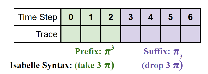
Figure 1: Prefix and suffix notation for traces.

Trace $\pi$ satisfies MLTL formula $\phi$ iff $\pi\models\phi$, where the satisfaction relation $\models$ is defined inductively as follows [18]:

$\pi\models p$ iff $p\in\pi[0]$	$\pi\models\neg\phi$ iff $\pi\not\models\phi$
$\pi\models\phi\wedge\psi$ iff $\pi\models\phi$ and $\pi\models\psi$
$\pi\models\phi\vee\psi$ iff $\pi\models\phi$ or $\pi\models\psi$
$\pi\models\texttt{F}_{[a,b]}\ \phi\text{ iff }|\pi|>a\text{ and }\exists i\in[a,b]\text{ such that }\pi_{i}\models\phi$
$\pi\models\texttt{G}_{[a,b]}\ \phi\text{ iff }|\pi|\leq a\text{ or }\forall i\in[a,b]\ \pi_{i}\models\phi$
$\pi\models\phi\ \texttt{U}_{[a,b]}\ \psi\text{ iff }|\pi|>a\text{ and }\exists i\in[a,b]\text{ such that }\pi_{i}\models\psi$
$\text{ and }\forall j\in[a,i-1]\ \pi_{j}\models\phi$
$\pi\models\phi\ \texttt{R}_{[a,b]}\ \psi\text{ iff }|\pi|\leq a\text{ or }(\forall i\in[a,b]\ \pi_{i}\models\psi)\text{ or }$
$(\exists j\in[a,b]\text{ such that }\pi_{j}\models\phi\text{ and }\forall k\in[a,j]\ \pi_{k}\models\psi$)

The temporal operators $\texttt{F},\texttt{G},\texttt{U},\texttt{R}$ are commonly referred to as “Future,” (see, e.g., [49, 68, 59]) “Globally,” “Until,” and “Release,” respectively. MLTL is modeled off of Linear Temporal Logic (LTL) [52]; like LTL, there is also the option of including more temporal operators in the syntax of MLTL, such as a Next operator and variations on Until and Release, which are easily defined in terms of the above grammar. We design our syntax with a view towards formalizing some current MLTL algorithms, particularly the formula progression algorithm [32] and the MLTL-to-regular expressions algorithm [18], which are defined on the above grammar. However, in any development that necessitates frequent use of additional temporal operators, it would be straightforward to expand our core syntax either by directly creating an alternative expanded version of the syntax or by defining abbreviations for these additional temporal operators. We present our syntactical encoding of MLTL in Sect. 2.1.

We follow the mathematical presentation of MLTL in our formalization; in particular, we define each of the temporal operators $\texttt{F},\texttt{G},\texttt{U},\texttt{R}$ and then formalize important properties of these operators. For this, we mostly follow existing pencil-and-paper proofs [18], deviating as necessary to make the proofs work in Isabelle/HOL. Sect. 2.2 overviews our formalization of MLTL semantics, and Sect. 2.3, Sect. 2.4 present our formalization of basic properties and useful functions for MLTL, respectively.

Although our development is standalone in that it does not import anything other than the standard HOL library, we drew some inspiration from the formalization of a related logic, Linear Temporal Logic (LTL), in Isabelle/HOL [65].

2.1 Syntax

Our syntactic encoding captures the standard formula shapes. For atomic formulas, we allow True (in True_mltl), False (False_mltl), and atomic propositions (Prop_mltl) that take a variable with arbitrary type as an argument (’a is Isabelle’s arbitrary type); we use the arbitrary type to provide maximum flexibility to users of our framework. We allow the usual logical connectives: $\lnot$ (Not_mltl), $\land$ (And_mltl), and $\lor$ (Or_mltl). Lastly, we allow a standard set of temporal operators: future (Future_mltl), globally (Global_mltl), until (Until_mltl), and release (Release_mltl); each temporal operator takes two natural numbers to specify their associated time bounds. Putting it all together, we have the following datatype in Isabelle/HOL to represent MLTL formulas:

datatype (atoms_mltl: ’a) mltl =

    True_mltl | False_mltl | Prop_mltl ’a 

  | Not_mltl "’a mltl" | And_mltl "’a mltl" "’a mltl" 

  | Or_mltl "’a mltl" "’a mltl"            

  | Future_mltl "’a mltl" "nat" "nat" 

  | Global_mltl "’a mltl" "nat" "nat"       

  | Until_mltl "’a mltl" "’a mltl" "nat" "nat"       

  | Release_mltl "’a mltl" "’a mltl" "nat" "nat"

Note that our syntax does not include the standard well-definedness assumption on intervals for temporal operators. For instance, our syntax allows the formula “Future_mltl True_mltl 5 3”, even though this is not a well-defined formula in MLTL. We get around this by explicitly requiring that these intervals have well-defined bounds in our semantics and also by adding this as an assumption in our correctness theorems when necessary.

2.2 Semantics

Because traces are always finite in MLTL, we encode traces as lists of sets of variables of arbitrary type (in Isabelle/HOL, this is type ’a set list). Fig. 2 illustrates our representation of traces in Isabelle/HOL with an example.

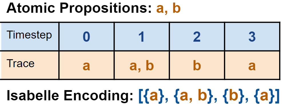
Figure 2: Here, we have two Boolean variables, $a$ and $b$, and four timesteps. At time $0$, variable $a$ is true (and $b$ is false), at time $1$, both $a$ and $b$ are true, and so on. In Isabelle, we would represent this trace as the list $[\{a\},\{a,b\},\{b\},\{a\}]$.

We define the semantics of MLTL formulas in Isabelle/HOL in the function semantics_mltl, which takes a trace $\pi$ and an MLTL formula $\phi$ and returns true if $\pi\models\phi$ and false otherwise. Our formal definition mirrors the mathematical definition, but occasionally makes explicit assumptions that are typically implicit. For example, in the semantics of atomic propositions, we explicitly ensure that if $\emph{$\pi$}\models\emph{\small Prop\_mltl\ p}$ holds, then $\pi$ is nonempty (for well-definedness). Additionally, in the semantics of temporal operators, we explicitly ensure that the associated time bounds are well-defined (i.e, a $\leq$ b).

We now present our formal semantics for a representative subset of operators (Prop_mltl, And_mltl, Global_mltl, and Until_mltl); the full semantics is in Appendix A.1.

fun semantics_mltl::"[’a set list, ’a mltl] $\Rightarrow$ bool"

  where

| "semantics_mltl $\pi$ (Prop_mltl q) = 

     ($\pi$ $\not=$ [] $\wedge$ q $\in$ ($\pi$ ! 0))"

| "semantics_mltl $\pi$ (And_mltl $\varphi$ $\psi$) = 

     (semantics_mltl $\pi$ $\varphi$ $\wedge$ semantics_mltl $\pi$ $\psi$)"

| "semantics_mltl $\pi$ (Global_mltl $\varphi$ a b) = 

     (a $\leq$ b $\wedge$ (length $\pi$$\leq$a $\vee$ ($\forall\,$i::nat. (i$\geq$a $\wedge$ i$\leq$b) 

     $\longrightarrow$ semantics_mltl (drop i $\pi$) $\varphi$)))"

| "semantics_mltl $\pi$ (Until_mltl $\varphi$ $\psi$ a b) = 

     (a$\leq$b $\wedge$ length $\pi$>a $\wedge$ ($\exists\,$i::nat. (i$\geq$a $\wedge$ i$\leq$b) $\wedge$ 

     (semantics_mltl (drop i $\pi$) $\psi$ $\wedge$ ($\forall\,$j. j$\geq$a $\wedge$ j<i 

     $\longrightarrow$ semantics_mltl (drop j $\pi$) $\varphi$))))"

The semantics for Prop_mltl checks that the atomic proposition q is in the set of atomic propositions at the initial timestep (in Isabelle/HOL, this is $\pi$ ! 0, as ! is the operator to access an element from a list), while the semantics for And_mltl checks that trace $\pi$ satisfies both subformulas $\varphi$, $\psi$.

The semantics for Global_mltl checks that the subformula $\varphi$ is satisfied at every step in the trace. More precisely, (Global_mltl $\varphi$ a b) holds automatically if the length of $\varphi$ is less than a; otherwise, for all i between a and b, we must have (drop i $\pi$) $\models$ $\varphi$. Here, (drop i $\pi$) encodes $\pi_{i}$, the suffix of the trace starting at timestep $i$, as drop is Isabelle/HOL’s operator to drop the first $i$ elements from a (zero-indexed) list. Note that our definition for the semantics of Global_mltl includes a well-definedness check to ensure that a$\leq$b.

In other words, the semantics for Until_mltl checks that the subformula $\psi$ is satisfied at some point in the future, and that the subformula $\phi$ is satisfied at every timestep up to that point. We again check a$\leq$b for well-definedness, and then we check that there exists an i between a and b such that (drop i $\pi$) $\models$ $\psi$, and that $\varphi$ is satisfied at all timesteps up to i, i.e., (drop j $\pi$) $\models$ $\varphi$ for all j between a and i-1.

We highlight that the expressiveness of Isabelle/HOL allows us to state the semantics of MLTL formulas essentially verbatim from the mathematical definition, adding in implicit assumptions (like a$\leq$b in the semantics for the temporal operators) when necessary.

Formalizing the semantics in this way further clarifies the differences between MLTL and closely-related logics. Perhaps the most closely-related is MTL-over-naturals [43], with which MLTL differs in five important ways: the traces are finite, the intervals are finite, the internals are closed and unit-less (generic), signal processing is compartmentalized, and the $U$-semantics obeys the interval. Note that the $U$-semantics of MTL-over-naturals is: $\pi\models\phi\ \texttt{U}_{[a,b]}\psi$ iff $|\pi|>a$ and, $\exists i\in[a,\ b],i<|\pi|$ such that $\pi,i\models\psi$ and $\forall j<i$, it holds that $\pi,j\models\phi$. Bounded LTL and its variants (e.g., [38]) share this divergent $U$-semantics. Note that other variants of MTL, such as Metric Interval Temporal Logic (MITL) [3] treat the temporal operator intervals as continuous (rather than discrete) intervals that may be open-ended over real numbers (not integers), and even prohibit singular time intervals, of the form $[a,a]$. Bounded LTL (BLTL) [28] and $\text{LTL}_{f}$ [21] both reason over finite traces like MLTL, but share syntax with LTL; they have (unspecified) finite bounds on the time domain rather than intervals on each temporal operator and keep the $X$ operator. ($\text{LTL}_{f}$ adds a weak next operator as well.)

Throughout our development, we found it useful to have a definition of semantic equivalence for MLTL formulas, where two formulas are semantically equivalent if and only if they are satisfied by the same set of traces. In Isabelle/HOL, we define this as:

definition semantic_equiv:: "’a mltl $\Rightarrow$ ’a mltl $\Rightarrow$ bool"

  where "semantic_equiv $\varphi$ $\psi$ = (

  if ($\forall\,$$\pi$. (semantics_mltl $\pi$ $\varphi$)=(semantics_mltl $\pi$ $\psi$))

  then True else False )"

This function, $\mathtt{semantic\_equiv}$, tests if $\varphi$ and $\psi$ are equivalent by checking if their semantics match on all traces $\pi$.

2.3 Properties

To further establish the correctness of our definitions, and to establish their future usability, we formally prove various essential properties of our encoding of MLTL. Our aim is to establish a reusable formalized library of MLTL properties; this library is useful for both developing future verified tools and algorithms based on MLTL, and as a reference point for theoretical developments involving MLTL.

We first consider properties involving relationships and equivalences between operators. Whereas we explicitly define each core temporal operator (Future, Globally, Until, Release) in terms of its mathematical definition, an alternative approach is to formally define all operators in terms of a functionally complete set of operators for MLTL, like $\{\neg,\land,\texttt{U}\}$ [32], and then derive the typical mathematical definitions for the other operators. This approach is common in the literature [32, 59, 24], and is a primarily stylistic difference. For organizational purposes, we prefer to have all of the mathematical definitions in one place and all of the properties in a separate file. To ensure that our encoding matches the alternative approach, we state and prove key equivalences between operators.

Many of the following equivalences prove easily with Isabelle/HOL’s built-in automation tactics. For example, we establish that Future can be rewritten with Until in the lemma future_as_until by showing that $\texttt{F}_{[a,b]}\phi$ is equivalent to $\text{True}\ \texttt{U}_{[a,b]}\phi$, and we establish the duality of Future and Globally (i.e., that $\texttt{G}_{[a,b]}\phi$ is equivalent to $\neg\texttt{F}_{[a,b]}\neg\phi$) in globally_future_dual. In Isabelle/HOL, we have:

lemma future_as_until:

  fixes a b::"nat"

  assumes "a $\leq$ b"

  shows "semantic_equiv (Future_mltl $\varphi$ a b) 

         (Until_mltl (True_mltl) $\varphi$ a b)"

lemma globally_future_dual:

  fixes a b::"nat"

  assumes "a $\leq$ b"

  shows "semantic_equiv (Global_mltl $\varphi$ a b)

         (Not_mltl (Future_mltl (Not_mltl $\varphi$) a b))"

These two lemmas, alongside DeMorgan’s Laws for $\land$ and $\lor$, are almost enough to establish that $\{\lnot,\land,U\}$ is functionally complete for MLTL. We also need to prove the duality of U and R, i.e., that $\phi\ \texttt{R}_{[a,b]}\psi$ is equivalent to $\neg(\neg\phi\ \texttt{U}_{[a,b]}\neg\psi)$. In Isabelle, we state this in the release_until_dual lemma:

lemma release_until_dual: 

fixes a b::"nat"

assumes a_leq_b: "a $\leq$ b"

shows "semantic_equiv (Release_mltl $\varphi$ $\psi$ a b) 

(Not_mltl (Until_mltl (Not_mltl $\varphi$) (Not_mltl $\psi$) a b))"

This proof does not follow immediately with Isabelle’s automation and was more involved. We follow a proof sketch from the literature [18]. The biconditional statement is split into two implications, and in each direction, the proof considers three cases: ① when the length of the trace is less than $a$, ② when $\psi$ is satisfied for all timesteps in the interval $[a,b]$, and ③ when $\psi$ is not satisfied for some timestep in the interval $[a,b]$. We follow the source material [18] in all cases except for the forward direction of ③; here, we find an error in the source material, which incorrectly reduces a subgoal of showing that $\forall s\in[a,b].(\pi_{s}\models\psi\lor(\exists t\in[a,s-1].\ \pi_{t}\models\phi))$ to showing that $\forall s\in[a,b].(\exists t\in[a,s-1].\ \pi_{t}\models\phi)$. Instead, we directly prove the subgoal with Sledgehammer [45], and then the rest of the proof closed with definition unrolling.

These lemmas are sufficient to establish that any MLTL formula can be rewritten using only the operators $\{\neg,\land,\texttt{U}\}$, which is defined in the literature [32] as the Backus Naur Form (BNF) for MLTL. We verify a custom induction rule, bnf_induct, which allows us to perform structural induction on MLTL formulas in BNF; in Isabelle/HOL, this is:

lemma bnf_induct[case_names IntervalsWellDef PProp 

                 True False Prop Not And Until]:

assumes IntervalsWellDef: "intervals_welldef $\eta$"

and PProp: "($\bigwedge$ $\eta$ $\varphi$. (semantic_equiv $\eta$ $\varphi$ $\longrightarrow$ $\mathcal{P}$ $\eta$ = $\mathcal{P}$ $\varphi$))"

and True: "$\mathcal{P}$ True_mltl"

and False: "$\mathcal{P}$ False_mltl"

and Prop: "$\bigwedge$ p. $\mathcal{P}$ (Prop_mltl p)"

and Not: "$\bigwedge$ $\eta$ $\varphi$. $\mathopen{[\mkern-3.0mu[}$$\eta$ = Not_mltl $\varphi$; $\mathcal{P}$ $\varphi$$\mathclose{]\mkern-3.0mu]}$ $\Longrightarrow$ $\mathcal{P}$ $\eta$"

and And: "$\bigwedge$$\eta$ $\varphi$ $\psi$.  $\mathopen{[\mkern-3.0mu[}$$\eta$ = And_mltl $\varphi$ $\psi$;

    $\mathcal{P}$ $\varphi$; $\mathcal{P}$ $\psi$$\mathclose{]\mkern-3.0mu]}$ $\Longrightarrow$ $\mathcal{P}$ $\eta$"

and Until:"$\bigwedge$$\eta$ $\varphi$ $\psi$ a b.  

    $\mathopen{[\mkern-3.0mu[}$$\eta$ = Until_mltl $\varphi$ $\psi$ a b; $\mathcal{P}$ $\varphi$; $\mathcal{P}$ $\psi$$\mathclose{]\mkern-3.0mu]}$ $\Longrightarrow$ $\mathcal{P}$ $\eta$"

shows "$\mathcal{P}$ $\eta$"

In order to apply this induction rule, we have to prove the IntervalsWellDef and PProp properties. IntervalsWellDef makes explicit an assumption that is typically left implicit: If the MLTL formula $\eta$ that we are trying to perform structural induction on contains any temporal operators, then their corresponding time intervals should be well-defined (for example, if $\eta$ is “Until_mltl a b True_mltl False_mltl”, then a must be less than or equal to b); we formalize this in our intervals_welldef function. PProp stipulates that the property $\mathcal{P}$ that we are trying to prove about MLTL formulas is invariant on semantically equivalent formulas: i.e., for any semantically equivalent formulas $\eta$ and $\varphi$, $\mathcal{P}$ holds on $\eta$ (denoted $\mathcal{P}$ $\eta$) if and only if $\mathcal{P}$ holds on $\varphi$.

Given both IntervalsWellDef and PProp, the induction rule allows us to conclude $\mathcal{P}$ $\eta$ if we can prove property $\mathcal{P}$ on MLTL formulas of the shapes $\eta$ = True_mltl, $\eta$ = False_mltl, and $\eta$ = Prop_mlt p (these are the base cases of the induction rule), and prove the property $\mathcal{P}$ holds on formulas of the shapes $\eta$ = Not_mltl $\varphi$, $\eta$ = And_mltl $\varphi$ $\psi$, and $\eta$ = Until_mltl $\varphi$ $\psi$, given the appropriate inductive hypotheses for each case. When it applies, then, this induction rule is impactful as it considerably reduces the number of cases when compared to the default structural induction proof rule for MLTL formulas (which splits into cases on each operator in our syntax).

We do not limit ourselves to establishing the standard functional completeness for MLTL, but prove a number of additional useful basic properties, like distributivity properties for the Until and Release operators over the logical connectives $\land$ and $\lor$. Most of these prove easily with Isabelle’s built-in automation tactics.

2.4 Useful Functions and Custom Induction Rules

We further flesh out our encodings of the standard MLTL definitions and equivalences to create a reusable library of useful functions on MLTL formulas. Our first useful function is called convert_nnf; it converts an MLTL formula to its negation normal form (NNF), i.e., a logically equivalent formula where negations are only in front of atomic propositions. This function successively applies the operator duality properties to push negations down to the level of atomic propositions. We prove that converting a formula to NNF preserves the semantics of the formula, and also that convert_nnf is idempotent in the following Isabelle/HOL lemmas:

lemma convert_nnf_preserves_semantics:

  assumes "intervals_welldef $\varphi$"

  shows "semantic_equiv $\varphi$ (convert_nnf $\varphi$)"

lemma convert_nnf_convert_nnf:

  shows "convert_nnf (convert_nnf $\varphi$) = convert_nnf $\varphi$"

The proofs of these two lemmas work by induction on the depth of the formula; accordingly, we formalize a depth function for MLTL formulas called depth_mltl. We also define a function called nnf_subformulas to compute the set of subformulas of an MLTL formula, and prove (again by induction on the depth of the formula) that any subformula of a formula in NNF is also in NNF.

lemma nnf_subformulas:

  assumes "$\varphi$ = convert_nnf init_$\varphi$"

  assumes "$\psi$ $\in$ subformulas $\varphi$"

  shows "$\exists\,$ init_$\psi$. $\psi$ = convert_nnf init_$\psi$"

Using these functions and properties, we establish the following custom induction rule, called nnf_induct, as another useful tool for proving properties about MLTL formulas. While the bnf_induct rule reduces the number of cases to consider when proving properties about MLTL formulas, the nnf_induct rule allows us to consider simpler cases when proving properties about MLTL formulas in NNF. In particular, this induction rule requires the property $\mathcal{P}$ to hold on formulas of the each of the standard shapes (True, False, Prop, And, Or, Future, Globally, Until, Release), but limits the Not case to only consider negations of atomic propositions (in case Not_Prop). This induction rule imposes no additional requirements on the property $\mathcal{P}$ (as opposed to the bnf_induct rule, which requires $\mathcal{P}$ to be invariant on semantically equivalent formulas), but does impose the restriction that our input formula $\eta$ is in NNF form (in assumption nnf). Fortunately, all MLTL formulas can be efficiently converted to NNF [18], so this assumption can often be easily satisfied.

lemma nnf_induct[case_names nnf 

                 True False Prop And Or Final 

                 Global Until Release NotProp]:

assumes nnf: "$\exists\,$$\varphi$. $\eta$ = convert_nnf $\varphi$"

and True: "$\mathcal{P}$ True_mltl"

and False: "$\mathcal{P}$ False_mltl"

and Prop: "$\bigwedge$ p. $\mathcal{P}$ (Prop_mltl p)"

and And: "$\bigwedge$$\eta$ $\varphi$ $\psi$.  

    $\mathopen{[\mkern-3.0mu[}$$\eta$ = And_mltl $\varphi$ $\psi$; $\mathcal{P}$ $\varphi$; $\mathcal{P}$ $\psi$$\mathclose{]\mkern-3.0mu]}$ $\Longrightarrow$ $\mathcal{P}$ $\eta$"

and Or: "$\bigwedge$$\eta$ $\varphi$ $\psi$.  

    $\mathopen{[\mkern-3.0mu[}$$\eta$ = Or_mltl $\varphi$ $\psi$;$\mathcal{P}$ $\varphi$; $\mathcal{P}$ $\psi$$\mathclose{]\mkern-3.0mu]}$ $\Longrightarrow$ $\mathcal{P}$ $\eta$"

and Final: "$\bigwedge$$\eta$ $\varphi$  a b.  

    $\mathopen{[\mkern-3.0mu[}$$\eta$ = Future_mltl $\varphi$ a b; $\mathcal{P}$ $\varphi$$\mathclose{]\mkern-3.0mu]}$ $\Longrightarrow$ $\mathcal{P}$ $\eta$"

and Global: "$\bigwedge$$\eta$ $\varphi$  a b. 

    $\mathopen{[\mkern-3.0mu[}$$\eta$ = Global_mltl $\varphi$ a b; $\mathcal{P}$ $\varphi$$\mathclose{]\mkern-3.0mu]}$ $\Longrightarrow$ $\mathcal{P}$ $\eta$"

and Until: "$\bigwedge$$\eta$ $\varphi$ $\psi$  a b. 

    $\mathopen{[\mkern-3.0mu[}$$\eta$ = Until_mltl $\varphi$ $\psi$ a b; $\mathcal{P}$ $\varphi$; $\mathcal{P}$ $\psi$$\mathclose{]\mkern-3.0mu]}$ $\Longrightarrow$ $\mathcal{P}$ $\eta$"

and Release: "$\bigwedge$$\eta$ $\varphi$ $\psi$ a b.  

    $\mathopen{[\mkern-3.0mu[}$$\eta$ = Release_mltl $\varphi$ $\psi$ a b; $\mathcal{P}$ $\varphi$; $\mathcal{P}$ $\psi$$\mathclose{]\mkern-3.0mu]}$ $\Longrightarrow$ $\mathcal{P}$ $\eta$"

and Not_Prop: "$\bigwedge$ $\eta$ p. $\eta$ = 

    Not_mltl (Prop_mltl p) $\Longrightarrow$ $\mathcal{P}$ $\eta$"

shows "$\mathcal{P}$ $\eta$"

Finally, we formalize the computation length of an MLTL formula. The computation length, complen, of an MLTL formula is recursively defined as follows, where $p\in\texttt{AP}$ is a atomic proposition, and $\phi$ and $\psi$ are MLTL formulas [18]:

$$\texttt{complen}(p)=\texttt{complen}(\neg p)=1,$$

$$\texttt{complen}(\phi\land\psi)=\texttt{complen}(\phi\lor\psi)=$$

$$\hskip 40.00006pt\max(\texttt{complen}(\phi),\texttt{complen}(\psi)),$$

$$\texttt{complen}(\texttt{G}_{[a,b]}\phi)=\texttt{complen}(\texttt{F}_{[a,b]}\phi)=b+\texttt{complen}(\phi),$$

$$\texttt{complen}(\phi\ \texttt{U}_{[a,b]}\ \psi)=\texttt{complen}(\phi\ \texttt{R}_{[a,b]}\ \psi)=$$

$$\hskip 40.00006ptb+\max(\texttt{complen}(\phi)-1,\texttt{complen}(\psi))$$

In Isabelle/HOL, we define the complen_mltl function, which maps an MLTL formula of arbitrary type to a natural number, to capture this notion. The definition is essentially verbatim, modulo the requisite syntax changes, except that we add the definition for computation length of True_mltl and False_mltl (both are equal to 1), which were missing from the literature [18]. We present a few representative cases of the formal definition here; the full formal definition is in Appendix A.

fun complen_mltl:: "’a mltl $\Rightarrow$ nat"

where "complen_mltl (Prop_mltl p) = 1"

| "complen_mltl (And_mltl $\varphi$ $\psi$) = 

   max (complen_mltl $\varphi$) (complen_mltl $\psi$)"

| "complen_mltl (Global_mltl $\varphi$ a b) = 

   b + (complen_mltl $\varphi$)"

| "complen_mltl (Until_mltl $\varphi$ $\psi$ a b) = 

   b + (max ((complen_mltl $\varphi$)-1) (complen_mltl $\psi$))"

Computation length is a slightly optimized version of an earlier and closely-related notion of the worst-case propagation delay (wpd) of a formula. Worst-case propagation delay was introduced in the context of runtime verification [29, Definition 5] and was designed to give the maximum number of timesteps an observer needs to wait from the current timestep to decide satisfaction of an MLTL formula so that the decision will not change with further information. For example, if we try to evaluate the satisfaction of $\texttt{F}_{[0,2]}p$ on a trace of length 2, then it is possible that further information could change the verdict. Specifically, $\texttt{F}_{[0,2]}p$ is false on the trace $[\{\},\{\}]$ but true on the trace $[\{\},\{\},\{p\}]$. However, after complen $(\texttt{F}_{[0,2]}p)=3$ timesteps, the value of $p$ in subsequent timesteps will not change whether the trace satisfies $\texttt{F}_{[0,2]}p$. In particular, the R2U2 tool [29], which checks satisfaction of MLTL formulas on traces, does not return an answer until it is certain that the answer will not change with further information. In the worst case, the duration of this delay from the current time is captured by the wpd of the formula.

Interestingly, we found that the computation length also plays a key role in the formal proofs of the formula progression algorithm. Although the source material which we were following [31] does not use or mention computation length, we found that this notion directly fixes some issues with the proofs. We now turn to our formalization of formula progression; we will further discuss computation length and some useful properties we formalize thereof in Sect. 3.4.

3 Formula Progression

Formula progression is a common technique that steps through time to evaluate formulas; it dates back to the 1990’s [7] and has been developed for various temporal logics including MTL [17], $\text{LTL}_{f}$ [41], and MLTL [31]. Formula progression represents a straightforward and generally easy-to-implement algorithm for evaluating whether a particular temporal trace satisfies the given formula, and is therefore utilized in many contexts, including satisfiability solving, validation, runtime verification, and benchmark generation.

Armed with our encoding of MLTL, we discuss our formalization of the MLTL formula progression algorithm and the associated correctness theorems [31]. While we mostly follow the original paper [31] that developed formula progression for MLTL, we found and fixed several errors in the top-level correctness results. In particular, the source material states three key theorems (and a corollary); Fig. 3 overviews these top-level results and our changes to them. We now discuss the formula progression algorithms and each top-level result in turn, with an emphasis on our modifications.

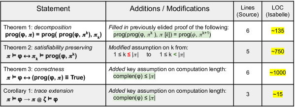
Figure 3: We summarize the top-level results for formula progression and our modifications thereof and compare the number of lines in the proof sketches in the source material [31] with the corresponding LOC in Isabelle/HOL. As our formal proof of Theorem 3 required identifying and formalizing many properties of the computation length, we count these in the LOC.

3.1 Encoding the Formula Progression Algorithm

Formula progression takes an MLTL formula and steps through a trace, partially evaluating the formula at each state in the trace. At each timestep, formula progression partially evaluates the input formula and transforms it into a simplified formula which, under some generally unrestrictive conditions, is logically equivalent. Because MLTL is an inherently bounded logic, it is well-suited for formula progression; one can easily predetermine the number of timesteps needed to transform the input formula into True or False.

The definitions for MLTL formula progression [31, Definition 1] reflect this compatibility, and they are straightforward to formalize. For a trace $\pi$ of length greater than 1, $\text{prog}(\emph{$\varphi$},\emph{$\pi$})$ is defined as $\text{prog}(\text{prog}(\emph{$\varphi$},\emph{$\pi$}[0]),$ $\emph{$\varphi$}_{1})$, which we formalize as the function formula_progression:

fun formula_progression:: 

"’a mltl $\Rightarrow$ ’a set list $\Rightarrow$ ’a mltl" 

where "formula_progression $\varphi$ $\pi$ = 

  (if length $\pi$ = 0 then $\varphi$ 

  else (if length $\pi$ = 1 then 

    (formula_progression_len1 $\varphi$ ($\pi$!0))

  else (formula_progression 

    (formula_progression_len1 $\varphi$ ($\pi$!0)) (drop 1 $\pi$))))"

This function takes an MLTL formula with atoms of arbitrary type and a trace (a list of sets containing elements of the same arbitrary type). To evaluate $\text{prog}(\emph{\small F},\emph{$\pi$}[0])$, it cases on the length of $\pi$. If $\pi$ is empty, it returns F; if $\pi$ has length 1, it calls the helper function formula_progression_len1, which handles formula progression on traces of length 1. When $\pi$ has length longer than 1, it evaluates $\text{prog}(\emph{\small F},\emph{$\pi$}[0])$ as formula_progression_len1 F ($\pi$!0)—here, $\pi$!0 accesses the element at index 0 from $\pi$—and then passes the result to formula_progression on drop 1 $\pi$, where drop n L is Isabelle’s function to drop the first n elements from list L.

The helper function formula_progression_len1 cases on the structure of the input formula, closely following the associated mathematical definitions [31, Definition 1]. As a representative example, we show one of the most complicated cases, for formulas of the shape $\phi\ U_{[a,b]}\ \psi$. Mathematically,

$$\texttt{prog}(\phi\ U_{[a,b]}\ \psi,\emph{$\pi$})=\left\{\begin{array}[]{ll}\phi\ U_{[a-1,b-1]}\ \psi&\mbox{if }0<a\leq b\\ \texttt{prog}(\psi,\emph{$\pi$})\ \lor\\ (\texttt{prog}(\phi,\emph{$\pi$})\ \land\\ \phi\ U_{[0,b-1]}\ \psi)&\mbox{if }0=a<b\\ \texttt{prog}(\psi,\emph{$\pi$})&\mbox{if }0=a=b.\end{array}\right.$$

This is encoded in Isabelle/HOL as follows:

formula_progression_len1 (Until_mltl $\varphi$ $\psi$ a b)

k = (if (0<a$\wedge$a$\leq$b) then (Until_mltl $\varphi$ $\psi$ (a-1) (b-1))

    else (if (0=a$\wedge$a<b) then 

    (Or_mltl (formula_progression_len1 $\psi$ k) 

      (And_mltl (formula_progression_len1 $\varphi$ k) 

      (Until_mltl $\varphi$ $\psi$ 0 (b-1))))

      else (formula_progression_len1 $\psi$ k)))

Aside from notational differences, the only difference between this formal function and the mathematical definition is a minor technical one: the type of formula_progression_len1 is ’a mltl $\Rightarrow$’a set $\Rightarrow$’a mltl, where we use ’a set for the second argument instead of ’a set list because we are (for convenience) directly passing in the singleton element in our trace $\pi$ of length one, which we call k = $\pi$!0. We provide the full formalized function formula_progression_len1 in Appendix B.

We demonstrate the executability of our formalized functions by utilizing Isabelle’s code generation feature to evaluate the formula progression of the formula $\texttt{G}_{[0,2]}p$ on the trace $[\{p\},\{p\},\{\}]$. We visualize the computations involved in this example in Figure 4; here, we are using the value command in Isabelle/HOL (which invokes the code generator [23]) to evaluate intermediate steps of the formula progression algorithm. It is important to note that the formula progression algorithm is not guaranteed to produce an output in the simplest form; our verified implementation produces a final output of $\neg((\neg\text{True})\lor((\neg\text{True})\lor(\neg\text{False})))$, which is logically equivalent to False.

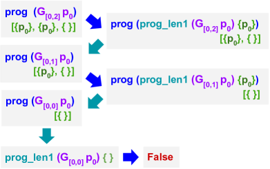
Figure 4: We illustrate the recursive calls that the formula progression algorithm makes to transform the formula $G_{[0,2]}p$ on the trace $[\{p\},\{p\},\{\}]$ to the formula False. The formula requires that $p$ is true at every timestep from $0$ to $2$; in timesteps $0$ and $1$, $p$ is true, and thus the time bound is reduced from $[0,2]$ to $[0,1]$ and then to $[0,0]$. In the final timestep, $p$ is false (since the state is empty and does not contain $p$), and so formula progression ultimately returns False. Note that the output of formula progression is not guaranteed to be in the simplest form; in this example, our verified implementation produces $\neg((\neg\text{True})\lor((\neg\text{True})\lor(\neg\text{False})))$, which is logically equivalent to False.

3.2 Verifying Theorem 1

The first key theorem for formula progression informally states that performing formula progression along a trace can be split into first performing formula progression on the prefix, and then on the suffix, of that trace. Mathematically, it states that $\texttt{prog}(\phi,\pi)=\texttt{prog}(\texttt{prog}(\phi,\pi^{k}),\pi_{k})$ for $1\leq k\leq\texttt{length }\pi$. In Isabelle, we prove the following theorem, formula_progression_decomposition, where “take k $\pi$” is the function to take the first $k$ elements of the list $\pi$ (lists are zero-indexed, so this is the prefix of $\pi$ from $0$ to $\emph{\small k}-1$, which is $\pi^{k}$) and “drop k $\pi$” is the function to drop the first $k$ elements of the list $\pi$ (which is $\pi_{k}$; cross-reference Fig. 1).

theorem formula_progression_decomposition:

  fixes $\varphi$::"’a mltl"

  assumes "k $\geq$ 1"

  assumes "k $\leq$ length $\pi$"

  shows "formula_progression 

    (formula_progression $\varphi$ (take k $\pi$)) (drop k $\pi$)

    = formula_progression $\varphi$ $\pi$"

Our formal proof of this theorem follows the proof sketch in the original source paper [31] relatively closely.

We found it effective to split out the following identity used in the proof into a separate helper lemma:
$\text{prog}(\text{prog}(\phi,\pi^{k}),\pi[k])=\text{prog}(\phi,\pi^{k+1})$.

Although the source paper stated that this property holds by definition, we proceeded to prove this by a more involved induction on $k$. This highlights the role of formalization, which necessitates making all handwaving in source proofs rigorous. Even so, Theorem 1 was the easiest of the three top-level formula progression theorems to prove, and its proof only required about 135 LOC (compared to 6 lines of proof in the source material).

3.3 Verifying Theorem 2

The second key theorem for formula progression states that (in most cases) the formula progression of a formula on a trace is logically equivalent to the formula progression of the prefix of the trace on its suffix. Mathematically, this is $\pi\models\phi$ iff $\pi_{k}\models\text{prog}(\phi,\pi^{k})$; the source material [31] stated this theorem for $1\leq k\leq\text{length }\pi$, but our formal statement is for $1\leq k<\text{length }\pi$. In Isabelle/HOL, we have:

theorem satisfiability_preservation:

  fixes $\varphi$::"’a mltl"

  assumes "k $\geq$ 1"

  assumes "k < length $\pi$"

  assumes "intervals_welldef $\varphi$"

  shows "semantics_mltl (drop k $\pi$) 

      (formula_progression $\varphi$ (take k $\pi$)) 

      $\longleftrightarrow$ semantics_mltl $\pi$ $\varphi$"

In addition to altering the bound on k, we also add a well-definedness assumption (intervals_welldef $\varphi$) which asserts that all temporal operators have well-defined timebounds (e.g., if $\varphi$ is $\emph{\small Release\_mltl}\ \emph{$\psi$}\ \emph{$\eta$}\ a\ b$, then $a\leq b$). This well-definedness assumption is typically included as part of the MLTL syntax; it is an artifact of formalization that our syntax does not enforce this well-definedness and it must be made explicit here (cross-reference Sect. 2.1).

The altered bound, however, is mathematically necessary for the correctness of the result and was overlooked in the source material. We uncovered this while formalizing the base case of this theorem. The source material inducts on $k$ and states that the base case (where $k=1$) is by induction without providing details; which caused issues when working in Isabelle/HOL. The issue we run into here is related to end-of-trace behavior. When both $k=1$ and the length of $\pi$ is 1, the statement of Theorem 2 becomes $\pi\models\phi\longleftrightarrow[]\models\texttt{prog}(\phi,\pi)$, and this does not hold in general.

Specifically, consider a formula of the shape $\texttt{G}_{[0,b]}p$ for $b>0$ with trace $\pi=[\{p\}]$ of length $1$. If we allow $k=1$, then we would want to establish $\pi\models\texttt{G}_{[0,b]}p\longleftrightarrow\pi_{1}\models\texttt{prog}(\texttt{G}_{[0,b]}\phi,\pi^{1})$. We have that $\pi_{1}=[]$ and $\pi^{1}=\pi$, so this becomes $\pi\models\texttt{G}_{[0,b]}p\longleftrightarrow[]\models\texttt{prog}(\texttt{G}_{[0,b]}p,\pi)$. Then using the semantics of MLTL on the left-hand side, $\pi\models\texttt{G}_{[0,b]}p$ reduces to $\forall i\in[0,b].\ \pi_{i}\models p$, which further reduces to $\forall i\in[0,b].(\pi_{i}\neq[]\land p\in\pi_{i}[0])$. However, this is false because $\pi_{1}=[]$.

Applying the definition of formula progression to the right-hand side, we have that:

$$\texttt{prog}(\texttt{G}_{[0,b]}p,\pi) =\neg\texttt{prog}(\texttt{F}_{[0,b]}\neg p,\pi)$$

$$=\neg(\neg\texttt{prog}(p,\pi)\lor\texttt{F}_{[0,b-1]}\neg p)$$

$$=\neg(\neg true\lor\texttt{F}_{[0,b-1]}\neg p)$$

$$=\neg\texttt{F}_{[0,b-1]}\neg p$$

$$=\texttt{G}_{[0,b-1]}p\ \text{, Future and Globally are duals}$$

Thus, the right-hand side becomes $[]\models\texttt{G}_{[0,b-1]}p$; using the semantics of MLTL this is $|[]|\leq 0\lor(\forall i\in[0,b-1].\ []_{i}\models p)$, which is true because the left disjunct is true.

Fortunately, modifying the statement of Theorem 2 to insist $k<\text{length}\ \pi$ instead of $k\leq\text{length}\ \pi$ removes this issue (because, for $k=1$, our traces $\pi$ must have length at least 2, so we do not encounter the above issues with the empty trace). Further, and crucially, we are still able to use our modified version of Theorem 2 in the proofs of Theorem 3 and the top-level corollary; that is, our modification fixes Theorem 2 without overly weakening the result.

3.4 Verifying Theorem 3 and Corollary 1

The third key theorem for formula progression informally states that, for a sufficiently long input trace $\pi$, and for a well-defined input formula $\varphi$, $\pi$ models formula $\varphi$ if and only if the formula progression of $\varphi$ over $\pi$ is logically equivalent to True. More precisely, we require (in the first assumption) that all intervals in $\varphi$ are well-defined, and we require (in the second assumption) that the length of $\pi$ is at least the computation length of the formula (cross-reference Sect. 2.4, [18]). In Isabelle, we have the following theorem, where semantic_equiv encodes logical equivalence of two MLTL formulas (cross-reference Sect. 2.4):

theorem formula_progression_correctness:

  fixes $\varphi$::"’a mltl"

  assumes "intervals_welldef $\varphi$"

  assumes "length $\pi$ $\geq$ complen_mltl $\varphi$"

  shows "(semantic_equiv (formula_progression $\varphi$ $\pi$) 

    True_mltl)  $\longleftrightarrow$ semantics_mltl $\pi$ $\varphi$"

While the assumption that all intervals in $\varphi$ are well-defined can again be viewed as something of a formalization curiosity as it is typically mathematically implicit, the assumption that the length of $\pi$ is greater than or equal to the computation length of the formula $\varphi$ is mathematically crucial for the correctness of the theorem. Notably, this assumption was missing in the corresponding theorem in the original source material [31, Theorem 3]; identifying it is a contribution of our formalization. Fortunately, adding in this assumption does not affect the practicality of formula progression; in practice, traces are typically long streams of data, so it is not overly restrictive to assume that a trace is sufficiently long.

We identified this assumption when attempting to prove the base case of Theorem 3. The source material states that this is by structural induction and omitted all mathematical details. When initially attempting to formalize the base case without this critical assumption, we quickly ran into issues in the Or_mltl case. To see why, let us consider the proof on a mathematical level. We are trying to prove that $(\pi\models\phi\lor\psi)\longleftrightarrow(\text{prog}(\phi\lor\psi,\pi)=\text{True})$ for a trace $\pi$ of length 1, given that $(\pi\models\phi)\longleftrightarrow(\text{prog}(\phi,\pi)=\text{True})$ and $(\pi\models\psi)\longleftrightarrow(\text{prog}(\psi,\pi)=\text{True})$. Because $\text{prog}(\phi\lor\psi,\pi)$ is defined as $\text{prog}(\phi,\pi)\lor\text{prog}(\psi,\pi)$ when $\pi$ has length 1, and using that $\pi\models\phi\lor\psi\longleftrightarrow(\pi\models\phi\lor\pi\models\psi)$, our goal becomes $(\pi\models\phi\lor\pi\models\psi)\longleftrightarrow((\text{prog}(\phi,\pi)\lor\text{prog}(\phi,\pi))=\text{True})$. Then, using our inductive hypotheses, we incur the goal: $(\text{prog}(\psi,\pi)=\text{True}\lor\text{prog}(\phi,\pi)=\text{True})\longleftrightarrow((\text{prog}(\phi,\pi)\lor\text{prog}(\psi,\pi))=\text{True})$. This does not hold; $\text{prog}(\phi,\pi)\lor\text{prog}(\psi,\pi)$ can be logically equivalent to True without either $\text{prog}(\phi,\pi)$ or $\text{prog}(\psi,\pi)$ being logically equivalent to True; all that is required is that $\text{prog}(\phi,\pi)$ must hold in any states where $\text{prog}(\psi,\pi)$ is false and vice-versa.

By adding the assumption on the computation length, the base case of the formula progression theorem inherits the (structurally strong) assumption that $1$ is greater than or equal to the computation length of the input formula $\phi$. This assumption is strong enough to establish that the formula progression of $\phi$ on any trace of length 1 is either globally true or globally false. This solves the above issue in the Or_mltl case; since $(\text{prog}(\phi,\pi)$ and $(\text{prog}(\psi,\pi)$ are now globally either True or False, we can indeed conclude $(\text{prog}(\psi,\pi)=\text{True}\lor\text{prog}(\phi,\pi)=\text{True})\longleftrightarrow((\text{prog}(\phi,\pi)\lor\text{prog}(\psi,\pi))=\text{True})$, as desired. We establish this useful property of the computation length in the following key lemma:

lemma complen_bounded_by_1:

  fixes $\pi$::"’a set list"

  assumes "intervals_welldef $\varphi$"

  assumes "1 $\geq$ complen_mltl $\varphi$"

  shows "($\forall\,$$\eta$. semantics_mltl $\eta$

    (formula_progression_len1 $\varphi$ ($\pi$!0)) = True) 

    $\vee$ ($\forall\,$$\eta$. semantics_mltl $\eta$

    (formula_progression_len1 $\varphi$ ($\pi$!0)) = False)"

This lemma is sufficient to prove our strengthened base case; however, we also need to ensure that the strengthened base case is usable in the proof of Theorem 3. This requires adding several additional properties of the computation length. In particular, we establish the following two crucial properties:

lemma complen_one_implies_one:

  assumes "intervals_welldef $\varphi$"

  assumes "complen_mltl $\varphi$ = 1"

  shows "complen_mltl (formula_progression $\varphi$ $\pi$) = 1"

lemma formula_progression_decreases_complen:

  assumes "intervals_welldef $\varphi$"

  shows "complen_mltl $\varphi$ = 1 $\vee$ 

         complen_mltl (formula_progression $\varphi$ $\pi$) = 1 $\vee$ 

         complen_mltl (formula_progression $\varphi$ $\pi$) 

         $\leq$ complen_mltl $\varphi$ - (length $\pi$)"

This first lemma, complen_one_implies_one, proves that (for formulas $\varphi$ with well-defined intervals), if the computation length of $\varphi$ is 1, then the computation length of the formula progression of $\varphi$ is also 1; i.e., formula progression does not increase the computation length for formulas that already have the minimum computation length. The second key lemma, formula_progression_decreases_complen, establishes that performing formula progression on a formula $\varphi$ over a trace $\pi$ usually decreases the computation length of $\varphi$ proportionally to the length of $\pi$. More precisely, either the computation length of $\varphi$ equals 1 (i.e., is already minimal), or the computation length of the formula progression of $\varphi$ on trace $\pi$ equals 1 (i.e., is minimal), or the computation length of the formula progression of $\varphi$ on $\pi$ is less than or equal to the computation length of $\varphi$ minus the length of the trace $\pi$ (i.e., the computation length of the progression is decreased by the length of $\pi$).

We use complen_one_implies_one in the proof of formula _progression_decreases_complen, and we use both of these lemmas in the proof of Theorem 3 to establish that complen $\text{prog}(\phi,(\pi^{\text{length }\pi-1}))\leq\text{length}(\pi_{\text{\ length }\pi-1})$, which is equivalent to complen $\text{prog}(\phi,(\pi^{\text{length }\pi-1}))\leq 1$. This then allows us to use the base case of Theorem 3 with the formula $\text{prog}(\phi,(\pi^{\text{length }\pi-1}))$ and the trace $\pi_{\text{\ length }\pi-1}$ to prove that $\text{prog}(\text{prog}(\phi,(\pi^{\text{length }\pi-1}),\pi_{\text{\ length }\pi-1}))=\text{True}$ is equal to $\pi_{\ \text{length }\pi-1}\models\text{prog}(\phi,(\pi^{\text{length }\pi-1}))$. Then, following the source material [31], we can conclude that ① $\text{prog}(\text{prog}$ $(\phi,(\pi^{\text{length }\pi-1}),\pi_{\text{\ length }\pi-1}))=\text{prog}(\phi,\pi)$ using Theorem 1 and ② $\pi_{\text{\ length }\pi-1}\models$ $\text{prog}(\phi,(\pi^{\text{length }\pi-1}))$ iff $\pi\models\phi$ using Theorem 2. Putting these pieces together closes the proof.

In total, formula_progression_correctness took approximately 1000 lines of code to formalize (this includes about 800 lines for establishing the necessary properties of the computation length), as compared to 6 lines in the original source material.

Putting the three key theorems together, we achieve the following top-level corollary, which informally states that, for a well-defined MLTL formula $\varphi$ and a sufficiently long trace $\pi$, if $\emph{$\pi$}\models\emph{$\varphi$}$, then any trace whose prefix is $\pi$ also models $\varphi$. Formally, we prove the following result in Isabelle/HOL, where @ is Isabelle/HOL’s syntax for appending lists.

corollary trace_append:

  fixes $\varphi$::"’a mltl"

  assumes "intervals_welldef $\varphi$"

  assumes "length $\pi$ $\geq$ complen_mltl $\varphi$"

  assumes "semantics_mltl $\pi$ $\varphi$"

  shows "semantics_mltl ($\pi$ @ $\zeta$) $\varphi$"

The source material [31, Corollary 1] had stated this corollary without the key assumption on the length of the trace, but that is incorrect. To see why, consider the following example. We know that $[\{2\}]\models G_{[1,3]}\text{False}$, as the length of the trace $[\{2\}]$ is $\leq 1$ (cross-reference the mathematical semantics of MLTL presented in Sect. 2). From this, without the assumption that $[\{2\}]$ must be greater than or equal to the computation length of $G_{[1,3]}\text{False}$, which is 4, we could obtain, for example, $[\{2\},\{3\},\{4\},\{2,3\}]\models G_{[1,3]}\text{False}$, which contradicts the semantics of MLTL. Fortunately, after adding in this assumption, the (formal) proof of this corollary is quite straightforward and follows the proof presented in the source material [31] without issue.

After formalizing this corollary, we realized that we could go one step further to also formalize an alternate version of Theorem 3: If a sufficiently long trace $\pi$ does not satisfy a formula $\phi$, then the formula progression of $\phi$ on $\pi$ is logically equivalent to False. Although the proof of this exactly mirrors the proof of Theorem 3, it is not immediately implied by Theorem 3; assuming that $\pi\not\models\phi$, Theorem 3 only yields that the $\text{prog}(\phi,\pi)$ is not semantically equivalent to True. This does not necessitate that the resulting formula is semantically equivalent to False.

Combining the original and alternate versions of Theorem 3, we obtain the following important property of formula progression:

lemma formula_progression_true_or_false:

  fixes $\varphi$::"’a mltl"

  assumes "intervals_welldef $\varphi$"

  assumes "length $\pi$ $\geq$ complen_mltl $\varphi$"

  assumes "$\psi$ = (formula_progression $\varphi$ $\pi$)"

  shows "(semantic_equiv $\psi$ False_mltl)

       $\vee$ (semantic_equiv $\psi$ True_mltl)"

This allows us to conclude that for a sufficiently long trace $\pi$, the formula progression of $\phi$ on $\pi$ is either logically equivalent to True or False. In fact, our earlier result
complen_bounded_by_1 is a special case of this more general property.

We also use our alternate version of Theorem 3 to prove the inverse of the top-level corollary, strengthening it to an if-and-only-if statement:

corollary trace_append_iff:

  fixes $\varphi$::"’a mltl"

  assumes "intervals_welldef $\varphi$"

  assumes "length $\pi$ $\geq$ complen_mltl $\varphi$"

  shows "semantics_mltl $\pi$ $\varphi$ $\longleftrightarrow$ 

        ($\forall\,$$\zeta$. semantics_mltl ($\pi$ @ $\zeta$) $\varphi$)"

This says that for a sufficiently long trace $\pi$, extending $\pi$ with any additional states (in $\zeta$) does not affect the satisfaction of formula $\phi$. This formalizes the intuition for computation length, that timesteps beyond the computation length of a formula do not affect the satisfaction of that formula. Retrospectively, one bonus of our formalization is that it nicely integrates various related concepts (like formula progression and computation length) for MLTL in a single centralized and easily extensible library.

4 Challenges and Insights

We view our formalization as emblematic of the potential benefits of formalizing source material that heavily relies on intuition. The mathematical intuition for formula progression for MLTL is clear because of its boundedness. Accordingly, the original source material heavily leaned into this intuition, and many important details were elided (possibly in light of space constraints), which introduced bugs. In particular, the base cases of Theorem 2 and Theorem 3 claimed to hold by structural induction; mathematically, this seems quite intuitive. However, formalization serves as a useful forcing function, where all intuition must be made precise, and in the course we found that the base cases were incorrect as stated and needed modifications; these then propagated into the top-level theorems and corollary.

One of the main creative challenges that we faced was identifying the necessary assumptions to add to these two base cases. These added assumptions needed to walk a fine line. On the one hand, they must be strong enough to prove the base cases. On the other hand, they must be weak enough that they can still be used to prove the desired top-level result. Additionally, we wanted our additional assumptions to maintain the practicality of formula progression. We found that it was useful to keep the high-level context in mind throughout the course of our formalization; we frequently switched back and forth between working on a base case and using that base case to prove the overall desired result.

Similarly, it was only by analyzing the top-level corollary that we identified the main necessary assumption for Theorem 3 (that length  $\pi$  $\geq$ complen_mltl  $\varphi$). Mathematically, we found it intuitively clear that this assumption would be sufficient to establish the corollary and that it would not affect the practicality of formula progression (because traces in real-world systems tend to be long). Interestingly, though, we were initially unsure whether it was strong enough to fix the formalization of the proof of Theorem 3. Establishing this required identifying and proving various key properties of the computation length, particularly those discussed in Sect. 3, which establish that formula progression tends to decrease computation length. Initially, we stated these in a series of (unproven) properties of the computation length that we wanted to be able to use in our proofs (as a sort of wishlist); we were pleasantly gratified when we later found that all of these necessary properties held.

Another key challenge that we encountered was related to end-of-trace behavior. We noticed this especially in the proof of Theorem 2, where the behavior of the empty trace caused issues in the theorem as it was originally stated. In practice, MLTL traces are typically long, and we suspect this is why it is easy to overlook the edge cases where we are reasoning about the empty trace. Additionally, MLTL end-of-trace behavior is somewhat unintuitive; for example, $[]\models G_{[0,1]}\text{False}$ according to MLTL semantics, because Globally is satisfied if the length of the trace is less than or equal to the lower bound on its associated interval. Fortunately, formalization is excellent at making strange edge cases precise and ensuring that they are correctly reasoned about.

Finally, we wish to comment on our choice of the theorem prover Isabelle/HOL, which we benefited from throughout the formalization. We particularly appreciate the automation afforded by Sledgehammer [45] and also the built-in support for unrolling definitions and functions; the latter was extremely helpful in a number of our proofs that rely on structural induction and reduce into detailed casework. We also appreciate Isabelle’s well-developed libraries; though our work does not depend on any entries from the Archive of Formal Proofs, we loosely modeled our formalization of MLTL syntax and semantics on an existing formalization of LTL [65].

5 Discussion and Future Work

Our work serves to refine and unify the previously-published semantics, algorithms, and definitions for MLTL. In particular, as the crown jewel of our formalization, we verify the formula progression algorithm [31]; along the way, we fix some errors in the correctness proofs. We also develop the foundational notion of computation length [18]. In general, we found that the source material was somewhat piecemeal in its development of this notion of computation length and its counterpart, worst-case propagation delay [29]. One contribution of our formalization is establishing a centralized body of lemmas about the computation length, and it is an exciting area of future work to continue to develop this corpus. We can now work toward establishing that the computation length is minimal, and proving related results from the literature, particularly ones involving worst-case propagation delay, e.g. [69, Lemma 4].

Our formalization of the syntax, semantics, duality properties, an NNF transformation, custom induction rules, and a formula progression algorithm constitutes a useful library that facilitates future formal developments for MLTL and serves as a useful reference point for theoretical developments. In particular, we envision a suite of formally verified algorithms for MLTL that can be used to validate the existing (unverified) tools for analyzing MLTL formulas, or which could be developed into tools in their own right. We ensure the executability of our algorithms and generate a code export so that they can be used to validate existing (unverified) tool support, i.e., the FPROGG tool, which implements formula progression in C [54]. We envision creating a conformance tester for MLTL, similar to the success of VeriMon for related modal logics [8]. In this way, our library can also serve to create provably-correct benchmarks for evalation of MLTL satisfiability and runtime verification. A common reason why competitions like the 2018 attempt to start a Runtime Verification Competition [1] fail is due to a lack of a large, challenging, and correct set of benchmarks. Such formalizations also serve to validate existing tool implementations. For example, the PVS formalization of MTL was created to verify a translation from a structured natural language called FRETish to MTL in order to validate the tool FRET [12]. Now the Isabelle/HOL formalization of MLTL can serve a similar role in validating all of the tools that natively analize MLTL and other logics for which it is a subset.

Since MLTL is a commonly-used subset of other popular logics like STL and MTL, our library also lays a foundation for their future formalization in Isabelle/HOL. In particular, a natural next step would be utilizing our library in a formalization of the syntax, semantics, and related lemmas for MTL-over-naturals. From there, it will be possible to keep building formalizations of other MTL variants, such as the list in [43]. The library we have created here will serve as a necessary component of any future efforts to formalize more complex semantics that extend MLTL, such as STL.

6 Acknowledgements

Thanks to Alec Rosentrater for useful comments and feedback on the paper and to Alexis Aurandt and Brian Kempa for useful discussions about worst-case propagation delay. Thanks to NSF CAREER Award CNS-1552934 and NSF CCRI-2016592 for supporting this work. Zili Wang was supported by an NSF Graduate Research Fellowship under NSF:GRFP 2024364991.

Appendix A Appendix A

In this appendix, we present some of the code snippets for functions that we did not include (or only partially included) in the main body of the paper. These may also be found in our code, but we include them here for easy reference.

A.1 MLTL Semantics

We present our full formal definition of the semantics of MLTL (cross-reference Sect. 2).

fun semantics_mltl::"[’a set list, ’a mltl] $\Rightarrow$ bool"

  where

  "semantics_mltl $\pi$ True_mltl = True"

| "semantics_mltl $\pi$ False_mltl = False"

| "semantics_mltl $\pi$ (Prop_mltl q) = 

     ($\pi$ $\not=$ [] $\wedge$ q $\in$ ($\pi$ ! 0))"

| "semantics_mltl $\pi$ (Not_mltl $\varphi$) = 

     ($\neg$ (semantics_mltl $\pi$ $\varphi$))"

| "semantics_mltl $\pi$ (And_mltl $\varphi$ $\psi$) = 

     (semantics_mltl $\pi$ $\varphi$ $\wedge$ semantics_mltl $\pi$ $\psi$)"

| "semantics_mltl $\pi$ (Or_mltl $\varphi$ $\psi$) = 

     (semantics_mltl $\pi$ $\varphi$ $\vee$ semantics_mltl $\pi$ $\psi$)"

| "semantics_mltl $\pi$ (Future_mltl $\varphi$ a b) = 

     (a$\leq$b $\wedge$ length $\pi$>a $\wedge$ ($\exists\,$i::nat. 

     (i$\geq$a $\wedge$ i$\leq$b) $\wedge$ semantics_mltl (drop i $\pi$) $\varphi$))"

| "semantics_mltl $\pi$ (Global_mltl $\varphi$ a b) = 

     (a $\leq$ b $\wedge$ (length $\pi$$\leq$a $\vee$ ($\forall\,$i::nat. (i$\geq$a $\wedge$ i$\leq$b) 

     $\longrightarrow$ semantics_mltl (drop i $\pi$) $\varphi$)))"

| "semantics_mltl $\pi$ (Until_mltl $\varphi$ $\psi$ a b) = 

     (a$\leq$b $\wedge$ length $\pi$>a $\wedge$ ($\exists\,$i::nat. (i$\geq$a $\wedge$ i$\leq$b) $\wedge$ 

     (semantics_mltl (drop i $\pi$) $\psi$ $\wedge$ ($\forall\,$j. j$\geq$a $\wedge$ j<i 

     $\longrightarrow$ semantics_mltl (drop j $\pi$) $\varphi$))))"

| "semantics_mltl $\pi$ (Release_mltl $\varphi$ $\psi$ a b) = 

   (a$\leq$b $\wedge$ (length $\pi$$\leq$a $\vee$ ($\forall\,$i::nat. (i$\geq$a $\wedge$ i$\leq$b) $\longrightarrow$ 

   (semantics_mltl (drop i $\pi$) $\psi$)) $\vee$ 

   ($\exists\,$j. j$\geq$a $\wedge$ j$\leq$b-1 $\wedge$ semantics_mltl (drop j $\pi$) $\varphi$ 

      $\wedge$ ($\forall\,$k. a$\leq$k $\wedge$ k$\leq$j $\longrightarrow$

      semantics_mltl (drop k $\pi$) $\psi$))))"

This semantics is designed to closely match the mathematical semantics of MLTL while also including the well-definedness assumption for temporal operators (that a $\leq$b).

A.2 Well-Defined Intervals

We present our Isabelle/HOL function intervals_welldef, which checks if all intervals associated to temporal operators in an input formula are well-defined.

fun intervals_welldef:: "’a mltl $\Rightarrow$ bool"

  where "intervals_welldef True_mltl = True"

  | "intervals_welldef False_mltl = True"

  | "intervals_welldef (Prop_mltl p) = True" 

  | "intervals_welldef (Not_mltl $\varphi$) = intervals_welldef $\varphi$"

  | "intervals_welldef (And_mltl $\varphi$ $\psi$) = 

  (intervals_welldef $\varphi$ $\wedge$ intervals_welldef $\psi$)"     

  | "intervals_welldef (Or_mltl $\varphi$ $\psi$) = 

  (intervals_welldef $\varphi$ $\wedge$ intervals_welldef $\psi$)"     

  | "intervals_welldef (Future_mltl $\varphi$ a b)  = 

  (a $\leq$ b $\wedge$ intervals_welldef $\varphi$)"

  | "intervals_welldef (Global_mltl $\varphi$ a b)  = 

  (a $\leq$ b $\wedge$ intervals_welldef $\varphi$)"

  | "intervals_welldef (Until_mltl $\varphi$ $\psi$ a b)  = 

  (a $\leq$ b $\wedge$ intervals_welldef $\varphi$ $\wedge$ intervals_welldef $\psi$)"

  | "intervals_welldef (Release_mltl $\varphi$ $\psi$ a b)  = 

  (a $\leq$ b $\wedge$ intervals_welldef $\varphi$ $\wedge$ intervals_welldef $\psi$)"

This function is recursively defined. It returns True on formulas that clearly have no temporal operators (True_mltl, False_mltl, and Prop_mltl). For formulas of shapes And_mltl, Not_mltl, and Or_mltl, intervals_welldef checks whether the relevant subformulas contain well-defined intervals. For example, for And_mltl $\varphi$ $\psi$, this function checks whether the intervals in $\varphi$ and $\psi$ are well-defined. For the temporal operators, intervals_welldef checks whether the top-level interval is well-defined and also whether the intervals of any relevant subformulas are well-defined. For example, for intervals_welldef Future_mltl $\varphi$ a b to hold, we must have both a $\leq$ b and also intervals_welldef $\varphi$.

A.3 Computation Length

We present our full encoding of the comptuation length of an MLTL formula complen_mltl (cross-reference Sect. 2.4).

fun complen_mltl:: "’a mltl $\Rightarrow$ nat"

where "complen_mltl False_mltl = 1"

| "complen_mltl True_mltl = 1"

| "complen_mltl (Prop_mltl p) = 1"

| "complen_mltl (Not_mltl $\varphi$) = complen_mltl $\varphi$"

| "complen_mltl (And_mltl $\varphi$ $\psi$) = 

   max (complen_mltl $\varphi$) (complen_mltl $\psi$)"

| "complen_mltl (Or_mltl $\varphi$ $\psi$) = 

   max (complen_mltl $\varphi$) (complen_mltl $\psi$)"

| "complen_mltl (Global_mltl $\varphi$ a b) = 

   b + (complen_mltl $\varphi$)"

| "complen_mltl (Future_mltl $\varphi$ a b) = 

   b + (complen_mltl $\varphi$)"

| "complen_mltl (Release_mltl $\varphi$ $\psi$ a b) = 

   b + (max ((complen_mltl $\varphi$)-1) (complen_mltl $\psi$))"

| "complen_mltl (Until_mltl $\varphi$ $\psi$ a b) = 

   b + (max ((complen_mltl $\varphi$)-1) (complen_mltl $\psi$))"

Appendix B Appendix B

We detail the full formula progression function, and we present the correspoding encoding of the corresponding function in Isabelle, formula_progression_len1 (cross-reference Sect. 3.1).

Let $\pi$ be a trace and $\phi$ and $\psi$ be MLTL formulas. The formula progression of $\phi$ on $\pi$, denoted $\texttt{prog}(\phi,\pi)$, is defined recursively as follows [31, Definition 1]:

• If $|\pi|=1$, then

  • $\texttt{prog}(\text{True},\pi)=\text{True}$ and $\texttt{prog}(\text{False},\pi)=\text{False}$;

  • if $\phi=p$ is an atomic proposition,
    $\texttt{prog}(p,\pi)=\text{True}$ if and only if $p\in\pi[0]$;

  • $\texttt{prog}(\neg\phi,\pi)=\neg\texttt{prog}(\phi,\pi)$;

  • $\texttt{prog}(\phi\lor\psi,\pi)=\texttt{prog}(\phi,\pi)\lor\texttt{prog}(\psi,\pi)$;

  • $\texttt{prog}(\phi\land\psi,\pi)=\texttt{prog}(\phi,\pi)\land\texttt{prog}(\psi,\pi)$;

  • $\texttt{prog}(\phi\texttt{U}_{[a,b]}\psi,\pi)=\left\{\begin{array}[]{ll}\phi\ U_{[a-1,b-1]}\ \psi&\mbox{if }0<a\leq b;\\ \texttt{prog}(\psi,\emph{$\pi$})\ \lor\\ (\texttt{prog}(\phi,\emph{$\pi$})\ \land\\ \phi\ U_{[0,b-1]}\ \psi)&\mbox{if }0=a<b;\\ \texttt{prog}(\psi,\emph{$\pi$})&\mbox{if }0=a=b;\end{array}\right.$

  • $\texttt{prog}(\texttt{F}_{[a,b]}\phi,\pi)=\left\{\begin{array}[]{ll}\texttt{F}_{[a-1,b-1]}\phi&\mbox{if }0<a\leq b;\\ \texttt{prog}(\phi,\pi)\lor\\ \texttt{F}_{[0,b-1]}\phi&\mbox{if }0=a<b;\\ \texttt{prog}(\phi,\pi)&\mbox{if }0=a=b;\end{array}\right.$

  • $\texttt{prog}(\phi\texttt{R}_{[a,b]}\psi,\pi)=\neg\texttt{prog}((\neg\phi)\texttt{U}_{[a,b]}(\neg\psi),\pi)$;

  • $\texttt{prog}(\texttt{G}_{[a,b]}\phi,\pi)=\neg\texttt{prog}(\texttt{F}_{[a,b]}(\neg\phi),\pi)$.

• Else, $\texttt{prog}(\phi,\pi)=\texttt{prog}(\texttt{prog}(\phi,\pi[0]),\pi_{1}).$

The $|\pi|>1$ case is described in detail in the Isabelle function formula_progression in Sect. 3.1. We present the full $|\pi|=1$ case as the function formula_progression_len1 in Isabelle as follows:

function formula_progression_len1:: 

  "’a mltl $\Rightarrow$ ’a set $\Rightarrow$ ’a mltl"  where 

  "formula_progression_len1 True_mltl k =

    True_mltl"                              

| "formula_progression_len1 False_mltl k =

    False_mltl"                           

| "formula_progression_len1 (Prop_mltl p) k =

    (if p$\in$k then True_mltl else False_mltl)"                        

| "formula_progression_len1 (Not_mltl $\varphi$) k =

    Not_mltl(formula_progression_len1 $\varphi$ k)"

| "formula_progression_len1 (And_mltl $\varphi$ $\psi$) k =

    And_mltl (formula_progression_len1 $\varphi$ k) 

             (formula_progression_len1 $\psi$ k)"

| "formula_progression_len1 (Or_mltl $\varphi$ $\psi$) k =

    Or_mltl (formula_progression_len1 $\varphi$ k)

            (formula_progression_len1 $\psi$ k)"

| "formula_progression_len1 (Until_mltl $\varphi$ $\psi$ a b)

k = (if (0<a$\wedge$a$\leq$b) then (Until_mltl $\varphi$ $\psi$ (a-1) (b-1))

    else (if (0=a$\wedge$a<b) then 

    (Or_mltl (formula_progression_len1 $\psi$ k) 

      (And_mltl (formula_progression_len1 $\varphi$ k) 

      (Until_mltl $\varphi$ $\psi$ 0 (b-1))))

      else (formula_progression_len1 $\psi$ k)))"

| "formula_progression_len1 (Release_mltl $\varphi$ $\psi$ a b)

   k = Not_mltl (formula_progression_len1 

    (Until_mltl (Not_mltl $\varphi$) (Not_mltl $\psi$) a b) k)"

| "formula_progression_len1 (Global_mltl $\varphi$ a b) k = 

  Not_mltl (formula_progression_len1 

  (Future_mltl (Not_mltl $\varphi$) a b) k)"

| "formula_progression_len1 (Future_mltl $\varphi$ a b) k =  

    (if 0<a$\wedge$a$\leq$b then (Future_mltl $\varphi$ (a-1) (b-1)) 

    else if (0=a$\wedge$a<b) then 

    (Or_mltl (formula_progression_len1 $\varphi$ k) 

    (Future_mltl $\varphi$ 0 (b-1)))

    else (formula_progression_len1 $\varphi$ k))"

This function exactly captures the structural cases of the formula progression function on traces of length 1. The Future case splits into cases very similar to the cases that Until splits into, and the Release and Globally cases utilize the dual properties to utilize the Until and Future cases, respectively. The clear correspondence between the mathematical definition and the Isabelle encoding is a testament to the expressiveness of Isabelle/HOL and its ease of use for formalization.

References

- [1] 2018 Runtime Verification Benchmark Competition. https://www.rv-competition.org/2018-2/.
- [2] R. Alur and T. A. Henzinger. Real-time Logics: Complexity and Expressiveness. In LICS, pages 390–401. IEEE, 1990.
- [3] Rajeev Alur, Tomás Feder, and Thomas A. Henzinger. The benefits of relaxing punctuality. In Luigi Logrippo, editor, Proceedings of the Tenth Annual ACM Symposium on Principles of Distributed Computing, Montreal, Quebec, Canada, August 19-21, 1991, pages 139–152. ACM, 1991. doi:10.1145/112600.112613.
- [4] Rayhana Amjad, Rob van Glabbeek, and Liam O’Connor. Definitive set semantics for LTL3. Archive of Formal Proofs, August 2024. https://isa-afp.org/entries/LTL3_Semantics.html, Formal proof development.
- [5] Anastasia Mavridou. Capturing and Analyzing Requirements with FRET. Presentation, nasa formal methods symposium, https://github.com/NASA-SW-VnV/fret, National Aeronautics and Space Agency, Pasadena, California, USA, May 2022.
- [6] Alexis Aurandt, Phillip Jones, and Kristin Yvonne Rozier. Runtime Verification Triggers Real-time, Autonomous Fault Recovery on the CySat-I. In Proceedings of the 14th NASA Formal Methods Symposium (NFM 2022), volume 13260 of Lecture Notes in Computer Science (LNCS), Caltech, California, USA, May 2022. Springer, Cham. doi:10.1007/978-3-031-06773-0\_45.
- [7] Fahiem Bacchus and Froduald Kabanza. Planning for temporally extended goals. In William J. Clancey and Daniel S. Weld, editors, AAAI, pages 1215–1222. AAAI Press / The MIT Press, 1996. URL: http://www.aaai.org/Library/AAAI/1996/aaai96-180.php.
- [8] David Basin, Srđan Krstić, Joshua Schneider, and Dmitriy Traytel. Correct and efficient policy monitoring, a retrospective. In International Symposium on Automated Technology for Verification and Analysis, pages 3–30. Springer, 2023.
- [9] David A. Basin, Thibault Dardinier, Nico Hauser, Lukas Heimes, Jonathan Julián Huerta y Munive, Nicolas Kaletsch, Srdan Krstic, Emanuele Marsicano, Martin Raszyk, Joshua Schneider, Dawit Legesse Tirore, Dmitriy Traytel, and Sheila Zingg. VeriMon: A formally verified monitoring tool. In Helmut Seidl, Zhiming Liu, and Corina S. Pasareanu, editors, ICTAC, volume 13572 of LNCS, pages 1–6. Springer, 2022. doi:10.1007/978-3-031-17715-6\_1.
- [10] Matthew Cauwels, Abigail Hammer, Benjamin Hertz, Phillip Jones, and Kristin Yvonne Rozier. Integrating Runtime Verification into an Automated UAS Traffic Management System. In Proceedings of DETECT: international workshop on moDeling, vErification and Testing of dEpendable CriTical systems, Communications in Computer and Information Science (CCIS), L’Aquila, Italy, September 2020. Springer. doi:10.1007/978-3-030-59155-7\_26.
- [11] Agnishom Chattopadhyay and Konstantinos Mamouras. A verified online monitor for metric temporal logic with quantitative semantics. In Jyotirmoy Deshmukh and Dejan Ničković, editors, Runtime Verification, pages 383–403, Cham, 2020. Springer International Publishing.
- [12] Esther Conrad, Laura Titolo, Dimitra Giannakopoulou, Thomas Pressburger, and Aaron Dutle. A compositional proof framework for fretish requirements. In Andrei Popescu and Steve Zdancewic, editors, CPP ’22: 11th ACM SIGPLAN International Conference on Certified Programs and Proofs, Philadelphia, PA, USA, January 17 - 18, 2022, pages 68–81. ACM, 2022. doi:10.1145/3497775.3503685.
- [13] Solange Coupet-Grimal. An axiomatization of linear temporal logic in the calculus of inductive constructions. J. Log. Comput., 13(6):801–813, 2003. URL: https://doi.org/10.1093/logcom/13.6.801, doi:10.1093/LOGCOM/13.6.801.
- [14] James B. Dabney, Julia M. Badger, and Pavan Rajagopal. Adding a verification view for an autonomous real-time system architecture. In Proceedings of SciTech Forum, 2021-0566, page Online. AIAA, January 2021. doi:https://doi.org/10.2514/6.2021-0566.
- [15] James Bruster Dabney. Using assume-guarantee contracts in autonomous spacecraft. Flight Software Workshop (FSW) Online: https://www.youtube.com/watch?v=zrtyiyNf674, February 2021.
- [16] James Bruster Dabney, Pavan Rajagopal, and Julia M. Badger. Using assume-guarantee contracts for developmental verification of autonomous spacecraft. Flight Software Workshop (FSW) Online: https://www.youtube.com/watch?v=HFnn6TzblPg, February 2022.
- [17] Daniel de Leng and Fredrik Heintz. Approximate stream reasoning with metric temporal logic under uncertainty. In AAAI, pages 2760–2767. AAAI Press, 2019. URL: https://doi.org/10.1609/aaai.v33i01.33012760, doi:10.1609/AAAI.V33I01.33012760.
- [18] Jenna Elwing, Laura Gamboa-Guzman, Jeremy Sorkin, Chiara Travesset, Zili Wang, and Kristin Yvonne Rozier. Mission-time LTL (MLTL) formula validation via regular expressions. In Paula Herber and Anton Wijs, editors, iFM, volume 14300 of LNCS, pages 279–301. Springer, 2023. doi:10.1007/978-3-031-47705-8\_15.
- [19] Javier Esparza, Peter Lammich, René Neumann, Tobias Nipkow, Alexander Schimpf, and Jan-Georg Smaus. A fully verified executable LTL model checker. Archive of Formal Proofs, May 2014. https://isa-afp.org/entries/CAVA_LTL_Modelchecker.html, Formal proof development.
- [20] Johannes Geist, Kristin Yvonne Rozier, and Johann Schumann. Runtime Observer Pairs and Bayesian Network Reasoners On-board FPGAs: Flight-Certifiable System Health Management for Embedded Systems. In Proceedings of the 14th International Conference on Runtime Verification (RV14), volume 8734, pages 215–230. Springer-Verlag, September 2014.
- [21] Giuseppe De Giacomo and Moshe Y. Vardi. Linear temporal logic and linear dynamic logic on finite traces. In Francesca Rossi, editor, IJCAI, pages 854–860. IJCAI/AAAI, 2013. URL: http://www.aaai.org/ocs/index.php/IJCAI/IJCAI13/paper/view/6997.
- [22] Dimitra Giannakopoulou, Anastasia Mavridou, Julian Rhein, Thomas Pressburger, Johann Schumann, and Nija Shi. Formal requirements elicitation with fret. In International Working Conference on Requirements Engineering: Foundation for Software Quality (REFSQ-2020), number ARC-E-DAA-TN77785, 2020.
- [23] Florian Haftmann. Code generation from Isabelle/HOL theories. https://isabelle.in.tum.de/doc/codegen.pdf, 2024. Tutorial, with contributions from Lukas Bulwahn and Tobias Nipkow.
- [24] Gokul Hariharan, Phillip H. Jones, Kristin Yvonne Rozier, and Tichakorn Wongpiromsarn. Maximum satisfiability of mission-time linear temporal logic. In Laure Petrucci and Jeremy Sproston, editors, FORMATS, volume 14138 of LNCS, pages 86–104. Springer, 2023. doi:10.1007/978-3-031-42626-1\_6.
- [25] Benjamin Hertz, Zachary Luppen, and Kristin Yvonne Rozier. Integrating runtime verification into a sounding rocket control system. In Proceedings of the 13th NASA Formal Methods Symposium (NFM 2021), May 2021. Available online at http://temporallogic.org/research/NFM21/.
- [26] Chris Johannsen, Phillip Jones, Brian Kempa, Kristin Yvonne Rozier, and Pei Zhang. R2U2 Version 3.0: Re-Imagining a Toolchain for Specification, Resource Estimation, and Optimized Observer Generation for Runtime Verification in Hardware and Software. In Constantin Enea and Akash Lal, editors, Computer Aided Verification, pages 483–497, Cham, 2023. Springer Nature Switzerland.
- [27] Christopher Johannsen, Marcella Anderson, William Burken, Ellie Diersen, John Edgren, Colton Glick, Stephanie Jou, Adhyaksh Kumar, John Levandowski, Evelyn Moyer, Taylor Roquet, Alexander VandeLoo, and Kristin Yvonne Rozier. OpenUAS Version 1.0. IEEE, Athens, Greece (Virtual), June 2021.
- [28] Norihiro Kamide. Bounded linear-time temporal logic: A proof-theoretic investigation. Ann. Pure Appl. Log., 163(4):439–466, 2012. URL: https://doi.org/10.1016/j.apal.2011.12.002, doi:10.1016/J.APAL.2011.12.002.
- [29] Brian Kempa, Pei Zhang, Phillip H. Jones, Joseph Zambreno, and Kristin Yvonne Rozier. Embedding Online Runtime Verification for Fault Disambiguation on Robonaut2. In FORMATS, LNCS, pages 196–214, Vienna, Austria, September 2020. Springer. URL: http://research.temporallogic.org/papers/KZJZR20.pdf.
- [30] Fondazione Bruno Kessler. nuXmv 1.1.0 (2016-05-10) Release Notes. https://es-static.fbk.eu/tools/nuxmv/downloads/NEWS.txt, 2016.
- [31] J. Li and K. Y. Rozier. MLTL benchmark generation via formula progression. In Runtime Verification, pages 426–433. Springer International Publishing, 2018.
- [32] Jianwen Li, Moshe Y. Vardi, and Kristin Y. Rozier. Satisfiability checking for mission-time ltl. In Proceedings of 31st International Conference on Computer Aided Verification (CAV 2019), LNCS, New York, NY, USA, July 2019. Springer.
- [33] M. Lowry, A. Bajwa, P. Quach, G. Karsai, K.Y. Rozier, and S. Rayadurgam. Autonomy Operating System for UAVs. Online: https://nari.arc.nasa.gov/sites/default/files/attachments/15%29%20Mike%20Lowry%20SAEApril19-2017.Final_.pdf, April 2017.
- [34] Michael Lowry and Anupa Bajwa. Autonomy Operating System (AOS) for UAVs. Proposal Presentation, NASA Ames Research Center, Moffett Field, California, June 2015.
- [35] Zachary Luppen, Michael Jacks, Nathan Baughman, Benjamin Hertz, James Cutler, Dae Young Lee, and Kristin Yvonne Rozier. Elucidation and Analysis of Specification Patterns in Aerospace System Telemetry. In Proceedings of the 14th NASA Formal Methods Symposium (NFM 2022), volume 13260 of Lecture Notes in Computer Science (LNCS), Caltech, California, USA, May 2022. Springer, Cham. doi:10.1007/978-3-031-06773-0\_28.
- [36] Zachary A. Luppen, Dae Young Lee, and Kristin Yvonne Rozier. A Case Study in Formal Specification and Runtime Verification of a CubeSat Communications System. In SciTech, Nashville, TN, USA, January 2021. AIAA.
- [37] Oded Maler and Dejan Nickovic. Monitoring temporal properties of continuous signals. In Formal Techniques, Modelling and Analysis of Timed and Fault-Tolerant Systems, pages 152–166. Springer, 2004.
- [38] João G. Martins, André Platzer, and João Leite. Statistical model checking for distributed probabilistic-control hybrid automata with smart grid applications. In Shengchao Qin and Zongyan Qiu, editors, ICFEM, volume 6991 of LNCS, pages 131–146. Springer, 2011. doi:10.1007/978-3-642-24559-6\_11.
- [39] ,NASA Technology Transfer Program. FRET : Formal Requirements Elicitation Tool (ARC-18066-1). Online: https://software.nasa.gov/software/ARC-18066-1, 2024.
- [40] Tobias Nipkow, Lawrence C. Paulson, and Markus Wenzel. Isabelle/HOL - A Proof Assistant for Higher-Order Logic, volume 2283 of LNCS. Springer, 2002. doi:10.1007/3-540-45949-9.
- [41] Tong Niu, Yicong Xu, Shengping Xiao, Lili Xiao, Yanhong Huang, and Jianwen Li. satisfiability checking via formula progression. In Shi-Kuo Chang, editor, The 35th International Conference on Software Engineering and Knowledge Engineering, SEKE 2023, KSIR Virtual Conference Center, USA, July 1-10, 2023, pages 357–362. KSI Research Inc., 2023. doi:10.18293/SEKE2023-143.
- [42] Naoko Okubo. Using R2U2 in JAXA program. Electronic correspondence, November–December 2020. Correspondance.
- [43] J. Ouaknine and J. Worrell. Some recent results in metric temporal logic. In Franck Cassez and Claude Jard, editors, Formal Modeling and Analysis of Timed Systems, pages 1–13, Berlin, Heidelberg, 2008. Springer Berlin Heidelberg.
- [44] Lawrence C. Paulson. The foundation of a generic theorem prover. J. Autom. Reason., 5(3):363–397, 1989. doi:10.1007/BF00248324.
- [45] Lawrence C. Paulson and Jasmin Christian Blanchette. Three years of experience with Sledgehammer, a practical link between automatic and interactive theorem provers. In Geoff Sutcliffe, Stephan Schulz, and Eugenia Ternovska, editors, IWIL, volume 2 of EPiC Series in Computing, pages 1–11. EasyChair, 2010. doi:10.29007/36DT.
- [46] Ivan Perez. Runtime verification with ogma. In Invited Talk to University of California, 2023.
- [47] Ivan Perez and Alwyn Goodloe. OGMA. https://github.com/nasa/ogma, 2021.
- [48] Ivan Perez, Anastasia Mavridou, Tom Pressburger, Alwyn Goodloe, and Dimitra Giannakopoulou. Automated translation of natural language requirements to runtime monitors. In Dana Fisman and Grigore Rosu, editors, Tools and Algorithms for the Construction and Analysis of Systems, pages 387–395, Cham, 2022. Springer International Publishing.
- [49] A. Pnueli. The temporal logic of programs. In FOCS, Proc. 18th IEEE Symp., pages 46–57, 1977.
- [50] Amir Pnueli and Tamarah Arons. TLPVS: A PVS-based LTL verification system. In Nachum Dershowitz, editor, Verification: Theory and Practice, Essays Dedicated to Zohar Manna on the Occasion of His 64th Birthday, volume 2772 of LNCS, pages 598–625. Springer, 2003. doi:10.1007/978-3-540-39910-0\_26.
- [51] Martin Raszyk, David Basin, and Dmitriy Traytel. Multi-head monitoring of metric dynamic logic. In International Symposium on Automated Technology for Verification and Analysis, pages 233–250. Springer, 2020.
- [52] Thomas Reinbacher, Kristin Y. Rozier, and Johann Schumann. Temporal-logic based runtime observer pairs for system health management of real-time systems. In Proceedings of the 20th International Conference on Tools and Algorithms for the Construction and Analysis of Systems (TACAS), volume 8413 of Lecture Notes in Computer Science (LNCS), pages 357–372. Springer-Verlag, April 2014.
- [53] Nima Roohi and Mahesh Viswanathan. Revisiting MITL to fix decision procedures. In Isil Dillig and Jens Palsberg, editors, VMCAI, volume 10747 of LNCS, pages 474–494. Springer, 2018. doi:10.1007/978-3-319-73721-8\_22.
- [54] Alec Rosentrater and Kristin Yvonne Rozier. FPROGG: A Formula Progression-Based MLTL Benchmark Generator . To appear; emailed to authors, 2025.
- [55] K. Y. Rozier. R2U2 in Space: System and Software Health Management for Small Satellites. In Spacecraft Flight Software Workshop (FSW), December 2016. https://www.youtube.com/watch?v=OAgQFuEGSi8. URL: https://www.youtube.com/watch?v=OAgQFuEGSi8.
- [56] Kristin Y. Rozier, Johann Schumann, and Corey Ippolito. Intelligent Hardware-Enabled Sensor and Software Safety and Health Management for Autonomous UAS. Technical Memorandum NASA/TM-2015-218817, NASA, NASA Ames Research Center, Moffett Field, CA 94035, USA, May 2015.
- [57] Kristin Yvonne Rozier. On the evaluation and comparison of runtime verification tools for hardware and cyber-physical systems. In Proceedings of International Workshop on Competitions, Usability, Benchmarks, Evaluation, and Standardisation for Runtime Verification Tools (RV-CUBES), volume 3, pages 123–137, Seattle, WA, USA, September 2017. Kalpa Publications. URL: https://easychair.org/publications/paper/877G, doi:10.29007/pld3.
- [58] Kristin Yvonne Rozier and Johann Schumann. R2U2: Tool Overview. In Proceedings of International Workshop on Competitions, Usability, Benchmarks, Evaluation, and Standardisation for Runtime Verification Tools (RV-CUBES), volume 3, pages 138–156, Seattle, WA, USA, September 2017. Kalpa Publications. URL: https://easychair.org/publications/paper/Vncw.
- [59] K.Y. Rozier. Linear Temporal Logic Symbolic Model Checking. Computer Science Review Journal, 5(2):163–203, May 2011. URL: http://dx.doi.org/10.1016/j.cosrev.2010.06.002, doi:doi:10.1016/j.cosrev.2010.06.002.
- [60] Alexander Schimpf and Peter Lammich. Converting linear-time temporal logic to generalized Büchi automata. Archive of Formal Proofs, May 2014. https://isa-afp.org/entries/LTL_to_GBA.html, Formal proof development.
- [61] Johann Schumann, Patrick Moosbrugger, and Kristin Y. Rozier. Runtime Analysis with R2U2: A Tool Exhibition Report. In Proceedings of the 16th International Conference on Runtime Verification (RV16), Madrid, Spain, September 2016. Springer-Verlag.
- [62] Johann Schumann, Kristin Y. Rozier, Thomas Reinbacher, Ole J. Mengshoel, Timmy Mbaya, and Corey Ippolito. Towards real-time, on-board, hardware-supported sensor and software health management for unmanned aerial systems. International Journal of Prognostics and Health Management (IJPHM), 6(1):1–27, June 2015.
- [63] Benedikt Seidl and Salomon Sickert. A compositional and unified translation of LTL into -automata. Archive of Formal Proofs, April 2019. https://isa-afp.org/entries/LTL_Master_Theorem.html, Formal proof development.
- [64] Salomon Sickert. Converting linear temporal logic to deterministic (generalized) Rabin automata. Archive of Formal Proofs, September 2015. https://isa-afp.org/entries/LTL_to_DRA.html, Formal proof development.
- [65] Salomon Sickert. Linear temporal logic. Archive of Formal Proofs, March 2016. https://isa-afp.org/entries/LTL.html, Formal proof development.
- [66] Salomon Sickert. An efficient normalisation procedure for linear temporal logic: Isabelle/HOL formalisation. Archive of Formal Proofs, May 2020. https://isa-afp.org/entries/LTL_Normal_Form.html, Formal proof development.
- [67] Laura Titolo, Esther Conrad, Dimitra Giannakopoulou, Thomas Pressburger, and Aaron Dutle. FRET Proof Framework. https://lauratitolo.github.io/project/fret-proof-framework/, 2022.
- [68] Moshe Y Vardi. From church and prior to psl. In 25 Years of Model Checking: History, Achievements, Perspectives, pages 150–171. Springer, 2008.
- [69] Pei Zhang, Alexis A. Aurandt, Rohit Dureja, Phillip H. Jones, and Kristin Yvonne Rozier. Model predictive runtime verification for cyber-physical systems with real-time deadlines. In Laure Petrucci and Jeremy Sproston, editors, Formal Modeling and Analysis of Timed Systems - 21st International Conference, FORMATS 2023, Antwerp, Belgium, September 19-21, 2023, Proceedings, volume 14138 of Lecture Notes in Computer Science, pages 158–180. Springer, 2023. doi:10.1007/978-3-031-42626-1\_10.