Diffusion State-Guided Projected Gradient for Inverse Problems

Abstract

Recent advancements in diffusion models have been effective in learning data priors for solving inverse problems. They leverage diffusion sampling steps for inducing a data prior while using a measurement guidance gradient at each step to impose data consistency. For general inverse problems, approximations are needed when an unconditionally trained diffusion model is used since the measurement likelihood is intractable, leading to inaccurate posterior sampling. In other words, due to their approximations, these methods fail to preserve the generation process on the data manifold defined by the diffusion prior, leading to artifacts in applications such as image restoration. To enhance the performance and robustness of diffusion models in solving inverse problems, we propose Diffusion State-Guided Projected Gradient (DiffStateGrad), which projects the measurement gradient onto a subspace that is a low-rank approximation of an intermediate state of the diffusion process. DiffStateGrad, as a module, can be added to a wide range of diffusion-based inverse solvers to improve the preservation of the diffusion process on the prior manifold and filter out artifact-inducing components. We highlight that DiffStateGrad improves the robustness of diffusion models in terms of the choice of measurement guidance step size and noise while improving the worst-case performance. Finally, we demonstrate that DiffStateGrad improves upon the state-of-the-art on linear and nonlinear image restoration inverse problems.

1 Introduction

Inverse problems are ubiquitous in science and engineering, playing a crucial role in simulation-based scientific discovery and real-world applications (Groetsch & Groetsch, 1993). They arise in fields such as medical imaging, remote sensing, astrophysics, computational neuroscience, molecular dynamics simulations, systems biology, and generally solving partial differential equations (PDEs). Inverse problems aim to recover an unknown signal ${\bm{x}}^{\star}\in\mathbb{R}^{n}$ from noisy observations

$${\bm{y}}=\mathcal{A}({\bm{x}}^{\star})+{\bm{n}}\in\mathbb{R}^{m},$$ (1)

where $\mathcal{A}$ denotes the measurement operator, and ${\bm{n}}$ is the noise. Inverse problems are ill-posed, i.e., in the absence of a structure governing the underlying desired signal ${\bm{x}}$, many solutions can explain the measurements ${\bm{y}}$. In the Bayesian framework, this structure is translated into a prior $p({\bm{x}})$, which can be combined with the likelihood term $p({\bm{y}}|{\bm{x}})$ to define a posterior distribution $p({\bm{x}}|{\bm{y}})\propto p({\bm{y}}|{\bm{x}})p({\bm{x}})$. Hence, solving the inverse problem translates into performing a Maximum a Posteriori (MAP) estimation or drawing high-probability samples from the posterior (Stuart, 2010). Given the forward model $p({\bm{y}}|{\bm{x}})$, the critical step is to choose the prior $p({\bm{x}})$, which is often challenging; one needs domain knowledge to define a prior or a large amount of data to learn it.

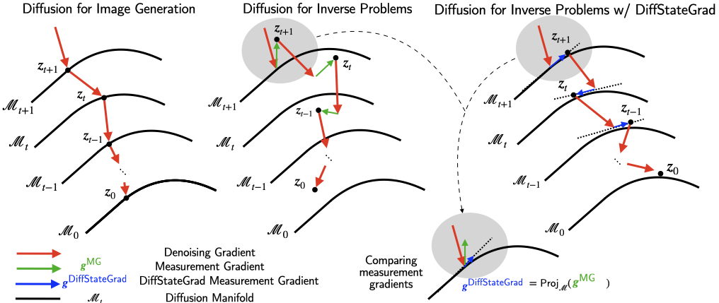
Figure 1: High-level interpretation of Diffusion State-Guided Projected Gradient (DiffStateGrad). DiffStateGrad projects the measurement gradient onto a subspace, defined to capture statistics of the diffusion state at time $t$. This helps the process stay closer to the data manifold during the diffusion process, resulting in better posterior sampling. Without such projection, the measurement gradient pushes the process off the data manifold. The dotted straight line conceptually visualizes the subspace to which the measurement gradient is projected.

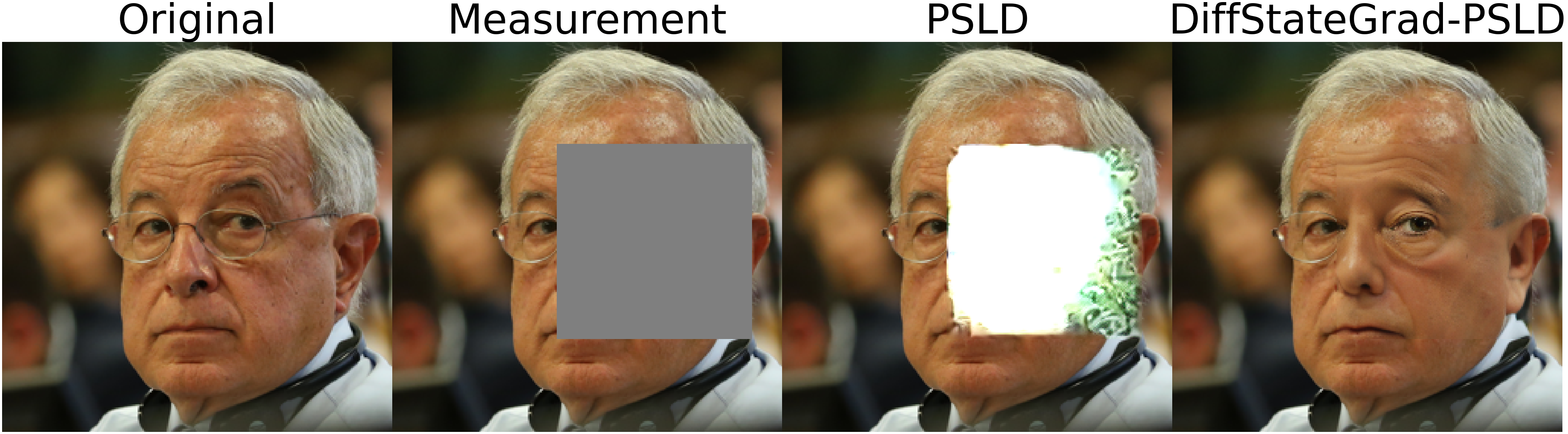
(a) Image visualizations.

(b) PSLD diffusion dynamics.

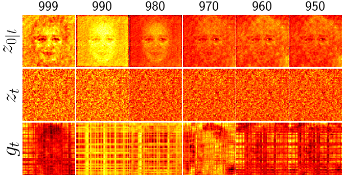
(c) DiffStateGrad-PSLD diffusion dynamics.

Figure 2: Visualization of DiffStateGrad in removing artifacts. The large MG step size pushes the process away from the manifold in PSLD, while DiffStateGrad-PSLD is unaffected. The title refers to the diffusion steps.

Prior works consider sparse priors and provide a theoretical analysis of conditions for the unique recovery of data, a problem known as compressed sensing (Donoho, 2006; Candès et al., 2006). Sparse priors have shown usefulness in medical imaging (Lustig et al., 2007), computational neuroscience (Olshausen & Field, 1997), and engineering applications. This approach is categorized into model-based priors where a structure is assumed on the signal instead of being learned.

Recent literature goes beyond such model-based priors and leverages information from data. The latest works employ generative diffusion models (Song & Ermon, 2019; Kadkhodaie & Simoncelli, 2021), which implicitly learn the data prior $p({\bm{x}})$ by learning a process that transforms noise into samples from a complex data distribution. For inverse problems, this reverse generation process is guided by the likelihood $p({\bm{y}}|{\bm{x}})$, forming a denoiser posterior, to generate data-consistent samples. While diffusion models show state-of-the-art performance, they still face challenges in solving inverse problems.

The main challenge arises since the denoiser posterior, specifically the likelihood component $p({\bm{y}}|{\bm{x}})$, is intractable since the diffusion is trained unconditionally (Song et al., 2021). Prior work addresses this challenge by proposing various approximations or projections to the gradient related to the measurement likelihood $p({\bm{y}}|{\bm{x}})$ to achieve likely solutions (Kawar et al., 2022); when these approximations are not valid, it results in inaccurate posterior sampling and the introduction of “artifacts” in the reconstructed data (Chung et al., 2023). Latent diffusion models (LDMs) (Rombach et al., 2022), due to the nonlinearity of the latent-to-pixel decoder, further exacerbate this challenge. Besides this approximation, the lack of robustness of diffusion models to the measurement gradient step size (Peng et al., 2024) and the measurement noise, and the lack of guarantees for worst-case performance limits their practical applications for inverse problems.

Our contributions: We propose a Diffusion State-Guided Projected Gradient (DiffStateGrad) to address the challenge of staying on the data manifold in solving inverse problems. We focus on gradient-based measurement guidance approaches that use the measurement as guidance to move the intermediate diffusion state ${\bm{x}}_{t}$ toward high-probability regions of the posterior. DiffStateGrad projects the measurement guidance gradient onto a low-rank subspace, capturing the learned prior at time $t$ in the diffusion process (Figure 1). We visualize how the diffusion process is pushed off the manifold when the measurement step size is relatively large in a diffusion model and how the incorporation of DiffStateGrad alleviates this challenge (Figure 2). We perform singular value decomposition (SVD) on the intermediate diffusion state of an image and use the $r$ highest contributing singular vectors as a choice of our projection matrix; by projecting the measurement gradient onto our proposed subspace, we aim to remove the directions orthogonal to the local manifold structure.

• We show that the crucial factor is the choice of the subspace, not the low-rank nature of the subspace projection. We find that our DiffStateGrad projection enhances performance, in contrast to random subspace projections and low-rank approximations of the measurement gradient (Table 1).

• We theoretically prove how DiffStateGrad helps the samples remain on or close to the manifold, hence improving reconstruction quality (Proposition 1).

• We demonstrate that DiffStateGrad increases the robustness of diffusion models to the measurement guidance gradient step size (Figure 6, Table 7) and the measurement noise (Figure 7). For example, for a large step size, DiffStateGrad drastically improves the LPIPS of PSLD (Rout et al., 2023) from $0.463$ to $0.165$ on random inpainting. For large measurement noise, DiffStateGrad improves the SSIM of DAPS (Zhang et al., 2024) from $0.436$ to $0.705$ on box inpainting.

• We empirically show that DiffStateGrad improves the worst-case performance of the diffusion model, e.g., significantly reducing the failure rate (PSNR $<20$) from $26\%$ to $4\%$ on the phase retrieval task, increasing their reliability (Figure 3). DiffStateGrad consistently shows lower standard deviation across the test datasets than state-of-the-art methods.

• We demonstrate that DiffStateGrad significantly improves the performance of state-of-the-art (SOTA) methods, especially in challenging tasks such as phase retrieval and high dynamic range reconstruction. For example, DiffStateGrad improves the PSNR of ReSample (Song et al., 2023a) from $27.61(8.07)$ to $31.19(4.33)$ for phase retrieval, reporting mean (std). Our experiments cover a wide range of linear inverse problems of box inpainting, random inpainting, Gaussian deblur, motion deblur, and super-resolution (Tables 2, 3 and 5) and nonlinear inverse problems of phase retrieval, nonlinear deblur, and high dynamic range (HDR) (Table 4) for image restoration tasks.

Projection Subspace	LPIPS$\downarrow$	SSIM$\uparrow$	PSNR$\uparrow$
No Projection	0.246	0.809	29.05
Random matrix	0.299	0.753	27.30
Measurement gradient	0.242	0.808	29.21
DiffStateGrad (ours)	0.165	0.898	31.68

Table 1: Advantage of diffusion state-guided projection. Results are from random inpainting on FFHQ $256\times 256$.

2 Background & Related Works

Learning-based priors. These methods leverage data structures captured by a pre-trained denoiser (Romano et al., 2017) as plug-and-play priors (Venkatakrishnan et al., 2013), or deep generative models such as variational autoencoders (VAEs)  (Kingma, 2013) and generative adversarial networks (GANs) (Goodfellow et al., 2014) to solve inverse problems (Bora et al., 2017; Ulyanov et al., 2018). The state-of-the-art is based on generative diffusion models, which have shown promising performance in generating high-quality samples in computer vision (Song et al., 2023b), solving PDEs (Shu et al., 2023), and high-energy physics (Shmakov et al., 2024).

Diffusion models. Diffusion models conceptualize the generation of data as the reverse of a noising process, where a data sample ${\bm{x}}_{t}$ at time $t$ within the interval $[0,T]$ follows a specified stochastic differential equation (SDE). This SDE (Song et al., 2021) for the data noising process is described by

$$d{\bm{x}}=-\frac{\beta_{t}}{2}{\bm{x}}\,dt+\sqrt{\beta_{t}}\,d{\bm{w}},$$ (2)

where $\beta_{t}\in(0,1)$ is a positive, monotonically increasing function of time $t$, and ${\bm{w}}$ represents a standard Wiener process. The process begins with an initial data distribution ${\bm{x}}_{0}\sim p_{\text{data}}$ and transitions to an approximately Gaussian distribution ${\bm{x}}_{T}\sim\mathcal{N}(\bm{0},{\bm{I}})$ by time $T$. The objective of regenerating the original data distribution from this Gaussian distribution involves reversing the noising process through a reverse SDE of the form

$$d{\bm{x}}=\left[-\frac{\beta_{t}}{2}{\bm{x}}-\beta_{t}\nabla_{{\bm{x}}_{t}}\log p_{t}({\bm{x}}_{t})\right]dt+\sqrt{\beta_{t}}d\bar{{\bm{w}}},$$ (3)

where $dt$ indicates time moving backward and $\bar{{\bm{w}}}$ is the reversed Wiener process. To approximate $\nabla_{{\bm{x}}_{t}}\log p_{t}({\bm{x}}_{t})$, a neural network $s_{\theta}$ trained via denoising score matching (Vincent, 2011) is used.

Solving inverse problems with diffusion models. Diffusion-based approaches to inverse problems seek to reconstruct the original data ${\bm{x}}_{0}$ from the measurement ${\bm{y}}=\mathcal{A}({\bm{x}}_{0})+{\bm{n}}$. In this case, the reverse SDE implements

$$d{\bm{x}}=\left[-\frac{\beta_{t}}{2}{\bm{x}}-\beta_{t}(\nabla_{{\bm{x}}_{t}}\log{p_{t}({\bm{x}}_{t})}+\nabla_{{\bm{x}}_{t}}\log p_{t}({\bm{y}}|{\bm{x}}_{t}))\right]dt+\sqrt{\beta_{t}}d\bar{{\bm{w}}}.$$ (4)

Conceptually, the learned score function $\nabla_{{\bm{x}}_{t}}\log{p_{t}({\bm{x}}_{t})}$ guides the reverse diffusion process from noise to the data distribution, and the likelihood-related term $\nabla_{{\bm{x}}_{t}}\log p_{t}({\bm{y}}\mid{\bm{x}}_{t})$ ensures measurement consistency. When the model is trained unconditionally, the main challenge is the intractable denoiser posterior due to the lack of an explicit analytical expression for $\nabla_{{\bm{x}}_{t}}\log{p_{t}({\bm{y}}\mid{\bm{x}}_{t})}$; the exact relationship between ${\bm{y}}$ and intermediate states ${\bm{x}}_{t}$ is not well-defined, except at the initial state ${\bm{x}}_{0}$.

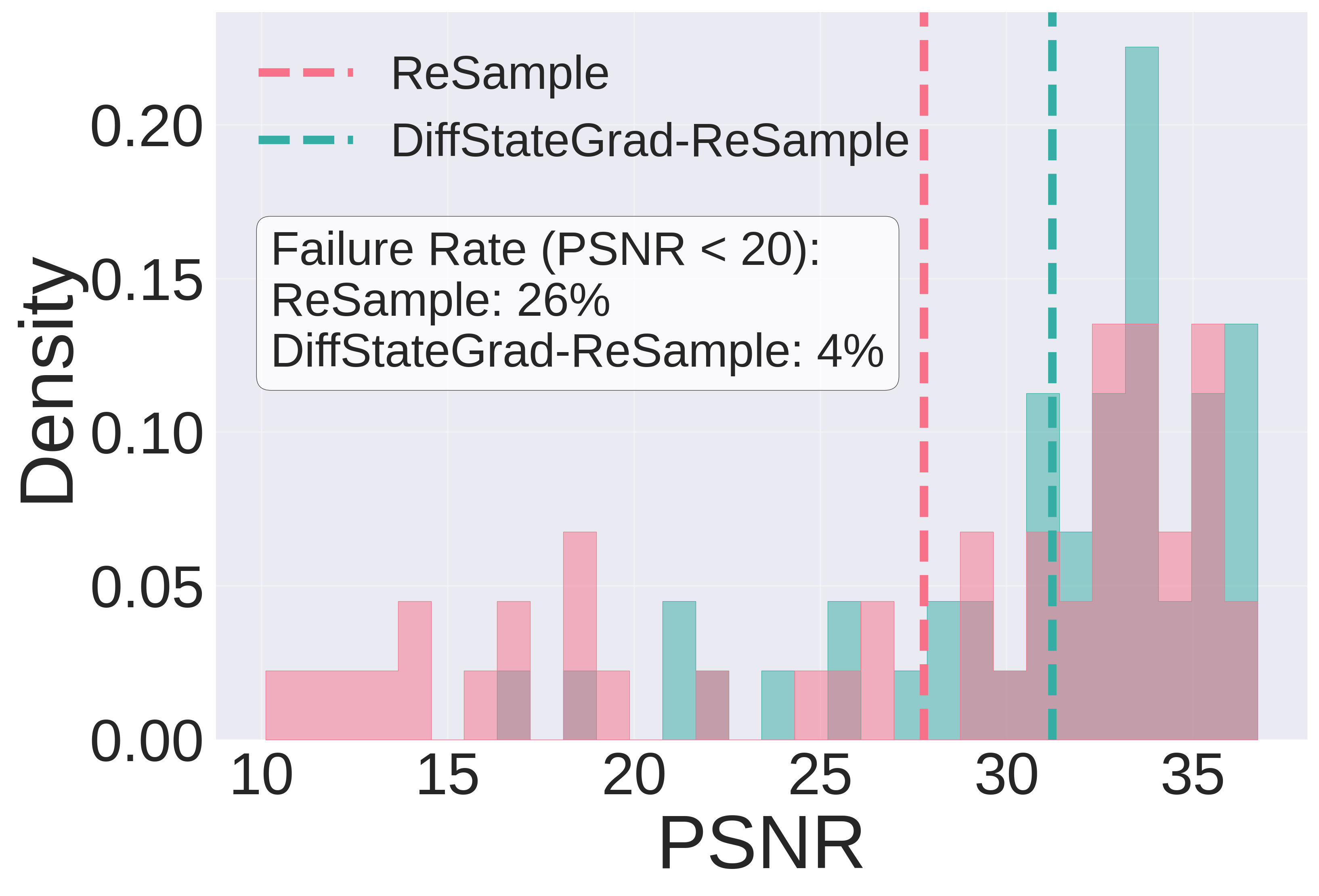
Figure 3: DiffStateGrad improves the worst-case performance. PSNR histogram of ReSample and DiffStateGrad-ReSample for phase retrieval shows that DiffStateGrad-ReSample has a significantly lower failure rate than ReSample.

Solving inverse problems with latent diffusion models. For complex scenarios where direct application of pixel-based models is computationally expensive or ineffective, latent diffusion models (LDMs) offer a promising alternative (Rombach et al., 2022). Given data ${\bm{x}}\in\mathbb{R}^{n}$, the LDM framework utilizes an encoder $\mathcal{E}:\mathbb{R}^{n}\rightarrow\mathbb{R}^{k}$ and a decoder $\mathcal{D}:\mathbb{R}^{k}\rightarrow\mathbb{R}^{n}$, with $k\ll n$, to work in a compressed latent space. ${\bm{x}}_{T}$ is encoded into a latent representation ${\bm{z}}_{T}=\mathcal{E}({\bm{x}}_{T})$ and serves as the starting point for the reverse diffusion process. Then, ${\bm{z}}_{0}$ is decoded to ${\bm{x}}_{0}=\mathcal{D}({\bm{z}}_{0})$, the final reconstruction of the image. Using a latent diffusion model introduces an additional complexity to solving inverse problems. The challenge arises from the nonlinear nature and non-uniqueness mapping of the encoder/decoder, discussed by Rout et al. (2023) in their proposed Posterior Sampling with Latent Diffusion (PSLD); PSLD improves performance by enforcing fixed-point properties on the representations.

Diffusion-based inverse problems addressing challenges of intractable denoiser posterior. To address the intractability of the gradient for the reverse diffusion, Diffusion Posterior Sampling (DPS) (Chung et al., 2023), approximates the probability $p({\bm{y}}\mid{\bm{x}}_{t})\approx p({\bm{y}}|\hat{{\bm{x}}}_{0}\coloneqq\mathbb{E}[{\bm{x}}_{0}\mid{\bm{x}}_{t}])$ using the conditional expectation of the data. Extending to the latent case, Latent-DPS uses $p({\bm{y}}|{\bm{z}}_{t})\approx p({\bm{y}}|\hat{{\bm{x}}}_{0}:=\mathcal{D}(\mathbb{E}[{\bm{z}}_{0}|{\bm{z}}_{t}]))$ (Song et al., 2023a). Two intuitive drawbacks of this approach are that a) the image estimate $\hat{{\bm{x}}}_{0}$ is reconstructed using an expectation, which results in inaccurate estimations for multi-modal complex distributions, and b) the measurement gradient directly updates the noisy state ${\bm{x}}_{t}$, which may push away the state from the desired noise level at $t$.

Prior works aim to address the first challenge by going beyond first-order statistics (Rout et al., 2024) or incorporating posterior covariance into the maximum likelihood estimation step (Peng et al., 2024). Other lines of work address the second issue by decoupling the measurement guidance from the sampling process; they update the data estimate $\hat{{\bm{x}}}_{0}$ at time $t$ using the measurement gradient before resampling it to the noisy manifold (Song et al., 2023a; Zhang et al., 2024). The above-discussed approaches are still highly sensitive to the measurement gradient step size (Peng et al., 2024). Indeed, balancing the measurement gradient with the unconditional score function remains a significant challenge to solving inverse problems using measurement-guided generation. Wu et al. (2024) avoids the discussed approximations and samples from the posterior directly to resolve the need to find a balance between measurement guidance and the prior process.

Projections in diffusion models. Manifold and subspace projections are used in various contexts in diffusion models. He et al. (2024) uses a manifold-preserving approach to improve the efficiency of diffusion generation. Chung et al. (2022) proposes a manifold constraint to project the measurement gradient into the data manifold ${\bm{x}}_{0}$; our proposal is more effective, which projects the measurement gradient on the noisy diffusion state related to ${\bm{x}}_{t}$ or ${\bm{z}}_{t}$ to stay close to $\mathcal{M}_{t}$ rather than $\mathcal{M}_{0}$.

Conditional diffusion models for inverse problems. We focus on unconditional diffusion models as learned priors to solve general inverse problems. This approach leverages already trained diffusion models, which is useful for domains with abundant data. Another approach is to train conditional diffusion models where $\nabla_{{\bm{x}}_{t}}\log p_{t}({\bm{y}}\mid{\bm{x}}_{t})$ is directly captured by the score function, or where the diffusion directly transforms the measurement into the underlying data (e.g., image-to-image diffusion) (Saharia et al., 2022; Liu et al., 2023; Chung et al., 2024). This latter approach is problem-specific; hence, it is not generalizable across inverse tasks.

3 Diffusion State-Guided Projected Gradient (DiffStateGrad)

We propose a Diffusion State-Guided Projected Gradient (DiffStateGrad) to solve general inverse problems. DiffStateGrad can be incorporated into a wide range of diffusion models to improve guidance-based diffusion models. Without loss of generality, we explain DiffStateGrad in the context of Latent-DPS (Chung et al., 2023) and note that DiffStateGrad applies to a wide range of pixel and latent diffusion-based inverse solvers (see Section 4).

Given ${\bm{z}}_{t+1}$, we sample ${\bm{z}}_{t}$ from the unconditional reverse process, and then compute the estimate $\hat{\bm{z}}_{0}({\bm{z}}_{t})\coloneqq\mathcal{D}(\mathbb{E}[{\bm{z}}_{0}\mid{\bm{z}}_{t}])$. Then, the data-consistency guidance term can be incorporated as follows.

$${\bm{z}}_{t}\leftarrow{\bm{z}}_{t}-\eta_{t}\mathcal{P}_{\mathcal{S}_{t}}(\bm{g}_{t}),$$ (5)

where $\bm{g}_{t}=\nabla_{{\bm{z}}_{t+1}}\log p({\bm{y}}\mid\hat{\bm{z}}_{0}({\bm{z}}_{t}))$ is the measurement gradient (MG), $\eta_{t}$ is the step size, and $\mathcal{P}_{\mathcal{S}_{t}}$ is a projection step onto the low-rank subspace $\mathcal{S}_{t}$. The main contribution of this paper is to define this subspace so it results in better posterior sampling; in other words, to define a subspace such that when the measurement gradient is projected onto, the diffusion process is not disturbed and pushed away from the data manifold. We show in Table 1 that indeed the subspace $\mathcal{S}_{t}$, defined by the intermediate diffusion state, results in an improved posterior sampling, unlike a subspace that is constructed based on a random matrix or the low-rank structure of the measurement gradient. Hence, we choose the diffusion state ${\bm{z}}_{t}$ to define $\mathcal{S}_{t}$.

We focus on images as our data modality and implement the projection $\mathcal{P}_{\mathcal{S}_{t}}$ by computing the SVD of ${\bm{z}}_{t}$ in its image matrix form, denoted by $\bm{Z}_{t}$ (i.e., $\bm{U},\bm{S},\bm{V}\leftarrow\text{SVD}(\bm{Z}_{t})$). Then, we compute an adaptive rank $r\leftarrow\underset{k}{\operatorname*{arg\,min}}\{\frac{\sum_{j=1}^{k}s_{j}^{2}}{\sum_{j}s_{j}^{2}}\geq\tau\}$ leveraging a fixed variance retention threshold $\tau$. The gradient $\bm{g}_{t}$, which takes a matrix form for images, is projected onto a subspace defined by the highest $r$ singular values of ${\bm{Z}}_{t}$ as follows:

$$\bm{G}_{t}\leftarrow\bm{U}_{r}\bm{U}_{r}^{\text{T}}\bm{G}_{t}\bm{V}_{r}^{\text{T}}\bm{V}_{r},$$ (6)

where $\bm{G}_{t}$ is the measurement gradient in image matrix form, and $\bm{U}_{r}$ and $\bm{V}_{r}$ contain the first $r$ left and right singular vectors, respectively (Algorithm 1). While we use the full SVD projection (i.e., combining both left and right projection), in practice, one may choose to do either left or right projection. Next, we provide mathematical intuitions (Proposition 1) on the effectiveness of DiffStateGrad in preserving ${\bm{z}}_{t}$, particularly for high-dimensional data with low-rank structure, after the MG update on the manifold $\mathcal{M}_{t}$. Finally, we note that while DiffStateGrad can significantly improve the runtime and computational efficiency of diffusion frameworks that use Adam optimizers for data consistency (Song et al., 2023a; Zhao et al., 2024), the current implementation and this paper does not explore this aspect and, instead, focuses on the property of the proposed subspace.

Algorithm 1 Diffusion State-Guided Projected Gradient (DiffStateGrad) for Latent Diffusion-based Inverse Problems (Image Restoration Tasks)

1:Normal input + variance retention threshold $\tau$

2:Let $T$ = number of total iterations of sampling algorithm and assume we calculate latent image representation ${\bm{Z}}_{t}$ for each iteration. Note that ${\bm{Z}}_{t}$ is a matrix.

3:for $t=T-1$ to $0$ do

4:     Compute measurement gradient $\bm{G}_{t}$ according to sampling algorithm

5:     $\bm{U},\bm{S},\bm{V}\leftarrow\text{SVD}({\bm{Z}}_{t})$ $\triangleright$ Perform SVD on current diffusion state

6:     $\lambda_{j}\leftarrow s_{j}^{2}$ (where $s_{j}$ are the singular values of $\bm{S}$) $\triangleright$ Calculate eigenvalues

7:     $c_{k}\leftarrow\frac{\sum_{j=1}^{k}\lambda_{j}}{\sum_{j}\lambda_{j}}$ $\triangleright$ Cumulative sum of eigenvalues

8:     $r\leftarrow\underset{k}{\operatorname*{arg\,min}}\{c_{k}\geq\tau\}$ $\triangleright$ Determine rank $r$ based on threshold $\tau$

9:     $\bm{A}_{t}\leftarrow\bm{U}_{r}$ $\triangleright$ Get first $r$ left singular vectors

10:     $\bm{B}_{t}\leftarrow\bm{V}_{r}$ $\triangleright$ Get first $r$ right singular vectors

11:     $\bm{R}_{t}\leftarrow\bm{A}_{t}^{T}\bm{G}_{t}\bm{B}_{t}^{T}$ $\triangleright$ Project gradient

12:     $\bm{G}^{\prime}_{t}\leftarrow\bm{A}_{t}\bm{R}_{t}\bm{B}_{t}$ $\triangleright$ Reconstruct approximated gradient

13:     Use updated gradient $\bm{G}^{\prime}_{t}$ in sampling algorithm

14:end for

15:return $\mathcal{D}(\hat{{\bm{z}}}_{0})$

Proposition 1.

Let $\mathcal{M}$ be a smooth $m$-dimensional submanifold of a $d$-dimensional Euclidean space $\mathbb{R}^{d}$, where $m<d$. Assume that for each point ${\bm{z}}_{t}\in\mathcal{M}$, the tangent space $T_{{\bm{z}}_{t}}\mathcal{M}$ is well-defined, and the projection operator $\mathcal{P}_{\mathcal{S}_{{\bm{z}}_{t}}}$ onto an approximate subspace $\mathcal{S}_{{\bm{z}}_{t}}$ closely approximates the projection onto $T_{{\bm{z}}_{t}}\mathcal{M}$. For the state ${\bm{z}}_{t}\in\mathcal{M}$ and the measurement guidance gradient ${\bm{g}}_{t}\in\mathbb{R}^{d}$, consider two update rules:

$${\bm{z}}_{t-1} ={\bm{z}}_{t}-\eta{\bm{g}}_{t}\quad\text{(standard update)},$$ (7)

$${\bm{z}}_{t-1}^{\prime} ={\bm{z}}_{t}-\eta\mathcal{P}_{\mathcal{S}_{{\bm{z}}_{t}}}({\bm{g}}_{t})\quad\text{(projected update)},$$

where $\eta>0$ is a small step size.

Then, for sufficiently small $\eta$, the projected update ${\bm{z}}_{t-1}^{\prime}$ stays closer to the manifold $\mathcal{M}$ than the standard update ${\bm{z}}_{t-1}$. That is,

$$\text{dist}({\bm{z}}_{t-1}^{\prime},\mathcal{M})<\text{dist}({\bm{z}}_{t-1},\mathcal{M}).$$ (8)

The remainder of this section provides intuitions on how DiffStateGrad improves solving inverse problems in the presence of a suitable learned prior. Let the initial latent state ${\bm{z}}_{t}$ be on the manifold $\mathcal{M}_{t}$ (e.g., being artifact-free, as the diffusion model is trained on clean data samples). We observe that pushing away from the manifold process (e.g., introducing artifacts) can only be introduced via the guidance by the data-consistency gradient step, as this is the sole mechanism by which information from the measurement process enters the latent space. Consider the manifold $\mathcal{M}$ of artifact-free latent representations. Each ${\bm{z}}_{t}$ lies on this manifold, and the tangent space $T_{{\bm{z}}_{t}}\mathcal{M}$ represents the directions of “allowable” updates that maintain the artifact-free property staying on the current manifold.

Our DiffStateGrad method, through the projection operator $\mathcal{P}_{\mathcal{S}_{t}}$, approximates this tangent space. The effectiveness of DiffStateGrad depends on how well $\mathcal{P}_{\mathcal{S}_{t}}$ approximates the projection onto $T_{{\bm{z}}_{t}}\mathcal{M}$. Hence, we discuss a rationale on how the approximated projection is sufficient for performance; we, accordingly, support this by experimental results in Section 4. First, the SVD captures the principal directions of variation in ${\bm{z}}_{t}$, which are likely to align with the local structure of the manifold when the data is high-dimensional. Second, by adaptively choosing the rank based on a variance retention threshold, we ensure that the projection preserves the most significant state-related structural information while filtering out potential noise or artifact-inducing components from the measurement gradient. Finally, the low-rank nature of our approximation aligns with the assumption that the manifold of representations has a lower intrinsic dimensionality than the ambient space.

Hence, by projecting the measurement gradient onto this subspace defined by the current latent state ${\bm{z}}_{t}$, we effectively filter the directions orthogonal to the local manifold structure, and hence, remove artifacts-inducing components. This projection ensures that updates to ${\bm{z}}_{t}$ remain closer to the manifold $\mathcal{M}$ than unprojected updates would, as stated in Proposition 1. Consequently, DiffStateGrad relies on the reliability of the learned prior and helps to provide high-probability posterior samples. This creates an inductive process: if ${\bm{z}}_{t}$ is artifact-free, and we only allow updates that align with its structure (i.e., updates that stay close to the manifold $\mathcal{M}$), subsequent latent representation ${\bm{z}}_{t}$ will likely be samples from the high-probability regions of the posterior.

Figure 2 demonstrates the effectiveness of DiffStateGrad in removing artifacts when the MG step size is large; artifacts are introduced onto the measurement gradient and stay within the latent representation in PSLD (Rout et al., 2023). On the other hand, the reverse process via DiffStateGrad-PSLD (our method applied to PSLD) stays artifact-free, consistent with the mathematical analysis in Proposition 1 and the practical efficacy of the proposed SVD-based subspace projection. Finally, we note that the most significant improvements appear in challenging tasks such as phase retrieval, HDR, and inpainting. We attribute the effectiveness of DiffStateGrad, particularly in challenging tasks, to a reduced rate of failure cases (Figure 3). By constraining solutions closer to the data manifold, DiffStateGrad minimizes extreme failures, enhances consistency in reconstruction quality, and improves overall performance metrics.

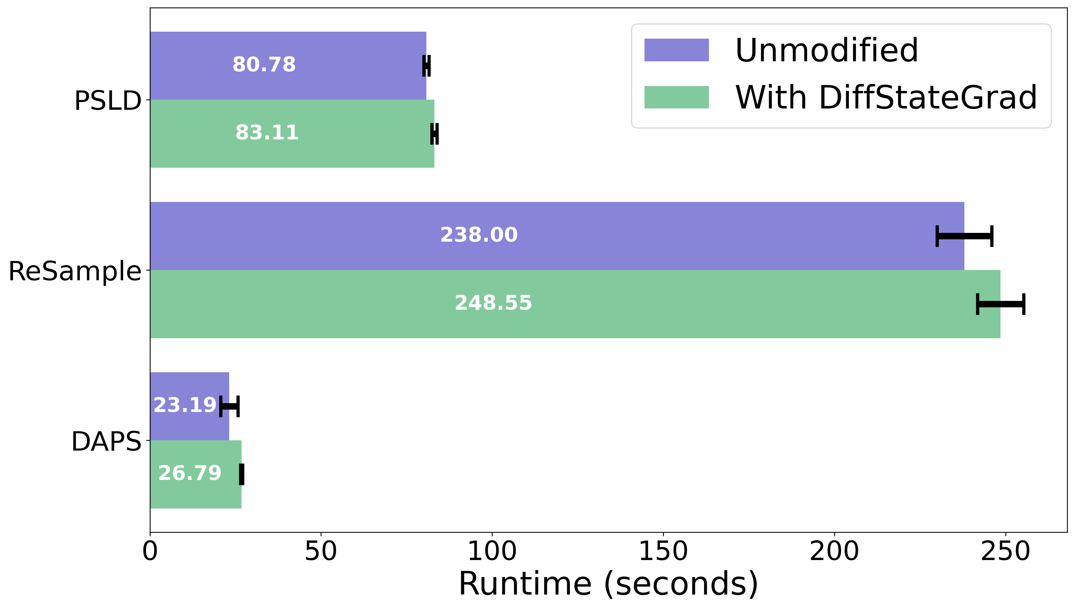
Figure 4: Runtime complexity of DiffStateGrad. The increase of runtime with DiffStateGrad is minimal.

3.1 Efficiency

DiffStateGrad introduces minimal computational overhead. We perform SVD at most once per iteration, and for latent diffusion solvers, this occurs in the latent space on $64\times 64$ matrices. By selecting a low rank based on a variance threshold, subsequent projection and reconstruction operations are performed on reduced matrices, further decreasing computational complexity. Figure 4 illustrates the runtime for the three diffusion-based methods of PSLD (Rout et al., 2023), ReSample (Song et al., 2023a), and DAPS (Zhang et al., 2024) with and without DiffStateGrad. The figure shows that the additional computational cost of incorporating DiffStateGrad is marginal, typically adding only a few seconds to the total runtime (see Section C.2 for further details). We note that our method is not intended to improve efficiency, but rather to enhance performance and robustness.

4 Results

This section provides extensive experimental results on the effectiveness of DiffStateGrad employed in several methods for image-based inverse problems. We show that DiffStateGrad significantly improves (1) the robustness of diffusion-based methods to the choice of measurement gradient step size and measurement noise, and (2) the overall posterior sampling performance of diffusion.

4.1 Experimental Setup

We evaluate the performance of DiffStateGrad applied to three SOTA diffusion methods of PSLD (Rout et al., 2023), ReSample (Song et al., 2023a), and DAPS (Zhang et al., 2024). These methods span both latent solvers (PSLD and ReSample) and pixel-based solvers (DAPS). We evaluate their performance based on key quantitative metrics, including LPIPS (Learned Perceptual Image Patch Similarity), PSNR (Peak Signal-to-Noise Ratio), and SSIM (Structural Similarity Index) (Wang et al., 2004). We demonstrate the effectiveness of DiffStateGrad on two datasets: a) the FFHQ $256\times 256$ validation dataset (Karras et al., 2021), and b) the ImageNet $256\times 256$ validation dataset (Deng et al., 2009). For pixel-based experiments, we use (i) the pre-trained diffusion model from (Chung et al., 2023) for the FFHQ dataset, and (ii) the pre-trained model from (Dhariwal & Nichol, 2021) for the ImageNet dataset. For latent diffusion experiments, we use (i) the unconditional LDM-VQ-4 model trained on FFHQ (Rombach et al., 2022) for the FFHQ dataset, and (ii) the Stable Diffusion v1.5 (Rombach et al., 2022) model for the ImageNet dataset.

We consider both linear and nonlinear inverse problems for natural images. For evaluation, we sample a fixed set of $100$ images from the FFHQ and ImageNet validation sets. Images are normalized to the range $[0,1]$. We use the default settings for PSLD, ReSample, and DAPS for all experiments (see Appendix C for more details).

For linear inverse problems, we consider (1) box inpainting, (2) random inpainting, (3) Gaussian deblur, (4) motion deblur, and (5) super-resolution. In the box inpainting task, a random $128\times 128$ box is used, while the random inpainting task employs a $70\%$ random mask. Gaussian and motion deblurring tasks utilize kernels of size $61\times 61$, with standard deviations of $3.0$ and $0.5$, respectively. For super-resolution, images are downscaled by a factor of $4$ using a bicubic resizer. For nonlinear inverse problems, we consider (1) phase retrieval, (2) nonlinear deblur, and (3) high dynamic range (HDR). For phase retrieval, we use an oversampling rate of 2.0, and due to the instability and non-uniqueness of reconstruction, we adopt the strategy from DPS (Chung et al., 2023) and DAPS (Zhang et al., 2024), generating four separate reconstructions and reporting the best result. Like DAPS (Zhang et al., 2024), we normalize the data to lie in the range [0, 1] before applying the discrete Fourier transform. For nonlinear deblur, we use the default setting from (Tran et al., 2021). For HDR, we use a scale factor of 2. We note that PSLD is not designed to handle nonlinear inverse problems.

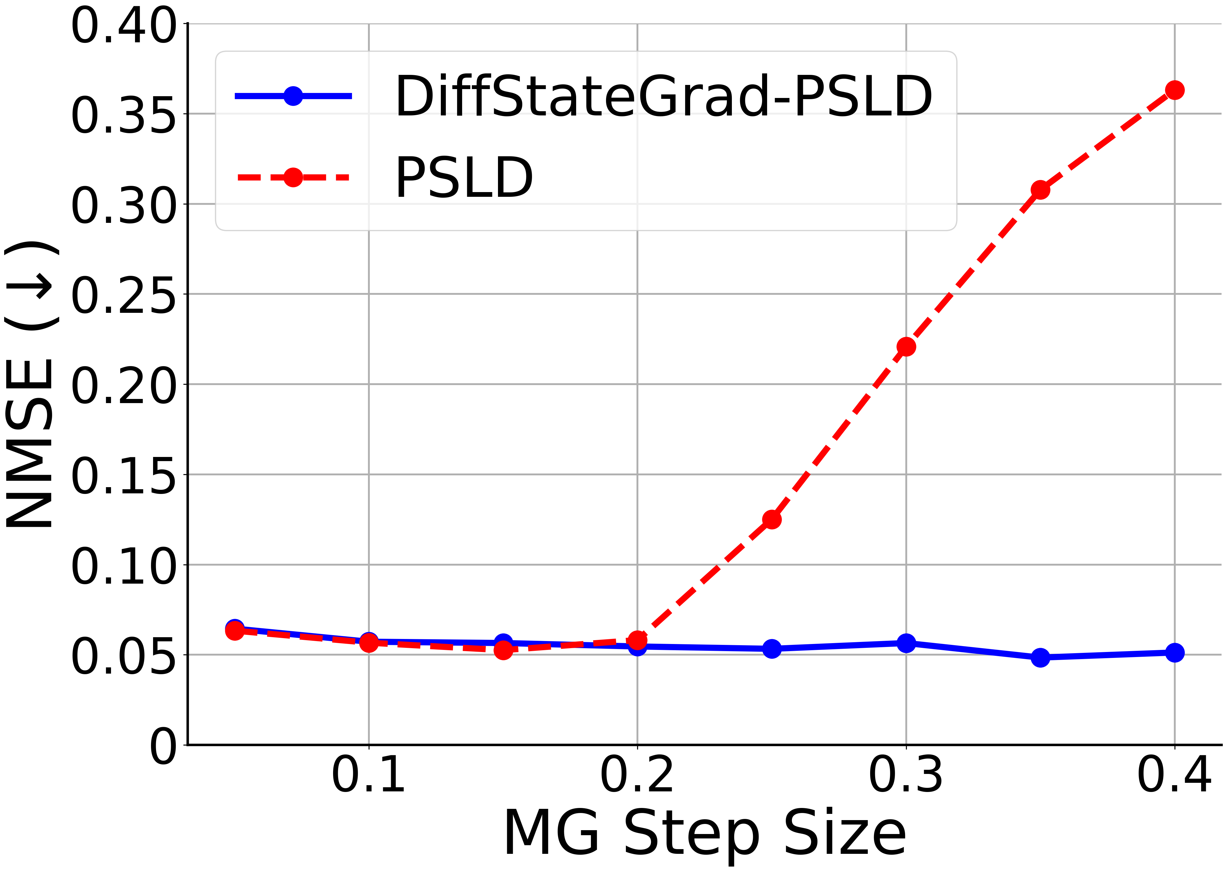
(a) Box Inpainting (NMSE).

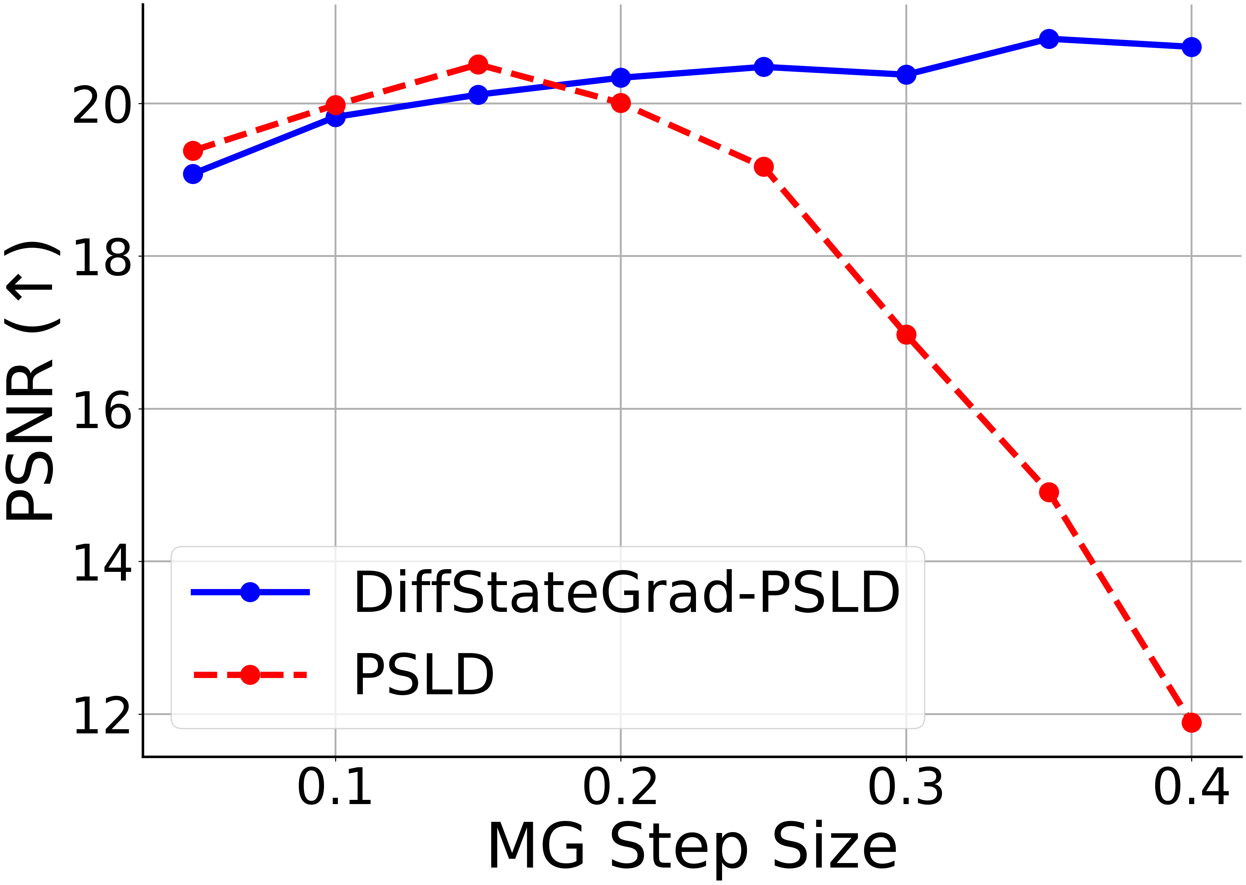
(b) Box Inpainting (PSNR).

(c) Random Inpainting (LPIPS).

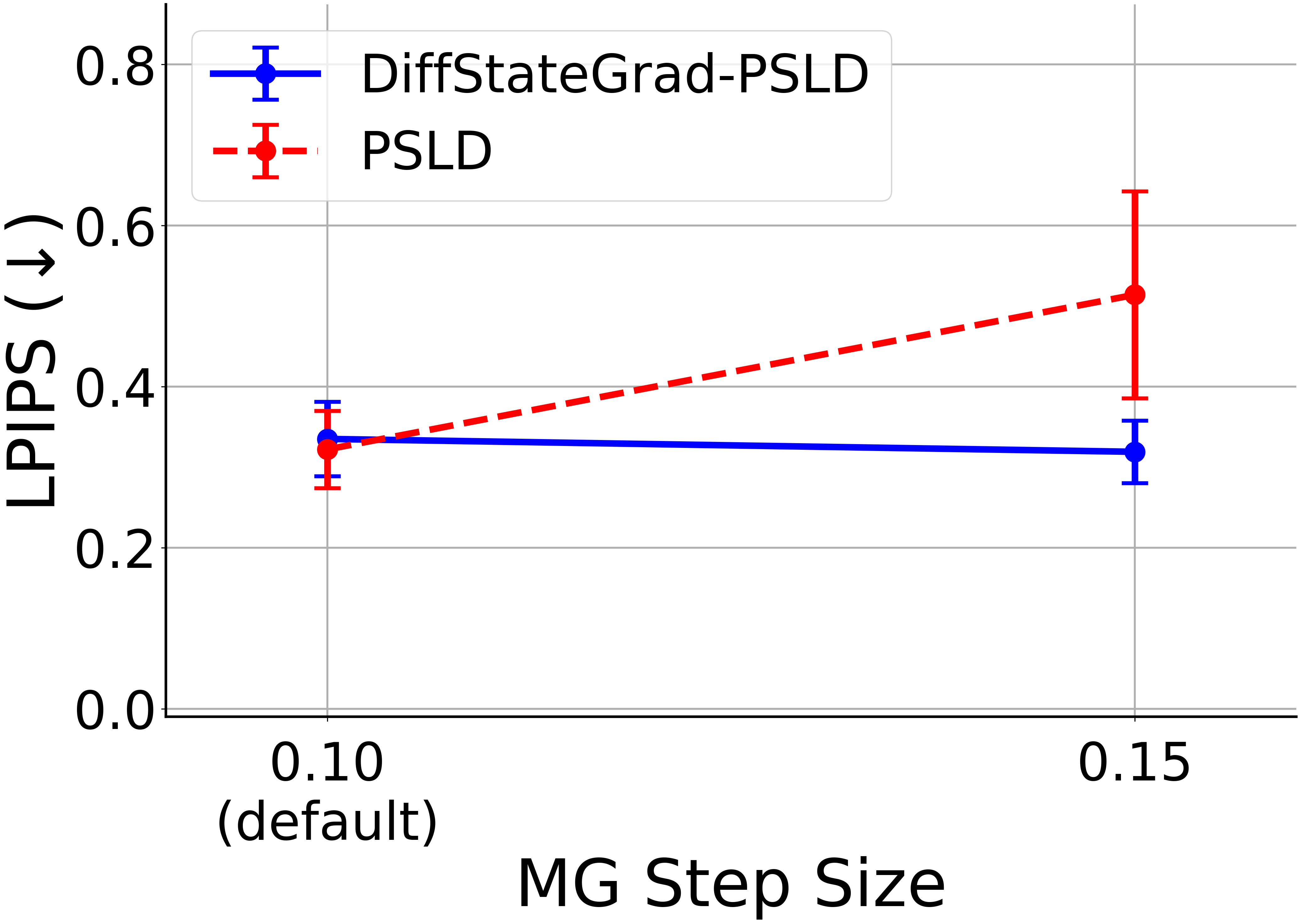
(d) Motion Deblur (LPIPS).

(e) Super-Resolution (LPIPS).

Figure 6: Robustness of DiffStateGrad to MG step size. (a-b) Performance on box inpainting across various MG step sizes. (c-e) Performance on different tasks with default and large step sizes. We evaluate the performance of PSLD and DiffStateGrad-PSLD using FFHQ $256\times 256$.

(a) Inpainting (Box).

(b) Gaussian Deblur.

Figure 7: Robustness of DiffStateGrad to measurement noise. We evaluate the performance of DiffStateGrad-PSLD and PSLD-DAPS with their respective counterparts on different tasks across a range of measurement noise levels using FFHQ $256\times 256$.

4.2 Robustness

Figure 6 exhibits the sensitivity of PSLD to the choice of MG step size; the performance of PSLD significantly deteriorates when a relatively large MG step size is used, leading to poor results across all tasks. In contrast, DiffStateGrad-PSLD shows superior robustness, maintaining high performance over a wide range of MG step sizes. Figure 7 demonstrates the robustness of DiffStateGrad methods compared to their non-DiffStateGrad counterparts when faced with increasing measurement noise. For both inpainting and Gaussian deblur tasks, the performance of DAPS and PSLD deteriorates significantly as noise levels rise. In contrast, DiffStateGrad-DAPS and DiffStateGrad-PSLD exhibit superior resilience across the range of noise levels tested.

Table 2: Performance comparison for inpainting tasks on FFHQ 256 $\times$ 256.

Method	Inpaint (Box)			Inpaint (Random)
	LPIPS$\downarrow$	SSIM$\uparrow$	PSNR$\uparrow$	LPIPS$\downarrow$	SSIM$\uparrow$	PSNR$\uparrow$
Pixel-based
DAPS	0.136 (0.027)	0.806 (0.028)	24.57 (2.61)	0.130 (0.022)	0.829 (0.022)	30.79 (1.60)
DiffStateGrad-DAPS (ours)	0.113 (0.020)	0.849 (0.029)	24.78 (2.62)	0.099 (0.020)	0.887 (0.023)	32.04 (1.79)
Latent
PSLD	0.158 (0.023)	0.819 (0.031)	24.22 (2.80)	0.246 (0.053)	0.809 (0.049)	29.05 (1.98)
DiffStateGrad-PSLD (ours)	0.092 (0.019)	0.880 (0.028)	24.32 (2.78)	0.165 (0.035)	0.898 (0.024)	31.68 (1.74)
ReSample	0.198 (0.032)	0.807 (0.036)	19.91 (1.78)	0.115 (0.028)	0.892 (0.030)	31.27 (2.35)
DiffStateGrad-ReSample (ours)	0.156 (0.027)	0.841 (0.032)	23.59 (2.38)	0.106 (0.023)	0.913 (0.023)	31.91 (1.84)

Table 3: Performance comparison for deblurring and super-resolution tasks on FFHQ 256 $\times$ 256.

Method	Gaussian deblur		Motion deblur		SR (x4)
	LPIPS$\downarrow$	PSNR$\uparrow$	LPIPS$\downarrow$	PSNR$\uparrow$	LPIPS$\downarrow$	PSNR$\uparrow$
Pixel-based
DAPS	0.216 (0.045)	27.92 (1.90)	0.154 (0.030)	30.13 (1.70)	0.197 (0.032)	28.64 (1.69)
DiffStateGrad-DAPS (ours)	0.180 (0.031)	29.02 (1.86)	0.119 (0.023)	31.74 (1.57)	0.181 (0.028)	29.35 (1.70)
Latent
PSLD	0.357 (0.060)	22.87 (1.67)	0.322 (0.048)	24.25 (1.47)	0.313 (0.098)	24.51 (2.98)
DiffStateGrad-PSLD (ours)	0.355 (0.043)	22.95 (1.32)	0.319 (0.039)	24.31 (1.18)	0.320 (0.079)	24.56 (2.46)
ReSample	0.253 (0.039)	27.78 (1.79)	0.160 (0.028)	30.55 (1.75)	0.204 (0.038)	28.02 (2.05)
DiffStateGrad-ReSample (ours)	0.245 (0.030)	28.04 (1.66)	0.153 (0.024)	30.82 (1.71)	0.200 (0.031)	28.27 (1.84)

4.3 Performance

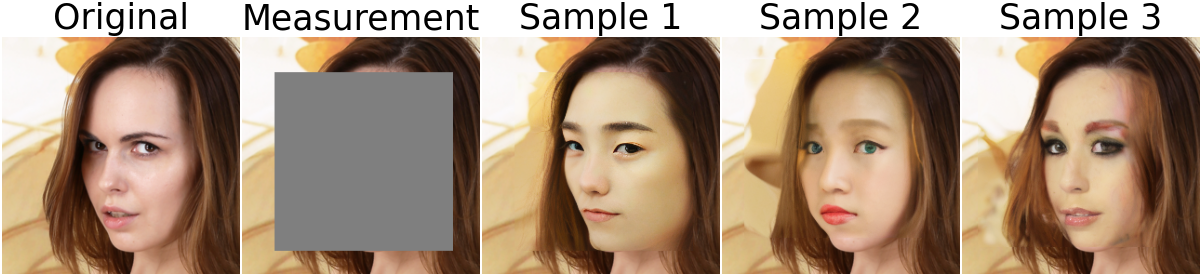
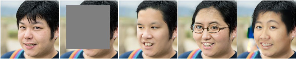
(a) Box inpainting ($192\times 192$ box).

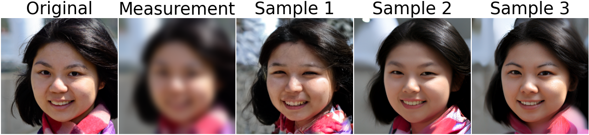
(b) Gaussian deblur ($81\times 81$ kernel, SD of 7).

Figure 15: Reconstruction diversity of DiffStateGrad. DiffStateGrad-PSLD with a large MG step size can produce a diverse range of images from multimodal posteriors. Generated images have distinctive facial features.

We provide quantitative results in Tables 2, 3, 4 and 5, and qualitative results in Figure 9. These results demonstrate the substantial improvement in the performance of DiffStateGrad-PSLD, DiffStateGrad-ReSample, and DiffStateGrad-DAPS against their respective SOTA counterparts across a wide variety of linear and nonlinear tasks on both FFHQ and ImageNet. For example, DiffStateGrad significantly improves performance and increases reconstruction consistency in both pixel-based and latent solvers for phase retrieval (Table 4). We additionally show that DiffStateGrad does not impact the diversity of the posterior sampling (see Figure 15). Finally, we note that DiffStateGrad is robust to the choice of subspace rank (Figures 10 and 8). We refer the reader to Appendix B for the extensive qualitative performance of DiffStateGrad.

Table 4: Performance comparison for nonlinear tasks on FFHQ 256 $\times$ 256.

Method	Phase retrieval		Nonlinear deblur		High dynamic range
	LPIPS$\downarrow$	PSNR$\uparrow$	LPIPS$\downarrow$	PSNR$\uparrow$	LPIPS$\downarrow$	PSNR$\uparrow$
Pixel-based
DAPS	0.139 (0.026)	30.52 (2.61)	0.184 (0.032)	27.80 (1.97)	0.170 (0.075)	26.91 (3.94)
DiffStateGrad-DAPS (ours)	0.105 (0.023)	32.25 (1.34)	0.145 (0.027)	29.51 (2.16)	0.143 (0.070)	27.76 (3.18)
Latent
ReSample	0.237 (0.189)	27.61 (8.07)	0.188 (0.037)	29.54 (1.89)	0.190 (0.067)	24.88 (3.46)
DiffStateGrad-ReSample (ours)	0.154 (0.104)	31.19 (4.33)	0.185 (0.035)	29.91 (1.60)	0.164 (0.041)	25.50 (3.07)

Table 5: Performance comparison for linear tasks on ImageNet 256 $\times$ 256.

Method	Gaussian deblur		Motion deblur		SR (x4)
	LPIPS$\downarrow$	PSNR$\uparrow$	LPIPS$\downarrow$	PSNR$\uparrow$	LPIPS$\downarrow$	PSNR$\uparrow$
PSLD	0.466 (0.085)	20.70 (3.01)	0.435 (0.102)	21.26 (3.44)	0.416 (0.063)	22.29 (3.08)
DiffStateGrad-PSLD (ours)	0.446 (0.076)	22.34 (3.19)	0.399 (0.060)	23.80 (3.27)	0.370 (0.081)	23.53 (3.52)

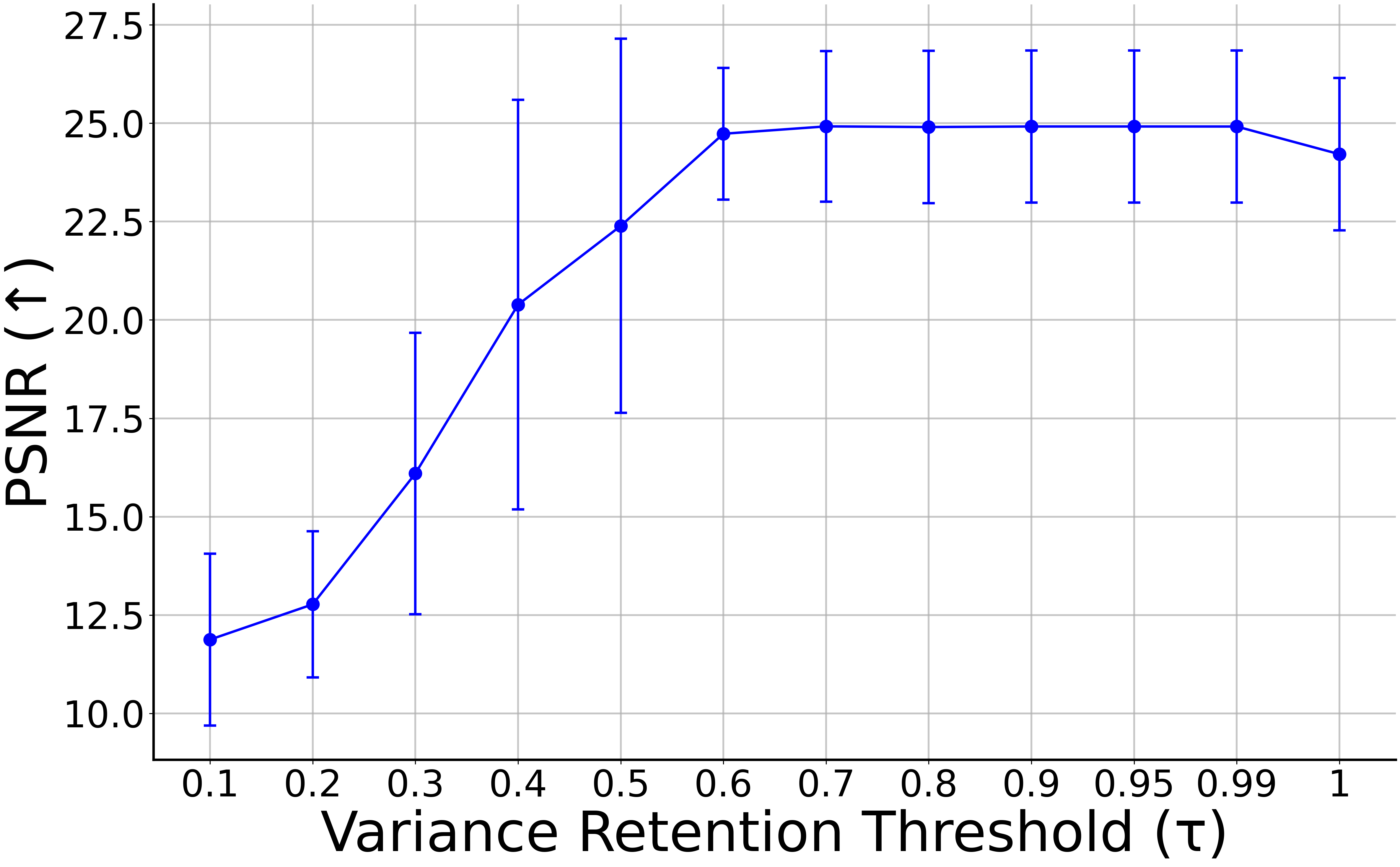
(a) PSNR

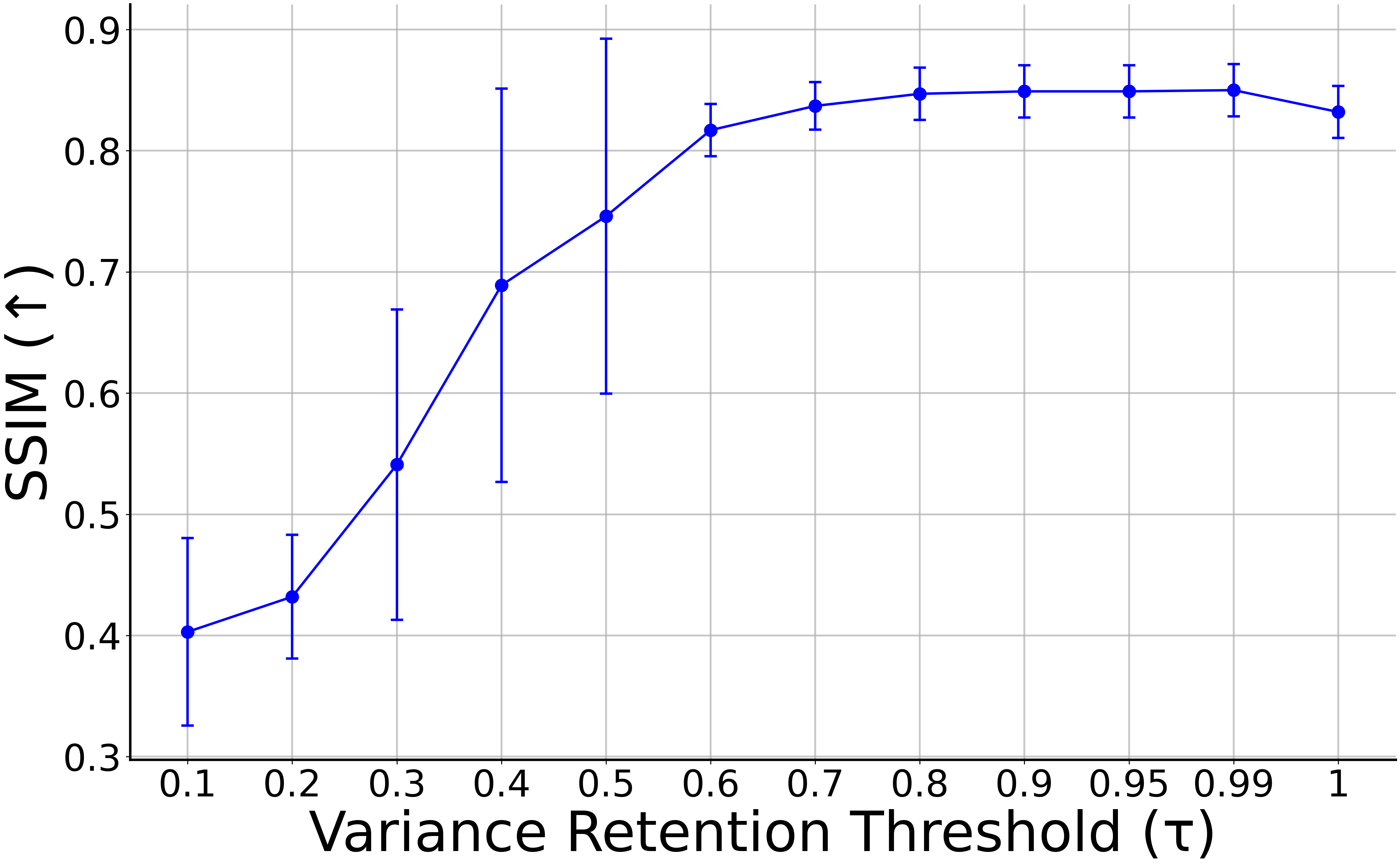
(b) SSIM

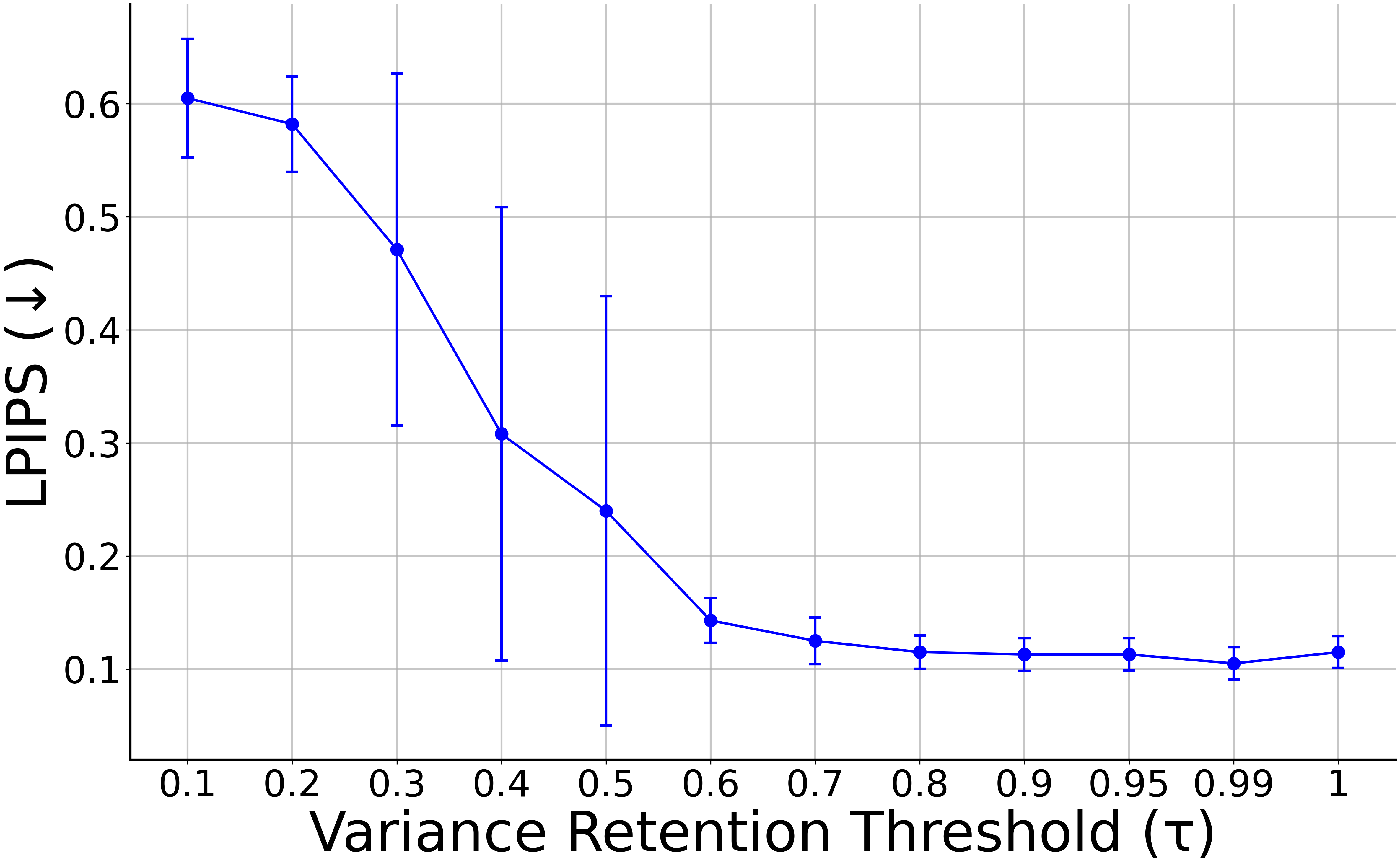
(c) LPIPS

Figure 8: Performance of DiffStateGrad-DAPS for different variance retention thresholds $\tau$. DiffStateGrad is robust to the choice of $\tau$, as values $\geq 0.6$ show similar performance in this figure. In our main experiments, we use $\tau=0.99$ (see Section C.1 for further details). We evaluate images from FFHQ $256\times 256$ on box inpainting.

5 Conclusion

We introduce a Diffusion State-Guided Projected Gradient (DiffStateGrad) to enhance the performance and robustness of diffusion models in solving inverse problems. DiffStateGrad addresses the introduction of artifacts and deviations from the data manifold by constraining gradient updates to a subspace approximating the manifold. DiffStateGrad is versatile, applicable across various diffusion models and sampling algorithms, and includes an adaptive rank that dynamically adjusts to the gradient’s complexity. Overall, DiffStateGrad reduces the need for excessive tuning of hyperparameters and significantly boosts performance for more challenging inverse problems.

We note that DiffStateGrad assumes that the learned prior is a relatively good prior for the task at hand. Since DiffStateGrad encourages the process to stay close to the manifold structure captured by the generative prior, it may introduce the prior’s biases into image restoration tasks. Hence, DiffStateGrad may not be recommended for certain inverse problems such as black hole imaging (Feng et al., 2024).

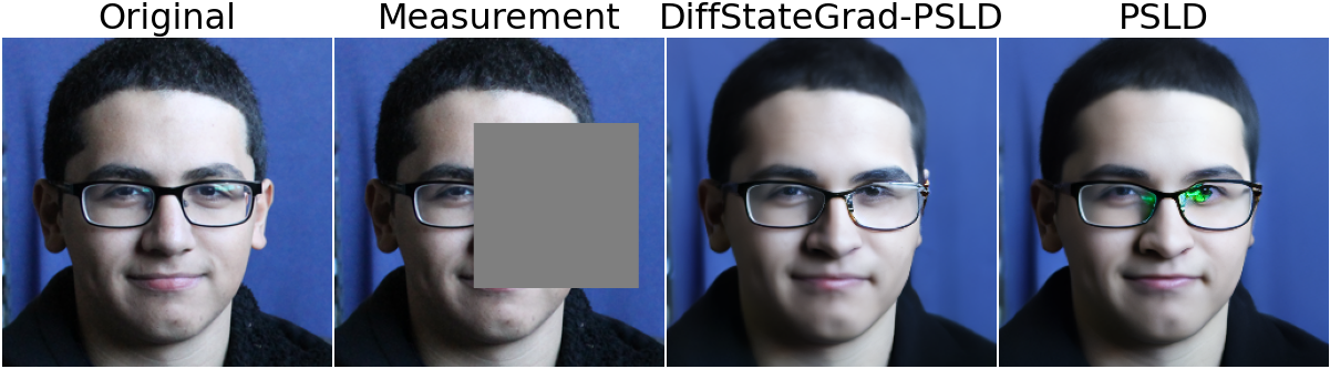
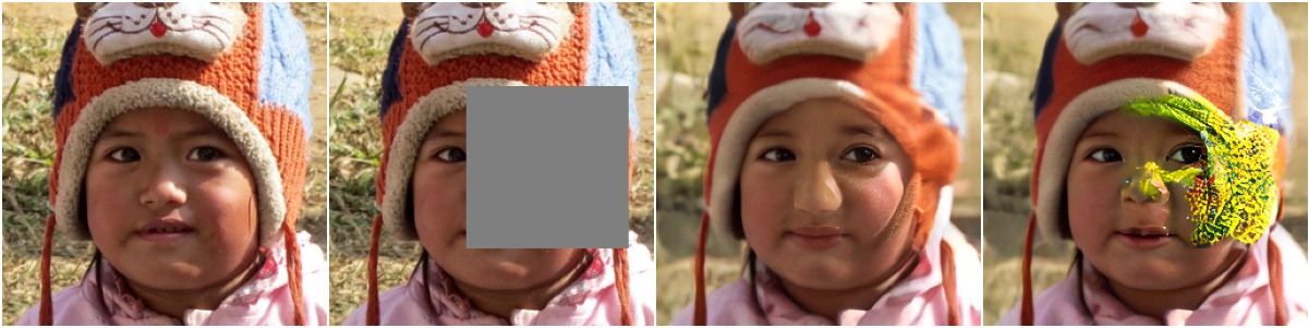
(a) Box inpainting.

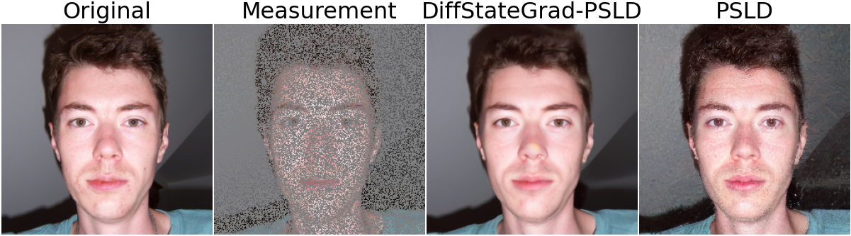
(b) Random inpainting.

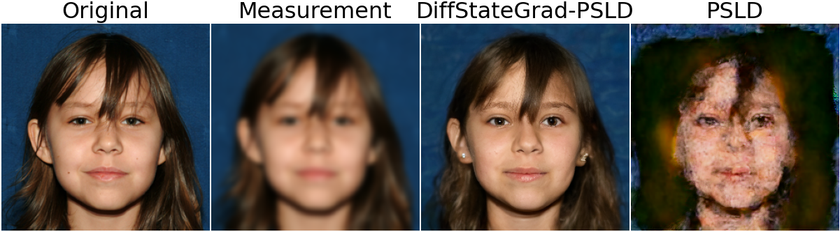
(c) Gaussian deblur.

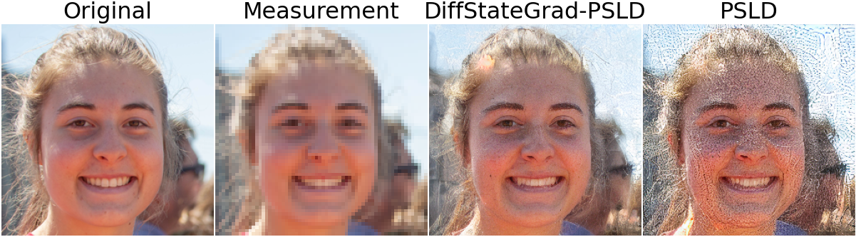
(d) Super-resolution ($\times 4$).

Figure 9: Qualitative comparison of DiffStateGrad-PSLD and PSLD for their best-performing MG step size. DiffStateGrad-PSLD can remove artifacts and reduce failure cases, producing more reliable reconstructions. Images are chosen at random for visualization.

6 Reproducibility Statement

To ensure the reproducibility of our results, we thoroughly detail the hyperparameters used in our experiments in Section C.1. We also provide specific implementation and configuration details of all the baselines used in Sections C.3, C.4 and C.5. Moreover, we use easily accessible pre-trained diffusion models throughout our experiments. PSLD (https://github.com/LituRout/PSLD), ReSample (https://github.com/soominkwon/resample), and DAPS (https://github.com/zhangbingliang2019/DAPS) all have publicly available code. We will make the anonymous GitHub repository with our code available to the reviewers after the discussion forum opens.

Appendix A Additional Results

This section provides additional results.

Table 6: Performance comparison for inpainting tasks on ImageNet 256 $\times$ 256.

Method	Inpaint (Box)			Inpaint (Random)
	LPIPS$\downarrow$	SSIM$\uparrow$	PSNR$\uparrow$	LPIPS$\downarrow$	SSIM$\uparrow$	PSNR$\uparrow$
PSLD	0.182 (0.033)	0.780 (0.044)	16.28 (3.49)	0.217 (0.073)	0.846 (0.070)	26.56 (2.98)
DiffStateGrad-PSLD (ours)	0.176 (0.030)	0.803 (0.045)	18.90 (3.82)	0.169 (0.050)	0.878 (0.051)	28.48 (4.04)

Table 7: Robustness comparison of PSLD and DiffStateGrad-PSLD on linear tasks under different MG step sizes on FFHQ 256 $\times$ 256.

Method	Inpaint (Box)		Inpaint (Random)		Gaussian deblur		Motion deblur		SR (×4)
	LPIPS$\downarrow$	PSNR$\uparrow$	LPIPS$\downarrow$	PSNR$\uparrow$	LPIPS$\downarrow$	PSNR$\uparrow$	LPIPS$\downarrow$	PSNR$\uparrow$	LPIPS$\downarrow$	PSNR$\uparrow$
Default MG step size
PSLD	0.158	24.22	0.246	29.05	0.357	22.87	0.322	24.25	0.313	24.51
DiffStateGrad-PSLD (ours)	0.095	23.76	0.265	28.14	0.366	22.24	0.335	23.34	0.392	22.12
Large MG step size
PSLD	0.252	11.99	0.463	20.62	0.549	17.47	0.514	18.81	0.697	7.700
DiffStateGrad-PSLD (ours)	0.092	24.32	0.165	31.68	0.355	22.95	0.319	24.31	0.320	24.56

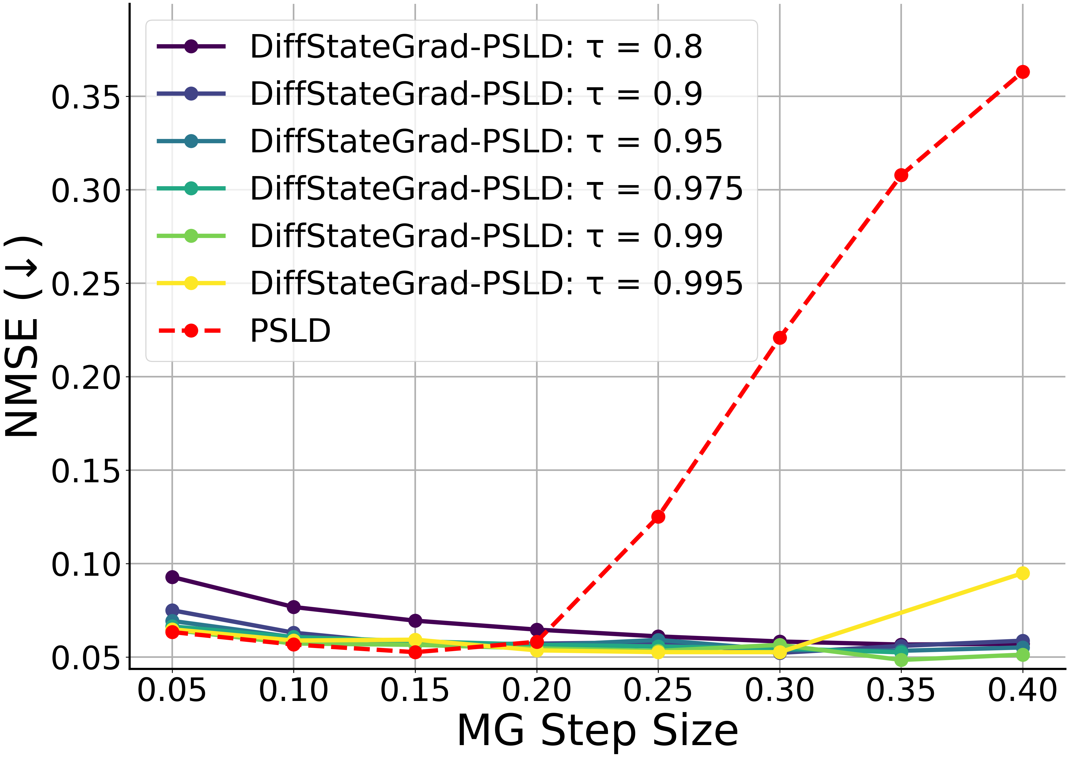
(a) NMSE

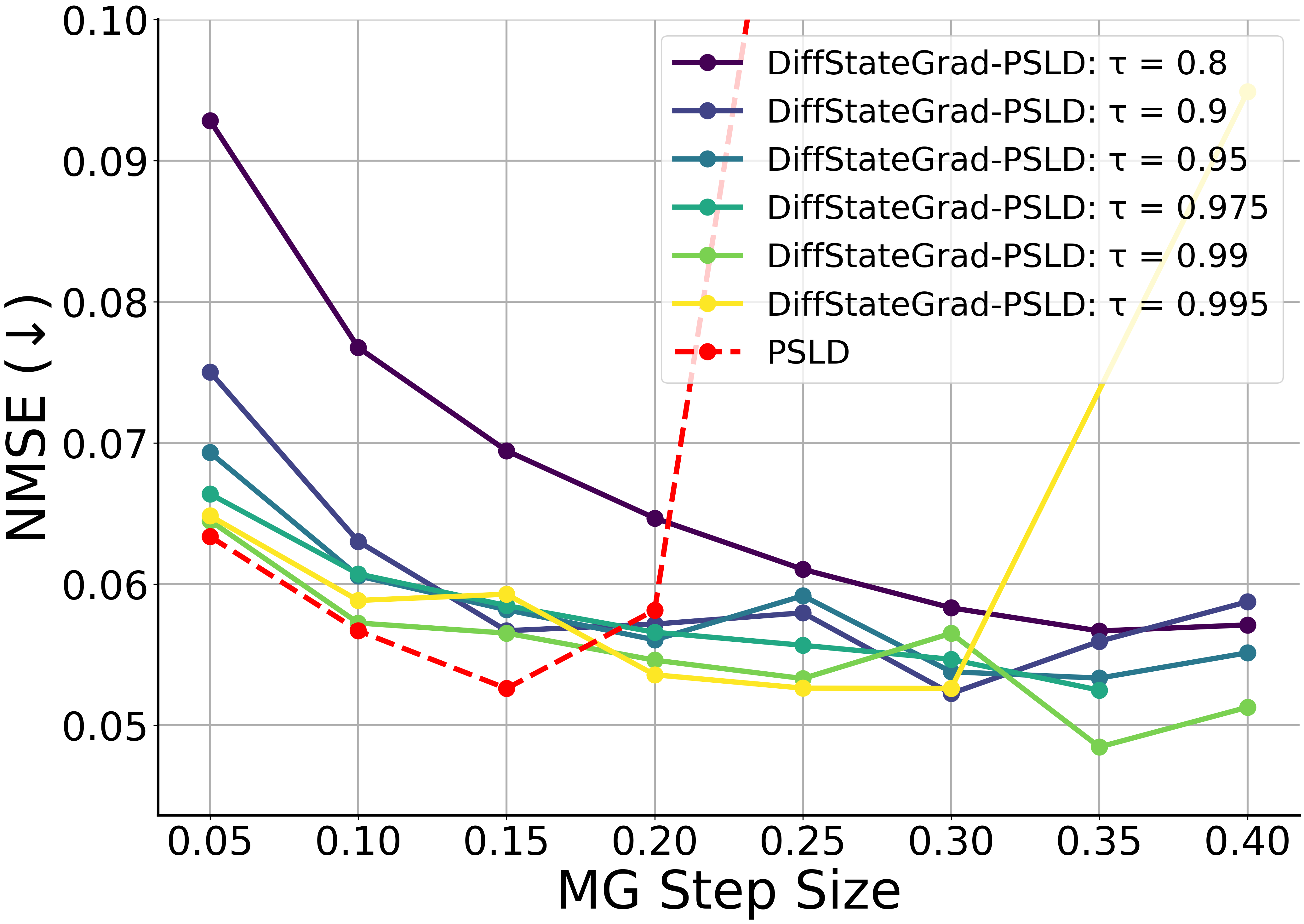
(b) NMSE (zoomed)

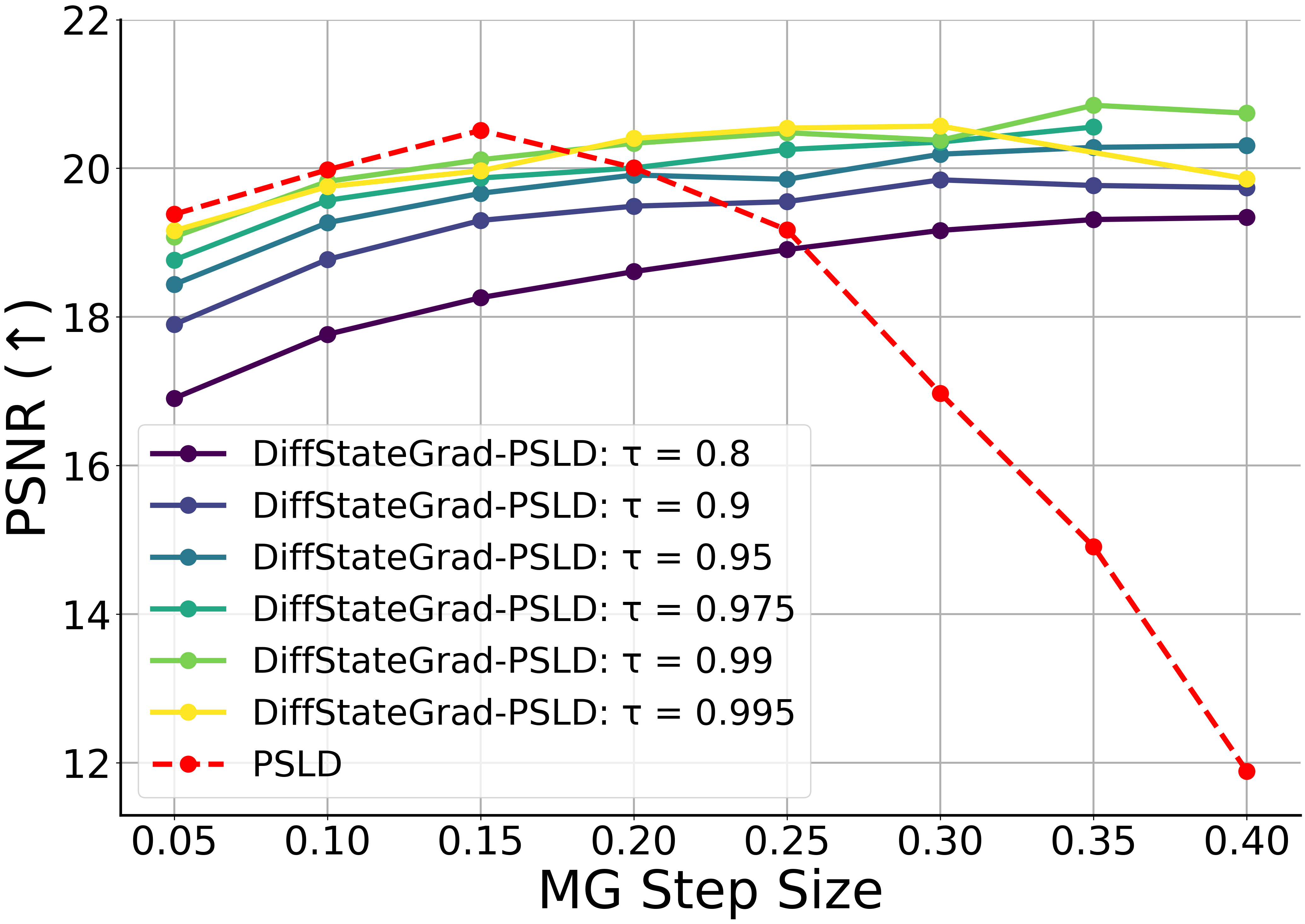
(c) PSNR

Figure 10: Robustness comparison of PSLD and DiffStateGrad-PSLD for different variance retention thresholds $\tau$. We evaluate images from FFHQ $256\times 256$ on box inpainting.

Table 8: SSIM comparison for deblurring and super-resolution tasks on FFHQ 256 $\times$ 256.

Method	Gaussian deblur	Motion deblur	SR (x4)
	SSIM$\uparrow$	SSIM$\uparrow$	SSIM$\uparrow$
Pixel-based
DAPS	0.786 (0.051)	0.837 (0.040)	0.797 (0.044)
DiffStateGrad-DAPS (ours)	0.803 (0.044)	0.853 (0.028)	0.801 (0.039)
Latent
PSLD	0.537 (0.094)	0.615 (0.075)	0.650 (0.140)
DiffStateGrad-PSLD (ours)	0.542 (0.077)	0.620 (0.065)	0.640 (0.123)
ReSample	0.757 (0.049)	0.854 (0.034)	0.790 (0.048)
DiffStateGrad-ReSample (ours)	0.767 (0.041)	0.860 (0.031)	0.795 (0.044)

Table 9: SSIM comparison for nonlinear tasks on FFHQ 256 $\times$ 256.

Method	Phase retrieval	Nonlinear deblur	High dynamic range
	SSIM$\uparrow$	SSIM$\uparrow$	SSIM$\uparrow$
Pixel-based
DAPS	0.823 (0.033)	0.723 (0.034)	0.817 (0.109)
DiffStateGrad-DAPS (ours)	0.868 (0.026)	0.818 (0.035)	0.852 (0.098)
Latent
ReSample	0.750 (0.246)	0.842 (0.038)	0.819 (0.109)
DiffStateGrad-ReSample (ours)	0.855 (0.130)	0.847 (0.035)	0.857 (0.059)

Appendix B Visualizations

This section contains additional visualizations for performance comparison.

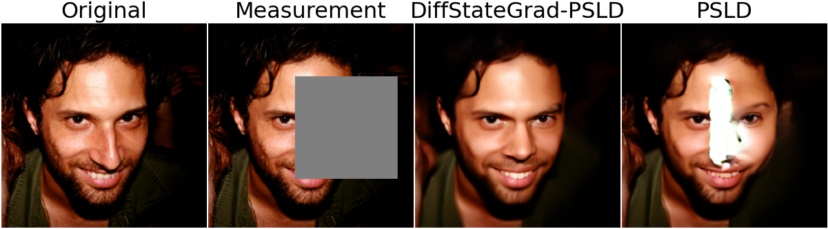
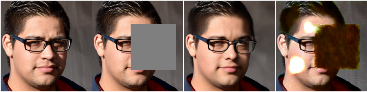
(a) Box inpainting.

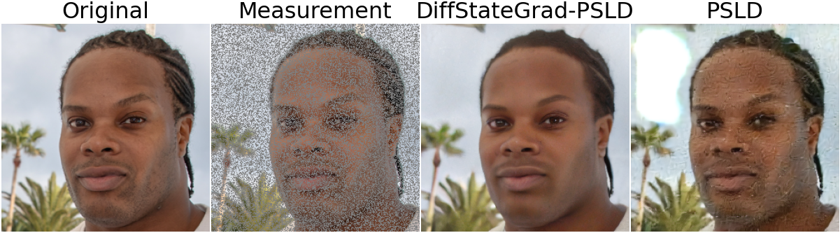
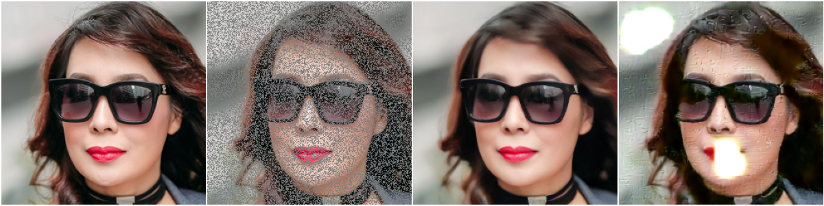
(b) Random inpainting.

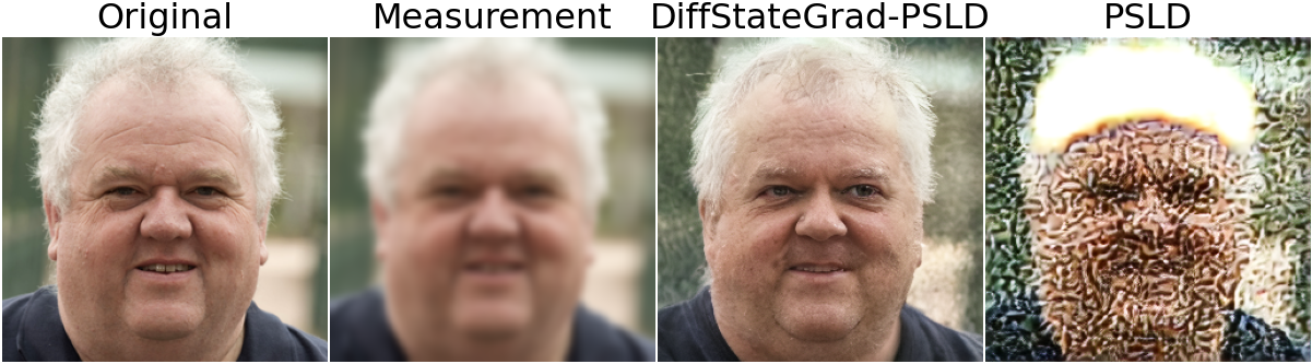
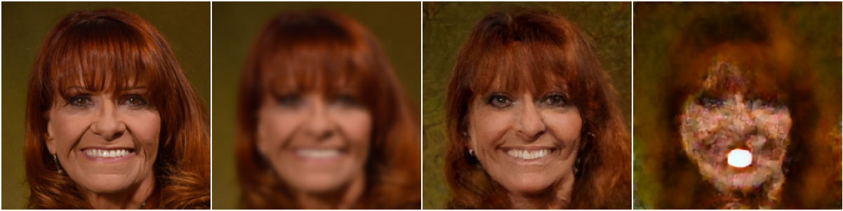
(c) Gaussian deblur.

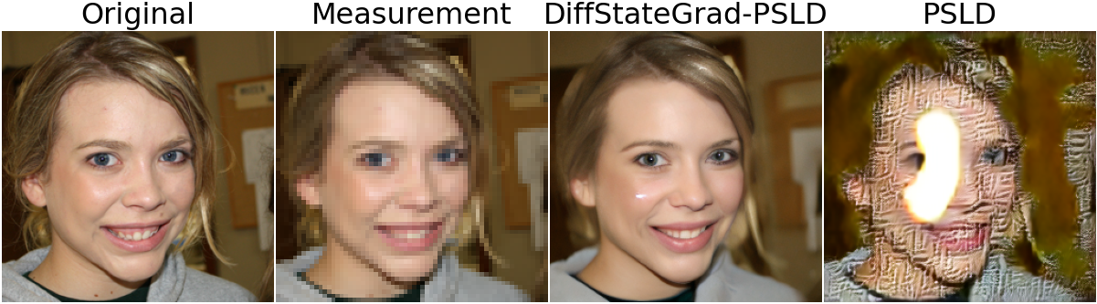
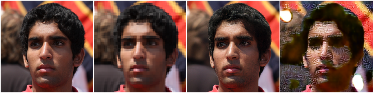
(d) Super-resolution ($\times 4$).

Figure 11: Qualitative comparison of DiffStateGrad-PSLD and PSLD for a large MG step size. Images are chosen at random for visualization.

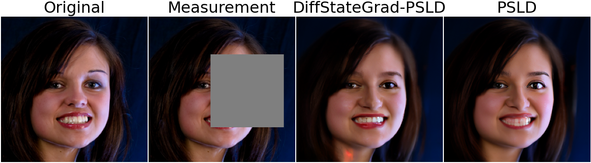
(a) Box inpainting.

(b) Random inpainting.

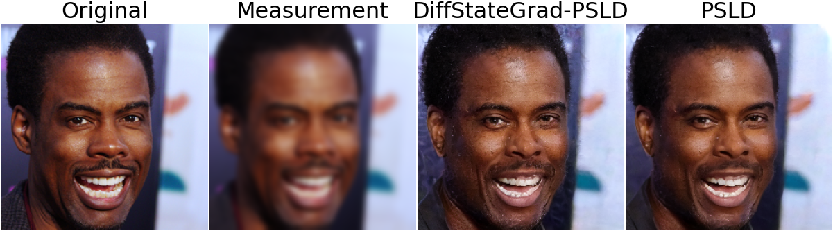
(c) Gaussian deblur.

(d) Super-resolution ($\times 4$).

Figure 12: Qualitative comparison of DiffStateGrad-PSLD and PSLD for their best-performing MG step size. Images are chosen at random for visualization.

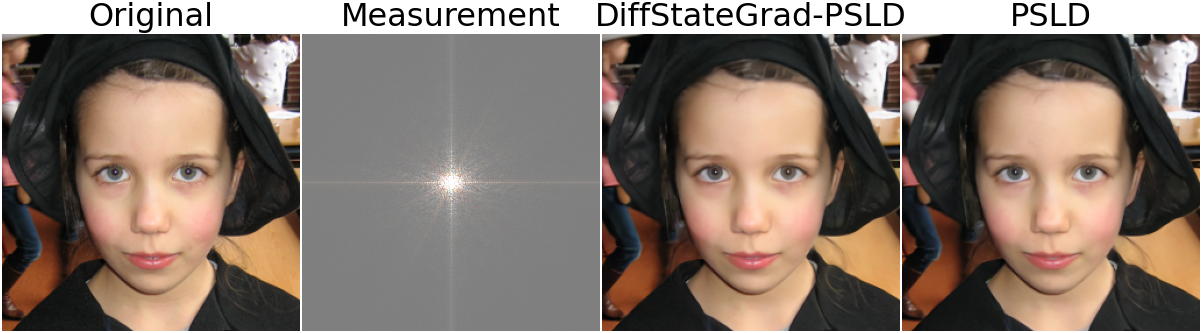
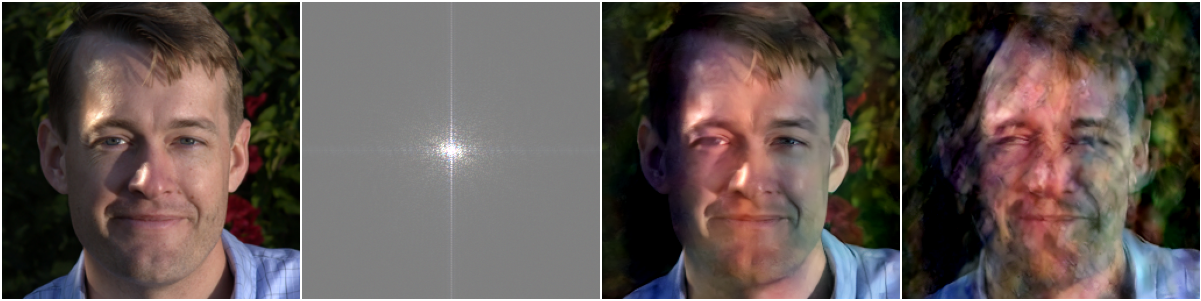
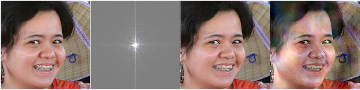
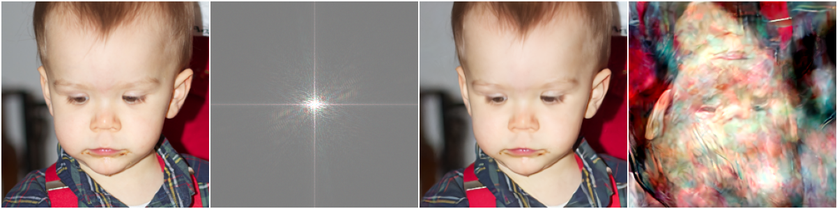
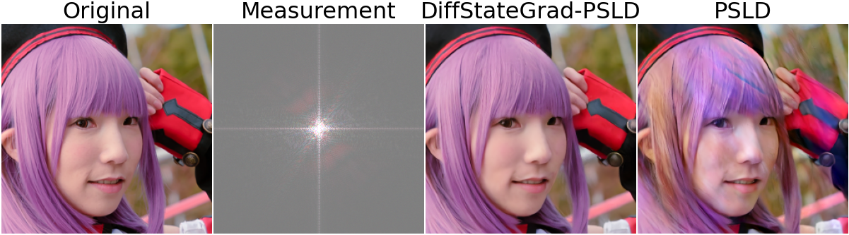
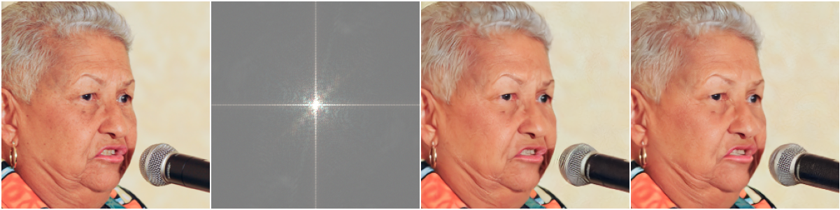
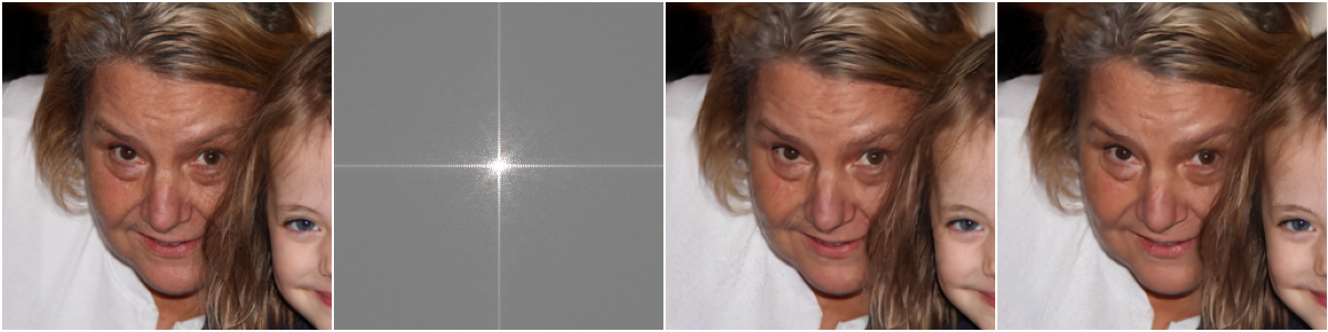
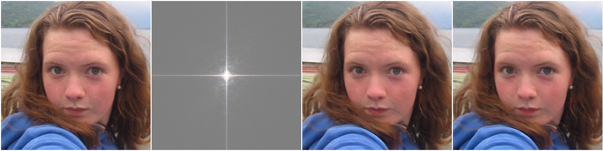
Figure 13: Qualitative comparison of DiffStateGrad-ReSample and ReSample for phase retrieval. Whereas the performance of ReSample is inconsistent, DiffStateGrad-ReSample consistently produces accurate reconstructions. Images are chosen at random for visualization.

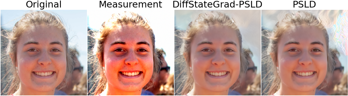
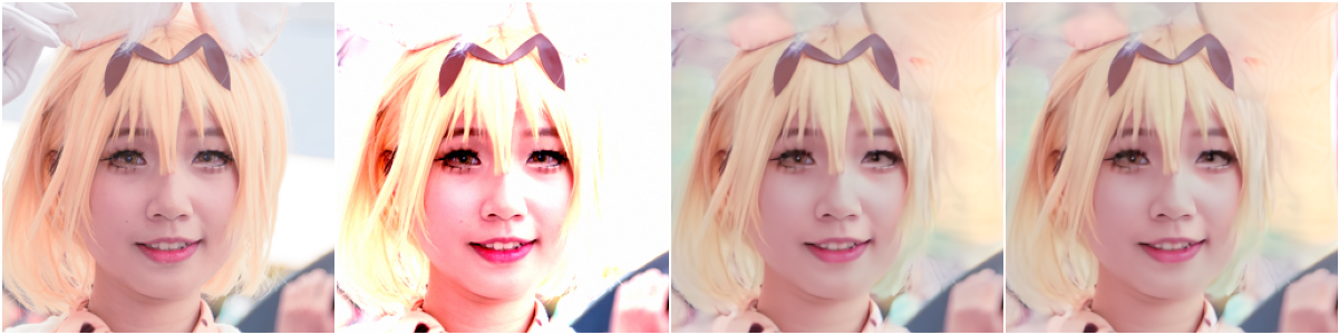
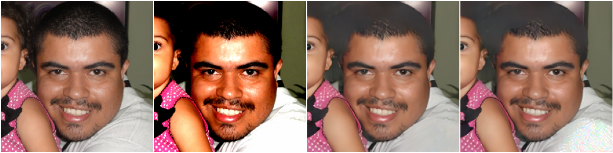
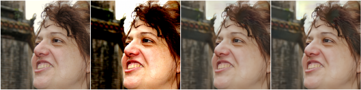
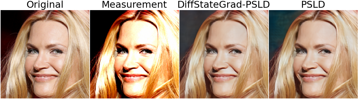
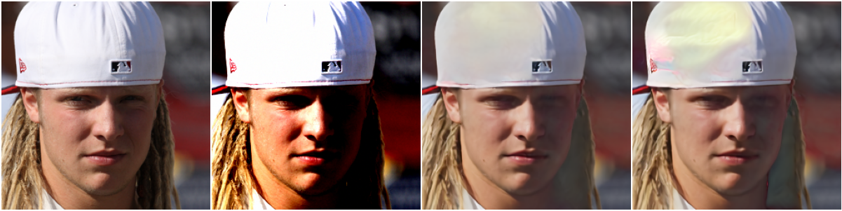
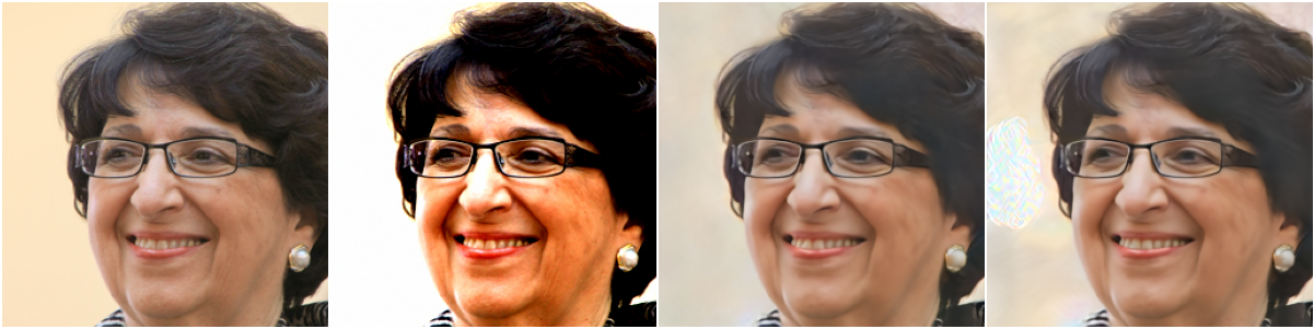
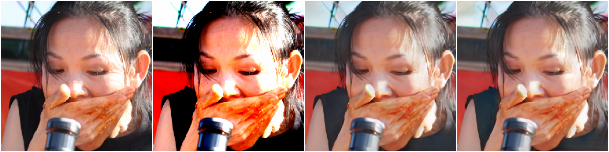
Figure 14: Qualitative comparison of DiffStateGrad-ReSample and ReSample for high dynamic range (HDR). Images are chosen at random for visualization.

Appendix C Implementation Details

C.1 Hyperparameters

For all main experiments across all three methods, we use the variance retention threshold $\tau=0.99$. For all experiments involving PSLD and DAPS, we perform the DiffStateGrad projection step every iteration ($F=1$). For all experiments involving ReSample, we perform the step every five iterations ($F=5$). See the sections dedicated to each method for further implementation details. We reiterate that various values of $\tau$ are reasonable options for optimal performance (see Figures 10 and 8).

C.2 Efficiency Experiment

We evaluate the computational overhead introduced by DiffStateGrad across three diffusion-based methods: PSLD, ReSample, and DAPS. We conduct these experiments on the box inpainting task using an NVIDIA GeForce RTX 4090 GPU with 24GB of VRAM. Each method is run with its default settings on a set of 100 images from FFHQ $256\times 256$, and we measure the average runtime in seconds per image.

C.3 PSLD

Our DiffStateGrad-PSLD algorithm integrates the state-guided projected gradient directly into the PSLD update process. For each iteration (i.e., frequency $F=1$) of the main loop, after computing the standard PSLD update ${\bm{z}}^{\prime}_{t-1}$, we introduce our DiffStateGrad method. First, we calculate the full gradient $\bm{G}_{t}$ according to PSLD, combining both the measurement consistency term and the fixed-point constraint. We then perform SVD on the current latent representation (or diffusion state) ${\bm{Z}}_{t}$ (${\bm{z}}_{t}$ in image matrix form). Using the variance retention threshold $\tau$, we determine the appropriate rank for our projection. We construct projection matrices from the truncated singular vectors and use these to approximate the gradient. This approximated gradient $\bm{G}^{\prime}_{t}$ is then used for the final update step, replacing the separate gradient updates in standard PSLD. This process is repeated at every iteration, allowing for adaptive, low-rank updates throughout the entire diffusion process.

For experiments, we use the official implementation of PSLD (Rout et al., 2023) with default configurations.

Algorithm 2 DiffStateGrad-PSLD for Image Restoration Tasks

1:$T,\bm{y},\{\eta_{t}\}_{t=1}^{T},\{\gamma_{t}\}_{t=1}^{T},\{\tilde{\sigma}_{t}\}_{t=1}^{T}$

2:$\mathcal{E},\mathcal{D},\mathcal{A}{\bm{x}}_{0}^{\ast},\mathcal{A},\bm{s}_{\theta},$variance retention threshold $\tau$

3:${\bm{z}}_{T}\sim\mathcal{N}(\bm{0},\bm{I})$

4:for $t=T-1$ to $0$ do

5:     $\hat{\bm{s}}\leftarrow\bm{s}_{\theta}({\bm{z}}_{t},t)$

6:     $\hat{{\bm{z}}}_{0}\leftarrow\frac{1}{\sqrt{\bar{\alpha_{t}}}}({\bm{z}}_{t}+(1-\bar{\alpha_{t}})\hat{\bm{s}})$

7:     $\bm{\epsilon}\sim\mathcal{N}(\bm{0},\bm{I})$

8:     ${\bm{z}}^{\prime}_{t-1}\leftarrow\frac{\sqrt{\alpha_{t}}(1-\bar{\alpha}_{t-1})}{1-\bar{\alpha}_{t}}{\bm{z}}_{t}+\frac{\sqrt{\bar{\alpha}_{t-1}}\beta_{t}}{1-\bar{\alpha}_{t}}\hat{{\bm{z}}}_{0}+\tilde{\sigma}_{t}\bm{\epsilon}$

9:     $\bm{g}_{t}\leftarrow\eta_{t}\nabla_{{\bm{z}}_{t}}\|\bm{y}-\mathcal{A}(\mathcal{D}(\hat{{\bm{z}}}_{0}))\|^{2}_{2}+\gamma_{t}\nabla_{{\bm{z}}_{t}}\|\hat{{\bm{z}}}_{0}-\mathcal{E}(\mathcal{A}^{T}\mathcal{A}{\bm{x}}_{0}^{\ast}+(\bm{I}-\mathcal{A}^{T}\mathcal{A})\mathcal{D}(\hat{{\bm{z}}}_{0}))\|^{2}_{2}$

10:     $\bm{U},\bm{S},\bm{V}\leftarrow\text{SVD}(\bm{Z}_{t})$ 

11:     $\lambda_{j}\leftarrow s_{j}^{2}$ ($s_{j}$ are the singular values of $\bm{S}$)

12:     $c_{k}\leftarrow\frac{\sum_{j=1}^{k}\lambda_{j}}{\sum_{j}\lambda_{j}}$

13:     $r\leftarrow\underset{k}{\operatorname*{arg\,min}}\{c_{k}\geq\tau\}$

14:     $\bm{A}_{t}\leftarrow\bm{U}_{r}$

15:     $\bm{B}_{t}\leftarrow\bm{V}_{r}$

16:     $\bm{R}_{t}\leftarrow\bm{A}_{t}^{T}\bm{G}_{t}\bm{B}_{t}^{T}$

17:     $\bm{G}^{\prime}_{t}\leftarrow\bm{A}_{t}\bm{R}_{t}\bm{B}_{t}$

18:     ${\bm{z}}_{t-1}\leftarrow{\bm{z}}^{\prime}_{t-1}-\bm{g}^{\prime}_{t}$

19:end for

20:return $\mathcal{D}(\hat{{\bm{z}}}_{0})$

C.4 ReSample

Our DiffStateGrad-ReSample algorithm integrates the state-guided projected gradient into the optimization process of ReSample (Song et al., 2023a). We introduce two new hyperparameters: the variance retention threshold $\tau$ and a frequency $F$ for applying our DiffStateGrad step. During each ReSample step, we first perform SVD on the current latent representation (or diffusion state) ${\bm{Z}}^{\prime}_{t}$ (${\bm{z}}^{\prime}_{t}$ in image matrix form). Note that we do not perform SVD within the gradient descent loop itself, meaning that we only perform SVD at most once per iteration of the sampling algorithm. We then determine the appropriate rank based on $\tau$ and construct projection matrices. Then, within the gradient descent loop for solving $\hat{{\bm{z}}}_{0}({\bm{y}})$, we approximate the gradient in the diffusion state subspace using our projection matrices every $F=5$ steps. On steps where DiffStateGrad is not applied, we use the standard gradient. This adaptive, periodic application of DiffStateGrad allows for a balance between the benefits of low-rank approximation and the potential need for full gradient information. The rest of the ReSample algorithm, including the stochastic resampling step, remains unchanged.

We note that the ReSample algorithm employs a two-stage approach for its hard data consistency step. Initially, it performs pixel-space optimization. This step is computationally efficient and produces smoother, albeit potentially blurrier, results with high-level semantic information. As the diffusion process approaches $t=0$, ReSample transitions to latent-space optimization to refine the image with finer details. Our DiffStateGrad method is specifically integrated into this latter, latent-space optimization stage. By applying DiffStateGrad to the latent optimization, we aim to mitigate the potential introduction of artifacts and off-manifold deviations that can occur due to the direct manipulation of latent variables. This application of DiffStateGrad allows us to benefit from the computational efficiency of initial pixel-space optimization while enhancing the robustness and quality of the final latent-space refinement. Importantly, DiffStateGrad is not applied during the pixel-space optimization phase, as this stage already tends to produce smoother results and is less prone to artifact introduction.

For experiments, we use the official implementation of ReSample (Song et al., 2023a) with default configurations.

Algorithm 3 DiffStateGrad-ReSample for Image Restoration Tasks

1:Measurements ${\bm{y}}$, $\mathcal{A}(\cdot)$, Encoder $\mathcal{E}(\cdot)$, Decoder $\mathcal{D}(\cdot)$, Score function ${\bm{s}}_{\theta}(\cdot,t)$, Pretrained LDM Parameters $\beta_{t}$, $\bar{\alpha}_{t}$, $\eta$, $\delta$, Hyperparameter $\gamma$ to control $\sigma_{t}^{2}$, Time steps to perform resample $C$, Variance retention threshold $\tau$, Frequency $F$

2:${\bm{z}}_{T}\sim\mathcal{N}(\mathbf{0},\bm{I})$ $\triangleright$ Initial noise vector

3:for $t=T-1,\ldots,0$ do

4:     $\bm{\epsilon}_{1}\sim\mathcal{N}(\mathbf{0},\bm{I})$

5:     $\hat{\bm{\epsilon}}_{t+1}={\bm{s}}_{\theta}({\bm{z}}_{t+1},t+1)$ $\triangleright$ Compute the score

6:     $\hat{{\bm{z}}}_{0}({\bm{z}}_{t+1})=\frac{1}{\sqrt{\bar{\alpha}_{t+1}}}({\bm{z}}_{t+1}-\sqrt{1-\bar{\alpha}_{t+1}}\hat{\bm{\epsilon}}_{t+1})$ $\triangleright$ Predict $\hat{{\bm{z}}}_{0}$ using Tweedie’s formula

7:     ${\bm{z}}^{\prime}_{t}=\sqrt{\bar{\alpha}_{t}}\hat{{\bm{z}}}_{0}({\bm{z}}_{t+1})+\sqrt{1-\bar{\alpha}_{t}-\eta\delta^{2}}\hat{\bm{\epsilon}}_{t+1}+\eta\delta\bm{\epsilon}_{1}$ $\triangleright$ Unconditional DDIM step

8:     if $t\in C$ then $\triangleright$ ReSample time step

9:          Initialize $\hat{{\bm{z}}}_{0}({\bm{y}})$ with $\hat{{\bm{z}}}_{0}({\bm{z}}_{t+1})$

10:          $\bm{U},\bm{S},\bm{V}\leftarrow\text{SVD}(\bm{Z}^{\prime}_{t})$ $\triangleright$ Perform SVD on current diffusion state

11:          $\lambda_{j}\leftarrow s_{j}^{2}$ (where $s_{j}$ are the singular values of $\bm{S}$) $\triangleright$ Calculate eigenvalues

12:          $c_{k}\leftarrow\frac{\sum_{j=1}^{k}\lambda_{j}}{\sum_{j}\lambda_{j}}$ $\triangleright$ Cumulative sum of eigenvalues

13:          $r\leftarrow\underset{k}{\operatorname*{arg\,min}}\{c_{k}\geq\tau\}$ $\triangleright$ Determine rank $r$ based on threshold $\tau$

14:          $\bm{A}\leftarrow\bm{U}_{r}$ $\triangleright$ Get first $r$ left singular vectors

15:          $\bm{B}\leftarrow\bm{V}_{r}$ $\triangleright$ Get first $r$ right singular vectors

16:         for  each step in gradient descent do

17:              if  step number $\mod F=0$ then

18:                   $\bm{g}\leftarrow\nabla_{\hat{{\bm{z}}}_{0}({\bm{y}})}\frac{1}{2}\|{\bm{y}}-\mathcal{A}(\mathcal{D}(\hat{{\bm{z}}}_{0}({\bm{y}})))\|_{2}^{2}$ $\triangleright$ Compute gradient

19:                   $\bm{R}\leftarrow\bm{A}^{T}\bm{G}\bm{B}^{T}$ $\triangleright$ Project gradient

20:                   $\bm{G}^{\prime}\leftarrow\bm{A}\bm{R}\bm{B}$ $\triangleright$ Reconstruct approximated gradient

21:              else

22:                   $\bm{g}^{\prime}\leftarrow\nabla_{\hat{{\bm{z}}}_{0}({\bm{y}})}\frac{1}{2}\|{\bm{y}}-\mathcal{A}(\mathcal{D}(\hat{{\bm{z}}}_{0}({\bm{y}})))\|_{2}^{2}$ $\triangleright$ Compute gradient without modification

23:              end if

24:               Update $\hat{{\bm{z}}}_{0}({\bm{y}})$ using gradient $\bm{g}^{\prime}$

25:         end for

26:         ${\bm{z}}_{t}=\text{StochasticResample}(\hat{{\bm{z}}}_{0}({\bm{y}}),{\bm{z}}^{\prime}_{t},\gamma)$ $\triangleright$ Map back to $t$

27:     else

28:         ${\bm{z}}_{t}={\bm{z}}^{\prime}_{t}$ $\triangleright$ Unconditional sampling if not resampling

29:     end if

30:end for

31:${\bm{x}}_{0}=\mathcal{D}({\bm{z}}_{0})$ $\triangleright$ Output reconstructed image

32:return ${\bm{x}}_{0}$

C.5 DAPS

We improve upon DAPS by incorporating a state-guided projected gradient. We introduce a variance retention threshold $\tau$ to determine the projection rank. For each noise level in the annealing loop, DAPS computes the initial estimate $\hat{{\bm{x}}}_{0}^{(0)}$ by solving the probability flow ODE using the score model ${\bm{s}}_{\theta}$. This estimate represents a guess of the clean image given the current noisy sample ${\bm{x}}_{t_{i}}$. We then perform SVD on this estimate in image matrix form $\hat{\bm{X}}_{0}^{(0)}$ (using it as our diffusion state), determine the appropriate rank based on $\tau$, and construct projection matrices. Within the Langevin dynamics loop, we calculate the full gradient, combining both the prior term $\log p(\hat{{\bm{x}}}_{0}^{(j)}|{\bm{x}}_{t_{i}})$ and the likelihood term $\log p({\bm{y}}|\hat{{\bm{x}}}_{0}^{(j)})$. For each step (i.e., frequency $F=1$), we project this gradient using our pre-computed matrices and use this projected gradient for the update step. This process is repeated for each noise level, progressively refining our estimate of the clean image.

For experiments, we use the official implementation of DAPS (Zhang et al., 2024) with default configurations.

Algorithm 4 DiffStateGrad-DAPS for Image Restoration Tasks

1:Score model ${\bm{s}}_{\theta}$, measurement ${\bm{y}}$, noise schedule $\sigma_{t}$, $\{t_{i}\}_{i\in\{0,\ldots,N_{A}\}}$, variance retention threshold $\tau$

2:Sample ${\bm{x}}_{T}\sim\mathcal{N}(\mathbf{0},\sigma_{T}^{2}\bm{I})$

3:for $i=N_{A},N_{A}-1,\ldots,1$ do

4:     Compute $\hat{{\bm{x}}}_{0}^{(0)}=\hat{{\bm{x}}}_{0}({\bm{x}}_{t_{i}})$ by solving the probability flow ODE in Eq. (39) with ${\bm{s}}_{\theta}$

5:      $\bm{U},\bm{S},\bm{V}\leftarrow\text{SVD}(\hat{\bm{X}}_{0}^{(0)})$ $\triangleright$ Perform SVD on initial estimate

6:      $\lambda_{j}\leftarrow s_{j}^{2}$ (where $s_{j}$ are the singular values of $\bm{S}$) $\triangleright$ Calculate eigenvalues

7:      $c_{k}\leftarrow\frac{\sum_{j=1}^{k}\lambda_{j}}{\sum_{j}\lambda_{j}}$ $\triangleright$ Cumulative sum of eigenvalues

8:      $r\leftarrow\underset{k}{\operatorname*{arg\,min}}\{c_{k}\geq\tau\}$ $\triangleright$ Determine rank $r$ based on threshold $\tau$

9:      $\bm{A}\leftarrow\bm{U}_{r}$ $\triangleright$ Get first $r$ left singular vectors

10:      $\bm{B}\leftarrow\bm{V}_{r}$ $\triangleright$ Get first $r$ right singular vectors

11:     for $j=0,\ldots,N-1$ do

12:          $\bm{g}\leftarrow\nabla_{\hat{{\bm{x}}}_{0}}\log p(\hat{{\bm{x}}}_{0}^{(j)}|{\bm{x}}_{t_{i}})+\nabla_{\hat{{\bm{x}}}_{0}}\log p({\bm{y}}|\hat{{\bm{x}}}_{0}^{(j)})$ $\triangleright$ Compute gradient

13:          $\bm{R}\leftarrow\bm{A}^{T}\bm{G}\bm{B}^{T}$ $\triangleright$ Project gradient

14:          $\bm{G}^{\prime}\leftarrow\bm{A}\bm{R}\bm{B}$ $\triangleright$ Reconstruct approximated gradient

15:         $\hat{{\bm{x}}}_{0}^{(j+1)}\leftarrow\hat{{\bm{x}}}_{0}^{(j)}+\eta_{t}\bm{g}^{\prime}+\sqrt{2\eta_{t}}\bm{\epsilon}_{j}$, $\bm{\epsilon}_{j}\sim\mathcal{N}(\mathbf{0},\bm{I})$

16:     end for

17:     Sample ${\bm{x}}_{t_{i-1}}\sim\mathcal{N}(\hat{{\bm{x}}}_{0}^{(N)},\sigma_{t_{i-1}}^{2}\bm{I})$

18:end for

19:return ${\bm{x}}_{0}$

Appendix D Proofs

See 1

Proof.

Let ${\bm{z}}_{t}\in\mathcal{M}$ and ${\bm{g}}_{t}\in\mathbb{R}^{d}$. Decompose the gradient ${\bm{g}}_{t}$ into components tangent and normal to $\mathcal{M}$ at ${\bm{z}}_{t}$:

$${\bm{g}}_{t}={\bm{g}}_{t}^{\parallel}+{\bm{g}}_{t}^{\perp},$$

where ${\bm{g}}_{t}^{\parallel}\in T_{{\bm{z}}_{t}}\mathcal{M}$ and ${\bm{g}}_{t}^{\perp}\in N_{{\bm{z}}_{t}}\mathcal{M}$, the normal space at ${\bm{z}}_{t}$.

We have two projection operators:

• $\mathcal{P}_{T_{{\bm{z}}_{t}}\mathcal{M}}$: the exact orthogonal projection onto the tangent space $T_{{\bm{z}}_{t}}\mathcal{M}$.

• $\mathcal{P}_{\mathcal{S}_{{\bm{z}}_{t}}}$: an approximate projection operator onto a subspace $\mathcal{S}_{{\bm{z}}_{t}}$ that closely approximates $T_{{\bm{z}}_{t}}\mathcal{M}$.

Assuming that $\mathcal{P}_{\mathcal{S}_{{\bm{z}}_{t}}}$ approximates $\mathcal{P}_{T_{{\bm{z}}_{t}}\mathcal{M}}$, we have:

$$\mathcal{P}_{\mathcal{S}_{{\bm{z}}_{t}}}({\bm{g}}_{t})={\bm{g}}_{t}^{\parallel}+\bm{\epsilon},$$

where $\bm{\epsilon}=\mathcal{P}_{\mathcal{S}_{{\bm{z}}_{t}}}({\bm{g}}_{t})-{\bm{g}}_{t}^{\parallel}$ is the approximation error, which is small.

The standard update is:

$${\bm{z}}_{t-1}={\bm{z}}_{t}-\eta{\bm{g}}_{t}={\bm{z}}_{t}-\eta({\bm{g}}_{t}^{\parallel}+{\bm{g}}_{t}^{\perp}).$$

The projected update is:

$${\bm{z}}_{t-1}^{\prime}={\bm{z}}_{t}-\eta\mathcal{P}_{\mathcal{S}_{{\bm{z}}_{t}}}({\bm{g}}_{t})={\bm{z}}_{t}-\eta({\bm{g}}_{t}^{\parallel}+\bm{\epsilon}).$$

Let $\pi({\bm{z}})$ denote the orthogonal projection of ${\bm{z}}$ onto $\mathcal{M}$. For points close to ${\bm{z}}_{t}$, we can approximate $\pi({\bm{z}})$ using the tangent space projection, which comes from the first-order Taylor expansion of $\mathcal{M}$ at ${\bm{z}}_{t}$:

$$\pi({\bm{z}})\approx{\bm{z}}_{t}+\mathcal{P}_{T_{{\bm{z}}_{t}}\mathcal{M}}({\bm{z}}-{\bm{z}}_{t}).$$

Here, the higher-order terms for $\pi({\bm{z}}_{t-1})$ are of order $\mathcal{O}(\|{\bm{z}}_{t-1}-{\bm{z}}_{t}\|^{2})=\mathcal{O}((\eta\|{\bm{g}}_{t}\|)^{2})=\mathcal{O}(\eta^{2})$. Similarly, the higher-order terms for $\pi({\bm{z}}_{t-1}^{\prime})$ are of order $\mathcal{O}(\|{\bm{z}}_{t-1}^{\prime}-{\bm{z}}_{t}\|^{2})=\mathcal{O}((\eta\|\mathcal{P}_{\mathcal{S}_{{\bm{z}}_{t}}}({\bm{g}}_{t})\|)^{2})=\mathcal{O}(\eta^{2})$. We will address these terms at the end of the proof.

First, compute the distance from ${\bm{z}}_{t-1}$ to $\mathcal{M}$:

$$\text{dist}({\bm{z}}_{t-1},\mathcal{M}) =\left\|{\bm{z}}_{t-1}-\pi({\bm{z}}_{t-1})\right\|$$

$$\approx\left\|{\bm{z}}_{t}-\eta({\bm{g}}_{t}^{\parallel}+{\bm{g}}_{t}^{\perp})-\left({\bm{z}}_{t}+\mathcal{P}_{T_{{\bm{z}}_{t}}\mathcal{M}}(-\eta({\bm{g}}_{t}^{\parallel}+{\bm{g}}_{t}^{\perp}))\right)\right\|$$

$$=\left\|-\eta({\bm{g}}_{t}^{\parallel}+{\bm{g}}_{t}^{\perp})+\eta\mathcal{P}_{T_{{\bm{z}}_{t}}\mathcal{M}}({\bm{g}}_{t}^{\parallel}+{\bm{g}}_{t}^{\perp})\right\|$$

$$=\left\|-\eta{\bm{g}}_{t}^{\perp}+\eta\mathcal{P}_{T_{{\bm{z}}_{t}}\mathcal{M}}({\bm{g}}_{t}^{\perp})\right\|$$

$$=\eta\left\|{\bm{g}}_{t}^{\perp}-\mathcal{P}_{T_{{\bm{z}}_{t}}\mathcal{M}}({\bm{g}}_{t}^{\perp})\right\|.$$

Since ${\bm{g}}_{t}^{\perp}\in N_{{\bm{z}}_{t}}\mathcal{M}$ and $\mathcal{P}_{T_{{\bm{z}}_{t}}\mathcal{M}}({\bm{g}}_{t}^{\perp})=\mathbf{0}$, we have:

$$\text{dist}({\bm{z}}_{t-1},\mathcal{M})=\eta\left\|{\bm{g}}_{t}^{\perp}\right\|.$$ (9)

Now, compute the distance from ${\bm{z}}_{t-1}^{\prime}$ to $\mathcal{M}$:

$$\text{dist}({\bm{z}}_{t-1}^{\prime},\mathcal{M}) =\left\|{\bm{z}}_{t-1}^{\prime}-\pi({\bm{z}}_{t-1}^{\prime})\right\|$$

$$\approx\left\|{\bm{z}}_{t}-\eta({\bm{g}}_{t}^{\parallel}+\bm{\epsilon})-\left({\bm{z}}_{t}+\mathcal{P}_{T_{{\bm{z}}_{t}}\mathcal{M}}(-\eta({\bm{g}}_{t}^{\parallel}+\bm{\epsilon}))\right)\right\|$$

$$=\left\|-\eta({\bm{g}}_{t}^{\parallel}+\bm{\epsilon})+\eta\mathcal{P}_{T_{{\bm{z}}_{t}}\mathcal{M}}({\bm{g}}_{t}^{\parallel}+\bm{\epsilon})\right\|$$

$$=\left\|-\eta\bm{\epsilon}+\eta\mathcal{P}_{T_{{\bm{z}}_{t}}\mathcal{M}}(\bm{\epsilon})\right\|$$

$$=\eta\left\|\bm{\epsilon}-\mathcal{P}_{T_{{\bm{z}}_{t}}\mathcal{M}}(\bm{\epsilon})\right\|$$

$$=\eta\left\|(I-\mathcal{P}_{T_{{\bm{z}}_{t}}\mathcal{M}})\bm{\epsilon}\right\|.$$

Since $\left\|\bm{\epsilon}^{\perp}\right\|=\left\|(I-\mathcal{P}_{T_{{\bm{z}}_{t}}\mathcal{M}})\bm{\epsilon}\right\|$, we have:

$$\text{dist}({\bm{z}}_{t-1}^{\prime},\mathcal{M})=\eta\left\|\bm{\epsilon}^{\perp}\right\|.$$ (10)

Because $\bm{\epsilon}$ is small, we can bound $\left\|\bm{\epsilon}^{\perp}\right\|\leq c^{\prime}\left\|{\bm{g}}_{t}^{\perp}\right\|$ for some small constant $c^{\prime}>0$.

Therefore,

$$\text{dist}({\bm{z}}_{t-1}^{\prime},\mathcal{M})\leq c^{\prime}\eta\left\|{\bm{g}}_{t}^{\perp}\right\|.$$

Comparing the distances, we have:

$$\text{dist}({\bm{z}}_{t-1},\mathcal{M})-\text{dist}({\bm{z}}_{t-1}^{\prime},\mathcal{M}) \geq\eta\left\|{\bm{g}}_{t}^{\perp}\right\|-c^{\prime}\eta\left\|{\bm{g}}_{t}^{\perp}\right\|$$

$$=(1-c^{\prime})\eta\left\|{\bm{g}}_{t}^{\perp}\right\|$$

$$=c\eta\left\|{\bm{g}}_{t}^{\perp}\right\|,$$

where $c=1-c^{\prime}>0$.

Including higher-order terms, we can write:

$$\text{dist}({\bm{z}}_{t-1}^{\prime},\mathcal{M})\leq\text{dist}({\bm{z}}_{t-1},\mathcal{M})-c\eta\left\|{\bm{g}}_{t}^{\perp}\right\|+\mathcal{O}(\eta^{2}).$$ (11)

Therefore, for sufficiently small $\eta$, the linear term dominates the higher-order terms, meaning that the projected update ${\bm{z}}_{t-1}^{\prime}$ stays closer to the manifold $\mathcal{M}$ than the standard update ${\bm{z}}_{t-1}$:

$$\text{dist}({\bm{z}}_{t-1}^{\prime},\mathcal{M})<\text{dist}({\bm{z}}_{t-1},\mathcal{M}).$$

∎

References

- Bora et al. (2017) Ashish Bora, Ajil Jalal, Eric Price, and Alexandros G Dimakis. Compressed Sensing using Generative Models. In International conference on machine learning, pp. 537–546. PMLR, 2017.
- Candès et al. (2006) Emmanuel J Candès, Justin Romberg, and Terence Tao. Robust Uncertainty Principles: Exact Signal Reconstruction from Highly Incomplete Frequency Information. IEEE Transactions on information theory, 52(2):489–509, 2006.
- Chung et al. (2022) Hyungjin Chung, Byeongsu Sim, Dohoon Ryu, and Jong Chul Ye. Improving Diffusion Models for Inverse Problems using Manifold Constraints. Advances in Neural Information Processing Systems, 35:25683–25696, 2022.
- Chung et al. (2023) Hyungjin Chung, Jeongsol Kim, Michael Thompson Mccann, Marc Louis Klasky, and Jong Chul Ye. Diffusion Posterior Sampling for General Noisy Inverse Problems. In The Eleventh International Conference on Learning Representations, 2023. URL https://openreview.net/forum?id=OnD9zGAGT0k.
- Chung et al. (2024) Hyungjin Chung, Jeongsol Kim, and Jong Chul Ye. Direct diffusion bridge using data consistency for inverse problems. Advances in Neural Information Processing Systems, 36, 2024.
- Deng et al. (2009) Jia Deng, Wei Dong, Richard Socher, Li-Jia Li, Kai Li, and Li Fei-Fei. ImageNet: A Large-Scale Hierarchical Image Database. In 2009 IEEE Conference on Computer Vision and Pattern Recognition, pp. 248–255. IEEE, 2009.
- Dhariwal & Nichol (2021) Prafulla Dhariwal and Alexander Quinn Nichol. Diffusion Models Beat GANs on Image Synthesis. In A. Beygelzimer, Y. Dauphin, P. Liang, and J. Wortman Vaughan (eds.), Advances in Neural Information Processing Systems. Curran Associates, Inc., 2021.
- Donoho (2006) David L Donoho. Compressed Sensing. IEEE Transactions on information theory, 52(4):1289–1306, 2006.
- Feng et al. (2024) Berthy T Feng, Katherine L Bouman, and William T Freeman. Event-horizon-scale imaging of m87* under different assumptions via deep generative image priors. arXiv preprint arXiv:2406.02785, 2024.
- Goodfellow et al. (2014) Ian Goodfellow, Jean Pouget-Abadie, Mehdi Mirza, Bing Xu, David Warde-Farley, Sherjil Ozair, Aaron Courville, and Yoshua Bengio. Generative Adversarial Nets. Advances in neural information processing systems, 27, 2014.
- Groetsch & Groetsch (1993) Charles W Groetsch and CW Groetsch. Inverse problems in the mathematical sciences, volume 52. Springer, 1993.
- He et al. (2024) Yutong He, Naoki Murata, Chieh-Hsin Lai, Yuhta Takida, Toshimitsu Uesaka, Dongjun Kim, Wei-Hsiang Liao, Yuki Mitsufuji, J Zico Kolter, Ruslan Salakhutdinov, et al. Manifold preserving guided diffusion. In The Twelfth International Conference on Learning Representations, 2024.
- Kadkhodaie & Simoncelli (2021) Zahra Kadkhodaie and Eero Simoncelli. Stochastic solutions for linear inverse problems using the prior implicit in a denoiser. Advances in Neural Information Processing Systems, 34:13242–13254, 2021.
- Karras et al. (2021) Tero Karras, Samuli Laine, and Timo Aila. A Style-Based Generator Architecture for Generative Adversarial Networks. IEEE Transactions on Pattern Analysis & Machine Intelligence, 43(12):4217–4228, Dec 2021.
- Kawar et al. (2022) Bahjat Kawar, Michael Elad, Stefano Ermon, and Jiaming Song. Denoising diffusion restoration models. Advances in Neural Information Processing Systems, 35:23593–23606, 2022.
- Kingma (2013) Diederik P Kingma. Auto-encoding Variational Bayes. arXiv preprint arXiv:1312.6114, 2013.
- Liu et al. (2023) Guan-Horng Liu, Arash Vahdat, De-An Huang, Evangelos Theodorou, Weili Nie, and Anima Anandkumar. I2sb: Image-to-image schrödinger bridge. In International Conference on Machine Learning, pp. 22042–22062. PMLR, 2023.
- Lustig et al. (2007) Michael Lustig, David Donoho, and John M Pauly. Sparse mri: The application of compressed sensing for rapid mr imaging. Magnetic Resonance in Medicine: An Official Journal of the International Society for Magnetic Resonance in Medicine, 58(6):1182–1195, 2007.
- Olshausen & Field (1997) Bruno A Olshausen and David J Field. Sparse coding with an overcomplete basis set: A strategy employed by v1? Vision research, 37(23):3311–3325, 1997.
- Peng et al. (2024) Xinyu Peng, Ziyang Zheng, Wenrui Dai, Nuoqian Xiao, Chenglin Li, Junni Zou, and Hongkai Xiong. Improving diffusion models for inverse problems using optimal posterior covariance. In Forty-first International Conference on Machine Learning, 2024.
- Romano et al. (2017) Yaniv Romano, Michael Elad, and Peyman Milanfar. The little engine that could: Regularization by denoising (red). SIAM Journal on Imaging Sciences, 10(4):1804–1844, 2017.
- Rombach et al. (2022) Robin Rombach, Andreas Blattmann, Dominik Lorenz, Patrick Esser, and Björn Ommer. High-resolution Image Synthesis with Latent Diffusion Models. In Proceedings of the IEEE/CVF conference on computer vision and pattern recognition, pp. 10684–10695, 2022.
- Rout et al. (2023) Litu Rout, Negin Raoof, Giannis Daras, Constantine Caramanis, Alex Dimakis, and Sanjay Shakkottai. Solving Linear Inverse Problems Provably via Posterior Sampling with Latent Diffusion Models. In Thirty-seventh Conference on Neural Information Processing Systems, 2023. URL https://openreview.net/forum?id=XKBFdYwfRo.
- Rout et al. (2024) Litu Rout, Yujia Chen, Abhishek Kumar, Constantine Caramanis, Sanjay Shakkottai, and Wen-Sheng Chu. Beyond first-order tweedie: Solving inverse problems using latent diffusion. In Proceedings of the IEEE/CVF Conference on Computer Vision and Pattern Recognition, pp. 9472–9481, 2024.
- Saharia et al. (2022) Chitwan Saharia, William Chan, Huiwen Chang, Chris Lee, Jonathan Ho, Tim Salimans, David Fleet, and Mohammad Norouzi. Palette: Image-to-image diffusion models. In ACM SIGGRAPH 2022 conference proceedings, pp. 1–10, 2022.
- Shmakov et al. (2024) Alexander Shmakov, Kevin Greif, Michael Fenton, Aishik Ghosh, Pierre Baldi, and Daniel Whiteson. End-to-end latent variational diffusion models for inverse problems in high energy physics. Advances in Neural Information Processing Systems, 36, 2024.
- Shu et al. (2023) Dule Shu, Zijie Li, and Amir Barati Farimani. A Physics-informed Diffusion Model for High-fidelity Flow Field Reconstruction. Journal of Computational Physics, 478:111972, 2023.
- Song et al. (2023a) Bowen Song, Soo Min Kwon, Zecheng Zhang, Xinyu Hu, Qing Qu, and Liyue Shen. Solving Inverse Problems with Latent Diffusion Models via Hard Data Consistency. In Conference on Parsimony and Learning (Recent Spotlight Track), 2023a. URL https://openreview.net/forum?id=iHcarDCZLn.
- Song et al. (2023b) Jiaming Song, Arash Vahdat, Morteza Mardani, and Jan Kautz. Pseudoinverse-Guided Diffusion Models for Inverse Problems. In International Conference on Learning Representations, 2023b. URL https://openreview.net/forum?id=9_gsMA8MRKQ.
- Song & Ermon (2019) Yang Song and Stefano Ermon. Generative Modeling by Estimating Gradients of the Data Distribution. In Advances in Neural Information Processing Systems, volume 32, 2019.
- Song et al. (2021) Yang Song, Jascha Sohl-Dickstein, Diederik Kingma, Abhishek Kumar, Stefano Ermon, and Ben Poole. Score-based Generative Modeling through Stochastic Differential Equations. In The International Conference on Learning Representations, 2021. URL https://openreview.net/pdf/ef0eadbe07115b0853e964f17aa09d811cd490f1.pdf.
- Stuart (2010) Andrew M Stuart. Inverse problems: a bayesian perspective. Acta numerica, 19:451–559, 2010.
- Tran et al. (2021) Phong Tran, Anh Tran, Quynh Phung, and Minh Hoai. Explore Image Deblurring via Encoded Blur Kernel Space. In Proceedings of the IEEE/CVF Conference on Computer Vision and Pattern Recognition (CVPR). IEEE, 2021.
- Ulyanov et al. (2018) Dmitry Ulyanov, Andrea Vedaldi, and Victor Lempitsky. Deep Image Prior. In Proceedings of the IEEE conference on computer vision and pattern recognition, pp. 9446–9454, 2018.
- Venkatakrishnan et al. (2013) Singanallur V Venkatakrishnan, Charles A Bouman, and Brendt Wohlberg. Plug-and-play priors for model based reconstruction. In 2013 IEEE global conference on signal and information processing, pp. 945–948. IEEE, 2013.
- Vincent (2011) Pascal Vincent. A Connection Between Score Matching and Denoising Autoencoders. Neural Computation, 23(7):1661–1674, 2011. doi: 10.1162/NECO_a_00142.
- Wang et al. (2004) Zhou Wang, Alan C Bovik, Hamid R Sheikh, and Eero P Simoncelli. Image quality assessment: from error visibility to structural similarity. IEEE transactions on image processing, 13(4):600–612, 2004.
- Wu et al. (2024) Zihui Wu, Yu Sun, Yifan Chen, Bingliang Zhang, Yisong Yue, and Katherine L Bouman. Principled probabilistic imaging using diffusion models as plug-and-play priors. arXiv preprint arXiv:2405.18782, 2024.
- Zhang et al. (2024) Bingliang Zhang, Wenda Chu, Julius Berner, Chenlin Meng, Anima Anandkumar, and Yang Song. Improving Diffusion Inverse Problem Solving with Decoupled Noise Annealing. arXiv preprint arXiv:2407.01521, 2024.
- Zhao et al. (2024) Jiawei Zhao, Zhenyu Zhang, Beidi Chen, Zhangyang Wang, Anima Anandkumar, and Yuandong Tian. Galore: Memory-efficient llm training by gradient low-rank projection. In Forty-first International Conference on Machine Learning, 2024.