Cayley Graph Propagation

Abstract

In spite of the plethora of success stories with graph neural networks (GNNs) on modelling graph-structured data, they are notoriously vulnerable to over-squashing, whereby tasks necessitate the mixing of information between distance pairs of nodes. To address this problem, prior work suggests rewiring the graph structure to improve information flow. Alternatively, a significant body of research has dedicated itself to discovering and precomputing bottleneck-free graph structures to ameliorate over-squashing. One well regarded family of bottleneck-free graphs within the mathematical community are expander graphs, with prior work—Expander Graph Propagation (EGP)—proposing the use of a well-known expander graph family—the Cayley graphs of the $\mathrm{SL}(2,\mathbb{Z}_{n})$ special linear group—as a computational template for GNNs. However, in EGP the computational graphs used are truncated to align with a given input graph. In this work, we show that truncation is detrimental to the coveted expansion properties. Instead, we propose CGP, a method to propagate information over a complete Cayley graph structure, thereby ensuring it is bottleneck-free to better alleviate over-squashing. Our empirical evidence across several real-world datasets not only shows that CGP recovers significant improvements as compared to EGP, but it is also akin to or outperforms computationally complex graph rewiring techniques.

Graph neural networks (GNNs) have emerged as a cornerstone for processing graph-structured data [1] with significant contributions in various domains and real-world applications [2, 3]. Nearly all GNNs are dependent on propagating information between neighbouring nodes in the graph [4], whereby the message-passing paradigm [5] serves as an architecture for facilitating this information. This paradigm involves the iterative exchange of messages, with nodes aggregating and updating their representations based on received information from neighbours. However, a phenomenon known as over-squashing [6] can limit the effectiveness of this message-passing process. Over-squashing occurs when a large volume of messages are aggregated into fixed-size vectors, which hinders the expressive power of GNNs, especially when dealing with long-range node interactions [7]. Consequently, the input graph’s topology is a key contributing factor to the over-squashing problem.

For this reason, the over-squashing phenomenon is an active area of research with several techniques proposed to mitigate over-squashing. Several recent works have analysed it through varying lenses, including curvature [8], spectral expansion properties [9, 10] and effective resistance [11, 12]. The majority of solutions to this problem fall under the category of graph rewiring, in which the graph topology is directly modified based on an optimisation target. However, this imposes the computational complexity of having to surgically analyse the graph structure. Notably, Expander Graph Propagation (EGP) [13] propose a unique solution of constructing an independent desirable graph structure to propagate information over.

Moreover, in the EGP paper the authors identified desirable criteria to mitigate over-squashing and effectively handle global context in graph representation learning: global information propagation (i), no bottlenecks (ii), subquadratic time and space complexity (iii) and no dedicated preprocessing (iv). The authors surveyed prior approaches, including traditional GNNs (iii, iv), master-node methods (i, iii, iv) [5, 14], fully connected graphs (i, ii, iv) [6] and the aforementioned graph rewiring techniques (i-iii), ultimately recognising the efficacy of expander graphs [15, 16] as the desirable graph structure for bottleneck-free information propagation.

In the EGP paper, a family of expander graphs have been constructed leveraging the well-known theoretical results of special linear groups, for which a family of corresponding Cayley graphs can be derived. This family of Cayley graphs is guaranteed to have the desirable expansion properties and are precomutable (i-iv). Importantly, although Cayley graphs are scalable, achieving a specific number of nodes is not always feasible; for instance, the number of nodes for a group of $n$ is known to be $O(|V|^{3})$. This consideration is addressed within the paper by identifying the smallest $n$ that yields a graph larger or equal to the desired number of nodes, and then subsequently truncating the Cayley graph to match the input graph’s number of nodes in breadth-first order.

Motivated by the promising research direction of Deac et al. [13] in which the authors use an independent graph structure that is theoretically known to exhibit desirable properties we propose a different approach of using the Cayley graph. We propose a more optimal approach of embracing the complete Cayley graph structure, guaranteeing the coveted expansion properties.

Main contributions and outline

In this paper, we present Cayley Graph Propagation (CGP), a novel model that uses the complete Cayley graph structure, which is still decoupled from the input graph’s topology, fulfilling the desirable criteria as set by EGP (i-iv). Our contributions are as follows:

• In Section 3, we highlight the theoretical benefits of using Cayley graphs for message propagation. We show that the truncation procedure performed in EGP to align the Cayley graph with the input graph may be detrimental to the coveted theoretical benefits.

• In Section 4, we introduce CGP, a method to propagate information over the complete Cayley graph structure, thereby ensuring it is bottleneck-free and alleviates over-squashing. CGP modifies EGP by avoiding the truncation step used to align the input graph with a Cayley graph, utilising the additional nodes as virtual nodes.

• In Section 5, we provide an empirical evaluation across several real-world datasets to show that CGP recovers significant improvements as compared to EGP. Additionally, our model is akin to or outperforms the computationally complex graph rewiring techniques.

Figure 1: Both Cayley graphs represent $\mathrm{SL}(2,\mathbb{Z}_{3})$ with $|V|=24$ nodes using the same construction. Left: A truncated Cayley graph (spectral gap: 0.0751, diameter: 10) aligned to a given input graph. Right: The complete Cayley graph (spectral gap: 1.2679, diameter: 4) structure indicating the additional virtual nodes (in green).

1 Background

Graph preliminaries

Given an undirected graph denoted as $G=(V,E)$, where $V$ and $E$ denote its nodes and edges respectively. The topology of the graph is encoded in the adjacency matrix ${\bf A}\in\mathbb{R}^{|n|\times|n|}$, where the number of nodes $n=|V|$. Let ${\bf D}={\bf D}(G)$ denote the diagonal matrix of degrees as given by ${\bf D}_{vv}=d_{v}$. The normalised graph Laplacian ${\bf L}={\bf L}(G)$ is defined by ${\bf L}={\bf D}^{-1/2}({\bf D}-{\bf A}){\bf D}^{-1/2}$. From the normalised Laplacian $L$ the eigenvalues $0=\lambda_{0}\leq\lambda_{1}\leq...\leq\lambda_{n-2}\leq\lambda_{n-1}$. Importantly, from this derivation the spectral gap of graph $G$ is $\lambda_{1}-\lambda_{0}=\lambda_{1}$; the Cheeger inequality then defines that a larger spectral gap of graph $G$ is an indicator of good spectral expansion properties. Accordingly, a graph with desirable expansion properties (or a larger spectral gap) defines that it has strong connectivity, or alternatively it is globally lacking bottlenecks [13].

Expander graphs

An expander graph is categorised by its unique properties of being both sparse and highly connected with the number of edges scaling linearly with the number of nodes $(|E|=O(|V|))$. One such expansion property that an expander graph satisfies is derived from the aforementioned Cheeger inequality. As a result, in essence, expander graphs do not have any bottlenecks [10]; in Section 3 we further define and explore this link.

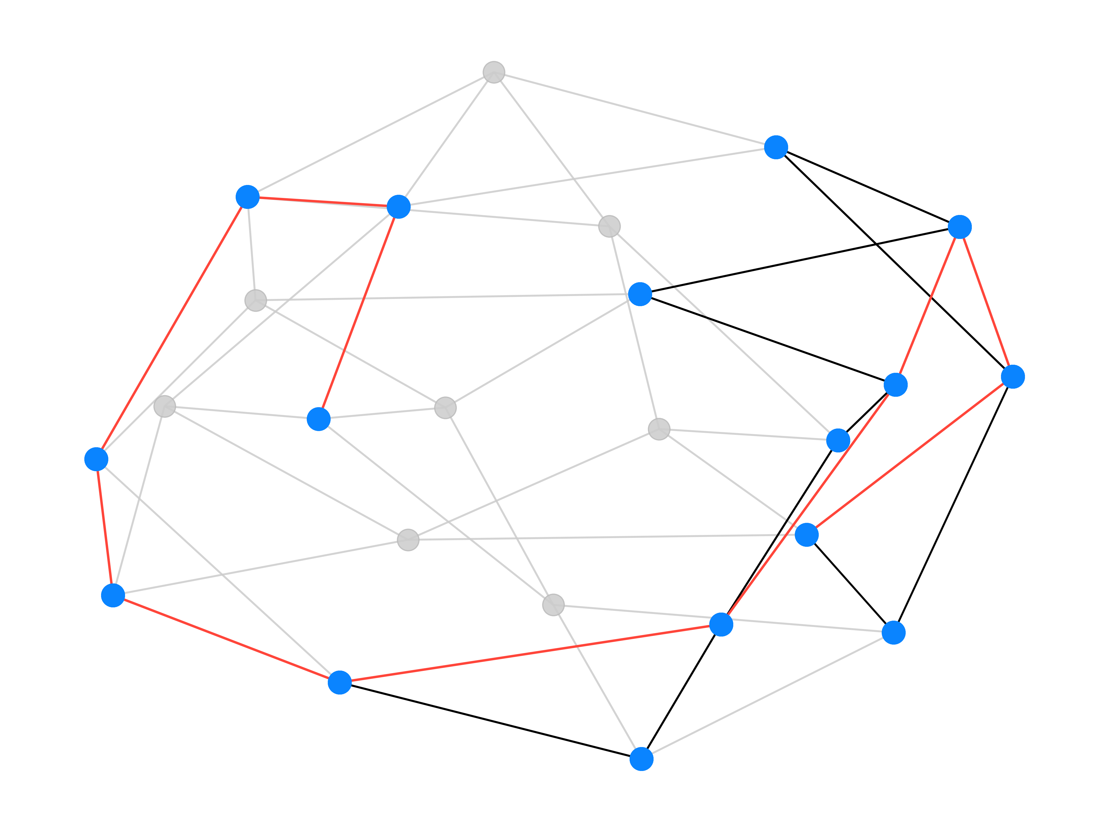
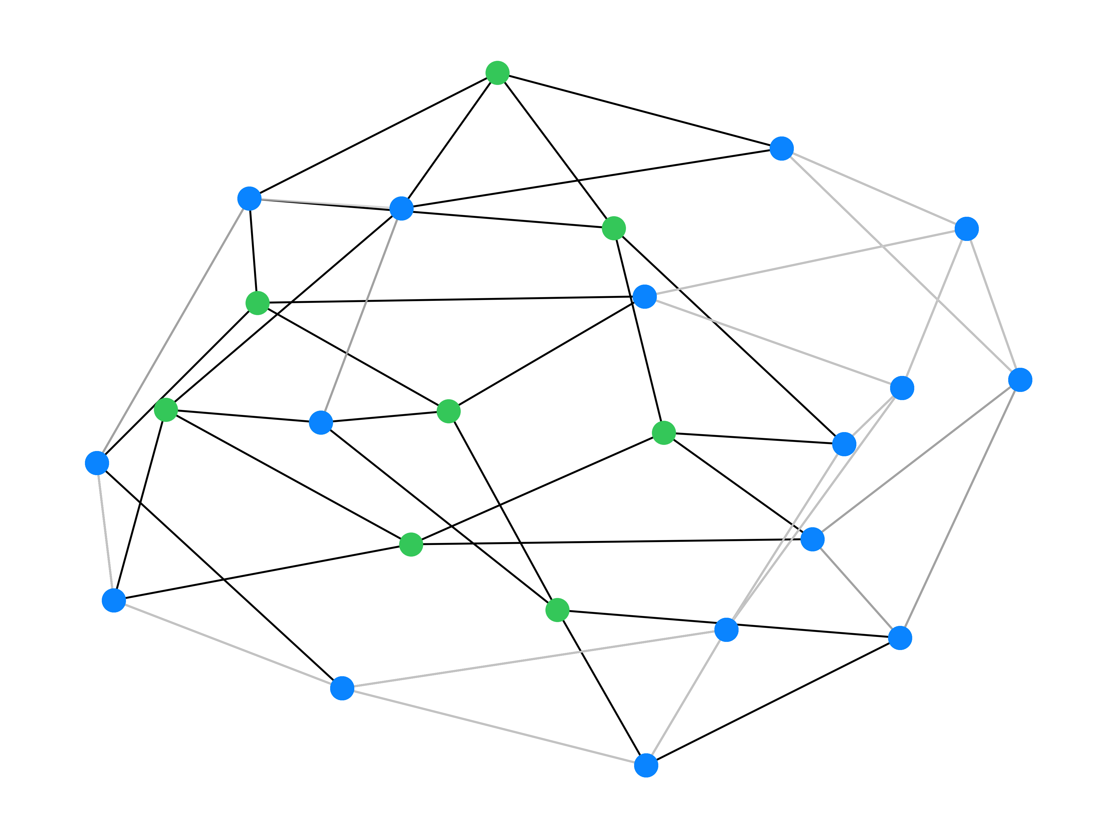
Due to the definition of an expander graph, there are consequently several known construction approaches [17, 18]. We will focus on the deterministic algebraic approach as introduced in EGP [13]. A family of expander graphs have been precomputed leveraging the well-known theoretical results of special linear groups, $\mathrm{SL}(2,\mathbb{Z}_{n})$, for which a family of corresponding Cayley graphs, $\mathrm{Cay}(\mathrm{SL}(2,\mathbb{Z}_{n});S_{n})$, can be derived. Here, $S_{n}$ ([13], Definition 8) denotes a particular generating set for $\mathrm{SL}(2,\mathbb{Z}_{n})$. For appropriate choices of $S_{n}$, the corresponding Cayley graphs are guaranteed to have expansion properties. Moreover, from Figure 1 we see that the constructed graph are 4-regular, $(|E|=2|V|)$. Importantly, although Cayley graphs are scalable, achieving a specific number of nodes is not always feasible; for instance, the node count of $\mathrm{Cay}(\mathrm{SL}(2,\mathbb{Z}_{n});S_{n})$ is given as per:

$$\left|V(\mathrm{Cay}(\mathrm{SL}(2,\mathbb{Z}_{n});S_{n}))\right|=n^{3}\prod_{\text{prime }p|n}\left(1-\frac{1}{p^{2}}\right).$$ (1)

Over-squashing

The over-squashing problem was first identified by Alon and Yahav [6], whereby the information in a MPNN is aggregated from too many neighbours, meaning as a consequence they are squashed into fixed-size vectors. This can result in a loss of information [19]. This phenomenon was then formalised [8, 11, 20], showing that the Jacobian of the node features is affected by topological properties of the graph, such as curvature and effective resistance. Furthermore, Di Giovanni et al. [7] analysed how over-squashing impacts the expressive power of GNNs. In the following section, we will address the literature and how current approaches aim to mitigate over-squashing.

Over-smoothing

Independent from over-squashing, but another well-known problem impacting the expressivity of GNNs is over-smoothing [21, 22]. This phenomenon occurs in GNNs when the number of layers increases [23, 24], such that node features become increasingly similar [25]. However, the over-smoothing problem is correlated with over-squashing due to a common approach to the latter being graph rewiring; too many additional edges lead to over-smoothing [9]. There are varying approaches to measure over-smoothing for a graph with one such notable metric being the Dirichlet energy [26, 9, 12].

2 Existing approaches to mitigate over-squashing

In this part, we explore the current landscape of several novel techniques that try to alleviate the over-squashing phenomenon [6]. In essence, the main principle behind many of these techniques is to decouple the input graph $G$ from the computational one, such that it has structurally fewer bottlenecks. Alon and Yahav [6] simply proposed a rewiring technique that does not require the analysis of the input graph by making the last layer of the GNN fully adjacent (FA), allowing all nodes to interact with each other. The effectiveness of such an approach can be shown by Graph Transformers [27, 28], where every layer is fully-connected. However, such an approach is limited by even modest graph sizes due to it imposing $O(|V|^{2})$ edges. An alternative approach is a master node [5]; here a new node is introduced, which is connected to all of the nodes within the graph. This approach is effective as it reduces the graph’s diameter to $2$ by only adding one new node with $O(|V|)$ edges. However, the master node itself becomes the bottleneck. Notably, both of the aforementioned approaches are independent in relation to the input graph topology, therefore satisfying (iv) of no dedicated preprocessing. Conversely, an approach towards this phenomenon is graph rewiring techniques [9, 12, 8], in which the input graph’s connectivity is altered in accordance with an optimisation goal.

Graph rewiring

Even though Alon and Yahav [6] were the first to introduce the over-squashing phenomenon, a plethora of research has formalised this problem [8, 10, 20]. To this end, an abundance of graph rewiring techniques have stemmed to modify the graph connectivity to try and mitigate bottlenecks. A popular class of approaches are based on a spectral quantity of a graph [9] or to reduce the effective resistance [12, 10, 11]. These approaches have provided promising insights and have empirically reduced over-squashing, but they impose a computational complexity of having to examine the input graph structure.

Expander graph based rewiring

The existing approaches of quantitative analysis leads to an alternative approach being the understanding of the desirable graph structure known as an expander graph. An expander graph exhibits the desirable properties associated with spectral gap and effective resistance. For this reason, Banerjee et al. [10] proposes a construction inspired by an expander graph to randomly locally rewire a given input graph, whilst Shirzad et al. [29] use both virtual global nodes and expander graphs as a powerful primitive to design a more scalable graph transformer architecture. As previously examined, the work of Deac et al. [13] proposes a different schema of precomputing a bank of expander graphs, which are then interwoven by alternating layers on the input graph and then the auxiliary expander layer. This schema has proven to also be successful in high-order structures [30] and in the first rewiring approach on temporal graphs [31].

3 Benefits of Cayley graphs

Figure 2: Illustrates the correlation between the Cheeger constant (left) and diameter (right) from truncated Cayley graphs of $\mathrm{SL}(2,\mathbb{Z}_{n})$. The dotted red-line represent complete Cayley graph structure for the groups of $\mathbb{Z}_{n}.$

In this section, we further explore the benefits of using Cayley graphs and why they have been used as a conduit in a number of over-squashing approaches [10, 29, 13]. In particular, we explore the implications of the expansion properties in regards to the truncated Cayley graphs used by Deac et al. [13]. In contrast to this, we examine the benefits of using the complete and regular Cayley graph structure through the lens of overfitting as per the recent work of Bechler-Speicher et al. [32].

3.1 Cayley graphs expansion properties

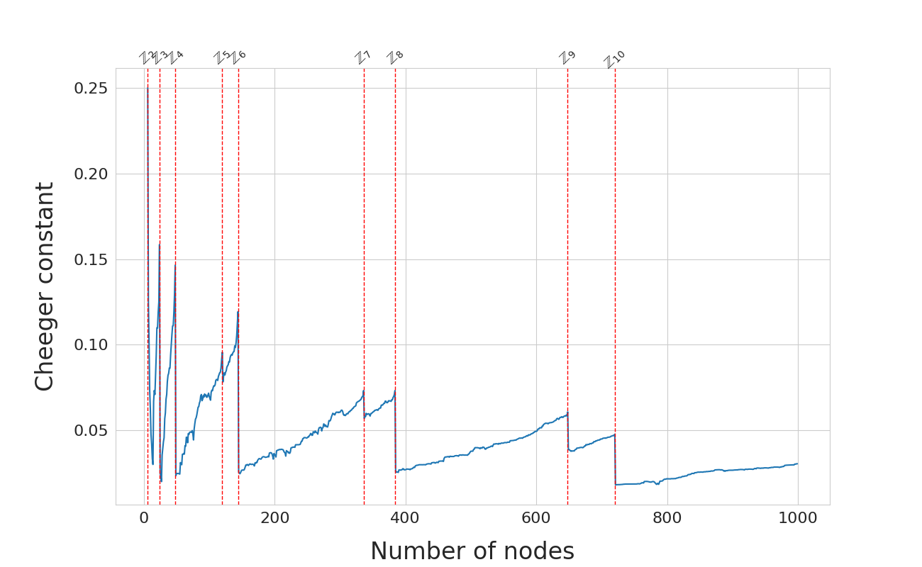
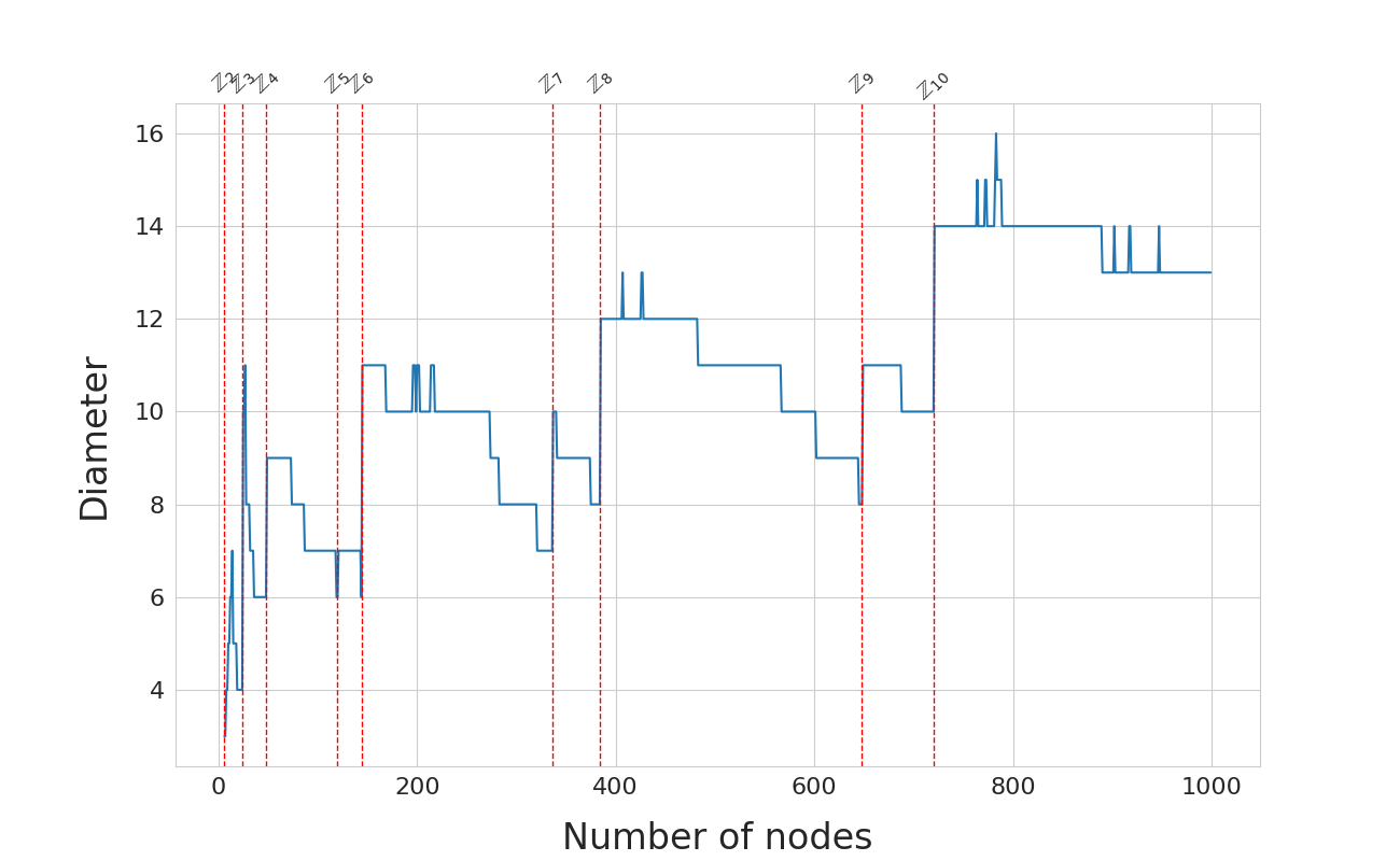
The structure of a Cayley graph makes it an ideal conduit for the propagation of information due to its sparsity and being highly connected. In particular, the family of Cayley graphs derived from $\mathrm{Cay}(\mathrm{SL}(2,\mathbb{Z}_{n});S_{n})$ are in the magnitude of $O(|V|^{3})$, and are well-known to have a high spectral gap. As from Section 1, a higher spectral gap is a desirable expansion property, meaning that it is highly connected. Correspondingly, we conjecture that truncating a Cayley graph to match an input graph as done by Deac et al. [13] will have an adverse impact on the desired expansion properties. In Figure 2 we empirically measure this impact using the Cheeger constant, as well as in respect to the diameter. In Appendix (Section D) we extend this analysis through the perspective of effective resistance, which provides a different approach to quantify over-squashing.

In the pursuit of this, the recent work of Sterner et al. [33] proposes to heuristically align the Cayley graph, such that it better aligns the corresponding edges. However, this distils to a NP-hard problem, so they opt to implement a greedy strategy to align both graphs. This method imposes a costly preprocessing time which does not comply with our desiderata (i-iv). Consequently, we do not pursue this approach further, but this variant could present an interesting avenue for future work.

Connectivity

One metric to measure a graph’s connectivity is the coveted Cheeger constant [34]. It provides a measurement of the narrowest bottleneck in a graph; a higher Cheeger constant indicates that a graph is globally lacking bottlenecks. Alternatively, it effectively describes how difficult it is to separate a graph $G$ into two subgraphs by removing edges. The exact Cheeger constant $h(G)$ is known to be a computationally challenging problem. To address this difficulty, we recall the spectral gap of a graph $G$ (defined in Section 1), which provides a bound for the Cheeger constant from discrete Cheeger inequality [35, 36]. As per Chung and Graham [34], this bound is:

$$\frac{\lambda_{1}}{2}\leq h(G)\leq\sqrt{2\lambda_{1}},$$ (2)

where $\lambda_{1}$ is the second-smallest eigenvalue or spectral gap of the normalised graph Laplacian ${\bf L}(G)$. In Figure 2, we use the lower bound from the Cheeger constant; the figure illustrates that the complete Cayley graph structure exhibits the most desirable Cheeger constant (or higher spectral gap). In turn, it is observed that the most unfavourable scenario occurs for a truncated Cayley graph just beyond the range of the proceeding graph, as derived from the special linear group $\mathrm{SL}(2,\mathbb{Z}_{n})$.

Diameter

The diameter of a graph influences the effectiveness of traversal between nodes. A lower diameter facilitates a more efficient graph structure, enabling nodes to reach each other in a shorter number of hops. Our constructed Cayley graph with $|V|$ nodes has a low diameter, requiring only $O(log(|V(G_{i})|)$ ([13], Theorem 5) steps to globally propagate information. This coincides with the work of Di Giovanni et al. [20], as they prove that over-squashing occurs between nodes with a high commute-time. Due to expander graphs having a low diameter, any node within the graph can reach another node in a short number of hops. The results in Figure 2 in relation to the diameter correlate with those shown for the Cheeger constant; the lower diameter is at each complete Cayley graph structure.

Figure 3: The learning curves of the same GNN model trained on graphs that have the same node features and only differ in their graph structure, which is sampled from different distributions. The label is computed from the node features without the use of any graph structure. The GNN overfits the graph structure instead of ignoring it, and therefore the model performance differ across different graph distributions. Cayley graphs exhibit the best performance, and robustness to overfitting.

3.2 Cayley Graphs as Regular Graphs

In this subsection, we highlight additional benefits of the Cayley graph.

Robustness to Graph Overfitting

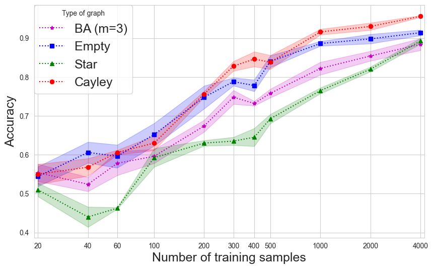
It was observed in [32] that graph neural networks tend to overfit the given graph structure, even in cases where it does no provide useful information for the predictive task. Nonetheless, it was shown that regular graphs exhibit robustness to this overfitting. As Cayley graphs are regular graphs, they exhibit this robustness.

We repeat the experiments from [32] to ensure the robustness of Cayley graphs to graph overfitting. The task is a binary classification task where the label is independent of the graph, and is computed only over the features. We used the Sum task that was presented in [32]: the label is generated using a teacher GNN that simply sums the node features and applies a linear readout to produce a scalar.

We used four different datasets from this baseline by sampling graph-structures from different graph distributions. The set of node feature vectors remains the same across all the datasets, and thus, the datasets differ only in their graph structure. The graph distributions we used are: Cayley graphs over $24$ nodes, star-graph (Star) where the only connections are between one specific node and all other nodes, and the preferential attachment model (BA)  [37], where the graph is built by incrementally adding new nodes and connecting them to existing nodes with probability proportional to the degrees of the existing nodes. We used the data as is with empty graphs (Empty) as a baseline to compare to.

On each dataset, we varied the training set size and evaluated test errors on $5$ runs with random seeds. More details on the experiment can be found in the Appendix (Section F).

The results are shown in Figure 3. The GNN trained on the Cayley graphs performs similarly to when trained on empty graphs. Nonetheless, when trained on other distributions, the performance decreases and does not recover even with $4000$ training samples. This demonstrate the robustness of Cayley graphs to graph overfitting.

Extrapolation

The ability and failures of GNNs to extrapolate to graphs of sizes larger then the one presented during training was examined in Yehudai et al. [38]. It was shown that size generalisation is dependent on local structures around each node, called d-patterns. In particular, if increasing the graph size does not change the distribution of these d-patterns, then extrapolation to larger graph sizes is guaranteed. In the context of Cayley graphs, this implies the following lemma.

Lemma 3.1.

Let $D_{G}$ be a distribution over $\mathrm{Cay}(\mathrm{SL}(k,\mathbb{Z}_{n});S_{n})$ and $D_{X}$ be a distribution over node features. Assume a node classification task with training set of infinite size sampled from $D_{G}$ and $D_{X}$. Denote the learned model by $f$. Assume that test examples are sampled from $D^{\prime}_{G}$, a distribution over $\mathrm{Cay}(\mathrm{SL}(k,\mathbb{Z}_{n^{\prime}});S_{n^{\prime}})$ where $n\neq n^{\prime}$ and $D_{X}$. Then $f$ will have zero test error.

The proof is provided in the Appendix (Section G) and it utilises the property that increasing the modulus $n$, increases the Cayley graph while preserving the regularity degree.

4 Cayley Graph Propagation

In the previous sections, we provided theoretical motivations for our proposed method of utilising the complete Cayley graph structure. The setup for CGP closely aligns with that of EGP in most aspects. We continue to consider the input to a GNN as a node feature matrix ${\bf X}\in\mathbb{R}^{|V|\times d}$ and an adjacency matrix ${\bf A}\in\mathbb{R}^{|V|\times|V|}$, which can be fed in an edge-list manner.

Additionally, the construction of the Cayley graph $\mathrm{Cay}(\mathrm{SL}(2,\mathbb{Z}_{n});S_{n})$ is still done by choosing the smallest $n$ such that $|V(\mathrm{Cay}(\mathrm{SL}(2,\mathbb{Z}_{n});S_{n}))|\geq|V|$. However, we no longer truncate the Cayley graph such that a subgraph ${\bf A}^{\text{Cay}(n)}_{1:|V|,1:|V|}$ is extracted – instead, we opt for a different approach of retaining all of the nodes of the Cayley graph, and its corresponding adjacency matrix ${\bf A}^{\text{Cay}(n)}$.

This construction requires us to add new nodes into the graph; hence, we need to modify the feature matrix into an extended version, ${\bf X}^{\text{Cay}(n)}\in\mathbb{R}^{|V(\mathrm{Cay}(n))|\times d}$. To construct this, we featurise the first $|V|$ nodes using the data from ${\bf X}$, and treat any additional nodes as virtual nodes, initialised in some pre-defined way. Specifically:

$${\bf X}^{\text{Cay}(n)}_{1:|V|}={\bf X}\qquad\qquad{\bf X}^{\text{Cay}(n)}_{|V|+1:|V(\text{Cay}(n)|}\sim\mathrm{InitVirt}$$ (3)

where $\mathrm{InitVirt}$ is any sampling procedure for initialising $d$-dimensional feature vectors; for example, we may choose to sample random features from $\mathcal{N}(0,1)$, or in our case initialise them to zeros.

Because EGP makes advantage of both the input graph (specified by ${\bf A}$) and the generated Cayley graph (specified by ${\bf A}^{\mathrm{Cay}(n)}$), we can also appropriately extend the original adjacency matrix, ${\bf A}$, to incorporate the new nodes. Since the input graph layers are intended to preserve the input graph topology as much as possible, one approach is to construct such a matrix $\widetilde{\bf A}\in\mathbb{R}^{|V(\mathrm{Cay}(n)|\times|V(\mathrm{Cay}(n)|}$ by adding self-edges to the virtual nodes only:

$$\widetilde{\bf A}_{1:|V|,1:|V|}={\bf A}\qquad\qquad\widetilde{\bf A}_{|V|+1:|V(\text{Cay}(n)|,|V|+1:|V(\text{Cay}(n)|}={\bf I}$$ (4)

$$\widetilde{\bf A}_{1:|V|,|V|+1:|V(\text{Cay}(n)|}=\widetilde{\bf A}_{|V|+1:|V(\text{Cay}(n)|,1:|V|}={\bf 0}$$ (5)

CGP now proceeds in the same manner as EGP: alternating GNN layers, such that every odd layer operates over the input graph—to preserve the topological information therein—and every even layer operates over the generated Cayley graph—to support bottleneck-free global communication. For a two-layer CGP model, this can be depicted as:

$${\bf H}=\mathrm{GNN}(\mathrm{GNN}({\bf X}^{\mathrm{Cay}(n)},\widetilde{\bf A};{\theta}_{1}),{\bf A}^{\mathrm{Cay}(n)};{\theta}_{2})$$ (6)

where $\theta_{1}$ and $\theta_{2}$ are the parameters of the first and second GNN layer, respectively. This implementation works with any choice of base GNN; here we may choose to take advantage of the graph isomorphism network ([39], GIN):

$$\vec{h}_{u}=\phi\left(\left(1+\epsilon\right)\vec{x}_{u}+\sum_{v\in\mathcal{N}_{u}}\vec{x}_{v}\right)$$ (7)

where $\vec{x}_{u}\in\mathbb{R}^{d}$ are the features of node $u$, $\epsilon$ is a learnable scalar, and $\phi$ is a MLP. Our experimentation in Section 5 shows that CGP is MPNN agnostic.

The final node embeddings ${\bf H}\in\mathbb{R}^{|V(\mathrm{Cay}(n)|\times k}$ may then be used for downstream node, graph or graph-level tasks. To avoid direct influence of virtual nodes in these predictions, we use only the embeddings corresponding to the original graph’s nodes, that is, ${\bf H}_{1:|V|}$, in downstream tasks.

The CGP model upholds the requirements of the four criteria (i-iv) set by Deac et al. [13]—arguably, in a more theoretically grounded way than EGP; Figure 1 and 2 provides empirical evidence of this. Specifically, the lower diameter of the graph used in CGP enhances its ability to eliminate over-squashing and bottlenecks, which is further supported by having a higher spectral gap. Furthermore, the CGP model may be able to make up for one of the limitations of the Cayley graph construction: the inability to find the best way to align it to a given input graph, mitigating the potential for stochastic effects in the process. The additional virtual nodes act as “bridges” between poorly connected communities in the Cayley graph, ameliorating any poorly-connected regions caused by misalignment.

5 Experimentation

In this section, we empirically validate the efficacy of using the complete Cayley graph structure on a range of graph classification tasks. In particular, we compare the CGP model against approaches that do not incur a computational complexity of having to examine the input graph’s structure: master node [5], fully adjacent layer (FA) [6] and EGP [13]. In addition to these comparisons, we further examine the scalability and performance of CGP against state-of-the-art graph rewiring techniques [40, 8, 9, 41, 11], leveraging the TUDataset [42] and LRGB [43]. Due to space limitations, we defer the results of the LRGB to Appendix (Section B), as well as analysing over-smoothing by measuring the Dirichlet energy of a graph to Appendix (Section E).

Table 1: Comparative performance evaluation of CGP against the baselines on the OGB. OOM denotes out-of-memory on a NVIDIA RTX 4090.

Model	ogbg-molhiv	ogbg-ppa
	Test ROC-AUC $\uparrow$	Test ACC $\uparrow$
GCN	$0.7566\pm 1.0421$	$0.5483\pm 0.0209$
+ Master Node	$0.7531\pm 0.0128$	$0.5824\pm 0.0219$
+ FA	$0.7628\pm 0.0191$	OOM
+ EGP	$0.7731\pm 0.8115$	$\textbf{0.6821}\pm 0.0045$
+ CGP	$\textbf{0.7794}\pm 1.2228$	$0.6782\pm 0.0066$
GIN	$0.7678\pm 1.8319$	$0.5888\pm 0.0441$
+ Master Node	$0.7608\pm 0.0134$	$0.6069\pm 0.0062$
+ FA	$0.7718\pm 0.0147$	OOM
+ EGP	$0.7537\pm 0.7627$	$0.6533\pm 0.119$
+ CGP	$\textbf{0.7899}\pm 0.9044$	$\textbf{0.6562}\pm 0.0147$

Experimental setting

We evaluate on the Open Graph Benchmark (OGB) [44] and TUDataset [42]. In our experiments, we prioritise a fair comparison with the only modification to the model being the use of the complete Cayley graph structure and the initialisation of the virtual nodes. Furthermore, we show that our proposed method is MPNN invariant by setting the underlying model to GCN [45] and GIN [39]. The chosen hyperparameters are in line with established foundations [44, 9] for each dataset respectively. Notably, the EGP paper limits its empirical analysis to only the graph classification tasks from OGB with GIN as the backbone GNN. Refer to Appendix (Section A) for more detail on our experimental setting and hyperparameters used for the OGB and TUDataset.

OGB

For real-world comparison and to extend the foundations of EGP, we first provide results on graph classification datasets from the OGB [44] against techniques that do not require dedicated preprocessing. ogbg-molhiv is among the largest molecule property prediction datasets within the scope of the MoleculeNet benchmark [46], thus providing emulation for real-world analysis. ogbg-ppa focuses on classifying species based on their taxa, using their protein-protein association networks [47]. Our model takes inspiration from the open-source implementation of OGB and hyperparameters as given by [44], including fixing the number of layers to 5, a hidden dimension of 300, a dropout of 50% and with the only modification being a batch size of 64. We report across 10 seeds and 5 seeds for ogbg-molhiv and ogbg-ppa respectively. Our results in Table 1 show that overall the CGP model outperforms the other approaches that do not require dedicated preprocessing; exemplified in the results for ogbg-molhiv. Moreover, CGP consistently outperforms the base GCN and GIN, which is not the case for the other baseline models that do not require dedicated preprocessing.

TUDataset

We extend our graph classification analysis by evaluating on REDDIT-BINARY, IMDB-BINARY, MUTAG, ENZYMES, PROTEINS and COLLAB from the TUDataset [42]. Significantly, these datasets were chosen under the claim of Karhadkar et al. [9] that the topology of the graphs in relation to the tasks require long-range interactions. The results reported in Table 2 are a continuation of our evaluation of CGP against the approaches that do not require dedicated preprocessing approaches as reported in Table 1. In contrast, the results reported in Table 3 are against the renowned graph rewiring techniques [40, 8, 9, 41, 11]. For both Table 2 and 3 we report the results averaged across 20 random seeds.

The hyperparameters used in Table 2 are similar to those prescribed by Karhadkar et al. [9], however, to further pinpoint with certainty that the performance gain can be credited to the utilisation of the complete Cayley graph structure we opt for those more akin to to our OGB experimentation. We set the number of layers to 5, the hidden dimension to 128 and use a dropout of 10%. The results in Table 2 underscore the effectiveness of our proposed model. For both GCN and GIN, CGP is consistently first or second across all datasets (except for one case), achieving the highest classification accuracy. This is particularly notable when the sparsity of the Cayley graphs is considered in relation to certain datasets, such as IMDB-BINARY and COLLAB. The sparse nature of the Cayley graph means that unlike many graph rewiring techniques edges may be removed; refer to Table 5 in Appendix (Section A) for the dataset statistics.

Table 2: Results of CGP compared against the baselines that do not require dedicated preprocessing for GCN and GIN on the TUDataset. OOM signifies out-of-memory on a NVIDIA RTX 4090. The colours highlight First, Second and Third.

Model	REDDIT-BINARY	IMDB-BINARY	MUTAG	ENZYMES	PROTEINS	COLLAB
GCN	${\color[rgb]{1,0,0}90.000}\pm 2.121$	$63.200\pm 5.036$	$77.500\pm 10.186$	${\color[rgb]{1,.5,0}39.083}\pm 6.465$	$71.696\pm 5.432$	$71.370\pm 2.394$
+ Master Node	${\color[rgb]{0,0,1}85.425}\pm 2.830$	${\color[rgb]{0,0,1}64.600}\pm 5.342$	${\color[rgb]{0,0,1}86.000}\pm 7.842$	$36.583\pm 5.904$	$72.277\pm 3.927$	${\color[rgb]{1,0,0}73.590}\pm 1.694$
+ FA	OOM	$62.500\pm 5.296$	${\color[rgb]{1,.5,0}84.500}\pm 7.890$	${\color[rgb]{0,0,1}41.917}\pm 7.116$	${\color[rgb]{0,0,1}73.259}\pm 4.397$	${\color[rgb]{1,.5,0}71.980}\pm 2.413$
+ EGP	${\color[rgb]{1,.5,0}82.075}\pm 3.568$	${\color[rgb]{1,.5,0}64.400}\pm 3.980$	$80.250\pm 7.980$	$38.917\pm 7.017$	${\color[rgb]{1,.5,0}72.634}\pm 2.545$	$70.090\pm 2.225$
+ CGP	$81.900\pm 2.691$	${\color[rgb]{1,0,0}65.300}\pm 4.540$	${\color[rgb]{1,0,0}89.250}\pm 8.983$	${\color[rgb]{1,0,0}49.000}\pm 6.200$	${\color[rgb]{1,0,0}74.330}\pm 3.992$	${\color[rgb]{0,0,1}72.430}\pm 1.930$
GIN	$89.500\pm 3.066$	${\color[rgb]{1,.5,0}71.800}\pm 0.817$	$87.250\pm 9.284$	$44.583\pm 7.320$	$69.911\pm 4.792$	$71.410\pm 2.470$
+ Master Node	${\color[rgb]{1,0,0}91.600}\pm 1.868$	$70.400\pm 3.611$	${\color[rgb]{1,.5,0}87.250}\pm 7.822$	$46.083\pm 6.396$	${\color[rgb]{1,.5,0}73.170}\pm 3.793$	${\color[rgb]{1,.5,0}72.920}\pm 2.394$
+ FA	OOM	${\color[rgb]{1,0,0}73.150}\pm 3.554$	$85.500\pm 10.235$	${\color[rgb]{1,0,0}55.083}\pm 5.974$	${\color[rgb]{0,0,1}73.304}\pm 3.000$	${\color[rgb]{0,0,1}73.310}\pm 1.720$
+ EGP	${\color[rgb]{1,.5,0}90.125}\pm 1.870$	$69.850\pm 4.028$	${\color[rgb]{0,0,1}88.500}\pm 7.599$	${\color[rgb]{1,.5,0}51.333}\pm 6.227$	$72.545\pm 4.319$	$72.820\pm 2.819$
+ CGP	${\color[rgb]{0,0,1}90.175}\pm 1.705$	${\color[rgb]{0,0,1}72.200}\pm 2.804$	${\color[rgb]{1,0,0}91.000}\pm 9.301$	${\color[rgb]{0,0,1}52.667}\pm 6.442$	${\color[rgb]{1,0,0}73.438}\pm 3.013$	${\color[rgb]{1,0,0}74.420}\pm 2.202$

Table 3: Results of CGP compared against EGP and the graph rewiring techniques for GCN and GIN on the TUDataset. The experimental setup uses the setting as in Karhadkar et al. [9], and hyperparameters for each graph rewiring approach from [40, 8, 9, 41, 11]. The colours highlight First, Second and Third. OOT indicates out-of-time for the prepreprocessing rewiring time.

Model	REDDIT-BINARY	IMDB-BINARY	MUTAG	ENZYMES	PROTEINS	COLLAB
GCN	$77.735\pm 1.586$	${\color[rgb]{0,0,1}60.500}\pm 2.729$	$74.750\pm 4.030$	${\color[rgb]{1,.5,0}29.083}\pm 2.363$	$66.652\pm 1.933$	${\color[rgb]{1,.5,0}70.490}\pm 1.628$
+ DIGL	$77.350\pm 1.206$	$49.600\pm 2.435$	$70.500\pm 5.045$	${\color[rgb]{0,0,1}30.833}\pm 1.537$	$72.723\pm 1.420$	$56.470\pm 0.865$
+ SDRF	${\color[rgb]{0,0,1}77.975}\pm 1.479$	$59.000\pm 2.254$	$74.000\pm 3.462$	$26.667\pm 2.000$	$67.277\pm 2.170$	${\color[rgb]{0,0,1}71.330}\pm 0.807$
+ FoSR	${\color[rgb]{1,.5,0}77.750}\pm 1.385$	${\color[rgb]{1,.5,0}59.750}\pm 2.357$	$75.250\pm 5.722$	$24.167\pm 3.005$	$70.848\pm 1.618$	$67.220\pm 1.367$
+ BORF	OOT	$48.900\pm 0.900$	${\color[rgb]{0,0,1}76.750}\pm 0.037$	$27.833\pm 0.029$	$67.411\pm 0.016$	OOT
+ GTR	${\color[rgb]{1,0,0}79.025}\pm 1.248$	${\color[rgb]{1,0,0}60.700}\pm 2.079$	${\color[rgb]{1,.5,0}76.500}\pm 4.189$	$25.333\pm 2.931$	${\color[rgb]{1,.5,0}72.991}\pm 1.956$	${\color[rgb]{1,0,0}72.600}\pm 1.025$
+ EGP	$67.550\pm 1.200$	$59.700\pm 2.371$	$70.500\pm 4.738$	$27.583\pm 3.262$	${\color[rgb]{1,0,0}73.304}\pm 2.516$	$69.470\pm 0.970$
+ CGP	$67.050\pm 1.483$	$56.200\pm 1.825$	${\color[rgb]{1,0,0}83.750}\pm 3.597$	${\color[rgb]{1,0,0}31.000}\pm 2.397$	${\color[rgb]{0,0,1}73.036}\pm 1.291$	$69.630\pm 0.730$
GIN	${\color[rgb]{1,.5,0}84.600}\pm 1.454$	${\color[rgb]{0,0,1}71.250}\pm 1.509$	$80.500\pm 5.143$	$35.667\pm 2.803$	$70.312\pm 1.749$	$71.490\pm 0.746$
+ DIGL	$84.575\pm 1.265$	$52.650\pm 2.150$	$78.500\pm 4.189$	${\color[rgb]{0,0,1}41.500}\pm 3.063$	${\color[rgb]{0,0,1}72.321}\pm 1.440$	$57.620\pm 1.010$
+ SDRF	$84.550\pm 1.396$	$69.550\pm 2.381$	${\color[rgb]{1,.5,0}80.500}\pm 4.177$	$37.167\pm 2.709$	$69.509\pm 1.709$	${\color[rgb]{0,0,1}72.958}\pm 0.419$
+ FoSR	${\color[rgb]{1,0,0}85.750}\pm 1.099$	$69.250\pm 1.810$	$80.500\pm 4.738$	$28.083\pm 2.301$	$71.518\pm 1.767$	$71.720\pm 0.892$
+ BORF	OOT	${\color[rgb]{1,.5,0}70.700}\pm 0.018$	$79.250\pm 0.038$	$34.167\pm 0.029$	$70.625\pm 0.017$	OOT
+ GTR	${\color[rgb]{0,0,1}85.474}\pm 0.826$	$69.550\pm 1.473$	$79.000\pm 3.847$	$31.750\pm 2.466$	${\color[rgb]{1,.5,0}72.054}\pm 1.510$	$71.849\pm 0.710$
+ EGP	$77.875\pm 1.563$	$68.250\pm 1.121$	${\color[rgb]{0,0,1}81.500}\pm 4.696$	${\color[rgb]{1,.5,0}40.667}\pm 3.095$	$70.848\pm 1.568$	${\color[rgb]{1,.5,0}72.330}\pm 0.954$
+ CGP	$78.225\pm 1.268$	${\color[rgb]{1,0,0}71.650}\pm 1.532$	${\color[rgb]{1,0,0}85.250}\pm 3.200$	${\color[rgb]{1,0,0}50.083}\pm 2.242$	${\color[rgb]{1,0,0}73.080}\pm 1.396$	${\color[rgb]{1,0,0}73.350}\pm 0.788$

In Table 3 we compare CGP against the baselines, including the state-of-the-art graph rewiring techniques: DIGL [40], SDRF [8], FoSR [9], BORF [41] and GTR [11]. However, in this instance we use the experimental setting and hyperparameters set by Karhadkar et al. [9], which are commonly used across the aforementioned graph rewiring techniques. By applying these hyperparameters, we not only ensure a fair comparison, but showcase that CGP continues to be competitive even under their conditions. The hyperparameters include a hidden dimension of 64, the number of layers set to 4 and a dropout of 50%. Finally, Karhadkar et al. [9] reports the results with a 95% confidence interval. Thus, we respect this for decision Table 3. Notably, we report OOT to indicate out-of-time for the preprocessing rewiring procedure for BORF on the REDDIT-BINARY and COLLAB datasets. This is in accordance with Nguyen et al. [41] who do not report results for these two datasets and corresponding hyperparameters. In addition, a time-out is reported in [48] for the aforementioned datasets, whilst in [49] they report out-of-memory for COLLAB. In Appendix (Section C) we conduct a scalability analysis in which we provide the graph rewiring time for each of our baseline models, as well as extending this beyond the real-world datasets through a synthetic benchmark.

The results in Table 3 underscore the effectiveness of CGP in comparison with the graph rewiring techniques. In particular, in the case of GIN, our CGP model obtains the highest accuracy for all datasets except for REDDIT-BINARY. The overall performance of CGP when applied to GCN is not as competitive as those of GIN, however our results are still comparable with the other graph rewiring techniques. CGP obtains the highest accuracy in two of the datasets, only placing second to GTR. Collectively, our results are consistent with our previously discussed limitations regarding the sparsity of CGP when applied to datasets with a significantly higher edge-to-node ratio. However, the results of CGP for GIN recover this loss in performance for IMDB-BINARY and COLLAB, emphasising the work of You et al. [50] in which the design space of GNNs can greatly impact a model’s results. This is supplemented by the results reported in Table 2 in which IMDB-BINARY for GCN obtains the highest classification accuracy. Finally, of significance is the parity of the hyperparameter’s number of layers; Table 2 uses 5 layers, whereas Table 3 uses 4 layers. This demonstrates the performance of CGP is irrespective of the final layer being the input or Cayley graph.

Ablation studies

In the following, we answer the question: ‘is the complete Cayley graph structure a suitable alternative to a fully adjacent layer [6]?’. In Table 4 we show that it is a promising avenue as the results for CGP^† and FA^† are similar for both GCN and GIN. However, the sparsity of CGP is highlighted in the results of REDDIT-BINARY, whereby FA runs out-of-memory (OOM). Accordingly, these results demonstrate the advantages of CGP, due to it being far more scalable. Notably, the results reported in Table 4 use the same experimental setting and hyperparameters as Table 2.

Next, we investigate in accordance with the recent work of Bechler-Speicher et al. [51]; we examine if we can ignore the input graph entirely and solely propagate over the Cayley graph structure. Our results in Table 4 conclude that the inductive bias endowed from the input graph is required. The baseline procedure of CGP (interweaving a Cayley graph with an input graph), and using a Cayley graph for the last layer only, outperforms using a Cayley graph solely for each layer. One explanation is that the interweaving schema of CGP aligns with the principles of JK networks [52], facilitating improved structure-aware representations by varying the neighbourhood ranges. However, the tone set by Bechler-Speicher et al. [51] is still a promising line of research, as the results of PROTEINS indicates that the optimal graph-structure used is still task dependent.

Table 4: Results of CGP using the Cayley graph in different layer approaches compared against FA on the TUDataset. $\dagger$ denotes last layer and $\ast$ denotes every layer. OOM is out-of-memory on a NVIDIA RTX 4090. The colours highlight First, Second and Third.

Model	REDDIT-BINARY	IMDB-BINARY	MUTAG	ENZYMES	PROTEINS	COLLAB
GCN	${\color[rgb]{1,0,0}90.000}\pm 2.121$	${\color[rgb]{0,0,1}63.200}\pm 5.036$	$77.500\pm 10.186$	$39.083\pm 6.465$	$71.696\pm 5.432$	${\color[rgb]{1,.5,0}71.370}\pm 2.394$
+ FA†	OOM	${\color[rgb]{1,.5,0}62.500}\pm 5.296$	${\color[rgb]{1,.5,0}84.500}\pm 7.890$	${\color[rgb]{1,.5,0}41.917}\pm 7.116$	${\color[rgb]{1,.5,0}73.259}\pm 4.397$	${\color[rgb]{0,0,1}71.980}\pm 2.413$
+ FA∗	OOM	$48.800\pm 6.547$	$81.500\pm 9.631$	$29.667\pm 4.989$	$71.786\pm 2.452$	$42.940\pm 14.368$
+ CGP	${\color[rgb]{1,.5,0}81.900}\pm 2.691$	${\color[rgb]{1,0,0}65.300}\pm 4.540$	${\color[rgb]{1,0,0}89.250}\pm 8.983$	${\color[rgb]{1,0,0}49.000}\pm 6.200$	${\color[rgb]{1,0,0}74.330}\pm 3.992$	${\color[rgb]{1,0,0}72.430}\pm 1.930$
+ CGP†	${\color[rgb]{0,0,1}89.600}\pm 1.736$	$61.850\pm 5.850$	$78.750\pm 9.601$	${\color[rgb]{0,0,1}42.000}\pm 4.522$	$71.250\pm 3.989$	$71.360\pm 1.663$
+ CGP∗	$70.250\pm 3.673$	$54.550\pm 4.295$	${\color[rgb]{0,0,1}88.500}\pm 7.921$	$35.750\pm 5.664$	${\color[rgb]{0,0,1}73.259}\pm 3.346$	$56.170\pm 2.412$
GIN	${\color[rgb]{1,.5,0}89.500}\pm 3.066$	$71.800\pm 0.817$	${\color[rgb]{1,.5,0}87.250}\pm 9.284$	$44.583\pm 7.320$	$69.911\pm 4.792$	$71.410\pm 2.470$
+ FA†	OOM	${\color[rgb]{1,0,0}73.150}\pm 3.554$	$85.500\pm 10.235$	${\color[rgb]{1,0,0}55.083}\pm 5.974$	${\color[rgb]{1,.5,0}73.304}\pm 3.000$	${\color[rgb]{1,.5,0}73.310}\pm 1.720$
+ FA∗	OOM	$54.250\pm 4.784$	$83.750\pm 7.224$	$34.250\pm 4.669$	$71.250\pm 4.721$	$55.270\pm 1.604$
+ CGP	${\color[rgb]{0,0,1}90.175}\pm 1.705$	${\color[rgb]{1,.5,0}72.200}\pm 2.804$	${\color[rgb]{1,0,0}91.000}\pm 9.301$	${\color[rgb]{0,0,1}52.667}\pm 6.442$	${\color[rgb]{0,0,1}73.438}\pm 3.013$	${\color[rgb]{1,0,0}74.420}\pm 2.202$
+ CGP†	${\color[rgb]{1,0,0}90.200}\pm 1.749$	${\color[rgb]{0,0,1}72.900}\pm 4.381$	${\color[rgb]{0,0,1}90.000}\pm 5.701$	${\color[rgb]{1,.5,0}51.417}\pm 6.714$	$71.741\pm 4.667$	${\color[rgb]{0,0,1}73.760}\pm 1.664$
+ CGP∗	$75.775\pm 3.378$	$53.250\pm 4.276$	$85.500\pm 7.730$	$37.167\pm 6.261$	${\color[rgb]{1,0,0}74.330}\pm 4.177$	$57.820\pm 2.172$

6 Conclusion

In this work, we presented Cayley Graph Propagation (CGP), an efficient propagation scheme that mitigates over-squashing. CGP utilises the complete Cayley Graph structure to guarantee improved information flow between nodes in the input graph. We highlight the advantages of Cayley graphs as expanders and regular graphs. We show that by truncating the Cayley graphs to align with the input graph, as suggested in Expander Graph Propagation, the resulting graph may contain bottlenecks. This is in contrast to the Cayley graph we use, which is guaranteed to be bottleneck-free. We demonstrate the effectiveness and efficiency of CGP compared to EGP and other rewiring approaches, over multiple real-world datasets, including large-scale and long-range datasets.

Limitations and Future Work

One limitation of our proposed model is the performance on datasets containing graphs with a comparatively higher node-to-edge ratio. For this reason, one such avenue for future work is aligning the Cayley graph edges such that that they retain the inductive bias of the task [33]. Additionally, it would be interesting to see how CGP performs in other tasks that utilise expander graphs, including but not limited to temporal graph rewiring [31]. Furthermore, concurrent work has used virtual nodes as the focal point of their proposed methods [53, 54] with Southern et al. [55] analysing virtual nodes’ role within the context of over-squashing. Therefore, we theorise an interesting setting would be applying these authors’ approaches to the additional virtual nodes retained from the complete Cayley graph structure.

Appendix A Experimental Details

Table 5: Statistics of the datasets from OGB, TUDataset and LRGB used as part of our evaluation.

Dataset	#Graphs	Average #Nodes	Average #Edges	#Classes
OGBG-MOLHIV	41,127	25.5	27.5	2
OGBG-PPA	158,100	243.4	2,266.1	37
REDDIT-BINARY	2,000	429.6	995.5	2
IMDB-BINARY	1,000	19.8	193.1	2
MUTAG	188	17.9	39.6	2
ENZYMES	600	32.6	124.3	6
PROTEINS	1,113	39.1	145.6	2
COLLAB	5,000	74.5	4,914.4	3
PEPTIDES-FUNC	15,535	150.94	307.30	10
PEPTIDES-STRUCT	15,535	150.94	307.30	11

In this section, we provide thorough details regarding our experimental setting for each of our datasets. We utilise the well-established experimental settings [44, 9] that are used for OGB and TUDataset respectively. The experimental setting for the LRGB [43] is found in Section B. Refer to Table 5 for the dataset statistics. Of significance, to rule out performance gain due to hyperparameter tuning in our results we use the same setting of GNN and hyperparameters for each task and model. All of our experiments use the default settings of the Adam optimiser [56] with a learning rate of $1\times 10^{-3}$, however the TUDataset and LRGB use the ReduceLROnPlateau scheduler with differing parameters.

A.1 Datasets

OGB Datasets

From the OGB [44] we consider two of the graph classification tasks: ogbg-molhiv and ogbg-ppa. ogbg-molhiv is among the largest molecule property prediction datasets within the scope of the MoleculeNet benchmark [46], and ogbg-ppa focuses on classifying species based on their taxa, using their protein-protein association networks [47]. The OGB provides a unified evaluation protocol for each dataset, including application-specific data splits and evaluation metrics. Accordingly, our experimental setup to empirically evaluate against the OGB datasets leverages the official open-source implementation from the OGB authors [44]. ogbg-molhiv uses a 80%/10%/10% train/validation/test split and ROC-AUC for the evaluation metric, whilst ogbg-ppa uses a 50%/28%/22% train/validation/test split and accuracy for the evaluation metric. The hyperparameter setting for our models includes 5 layers, a hidden dimension of 300, a dropout of 50% and the use of Batch Norm [57]. In Table 1 the results reported for our model are trained to 100 epochs across 10 seeds and 5 seeds for ogbg-molhiv and ogbg-ppa respectively.

TUDataset

The TUDataset [42] is considered under the claim of Karhadkar et al. [9] that the topology of the graphs in relation to the tasks require long-range interactions. Thus, we consider all graph classification tasks from the TUDataset: REDDIT-BINARY, IMDB-BINARY, MUTAG, ENZYMES, PROTEINS and COLLAB. Our experimental setup for the TUDataset is akin to the well-established and open-source setting of Karhadkar et al. [9]. Accordingly, we train our GNNs with 80%/10%/10% train/validation/test split and use a stopping patience of 100 epochs based on the validation loss. The ReduceLROnPlateu uses the default setting as found in PyTorch [58]. However unlike Karhadkar et al. [9], we report the accuracy over 20 random seeds and set the maximum number of epochs to 300 [48]. Additionally, in line with our OGB setup we apply Batch Norm [57]. The results reported in Table 2 use a model that is more akin to our OGB experimental setup, therefore our hyperparameters include setting the number of layers to 5, a hidden dimension of 128 and a dropout of 10%.

For Table 3, we use the hyperparameters as in the well-established graph rewiring baselines: DIGL [40], SDRF [8], FoSR [9], BORF [41] and GTR [11]. By adopting the hyperparameters of these baselines methods, we not only ensure a fair comparison, but demonstrate that CGP remains competitive even under their prescribed conditions. To this end, in Table 3 and as in Karhadkar et al. [9] we use 4 layers, a hidden dimension of 64 and a dropout of 50%. Additionally, in accordance with Karhadkar et al. [9] the results in Table 3 are reported to a 95% confidence interval. We report the standard deviation $\sigma$ for all other tables, due to this being more commonly used within the community. For the graph rewiring techniques, we follow the hyperparameters as reported in the respective baselines. This includes the teleport probability ($\alpha$) and sparsification threshold ($\epsilon$) for DIGL, as well as the number of rewiring iterations for SDRF and FoSR being derived from Karhadkar et al. [9]. For BORF this includes the number of batches ($n$), number of edges added per batch ($h$), and number of edges removed per batch ($k$) from Nguyen et al. [41]. Finally, for GTR this includes the number of edges added from Black et al. [11].

A.2 Hardware

All of our experimentation was conducted on a local machine with an AMD Ryzen 9 7950X3D 16-Core Processor (4.20 GHz), NVIDIA RTX 4090 ($24$ GB) and $64$ GB of RAM. The only exception is the OGBG-PPA results in which some of the baselines were processed on an external server with $8\times$ NVIDIA QUADRO RTX 8000 ($48$ GB). The following libraries were used as part of the implementation PyTorch [58], PyTorch Geometric [59] and NumPy [60].

Appendix B Additional Experiments

In this section, we provide additional results to solidify the efficacy of our CGP model by comparing it against state-of-the-art graph rewiring techniques [8, 9] and EGP [13] on the Long Range Graph Benchmark (LRGB) [43].

Table 6: Comparative performance evaluation of CGP against graph rewiring techniques on the LRGB.

Model	Peptides-func	Peptides-struct
	Test AP $\uparrow$	Test MAE $\downarrow$
GCN	$0.5029\pm 0.0058$	$0.3587\pm 0.0006$
+ SDRF	$0.5041\pm 0.0026$	$0.3559\pm 0.0010$
+ FoSR	$0.4534\pm 0.0090$	$0.3003\pm 0.0007$
+ EGP	$0.4972\pm 0.0023$	$0.3001\pm 0.0013$
+ CGP	$\textbf{0.5106}\pm 0.0014$	$\textbf{0.2931}\pm 0.0006$
GIN	$0.5124\pm 0.0055$	$0.3544\pm 0.0014$
+ SDRF	$0.5122\pm 0.0061$	$0.3515\pm 0.0011$
+ FoSR	$0.4584\pm 0.0079$	$0.3008\pm 0.0014$
+ EGP	$0.4926\pm 0.0070$	$0.3034\pm 0.0027$
+ CGP	$\textbf{0.5159}\pm 0.0059$	$\textbf{0.2910}\pm 0.0011$

Datasets

We consider the Peptides datasets from the Long Range Graph Benchmark (LRGB) [43], which have two related tasks Peptides-func and Peptides-struct. The former is a peptide feature classification task in which the objective is to predict the peptide function out of 10 classes with the performance being measured by Average Precision (AP). The latter consists of the same graphs as Peptides-func, however instead it is a graph regression task in which the aim is to predict aggregated 3D properties of the peptides at the graph level; the performance metric is Mean Absolute Error (MAE). The dataset statistics for the LRGB can be found in Table 5.

Experimental details

Similar to the OGB, the LRGB [43] provides an experimental setting with the aim to have unified experimental evaluation of their benchmarks. Correspondingly, we leverage the LRGB implementation that is built upon the GraphGym module [50]. For both Peptides tasks it uses a 70%/15%/15% train/validation/test split. The experimental setup of Dwivedi et al. [43] fixes the models number of layers to 5, and does not use dropout, but it does use Batch Norm [57]. However, we reduce the models number of parameters using a hidden dimension of 64 as in Nguyen et al. [41], as opposed to 300 [43]. Additionally, we reduce the number of epochs to 250, which is in line with Tönshoff et al. [61]. A ReduceLROnPlateau scheduler is used following Dwivedi et al. [43] settings of a patience of 20 epochs, a decay factor of 0.5 and a minimum learning rate of $1\times 10^{-5}$. We use the graph rewiring hyperparameters from [41, 49].

Results

The results in Table 6 showcase that CGP outperforms the state-of-the-art graph rewiring approaches, as well as EGP for both GCN and GIN. However, it is noted that the work of Tönshoff et al. [61] achieves improved performance through extensive hyperparameter tuning. Nevertheless, this is beyond the scope of evaluating the impact of using the complete Cayley graph structure.

Appendix C Scalability Analysis of CGP

Figure 4: Synthetic preprocessing benchmark for CGP in regards to graph rewiring techniques, using Erdős–Rényi graphs with a probability $p=\frac{5\log n}{n}$. Left: Preprocessing time of CGP against DIGL, FoSR and GTR. Right: Preprocessing time of CGP against SDRF.

Table 7: Preprocess graph rewiring runtime (in seconds) for each graph in the TUDataset. OOT indicates out-of-time for the prepreprocessing rewiring time.

Model	REDDIT-BINARY	IMDB-BINARY	MUTAG	ENZYMES	PROTEINS	COLLAB
DIGL	40.3837	0.411771	0.0342833	0.243485	0.491458	56.3175
SDRF	359.128	5.13257	0.669701	1.71482	3.02873	619.125
FoSR	74.8568	4.54634	4.71567	4.56855	5.04358	9.79994
BORF	OOT	465.408	53.7069	179.573	351.173	OOT
GTR	118.549	3.39839	1.54127	2.87399	6.49714	92.6125
EGP	0.245215	0.0185697	0.00446963	0.0163198	0.0393348	0.129567
CGP	0.226065	0.0211341	0.00438905	0.0166841	0.0348585	0.131188

Table 8: Preprocess runtime (in seconds) for state-of-the-art graph rewiring techniques for each graph in the LRGB dataset.

Model	Peptides-func	Peptides-struct
SDRF	61.0356	56.1561
FoSR	23.4263	24.1858
EGP	1.36170	1.29376
CGP	1.27776	1.29608

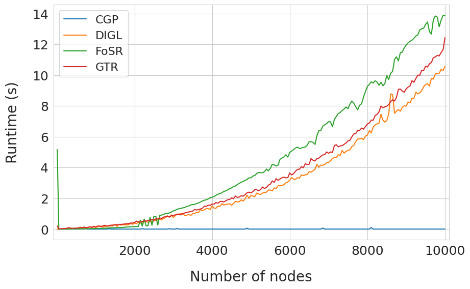
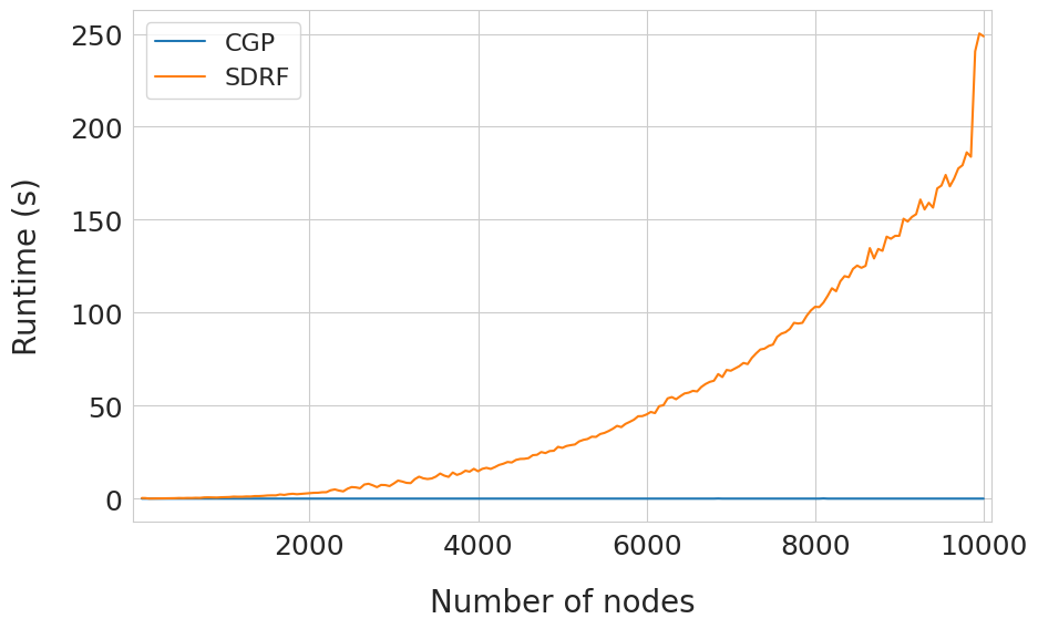
We empirically analyse the scalability of CGP by comparing the computational preprocessing time against the state-of-the-art graph rewiring techniques [40, 8, 9, 41, 11]. We first provide a real-world evaluation by benchmarking the preprocessing time on two real-world datasets: TUDataset [42] and LRGB [43]. The results are reported in Table 7 and 8, using the same graph rewiring techniques as in Table 3 and 6 respectively. To extend our scalability analysis, we create a synthetic benchmark by leveraging Erdős–Rényi with a probability $p=\frac{5\log n}{n}$ (as used by Karhadkar et al. [9]) to create graphs of up to 10,000 nodes. In line with the results reported in Table 3, we do not conduct the synthetic benchmark for BORF [41], due to the impracticality of the rewiring time which is highlighted in Section 5.

The results show the efficacy of our proposed CGP model, as the preprocessing time is orders of magnitude lower than the graph rewiring techniques. To this end, we examine the lack of computational preprocessing time required to generate the corresponding Cayley graphs for both CGP and EGP. Overall, our results show the practicality of CGP to scale to large graphs when compared to the graph rewiring approaches. This is reinforced by the experimentation being conducted on the local machine with leading hardware as in Section A.2. In particular, both the CPU and GPU deliver top-tier clock speeds, therefore on lower-performing hardware, the graph rewiring techniques could have a more detrimental effect.

Appendix D Effective Resistance of Cayley graphs

(a) MUTAG

(b) ENZYMES

(c) PROTEINS

(d) IMDB-BINARY

(e) COLLAB

(f) OGBG-MOLHIV

Figure 5: Comparison of the total effective resistance $R_{tot}$ for CGP against the baseline model and EGP. A lower total effective resistance indicates that a graph is less susceptible to over-squashing.

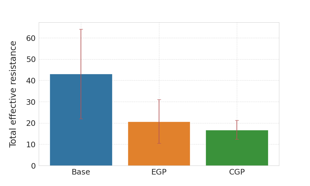
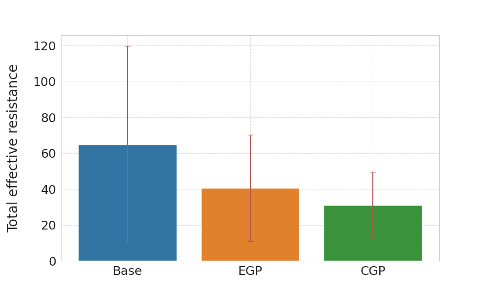
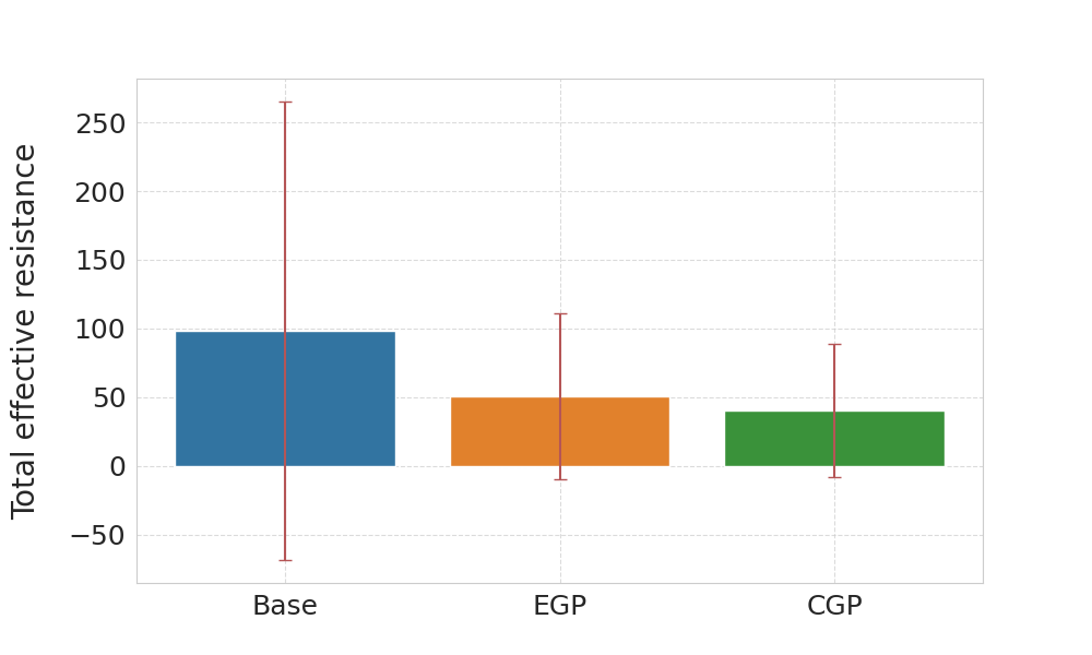
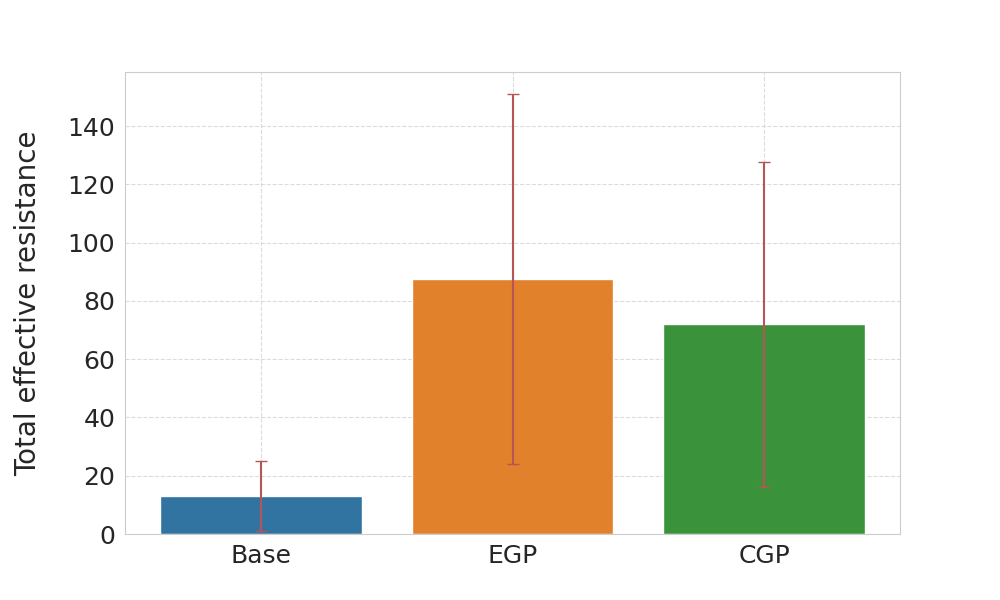
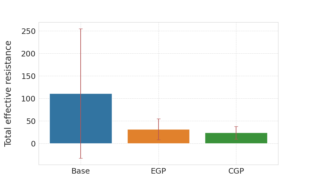
In this work, we have used the Cheeger constant as an approach to measure bottlenecks in a graph [62] in regards to over-squashing. An alternative closely related approach is measuring over-squashing through the lens of effective resistance [11]. Stemming from the field of electrical engineering, the effective resistance between two nodes $u$ and $v$ reflects the ease of current flow. In turn, this concept has become analogous to measuring the connectivity between nodes within graph theory. Formally, the effective resistance between two nodes $u$ and $v$ can be expressed using the pseudoinverse ${\bf L}^{+}$ of $\mathbf{L}$, $R_{u,v}=({\bf 1}_{u}-{\bf 1}_{v})^{\mathsf{T}}{\bf L}^{+}({\bf 1}_{u}-{\bf 1}_{v})$, where ${\bf 1}_{u}$ and ${\bf 1}_{v}$ are indicators for nodes $u$ and $v$.

The total effective resistance $R_{tot}$ then builds upon this by measuring the effective resistance for all pairs of nodes within a graph, thus providing a metric to quantify over-squashing in a graph. As per Black et al. [11], the total effective resistance $R_{tot}$ is given by:

$$R_{tot}\,=\,\sum_{u>v}R_{u,v}\,=\,n\cdot\mathrm{Tr}(\mathbf{L}^{+})\,=\,n\sum_{i=1}^{n-1}\frac{1}{\lambda_{i}}.$$ (8)

The results in Figure 5 show the average of the total effective resistance $R_{tot}$ for all the corresponding Cayley graphs against the base input graphs and truncated Cayley graphs as found in EGP. Akin to the results presented in Black et al. [11], for a fair evaluation we do not include graphs that may be disconnected. This is because the Cayley graphs used in CGP are a complete and regular graph structure, therefore every node will be connected. The results show that CGP consistently has a lower total effective resistance $R_{tot}$ in comparison to EGP. Significantly, the complete Cayley graph structure is chosen by recalling $|V(\mathrm{Cay}(\mathrm{SL}(2,\mathbb{Z}_{n});S_{n}))|\geq|V|$, therefore the total effective resistance $R_{tot}$ for CGP may be inflated due to it potentially being summed over more pairs of nodes. This further reinforces our claim that it is more beneficial to use the complete Cayley graph structure with the additional nodes serving as shortcuts for message passing between nodes along the graph.

In line with our results reported in our empirical evaluation, for certain datasets the total effective resistance for EGP and CGP is higher than the base input graph. The statistics of the datasets reported in Table 5 provide evidence to explain this observation; IMDB-BINARY and COLLAB have a significantly higher edge-to-node ratio when compared to the more sparse Cayley graph’s structure. Nevertheless, our results reported in Table 2 illustrate that the CGP model counteracts this by still providing leading performance on these datasets.

Appendix E Dirichlet Energy of Cayley graphs

(a) MUTAG

(b) ENZYMES

(c) PROTEINS

Figure 6: Comparison of the Dirichlet energy for CGP against the baseline model, FA and EGP for the TUDataset. A higher energy indicates that the proposed approach is more robust to the over-smoothing problem.

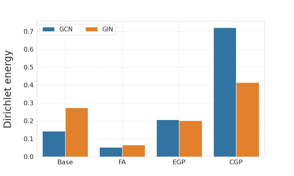
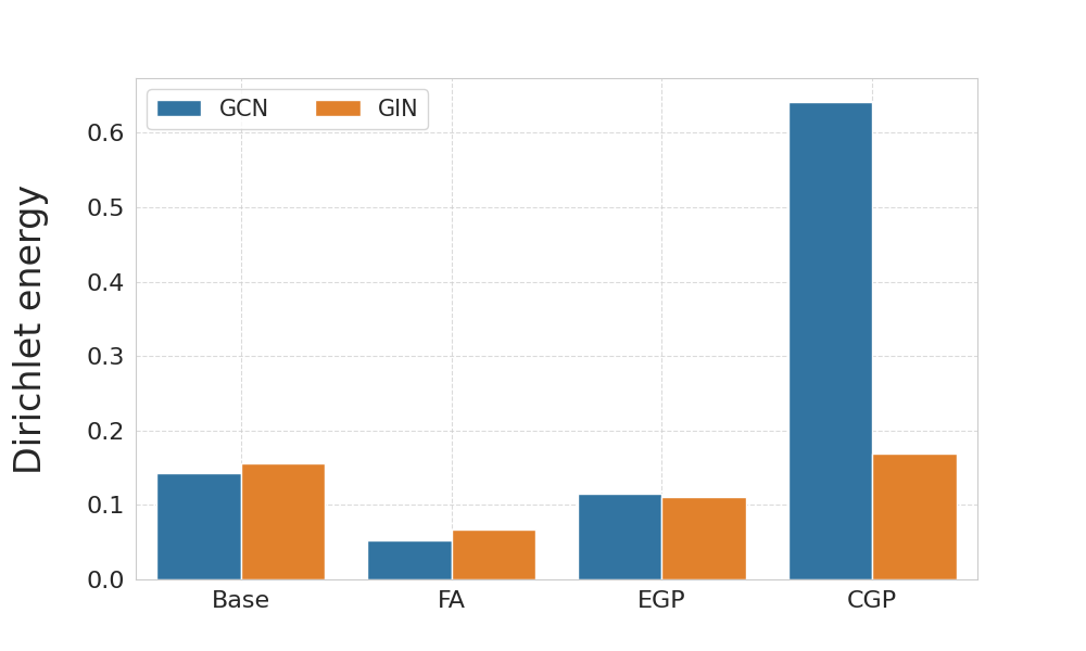
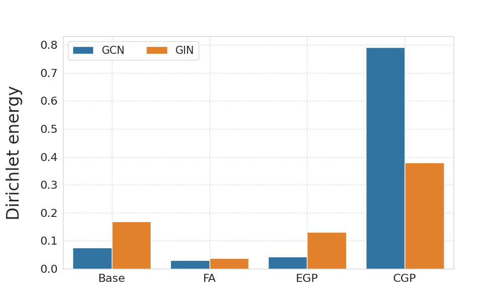
Here, we evaluate the impact of propagating over the complete Cayley graph structure in regards to the over-smoothing problem using the Dirichlet energy. As stated in Section 1, a trade-off occurs between mitigating over-squashing and causing over-smoothing. The Dirichlet energy quantifies over-smoothing by measuring the deviation of a function on the graph from being constant between connected node pairs, thus indicating the level of non-smoothness in the signals [34]. In turn, the Dirichlet energy has been used to measure the amount of over-smoothing in graph representations [9, 12, 48].

Similar to EGP [13] and FA [6], the CGP model uses an independent graph structure to propagate information over, as opposed to the graph rewiring approaches in which they directly alter the input graph structure. Consequently, we conduct our Dirichlet energy analysis against EGP and FA, which also fall under the category of approaches that do not require dedicated preprocessing. The results in Figure 6 show that CGP consistently obtains a higher Dirichlet energy for both GCN and GIN when compared to EGP and FA. This further highlights the strengths of the CGP model to mitigate over-squashing, whilst minimising the negative implications of over-smoothing through the use of the additional virtual nodes retained from the complete Cayley graph structure.

Appendix F Additional Experiment Details for Section 3.2

Sum Task

This is a binary classification synthetic task with a graph-less ground truth function. To generate the label, we use a teacher GNN that simply sums the node features and applies a linear readout to produce a scalar. The data contains non-informative graph-structures which are drawn from the GNP graph distribution [63], where the edges are sampled i.i.d with probability $p$ (we used $p=0.5$).

The teacher readout is sampled once from $\mathcal{N}(0,1)$ and used for all the graphs. All graphs have $n=20$ nodes, and each node is assigned with a feature vector in $\mathbb{R}^{128}$ sampled i.i.d from $\mathcal{N}(0,1)$.

We used a $1$-layer “student" GNN following the teacher model, with readout and ReLU activations.

We evaluated the learning curve with an increasing amount of $\{20,40,60,100,200,300,400,500,1000,2000,4000\}$ samples. We note that the GNN has a total of $\sim$16,000 parameters, and thus, it is over-parameterised and can fit the training data with perfect accuracy.

Appendix G Proof of Lemma 3.1

We consider the case of a node classification task over Cayley graphs. We wish to show that if the training data consists of infinitely many samples from a distribution over $\mathrm{Cay}(\mathrm{SL}(k,\mathbb{Z}_{n});S_{n})$, then the learned model will extrapolate perfectly to a distribution over graphs drawn from $\mathrm{Cay}(\mathrm{SL}(k,\mathbb{Z}_{n^{\prime}});S_{n^{\prime}})$, where $n\neq n$. We assume the same feature distribution in all cases.

Let $f$ be a node classifier with perfect accuracy on the support of the training distribution.

Let $G=(X_{G},A_{\mathrm{Cay}(\mathrm{SL}(k,\mathbb{Z}_{n});S_{n})})$ be in the support of the training distribution and $v$ a vertex in $G$. Let $G^{\prime}=(X_{G},A_{\mathrm{Cay}(\mathrm{SL}(k,\mathbb{Z}_{n^{\prime}});S_{n^{\prime}})})$ and $v^{\prime}$ a node in $G^{\prime}$.

To show that $f$ classifies we utilise Theorem 4.1 in  Yehudai et al. [38], which uses the notion of d-patterns. For the sake of completeness we include the definition of d-patterns and the theorem here.

Definition G.1.

Let C be a finite set of node features, and let $G=(V,E)$ be a graph with node feature $c_{v}\in C$ for every node $v\in V$ . We define the d-pattern of a node $v\in V$ for $d\geq 0$ recursively: For $d=0$, the 0-pattern is $c_{v}$. For $d\geq 0$, the d-pattern of $v$ is $p=(p_{v},\{(p_{i_{1}},m_{p_{i_{1}}}),\dotsc,(p_{i_{l}},m_{p_{i_{l}}})\})$ iff node $v$ has $(d-1)$- pattern $p_{v}$ and for every $j\in\{1\dotsc l\}$ the number of neighbors of $v$ with $(d-1)$-pattern $p_{i_{j}}$ is exactly $m_{p_{i_{j}}}$. Here, $l$ is the number of distinct neighboring $d-1$ patterns of $v$.

Theorem G.2 (Theorem 4.2 from  Yehudai et al. [38]).

Any function that can be represented by a d-layer GNN is constant on nodes with the same d-patterns.

The regularity degree of nodes in graphs from $\mathrm{Cay}(\mathrm{SL}(k,\mathbb{Z}_{n^{\prime}})$ is the same as in nodes in graphs from $\mathrm{Cay}(\mathrm{SL}(k,\mathbb{Z}_{n});S_{n})$. Therefore, the d-patterns are the same. ∎

References

- Hamilton et al. [2017] Will Hamilton, Zhitao Ying, and Jure Leskovec. Inductive representation learning on large graphs. Advances in neural information processing systems, 30, 2017.
- Zhou et al. [2020] Jie Zhou, Ganqu Cui, Shengding Hu, Zhengyan Zhang, Cheng Yang, Zhiyuan Liu, Lifeng Wang, Changcheng Li, and Maosong Sun. Graph neural networks: A review of methods and applications. AI open, 1:57–81, 2020.
- Wu et al. [2020] Zonghan Wu, Shirui Pan, Fengwen Chen, Guodong Long, Chengqi Zhang, and S Yu Philip. A comprehensive survey on graph neural networks. IEEE transactions on neural networks and learning systems, 32(1):4–24, 2020.
- Bronstein et al. [2021] Michael M Bronstein, Joan Bruna, Taco Cohen, and Petar Veličković. Geometric deep learning: Grids, groups, graphs, geodesics, and gauges. arXiv preprint arXiv:2104.13478, 2021.
- Gilmer et al. [2017] Justin Gilmer, Samuel S Schoenholz, Patrick F Riley, Oriol Vinyals, and George E Dahl. Neural message passing for quantum chemistry. In International Conference on Machine Learning, pages 1263–1272. PMLR, 2017.
- Alon and Yahav [2020] Uri Alon and Eran Yahav. On the bottleneck of graph neural networks and its practical implications. arXiv preprint arXiv:2006.05205, 2020.
- Di Giovanni et al. [2023a] Francesco Di Giovanni, T Konstantin Rusch, Michael M Bronstein, Andreea Deac, Marc Lackenby, Siddhartha Mishra, and Petar Veličković. How does over-squashing affect the power of gnns? arXiv preprint arXiv:2306.03589, 2023a.
- Topping et al. [2022] Jake Topping, Francesco Di Giovanni, Benjamin Paul Chamberlain, Xiaowen Dong, and Michael M. Bronstein. Understanding over-squashing and bottlenecks on graphs via curvature. In International Conference on Learning Representations, 2022. URL https://openreview.net/forum?id=7UmjRGzp-A.
- Karhadkar et al. [2023] Kedar Karhadkar, Pradeep Kr. Banerjee, and Guido Montufar. FoSR: First-order spectral rewiring for addressing oversquashing in GNNs. In International Conference on Learning Representations, 2023. URL https://openreview.net/forum?id=3YjQfCLdrzz.
- Banerjee et al. [2022] Pradeep Kr Banerjee, Kedar Karhadkar, Yu Guang Wang, Uri Alon, and Guido Montúfar. Oversquashing in gnns through the lens of information contraction and graph expansion. In 2022 58th Annual Allerton Conference on Communication, Control, and Computing (Allerton), pages 1–8. IEEE, 2022.
- Black et al. [2023] Mitchell Black, Zhengchao Wan, Amir Nayyeri, and Yusu Wang. Understanding oversquashing in gnns through the lens of effective resistance. In International Conference on Machine Learning, pages 2528–2547. PMLR, 2023.
- Arnaiz-Rodríguez et al. [2022] Adrián Arnaiz-Rodríguez, Ahmed Begga, Francisco Escolano, and Nuria Oliver. Diffwire: Inductive graph rewiring via the lov’asz bound. arXiv preprint arXiv:2206.07369, 2022.
- Deac et al. [2022] Andreea Deac, Marc Lackenby, and Petar Veličković. Expander graph propagation. In Learning on Graphs Conference, pages 38–1. PMLR, 2022.
- Battaglia et al. [2018] Peter W Battaglia, Jessica B Hamrick, Victor Bapst, Alvaro Sanchez-Gonzalez, Vinicius Zambaldi, Mateusz Malinowski, Andrea Tacchetti, David Raposo, Adam Santoro, Ryan Faulkner, et al. Relational inductive biases, deep learning, and graph networks. arXiv preprint arXiv:1806.01261, 2018.
- Hoory et al. [2006] Shlomo Hoory, Nathan Linial, and Avi Wigderson. Expander graphs and their applications. Bulletin of the American Mathematical Society, 43(4):439–561, 2006.
- Sarnak [2004] Peter Sarnak. What is . . . an expander? Notices of the American Mathematical Society, 51(7):762–763, August 2004. ISSN 0002-9920.
- Kowalski [2019] Emmanuel Kowalski. An introduction to expander graphs. Société mathématique de France, 2019.
- Davidoff et al. [2003] Giuliana P Davidoff, Peter Sarnak, and Alain Valette. Elementary number theory, group theory, and Ramanujan graphs, volume 55. Cambridge university press Cambridge, 2003.
- Shi et al. [2023] Dai Shi, Andi Han, Lequan Lin, Yi Guo, and Junbin Gao. Exposition on over-squashing problem on gnns: Current methods, benchmarks and challenges. arXiv preprint arXiv:2311.07073, 2023.
- Di Giovanni et al. [2023b] Francesco Di Giovanni, Lorenzo Giusti, Federico Barbero, Giulia Luise, Pietro Lio, and Michael M Bronstein. On over-squashing in message passing neural networks: The impact of width, depth, and topology. In International Conference on Machine Learning, pages 7865–7885. PMLR, 2023b.
- Nt and Maehara [2019] Hoang Nt and Takanori Maehara. Revisiting graph neural networks: All we have is low-pass filters. arXiv preprint arXiv:1905.09550, 2019.
- Rusch et al. [2023] T Konstantin Rusch, Michael M Bronstein, and Siddhartha Mishra. A survey on oversmoothing in graph neural networks. arXiv preprint arXiv:2303.10993, 2023.
- Li et al. [2018] Qimai Li, Zhichao Han, and Xiao-Ming Wu. Deeper insights into graph convolutional networks for semi-supervised learning. In Proceedings of the AAAI conference on artificial intelligence, volume 32, 2018.
- Oono and Suzuki [2019] Kenta Oono and Taiji Suzuki. Graph neural networks exponentially lose expressive power for node classification. arXiv preprint arXiv:1905.10947, 2019.
- Di Giovanni et al. [2022] Francesco Di Giovanni, James Rowbottom, Benjamin P Chamberlain, Thomas Markovich, and Michael M Bronstein. Understanding convolution on graphs via energies. arXiv preprint arXiv:2206.10991, 2022.
- Rusch et al. [2022] T Konstantin Rusch, Ben Chamberlain, James Rowbottom, Siddhartha Mishra, and Michael Bronstein. Graph-coupled oscillator networks. In International Conference on Machine Learning, pages 18888–18909. PMLR, 2022.
- Ying et al. [2021] Chengxuan Ying, Tianle Cai, Shengjie Luo, Shuxin Zheng, Guolin Ke, Di He, Yanming Shen, and Tie-Yan Liu. Do transformers really perform badly for graph representation? Advances in neural information processing systems, 34:28877–28888, 2021.
- Kreuzer et al. [2021] Devin Kreuzer, Dominique Beaini, Will Hamilton, Vincent Létourneau, and Prudencio Tossou. Rethinking graph transformers with spectral attention. Advances in Neural Information Processing Systems, 34:21618–21629, 2021.
- Shirzad et al. [2023] Hamed Shirzad, Ameya Velingker, Balaji Venkatachalam, Danica J Sutherland, and Ali Kemal Sinop. Exphormer: Sparse transformers for graphs. In International Conference on Machine Learning, pages 31613–31632. PMLR, 2023.
- Christie and He [2023] Thomas Christie and Yu He. Higher-order expander graph propagation. arXiv preprint arXiv:2311.07966, 2023.
- Petrović et al. [2024] Katarina Petrović, Shenyang Huang, Farimah Poursafaei, and Petar Veličković. Temporal graph rewiring with expander graphs. arXiv preprint arXiv:2406.02362, 2024.
- Bechler-Speicher et al. [2023] Maya Bechler-Speicher, Ido Amos, Ran Gilad-Bachrach, and Amir Globerson. Graph neural networks use graphs when they shouldn’t. arXiv preprint arXiv:2309.04332, 2023.
- Sterner et al. [2024] Igor Sterner, Shiye Su, and Petar Veličković. Commute-time-optimised graphs for gnns. In ICML 2024 Workshop on Geometry-grounded Representation Learning and Generative Modeling, 2024.
- Chung and Graham [1997] Fan RK Chung and Fan Chung Graham. Spectral graph theory. Number 92. American Mathematical Society, 1997.
- Cheeger [1970] Jeff Cheeger. A lower bound for the smallest eigenvalue of the Laplacian. Problems in Analysis, 625(195-199):110, 1970.
- Alon and Milman [1984] Noga Alon and Vitali D Milman. Eigenvalues, expanders and superconcentrators. In 25th Annual Symposium on Foundations of Computer Science (FOCS), pages 320–322, 1984.
- Barabasi and Albert [1999] Albert-Laszlo Barabasi and Reka Albert. Emergence of scaling in random networks. Science, 286(5439):509–512, 1999. doi: 10.1126/science.286.5439.509. URL http://www.sciencemag.org/cgi/content/abstract/286/5439/509.
- Yehudai et al. [2021] Gilad Yehudai, Ethan Fetaya, Eli Meirom, Gal Chechik, and Haggai Maron. From local structures to size generalization in graph neural networks, 2021. URL https://arxiv.org/abs/2010.08853.
- Xu et al. [2018a] Keyulu Xu, Weihua Hu, Jure Leskovec, and Stefanie Jegelka. How powerful are graph neural networks? arXiv preprint arXiv:1810.00826, 2018a.
- Gasteiger et al. [2019] Johannes Gasteiger, Stefan Weißenberger, and Stephan Günnemann. Diffusion improves graph learning. In Advances in neural information processing systems, 2019.
- Nguyen et al. [2023] Khang Nguyen, Nong Minh Hieu, Vinh Duc Nguyen, Nhat Ho, Stanley Osher, and Tan Minh Nguyen. Revisiting over-smoothing and over-squashing using ollivier-ricci curvature. In International Conference on Machine Learning, pages 25956–25979. PMLR, 2023.
- Morris et al. [2020] Christopher Morris, Nils M Kriege, Franka Bause, Kristian Kersting, Petra Mutzel, and Marion Neumann. Tudataset: A collection of benchmark datasets for learning with graphs. arXiv preprint arXiv:2007.08663, 2020.
- Dwivedi et al. [2022] Vijay Prakash Dwivedi, Ladislav Rampášek, Michael Galkin, Ali Parviz, Guy Wolf, Anh Tuan Luu, and Dominique Beaini. Long range graph benchmark. Advances in Neural Information Processing Systems, 35:22326–22340, 2022.
- Hu et al. [2020] Weihua Hu, Matthias Fey, Marinka Zitnik, Yuxiao Dong, Hongyu Ren, Bowen Liu, Michele Catasta, and Jure Leskovec. Open graph benchmark: Datasets for machine learning on graphs. Advances in neural information processing systems, 33:22118–22133, 2020.
- Kipf and Welling [2016] Thomas N Kipf and Max Welling. Semi-supervised classification with graph convolutional networks. arXiv preprint arXiv:1609.02907, 2016.
- Wu et al. [2018] Zhenqin Wu, Bharath Ramsundar, Evan N Feinberg, Joseph Gomes, Caleb Geniesse, Aneesh S Pappu, Karl Leswing, and Vijay Pande. Moleculenet: a benchmark for molecular machine learning. Chemical science, 9(2):513–530, 2018.
- Szklarczyk et al. [2018] Damian Szklarczyk, Annika Gable, David Lyon, Alexander Junge, Stefan Wyder, Jaime Huerta-Cepas, Milan Simonovic, Nadezhda Doncheva, John Morris, Peer Bork, Lars Jensen, and Christian von Mering. String v11: protein-protein association networks with increased coverage, supporting functional discovery in genome-wide experimental datasets. Nucleic acids research, 47, 11 2018. doi: 10.1093/nar/gky1131.
- Choi et al. [2024] Jeongwhan Choi, Sumin Park, Hyowon Wi, Sung-Bae Cho, and Noseong Park. Panda: Expanded width-aware message passing beyond rewiring. In Forty-first International Conference on Machine Learning, 2024.
- Barbero et al. [2023] Federico Barbero, Ameya Velingker, Amin Saberi, Michael Bronstein, and Francesco Di Giovanni. Locality-aware graph-rewiring in gnns. arXiv preprint arXiv:2310.01668, 2023.
- You et al. [2020] Jiaxuan You, Zhitao Ying, and Jure Leskovec. Design space for graph neural networks. Advances in Neural Information Processing Systems, 33:17009–17021, 2020.
- Bechler-Speicher et al. [2024] Maya Bechler-Speicher, Ido Amos, Ran Gilad-Bachrach, and Amir Globerson. Graph neural networks use graphs when they shouldn’t. In Forty-first International Conference on Machine Learning, 2024.
- Xu et al. [2018b] Keyulu Xu, Chengtao Li, Yonglong Tian, Tomohiro Sonobe, Ken-ichi Kawarabayashi, and Stefanie Jegelka. Representation learning on graphs with jumping knowledge networks. In International conference on machine learning, pages 5453–5462. PMLR, 2018b.
- Qian et al. [2024] Chendi Qian, Andrei Manolache, Christopher Morris, and Mathias Niepert. Probabilistic graph rewiring via virtual nodes. arXiv preprint arXiv:2405.17311, 2024.
- Sestak et al. [2024] Florian Sestak, Lisa Schneckenreiter, Johannes Brandstetter, Sepp Hochreiter, Andreas Mayr, and Günter Klambauer. Vn-egnn: E (3)-equivariant graph neural networks with virtual nodes enhance protein binding site identification. arXiv preprint arXiv:2404.07194, 2024.
- Southern et al. [2024] Joshua Southern, Francesco Di Giovanni, Michael Bronstein, and Johannes F Lutzeyer. Understanding virtual nodes: Oversmoothing, oversquashing, and node heterogeneity. arXiv preprint arXiv:2405.13526, 2024.
- Kingma and Ba [2015] Diederik P Kingma and Jimmy Lei Ba. Adam: A method for stochastic gradient descent. In ICLR: international conference on learning representations, pages 1–15. ICLR US., 2015.
- Ioffe [2015] Sergey Ioffe. Batch normalization: Accelerating deep network training by reducing internal covariate shift. arXiv preprint arXiv:1502.03167, 2015.
- Paszke et al. [2019] Adam Paszke, Sam Gross, Francisco Massa, Adam Lerer, James Bradbury, Gregory Chanan, Trevor Killeen, Zeming Lin, Natalia Gimelshein, Luca Antiga, et al. Pytorch: An imperative style, high-performance deep learning library. Advances in neural information processing systems, 32, 2019.
- Fey and Lenssen [2019] Matthias Fey and Jan Eric Lenssen. Fast graph representation learning with pytorch geometric. arXiv preprint arXiv:1903.02428, 2019.
- Harris et al. [2020] Charles R Harris, K Jarrod Millman, Stéfan J Van Der Walt, Ralf Gommers, Pauli Virtanen, David Cournapeau, Eric Wieser, Julian Taylor, Sebastian Berg, Nathaniel J Smith, et al. Array programming with numpy. Nature, 585(7825):357–362, 2020.
- Tönshoff et al. [2023] Jan Tönshoff, Martin Ritzert, Eran Rosenbluth, and Martin Grohe. Where did the gap go? reassessing the long-range graph benchmark. arXiv preprint arXiv:2309.00367, 2023.
- Mémoli et al. [2022] Facundo Mémoli, Zhengchao Wan, and Yusu Wang. Persistent laplacians: Properties, algorithms and implications. SIAM Journal on Mathematics of Data Science, 4(2):858–884, 2022.
- Erdös and Rényi [1959] P. Erdös and A. Rényi. On random graphs i. Publicationes Mathematicae Debrecen, 6:290, 1959.