Asymptotic Inapproximability of Reconfiguration Problems: Maxmin $k$-Cut and Maxmin E$k$-SAT

Abstract

We study the hardness of approximating two reconfiguration problems. One problem is Maxmin $k$-Cut Reconfiguration, which is a reconfiguration analogue of Max $k$-Cut. Given a graph $G$ and its two $k$-colorings $f_{\mathsf{start}},f_{\mathsf{end}}$, we are required to transform $f_{\mathsf{start}}$ into $f_{\mathsf{end}}$ by repeatedly recoloring a single vertex so as to maximize the minimum fraction of bichromatic edges of $G$ at any intermediate state. The other is Maxmin E$k$-SAT Reconfiguration, which is a reconfiguration analogue of Max E$k$-SAT. For a $k$-CNF formula $\varphi$ where every clause contains exactly $k$ literals and its two satisfying assignments $\alpha_{\mathsf{start}},\alpha_{\mathsf{end}}$, we are asked to transform $\alpha_{\mathsf{start}}$ into $\alpha_{\mathsf{end}}$ by flipping a single variable assignment at a time so that the minimum fraction of satisfied clauses of $\varphi$ is maximized. The Probabilistically Checkable Reconfiguration Proof theorem due to Hirahara and Ohsaka (STOC 2024) [HO24a] and Karthik C. S. and Manurangsi (2023) [KM23] implies that Maxmin 4-Cut Reconfiguration and Maxmin E3-SAT Reconfiguration are $\PSPACE$-hard to approximate within a constant factor. However, the asymptotic behavior of approximability for these problems with respect to $k$ is not well understood.

In this paper, we present the following hardness-of-approximation results and approximation algorithms for Maxmin $k$-Cut Reconfiguration and Maxmin E$k$-SAT Reconfiguration:

• For every $k\geqslant 2$, Maxmin $k$-Cut Reconfiguration is $\PSPACE$-hard to approximate within a factor of $1-\Omega\left(\frac{1}{k}\right)$, whereas it can be approximated within a factor of $1-\frac{2}{k}$. Our lower and upper bounds demonstrate that Maxmin $k$-Cut Reconfiguration exhibits the asymptotically same approximability as Max $k$-Cut.

• For every $k\geqslant 3$, Maxmin E$k$-SAT Reconfiguration is $\PSPACE$-hard (resp. $\NP$-hard) to approximate within a factor of $1-\Omega\left(\frac{1}{9^{\sqrt{k}}}\right)$ (resp. $1-\frac{1}{8k}$). On the other hand, it admits a deterministic $\left(1-\frac{2.5}{k}\right)$-factor approximation algorithm, implying that Maxmin E$k$-SAT Reconfiguration displays an asymptotically approximation threshold different from Max E$k$-SAT.

1 Introduction

1.1 Background

Reconfiguration is a young research field in Theoretical Computer Science, aiming at understanding the complexity of the reachability and connectivity problems over the space of feasible solutions. Given a source problem and a pair of its feasible solutions, the goal of the reconfiguration problem is to determine whether there exists a step-by-step transformation between the feasible solutions, called a reconfiguration sequence, while always preserving the feasibility at any intermediate state. One of the reconfiguration problems we study in this paper is $k$-Coloring Reconfiguration [BC09, CvJ08, CvJ11], whose source problem is $k$-Coloring. Given a $k$-colorable graph $G$ and its two proper $k$-colorings $f_{\mathsf{start}},f_{\mathsf{end}}$, we seek a reconfiguration sequence from $f_{\mathsf{start}}$ to $f_{\mathsf{end}}$ consisting only of proper $k$-colorings of $G$, each results from the previous one by recoloring a single vertex. Numerous reconfiguration problems have been defined from a variety of source problems, including Boolean satisfiability, constraint satisfaction problems, and graph problems.

The computational complexity of reconfiguration problems has the following trend: On the hardness side, a reconfiguration problem is likely to be $\PSPACE$-complete if its source problem is intractable (say, $\NP$-complete); e.g., reconfiguration problems of $k$-SAT [GKMP09] for every $k\geqslant 3$, $k$-Coloring [BC09] for every $k\geqslant 4$, and Independent Set [HD05, HD09]. On the tractability side, a source problem in $\P$ frequently induces a reconfiguration problem that also belongs to $\P$; e.g., 2-SAT [GKMP09], Matching [IDHPSUU11], and Spanning Tree [IDHPSUU11]. Some exceptions are known: 3-Coloring Reconfiguration is solvable in polynomial time [CvJ11] whereas its source problem 3-Coloring is $\NP$-complete; Shortest Path on a graph is polynomial-time solvable, but its reconfiguration problem is $\PSPACE$-complete [Bon13]. We refer the readers to the surveys by [Nis18, van13] and the Combinatorial Reconfiguration wiki [Hoa23] for more algorithmic and hardness results of reconfiguration problems.

To overcome the computational hardness of a reconfiguration problem, we consider its optimization version, which affords to relax the feasibility of intermediate solutions. For example, in Maxmin $k$-Cut Reconfiguration — an optimization version of $k$-Coloring Reconfiguration — we are allowed to use any non-proper $k$-coloring, but required to maximize the minimum fraction of bichromatic edges of $G$ over all $k$-colorings in the reconfiguration sequence:

[l]Maxmin $k$-Cut Reconfiguration Input: a graph $G$ and its two $k$-colorings $f_{\mathsf{start}},f_{\mathsf{end}}$. Output: a reconfiguration sequence $\mathscr{F}$ from $f_{\mathsf{start}}$ to $f_{\mathsf{end}}$. Goal: maximize the minimum fraction of bichromatic edges of $G$ over all $k$-colorings of $\mathscr{F}$. Solving this problem approximately, we may find a “reasonable” reconfiguration sequence, which consists of almost proper $k$-colorings. Note that the source problem of Maxmin $k$-Cut Reconfiguration is Max $k$-Cut (a.k.a. Max $k$-Colorable Subgraph [PY91, GS13]), which is an optimization version of $k$-Coloring. Another reconfiguration problem we study is Maxmin E$k$-SAT Reconfiguration, which is an optimization version of a famous E$k$-SAT Reconfiguration problem [GKMP09] and formulated as follows: [l]Maxmin E$k$-SAT Reconfiguration Input: an E$k$-CNF formula $\varphi$ and its two satisfying assignments $\alpha_{\mathsf{start}},\alpha_{\mathsf{end}}$. Output: a reconfiguration sequence $\mathscr{A}$ from $\alpha_{\mathsf{start}}$ to $\alpha_{\mathsf{end}}$ such that any pair of adjacent assignments differs in at most one variable. Goal: maximize the minimum fraction of satisfied clauses of $\varphi$ over all assignments of $\mathscr{A}$.

In this paper, we study the hardness of approximating Maxmin $k$-Cut Reconfiguration and Maxmin E$k$-SAT Reconfiguration with respect to $k$. Here, the value of $k$ respectively corresponds to the number of available colors and the size of clauses. We briefly review known results on Maxmin $k$-Cut Reconfiguration and Maxmin E$k$-SAT Reconfiguration. $\PSPACE$-completeness of exactly solving (the decision versions of) the two problems are shown by [GKMP09] and [BC09], respectively. [IDHPSUU11] show that Maxmin 5-SAT Reconfiguration is $\NP$-hard to approximate. The Probabilistically Checkable Reconfiguration Proof (PCRP) theorem recently proven by [HO24a, KM23], along with a sequence of gap-preserving reductions due to [Ohs23, BC09], implies that Maxmin E3-SAT Reconfiguration and Maxmin 4-Cut Reconfiguration are $\PSPACE$-hard to approximate within a constant factor. However, the asymptotic behavior of approximability for these problems with respect to $k$ is not well understood.

On the other hand, for their source problems, i.e., Max $k$-Cut and Max E$k$-SAT, the following approximation thresholds have been established in the 1990s:

• Max E$k$-SAT admits a $\left(1-\frac{1}{2^{k}}\right)$-factor approximation [Joh74], while a $\left(1-\frac{1}{2^{k}}+\varepsilon\right)$-factor approximation is $\NP$-hard for every constant $\varepsilon>0$ [Hås01].

• For Max $k$-Cut, a random $k$-coloring makes a $\left(1-\frac{1}{k}\right)$-fraction of edges bichromatic in expectation; moreover, there is a $\left(1-\frac{1}{k}+\frac{2\ln k}{k^{2}}\right)$-factor approximation algorithm [FJ97], whereas a $\left(1-\frac{1}{17k+\operatorname{\mathcal{O}}(1)}\right)$-factor approximation is $\NP$-hard [KKLP97, GS13, AOTW14].

Given the partial progress on Maxmin $k$-Cut Reconfiguration and Maxmin E$k$-SAT Reconfiguration and the asymptotically tight results on Max $k$-Cut and Max $k$-SAT, the following question naturally arises:

Do these reconfiguration problems exhibit the (asymptotically) same or
a different approximability compared to their source problems?

	Maxmin $k$-Cut Reconf. ($\forall k\geqslant 2$)	Maxmin E$k$-SAT Reconf. ($\forall k\geqslant 3$)
$\PSPACE$-hardness	$\displaystyle 1-\Omega\left(\frac{1}{k}\right)$ (Theorem 5.1)	$\displaystyle 1-\Omega\left(\frac{1}{9^{\sqrt{k}}}\right)$ (Theorem 7.1)
$\NP$-hardness	$\displaystyle 1-\Omega\left(\frac{1}{k}\right)$ (Theorem 5.1)	$\displaystyle 1-\frac{1}{8k}$ (Theorem 7.7)
approximability	$\displaystyle 1-\frac{2}{k}$ (Theorem 6.1)	$\displaystyle 1-\frac{2.5}{k}$ (Theorem 8.1)

Table 1: Hardness-of-approximation results and approximation algorithms for Maxmin $k$-Cut Reconfiguration and Maxmin E$k$-SAT Reconfiguration.

1.2 Our Results

We present asymptotic hardness-of-approximation results and approximation algorithms for Maxmin $k$-Cut Reconfiguration and Maxmin E$k$-SAT Reconfiguration summarized in Table 1. For Maxmin $k$-Cut Reconfiguration, we demonstrate that an optimal approximation factor is $1-\Theta\left(\frac{1}{k}\right)$, which coincides with that of the source problem Max $k$-Cut. For Maxmin E$k$-SAT Reconfiguration, we prove that an optimal approximation factor is less than $1-\Omega\left(\frac{1}{9^{\sqrt{k}}}\right)$, which is much smaller than the optimal approximation factor $1-\frac{1}{2^{k}}$ of the source problem Max E$k$-SAT. Details are presented below.

On the hardness side of Maxmin $k$-Cut Reconfiguration, we show $\PSPACE$-hardness of approximation within a factor of $1-\Omega\left(\frac{1}{k}\right)$ for every $k\geqslant 2$.

Theorem 1.1 (informal; see Theorem 5.1).

There exist universal constants $\varepsilon_{c},\varepsilon_{s}\in(0,1)$ with $\varepsilon_{c}<\varepsilon_{s}$ such that for every $k\geqslant 2$, a multigraph $G$, and its two $k$-colorings $f_{\mathsf{start}},f_{\mathsf{end}}$, it is $\PSPACE$-hard to distinguish between the following cases:

• (Completeness) There exists a reconfiguration sequence from $f_{\mathsf{start}}$ to $f_{\mathsf{end}}$ consisting of $k$-colorings that make at least $\left(1-\frac{\varepsilon_{c}}{k}\right)$-fraction of edges of $G$ bichromatic.

• (Soundness) Every reconfiguration sequence contains a $k$-coloring that makes more than $\frac{\varepsilon_{s}}{k}$-fraction of edges of $G$ monochromatic.

In particular, Maxmin $k$-Cut Reconfiguration is $\PSPACE$-hard to approximate within a factor of $1-\Omega\left(\frac{1}{k}\right)$ for every $k\geqslant 2$.

On the algorithmic side, we develop a $\left(1-\frac{2}{k}\right)$-factor approximation algorithm for all $k\geqslant 2$.

Theorem 1.2 (informal; see Theorem 6.1).

For every $k\geqslant 2$, there exists a deterministic $\left(1-\frac{2}{k}\right)$-factor approximation algorithm for Maxmin $k$-Cut Reconfiguration.

Theorems 1.1 and 1.2 provide asymptotically tight lower and upper bounds for approximability of Maxmin $k$-Cut Reconfiguration; in particular, Maxmin $k$-Cut Reconfiguration exhibits the asymptotically same approximability as Max $k$-Cut.

For Maxmin E$k$-SAT Reconfiguration, we demonstrate nontrivial $\PSPACE$-hardness and asymptotically tight $\NP$-hardness results for every $k\geqslant 3$.

Theorem 1.3 (informal; see Theorems 7.1 and 7.7).

There exist functions $\varepsilon_{\PSPACE},\varepsilon_{\NP}\colon\mathbb{N}\to(0,1)$ with $\varepsilon_{\PSPACE}(k)=\Omega\left(\frac{1}{9^{\sqrt{k}}}\right)$ and $\varepsilon_{\NP}(k)=\frac{1}{8k}$ such that for every $k\geqslant 3$, an E$k$-CNF formula $\varphi$, and its two satisfying assignments $\alpha_{\mathsf{start}},\alpha_{\mathsf{end}}$, it is $\PSPACE$-hard (resp. $\NP$-hard) to distinguish between the following cases:

• (Completeness) There exists a reconfiguration sequence from $\alpha_{\mathsf{start}}$ to $\alpha_{\mathsf{end}}$ consisting of satisfying assignments for $\varphi$.

• (Soundness) Every reconfiguration sequence contains an assignment that violates more than $\varepsilon_{\PSPACE}(k)$-fraction (resp. $\varepsilon_{\NP}(k)$-fraction) of clauses of $\varphi$.

In particular, Maxmin E$k$-SAT Reconfiguration is $\PSPACE$-hard (resp. $\NP$-hard) to approximate within a factor of $1-\varepsilon_{\PSPACE}(k)$ (resp. $1-\varepsilon_{\NP}(k)$).

We highlight that Theorem 1.3 has the perfect completeness, where there is a reconfiguration sequence of satisfying assignments. Theorem 1.3 disproves the existence of a polynomial-length witness for $\left(1-o\left(\frac{1}{9^{\sqrt{k}}}\right)\right)$-factor approximation unless $\NP=\PSPACE$; in particular, Maxmin E$k$-SAT Reconfiguration displays an approximation threshold asymptotically different from Max E$k$-SAT. From an algorithmic point of view, Maxmin E$k$-SAT Reconfiguration admits a $\left(1-\frac{2.5}{k}\right)$-factor approximation for all $k\geqslant 3$.

Theorem 1.4 (informal; see Theorem 8.1).

For every $k\geqslant 3$, there exists a deterministic $\left(1-\frac{2.5}{k}\right)$-factor approximation algorithm for Maxmin E$k$-SAT Reconfiguration.

By Theorems 1.3 and 1.4, an approximation threshold of Maxmin E$k$-SAT Reconfiguration seems to lie in $1-\Theta\left(\frac{1}{k}\right)$.

1.3 Open Problems

In pursuit of exactly matching lower and upper bounds, immediate open problems are listed below.

• Can we prove $\PSPACE$-hardness of $\left(1-\Omega\left(\frac{1}{k}\right)\right)$-factor approximation for Maxmin $k$-Cut Reconfiguration with perfect completeness, where a pair of $k$-colorings can be transformed into each other only by using proper $k$-colorings? To achieve the perfect completeness, we may need to start the reduction from Maxmin $k$-Cut Reconfiguration for $k\geqslant 4$ because $k$-Coloring Reconfiguration belongs to $\cP$ if $k\leqslant 3$ [CvJ11].

• Can we improve $\PSPACE$-hardness of approximation for Maxmin E$k$-SAT Reconfiguration to $\left(1-\Omega\left(\frac{1}{k}\right)\right)$-factor? Our hardness result for Maxmin E$k$-SAT Reconfiguration does not rule out the possibility that $\left(1-o\left(\frac{1}{k}\right)\right)$-factor approximation would be in $\NP$; that is, there exists a polynomial-length reconfiguration sequence satisfying a $\left(1-o\left(\frac{1}{k}\right)\right)$-fraction of clauses. We conjecture that this is not the case.

1.4 Organization

The rest of this paper is organized as follows. In Section 2, we present an overview of the proof of Theorems 1.1, 1.2, 1.3 and 1.4. In Section 3, we review related work on approximation for reconfiguration problems. In Section 4, we formulate reconfiguration problems we study in this paper and introduce the Probabilistically Checkable Reconfiguration Proof theorem. In Section 5, we prove Theorem 1.1; i.e., Maxmin $k$-Cut Reconfiguration is $\PSPACE$-hard to approximate within a factor of $1-\Omega\left(\frac{1}{k}\right)$. In Section 6, we develop a $\left(1-\frac{2}{k}\right)$-factor approximation algorithm for Maxmin $k$-Cut Reconfiguration (Theorem 1.2). In Section 7, we prove Theorem 1.3, i.e., $\PSPACE$-hardness of $\left(1-\Omega\left(\frac{1}{9^{\sqrt{k}}}\right)\right)$-factor approximation and $\NP$-hardness of $\left(1-\frac{1}{8k}\right)$-factor approximation for Maxmin E$k$-SAT Reconfiguration. In Section 8, we propose a $\left(1-\frac{2.5}{k}\right)$-factor approximation algorithm for Maxmin E$k$-SAT Reconfiguration (Theorem 1.4).

2 Proof Overview

2.1 $\PSPACE$-hardness of Approximation for Maxmin $k$-Cut Reconfiguration

In this subsection, we give an overview of the proof of Theorem 1.1, i.e., $\PSPACE$-hardness of $\left(1-\Omega\left(\frac{1}{k}\right)\right)$-factor approximation for Maxmin $k$-Cut Reconfiguration. Hereafter, for a graph $G$ and its two $k$-colorings $f_{\mathsf{start}},f_{\mathsf{end}}$, let $\operatorname{\mathsf{opt}}_{G}(f_{\mathsf{start}}\leftrightsquigarrow f_{\mathsf{end}})$ denote the optimal value of Maxmin $k$-Cut Reconfiguration; namely, the maximum of the minimum fraction of bichromatic edges of $G$, where the maximum is taken over all possible reconfiguration sequences from $f_{\mathsf{start}}$ to $f_{\mathsf{end}}$. Our starting point is $\PSPACE$-hardness of approximating Maxmin 2-Cut Reconfiguration (Proposition 5.2), whose proof is based on [BC09, HO24a, Ohs23]. See Sections 5 and A for details. The most technical lemma in the proof of Theorem 1.1 is the following gap-preserving reduction from Maxmin 2-Cut Reconfiguration to Maxmin $k$-Cut Reconfiguration.

Lemma 2.1 (informal; see Lemma 5.3).

For every numbers $\varepsilon_{c},\varepsilon_{s}\in(0,1)$ with $\varepsilon_{c}<\varepsilon_{s}$, there exist numbers $\delta_{c},\delta_{s}\in(0,1)$ with $\delta_{c}<\delta_{s}$ such that for all sufficiently large $k\geqslant k_{0}\coloneq 10^{3}$, there exists a gap-preserving reduction from Gap${}_{1-\varepsilon_{c},1-\varepsilon_{s}}$ 2-Cut Reconfiguration to Gap${}_{1-\frac{\delta_{c}}{k},1-\frac{\delta_{s}}{k}}$ $k$-Cut Reconfiguration.

Below, we focus on the proof of Lemma 2.1.

Failed Attempt: Why [KKLP97, GS13] Do Not Work.

One might think of simply applying a gap-preserving reduction from Max 2-Cut to Max $k$-Cut due to [KKLP97, GS13] for proving Lemma 2.1. However, this approach does not work as expected; namely, when it is used to reduce Maxmin 2-Cut Reconfiguration to Maxmin $k$-Cut Reconfiguration, the ratio between completeness and soundness becomes $1-\Theta\left(\frac{1}{k^{2}}\right)$, which we will explain below.

Recall shortly a gap-preserving reduction of [KKLP97]. For a graph $G=(V,E)$ and a positive even integer $k$, a new weighted graph $H$ is constructed as follows.

• Create fresh $\frac{k}{2}$ copies of each vertex $v$ of $G$, denoted $v^{1},\ldots,v^{\frac{k}{2}}$.

• For each edge $(v,w)$ of $G$ and each $i,j\in\left[\frac{k}{2}\right]$, create an edge $(v^{i},w^{j})$ of weight $1$.

• For each vertex $v$ of $G$ and each $i\neq j\in\left[\frac{k}{2}\right]$, create an edge $(v^{i},v^{j})$ of weight equal to the degree of $v$.

See Figures 1a and 1d for illustration. Note that the total edge weight of $H$ is equal to ${k\choose 2}\cdot|E|$. According to [KKLP97], the above construction is an approximation-preserving reduction from Max 2-Cut to Max $k$-Cut, implying $\NP$-hardness of $\left(1-\Omega\left(\frac{1}{k}\right)\right)$-factor approximation for Max $k$-Cut.

(a) Graph $G=(V,E)$.

(b) $2$-coloring $f_{\mathsf{start}}$ of $G$.

(c) $2$-coloring $f_{\mathsf{end}}$ of $G$.

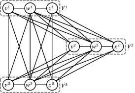
(d) Graph $H$ constructed from $G$.

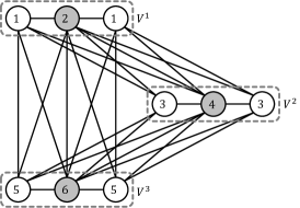
(e) A $k$-coloring $f^{\prime}_{\mathsf{start}}$ of $H$.

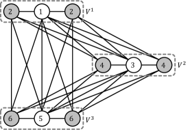
(f) $k$-coloring $f^{\prime}_{\mathsf{end}}$ of $H$.

Figure 1: A failed attempt to reduce Maxmin 2-Cut Reconfiguration to Maxmin $k$-Cut Reconfiguration using [KKLP97]. Given a graph $G$ and its two $2$-colorings $f_{\mathsf{start}},f_{\mathsf{end}}$, we construct a new graph $H$ and its two $k$-colorings $f^{\prime}_{\mathsf{start}},f^{\prime}_{\mathsf{end}}$ according to [KKLP97]. Consider transforming $f^{\prime}_{\mathsf{start}}$ to $f^{\prime}_{\mathsf{end}}$ by recoloring vertices of $V^{1},V^{2},\ldots,V^{\frac{k}{2}}$ in this order. For any intermediate $k$-coloring, (at most) a single induced subgraph $H[V^{i}]$ contains monochromatic edges.

Consider applying the above reduction to reduce Maxmin 2-Cut Reconfiguration to Maxmin $k$-Cut Reconfiguration. Given a graph $G=(V,E)$ and its two proper $2$-colorings $f_{\mathsf{start}},f_{\mathsf{end}}\colon V\to[2]$ as an instance of Maxmin 2-Cut Reconfiguration, we construct an instance $(H,f^{\prime}_{\mathsf{start}},f^{\prime}_{\mathsf{end}})$ of Maxmin $k$-Cut Reconfiguration as follows. Create a new weighted graph $H$ from $G$ according to [KKLP97]. For each $i\in\left[\frac{k}{2}\right]$, we define $V^{i}\coloneq\{v^{i}\mid v\in V\}$. Create then a pair of $k$-colorings $f^{\prime}_{\mathsf{start}},f^{\prime}_{\mathsf{end}}\colon V(H)\to[k]$ of $H$ from $f_{\mathsf{start}},f_{\mathsf{end}}$ such that $f^{\prime}_{\mathsf{start}}(v^{i})\coloneq f_{\mathsf{start}}(v)+2(i-1)$ and $f^{\prime}_{\mathsf{end}}(v^{i})\coloneq f_{\mathsf{end}}(v)+2(i-1)$ for each vertex $v^{i}$ of $H$. See Figures 1b, 1c, 1e and 1f for illustration. Observe that vertices of $V^{i}$ are colored $2i-1$ or $2i$ by both $f^{\prime}_{\mathsf{start}}$ and $f^{\prime}_{\mathsf{end}}$, and every edge of $H$ is bichromatic on $f^{\prime}_{\mathsf{start}}$ and $f^{\prime}_{\mathsf{end}}$. We now show that $\operatorname{\mathsf{opt}}_{H}(f^{\prime}_{\mathsf{start}}\leftrightsquigarrow f^{\prime}_{\mathsf{end}})\geqslant 1-\Theta\left(\tfrac{1}{k^{2}}\right)$ regardless of the value of $\operatorname{\mathsf{opt}}_{G}(f_{\mathsf{start}}\leftrightsquigarrow f_{\mathsf{end}})$. Consider a reconfiguration sequence from $f^{\prime}_{\mathsf{start}}$ to $f^{\prime}_{\mathsf{end}}$ obtained by recoloring vertices of $V^{1},V^{2},\ldots,V^{\frac{k}{2}}$ in this order. Suppose we are on the way of recoloring the vertices of $V^{i}$. Subgraph $H[V^{i}]$ may contain (at most) $|E|$ monochromatic edges, but subgraph $H[V^{j}]$ for any $j\neq i$ contains no monochromatic edges, deriving that

$$\operatorname{\mathsf{opt}}_{H}(f^{\prime}_{\mathsf{start}}\leftrightsquigarrow f^{\prime}_{\mathsf{end}})\geqslant 1-\frac{1\cdot|E|+(\frac{k}{2}-1)\cdot 0}{{k\choose 2}\cdot|E|}\geqslant 1-{k\choose 2}^{-1}=1-\Theta\left(\tfrac{1}{k^{2}}\right).$$ (2.1)

This is undesirable because the ratio between completeness and soundness would be at least $1-\Theta\left(\tfrac{1}{k^{2}}\right)$.

(a) Coloring of $G$ by $f$.

(b) Coloring of $G$ by $g$.

(c) Illustration of $V_{\alpha,\beta}$’s, which partition the vertex set into $k^{2}$ groups.

(d) Coloring of $V_{\alpha,\beta}$’s by $f$, which looks horizontally striped.

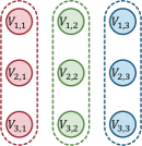
(e) Coloring of $V_{\alpha,\beta}$’s by $g$, which looks vertically striped.

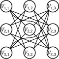
(f) Graph structure of $V_{\alpha,\beta}$’s.

Figure 2: Motivating illustrations for our encoding and stripe test.

Our Reduction Using the Stripe Test.

Our gap-preserving reduction from Maxmin 2-Cut Reconfiguration to Maxmin $k$-Cut Reconfiguration is completely different from those of [KKLP97, GS13]. Briefly speaking, we shall encode a $2$-coloring of each vertex by a $k$-coloring of $[k]^{2}$. Our proposed encoding is motivated by the following scenario: Suppose that for a graph $G=(V,E)$ and its two proper $k$-colorings $f,g\colon V\to[k]$, we would like to transform $f$ into $g$ so as to maximize the minimum fraction of bichromatic edges (see Figures 2a and 2b). For each pair of colors $\alpha,\beta\in[k]$, let $V_{\alpha,\beta}$ be the set of vertices colored $\alpha$ by $f$ and $\beta$ by $g$ (see Figure 2c); namely,

$$V_{\alpha,\beta}\coloneq\Bigl{\{}v\in V\Bigm{|}f(v)=\alpha\text{ and }g(v)=\beta\Bigr{\}}.$$ (2.2)

If $V_{\alpha,\beta}$’s are placed on a $k\times k$ grid, $f$ looks “horizontally striped” while $g$ looks “vertically striped” (see Figures 2d and 2e). Since both $f$ and $g$ are proper, there may exist edges between $V_{\alpha_{1},\beta_{1}}$ and $V_{\alpha_{2},\beta_{2}}$ only if $\alpha_{1}\neq\alpha_{2}$ and $\beta_{1}\neq\beta_{2}$ (see Figure 2f). On the other hand, any transformation from $f$ to $g$ seems to make a significant fraction of edges into monochromatic. The above structural observation motivates the following two ideas:

• (Idea 1) Consider the “striped” pattern represented by a $k$-coloring of $[k]^{2}$ as if it were encoding $[2]$; e.g., the horizontal stripe represents $1$, while the vertical stripe represents $2$. This encoding can be thought of as a very redundant error-correcting code from $[2]$ to $[k]^{k^{2}}$.

• (Idea 2) Check if a $k$-coloring of $[k]^{2}$ is close to a “striped” pattern by executing the following stripe verifier $\mathcal{V}_{\mathrm{stripe}}$, which is allowed to sample a pair from ${[k]^{2}\choose 2}$ probabilistically and accept if they have different colors: [l]Stripe verifier $\mathcal{V}_{\mathrm{stripe}}$.

  1:a $k$-coloring $f\colon[k]^{2}\to[k]$.

  2:select $(x_{1},y_{1})\in[k]^{2}$ and $(x_{2},y_{2})\in[k]^{2}$ s.t. $x_{1}\neq x_{2}$ and $y_{1}\neq y_{2}$ uniformly at random. $f(x_{1},y_{1})=f(x_{2},y_{2})$

  3:declare reject.

  4:declare accept.

  In particular, $\mathcal{V}_{\mathrm{stripe}}$ accepts $f$ with probability $1$ if $f$ is striped.

At the heart of the proof of Lemma 2.1 is the rejection rate of the stripe test, as stated below:

Lemma 2.2 (informal; see Lemma 5.7).

For any $k$-coloring $f\colon[k]^{2}\to[k]$ that is $\varepsilon$-far from being striped, $\mathcal{V}_{\mathrm{stripe}}$ rejects $f$ with probability $\Omega\left(\frac{\varepsilon}{k}\right)$.

The rejection probability “$\Omega\left(\frac{\varepsilon}{k}\right)$” is critical for producing a $\left(1-\Omega\left(\frac{1}{k}\right)\right)$-factor gap between completeness and soundness. The proof of Lemma 2.2 presented in Section 5.4 involves a rather complicated case analysis, exploiting the nontrivial structure of a $k$-coloring of $[k]^{2}$ far from any striped pattern.

For a pair of $k$-colorings $f,g\colon[k]^{2}\to[k]$ sufficiently close to being striped (ensured by Lemma 2.2), we can design the consistency verifier $\mathcal{V}_{\mathrm{cons}}$, which tests if $f$ and $g$ exhibit the same striped pattern. Calling the striped verifier $\mathcal{V}_{\mathrm{stripe}}$ and the consistency verifier $\mathcal{V}_{\mathrm{cons}}$ with a carefully selected probability, we obtain the edge verifier $\mathcal{V}_{\mathrm{edge}}$ with the following properties:

Lemma 2.3 (informal; see Lemmas 5.10 and 5.11).

For any two $k$-colorings $f,g\colon[k]^{2}\to[k]$, the following hold:

• if $f$ and $g$ are exactly striped and exhibit the same striped pattern, $\mathcal{V}_{\mathrm{edge}}$ rejects $f\circ g$ with probability at most $\frac{1}{2Z\cdot k}$;

• if $f$ and $g$ are encoding different striped patterns, $\mathcal{V}_{\mathrm{edge}}$ rejects $f\circ g$ with probability at least $\frac{1}{Z\cdot k}$,

where $Z>0$ is some universal constant.

Given the rejection probability of $\mathcal{V}_{\mathrm{edge}}$, it is easy to reduce Maxmin 2-Cut Reconfiguration to Maxmin $k$-Cut Reconfiguration and prove Lemma 2.1. See Section 5.3 for details.

2.2 Hardness of Approximation for Maxmin E$k$-SAT Reconfiguration

Here, we give a proof overview of Theorem 1.3, i.e., $\PSPACE$-hardness and $\NP$-hardness of approximation for Maxmin E$k$-SAT Reconfiguration. For an E$k$-CNF formula $\varphi$ and its two satisfying assignments $\alpha_{\mathsf{start}},\alpha_{\mathsf{end}}$, let $\operatorname{\mathsf{opt}}_{\varphi}(\alpha_{\mathsf{start}}\leftrightsquigarrow\alpha_{\mathsf{end}})$ denote the optimal value of Maxmin E$k$-SAT Reconfiguration; namely, the maximum of the minimum fraction of satisfied clauses of $\varphi$, where the maximum is taken over all possible reconfiguration sequences from $\alpha_{\mathsf{start}}$ to $\alpha_{\mathsf{end}}$.

Recap of a Simple Reduction.

Before going into the proof details, we first recapitulate a simple reduction from Maxmin E3-SAT Reconfiguration to Maxmin E$k$-SAT Reconfiguration based on that from Max $3$-SAT to Max $k$-SAT, e.g., [Hås01, Theorem 6.14]. Let $\varphi$ be an E$3$-CNF formula consisting of $m$ clauses $C_{1},\ldots,C_{m}$ over $n$ variables $V\coloneq\{x_{1},\ldots,x_{n}\}$, and $\alpha_{\mathsf{start}},\alpha_{\mathsf{end}}\colon V\to\{0,1\}$ be its two satisfying assignments. We construct an instance $(\psi,\alpha^{\prime}_{\mathsf{start}},\alpha^{\prime}_{\mathsf{end}})$ of Maxmin E$k$-SAT Reconfiguration as follows. Create fresh $K$ variables, denoted $y_{1},\ldots,y_{K}$, where $K\coloneq k-3$. Starting from an empty formula $\psi$, for each clause $C_{j}$ of $\varphi$ and each of the $2^{K}$ possible clauses $D$ over $y_{1},\ldots,y_{K}$, add $C_{j}\vee D$ to $\psi$. Define $\alpha^{\prime}_{\mathsf{start}},\alpha^{\prime}_{\mathsf{end}}\colon V\cup\{y_{1},\ldots,y_{K}\}\to\{0,1\}$ such that $\alpha^{\prime}_{\mathsf{start}}|_{V}=\alpha_{\mathsf{start}}$, $\alpha^{\prime}_{\mathsf{start}}|_{\{y_{1},\ldots,y_{K}\}}=0^{K}$, $\alpha^{\prime}_{\mathsf{end}}|_{V}=\alpha_{\mathsf{end}}$, and $\alpha^{\prime}_{\mathsf{end}}|_{\{y_{1},\ldots,y_{K}\}}=0^{K}$, which completes the reduction. Observe easily the following completeness and soundness:

• (Completeness) If $\operatorname{\mathsf{opt}}_{\varphi}(\alpha_{\mathsf{start}}\leftrightsquigarrow\alpha_{\mathsf{end}})=1$, then $\operatorname{\mathsf{opt}}_{\psi}(\alpha^{\prime}_{\mathsf{start}}\leftrightsquigarrow\alpha^{\prime}_{\mathsf{end}})=1$.

• (Soundness) If $\operatorname{\mathsf{opt}}_{\varphi}(\alpha_{\mathsf{start}}\leftrightsquigarrow\alpha_{\mathsf{end}})<1-\varepsilon$, then $\operatorname{\mathsf{opt}}_{\psi}(\alpha^{\prime}_{\mathsf{start}}\leftrightsquigarrow\alpha^{\prime}_{\mathsf{end}})<1-\frac{\varepsilon}{2^{K}}$.

Since Gap_1,1-Ω(1) E3-SAT Reconfiguration is $\PSPACE$-hard [HO24a, KM23, Ohs23], Maxmin E$k$-SAT Reconfiguration is $\PSPACE$-hard to approximate within a factor of $1-\Omega\left(\frac{1}{2^{k}}\right)$. Unfortunately, $1-\Omega\left(\frac{1}{2^{k}}\right)$ (though being optimal for Max E$k$-SAT) is too far from the optimal factor, which lies in $1-\Theta\left(\frac{1}{k}\right)$ due to Theorems 1.3 and 1.4.

To improve the inapproximability factor of $1-\Omega\left(\frac{1}{2^{k}}\right)$, we need to exploit some property that is possessed by Maxmin E$k$-SAT Reconfiguration but not by Max E$k$-SAT. We achieve this by using a “non-monotone” test described next (see Remark 2.4 for the non-monotone property of the test).

$\PSPACE$-hardness Based on the Horn Test.

The crux of closing the chasm between $1-\Omega\left(\frac{1}{2^{k}}\right)$ and $1-\Omega\left(\frac{1}{k}\right)$ is the Horn test. The same as before, let $\varphi$ be an E3-CNF formula consisting of $m$ clauses $C_{1},\ldots,C_{m}$ over $V$, and $\alpha_{\mathsf{start}},\alpha_{\mathsf{end}}\colon V\to\{0,1\}$ be its two satisfying assignments. Let $k\geqslant 6$ be a positive integer divisible by $3$ and $\lambda\coloneq\frac{k}{3}$. The Horn verifier $\mathcal{V}_{\mathrm{Horn}}$, given oracle access to an assignment $\alpha\colon V\to\{0,1\}$, selects $\lambda$ clauses of $\varphi$ randomly, denoted $C_{i_{1}},\ldots,C_{i_{\lambda}}$, and accepts if $\overline{C_{i_{1}}}\vee\cdots\vee\overline{C_{i_{\lambda-1}}}\vee C_{i_{\lambda}}$ is satisfied:

[l]$3\lambda$-query Horn verifier $\mathcal{V}_{\mathrm{Horn}}$ for an E3-CNF formula.

1:an E$3$-CNF formula $\varphi=(C_{1}\vee\cdots\vee C_{m})$ and a positive integer $\lambda\in\mathbb{N}$.

2:an assignment $\alpha\colon V\to\{0,1\}$.

3:sample $i_{1},\ldots,i_{\lambda}\sim[m]$ uniformly at random. $\overline{C_{i_{1}}}\vee\cdots\vee\overline{C_{i_{\lambda-1}}}\vee C_{i_{\lambda}}$ is satisfied by $\alpha$

4:declare accept.

5:declare reject.

Intuitively, the Horn verifier $\mathcal{V}_{\mathrm{Horn}}$ thinks of each clause of $\varphi$ as a new variable and creates a kind of Horn clause on the fly. Observe that if $\alpha$ violates exactly $\varepsilon$-fraction of clauses of $\varphi$, then $\mathcal{V}_{\mathrm{Horn}}$ rejects with probability $\varepsilon(1-\varepsilon)^{\lambda-1}$. Letting $\operatorname{\mathsf{opt}}_{\mathcal{V}_{\mathrm{Horn}}}(\alpha_{\mathsf{start}}\leftrightsquigarrow\alpha_{\mathsf{end}})$ be the maximum of the minimum acceptance probability of $\mathcal{V}_{\mathrm{Horn}}$ over all possible reconfiguration sequences from $\alpha_{\mathsf{start}}$ to $\alpha_{\mathsf{end}}$, we have the following completeness and soundness:

• (Completeness) If $\operatorname{\mathsf{opt}}_{\varphi}(\alpha_{\mathsf{start}}\leftrightsquigarrow\alpha_{\mathsf{end}})=1$, then $\operatorname{\mathsf{opt}}_{\mathcal{V}_{\mathrm{Horn}}}(\alpha_{\mathsf{start}}\leftrightsquigarrow\alpha_{\mathsf{end}})=1$.

• (Soundness) If $\operatorname{\mathsf{opt}}_{\varphi}(\alpha_{\mathsf{start}}\leftrightsquigarrow\alpha_{\mathsf{end}})<1-\varepsilon$, then $\operatorname{\mathsf{opt}}_{\mathcal{V}_{\mathrm{Horn}}}(\alpha_{\mathsf{start}}\leftrightsquigarrow\alpha_{\mathsf{end}})<1-\Omega\left(\frac{\varepsilon}{\lambda}\right)$, given that each variable appears in a constant number of clauses. To see this, we show that any reconfiguration sequence from $\alpha_{\mathsf{start}}$ to $\alpha_{\mathsf{end}}$ contains an assignment $\alpha^{\circ}$ that violates $\approx\frac{\varepsilon}{\lambda}$-fraction of clauses of $\varphi$, which would be rejected by $\mathcal{V}_{\mathrm{Horn}}$ with probability

  $$\Omega\left(\tfrac{\varepsilon}{\lambda}\cdot\left(1-\tfrac{\varepsilon}{\lambda}\right)^{\lambda-1}\right)=\Omega\left(\frac{\varepsilon}{\lambda}\right).$$ (2.3)

Subsequently, we emulate the Horn verifier $\mathcal{V}_{\mathrm{Horn}}$ by an E$k$-CNF formula. Since the negation of any clause $C=(\ell_{1}\vee\ell_{2}\vee\ell_{3})$ can be represented by the following $7$ clauses:

$$\begin{aligned} \overline{C}&=(\overline{\ell_{1}}\vee\ell_{2}\vee\ell_{3})\wedge(\ell_{1}\vee\overline{\ell_{2}}\vee\ell_{3})\wedge(\ell_{1}\vee\ell_{2}\vee\overline{\ell_{3}})\\ &\qquad\wedge(\ell_{1}\vee\overline{\ell_{2}}\vee\overline{\ell_{3}})\wedge(\overline{\ell_{1}}\vee\ell_{2}\vee\overline{\ell_{3}})\wedge(\overline{\ell_{1}}\vee\overline{\ell_{2}}\vee\ell_{3})\wedge(\overline{\ell_{1}}\vee\overline{\ell_{2}}\vee\overline{\ell_{3}}),\end{aligned}$$ (2.4)

each acceptance condition of $\mathcal{V}_{\mathrm{Horn}}$, i.e., $\overline{C_{i_{1}}}\vee\cdots\vee\overline{C_{i_{\lambda-1}}}\vee C_{i_{\lambda}}$, can be represented by an E$(3\lambda)$-CNF formula consisting of $7^{\lambda-1}$ clauses. Constructing an E$k$-CNF formula $\psi$ that simulates $\mathcal{V}_{\mathrm{Horn}}$, we obtain a new instance $(\psi,\alpha_{\mathsf{start}},\alpha_{\mathsf{end}})$ of Maxmin E$k$-SAT Reconfiguration, which exhibits the following completeness and soundness:

• (Completeness) If $\operatorname{\mathsf{opt}}_{\varphi}(\alpha_{\mathsf{start}}\leftrightsquigarrow\alpha_{\mathsf{end}})=1$, then $\operatorname{\mathsf{opt}}_{\psi}(\alpha_{\mathsf{start}}\leftrightsquigarrow\alpha_{\mathsf{end}})=1$.

• (Soundness) If $\operatorname{\mathsf{opt}}_{\varphi}(\alpha_{\mathsf{start}}\leftrightsquigarrow\alpha_{\mathsf{end}})<1-\varepsilon$, then $\operatorname{\mathsf{opt}}_{\psi}(\alpha_{\mathsf{start}}\leftrightsquigarrow\alpha_{\mathsf{end}})<1-\Omega\left(\frac{\varepsilon}{1.913^{k}}\right)$. Let $\alpha^{\circ}\colon V\to\{0,1\}$ be an assignment that violates $\Theta\left(\frac{\varepsilon}{\lambda}\right)$-fraction of clauses of $\varphi$. Suppose $\mathcal{V}_{\mathrm{Horn}}$ rejects $\alpha^{\circ}$ when examining the condition $\overline{C_{i_{1}}}\vee\cdots\vee\overline{C_{i_{\lambda-1}}}\vee C_{i_{\lambda}}$. By construction of $\psi$, exactly one of the $7^{\lambda-1}$ clauses (which emulate $\overline{C_{i_{1}}}\vee\cdots\vee\overline{C_{i_{\lambda-1}}}\vee C_{i_{\lambda}}$) must be violated by $\alpha^{\circ}$. Therefore, the fraction of clauses of $\psi$ violated by $\alpha^{\circ}$ is

  $$\underbrace{\operatorname*{\mathbb{P}}\Bigl{[}\mathcal{V}_{\mathrm{Horn}}\text{ rejects }\alpha^{\circ}\Bigr{]}}_{=\Omega\left(\frac{\varepsilon}{\lambda}\right)}\cdot\frac{1}{7^{\lambda-1}}=\Omega\left(\frac{\varepsilon}{k\cdot 7^{\frac{1}{3}k}}\right)\underbrace{=}_{7^{\frac{1}{3}}<1.913}\Omega\left(\frac{\varepsilon}{1.913^{k}}\right).$$ (2.5)

Consequently, Maxmin E$k$-SAT Reconfiguration is $\PSPACE$-hard to approximate within a factor of $1-\Omega\left(\frac{1}{1.913^{k}}\right)$, which is an exponential improvement over $1-\Omega\left(\frac{1}{2^{k}}\right)$. Constructing $\mathcal{V}_{\mathrm{Horn}}$ from a PCRP verifier with query complexity $\Theta(\sqrt{k})$ and free-bit complexity $\log_{2}5\approx 2.32$, we can further improve the inapproximability factor to $1-\Omega\left(\frac{1}{9^{\sqrt{k}}}\right)$. See Section 7.1 for the details.

Remark 2.4 (Why is the Horn test not applicable to Max E$k$-SAT?).

One may wonder if the Horn verifier $\mathcal{V}_{\mathrm{Horn}}$ can be used to reduce Max E3-SAT to Max E$k$-SAT to derive $\NP$-hardness of approximation within a factor of $1-\Omega\left(\frac{1}{1.913^{k}}\right)$, which contradicts the fact that Max E$k$-SAT is $\left(1-\frac{1}{2^{k}}\right)$-factor approximable [Joh74]. This idea dose not work for the following reason: Given an assignment that violates exactly $\varepsilon$-fraction of clauses, $\mathcal{V}_{\mathrm{Horn}}$ rejects with probability equal to $\varepsilon(1-\varepsilon)^{\lambda-1}$, which is not monotone with respect to $\varepsilon$; in particular, $\varepsilon(1-\varepsilon)^{\lambda-1}$ approaches $0$ as $\varepsilon\to 1$. Therefore, even in the soundness case of Gap${}_{1,1-\varepsilon_{0}}$ E3-SAT, $\mathcal{V}_{\mathrm{Horn}}$ may accept some assignment (though making most of the clauses unsatisfied) with probability close to $1$. On the other hand, in the soundness case of Gap${}_{1,1-\varepsilon_{0}}$ E3-SAT Reconfiguration, every reconfiguration sequence contains some assignment that violates $\Theta\left(\frac{\varepsilon_{0}}{\lambda}\right)$-fraction of clauses, which would be rejected by $\mathcal{V}_{\mathrm{Horn}}$ with probability $\Omega\left(\frac{\varepsilon_{0}}{\lambda}\right)$, so that the maximum rejection probability of $\mathcal{V}_{\mathrm{Horn}}$ is $\Omega\left(\frac{\varepsilon_{0}}{\lambda}\right)$ too. See also Figure 3 for illustration. In this sense, the Horn verifier is specially tailored to reconfiguration problems.

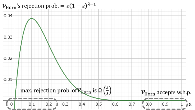
Figure 3: The rejection probability of the Horn verifier $\mathcal{V}_{\mathrm{Horn}}$ parameterized by $\varepsilon$, the fraction of violated clauses. Since the rejection probability $\varepsilon(1-\varepsilon)^{\lambda-1}$ is not monotone, in the soundness case of Gap${}_{1,1-\varepsilon_{0}}$ E3-SAT, $\mathcal{V}_{\mathrm{Horn}}$ may accept some assignment with high probability. On the other hand, in the soundness case of Gap${}_{1,1-\varepsilon_{0}}$ E$k$-SAT Reconfiguration, every reconfiguration sequence must contain some assignment that violates a $\Theta\left(\frac{\varepsilon_{0}}{\lambda}\right)$-fraction of clauses, so that $\mathcal{V}_{\mathrm{Horn}}$’s maximum rejection probability is $\Omega\left(\frac{\varepsilon_{0}}{\lambda}\right)$.

Asymptotically Tight $\NP$-hardness.

The proof of asymptotically tight $\NP$-hardness uses a gap-preserving reduction from Gap_1,1-ε E3-SAT to Gap${}_{1,1-\frac{\varepsilon}{k-3}}$ E$k$-SAT Reconfiguration, which is simpler than that for $\PSPACE$-hardness. Given an E3-CNF formula $\varphi$ consisting of $m$ clauses $C_{1},\ldots,C_{m}$ over $n$ variables $x_{1},\ldots,x_{n}$, we construct an instance $(\psi,\alpha_{\mathsf{start}},\alpha_{\mathsf{end}})$ of Maxmin E$k$-SAT Reconfiguration for $k\geqslant 5$ as follows: Create $K$ fresh variables, denoted $y_{1},\ldots,y_{K}$, where $K\coloneq k-3$. Starting from an empty formula $\psi$, for each clause $C_{j}$ of $\varphi$ and each of the $K$ possible Horn clauses, $H_{i}\coloneq(y_{i}\vee\bigvee_{i^{\prime}\neq i}\overline{y_{i^{\prime}}})$, over $y_{1},\ldots,y_{K}$, add $C_{j}\vee H_{i}$ to $\psi$. Define $\alpha_{\mathsf{start}}\coloneq 1^{n+K}$ and $\alpha_{\mathsf{end}}\coloneq 0^{n+K}$, both of which satisfy $\psi$. The completeness is immediate by construction. The soundness claims that if every possible assignment violates more than $\delta$-fraction of clauses of $\varphi$, then $\operatorname{\mathsf{opt}}_{\psi}(\alpha_{\mathsf{start}}\leftrightsquigarrow\alpha_{\mathsf{end}})<1-\frac{\delta}{K}$. The proof is based on the following fact: Any reconfiguration sequence from $\alpha_{\mathsf{start}}$ to $\alpha_{\mathsf{end}}$ contains an assignment $\alpha^{\circ}$ such that $\alpha^{\circ}|_{\{y_{1},\ldots,y_{K}\}}$ contains a single $0$. Thus, for each clause $C_{j}$ unsatisfied by $\alpha^{\circ}|_{\{x_{1},\ldots,x_{n}\}}$, $\alpha^{\circ}$ does not satisfy exactly one clause in the form of $C_{j}\vee H_{i}$, which implies the soundness.

Since the above reduction does not work when $k\leqslant 4$, we give a gap-preserving reduction from Max E3-SAT to Maxmin E3-SAT Reconfiguration and Maxmin E4-SAT Reconfiguration separately, which are obtained by modifying [IDHPSUU11, Theorem 5]. See Appendix B for details.

We conclude this subsection with a simple yet interesting example of Maxmin E3-SAT Reconfiguration, demonstrating the “numerical” difference from Max E3-SAT.

Example 2.5.

Consider the following instance of Maxmin E3-SAT Reconfiguration: For a positive integer $n$ divisible by $3$, let $x_{1},\ldots,x_{n}$ be $n$ variables and $\varphi$ be an E$3$-CNF formula consisting of all possible Horn clauses of size $3$ over $x_{1},\ldots,x_{n}$; namely, for each triple $\{i,j,k\}\in\binom{n}{3}$, $\varphi$ contains the three Horn clauses $(x_{i}\vee\overline{x_{j}}\vee\overline{x_{k}})$, $(\overline{x_{i}}\vee x_{j}\vee\overline{x_{k}})$, and $(\overline{x_{i}}\vee\overline{x_{j}}\vee x_{k})$. Define $\alpha_{\mathsf{start}}=0^{n}$ and $\alpha_{\mathsf{end}}=1^{n}$, both of which satisfy $\varphi$. Consider any reconfiguration sequence $\mathscr{A}=(\alpha^{(1)},\ldots,\alpha^{(T)})$ from $\alpha_{\mathsf{start}}$ to $\alpha_{\mathsf{end}}$. For each $0\leqslant k\leqslant n$, there must be an assignment $\alpha^{\circ}$ in $\mathscr{A}$ that contains exactly $k$ $1$’s. Each Horn clause $(x_{i}\vee\overline{x_{j}}\vee\overline{x_{k}})$ would be violated by $\alpha^{\circ}$ if and only if $\alpha^{\circ}(x_{i})=0$, $\alpha^{\circ}(x_{j})=1$, and $\alpha^{\circ}(x_{k})=1$; thus, there are $\binom{k}{2}\cdot(n-k)$ of such violated clauses. Setting $k\coloneq\frac{2}{3}n$, the fraction of clauses violated by $\alpha^{\circ}$ is

$$\frac{\binom{k}{2}\cdot(n-k)}{3\cdot\binom{n}{3}}=\frac{\frac{2}{27}\cdot n^{2}\left(n-\tfrac{3}{2}\right)}{\frac{1}{2}\cdot n(n-1)(n-2)}>\frac{4}{27}.$$ (2.6)

Consequently, any reconfiguration sequence for this instance cannot satisfy $\frac{23}{27}$-fraction of clauses. On the other hand, at least $\frac{7}{8}$-fraction of clauses can be satisfied for any Max E3-SAT instance. Since $\frac{23}{27}=0.\dot{8}\dot{5}\dot{1}<0.875=\frac{7}{8}$, Maxmin E3-SAT Reconfiguration seems “harder” than Max E3-SAT.

2.3 Approximation Algorithms for Maxmin $k$-Cut Reconfiguration and Maxmin E$k$-SAT Reconfiguration

We present a highlight of approximation algorithms for Maxmin $k$-Cut Reconfiguration and Maxmin E$k$-SAT Reconfiguration (Theorems 1.2 and 1.4). Our proposed algorithms share a common methodology, that is, a random reconfiguration via a random solution. Here, we sketch a $\left(1-\frac{2}{k}\right)$-factor approximation algorithm for Maxmin $k$-Cut Reconfiguration. Let $G$ be a graph and $f_{\mathsf{start}},f_{\mathsf{end}}$ be its proper $k$-colorings (for the sake of simplicity). We say that a vertex of $G$ is low degree if its degree is less than $|E(G)|^{\frac{2}{3}}$, and high degree otherwise. Suppose first $G$ only contains low-degree vertices. Let $F$ be a random $k$-coloring of $G$, which makes $\left(1-\frac{1}{k}\right)$-fraction of edges bichromatic in expectation. Consider a random reconfiguration sequence $\mathscr{F}$ from $f_{\mathsf{start}}$ to $F$ obtained by recoloring vertices at which $f_{\mathsf{start}}$ and $F$ differ in a random order. It is easy to see that each edge of $G$ is always bichromatic through $\mathscr{F}$ with probability at least $\left(1-\frac{1}{k}\right)^{2}=1-\frac{2}{k}+\frac{1}{k^{2}}$. By the read-$k$ Chernoff bound [GLSS15] with $k=|E(G)|^{\frac{2}{3}}$, with high probability, any intermediate $k$-coloring of $\mathscr{F}$ makes $\left(1-\frac{2}{k}\right)$-fraction of edges bichromatic. Concatenating a random reconfiguration sequence from $F$ to $f_{\mathsf{end}}$ to $\mathscr{F}$, we obtain a random reconfiguration sequence from $f_{\mathsf{start}}$ to $f_{\mathsf{end}}$ having the desired property (with high probability). To deal with high-degree vertices, we use the following ad-hoc observations:

• Since there are few high-degree vertices, the number of edges between them is negligible.

• Each high-degree vertex has “many” low-degree neighbors, whose $k$-coloring by $F$ is distributed almost evenly; thus, $\approx\left(1-\frac{1}{k}\right)$-fraction of edges between them are bichromatic with high probability.

See Section 6 for the details. Derandomization can be done by the method of conditional expectations [AS16].

The proposed algorithm for Maxmin E$k$-SAT Reconfiguration works as follows: Given an E$k$-CNF formula $\varphi$ and its two satisfying assignments $\alpha_{\mathsf{start}},\alpha_{\mathsf{end}}$, we create a random assignment $A$, a reconfiguration sequence $\mathscr{A}_{1}$ from $\alpha_{\mathsf{start}}$ to $A$ by flipping the assignment to variables at which $\alpha_{\mathsf{start}}$ and $A$ disagree in a random order, and a reconfiguration sequence $\mathscr{A}_{2}$ from $A$ to $\alpha_{\mathsf{end}}$ by flipping the assignment to variables at which $A$ and $\alpha_{\mathsf{end}}$ disagree in a random order. We show that any clause of $\varphi$ remains satisfied throughout $\mathscr{A}_{1}\circ\mathscr{A}_{2}$ with probability at least $1-\frac{2.5}{k}$.

3 Related Work

Hardness of Approximation for Reconfiguration Problems.

[IDHPSUU11] showed that Maxmin 5-SAT Reconfiguration and Maxmin Clique Reconfiguration are $\NP$-hard to approximate, relying on $\NP$-hardness of approximating Max 3-SAT [Hås01] and Max Clique [Hås99], respectively. [KM23] proved -hardness of $\left(\frac{1}{2}+\varepsilon\right)$-factor approximation for Maxmin 2-CSP Reconfiguration and $(2-\varepsilon)$-factor approximation for Minmax Set Cover Reconfiguration for every $\varepsilon>0$, which is numerically tight given matching upper bounds [KM23, IDHPSUU11]. Note that the above $\NP$-hardness results are not optimal in a sense that these reconfiguration problems are actually $\PSPACE$-hard to approximate.

Toward $\PSPACE$-hardness of approximation for reconfiguration problems, [Ohs23] postulated the Reconfiguration Inapproximability Hypothesis (RIH) as a reconfiguration analogue of the PCP theorem [AS98, ALMSS98], and demonstrated $\PSPACE$-hardness of approximation for many popular reconfiguration problems, including those of 3-SAT, Independent Set, Vertex Cover, Clique, Dominating Set, and Set Cover. Recently, RIH has been proven by [HO24a] and [KM23] independently, implying that [Ohs23]’s $\PSPACE$-hardness results hold unconditionally.

In $\NP$ optimization problems, the parallel repetition theorem of [Raz98] can be used to derive explicit, strong inapproximability results. Unfortunately, a naive parallel repetition does not work for reconfiguration problems [Ohs23a]. [Ohs24] took a different approach and adapted [Din07]’s gap amplification [Din07, Rad06, RS07], showing that Maxmin 2-CSP Reconfiguration and Minmax Set Cover Reconfiguration are $\PSPACE$-hard to approximate within a factor of $0.9942$ and $1.0029$, respectively. Subsequently, [HO24] demonstrated that Minmax Set Cover Reconfiguration (and Minmax Dominating Set Reconfiguration) is $\PSPACE$-hard to approximate within a factor of $2-o(1)$, improving upon [KM23, Ohs24]. This is the first optimal $\PSPACE$-hardness result for approximability of any reconfiguration problem.

Approximation Algorithms for Reconfiguration Problems.

Other reconfiguration problems for which approximation algorithms were developed include Minmax Set Cover Reconfiguration, which admits a $2$-factor approximation [IDHPSUU11], Maxmin 2-CSP Reconfiguration, which admits a $\left(\frac{1}{2}-\varepsilon\right)$-factor approximation [KM23], Subset Sum Reconfiguration, which admits a PTAS [ID14], and Submodular Reconfiguration, which admits a constant-factor approximation [OM22]. Note that [KM23] construct a reconfiguration sequence using a random assignment to approximate Maxmin 2-CSP Reconfiguration.

Other Optimization Variants of Reconfiguration Problems.

We note that optimization variants of reconfiguration problems frequently refer to those of the shortest reconfiguration sequence [MNPR17, BHIKMMSW20, IKKKO22, KMM11], which are orthogonal to this study.

4 Preliminaries

For a nonnegative integer $n\in\mathbb{N}$, let $[n]\coloneq\{1,2,\ldots,n\}$. We use the Iverson bracket; i.e., for a statement $P$, $\llbracket P\rrbracket$ is equal to $1$ if $P$ is true and $0$ otherwise. A sequence $\mathscr{S}$ of a finite number of objects, $s^{(1)},\ldots,s^{(T)}$, is denoted by $(s^{(1)},\ldots,s^{(T)})$, and we write $s\in\mathscr{S}$ to indicate that $s$ appears in $\mathscr{S}$. The symbol $\circ$ stands for a concatenation of two sequences or functions. For a set $\mathcal{S}$, $X\sim\mathcal{S}$ means that $X$ is a random variable uniformly sampled from $\mathcal{S}$.

For a function $f\colon\mathcal{D}\to\mathcal{R}$ over a finite domain $\mathcal{D}$ and a subset $\mathcal{S}\subseteq\mathcal{D}$, we use $f|_{\mathcal{S}}\colon\mathcal{S}\to\mathcal{R}$ to denote the restriction of $f$ to $\mathcal{S}$. For two functions $f,g\colon\mathcal{D}\to\mathcal{R}$ over a finite domain $\mathcal{D}$, the relative Hamming distance between $f$ and $g$, denoted by $\operatorname{\mathsf{dist}}(f,g)$, is defined as the fraction of positions of $\mathcal{D}$ at which $f$ and $g$ differ; namely,

$$\operatorname{\mathsf{dist}}(f,g)\coloneq\operatorname*{\mathbb{P}}_{x\sim\mathcal{D}}\Bigl{[}f(x)\neq g(x)\Bigr{]}=|\mathcal{D}|^{-1}\cdot\left|\Bigl{\{}x\in\mathcal{D}\Bigm{|}f(x)\neq g(x)\Bigr{\}}\right|.$$ (4.1)

We say that $f$ is $\varepsilon$-close to $g$ if $\operatorname{\mathsf{dist}}(f,g)\leqslant\varepsilon$ and $\varepsilon$-far if $\operatorname{\mathsf{dist}}(f,g)>\varepsilon$. Similar notations are used for a set of function $G$ from $\mathcal{D}$ to $\mathcal{R}$; e.g., $\operatorname{\mathsf{dist}}(f,G)\coloneq\min_{g\in G}\operatorname{\mathsf{dist}}(f,g)$ and $f$ is $\varepsilon$-close to $G$ if $\operatorname{\mathsf{dist}}(f,G)\leqslant\varepsilon$.

4.1 Max $k$-Cut and Maxmin $k$-Cut Reconfiguration

We formulate $k$-Coloring Reconfiguration and its optimization variant. Throughout this paper, all graphs are undirected. For a graph $G=(V,E)$, let $V(G)$ and $E(G)$ denote the vertex set and edge set of $G$, respectively. For a vertex $v$ of $G$, let $\mathcal{N}_{G}(v)$ denote the set of neighbors of $v$ and $d_{G}(v)$ denote the degree of $v$. For a vertex set $S\subseteq V(G)$, we write $G[S]$ for the subgraph of $G$ induced by $S$. Unless otherwise stated, graphs appearing in this paper are multigraphs; namely, the edge set is a multiset consisting of parallel edges.

For a graph $G=(V,E)$ and a positive integer $k\in\mathbb{N}$, a $k$-coloring of $G$ is a function $f\colon V\to[k]$ that assigns a color of $[k]$ to each vertex of $G$. We call $f(v)$ the color of $v$. Edge $(v,w)$ of $G$ is said to be bichromatic on $f$ if $f(v)\neq f(w)$ and monochromatic on $f$ if $f(v)=f(w)$. We say that a $k$-coloring $f$ of $G$ is proper if it makes every edge of $G$ bichromatic. The value of $f$ is defined as the fraction of edges of $G$ made bichromatic by $f$; namely,

$$\operatorname{\mathsf{val}}_{G}(f)\coloneq\frac{1}{|E|}\cdot\left|\Bigl{\{}(v,w)\in E\Bigm{|}f(v)\neq f(w)\Bigr{\}}\right|.$$ (4.2)

Recall that for a graph $G$, $k$-Coloring asks to decide if there is a proper $k$-coloring $f$ of $G$, and its optimization version called Max $k$-Cut (a.k.a. Max $k$-Colorable Subgraph [PY91, GS13]) requires to find a $k$-coloring $f$ of $G$ that maximizes $\operatorname{\mathsf{val}}_{G}(f)$.

Subsequently, we formulate a reconfiguration version of $k$-Coloring as well as Max $k$-Cut. For a graph $G=(V,E)$ and its two $k$-colorings $f_{\mathsf{start}},f_{\mathsf{end}}\colon V\to[k]$, a reconfiguration sequence from $f_{\mathsf{start}}$ to $f_{\mathsf{end}}$ is any sequence $\mathscr{F}=(f^{(1)},\ldots,f^{(T)})$ over $k$-colorings of $G$ such that $f^{(1)}=f_{\mathsf{start}}$, $f^{(T)}=f_{\mathsf{end}}$, and every pair of adjacent $k$-colorings differs in at most one vertex. The $k$-Coloring Reconfiguration problem [BC09, CvJ11, CvJ08, CvJ09] asks to decide if there is a reconfiguration sequence from $f_{\mathsf{start}}$ to $f_{\mathsf{end}}$ consisting only of proper $k$-colorings of $G$. Note that $k$-Coloring Reconfiguration is polynomial-time solvable if $k\leqslant 3$ [CvJ11] while it becomes $\PSPACE$-complete for every $k\geqslant 4$ [BC09].

Since we are concerned with approximability of $k$-Cut Reconfiguration, we formulate its optimization variant. For a reconfiguration sequence $\mathscr{F}=(f^{(1)},\ldots,f^{(T)})$ over $k$-colorings of $G$, let $\operatorname{\mathsf{val}}_{G}(\mathscr{F})$ denote the minimum fraction of bichromatic edges over all $f^{(t)}$’s in $\mathscr{F}$; namely,

$$\operatorname{\mathsf{val}}_{G}(\mathscr{F})\coloneq\min_{f^{(t)}\in\mathscr{F}}\operatorname{\mathsf{val}}_{G}(f^{(t)}).$$ (4.3)

For a graph $G=(V,E)$ and its two $k$-colorings $f_{\mathsf{start}},f_{\mathsf{end}}$, Maxmin $k$-Cut Reconfiguration requires to maximize $\operatorname{\mathsf{val}}_{G}(\mathscr{F})$ subject to $\mathscr{F}=(f_{\mathsf{start}},\ldots,f_{\mathsf{end}})$. Maxmin $k$-Cut Reconfiguration is $\PSPACE$-hard because so is $k$-Coloring Reconfiguration. For two $k$-colorings $f_{\mathsf{start}},f_{\mathsf{end}}$ of $G$, let $\operatorname{\mathsf{opt}}_{G}(f_{\mathsf{start}}\leftrightsquigarrow f_{\mathsf{end}})$ denote the maximum value of $\operatorname{\mathsf{val}}_{G}(\mathscr{F})$ over all possible reconfiguration sequences $\mathscr{F}$ from $f_{\mathsf{start}}$ to $f_{\mathsf{end}}$; namely,

$$\operatorname{\mathsf{opt}}_{G}(f_{\mathsf{start}}\leftrightsquigarrow f_{\mathsf{end}})\coloneq\max_{\mathscr{F}=(f_{\mathsf{start}},\ldots,f_{\mathsf{end}})}\operatorname{\mathsf{val}}_{G}(\mathscr{F}).$$ (4.4)

Note that $\operatorname{\mathsf{opt}}_{G}(f_{\mathsf{start}}\leftrightsquigarrow f_{\mathsf{end}})\leqslant\min\{\operatorname{\mathsf{val}}_{G}(f_{\mathsf{start}}),\operatorname{\mathsf{val}}_{G}(f_{\mathsf{end}})\}$. The gap version of Maxmin $k$-Cut Reconfiguration is defined as follows.

Problem 4.1.

For every numbers $0\leqslant s\leqslant c\leqslant 1$ and positive integer $k\in\mathbb{N}$, Gap_c,s $k$-Cut Reconfiguration requires to determine for a graph $G$ and its two $k$-colorings $f_{\mathsf{start}},f_{\mathsf{end}}$, whether $\operatorname{\mathsf{opt}}_{G}(f_{\mathsf{start}}\leftrightsquigarrow f_{\mathsf{end}})\geqslant c$ or $\operatorname{\mathsf{opt}}_{G}(f_{\mathsf{start}}\leftrightsquigarrow f_{\mathsf{end}})<s$. Here, $c$ and $s$ are respectively called completeness and soundness.

We say that a reconfiguration sequence $\mathscr{F}=(f^{(1)},\ldots,f^{(T)})$ from $f_{\mathsf{start}}$ to $f_{\mathsf{end}}$ is irredundant if no pair of adjacent $k$-colorings are identical, and for each vertex $v$ of $G$, there is index $t^{*}\in[T]$ such that $f^{(t)}(v)$ is $f_{\mathsf{start}}(v)$ if $t\leqslant t^{*}$ and $f_{\mathsf{end}}(v)$ otherwise. Informally, irredundancy ensures that each vertex is recolored at most once; in particular, the length of $\mathscr{F}$ must be the number of vertices on which $f_{\mathsf{start}}$ and $f_{\mathsf{end}}$ differ. Let $\mathbb{F}(f_{\mathsf{start}}\leftrightsquigarrow f_{\mathsf{end}})$ denote the set of all irredundant reconfiguration sequences from $f_{\mathsf{start}}$ to $f_{\mathsf{end}}$. The size of $\mathbb{F}(f_{\mathsf{start}}\leftrightsquigarrow f_{\mathsf{end}})$ is equal to $d!$, where $d$ is the number of vertices on which $f_{\mathsf{start}}$ and $f_{\mathsf{end}}$ differ. For any $\ell$ $k$-colorings $f_{1},f_{2},\ldots,f_{\ell}$ of a graph $G$, let $\mathbb{F}(f_{1}\leftrightsquigarrow f_{2}\leftrightsquigarrow\cdots\leftrightsquigarrow f_{\ell})$ denote the set of reconfiguration sequences obtained by concatenating any $\ell-1$ irredundant reconfiguration sequences of $\mathbb{F}(f_{i}\leftrightsquigarrow f_{i+1})$ for all $i\in[\ell-1]$, which can be defined recursively as follows:

$$\mathbb{F}(f_{1}\leftrightsquigarrow f_{2}\leftrightsquigarrow\cdots\leftrightsquigarrow f_{\ell})\coloneq\Bigl{\{}\mathscr{F}\circ\mathscr{F}^{\prime}\Bigm{|}\mathscr{F}\in\mathbb{F}(f_{1}\leftrightsquigarrow f_{2})\text{ and }\mathscr{F}^{\prime}\in\mathbb{F}(f_{2}\leftrightsquigarrow\cdots\leftrightsquigarrow f_{\ell})\Bigr{\}}.$$ (4.5)

4.2 Max $k$-SAT and Maxmin E$k$-SAT Reconfiguration

We formulate E$k$-SAT Reconfiguration and its optimization variant. We use the standard terminology and notation of Boolean satisfiability. Truth values are denoted by $1$ (true) or $0$ (false). A Boolean formula $\varphi$ consists of Boolean variables $x_{1},\ldots,x_{n}$ and the logical operators, And ($\wedge$), Or ($\vee$), and Not ($\neg$). An assignment for $\varphi$ is a mapping $\alpha\colon\{x_{1},\ldots,x_{n}\}\to\{0,1\}$ that assigns a truth value to each variable. A Boolean formula $\varphi$ is said to be satisfiable if there exists an assignment $\alpha$ such that $\varphi$ evaluates to $1$ when each variable $x_{i}$ is assigned the truth value specified by $\alpha(x_{i})$. A literal is either a variable or its negation, and a clause is a disjunction of literals. A Boolean formula is in conjunctive normal form (CNF) if it is a conjunction of clauses. By abuse of notation, for an assignment $\alpha\colon\{x_{1},\ldots,x_{n}\}\to\{0,1\}$ and a negative literal $\overline{x_{i}}$, we write $\alpha(\overline{x_{i}})\coloneq\overline{\alpha(x_{i})}$. A $k$-CNF formula is a CNF formula of which every clause contains at most $k$ literals. The prefix “E$k$-” means that every clause contains exactly $k$ literals of distinct variables. For a CNF formula $\varphi$ consisting of $m$ clauses $C_{1},\ldots,C_{m}$, the value of an assignment $\alpha$ for $\varphi$ is defined as the fraction of clauses of $\varphi$ satisfied by $\alpha$; namely,

$$\operatorname{\mathsf{val}}_{\varphi}(\alpha)\coloneq\frac{1}{m}\cdot\left|\Bigl{\{}j\in[m]\Bigm{|}\alpha\text{ satisfies }C_{j}\Bigr{\}}\right|.$$ (4.6)

Recall that Max $k$-SAT requires to find an assignment $\alpha$ that maximizes $\operatorname{\mathsf{val}}_{\varphi}(\alpha)$.

We proceed to a reconfiguration version of Max $k$-SAT. For a CNF formula $\varphi$ over $n$ variables $V\coloneq\{x_{1},\ldots,x_{n}\}$ and its two assignments $\alpha_{\mathsf{start}},\alpha_{\mathsf{end}}\colon V\to\{0,1\}$, a reconfiguration sequence from $\alpha_{\mathsf{start}}$ to $\alpha_{\mathsf{end}}$ is any sequence $\mathscr{A}=(\alpha^{(1)},\ldots,\alpha^{(T)})$ overs assignments for $\varphi$ such that $\alpha^{(1)}=\alpha_{\mathsf{start}}$, $\alpha^{(T)}=\alpha_{\mathsf{end}}$, and every pair of adjacent assignments differs in at most one variable. The E$k$-SAT Reconfiguration problem [GKMP09] requires to determine for an E$k$-CNF formula $\varphi$ and its two satisfying assignments $\alpha_{\mathsf{start}},\alpha_{\mathsf{end}}$, whether there is a reconfiguration sequence from $\alpha_{\mathsf{start}}$ to $\alpha_{\mathsf{end}}$ consisting only of satisfying assignments for $\varphi$. E$k$-SAT Reconfiguration is $\PSPACE$-complete for every $k\geqslant 3$ [GKMP09]. We say that a reconfiguration sequence $\mathscr{A}=(\alpha^{(1)},\ldots,\alpha^{(T)})$ satisfies a clause $C$ if every assignment $\alpha^{(t)}$ of $\mathscr{A}$ satisfies $C$. For a reconfiguration sequence $\mathscr{A}$ of assignments for $\varphi$, let $\operatorname{\mathsf{val}}_{\varphi}(\mathscr{A})$ denote the minimum fraction of satisfied clauses of $\varphi$ over all $\alpha^{(t)}$’s in $\mathscr{A}$; namely,

$$\operatorname{\mathsf{val}}_{\varphi}(\mathscr{A})\coloneq\min_{\alpha^{(t)}\in\mathscr{A}}\operatorname{\mathsf{val}}_{\varphi}(\alpha^{(t)}).$$ (4.7)

Then, Maxmin E$k$-SAT Reconfiguration requests to maximize $\operatorname{\mathsf{val}}_{\varphi}(\mathscr{A})$ subject to $\mathscr{A}=(\alpha_{\mathsf{start}},\ldots,\alpha_{\mathsf{end}})$. For two assignments $\alpha_{\mathsf{start}},\alpha_{\mathsf{end}}$ for $\varphi$, let $\operatorname{\mathsf{opt}}_{\varphi}(\alpha_{\mathsf{start}}\leftrightsquigarrow\alpha_{\mathsf{end}})$ denote the maximum value of $\operatorname{\mathsf{val}}_{\varphi}(\mathscr{A})$ over all possible reconfiguration sequences $\mathscr{A}$ from $\alpha_{\mathsf{start}}$ to $\alpha_{\mathsf{end}}$; namely,

$$\operatorname{\mathsf{opt}}_{\varphi}(\alpha_{\mathsf{start}}\leftrightsquigarrow\alpha_{\mathsf{end}})\coloneq\max_{\mathscr{A}=(\alpha_{\mathsf{start}},\ldots,\alpha_{\mathsf{end}})}\operatorname{\mathsf{val}}_{\varphi}(\mathscr{A}).$$ (4.8)

The gap version of Maxmin E$k$-SAT Reconfiguration is defined as follows.

Problem 4.2.

For every numbers $0\leqslant s\leqslant c\leqslant 1$ and positive integer $k\in\mathbb{N}$, Gap_c,s E$k$-SAT Reconfiguration requires to determine for an E$k$-CNF formula $\varphi$ and its satisfying assignments $\alpha_{\mathsf{start}},\alpha_{\mathsf{end}}$, whether $\operatorname{\mathsf{opt}}_{\varphi}(\alpha_{\mathsf{start}}\leftrightsquigarrow\alpha_{\mathsf{end}})\geqslant c$ or $\operatorname{\mathsf{opt}}_{\varphi}(\alpha_{\mathsf{start}}\leftrightsquigarrow\alpha_{\mathsf{end}})<s$.

Note that the case of $s=c=1$ particularly reduces to E$k$-SAT Reconfiguration.

For two assignments $\alpha_{1},\alpha_{2}\colon\{x_{1},\ldots,x_{n}\}\to\{0,1\}$, we define $\alpha_{1}\triangle\alpha_{2}$ as the set of variables at which $\alpha_{1}$ and $\alpha_{2}$ differ; namely,

$$\alpha_{1}\triangle\alpha_{2}\coloneq\Bigl{\{}x_{i}\Bigm{|}\alpha_{1}(x_{i})\neq\alpha_{2}(x_{i})\Bigr{\}}.$$ (4.9)

We say that a reconfiguration sequence $\mathscr{A}=(\alpha^{(1)},\ldots,\alpha^{(T)})$ from $\alpha_{\mathsf{start}}$ to $\alpha_{\mathsf{end}}$ is irredundant if no pair of adjacent assignments are identical, and for each variable $x_{i}$ of $\varphi$, there is index $t^{*}\in[T]$ such that $\alpha^{(t)}(x_{i})$ is $\alpha_{\mathsf{start}}(x_{i})$ if $t\leqslant t^{*}$ and $\alpha_{\mathsf{end}}(x_{i})$ otherwise. Informally, irredundancy means that each variable is not flipped twice or more; note that the length of $\mathscr{A}$ is $|\alpha_{\mathsf{start}}\triangle\alpha_{\mathsf{end}}|$. Let $\mathbb{A}(\alpha_{\mathsf{start}}\leftrightsquigarrow\alpha_{\mathsf{end}})$ denote the set of all irredundant reconfiguration sequences from $\alpha_{\mathsf{start}}$ to $\alpha_{\mathsf{end}}$. Note that $|\mathbb{A}(\alpha_{\mathsf{start}}\leftrightsquigarrow\alpha_{\mathsf{end}})|=|\alpha_{\mathsf{start}}\triangle\alpha_{\mathsf{end}}|!$. For any $\ell$ assignments $\alpha_{1},\alpha_{2},\ldots,\alpha_{\ell}\colon\{x_{1},\ldots,x_{n}\}\to\{0,1\}$, let $\mathbb{A}(\alpha_{1}\leftrightsquigarrow\alpha_{2}\leftrightsquigarrow\cdots\leftrightsquigarrow\alpha_{\ell})$ denote the set of reconfiguration sequences obtained by concatenating any $\ell-1$ irredundant reconfiguration sequences of $\mathbb{A}(\alpha_{i}\leftrightsquigarrow\alpha_{i+1})$ for all $i\in[\ell-1]$, which can be defined recursively as follows:

$$\mathbb{A}(\alpha_{1}\leftrightsquigarrow\alpha_{2}\leftrightsquigarrow\cdots\leftrightsquigarrow\alpha_{\ell})\coloneq\Bigl{\{}\mathscr{A}\circ\mathscr{A}^{\prime}\Bigm{|}\mathscr{A}\in\mathbb{A}(\alpha_{1}\leftrightsquigarrow\alpha_{2})\text{ and }\mathscr{A}^{\prime}\in\mathbb{A}(\alpha_{2}\leftrightsquigarrow\cdots\leftrightsquigarrow\alpha_{\ell})\Bigr{\}}.$$ (4.10)

4.3 Probabilistically Checkable Reconfiguration Proofs

We introduce Probabilistically Checkable Reconfiguration Proofs. The notion of verifier is formalized as follows.

Definition 4.3.

A verifier with randomness complexity $r\colon\mathbb{N}\to\mathbb{N}$ and query complexity $q\colon\mathbb{N}\to\mathbb{N}$ is a probabilistic polynomial-time algorithm $\mathcal{V}$ that given an input $x\in\{0,1\}^{*}$, tosses $r=r(|x|)$ random bits $R$ and uses $R$ to generate a sequence of $q=q(|x|)$ queries $I=(i_{1},\ldots,i_{q})$ and a circuit $D\colon\{0,1\}^{q}\to\{0,1\}$. We write $(I,D)\sim\mathcal{V}(x)$ to denote the random variable for a pair of the query sequence and circuit generated by $\mathcal{V}$ on input $x\in\{0,1\}^{*}$ and $r$ random bits. Denote by $\mathcal{V}^{\pi}(x)\coloneq D(\pi|_{I})$ for $(I,D)\sim\mathcal{V}(x)$ the random variable for the output of $\mathcal{V}$ on input $x$ given oracle access to a proof $\pi\in\{0,1\}^{*}$. We say that $\mathcal{V}(x)$ accepts a proof $\pi$ if $\mathcal{V}^{\pi}(x)=1$; i.e., $D(\pi|_{I})=1$ for $(I,D)\sim\mathcal{V}(x)$.

We proceed to the Probabilistically Checkable Reconfiguration Proof (PCRP) theorem due to [HO24a], which offer a PCP-type characterization of $\PSPACE$. For any pair of proofs $\pi_{\mathsf{start}},\pi_{\mathsf{end}}\in\{0,1\}^{\ell}$, a reconfiguration sequence from $\pi_{\mathsf{start}}$ to $\pi_{\mathsf{end}}$ is a sequence $(\pi^{(1)},\ldots,\pi^{(T)})$ over $\{0,1\}^{\ell}$ such that $\pi^{(1)}=\pi_{\mathsf{start}}$, $\pi^{(T)}=\pi_{\mathsf{end}}$, and $\pi^{(t)}$ and $\pi^{(t+1)}$ differ in at most one bit for all $t$.

Theorem 4.4 (PCRP theorem [HO24a, Theorem 5.1]).

For any language $L$ in , there exists a verifier $\mathcal{V}$ with randomness complexity $r(n)=\operatorname{\mathcal{O}}(\log n)$ and query complexity $q(n)=\operatorname{\mathcal{O}}(1)$, coupled with polynomial-time computable functions $\pi_{\mathsf{start}},\pi_{\mathsf{end}}\colon\{0,1\}^{*}\to\{0,1\}^{*}$, such that the following hold for any input $x\in\{0,1\}^{*}$:

• (Completeness) If $x\in L$, there exists a reconfiguration sequence $\Pi=(\pi^{(1)},\ldots,\pi^{(T)})$ from $\pi_{\mathsf{start}}(x)$ to $\pi_{\mathsf{end}}(x)$ over $\{0,1\}^{\poly(|x|)}$ such that $\mathcal{V}(x)$ accepts every proof with probability $1$; namely,

  $$\forall t\in[T],\quad\operatorname*{\mathbb{P}}\Bigl{[}\mathcal{V}(x)\text{ accepts }\pi^{(t)}\Bigr{]}=1.$$ (4.11)

• (Soundness) If $x\notin L$, every reconfiguration sequence $\Pi=(\pi^{(1)},\ldots,\pi^{(T)})$ from $\pi_{\mathsf{start}}(x)$ to $\pi_{\mathsf{end}}(x)$ over $\{0,1\}^{\poly(|x|)}$ includes a proof that is rejected by $\mathcal{V}(x)$ with probability more than $\frac{1}{2}$; namely,

  $$\exists t\in[T],\quad\operatorname*{\mathbb{P}}\Bigl{[}\mathcal{V}(x)\text{ accepts }\pi^{(t)}\Bigr{]}<\frac{1}{2}.$$ (4.12)

For a verifier $\mathcal{V}$ and a reconfiguration sequence $\Pi=(\pi^{(1)},\ldots,\pi^{(T)})$ over proofs, let $\operatorname{\mathsf{val}}_{\mathcal{V}}(\Pi)$ denote the minimum acceptance probability of $\mathcal{V}$ over all proofs $\pi^{(t)}$’s in $\Pi$; namely,

$$\operatorname{\mathsf{val}}_{\mathcal{V}}(\Pi)\coloneq\min_{\pi^{(t)}\in\Pi}\operatorname*{\mathbb{P}}\Bigl{[}\mathcal{V}\text{ accepts }\pi^{(t)}\Bigr{]}$$ (4.13)

For two proofs $\pi_{\mathsf{start}},\pi_{\mathsf{end}}$, let $\operatorname{\mathsf{opt}}_{\mathcal{V}}(\pi_{\mathsf{start}}\leftrightsquigarrow\pi_{\mathsf{end}})$ denote the maximum value of $\operatorname{\mathsf{val}}_{\mathcal{V}}(\Pi)$ over all possible reconfiguration sequences $\Pi$ from $\pi_{\mathsf{start}}$ to $\pi_{\mathsf{end}}$; namely,

$$\operatorname{\mathsf{opt}}_{\mathcal{V}}(\pi_{\mathsf{start}}\leftrightsquigarrow\pi_{\mathsf{end}})\coloneq\max_{\Pi=(\pi_{\mathsf{start}},\ldots,\pi_{\mathsf{end}})}\operatorname{\mathsf{val}}_{\mathcal{V}}(\Pi).$$ (4.14)

Note that the completeness of Theorem 4.4 is equivalent to $\operatorname{\mathsf{opt}}_{\mathcal{V}}(\pi_{\mathsf{start}}\leftrightsquigarrow\pi_{\mathsf{end}})=1$ while the soundness is equivalent to $\operatorname{\mathsf{opt}}_{\mathcal{V}}(\pi_{\mathsf{start}}\leftrightsquigarrow\pi_{\mathsf{end}})<\frac{1}{2}$.

We further define the degree and free-bit complexity of verifiers. For a verifier $\mathcal{V}$ and an input $x\in\{0,1\}^{*}$, the degree of a position $i$ of a proof is defined as the number of times $i$ is queried by $\mathcal{V}(x)$ over $r(|x|)$ random bits; namely,

$$\left|\Bigl{\{}R\in\{0,1\}^{r(|x|)}\Bigm{|}i\in I_{R}\Bigr{\}}\right|=\operatorname*{\mathbb{P}}_{(I,D)\sim\mathcal{V}(x)}\Bigl{[}i\in I\Bigr{]}\cdot 2^{r(|x|)},$$ (4.15)

where $r$ is the randomness complexity of $\mathcal{V}$ and $I_{R}$ is the query sequence generated by $\mathcal{V}(x)$ over randomness $R$. The degree of $\mathcal{V}$ is any upper bound on the degree of any position. The free-bit complexity of $\mathcal{V}$ is defined as any number $f\in\mathbb{R}_{+}$ such that for any input $x\in\{0,1\}^{*}$ and $(I,D)\sim\mathcal{V}(x)$,

$$\left|\Bigl{\{}y\in\{0,1\}^{q(|x|)}\Bigm{|}D(y)=1\Bigr{\}}\right|\leqslant 2^{f},$$ (4.16)

where $q$ is the query complexity of $\mathcal{V}$.

4.4 Some Concentration Inequalities

The Chernoff bound is introduced below.

Theorem 4.5 (Chernoff bound).

Let $X_{1},\ldots,X_{n}$ be independent Bernoulli random variables, and $X\coloneq\sum_{i\in[n]}X_{i}$. Then, for any number $\varepsilon\in(0,1)$, it holds that

$$\begin{aligned} \operatorname*{\mathbb{P}}\Bigl{[}X\geqslant(1+\varepsilon)\operatorname*{\mathbb{E}}[X]\Bigr{]}&\leqslant\exp\left(-\frac{\varepsilon^{2}\cdot\operatorname*{\mathbb{E}}[X]}{3}\right),\\ \operatorname*{\mathbb{P}}\Bigl{[}X\leqslant(1-\varepsilon)\operatorname*{\mathbb{E}}[X]\Bigr{]}&\leqslant\exp\left(-\frac{\varepsilon^{2}\cdot\operatorname*{\mathbb{E}}[X]}{3}\right).\end{aligned}$$ (4.17)

We then introduce a read-$k$ family of random variables and a read-$k$ analogue of the Chernoff bound due to [GLSS15].

Definition 4.6.

A family $X_{1},\ldots,X_{n}$ of random variables is called a read-$k$ family if there exist $m$ independent random variables $Y_{1},\ldots,Y_{m}$, $n$ subsets $S_{1},\ldots,S_{n}$ of $[m]$, and $n$ Boolean functions $f_{1},\ldots,f_{n}$ such that

• each $X_{i}$ is represented as $X_{i}=f_{i}((Y_{j})_{j\in S_{i}})$, and

• each $j$ of $[m]$ appears in at most $k$ of the $S_{i}$’s.

Theorem 4.7 (Read-$k$ Chernoff bound [GLSS15]).

Let $X_{1},\ldots,X_{n}$ be a family of read-$k$ Bernoulli random variables, and $X\coloneq\sum_{i\in[n]}X_{i}$. Then, for any number $\varepsilon>0$, it holds that

$$\begin{aligned} \operatorname*{\mathbb{P}}\Bigl{[}X\leqslant\operatorname*{\mathbb{E}}[X]-\varepsilon n\Bigr{]}&\leqslant\exp\left(-\frac{2\varepsilon\cdot n}{k}\right),\\ \operatorname*{\mathbb{P}}\Bigl{[}X\geqslant\operatorname*{\mathbb{E}}[X]+\varepsilon n\Bigr{]}&\leqslant\exp\left(-\frac{2\varepsilon\cdot n}{k}\right).\end{aligned}$$ (4.18)

5 $\PSPACE$-hardness of Approximation for Maxmin $k$-Cut Reconfiguration

In this section, we prove that Maxmin $k$-Cut Reconfiguration is $\PSPACE$-hard to approximate within a factor of $1-\Omega\left(\frac{1}{k}\right)$ for every $k\geqslant 2$, which is asymptotically tight.

Theorem 5.1.

There exist universal constants $\delta_{c},\delta_{s}\in(0,1)$ with $\delta_{c}<\delta_{s}$ such that for all sufficiently large $k\geqslant k_{0}\coloneq 10^{3}$, Gap${}_{1-\frac{\delta_{c}}{k},1-\frac{\delta_{s}}{k}}$ $k$-Cut Reconfiguration is $\PSPACE$-hard. Moreover, there exists a universal constant $\delta_{0}$ such that Maxmin $k$-Cut Reconfiguration is $\PSPACE$-hard to approximate within a factor of $1-\frac{\delta_{0}}{k}$ for every $k\geqslant 2$. The same hardness result holds even when the maximum degree of the input graph is $\operatorname{\mathcal{O}}(k^{2})$.

5.1 Outline of the Proof of Theorem 5.1

Here, we present an outline of the proof of Theorem 5.1. Our starting point is $\PSPACE$-hardness of approximating Maxmin 2-Cut Reconfiguration, whose proof is based on [BC09, HO24a, Ohs23] and deferred to Section A.1.

Proposition 5.2 ($*$).

There exist universal constants $\varepsilon_{c},\varepsilon_{s}\in(0,1)$ with $\varepsilon_{c}<\varepsilon_{s}$ such that Gap${}_{1-\varepsilon_{c},1-\varepsilon_{s}}$ 2-Cut Reconfiguration is $\PSPACE$-hard. Moreover, the same hardness result holds even if the maximum degree of input graphs is bounded by some constant $\Delta\in\mathbb{N}$.

We then use the following two gap-preserving reductions, the former for all sufficiently large $k$ and the latter for small $k$.

Lemma 5.3.

For every numbers $\varepsilon_{c},\varepsilon_{s}\in(0,1)$ with $\varepsilon_{c}<\varepsilon_{s}$, there exist numbers $\delta_{c},\delta_{s}\in(0,1)$ with $\delta_{c}<\delta_{s}$ depending only on the values of $\varepsilon_{c}$ and $\varepsilon_{s}$ such that for all sufficiently large $k\geqslant k_{0}\coloneq 10^{3}$ and any integer $\Delta\in\mathbb{N}$, there exists a gap-preserving reduction from Gap${}_{1-\varepsilon_{c},1-\varepsilon_{s}}$ 2-Cut Reconfiguration on graphs of maximum degree $\Delta$ to Gap${}_{1-\frac{\delta_{c}}{k},1-\frac{\delta_{s}}{k}}$ $k$-Cut Reconfiguration on graphs of maximum degree $\operatorname{\mathcal{O}}(\Delta\cdot k^{2})$.

Lemma 5.4 ($*$).

For every integer $k\geqslant 3$, every numbers $\varepsilon_{c},\varepsilon_{s}\in(0,1)$ with $\varepsilon_{c}<\varepsilon_{s}$, every integer $\Delta\in\mathbb{N}$, there exist universal constants $\delta_{c},\delta_{s}\in(0,1)$ with $\delta_{c}<\delta_{s}$ such that there exists a gap-preserving reduction from Gap${}_{1-\varepsilon_{c},1-\varepsilon_{s}}$ 2-Cut Reconfiguration on graphs of maximum degree $\Delta$ to Gap${}_{1-\delta_{c},1-\delta_{s}}$ $k$-Cut Reconfiguration on graphs of maximum degree $\operatorname{\mathcal{O}}(\Delta+\poly(k))$.

Remark 5.5.

The values of $\delta_{c},\delta_{s}$ in Lemma 5.4 depend on $\varepsilon_{c},\varepsilon_{s},k$ and quadratically decrease in $k$; i.e., $\delta_{c},\delta_{s}=\Theta(k^{-2})$. We thus cannot use Lemma 5.4 to prove Theorem 5.1 for large $k$.

The proof of Lemma 5.4 is deferred to Section A.2. As a corollary of Propositions 5.2, 5.3 and 5.4, we obtain the proof of Theorem 5.1.

Proof of Theorem 5.1.

By Proposition 5.2, Gap${}_{1-\varepsilon_{c},1-\varepsilon_{s}}$ 2-Cut Reconfiguration on graphs of maximum degree $\Delta$ is $\PSPACE$-hard for some constants $\varepsilon_{c},\varepsilon_{s}\in(0,1)$ with $\varepsilon_{c}<\varepsilon_{s}$ and $\Delta\in\mathbb{N}$. By Lemma 5.3, there exist universal constants $\delta_{c},\delta_{s}\in(0,1)$ with $\delta_{c}<\delta_{s}$ such that Gap${}_{1-\frac{\delta_{c}}{k},1-\frac{\delta_{s}}{k}}$ $k$-Cut Reconfiguration is $\PSPACE$-hard for every $k\geqslant k_{0}$. The ratio between completeness and soundness is evaluated as follows:

$$\frac{1-\frac{\delta_{s}}{k}}{1-\frac{\delta_{c}}{k}}=\frac{1-\frac{\delta_{c}}{k}+\frac{\delta_{c}-\delta_{s}}{k}}{1-\frac{\delta_{c}}{k}}=1-\frac{\delta_{s}-\delta_{c}}{1-\frac{\delta_{c}}{3}}\cdot\frac{1}{k}\leqslant 1-\frac{\delta_{s}-\delta_{c}}{k}.$$ (5.1)

Therefore, Maxmin $k$-Cut Reconfiguration is $\PSPACE$-hard to approximate within a factor of $1-\frac{\delta_{s}-\delta_{c}}{k}$ for every $k\geqslant k_{0}$. By applying Lemma 5.4 to Proposition 5.2 for each $k<k_{0}$, there is a universal constant $\delta^{\prime}\in(0,1)$ such that Maxmin $k$-Cut Reconfiguration is $\PSPACE$-hard to approximate within a factor of $1-\delta^{\prime}$ for every $k<k_{0}$. Both results imply the existence of a universal constant $\delta_{0}\in(0,1)$ such that Maxmin $k$-Cut Reconfiguration is $\PSPACE$-hard to approximate within a factor of $1-\frac{\delta_{0}}{k}$ for every $k\geqslant 2$, accomplishing the proof. ∎

The remainder of this section is devoted to the proof of Lemma 5.3.

5.2 Three Tests

In this subsection, we introduce the key ingredients in the proof of Lemma 5.3. Consider a probabilistic verifier $\mathcal{V}$, given oracle access to a $k$-coloring $f\colon V\to[k]$, that is allowed to sample a pair $(v,w)$ from ${V\choose 2}$ (nonadaptively) and accepts (resp. rejects) if $f(v)\neq f(w)$ (resp. $f(v)=f(w)$). Observe easily that $\mathcal{V}$ can be emulated by a multigraph $G$ on vertex set $V$ in a sense that the acceptance (resp. rejection) probability of $\mathcal{V}$ is equal to the fraction of the bichromatic (resp. monochromatic) edges in $G$. Our reduction in Section 5.3 from Maxmin 2-Cut Reconfiguration to Maxmin $k$-Cut Reconfiguration will be described in the language of such verifiers.

Suppose we are given an instance $(G,f_{\mathsf{start}},f_{\mathsf{end}})$ of Maxmin 2-Cut Reconfiguration. We shall encode a $2$-coloring of each vertex $v$ of $G$ by using a $k$-coloring of $[k]^{2}$, denoted by $f\colon[k]^{2}\to[k]$. Specifically, if $v$’s color is $1$, $f$ is supposed to be “horizontally striped” and if $v$’s color is $2$, $f$ is supposed to be “vertically striped.” To verify the closeness of a $k$-coloring to be striped and the consistency between a pair of $k$-colorings, we implement the following three tests:

• Stripe test: Verifier $\mathcal{V}_{\mathrm{stripe}}$ tests if a $k$-coloring of $[k]^{2}$ is close to a “striped” pattern.

• Consistency test: Verifier $\mathcal{V}_{\mathrm{cons}}$ tests if a pair of $k$-coloring of $[k]^{2}$ exhibit the same striped pattern (given that both are close to being striped).

• Edge test: Verifier $\mathcal{V}_{\mathrm{edge}}$ calls $\mathcal{V}_{\mathrm{stripe}}$ and $\mathcal{V}_{\mathrm{cons}}$ probabilistically so as to test if a pair of $k$-coloring of $[k]^{2}$ are close to the same striped pattern.

Throughout this subsection, we fix $k\geqslant k_{0}\coloneq 10^{3}$.

Stripe Test.

We first introduce the stripe verifier $\mathcal{V}_{\mathrm{stripe}}$, which tests whether a $k$-coloring of $[k]^{2}$ is close to a “striped” pattern.

[l]Stripe verifier $\mathcal{V}_{\mathrm{stripe}}$.

1:a $k$-coloring $f\colon[k]^{2}\to[k]$.

2:select $(x_{1},y_{1})\in[k]^{2}$ and $(x_{2},y_{2})\in[k]^{2}$ s.t. $x_{1}\neq x_{2}$ and $y_{1}\neq y_{2}$ uniformly at random. $f(x_{1},y_{1})=f(x_{2},y_{2})$

3:declare reject.

4:declare accept.

We say that a $k$-coloring $f\colon[k]^{2}\to[k]$ is horizontally striped if $f(x,y)=\sigma(y)$ for all $(x,y)\in[k]^{2}$ and vertically striped if $f(x,y)=\sigma(x)$ for all $(x,y)\in[k]^{2}$ for some permutation $\sigma\colon[k]\to[k]$. We say that $f$ is striped if it is horizontally or vertically striped.

Lemma 5.6.

For any $k$-coloring $f\colon[k]^{2}\to[k]$, the stripe verifier $\mathcal{V}_{\mathrm{stripe}}$ accepts $f$ with probability $1$ if and only if $f$ is striped.

Proof.

Since the “if” direction is obvious, we show the “only-if” direction. Consider a graph $G$ that emulates $\mathcal{V}_{\mathrm{stripe}}$. Let $f\colon[k]^{2}\to[k]$ be any $k$-coloring accepted by $\mathcal{V}_{\mathrm{stripe}}$ with probability $1$. Denoting by $(I_{1},\ldots,I_{k})$ a partition of $[k]^{2}$ such that $I_{\alpha}\coloneq\{(x,y)\in[k]^{2}\mid f(x,y)=\alpha\}$, we find each $I_{\alpha}$ an independent set of $G$. Since $(x,x)\neq(y,y)$ do not belong to the same independent set, we can assume $(\sigma(\alpha),\sigma(\alpha))\in I_{\alpha}$ for some permutation $\sigma\colon[k]\to[k]$. Observe that any maximal independent set is of the form either $\{(x,y)\in[k]^{2}\mid y=\alpha,x\in[k]\}$ or $\{(x,y)\in[k]^{2}\mid x=\alpha,y\in[k]\}$ for some $\alpha\in[k]$, implying that $f$ must be either horizontally striped or vertically striped. ∎

Let denote the set of all horizontally-striped $k$-colorings, denote the set of all vertically-striped $k$-colorings, and $\squarehvfill\coloneq\squarehfill\cup\squarevfill$. We say that a $k$-coloring $f\colon[k]^{2}\to[k]$ is $\varepsilon$-far from being striped if $\operatorname{\mathsf{dist}}(f,\squarehvfill)>\varepsilon$ and $\varepsilon$-close to being striped if $\operatorname{\mathsf{dist}}(f,\squarehvfill)\leqslant\varepsilon$. We now show that if a $k$-coloring $f$ is $\varepsilon$-far from being striped, $\mathcal{V}_{\mathrm{stripe}}$ rejects $f$ with probability $\Omega\left(\frac{\varepsilon}{k}\right)$, whose proof is rather complicated and deferred to Section 5.4.

Lemma 5.7.

There exists a universal constant $\rho\coloneq 10^{-8}$ such that for any $k$-coloring $f\colon[k]^{2}\to[k]$ that is $\varepsilon$-far from being striped, $\mathcal{V}_{\mathrm{stripe}}$ rejects $f$ with probability more than

$$\frac{\rho\cdot\varepsilon}{k}.$$ (5.2)

Consistency Test.

We then proceed to the consistency verifier $\mathcal{V}_{\mathrm{cons}}$, which tests whether a pair of $k$-colorings $f,g$ of $[k]^{2}$ exhibit the same striped pattern. Specifically, $\mathcal{V}_{\mathrm{cons}}$ performs the following two tests with equal probability: (1) the row test, which accepts $f\circ g$ if they have the same horizontally-striped pattern; (2) the column test, which accepts $f\circ g$ if they have the same vertically-striped pattern;

[l]Consistency verifier $\mathcal{V}_{\mathrm{cons}}$.

1:two $k$-colorings $f,g\colon[k]^{2}\to[k]$.

2:sample $r\sim[0,1]$. $0\leqslant r<\frac{1}{2}$ $\triangleright$ perform the row test w.p. $\frac{1}{2}$.

3:select $(x_{1},y_{1})\in[k]^{2}$ and $(x_{2},y_{2})\in[k]^{2}$ s.t. $y_{1}\neq y_{2}$ uniformly at random. $f(x_{1},y_{1})=g(x_{2},y_{2})$

4:declare reject.

5:declare accept. $\triangleright$ perform the column test w.p. $\frac{1}{2}$.

6:select $(x_{1},y_{1})\in[k]^{2}$ and $(x_{2},y_{2})\in[k]^{2}$ s.t. $x_{1}\neq x_{2}$ uniformly at random. $f(x_{1},y_{1})=g(x_{2},y_{2})$

7:declare reject.

8:declare accept.

Let $\operatorname{\mathsf{dec}}(f)$ indicate whether $f$ is closest to being horizontally striped (denoted $1$) or vertically striped (denoted $2$); namely,

$$\operatorname{\mathsf{dec}}(f)\coloneq\begin{cases}1&\text{if }\operatorname{\mathsf{dist}}(f,\squarehfill)\leqslant\operatorname{\mathsf{dist}}(f,\squarevfill),\\ 2&\text{if }\operatorname{\mathsf{dist}}(f,\squarehfill)>\operatorname{\mathsf{dist}}(f,\squarevfill).\\ \end{cases}$$ (5.3)

We first derive the rejection probability of $\mathcal{V}_{\mathrm{cons}}$ when $f$ and $g$ are striped.

Lemma 5.8.

For any striped two $k$-colorings $f,g\colon[k]^{2}\to[k]$, the following hold:

• if $f=g$ (in particular, $\operatorname{\mathsf{dec}}(f)=\operatorname{\mathsf{dec}}(g)$), $\mathcal{V}_{\mathrm{cons}}$ rejects $f\circ g$ with probability exactly $\frac{1}{2k}$.

• if $\operatorname{\mathsf{dec}}(f)\neq\operatorname{\mathsf{dec}}(g)$, $\mathcal{V}_{\mathrm{cons}}$ rejects $f\circ g$ with probability exactly $\frac{1}{k}$.

Proof.

To prove the first claim, assume $f=g$ is horizontally striped. The other case can be shown similarly. In the row test, it always holds that $y_{1}\neq y_{2}$; i.e., we have $f(x_{1},y_{1})=g(x_{2},y_{2})$ with probability $0$. In the column test, $y_{1}$ and $y_{2}$ are chosen independently and uniformly at random; thus, we have $f(x_{1},y_{1})=g(x_{2},y_{2})$ with probability exactly $\frac{1}{k}$. Therefore, the consistency verifier rejects $f\circ g$ with probability $\frac{1}{2}\left(0+\frac{1}{k}\right)=\frac{1}{2k}$, as desired.

To prove the second claim, assume $f$ is horizontally striped and $g$ is vertically striped. The opposite case can be shown in the same way. In the row test, we have $f(x_{1},y_{1})=g(x_{2},y_{2})$ with probability $\frac{1}{k}$ because $x_{2}$ (and thus $g(x_{2},y_{2})$) is uniformly distributed over $[k]$. In the column test, we have $f(x_{1},y_{1})=g(x_{2},y_{2})$ with probability $\frac{1}{k}$ because $y_{1}$ (and thus $f(x_{1},y_{1})$) is uniformly distributed. Therefore, $\mathcal{V}_{\mathrm{cons}}$ rejects $f\circ g$ with probability $\frac{1}{2}\left(\frac{1}{k}+\frac{1}{k}\right)=\frac{1}{k}$, as desired. ∎

Even if $f$ and $g$ are not striped, $\mathcal{V}_{\mathrm{cons}}$’s rejection probability can be bounded from below as follows.

Lemma 5.9.

For any two $k$-colorings $f,g\colon[k]^{2}\to[k]$ such that $f$ is $\varepsilon_{f}$-close to being striped and $g$ is $\varepsilon_{g}$-close to being striped, the following hold:

• if $\operatorname{\mathsf{dec}}(f)\neq\operatorname{\mathsf{dec}}(g)$, then $\mathcal{V}_{\mathrm{cons}}$ rejects $f\circ g$ with probability more than

  $$\Bigl{(}1-2\varepsilon_{f}-2\varepsilon_{g}\Bigr{)}\cdot\frac{1}{k}.$$ (5.4)

• if $\operatorname{\mathsf{dec}}(f)=\operatorname{\mathsf{dec}}(g)$, then $\mathcal{V}_{\mathrm{cons}}$ rejects $f\circ g$ with probability more than

  $$\Bigl{(}1-2\varepsilon_{f}-2\varepsilon_{g}\Bigr{)}\cdot\frac{1}{2k}.$$ (5.5)

Proof.

Let $f^{*},g^{*}\colon[k]^{2}\to[k]$ be two striped $k$-colorings closest to $f$ and $g$ such that $\operatorname{\mathsf{dec}}(f^{*})=\operatorname{\mathsf{dec}}(f)$ and $\operatorname{\mathsf{dec}}(g^{*})=\operatorname{\mathsf{dec}}(g)$, respectively. For each $i\in[k]$, let $\Delta_{f}(*,i)$ and $\Delta_{g}(*,i)$ denote the number of $x$’s such that $f(x,i)\neq f^{*}(x,i)$ and $g(x,i)\neq g^{*}(x,i)$, respectively, and let $\Delta_{f}(i,*)$ and $\Delta_{g}(i,*)$ denote the number of $y$’s such that $f(i,y)\neq f^{*}(i,y)$ and $g(i,y)\neq g^{*}(i,y)$, respectively. By assumption, we have

$$\sum_{x\in[k]}\Delta_{f}(x,*)\leqslant\varepsilon_{f}\cdot k^{2}\;\text{ and }\;\sum_{x\in[k]}\Delta_{g}(x,*)\leqslant\varepsilon_{g}\cdot k^{2},$$ (5.6)

$$\sum_{y\in[k]}\Delta_{f}(*,y)\leqslant\varepsilon_{f}\cdot k^{2}\;\text{ and }\;\sum_{y\in[k]}\Delta_{g}(*,y)\leqslant\varepsilon_{g}\cdot k^{2}.$$ (5.7)

Suppose first $\operatorname{\mathsf{dec}}(f)\neq\operatorname{\mathsf{dec}}(g)$; we assume that $\operatorname{\mathsf{dec}}(f)=1$ and $\operatorname{\mathsf{dec}}(g)=2$ without loss of generality. By symmetry of $\mathcal{V}_{\mathrm{cons}}$, the rows and columns can be rearranged so that $f^{*}(x,y)=y$ and $g^{*}(x,y)=x$ for all $(x,y)\in[k]^{2}$. We first bound the rejection probability of the row test. Let $Q$ denote the set of all quadruples examined by the row test; namely,

$$Q\coloneq\Bigl{\{}(x_{1},y_{1},x_{2},y_{2})\in[k]^{4}\Bigm{|}y_{1}\neq y_{2}\Bigr{\}}.$$ (5.8)

Note that $|Q|=k^{3}(k-1)$. Conditioned on the event that $y_{1}=x_{2}=i$ for some $i\in[k]$,

• there are $(k-\Delta_{f}(*,i))$ $x_{1}$’s such that $f(x_{1},i)=f^{*}(x_{1},i)=i$;

• there are $(k-1-\Delta_{g}(i,*))$ $y_{2}$’s such that $g(i,y_{2})=g^{*}(i,y_{2})=i$ and $y_{2}\neq y_{1}=i$;

namely, there are (at least) $(k-\Delta_{f}(*,i))\cdot(k-1-\Delta_{g}(i,*))$ pairs $(x_{1},y_{2})$ such that $f(x_{1},y_{1})=g(x_{2},y_{2})$. Taking the sum over all $i\in[k]$, we deduce that the number of quadruples $(x_{1},y_{1},x_{2},y_{2})$ in $Q$ such that $f(x_{1},y_{1})=g(x_{2},y_{2})$ is at least

$$\begin{aligned} &\sum_{i\in[k]}(k-\Delta_{f}(*,i))\cdot(k-1-\Delta_{g}(i,*))\\ &=\sum_{i\in[k]}k(k-1)-(k-1)\cdot\underbrace{\sum_{i\in[k]}\Delta_{f}(*,i)}_{\leqslant\varepsilon_{f}\cdot k^{2}}-k\cdot\underbrace{\sum_{i\in[k]}\Delta_{g}(i,*)}_{\leqslant\varepsilon_{g}\cdot k^{2}}+\underbrace{\sum_{i\in[k]}\Delta_{f}(*,i)\cdot\Delta_{g}(i,*)}_{\geqslant 0}\\ &\geqslant k^{2}(k-1)-k^{2}(k-1)\cdot\varepsilon_{f}-k^{3}\cdot\varepsilon_{g}.\end{aligned}$$ (5.9)

Since the row test draws a quadruple from $Q$ uniformly at random, its rejection probability is at least

$$\begin{aligned} \frac{1}{|Q|}\cdot\Bigl{(}k^{2}(k-1)-k^{2}(k-1)\cdot\varepsilon_{f}-k^{3}\cdot\varepsilon_{g}\Bigr{)}&=\frac{1}{k}-\frac{\varepsilon_{f}}{k}-\frac{\varepsilon_{g}}{k-1}\\ &=\frac{1}{k}\left(1-\varepsilon_{f}-\varepsilon_{g}-\frac{\varepsilon_{g}}{k-1}\right)\\ &\geqslant\frac{1}{k}\Bigl{(}1-\varepsilon_{f}-2\varepsilon_{g}\Bigr{)}.\end{aligned}$$ (5.10)

Similarly, the column test rejects with probability at least

$$\frac{1}{k}\Bigl{(}1-2\varepsilon_{f}-\varepsilon_{g}\Bigr{)}.$$ (5.11)

Consequently, the rejection probability of $\mathcal{V}_{\mathrm{cons}}$ is at least

$$\frac{1}{2}\left(\frac{1}{k}\Bigl{(}1-\varepsilon_{f}-2\varepsilon_{g}\Bigr{)}+\frac{1}{k}\Bigl{(}1-2\varepsilon_{f}-\varepsilon_{g}\Bigr{)}\right)\geqslant\frac{1}{k}\Bigl{(}1-2\varepsilon_{f}-2\varepsilon_{g}\Bigr{)},$$ (5.12)

as desired.

Suppose next $\operatorname{\mathsf{dec}}(f)=\operatorname{\mathsf{dec}}(g)$; we assume $\operatorname{\mathsf{dec}}(f)=\operatorname{\mathsf{dec}}(g)=1$ without loss of generality. We bound the rejection probability of the column test. Conditioned on the event that $f^{*}(\cdot,y_{1})=g^{*}(\cdot,y_{2})=i$ for some $i\in[k]$, there are (at least) $(k-\Delta_{f}(*,y_{1}))\cdot(k-1-\Delta_{g}(*,y_{2}))$ pairs $(x_{1},x_{2})$ such that $f(x_{1},y_{1})=f^{*}(x_{1},y_{1})=i=g^{*}(x_{2},y_{2})=g(x_{2},y_{2})$. Taking the sum over all $i\in[k]$, we deduce that the number of quadruples $(x_{1},y_{1},x_{2},y_{2})\in Q$ such that $f(x_{1},y_{1})=g(x_{2},y_{2})$ is at least

$$\begin{aligned} \sum_{i\in[k]}(k-\Delta_{f}(*,y_{1}))\cdot(k-1-\Delta_{g}(*,y_{2}))\geqslant k^{2}(k-1)-k^{2}(k-1)\cdot\varepsilon_{f}-k^{3}\cdot\varepsilon_{g}.\end{aligned}$$ (5.13)

The rejection probability of the column test is at least

$$\frac{1}{|Q|}\cdot\Bigl{(}k^{2}(k-1)-k^{2}(k-1)\cdot\varepsilon_{f}-k^{3}\cdot\varepsilon_{g}\Bigr{)}\geqslant\frac{1}{k}\Bigl{(}1-2\varepsilon_{f}-2\varepsilon_{g}\Bigr{)}.$$ (5.14)

Consequently, the rejection probability of $\mathcal{V}_{\mathrm{cons}}$ is at least

$$\frac{1}{2}\left(\frac{1}{k}\Bigl{(}1-2\varepsilon_{f}-2\varepsilon_{g}\Bigr{)}+0\right)=\frac{1}{2k}\Bigl{(}1-2\varepsilon_{f}-2\varepsilon_{g}\Bigr{)},$$ (5.15)

which completes the proof. ∎

Edge Test.

We now combine the stripe test and the consistency test. Let $f,g\colon[k]^{2}\to[k]$ be two $k$-colorings of $[k]^{2}$, which are supposed to be the encoding of the coloring of an edge. The edge verifier $\mathcal{V}_{\mathrm{edge}}$ shown below executes the stripe verifier $\mathcal{V}_{\mathrm{stripe}}$ on $f$ with probability $\frac{2}{\rho Z}$ and on $g$ with probability $\frac{2}{\rho Z}$, and the consistency verifier $\mathcal{V}_{\mathrm{cons}}$ on $f\circ g$ with probability $\frac{1}{Z}$, where $Z\coloneq\frac{2}{\rho}+\frac{2}{\rho}+1$ and $\rho\coloneq 10^{-8}$ is the rejection rate of $\mathcal{V}_{\mathrm{stripe}}$.

[l]Edge verifier $\mathcal{V}_{\mathrm{edge}}$.

1:two $k$-colorings $f,g\colon[k]^{2}\to[k]$.

2:let $Z\coloneq\frac{2}{\rho}+\frac{2}{\rho}+1$.

3:sample $r\sim[0,1]$. $0\leqslant r<\frac{2}{\rho Z}$ $\triangleright$ with probability $\frac{2}{\rho Z}$

4:execute the stripe verifier $\mathcal{V}_{\mathrm{stripe}}$ on $f$. $\frac{2}{\rho Z}\leqslant r<\frac{2}{\rho Z}+\frac{2}{\rho Z}$ $\triangleright$ with probability $\frac{2}{\rho Z}$

5:execute the stripe verifier $\mathcal{V}_{\mathrm{stripe}}$ on $g$. $\triangleright$ with probability $\frac{1}{Z}$

6:execute the consistency verifier $\mathcal{V}_{\mathrm{cons}}$ on $f\circ g$.

Assuming $f$ and $g$ to be striped, we immediately obtain the following rejection probability of $\mathcal{V}_{\mathrm{edge}}$ from Lemmas 5.6 and 5.8:

Lemma 5.10.

For any two striped $k$-colorings $f,g\colon[k]^{2}\to[k]$, the following hold:

• if $f=g$ (in particular, $\operatorname{\mathsf{dec}}(f)=\operatorname{\mathsf{dec}}(g)$), then $\mathcal{V}_{\mathrm{edge}}$ rejects $f\circ g$ with probability exactly $\frac{1}{2Z\cdot k}$;

• if $\operatorname{\mathsf{dec}}(f)\neq\operatorname{\mathsf{dec}}(g)$, then $\mathcal{V}_{\mathrm{edge}}$ rejects $f\circ g$ with probability exactly $\frac{1}{Z\cdot k}$.

Whenever $f$ and $g$ are encoding different colors, $\mathcal{V}_{\mathrm{edge}}$ rejects with probability at least $\frac{1}{Z\cdot k}$.

Lemma 5.11.

For any two $k$-colorings $f,g\colon[k]^{2}\to[k]$ such that $\operatorname{\mathsf{dec}}(f)\neq\operatorname{\mathsf{dec}}(g)$, the edge verifier $\mathcal{V}_{\mathrm{edge}}$ rejects $f\circ g$ with probability at least $\frac{1}{Z\cdot k}$.

Proof.

Define $\varepsilon_{f}\coloneq\operatorname{\mathsf{dist}}(f,\squarehvfill)$ and $\varepsilon_{g}\coloneq\operatorname{\mathsf{dist}}(g,\squarehvfill)$. Since $\operatorname{\mathsf{dec}}(f)\neq\operatorname{\mathsf{dec}}(g)$, by Lemmas 5.7 and 5.9, $\mathcal{V}_{\mathrm{edge}}$ rejects $f\circ g$ with probability at least

$$\begin{aligned} &\frac{2}{\rho Z}\cdot\frac{\rho\cdot\varepsilon_{f}}{k}+\frac{2}{\rho Z}\cdot\frac{\rho\cdot\varepsilon_{g}}{k}+\frac{1}{Z}\cdot\max\left\{\Bigl{(}1-2\varepsilon_{f}-2\varepsilon_{g}\Bigr{)}\frac{1}{k},0\right\}\\ &=\frac{1}{Z\cdot k}\left(2\varepsilon_{f}+2\varepsilon_{g}+\max\Bigl{\{}1-2\varepsilon_{f}-2\varepsilon_{g},0\Bigr{\}}\right).\end{aligned}$$ (5.16)

If $1-2\varepsilon_{f}-2\varepsilon_{g}<0$, this value is at least

$$\frac{1}{Z\cdot k}\Bigl{(}2\varepsilon_{f}+2\varepsilon_{g}\Bigr{)}>\frac{1}{Z\cdot k}.$$ (5.17)

Otherwise, this value is at least

$$\frac{1}{Z\cdot k}\left(2\varepsilon_{f}+2\varepsilon_{g}+\Bigl{(}1-2\varepsilon_{f}-2\varepsilon_{g}\Bigr{)}\right)=\frac{1}{Z\cdot k},$$ (5.18)

as desired. ∎

We also show that the rejection probability of $\mathcal{V}_{\mathrm{edge}}$ is always at least $\frac{1}{2Z\cdot k}$.

Lemma 5.12.

For any two $k$-colorings $f,g\colon[k]^{2}\to[k]$, the edge verifier $\mathcal{V}_{\mathrm{edge}}$ rejects $f\circ g$ with probability at least $\frac{1}{2Z\cdot k}$.

Proof.

Owing to Lemma 5.11, it is sufficient to bound the rejection probability in the case of $\operatorname{\mathsf{dec}}(f)=\operatorname{\mathsf{dec}}(g)$. By Lemmas 5.7 and 5.9, $\mathcal{V}_{\mathrm{edge}}$ rejects $f\circ g$ with probability at least

$$\begin{aligned} &\frac{2}{\rho Z}\cdot\frac{\rho\cdot\varepsilon_{f}}{k}+\frac{2}{\rho Z}\cdot\frac{\rho\cdot\varepsilon_{g}}{k}+\frac{1}{Z}\cdot\max\left\{\Bigl{(}1-2\varepsilon_{f}-2\varepsilon_{g}\Bigr{)}\frac{1}{2k},0\right\}\\ &=\frac{1}{Z\cdot k}\left(2\varepsilon_{f}+2\varepsilon_{g}+\max\left\{\frac{1-2\varepsilon_{f}-2\varepsilon_{g}}{2},0\right\}\right)\end{aligned}$$ (5.19)

If $1-2\varepsilon_{f}-2\varepsilon_{g}<0$, this value is at least

$$\frac{1}{Z\cdot k}\Bigl{(}2\varepsilon_{f}+2\varepsilon_{g}\Bigr{)}>\frac{1}{Z\cdot k}.$$ (5.20)

Otherwise, this value is at least

$$\frac{1}{Z\cdot k}\left(2\varepsilon_{f}+2\varepsilon_{g}+\frac{1-2\varepsilon_{f}-2\varepsilon_{g}}{2}\right)\geqslant\frac{1}{2Z\cdot k},$$ (5.21)

as desired. ∎

5.3 Putting Them Together: Proof of Lemma 5.3

Reduction.

Our gap-preserving reduction from Maxmin 2-Cut Reconfiguration to Maxmin $k$-Cut Reconfiguration is described below. Fix $k\geqslant k_{0}$, $\varepsilon_{c},\varepsilon_{s}\in(0,1)$ with $\varepsilon_{c}<\varepsilon_{s}$, and $\Delta\in\mathbb{N}$. Let $(G,f_{\mathsf{start}},f_{\mathsf{end}})$ be an instance of Gap${}_{1-\varepsilon_{c},1-\varepsilon_{s}}$ 2-Cut Reconfiguration, where $G=(V,E)$ is a graph of maximum degree $\Delta\in\mathbb{N}$, and $f_{\mathsf{start}},f_{\mathsf{end}}\colon V\to[2]$ are its two $2$-colorings. We construct an instance $(H,f^{\prime}_{\mathsf{start}},f^{\prime}_{\mathsf{end}})$ of Maxmin $k$-Cut Reconfiguration as follows. For each vertex $v$ of $G$, we create a fresh copy of $[k]^{2}$, denoted $S_{v}$; namely,

$$S_{v}\coloneq\Bigl{\{}(v,x,y)\Bigm{|}(x,y)\in[k]^{2}\Bigr{\}},$$ (5.22)

and we define

$$V(H)\coloneq\bigcup_{v\in V}S_{v}=V\times[k]^{2}.$$ (5.23)

Since a $k$-coloring $f^{\prime}\colon V\times[k]^{2}\to[k]$ of $V(H)$ consists of a collection of $|V|$ $k$-colorings of $[k]^{2}$, we will think of it as $f^{\prime}\colon V\to([k]^{2}\to[k])$ such that $f^{\prime}(v)$ gives a $k$-coloring of $S_{v}$.

Consider the following verifier $\mathcal{V}_{G}$, given oracle access to a $k$-coloring $f^{\prime}\colon V\to([k]^{2}\to[k])$: [l]Overall verifier $\mathcal{V}_{G}$.

1:a graph $G=(V,E)$.

2:a $k$-coloring $f^{\prime}\colon V\to([k]^{2}\to[k])$.

3:select an edge $(v,w)$ of $G$ uniformly at random.

4:execute the edge verifier $\mathcal{V}_{\mathrm{edge}}$ on $f^{\prime}(v)\circ f^{\prime}(w)^{\intercal}$, where $f^{\prime}(w)^{\intercal}$ is the transposition of $f^{\prime}(w)$; i.e., $f^{\prime}(w)^{\intercal}(x,y)=f^{\prime}(w)(y,x)$ for all $(x,y)\in[k]^{2}$.

Create the set $E(H)$ of parallel edges between $V(H)$ so as to emulate $\mathcal{V}_{G}$ in a sense that for any $k$-coloring $f^{\prime}\colon V\times[k]^{2}\to[k]$,

$$\operatorname{\mathsf{val}}_{H}(f^{\prime})=\operatorname*{\mathbb{P}}\Bigl{[}\mathcal{V}_{G}\text{ accepts }f^{\prime}\Bigr{]}.$$ (5.24)

For a $2$-coloring $f\colon V\to[2]$ of $G$, consider a $k$-coloring $f^{\prime}\colon V\times[k]^{2}\to[k]$ of $H$ such that $f^{\prime}(v)$ is horizontally striped if $f(v)=1$ and vertically striped if $f(v)=2$; namely,

$$f^{\prime}(v,x,y)\coloneq\begin{cases}y&\text{if }f(v)=1\\ x&\text{if }f(v)=2\end{cases}\text{ for all }(v,x,y)\in V\times[k]^{2}.$$ (5.25)

Construct two $k$-colorings $f^{\prime}_{\mathsf{start}},f^{\prime}_{\mathsf{end}}\colon V\times[k]^{2}\to[k]$ of $H$ from $f_{\mathsf{start}},f_{\mathsf{end}}$ according to the above procedure, respectively. This completes the description of the reduction.

We first show the completeness.

Lemma 5.13.

The following holds:

$$\operatorname{\mathsf{opt}}_{G}(f_{\mathsf{start}}\leftrightsquigarrow f_{\mathsf{end}})\geqslant 1-\varepsilon_{c}\implies\operatorname{\mathsf{opt}}_{H}(f^{\prime}_{\mathsf{start}}\leftrightsquigarrow f^{\prime}_{\mathsf{end}})\geqslant 1-\frac{1+\varepsilon_{c}}{2Z\cdot k}-\frac{\Delta}{|E|}.$$ (5.26)

Proof.

Suppose $\operatorname{\mathsf{opt}}_{G}(f_{\mathsf{start}}\leftrightsquigarrow f_{\mathsf{end}})=1-\varepsilon_{c}$. It is sufficient to consider the case that $f_{\mathsf{start}}$ and $f_{\mathsf{end}}$ differ in a single vertex, say $v^{\star}$. Without loss of generality, we assume that $f_{\mathsf{start}}(v^{\star})=1$ and $f_{\mathsf{end}}(v^{\star})=2$. Note that $f^{\prime}_{\mathsf{start}}$ and $f^{\prime}_{\mathsf{end}}$ differ only in vertices of $S_{v^{\star}}$. Consider an irredundant reconfiguration sequence $\mathscr{F}^{\prime}$ from $f^{\prime}_{\mathsf{start}}$ to $f^{\prime}_{\mathsf{end}}$, which is obtained by recoloring (some) vertices of $S_{v^{\star}}$. For any intermediate $k$-coloring $f^{\prime}$ in $\mathscr{F}^{\prime}$, the following hold:

• For at most $(1-\varepsilon_{c})$-fraction of edges $(v,w)$ of $G$, $f^{\prime}(v)$ and $f^{\prime}(w)$ are striped and $\operatorname{\mathsf{dec}}(f^{\prime}(v))\neq\operatorname{\mathsf{dec}}(f^{\prime}(w))$. The edge verifier $\mathcal{V}_{\mathrm{edge}}$ rejects $f^{\prime}(v)\circ f^{\prime}(w)^{\intercal}$ for such $(v,w)$ with probability $\frac{1}{2Z\cdot k}$ due to Lemma 5.10.

• For at most $\varepsilon_{c}$-fraction of edges $(v,w)$ of $G$, $f^{\prime}(v)$ and $f^{\prime}(w)$ are striped and $\operatorname{\mathsf{dec}}(f^{\prime}(v))=\operatorname{\mathsf{dec}}(f^{\prime}(w))$. The edge verifier $\mathcal{V}_{\mathrm{edge}}$ rejects $f^{\prime}(v)\circ f^{\prime}(w)^{\intercal}$ for such $(v,w)$ with probability $\frac{1}{Z\cdot k}$ due to Lemma 5.10.

• Since $f^{\prime}(v^{\star})$, which is in transition, may be far from being striped, for at most $\frac{\Delta}{m}$-fraction of edges $(v^{\star},w)$ of $G$, the edge verifier $\mathcal{V}_{\mathrm{edge}}$ may reject $f^{\prime}(v^{\star})\circ f^{\prime}(w)^{\intercal}$ with probability at most $1$.

Consequently, $\mathcal{V}_{G}$ rejects $f^{\prime}$ with probability at most

$$\begin{aligned} &(1-\varepsilon_{c})\cdot\frac{1}{2Z\cdot k}+\varepsilon_{c}\cdot\frac{1}{Z\cdot k}+\frac{\Delta}{|E|}\cdot 1=(1+\varepsilon_{c})\cdot\frac{1}{2Z\cdot k}+\frac{\Delta}{|E|},\\ &\implies\operatorname{\mathsf{opt}}_{H}(f_{\mathsf{start}}\leftrightsquigarrow f_{\mathsf{end}})\geqslant 1-\frac{1+\varepsilon_{c}}{2Z\cdot k}-\frac{\Delta}{|E|},\end{aligned}$$ (5.27)

which completes the proof. ∎

We then show the soundness.

Lemma 5.14.

The following holds:

$$\operatorname{\mathsf{opt}}_{G}(f_{\mathsf{start}}\leftrightsquigarrow f_{\mathsf{end}})<1-\varepsilon_{s}\implies\operatorname{\mathsf{opt}}_{H}(f^{\prime}_{\mathsf{start}}\leftrightsquigarrow f^{\prime}_{\mathsf{end}})<1-\frac{1+\varepsilon_{s}}{2Z\cdot k}.$$ (5.28)

Proof.

Suppose $\operatorname{\mathsf{opt}}_{G}(f_{\mathsf{start}}\leftrightsquigarrow f_{\mathsf{end}})<1-\varepsilon_{s}$. Let $\mathscr{F}^{\prime}=(f^{\prime(1)},\ldots,f^{\prime(T)})$ be any reconfiguration sequence from $f^{\prime}_{\mathsf{start}}$ to $f^{\prime}_{\mathsf{end}}$ such that $\operatorname{\mathsf{val}}_{H}(\mathscr{F}^{\prime})=\operatorname{\mathsf{opt}}_{H}(f^{\prime}_{\mathsf{start}}\leftrightsquigarrow f^{\prime}_{\mathsf{end}})$. Construct then a new reconfiguration sequence $\mathscr{F}=(f^{(1)},\ldots,f^{(T)})$ over $2$-colorings of $G$ from $f_{\mathsf{start}}$ to $f_{\mathsf{end}}$ such that $f^{(t)}(v)\coloneq\operatorname{\mathsf{dec}}(f^{\prime(t)}(v))$ for all $v\in V$. Since $\mathscr{F}$ is a valid reconfiguration sequence, there exists $f^{(t^{\star})}$ in $\mathscr{F}$ that makes more than $\varepsilon_{s}$-fraction of edges of $G$ monochromatic, denoted $M\subset E$. Conditioned on the event that any edge of $M$ is sampled, $\mathcal{V}_{G}$ rejects $f^{\prime(t^{\star})}$ with probability $\frac{1}{Z\cdot k}$ by Lemma 5.11. On the other hand, regardless of the sampled edge, $\mathcal{V}_{G}$ rejects $f^{\prime(t^{\star})}$ with probability $\frac{1}{2Z\cdot k}$ by Lemma 5.12. Consequently, $\mathcal{V}_{G}$ rejects $f^{\prime(t^{\star})}$ with probability more than

$$\begin{aligned} &(1-\varepsilon_{s})\cdot\frac{1}{2Z\cdot k}+\varepsilon_{s}\cdot\frac{1}{Z\cdot k}=\frac{1+\varepsilon_{s}}{2Z\cdot k},\\ &\implies\operatorname{\mathsf{opt}}_{H}(f^{\prime}_{\mathsf{start}}\leftrightsquigarrow f^{\prime}_{\mathsf{end}})<1-\frac{1+\varepsilon_{s}}{2Z\cdot k},\end{aligned}$$ (5.29)

which completes the proof. ∎

We are now ready to prove Lemma 5.3.

Proof of Lemma 5.3.

Given an instance $(G,f_{\mathsf{start}},f_{\mathsf{end}})$ of Gap${}_{1-\varepsilon_{c},1-\varepsilon_{s}}$ 2-Cut Reconfiguration on a graph $G=(V,E)$ of maximum degree $\Delta$, we create an instance $(H,f^{\prime}_{\mathsf{start}},f^{\prime}_{\mathsf{end}})$ of Maxmin $k$-Cut Reconfiguration according to the above reduction; by Lemmas 5.13 and 5.14, it holds that

$$\begin{aligned} \operatorname{\mathsf{opt}}_{G}(f_{\mathsf{start}}\leftrightsquigarrow f_{\mathsf{end}})\geqslant 1-\varepsilon_{c}&\implies\operatorname{\mathsf{opt}}_{H}(f^{\prime}_{\mathsf{start}}\leftrightsquigarrow f^{\prime}_{\mathsf{end}})\geqslant 1-\frac{1+\varepsilon_{c}}{2Z\cdot k}-\frac{\Delta}{|E|},\\ \operatorname{\mathsf{opt}}_{G}(f_{\mathsf{start}}\leftrightsquigarrow f_{\mathsf{end}})<1-\varepsilon_{s}&\implies\operatorname{\mathsf{opt}}_{H}(f^{\prime}_{\mathsf{start}}\leftrightsquigarrow f^{\prime}_{\mathsf{end}})<1-\frac{1+\varepsilon_{s}}{2Z\cdot k}.\end{aligned}$$ (5.30)

Without loss of generality, we can assume that $|E|$ is sufficiently large so that

$$\frac{1+\varepsilon_{c}}{2Z\cdot k}+\frac{\Delta}{|E|}<\frac{1+\frac{\varepsilon_{c}+\varepsilon_{s}}{2}}{2Z\cdot k}.$$ (5.31)

In fact, the above inequality holds when

$$|E|>\frac{4\Delta Z\cdot k}{\varepsilon_{s}-\varepsilon_{c}}.$$ (5.32)

Consequently, we obtain the following:

$$\begin{aligned} \operatorname{\mathsf{opt}}_{G}(f_{\mathsf{start}}\leftrightsquigarrow f_{\mathsf{end}})\geqslant 1-\varepsilon_{c}&\implies\operatorname{\mathsf{opt}}_{H}(f^{\prime}_{\mathsf{start}}\leftrightsquigarrow f^{\prime}_{\mathsf{end}})\geqslant 1-\frac{\delta_{c}}{k},\\ \operatorname{\mathsf{opt}}_{G}(f_{\mathsf{start}}\leftrightsquigarrow f_{\mathsf{end}})<1-\varepsilon_{s}&\implies\operatorname{\mathsf{opt}}_{H}(f^{\prime}_{\mathsf{start}}\leftrightsquigarrow f^{\prime}_{\mathsf{end}})<1-\frac{\delta_{s}}{k},\end{aligned}$$ (5.33)

where $\delta_{c}$ and $\delta_{s}$ are defined as

$$\delta_{c}\coloneq\frac{1+\frac{\varepsilon_{c}+\varepsilon_{s}}{2}}{2Z}\;\text{ and }\;\delta_{s}\coloneq\frac{1+\varepsilon_{s}}{2Z}.$$ (5.34)

Note that $\delta_{s}$ and $\delta_{c}$ do not depend on $k$, and $\delta_{c}<\delta_{s}$, as desired. ∎

5.4 Rejection Rate of the Stripe Test: Proof of Lemma 5.7

This subsection is devoted to the proof of Lemma 5.7. Some notations and definitions are introduced below. Fix $k\geqslant k_{0}=10^{3}$. Let $f\colon[k]^{2}\to[k]$ be a $k$-coloring of $[k]^{2}$ such that $\operatorname{\mathsf{dist}}(f,\squarehvfill)=\varepsilon$ for some $\varepsilon<\varepsilon_{0}\coloneq 10^{-2}$. Each $(x,y)$ in $[k]^{2}$ will be referred to as a point. Hereafter, let $X_{1},Y_{1},X_{2},Y_{2}$ denote independent random variables uniformly chosen from $[k]$. The stripe verifier $\mathcal{V}_{\mathrm{stripe}}$ rejects $f$ with probability

$$\operatorname*{\mathbb{P}}\Bigl{[}\mathcal{V}_{\mathrm{stripe}}\text{ rejects }f\Bigr{]}\coloneq\operatorname*{\mathbb{P}}\Bigl{[}f(X_{1},Y_{1})=f(X_{2},Y_{2})\Bigm{|}X_{1}\neq X_{2}\text{ and }Y_{1}\neq Y_{2}\Bigr{]}.$$ (5.35)

We say that $\mathcal{V}_{\mathrm{stripe}}$ rejects $f$ by color $\alpha\in[k]$ when $\mathcal{V}_{\mathrm{stripe}}$ draws $(X_{1},Y_{1},X_{2},Y_{2})$ such that $f(X_{1},Y_{1})=f(X_{2},Y_{2})=\alpha$. Such an event occurs with probability

$$\operatorname*{\mathbb{P}}\Bigl{[}\mathcal{V}_{\mathrm{stripe}}\text{ rejects }f\text{ by }\alpha\Bigr{]}\coloneq\operatorname*{\mathbb{P}}\Bigl{[}f(X_{1},Y_{1})=f(X_{2},Y_{2})=\alpha\Bigm{|}X_{1}\neq X_{2}\text{ and }Y_{1}\neq Y_{2}\Bigr{]}.$$ (5.36)

Note that

$$\operatorname*{\mathbb{P}}\Bigl{[}\mathcal{V}_{\mathrm{stripe}}\text{ rejects }f\Bigr{]}=\sum_{\alpha\in[k]}\operatorname*{\mathbb{P}}\Bigl{[}\mathcal{V}_{\mathrm{stripe}}\text{ rejects }f\text{ by }\alpha\Bigr{]}.$$ (5.37)

For each color $\alpha\in[k]$, we use $f^{-1}(\alpha)$ to denote the set of $(x,y)$’s such that $f(x,y)=\alpha$; namely,

$$f^{-1}(\alpha)\coloneq\Bigl{\{}(x,y)\in[k]^{2}\Bigm{|}f(x,y)=\alpha\Bigr{\}}.$$ (5.38)

For each $x,y,\alpha\in[k]$, let $R_{y,\alpha}$ denote the number of $x$’s such that $f(x,y)=\alpha$ and $C_{x,\alpha}$ denote the number of $y$’s such that $f(x,y)=\alpha$; namely,

$$\begin{aligned} R_{y,\alpha}&\coloneq\left|\Bigl{\{}x\in[k]\Bigm{|}f(x,y)=\alpha\Bigr{\}}\right|,\\ C_{x,\alpha}&\coloneq\left|\Bigl{\{}y\in[k]\Bigm{|}f(x,y)=\alpha\Bigr{\}}\right|.\end{aligned}$$ (5.39)

Let $f^{*}$ be a striped $k$-coloring of $[k]^{2}$ that is closest to $f$. Without loss of generality, we can assume that $f^{*}$ is horizontally striped, and that the rows of $f$ and $f^{*}$ are rearranged so that $f^{*}(x,y)=y$ for all $(x,y)\in[k]^{2}$. For each $y\in[k]$, let $D_{y}$ denote the set of $(x,y)$’s at which $f$ and $f^{*}$ disagree, and let $D$ denote the union of $D_{y}$’s for all $y\in[k]$; namely,

$$\begin{aligned} D_{y}&\coloneq\Bigl{\{}(x,y)\in[k]^{2}\Bigm{|}x\in[k],f(x,y)\neq f^{*}(x,y)\Bigr{\}},\\ D&\coloneq\bigcup_{y\in[k]}D_{y}=\Bigl{\{}(x,y)\in[k]^{2}\Bigm{|}f(x,y)\neq f^{*}(x,y)\Bigr{\}}.\end{aligned}$$ (5.40)

Note that $|D|=\varepsilon k^{2}$.

Define further $\mathsf{Good}$ and $\mathsf{Bad}$ as the set of $y$’s such that $|D_{y}|$ is at most $0.99k$ and greater than $0.99k$, respectively; namely,

$$\begin{aligned} \mathsf{Good}&\coloneq\Bigl{\{}y\in[k]\Bigm{|}|D_{y}|\leqslant 0.99k\Bigr{\}},\\ \mathsf{Bad}&\coloneq\Bigl{\{}y\in[k]\Bigm{|}|D_{y}|>0.99k\Bigr{\}}.\end{aligned}$$ (5.41)

Observe that $|\mathsf{Bad}|<1.02\varepsilon k$ because

$$\operatorname*{\mathbb{P}}_{Y\sim[k]}\Bigl{[}Y\in\mathsf{Bad}\Bigr{]}=\operatorname*{\mathbb{P}}_{Y\sim[k]}\Bigl{[}|D_{Y}|>0.99k\Bigr{]}<\frac{\displaystyle\operatorname*{\mathbb{E}}_{Y\sim[k]}\Bigl{[}|D_{Y}|\Bigr{]}}{0.99k}<1.02\varepsilon.$$ (5.42)

For each color $\alpha\in[k]$, let $N_{\alpha}$ denote the number of $(x,y)$’s in $D$ such that $f(x,y)=\alpha$; namely,

$$N_{\alpha}\coloneq\left|\Bigl{\{}(x,y)\in D\Bigm{|}f(x,y)=\alpha\Bigr{\}}\right|.$$ (5.43)

For a set $S\subseteq[k]$ of colors, we define $N(S)$ as the sum of $N_{\alpha}$ over $\alpha\in S$; namely,

$$N(S)\coloneq\sum_{\alpha\in S}N_{\alpha}.$$ (5.44)

Denote $N_{\mathsf{Good}}\coloneq N(\mathsf{Good})$ and $N_{\mathsf{Bad}}\coloneq N(\mathsf{Bad})$; note that $N([k])=N_{\mathsf{Good}}+N_{\mathsf{Bad}}=|D|$.

Lastly, we show the probability of $\mathcal{V}_{\mathrm{stripe}}$ rejecting by color $\alpha$, depending on the number of occurrences of $\alpha$ per row and column, which will be used several times.

Lemma 5.15.

For a $k$-coloring $f\colon[k]^{2}\to[k]$ such that color $\alpha$ appears at least $m\geqslant 100$ times, $R_{y,\alpha}\leqslant\vartheta k$ for all $y\in[k]$, and $C_{x,\alpha}\leqslant\vartheta k$ for all $x\in[k]$, it holds that

$$\operatorname*{\mathbb{P}}\Bigl{[}\mathcal{V}_{\mathrm{stripe}}\text{ rejects }f\text{ by }\alpha\Bigr{]}\geqslant\frac{m\cdot(m-\vartheta k)}{10^{2}\cdot k^{4}}.$$ (5.45)

Proof.

Consider the following case analysis: (1) $R_{y^{*},\alpha}\geqslant\frac{m}{16}$ for some $y^{*}$, (2) $C_{x^{*},\alpha}\geqslant\frac{m}{16}$ for some $x^{*}$, and (3) $R_{y,\alpha}<\frac{m}{16}$ for all $y$ and $C_{x,\alpha}<\frac{m}{16}$ for all $x$.

Suppose first $R_{y^{*},\alpha}\geqslant\frac{m}{16}$ for some $y^{*}$. Since $R_{y^{*},\alpha}\leqslant\vartheta k$ by assumption, we have

$$\sum_{y\neq y^{*}}R_{y,\alpha}\geqslant m-\vartheta k,$$ (5.46)

and thus, $\mathcal{V}_{\mathrm{stripe}}$ rejects $f$ by $\alpha$ with the following probability:

$$\begin{aligned} &\operatorname*{\mathbb{P}}_{\begin{subarray}{c}X_{1}\neq X_{2}\\ Y_{1}\neq Y_{2}\end{subarray}}\Bigl{[}f(X_{1},Y_{1})=f(X_{2},Y_{2})=\alpha\Bigr{]}\\ &\geqslant\operatorname*{\mathbb{P}}_{\begin{subarray}{c}X_{1}\neq X_{2}\\ Y_{1}\neq Y_{2}\end{subarray}}\Bigl{[}f(X_{1},Y_{1})=f(X_{2},Y_{2})=\alpha\text{ and }Y_{1}=y^{*}\text{ and }Y_{2}\neq y^{*}\Bigr{]}\\ &=\operatorname*{\mathbb{P}}_{\begin{subarray}{c}X_{1}\neq X_{2}\\ Y_{1}\neq Y_{2}\end{subarray}}\Bigl{[}f(X_{1},Y_{1})=f(X_{2},Y_{2})=\alpha\Bigm{|}Y_{1}=y^{*}\text{ and }Y_{2}\neq y^{*}\Bigr{]}\cdot\operatorname*{\mathbb{P}}_{\begin{subarray}{c}X_{1}\neq X_{2}\\ Y_{1}\neq Y_{2}\end{subarray}}\Bigl{[}Y_{1}=y^{*}\text{ and }Y_{2}\neq y^{*}\Bigr{]}\\ &=\frac{1}{k}\cdot\operatorname*{\mathbb{P}}_{\begin{subarray}{c}X_{1}\neq X_{2}\\ Y_{2}\neq y^{*}\end{subarray}}\Bigl{[}f(X_{1},y^{*})=f(X_{2},Y_{2})=\alpha\Bigr{]}\\ &=\frac{1}{k}\cdot\underbrace{\operatorname*{\mathbb{P}}_{\begin{subarray}{c}X_{1}\neq X_{2}\\ Y_{2}\neq y^{*}\end{subarray}}\Bigl{[}f(X_{1},y^{*})=\alpha\Bigm{|}f(X_{2},Y_{2})=\alpha\Bigr{]}}_{\geqslant\frac{\frac{m}{16}-1}{k-1}}\cdot\underbrace{\operatorname*{\mathbb{P}}_{\begin{subarray}{c}X_{1}\neq X_{2}\\ Y_{2}\neq y^{*}\end{subarray}}\Bigl{[}f(X_{2},Y_{2})=\alpha\Bigr{]}}_{\frac{m-\vartheta k}{k(k-1)}}\\ &\geqslant\frac{(\frac{m}{16}-1)\cdot(m-\vartheta k)}{k^{2}(k-1)^{2}}\underbrace{\geqslant}_{m\geqslant 100}\frac{m\cdot(m-\vartheta k)}{20k^{4}}.\end{aligned}$$ (5.47)

Suppose next $C_{x^{*},\alpha}\geqslant\frac{m}{16}$ for some $x^{*}$. Similarly to the first case, $\mathcal{V}_{\mathrm{stripe}}$ rejects $f$ by $\alpha$ with probability at least $\frac{m\cdot(m-\vartheta k)}{20k^{4}}$.

Suppose then $R_{y,\alpha}<\frac{m}{16}$ for all $y$ and $C_{x,\alpha}<\frac{m}{16}$ for all $x$. Let $A_{1},\ldots,A_{2k}$ be $2k$ independent random variables uniformly chosen from $[2]$. For each $(i,j)\in[2]^{2}$ and $(x,y)\in f^{-1}(\alpha)$, we define $B^{(i,j)}_{x,y}$ as

$$B^{(i,j)}_{x,y}\coloneq\Bigl{\llbracket}A_{x}=i\text{ and }A_{y+k}=j\Bigr{\rrbracket}.$$ (5.48)

For each $(i,j)\in[2]^{2}$, we define $Z^{(i,j)}$ as

$$Z^{(i,j)}\coloneq\sum_{(x,y)\in f^{-1}(\alpha)}B^{(i,j)}_{x,y}.$$ (5.49)

Observe that for each $(i,j)\in[2]^{2}$, the collection of $B^{(i,j)}_{x,y}$’s is a read-$\frac{m}{16}$ family. By the read-$k$ Chernoff bound (Theorem 4.7), it holds that for any $\delta>0$,

$$\operatorname*{\mathbb{P}}\left[Z^{(i,j)}\leqslant\operatorname*{\mathbb{E}}\left[Z^{(i,j)}\right]-\delta m\right]\leqslant\exp\left(-\frac{2\delta m}{\frac{m}{16}}\right).$$ (5.50)

Since $\operatorname*{\mathbb{E}}[Z^{(i,j)}]=\frac{m}{4}$, we let $\delta\coloneq\frac{1}{8}$ to obtain

$$\operatorname*{\mathbb{P}}\left[Z^{(i,j)}\leqslant\tfrac{m}{8}\right]\leqslant\exp\left(-\frac{2\cdot\frac{m}{8}}{\frac{m}{16}}\right)=\exp(-4)<0.02.$$ (5.51)

Taking a union bound, we derive

$$\operatorname*{\mathbb{P}}\Bigl{[}\exists(i,j)\in[2]^{2}\text{ s.t.~{}}Z^{(i,j)}\leqslant\tfrac{m}{8}\Bigr{]}\leqslant 4\cdot 0.02<1.$$ (5.52)

Therefore, there exist two partitions $(P_{1},P_{2})$ and $(Q_{1},Q_{2})$ of $[k]$ such that

$$\Bigl{|}f^{-1}(\alpha)\cap(P_{1}\times Q_{1})\Bigr{|}\geqslant\frac{m}{8}\text{ and }\Bigl{|}f^{-1}(\alpha)\cap(P_{2}\times Q_{2})\Bigr{|}\geqslant\frac{m}{8}.$$ (5.53)

Letting $S_{1,1}\coloneq f^{-1}(\alpha)\cap(P_{1}\times Q_{1})$ and $S_{2,2}\coloneq f^{-1}(\alpha)\cap(P_{2}\times Q_{2})$, we derive

$$\begin{aligned} &\operatorname*{\mathbb{P}}\Bigl{[}f(X_{1},Y_{1})=f(X_{2},Y_{2})=\alpha\Bigm{|}X_{1}\neq X_{2}\text{ and }Y_{1}\neq Y_{2}\Bigr{]}\\ &\geqslant\operatorname*{\mathbb{P}}\Bigl{[}(X_{1},Y_{1})\in S_{1,1}\text{ and }(X_{2},Y_{2})\in S_{2,2}\Bigm{|}X_{1}\neq X_{2}\text{ and }Y_{1}\neq Y_{2}\Bigr{]}\\ &\geqslant\operatorname*{\mathbb{P}}\Bigl{[}(X_{1},Y_{1})\in S_{1,1}\text{ and }(X_{2},Y_{2})\in S_{2,2}\Bigr{]}\\ &\geqslant\frac{m}{8k^{2}}\cdot\frac{m}{8k^{2}}=\frac{m^{2}}{64k^{4}}.\end{aligned}$$ (5.54)

Consequently, we get

$$\operatorname*{\mathbb{P}}\Bigl{[}\mathcal{V}_{\mathrm{stripe}}\text{ rejects }f\text{ by }\alpha\Bigr{]}\geqslant\min\left\{\frac{m\cdot(m-\vartheta k)}{20k^{4}},\frac{m^{2}}{64k^{4}}\right\}\geqslant\frac{m\cdot(m-\vartheta k)}{10^{2}\cdot k^{4}},$$ (5.55)

which completes the proof. ∎

Hereafter, we present the proof of Lemma 5.7 by cases. We first divide into two cases according to $N_{\mathsf{Good}}$.

(Case 1) $N_{\mathsf{Good}}\geqslant 0.01\varepsilon k^{2}$.

We show that $\mathcal{V}_{\mathrm{stripe}}$’s rejection probability is $\Omega\left(\frac{N_{\mathsf{Good}}}{k^{3}}\right)$. See Figure 4 for illustration of its proof.

Figure 4: Illustration of the proof of Claim 5.16. Since each color $\alpha$ of $\mathsf{Good}$ appears $0.01k$ times on the $\alpha$^th row and $N_{\mathsf{Good}}=\Omega(\varepsilon k^{2})$, we can bound the rejection probability from below.

Claim 5.16.

It holds that

$$\operatorname*{\mathbb{P}}\Bigl{[}\mathcal{V}_{\mathrm{stripe}}\text{ rejects }f\Bigr{]}\geqslant\frac{10^{-3}}{k^{3}}\cdot N_{\mathsf{Good}}\geqslant\frac{10^{-5}\cdot\varepsilon}{k}.$$ (5.56)

Proof.

Observe that $\mathcal{V}_{\mathrm{stripe}}$’s rejection probability is

$$\begin{aligned} &\operatorname*{\mathbb{P}}\Bigl{[}f(X_{1},Y_{1})=f(X_{2},Y_{2})\Bigm{|}X_{1}\neq X_{2}\text{ and }Y_{1}\neq Y_{2}\Bigr{]}\\ &=\frac{1}{k^{2}}\cdot\sum_{(x_{1},y_{1})\in[k]^{2}}\operatorname*{\mathbb{P}}_{\begin{subarray}{c}X_{2}\neq x_{1}\\ Y_{2}\neq y_{1}\end{subarray}}\Bigl{[}f(x_{1},y_{1})=f(X_{2},Y_{2})\Bigr{]}\\ &\geqslant\frac{1}{k^{2}}\cdot\sum_{\begin{subarray}{c}(x_{1},y_{1})\in D\\ f(x_{1},y_{1})\in\mathsf{Good}\end{subarray}}\underbrace{\operatorname*{\mathbb{P}}_{\begin{subarray}{c}X_{2}\neq x_{1}\\ Y_{2}\neq y_{1}\end{subarray}}\Bigl{[}f(x_{1},y_{1})=f(X_{2},Y_{2})\text{ and }Y_{2}=f(x_{1},y_{1})\Bigr{]}}_{\bigstar\coloneq}\\ \end{aligned}$$ (5.57)

For each point $(x_{1},y_{1})\in D$ such that $f(x_{1},y_{1})\in\mathsf{Good}$, we bound $\bigstar$ as follows.

$$\begin{aligned} \bigstar&=\operatorname*{\mathbb{P}}_{\begin{subarray}{c}X_{2}\neq x_{1}\\ Y_{2}\neq y_{1}\end{subarray}}\Bigl{[}f(x_{1},y_{1})=f(X_{2},Y_{2})\Bigm{|}Y_{2}=f(x_{1},y_{1})\Bigr{]}\cdot\operatorname*{\mathbb{P}}_{\begin{subarray}{c}Y_{2}\neq y_{1}\end{subarray}}\Bigl{[}Y_{2}=f(x_{1},y_{1})\Bigr{]}\\ &=\operatorname*{\mathbb{P}}_{\begin{subarray}{c}X_{2}\neq x_{1}\end{subarray}}\Bigl{[}f(x_{1},y_{1})=f(X_{2},f(x_{1},y_{1}))\Bigr{]}\cdot\frac{1}{k-1}\\ &=\operatorname*{\mathbb{P}}_{\begin{subarray}{c}X_{2}\neq x_{1}\end{subarray}}\Bigl{[}f^{*}(X_{2},f(x_{1},y_{1}))=f(X_{2},f(x_{1},y_{1}))\Bigr{]}\cdot\frac{1}{k-1}\\ &=\left(\frac{k-1-|D_{f(x_{1},y_{1})}|}{k-1}\right)\cdot\frac{1}{k-1}\\ &\geqslant\left(\frac{k-1-0.99k}{k}\right)\cdot\frac{1}{k-1}\\ &\underbrace{\geqslant}_{k\geqslant k_{0}}\frac{0.009}{k-1}\geqslant\frac{10^{-3}}{k}.\end{aligned}$$ (5.58)

Consequently, $\mathcal{V}_{\mathrm{stripe}}$’s rejection probability is at least

$$\frac{1}{k^{2}}\cdot\sum_{\begin{subarray}{c}(x,y)\in D\\ f(x,y)\in\mathsf{Good}\end{subarray}}\frac{10^{-3}}{k}=\frac{10^{-3}}{k^{3}}\cdot N_{\mathsf{Good}}\geqslant\frac{10^{-3}}{k^{3}}\cdot 0.01\varepsilon k^{2}>\frac{10^{-5}\cdot\varepsilon}{k},$$ (5.59)

which completes the proof. ∎

(Case 2) $N_{\mathsf{Good}}<0.01\varepsilon k^{2}$.

Note that $N_{\mathsf{Bad}}>0.99\varepsilon k^{2}$ by assumption. We partition $\mathsf{Bad}$ into $\mathsf{Bad}^{\mathrm{lot}}$ and $\mathsf{Bad}^{\mathrm{few}}$ as follows:

$$\begin{aligned} \mathsf{Bad}^{\mathrm{lot}}&\coloneq\Bigl{\{}\alpha\in\mathsf{Bad}\Bigm{|}N_{\alpha}\geqslant 1.01k\Bigr{\}},\\ \mathsf{Bad}^{\mathrm{few}}&\coloneq\Bigl{\{}\alpha\in\mathsf{Bad}\Bigm{|}N_{\alpha}<1.01k\Bigr{\}}.\end{aligned}$$ (5.60)

We will divide into two cases according to the size of $\mathsf{Bad}^{\mathrm{lot}}$.

(Case 2-1) $|\mathsf{Bad}^{\mathrm{lot}}|\geqslant 0.01\varepsilon k$.

We show that $\mathcal{V}_{\mathrm{stripe}}$’s rejection probability is $\Omega\left(\frac{|\mathsf{Bad}^{\mathrm{lot}}|}{k^{2}}\right)$.

Claim 5.17.

It holds that

$$\operatorname*{\mathbb{P}}\Bigl{[}\mathcal{V}_{\mathrm{stripe}}\text{ rejects }f\Bigr{]}\geqslant\frac{10^{-4}}{k^{2}}\cdot|\mathsf{Bad}^{\mathrm{lot}}|\geqslant\frac{10^{-6}\cdot\varepsilon}{k}.$$ (5.61)

Proof.

By applying Lemma 5.15 with $\vartheta=1$ to each color $\alpha$ of $\mathsf{Bad}^{\mathrm{lot}}$, we have

$$\operatorname*{\mathbb{P}}\Bigl{[}\mathcal{V}_{\mathrm{stripe}}\text{ rejects }f\text{ at }\alpha\Bigr{]}\geqslant\frac{N_{\alpha}\cdot(N_{\alpha}-k)}{10^{2}\cdot k^{4}}\geqslant\frac{1.01k\cdot 0.01k}{10^{2}\cdot k^{4}}>\frac{10^{-4}}{k^{2}}.$$ (5.62)

Consequently, $\mathcal{V}_{\mathrm{stripe}}$’s rejection probability is at least

$$\begin{aligned} \sum_{\alpha\in\mathsf{Bad}^{\mathrm{lot}}}\operatorname*{\mathbb{P}}\Bigl{[}\mathcal{V}_{\mathrm{stripe}}\text{ rejects }f\text{ by }\alpha\Bigr{]}\geqslant\sum_{\alpha\in\mathsf{Bad}^{\mathrm{lot}}}\frac{10^{-4}}{k^{2}}=\frac{10^{-4}}{k^{2}}\cdot|\mathsf{Bad}^{\mathrm{lot}}|\geqslant\frac{10^{-6}\cdot\varepsilon}{k},\end{aligned}$$ (5.63)

completing the proof. ∎

(Case 2-2) $|\mathsf{Bad}^{\mathrm{lot}}|<0.01\varepsilon k$.

We will divide into two cases according to $N(\mathsf{Bad}^{\mathrm{lot}})$.

(Case 2-2-1) $N(\mathsf{Bad}^{\mathrm{lot}})\geqslant 0.02\varepsilon k^{2}$.

We show that $\mathcal{V}_{\mathrm{stripe}}$’s rejection probability is $\Omega\left(\frac{N(\mathsf{Bad}^{\mathrm{lot}})}{k^{3}}\right)$ for very small $|\mathsf{Bad}^{\mathrm{lot}}|$.

Claim 5.18.

It holds that

$$\operatorname*{\mathbb{P}}\Bigl{[}\mathcal{V}_{\mathrm{stripe}}\text{ rejects }f\Bigr{]}\geqslant\frac{10^{-2}}{k^{3}}\cdot\Bigl{(}N(\mathsf{Bad}^{\mathrm{lot}})-k\cdot|\mathsf{Bad}^{\mathrm{lot}}|\Bigr{)}\geqslant\frac{10^{-4}\cdot\varepsilon}{k}.$$ (5.64)

Proof.

By applying Lemma 5.15 with $\vartheta=1$ to each color $\alpha$ of $\mathsf{Bad}^{\mathrm{lot}}$, we have

$$\begin{aligned} \operatorname*{\mathbb{P}}\Bigl{[}\mathcal{V}_{\mathrm{stripe}}\text{ rejects }f\text{ by }\alpha\Bigr{]}\geqslant\frac{N_{\alpha}\cdot(N_{\alpha}-k)}{10^{2}\cdot k^{4}}\geqslant\frac{1.01k\cdot(N_{\alpha}-k)}{10^{2}\cdot k^{4}}>\frac{N_{\alpha}-k}{10^{2}\cdot k^{3}}.\end{aligned}$$ (5.65)

Consequently, $\mathcal{V}_{\mathrm{stripe}}$’s rejection probability is at least

$$\begin{aligned} \sum_{\alpha\in\mathsf{Bad}^{\mathrm{lot}}}\operatorname*{\mathbb{P}}\Bigl{[}\mathcal{V}_{\mathrm{stripe}}\text{ rejects }f\text{ by }\alpha\Bigr{]}&\geqslant\sum_{\alpha\in\mathsf{Bad}^{\mathrm{lot}}}\frac{N_{\alpha}-k}{10^{2}\cdot k^{3}}\\ &\geqslant\frac{10^{-2}}{k^{3}}\cdot\Bigl{(}N(\mathsf{Bad}^{\mathrm{lot}})-k\cdot|\mathsf{Bad}^{\mathrm{lot}}|\Bigr{)}\\ &>\frac{10^{-2}}{k^{3}}\cdot\Bigl{(}0.02\varepsilon k^{2}-k\cdot 0.01\varepsilon k\Bigr{)}\\ &>\frac{10^{-4}\cdot\varepsilon}{k},\end{aligned}$$ (5.66)

which completes the proof. ∎

(Case 2-2-2) $N(\mathsf{Bad}^{\mathrm{lot}})<0.02\varepsilon k^{2}$.

By assumption, $N(\mathsf{Bad}^{\mathrm{few}})$ and $|\mathsf{Bad}^{\mathrm{few}}|$ can be bounded from below as follows:

$$\begin{aligned} &0.99\varepsilon k^{2}<N_{\mathsf{Bad}}=N(\mathsf{Bad}^{\mathrm{lot}})+N(\mathsf{Bad}^{\mathrm{few}})<0.02\varepsilon k^{2}+N(\mathsf{Bad}^{\mathrm{few}}),\\ &\implies N(\mathsf{Bad}^{\mathrm{few}})>0.97\varepsilon k^{2}.\end{aligned}$$ (5.67)

$$\begin{aligned} &0.97\varepsilon k^{2}<N(\mathsf{Bad}^{\mathrm{few}})=\sum_{\alpha\in\mathsf{Bad}^{\mathrm{few}}}N_{\alpha}<1.01k\cdot|\mathsf{Bad}^{\mathrm{few}}|,\\ &\implies|\mathsf{Bad}^{\mathrm{few}}|>0.96\varepsilon k.\end{aligned}$$ (5.68)

For each color $\alpha\in[k]$, let $x_{\alpha}$ denote the column that includes the largest number of $\alpha$’s; namely,

$$x_{\alpha}\coloneq\operatorname*{argmax}_{x\in[k]}\Bigl{\{}C_{x,\alpha}\Bigr{\}}.$$ (5.69)

Define ❐ as a subset of $[k]^{2}$ obtained by excluding the $x_{\alpha}$^th column for every $\alpha\in\mathsf{Bad}$ and the rows specified by $\mathsf{Good}$; namely,

$$\begin{aligned} \text{{\Large\char 112}}&\coloneq\Bigl{(}[k]\setminus\Bigl{\{}x_{\alpha}\Bigm{|}\alpha\in\mathsf{Bad}\Bigr{\}}\Bigr{)}\times\Bigl{(}[k]\setminus\mathsf{Good}\Bigr{)}.\end{aligned}$$ (5.70)

See Figure 5 for illustration. Note that the size of ❐ is

$$\begin{aligned} |\text{{\Large\char 112}}|&\geqslant(k-|\mathsf{Bad}|)\cdot|\mathsf{Bad}|\\ &\geqslant(k-|\mathsf{Bad}|)\cdot|\mathsf{Bad}^{\mathrm{few}}|\\ &\underbrace{>}_{|\mathsf{Bad}|<1.02\varepsilon k\text{ \& }|\mathsf{Bad}^{\mathrm{few}}|>0.96\varepsilon k}(k-1.02\varepsilon k)\cdot 0.96\varepsilon k\\ &\underbrace{>}_{\varepsilon<\varepsilon_{0}}0.95\cdot\varepsilon k^{2}.\end{aligned}$$ (5.71)

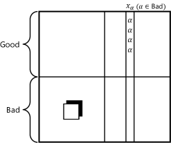
Figure 5: Illustration of ❐, which exclude the $x_{\alpha}$^th column for every $\alpha\in\mathsf{Bad}$.

We show that most of the points of ❐ are colored in $\mathsf{Bad}^{\mathrm{few}}$.

Claim 5.19.

It holds that

$$\Bigl{|}f^{-1}(\mathsf{Bad}^{\mathrm{few}})\cap\text{{\Large\char 112}}\Bigr{|}>0.91\cdot\varepsilon k^{2},$$ (5.72)

namely, more than $0.91\cdot\varepsilon k^{2}$ points of ❐ are colored in $\mathsf{Bad}^{\mathrm{few}}$.

Proof.

The number of points of ❐ not colored in $\mathsf{Bad}^{\mathrm{few}}$ can be bounded as follows:

• Since ❐ does not include $\alpha$^th row for any $\alpha\in\mathsf{Good}$, the number of points colored in $\mathsf{Good}$ is $N_{\mathsf{Good}}<0.01\cdot\varepsilon k^{2}$.

• The number of points colored in $\mathsf{Bad}^{\mathrm{lot}}$ that disagree with $f^{*}$ is $N(\mathsf{Bad}^{\mathrm{lot}})<0.02\cdot\varepsilon k^{2}$.

• The number of points colored in $\mathsf{Bad}^{\mathrm{lot}}$ that agree with $f^{*}$ is

  $$\sum_{\alpha\in\mathsf{Bad}^{\mathrm{lot}}}(k-|D_{\alpha}|)\underbrace{<}_{|D_{\alpha}|>0.99k}0.01k\cdot|\mathsf{Bad}^{\mathrm{lot}}|\underbrace{<}_{|\mathsf{Bad}^{\mathrm{lot}}|<0.01\varepsilon k}10^{-4}\cdot\varepsilon k^{2}.$$ (5.73)

Consequently, the number of points of ❐ colored in $\mathsf{Bad}^{\mathrm{few}}$ is

$$\begin{aligned} \Bigl{|}f^{-1}(\mathsf{Bad}^{\mathrm{few}})\cap\text{{\Large\char 112}}\Bigr{|}&=|\text{{\Large\char 112}}|-\left(N_{\mathsf{Good}}+N(\mathsf{Bad}^{\mathrm{lot}})+\sum_{\alpha\in\mathsf{Bad}^{\mathrm{lot}}}(k-|D_{\alpha}|)\right)\\ &>0.95\cdot\varepsilon k^{2}-\Bigl{(}0.01\cdot\varepsilon k^{2}+0.02\cdot\varepsilon k^{2}+10^{-4}\cdot\varepsilon k^{2}\Bigr{)}>0.91\cdot\varepsilon k^{2},\end{aligned}$$ (5.74)

as desired. ∎

We further partition $\mathsf{Bad}^{\mathrm{few}}$ into $\mathsf{Bad}^{\mathrm{few}}_{\mathrm{long}}$ and $\mathsf{Bad}^{\mathrm{few}}_{\mathrm{short}}$ defined as

$$\begin{aligned} \mathsf{Bad}^{\mathrm{few}}_{\mathrm{long}}&\coloneq\Bigl{\{}\alpha\in\mathsf{Bad}^{\mathrm{few}}\Bigm{|}C_{x_{\alpha},\alpha}\geqslant 0.01k\Bigr{\}},\\ \mathsf{Bad}^{\mathrm{few}}_{\mathrm{short}}&\coloneq\Bigl{\{}\alpha\in\mathsf{Bad}^{\mathrm{few}}\Bigm{|}C_{x_{\alpha},\alpha}<0.01k\Bigr{\}}.\end{aligned}$$ (5.75)

Below, we will divide into two cases according to the size of $\mathsf{Bad}^{\mathrm{few}}_{\mathrm{long}}$.

(Case 2-2-2-1) $|\mathsf{Bad}^{\mathrm{few}}_{\mathrm{long}}|\geqslant 0.2\cdot|\mathsf{Bad}^{\mathrm{few}}|$.

Note that $\mathsf{Bad}^{\mathrm{few}}_{\mathrm{short}}\leqslant 0.8\cdot|\mathsf{Bad}^{\mathrm{few}}|$ by assumption. We first show that a certain fraction of points of ❐ are colored in $\mathsf{Bad}^{\mathrm{few}}_{\mathrm{long}}$.

Claim 5.20.

It holds that

$$\Bigl{|}f^{-1}(\mathsf{Bad}^{\mathrm{few}}_{\mathrm{long}})\cap\text{{\Large\char 112}}\Bigr{|}>0.07\cdot\varepsilon k^{2},$$ (5.76)

namely, more than $0.07\cdot\varepsilon k^{2}$ points of ❐ are colored in $\mathsf{Bad}^{\mathrm{few}}_{\mathrm{long}}$.

Proof.

The number of points colored in $\mathsf{Bad}^{\mathrm{few}}_{\mathrm{short}}$ can be bounded as follows:

• The number of points colored in $\mathsf{Bad}^{\mathrm{few}}_{\mathrm{short}}$ that disagree with $f^{*}$ is

  $$\begin{aligned} N(\mathsf{Bad}^{\mathrm{few}}_{\mathrm{short}})&=\sum_{\alpha\in\mathsf{Bad}^{\mathrm{few}}_{\mathrm{short}}}N_{\alpha}\\ &\underbrace{<}_{N_{\alpha}<1.01k}1.01k\cdot|\mathsf{Bad}^{\mathrm{few}}_{\mathrm{short}}|\\ &\underbrace{\leqslant}_{|\mathsf{Bad}^{\mathrm{few}}_{\mathrm{short}}|\leqslant 0.8\cdot|\mathsf{Bad}|}1.01k\cdot 0.8\cdot|\mathsf{Bad}|\\ &\underbrace{<}_{|\mathsf{Bad}|<1.02\varepsilon k}1.01k\cdot 0.8\cdot 1.02\varepsilon k<0.83\varepsilon k^{2}.\end{aligned}$$ (5.77)

• The number of points colored in $\mathsf{Bad}^{\mathrm{few}}_{\mathrm{short}}$ that agree with $f^{*}$ is

  $$\sum_{\alpha\in\mathsf{Bad}^{\mathrm{few}}_{\mathrm{short}}}(k-|D_{\alpha}|)\underbrace{<}_{|D_{\alpha}|>0.99k}0.01k\cdot|\mathsf{Bad}^{\mathrm{few}}_{\mathrm{short}}|\underbrace{<}_{|\mathsf{Bad}|<1.02\varepsilon k}0.01k\cdot 0.8\cdot 1.02\varepsilon k<0.01\cdot\varepsilon k^{2}.$$ (5.78)

Consequently, by Claim 5.19, the number of points of ❐ colored in $\mathsf{Bad}^{\mathrm{few}}_{\mathrm{long}}$ is

$$\begin{aligned} \Bigl{|}f^{-1}(\mathsf{Bad}^{\mathrm{few}}_{\mathrm{long}})\cap\text{{\Large\char 112}}\Bigr{|}&=\Bigl{|}f^{-1}(\mathsf{Bad}^{\mathrm{few}})\cap\text{{\Large\char 112}}\Bigr{|}-\left(N(\mathsf{Bad}^{\mathrm{few}}_{\mathrm{short}})+\sum_{\alpha\in\mathsf{Bad}^{\mathrm{few}}_{\mathrm{short}}}(k-|D_{\alpha}|)\right)\\ &>0.91\cdot\varepsilon k^{2}-(0.83\cdot\varepsilon k^{2}+0.01\cdot\varepsilon k^{2})=0.07\cdot\varepsilon k^{2},\end{aligned}$$ (5.79)

as desired. ∎

We show that $\mathcal{V}_{\mathrm{stripe}}$’s rejection probability is $\Omega\left(\frac{|f^{-1}(\mathsf{Bad}^{\mathrm{few}}_{\mathrm{long}})\cap\text{{\Large\char 112}}|}{k^{3}}\right)$. See Figure 6 for illustration of its proof.

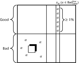
Figure 6: Illustration of the proof of Claim 5.21. Since each color $\alpha$ of $\mathsf{Bad}^{\mathrm{few}}_{\mathrm{long}}$ appears at least $0.01k$ times on the $x_{\alpha}$^th column and $\mathsf{Bad}^{\mathrm{few}}_{\mathrm{long}}$ appears $\Omega(\varepsilon k^{2})$ times in ❐ due to Claim 5.20, we can bound the rejection probability from below.

Claim 5.21.

It holds that

$$\operatorname*{\mathbb{P}}\Bigl{[}\mathcal{V}_{\mathrm{stripe}}\text{ rejects }f\Bigr{]}\geqslant\frac{10^{-3}}{k^{3}}\cdot\Bigl{|}f^{-1}(\mathsf{Bad}^{\mathrm{few}}_{\mathrm{long}})\cap\text{{\Large\char 112}}\Bigr{|}\geqslant\frac{10^{-5}\cdot\varepsilon}{k}.$$ (5.80)

Proof.

For each color $\alpha\in\mathsf{Bad}^{\mathrm{few}}_{\mathrm{long}}$, $\mathcal{V}_{\mathrm{stripe}}$ rejects $f$ by $\alpha$ with probability

$$\begin{aligned} &\operatorname*{\mathbb{P}}\Bigl{[}f(X_{1},Y_{1})=f(X_{2},Y_{2})=\alpha\Bigm{|}X_{1}\neq X_{2}\text{ and }Y_{1}\neq Y_{2}\Bigr{]}\\ &\geqslant\operatorname*{\mathbb{P}}_{\begin{subarray}{c}X_{1}\neq X_{2}\\ Y_{1}\neq Y_{2}\end{subarray}}\Bigl{[}f(X_{1},Y_{1})=f(X_{2},Y_{2})=\alpha\text{ and }X_{1}=x_{\alpha}\text{ and }(X_{2},Y_{2})\in f^{-1}(\alpha)\cap\text{{\Large\char 112}}\Bigr{]}\\ &=\underbrace{\operatorname*{\mathbb{P}}_{\begin{subarray}{c}X_{1}\neq X_{2}\\ Y_{1}\neq Y_{2}\end{subarray}}\Bigl{[}f(X_{1},Y_{1})=f(X_{2},Y_{2})=\alpha\Bigm{|}X_{1}=x_{\alpha}\text{ and }(X_{2},Y_{2})\in f^{-1}(\alpha)\cap\text{{\Large\char 112}}\Bigr{]}}_{\text{(first term)}}\\ &\qquad\cdot\underbrace{\operatorname*{\mathbb{P}}_{\begin{subarray}{c}X_{1}\neq X_{2}\\ Y_{1}\neq Y_{2}\end{subarray}}\Bigl{[}X_{1}=x_{\alpha}\text{ and }(X_{2},Y_{2})\in f^{-1}(\alpha)\cap\text{{\Large\char 112}}\Bigr{]}}_{\text{(second term)}}.\end{aligned}$$ (5.81)

Since $C_{x_{\alpha},\alpha}\geqslant 0.01k$ by definition of $\mathsf{Bad}^{\mathrm{few}}_{\mathrm{long}}$ (i.e., there are $0.01k$ $y$’s such that $f(x_{\alpha},y)=\alpha$) and ❐ does not contain $x_{\alpha}$^th column, the first term can be bounded as follows:

$$\begin{aligned} &\operatorname*{\mathbb{P}}_{\begin{subarray}{c}X_{1}\neq X_{2}\\ Y_{1}\neq Y_{2}\end{subarray}}\Bigl{[}f(X_{1},Y_{1})=f(X_{2},Y_{2})=\alpha\Bigm{|}X_{1}=x_{\alpha}\text{ and }(X_{2},Y_{2})\in f^{-1}(\alpha)\cap\text{{\Large\char 112}}\Bigr{]}\\ &=\operatorname*{\mathbb{P}}_{\begin{subarray}{c}X_{2}\neq x_{\alpha}\\ Y_{1}\neq Y_{2}\end{subarray}}\Bigl{[}f(x_{\alpha},Y_{1})=\alpha\Bigm{|}(X_{2},Y_{2})\in f^{-1}(\alpha)\cap\text{{\Large\char 112}}\Bigr{]}\\ &\geqslant\frac{0.01k-1}{k-1}\underbrace{>}_{k\geqslant k_{0}}10^{-3}.\end{aligned}$$ (5.82)

The second term can be bounded as follows:

$$\begin{aligned} &\operatorname*{\mathbb{P}}_{\begin{subarray}{c}X_{1}\neq X_{2}\\ Y_{1}\neq Y_{2}\end{subarray}}\Bigl{[}X_{1}=x_{\alpha}\text{ and }(X_{2},Y_{2})\in f^{-1}(\alpha)\cap\text{{\Large\char 112}}\Bigr{]}\\ &=\operatorname*{\mathbb{P}}_{\begin{subarray}{c}X_{1}\neq X_{2}\\ Y_{1}\neq Y_{2}\end{subarray}}\Bigl{[}X_{1}=x_{\alpha}\Bigm{|}(X_{2},Y_{2})\in f^{-1}(\alpha)\cap\text{{\Large\char 112}}\Bigr{]}\cdot\operatorname*{\mathbb{P}}_{\begin{subarray}{c}X_{1}\neq X_{2}\\ Y_{1}\neq Y_{2}\end{subarray}}\Bigl{[}(X_{2},Y_{2})\in f^{-1}(\alpha)\cap\text{{\Large\char 112}}\Bigr{]}\\ &\geqslant\frac{1}{k-1}\cdot\frac{|f^{-1}(\alpha)\cap\text{{\Large\char 112}}|}{k^{2}}\geqslant\frac{|f^{-1}(\alpha)\cap\text{{\Large\char 112}}|}{k^{3}}.\end{aligned}$$ (5.83)

Therefore, $\mathcal{V}_{\mathrm{stripe}}$’s rejection probability is at least

$$\begin{aligned} \sum_{\alpha\in\mathsf{Bad}^{\mathrm{few}}_{\mathrm{long}}}\operatorname*{\mathbb{P}}\Bigl{[}\mathcal{V}_{\mathrm{stripe}}\text{ rejects }f\text{ by }\alpha\Bigr{]}&\geqslant\sum_{\alpha\in\mathsf{Bad}^{\mathrm{few}}_{\mathrm{long}}}\frac{10^{-3}}{k^{3}}\cdot\Bigl{|}f^{-1}(\alpha)\cap\text{{\Large\char 112}}\Bigr{|}\\ &=\frac{10^{-3}}{k^{3}}\cdot\Bigl{|}f^{-1}(\mathsf{Bad}^{\mathrm{few}}_{\mathrm{long}})\cap\text{{\Large\char 112}}\Bigr{|}\\ &\underbrace{>}_{\text{\lx@cref{creftype~refnum}{clm:Cut-hard:stripe:far:2221-aux}}}\frac{10^{-3}}{k^{3}}\cdot 0.07\cdot\varepsilon k^{2}>\frac{10^{-5}\cdot\varepsilon}{k},\end{aligned}$$ (5.84)

which completes the proof. ∎

(Case 2-2-2-2) $|\mathsf{Bad}^{\mathrm{few}}_{\mathrm{long}}|<0.2\cdot|\mathsf{Bad}^{\mathrm{few}}|$.

We first show that a large majority of the points of ❐ are colored in $\mathsf{Bad}^{\mathrm{few}}_{\mathrm{short}}$.

Claim 5.22.

The number of points of ❐ colored in $\mathsf{Bad}^{\mathrm{few}}_{\mathrm{short}}$ that disagree with $f^{*}$ is more than $0.68\cdot\varepsilon k^{2}$.

Proof.

Observe the following:

• The number of points colored in $\mathsf{Bad}^{\mathrm{few}}_{\mathrm{long}}$ that disagree with $f^{*}$ is

  $$N(\mathsf{Bad}^{\mathrm{few}}_{\mathrm{long}})\underbrace{<}_{N_{\alpha}<1.01k}1.01k\cdot|\mathsf{Bad}^{\mathrm{few}}_{\mathrm{long}}|\underbrace{<}_{|\mathsf{Bad}^{\mathrm{few}}_{\mathrm{long}}|<0.2|\mathsf{Bad}^{\mathrm{few}}|}1.01k\cdot 0.2\cdot 1.02\varepsilon k<0.21\cdot\varepsilon k^{2}.$$ (5.85)

• The number of points colored in $\mathsf{Bad}^{\mathrm{few}}$ that agree with $f^{*}$ is

  $$\sum_{\alpha\in\mathsf{Bad}^{\mathrm{few}}}(k-|D_{\alpha}|)\underbrace{<}_{|D_{\alpha}|>0.99k}0.01k\cdot|\mathsf{Bad}^{\mathrm{few}}|\underbrace{<}_{|\mathsf{Bad}^{\mathrm{few}}|\leqslant|\mathsf{Bad}|}0.01k\cdot 1.02\varepsilon k<0.02\varepsilon k^{2}.$$ (5.86)

Therefore, by Claim 5.19, the number of points of ❐ colored in $\mathsf{Bad}^{\mathrm{few}}_{\mathrm{short}}$ that disagree with $f^{*}$ is

$$\begin{aligned} &\Bigl{|}f^{-1}(\mathsf{Bad}^{\mathrm{few}})\cap\text{{\Large\char 112}}\Bigr{|}-\left(N(\mathsf{Bad}^{\mathrm{few}}_{\mathrm{long}})+\sum_{\alpha\in\mathsf{Bad}^{\mathrm{few}}}(k-|D_{\alpha}|)\right)\\ &>0.91\cdot\varepsilon k^{2}-(0.21\cdot\varepsilon k^{2}+0.02\cdot\varepsilon k^{2})>0.68\cdot\varepsilon k^{2},\end{aligned}$$ (5.87)

as desired. ∎

Claim 5.22 implies $N(\mathsf{Bad}^{\mathrm{few}}_{\mathrm{short}})>0.68\cdot\varepsilon k^{2}$. Define

$$\widetilde{\mathsf{Bad}^{\mathrm{few}}_{\mathrm{short}}}\coloneq\Bigl{\{}\alpha\in\mathsf{Bad}^{\mathrm{few}}_{\mathrm{short}}\Bigm{|}N_{\alpha}\geqslant 0.01k\Bigr{\}}.$$ (5.88)

Observe that

$$\begin{aligned} N\Bigl{(}\widetilde{\mathsf{Bad}^{\mathrm{few}}_{\mathrm{short}}}\Bigr{)}&\geqslant N(\mathsf{Bad}^{\mathrm{few}}_{\mathrm{short}})-\sum_{\alpha\in\mathsf{Bad}^{\mathrm{few}}_{\mathrm{short}}}N_{\alpha}\cdot\Bigl{\llbracket}N_{\alpha}<0.01k\Bigr{\rrbracket}\\ &\geqslant N(\mathsf{Bad}^{\mathrm{few}}_{\mathrm{short}})-0.01k\cdot|\mathsf{Bad}^{\mathrm{few}}_{\mathrm{short}}|\\ &\geqslant N(\mathsf{Bad}^{\mathrm{few}}_{\mathrm{short}})-0.01k\cdot|\mathsf{Bad}|\\ &\geqslant 0.68\varepsilon k^{2}-0.01k\cdot 1.02\varepsilon k\\ &>0.66\varepsilon k^{2}.\end{aligned}$$ (5.89)

We will show that $\mathcal{V}_{\mathrm{stripe}}$’s rejection probability is $\Omega\left(\frac{1}{k^{3}}\cdot N\Bigl{(}\widetilde{\mathsf{Bad}^{\mathrm{few}}_{\mathrm{short}}}\Bigr{)}\right)$. See Figure 7 for illustration of its proof.

Figure 7: Illustration of the proof of Claim 5.23. Since $\alpha\in\widetilde{\mathsf{Bad}^{\mathrm{few}}_{\mathrm{short}}}$ appears at most $0.55k$ times for any column and row and $N\Bigl{(}\widetilde{\mathsf{Bad}^{\mathrm{few}}_{\mathrm{short}}}\Bigr{)}=\Omega(\varepsilon k^{2})$ due to Claim 5.22, we can apply Lemma 5.15 to bound the rejection probability from below.

Claim 5.23.

$$\operatorname*{\mathbb{P}}\Bigl{[}\mathcal{V}_{\mathrm{stripe}}\text{ rejects }f\Bigr{]}\geqslant\frac{10^{-5}}{k^{3}}\cdot\left(N\Bigl{(}\widetilde{\mathsf{Bad}^{\mathrm{few}}_{\mathrm{short}}}\Bigr{)}-0.6k\cdot\Bigl{|}\widetilde{\mathsf{Bad}^{\mathrm{few}}_{\mathrm{short}}}\Bigr{|}\right)\geqslant\frac{10^{-6}\cdot\varepsilon}{k}.$$ (5.90)

Proof.

For each color $\alpha\in\widetilde{\mathsf{Bad}^{\mathrm{few}}_{\mathrm{short}}}$, we claim that $R_{y,\alpha}<0.55k$ for all $y\in[k]$. Suppose for contradiction that $R_{y^{*},\alpha}\geqslant 0.55k$ for some $y^{*}\in[k]$. Note that $y^{*}\neq\alpha$ as $R_{\alpha,\alpha}=k-|D_{\alpha}|<0.01k$ by definition of $\mathsf{Bad}$. Since $f^{*}$ is closest to $f$, we must have

$$\begin{aligned} &R_{\alpha,\alpha}+R_{y^{*},y^{*}}\geqslant R_{\alpha,y^{*}}+R_{y^{*},\alpha}\\ &\implies R_{y^{*},y^{*}}\geqslant R_{\alpha,y^{*}}+R_{y^{*},\alpha}-R_{\alpha,\alpha}\geqslant R_{y^{*},\alpha}-R_{\alpha,\alpha}>0.54k\\ &\implies R_{y^{*},\alpha}+R_{y^{*},y^{*}}>k,\end{aligned}$$ (5.91)

which is a contradiction.

Since $C_{x,\alpha}<0.01k<0.55k$ for all $x\in[k]$ by definition of $\mathsf{Bad}^{\mathrm{few}}_{\mathrm{short}}$, we apply Lemma 5.15 with $\vartheta=0.55$ to every color $\alpha\in\widetilde{\mathsf{Bad}^{\mathrm{few}}_{\mathrm{short}}}$ and derive

$$\operatorname*{\mathbb{P}}\Bigl{[}\mathcal{V}_{\mathrm{stripe}}\text{ rejects }f\text{ by }\alpha\Bigr{]}\geqslant\frac{N_{\alpha}\cdot(N_{\alpha}-0.55k)}{10^{2}\cdot k^{3}}\geqslant\frac{0.01k\cdot(N_{\alpha}-0.55k)}{10^{2}\cdot k^{3}}=\frac{N_{\alpha}-0.55k}{10^{4}\cdot k^{3}}.$$ (5.92)

Therefore, $\mathcal{V}_{\mathrm{stripe}}$’s rejection probability is at least

$$\begin{aligned} \operatorname*{\mathbb{P}}\Bigl{[}\mathcal{V}_{\mathrm{stripe}}\text{ rejects }f\Bigr{]}&\geqslant\sum_{\alpha\in\widetilde{\mathsf{Bad}^{\mathrm{few}}_{\mathrm{short}}}}\frac{N_{\alpha}-0.55k}{10^{4}\cdot k^{3}}\\ &\geqslant\frac{10^{-4}}{k^{3}}\cdot\left(N\Bigl{(}\widetilde{\mathsf{Bad}^{\mathrm{few}}_{\mathrm{short}}}\Bigr{)}-0.55k\cdot\Bigl{|}\widetilde{\mathsf{Bad}^{\mathrm{few}}_{\mathrm{short}}}\Bigr{|}\right)\\ &\geqslant\frac{10^{-4}}{k^{3}}\cdot\left(N\Bigl{(}\widetilde{\mathsf{Bad}^{\mathrm{few}}_{\mathrm{short}}}\Bigr{)}-0.55k\cdot|\mathsf{Bad}|\right)\\ &\geqslant\frac{10^{-4}}{k^{3}}\cdot\Bigl{(}0.66\cdot\varepsilon k^{2}-0.55k\cdot 1.02\varepsilon k\Bigr{)}>\frac{10^{-6}\cdot\varepsilon}{k},\end{aligned}$$ (5.93)

which completes the proof. ∎

Using the claims shown so far, we eventually prove Lemma 5.7.

Proof of Lemma 5.7.

By Claims 5.16, 5.17, 5.18, 5.21 and 5.23, the following hold:

• If $f$ is $\varepsilon$-far from being striped for any $\varepsilon<\varepsilon_{0}=10^{-2}$, then $\mathcal{V}_{\mathrm{stripe}}$ rejects with probability more than $\frac{10^{-6}\cdot\varepsilon}{k}$.

• If $f$ is $10^{-2}$-far from being striped, then $\mathcal{V}_{\mathrm{stripe}}$ rejects with probability more than $\frac{10^{-6}\cdot 10^{-2}}{k}$.

Setting the rejection rate $\rho\coloneq 10^{-8}$ completes the proof. ∎

6 Approximation Algorithm of Maxmin $k$-Cut Reconfiguration

The result of this section is a deterministic $\left(1-\frac{2}{k}\right)$-factor approximation algorithm for Maxmin $k$-Cut Reconfiguration for all $k\geqslant 2$.

Theorem 6.1.

For every integer $k\geqslant 2$ and every number $\varepsilon>0$, there exists a deterministic polynomial-time algorithm that given a simple graph $G$ and its two $k$-colorings $f_{\mathsf{start}},f_{\mathsf{end}}$, returns a reconfiguration sequence $\mathscr{F}$ from $f_{\mathsf{start}}$ to $f_{\mathsf{end}}$ such that

$$\operatorname{\mathsf{val}}_{G}(\mathscr{F})\geqslant\left(1-\frac{1}{k}-\varepsilon\right)^{2}\cdot\min\Big{\{}\operatorname{\mathsf{val}}_{G}(f_{\mathsf{start}}),\operatorname{\mathsf{val}}_{G}(f_{\mathsf{end}})\Bigr{\}}.$$ (6.1)

In particular, letting $\varepsilon\coloneq\frac{1}{k^{3}}$, this algorithm approximates Maxmin $k$-Cut Reconfiguration on simple graphs within a factor of $\left(1-\frac{1}{k}-\frac{1}{k^{3}}\right)^{2}\geqslant 1-\frac{2}{k}$.

6.1 Outline of the Proof of Theorem 6.1

Our proof of Theorem 6.1 can be divided into the following three steps:

• In Section 6.2, we deal with the case that $f_{\mathsf{start}}$ or $f_{\mathsf{end}}$ has a low value, say $o(1)$. We show how to safely transform such a $k$-coloring into a $\frac{1}{2}$-value $k$-coloring.

• In Section 6.3, for a graph of bounded degree, we demonstrate that a random reconfiguration sequence via a random $k$-coloring makes $\approx\left(1-\frac{1}{k}\right)^{2}$-fraction of edges bichromatic with high probability, which is based on the read-$k$ Chernoff bound (Theorem 4.7).

• In Section 6.4, we handle high-degree vertices. Intuitively, $k$ colors are distributed almost evenly over each high-degree vertex’s neighbors with high probability.

6.2 Low-value Case

Here, we introduce the following lemma, which enables us to assume that $\operatorname{\mathsf{val}}_{G}(f_{\mathsf{start}})$ and $\operatorname{\mathsf{val}}_{G}(f_{\mathsf{end}})$ are at least $\frac{1}{2}$ without loss of generality.

Lemma 6.2.

For a graph $G=(V,E)$ and its $k$-coloring $f_{\mathsf{start}}\colon V\to[k]$ such that $\operatorname{\mathsf{val}}_{G}(f_{\mathsf{start}})<1-\frac{1}{k}$, there exists a reconfiguration sequence $\mathscr{F}$ from $f_{\mathsf{start}}$ to another $k$-coloring $f^{\prime}\colon V\to[k]$ such that $\operatorname{\mathsf{val}}_{G}(f^{\prime})\geqslant 1-\frac{1}{k}$ and $\operatorname{\mathsf{val}}_{G}(\mathscr{F})=\operatorname{\mathsf{val}}_{G}(f_{\mathsf{start}})$. Such $\mathscr{F}$ can be found in polynomial time.

Proof.

We first claim the following:

Claim 6.3.

For a $k$-coloring $f\colon V\to[k]$ with $\operatorname{\mathsf{val}}_{G}(f)<1-\frac{1}{k}$, there is another $k$-coloring $f^{\prime}\colon V\to[k]$ such that $\operatorname{\mathsf{val}}_{G}(f^{\prime})>\operatorname{\mathsf{val}}_{G}(f)$ and $f$ and $f^{\prime}$ differ in a single vertex.

Proof.

We prove the contrapositive. Suppose that recoloring any single vertex does not decrease the number of monochromatic edges. Then, for every $v\in V$, $f(v)$ appears in at most $\frac{1}{k}$-fraction of $v$’s neighbors; i.e., at least $\left(1-\frac{1}{k}\right)$-fraction of the incident edges to $v$ must be bichromatic. This implies $\operatorname{\mathsf{val}}_{G}(f)\geqslant 1-\frac{1}{k}$. ∎

By the above claim, until $\operatorname{\mathsf{val}}_{G}(f)\geqslant 1-\frac{1}{k}$, one can find a pair of vertex $v\in V$ and color $\alpha\in[k]$ such that recoloring $v$ to $\alpha$ strictly increases the number of bichromatic edges, as desired. ∎

6.3 Low-degree Case

We then prove that if $G$ has bounded degree, any proper $k$-coloring of $G$ can be safely transformed into a random $k$-coloring with high probability.

Lemma 6.4.

Let $G=(V,E)$ be a graph of maximum degree at most $\Delta\coloneq|E|^{\frac{2}{3}}$ and $f_{\mathsf{start}}\colon V\to[k]$ be its proper $k$-coloring. Consider a uniformly random $k$-coloring $F\colon V\to[k]$ and a random irredundant reconfiguration sequence $\mathscr{F}$ uniformly chosen from $\mathbb{F}(f_{\mathsf{start}}\leftrightsquigarrow F)$. Then, it holds that

$$\operatorname*{\mathbb{P}}_{\mathscr{F}}\left[\operatorname{\mathsf{val}}_{G}(\mathscr{F})<\left(1-\tfrac{1}{k}\right)^{2}-m^{-\frac{1}{4}}\right]<\exp\left(-2\cdot m^{\frac{1}{12}}\right).$$ (6.2)

To prove Lemma 6.4, we first show that each edge consistently remains bichromatic through $\mathscr{F}$ with probability $\left(1-\frac{1}{k}\right)^{2}$.

Lemma 6.5.

Let $e=(v,w)$ be an edge and $f_{\mathsf{start}}\colon\{v,w\}\to[k]$ be its proper $k$-coloring. Consider a uniformly random $k$-coloring $F\colon\{v,w\}\to[k]$ and a random irredundant reconfiguration sequence $\mathscr{F}$ uniformly chosen from $\mathbb{F}(f_{\mathsf{start}}\leftrightsquigarrow F)$. Then, $\mathscr{F}$ keeps $e$ bichromatic with probability at least $\left(1-\frac{1}{k}\right)^{2}$; namely,

$$\operatorname*{\mathbb{P}}\Bigl{[}\forall f\in\mathscr{F},\;f(v)\neq f(w)\Bigr{]}\geqslant\left(1-\tfrac{1}{k}\right)^{2}.$$ (6.3)

Proof.

Denote $\alpha_{v}\coloneq F(v)$, $\alpha_{w}\coloneq F(w)$, and $f_{\mathsf{start}}(e)\coloneq\{f_{\mathsf{start}}(v),f_{\mathsf{start}}(w)\}$. Consider the following case analysis on $\alpha_{v}$ and $\alpha_{w}$:

• (Case 1) If $\alpha_{v}\neq\alpha_{w}$ and $\{\alpha_{v},\alpha_{w}\}\cap\{f_{\mathsf{start}}(v),f_{\mathsf{start}}(w)\}=\emptyset$: There are $(k-2)(k-3)$ such colorings in total. Observe easily that $\mathscr{F}$ succeeds with probability $1$.

• (Case 2) If $\alpha_{v}=f_{\mathsf{start}}(v)$ and $\alpha_{w}\notin f_{\mathsf{start}}(e)$: There are $(k-2)$ such colorings. $\mathscr{F}$ succeeds with probability $1$.

• (Case 3) If $\alpha_{w}=f_{\mathsf{start}}(w)$ and $\alpha_{v}\notin f_{\mathsf{start}}(e)$: There are $(k-2)$ such colorings. Similarly to (Case 3), $\mathscr{F}$ succeeds with probability $1$.

• (Case 4) If $\alpha_{v}=f_{\mathsf{start}}(v)$ and $\alpha_{w}=f_{\mathsf{start}}(w)$: There is only one such coloring; $\mathscr{F}$ always succeeds.

• (Case 5) If $\alpha_{v}=f_{\mathsf{start}}(w)$ and $\alpha_{w}\notin f_{\mathsf{start}}(e)$: There are $(k-2)$ such colorings. If $w$ is recolored at first, $\mathscr{F}$ fails; i.e., the success probability is $\frac{1}{2}$.

• (Case 6) If $\alpha_{w}=f_{\mathsf{start}}(v)$ and $\alpha_{v}\notin f_{\mathsf{start}}(e)$: There are $(k-2)$ such colorings. Similarly to the previous case, $\mathscr{F}$ succeeds with probability $\frac{1}{2}$.

• (Case 7) If $\alpha_{v}=f_{\mathsf{start}}(w)$ and $\alpha_{w}=f_{\mathsf{start}}(v)$: There is only one such coloring. $\mathscr{F}$ cannot succeed anyway.

• (Case 8) Otherwise (i.e., $\alpha_{v}=\alpha_{w}$): There are $k$ such colorings; $\mathscr{F}$ never succeeds.

Summing the success probability over the preceding eight cases, we derive

$$\begin{aligned} &k^{-2}\cdot\Bigl{(}(k-2)(k-3)\cdot 1+(k-2)\cdot 1+(k-2)\cdot 1+1\cdot 1+(k-2)\cdot\tfrac{1}{2}+(k-2)\cdot\tfrac{1}{2}\Bigr{)}\\ &=\left(1-\frac{1}{k}\right)^{2}\end{aligned}$$ (6.4)

completing the proof. ∎

We now apply the read-$k$ Chernoff inequality to Lemma 6.5 and prove Lemma 6.4.

Proof of Lemma 6.4.

Define $n\coloneq|V|$ and $m\coloneq|E|$. Let $\mathbf{I}=(I_{v})_{v\in V}$ be a random integer sequence distributed uniformly over $[k]^{V}$ and $f_{\mathbf{I}}\colon V\to[k]$ denote a $k$-coloring of $G$ such that $f_{\mathbf{I}}(v)\coloneq I_{v}$ for all $v\in V$. Let $\mathbf{R}=(R_{v})_{v\in V}$ be a random real sequence distributed uniformly over $(0,1)^{V}$ and $\sigma_{\mathbf{R}}\colon[n]\to V$ denote an ordering of $V$ such that $R_{\sigma(1)}>R_{\sigma(2)}>\cdots>R_{\sigma(n)}$. Let $\mathscr{F}(\mathbf{I},\mathbf{R};f_{\mathsf{start}})$ be a random irredundant reconfiguration sequence from $f_{\mathsf{start}}$ to $f_{\mathbf{I}}$ obtained by recoloring vertex $\sigma(i)$ from $f_{\mathsf{start}}(\sigma(i))$ to $f_{\mathbf{I}}(\sigma(i))$ (if $f_{\mathsf{start}}(\sigma(i))\neq f_{\mathbf{I}}(\sigma(i))$) in the order of $\sigma(1),\ldots,\sigma(n)$. Observe easily that $\mathscr{F}(\mathbf{I},\mathbf{R};f_{\mathsf{start}})$ is uniformly distributed over $\mathbb{F}(f_{\mathsf{start}}\leftrightsquigarrow F)$.

For each edge $e=(v,w)$ of $G$, let $Y_{e}$ be a random variable that takes $1$ if $e$ is bichromatic throughout $\mathscr{F}(\mathbf{I},\mathbf{R};f_{\mathsf{start}})$ and takes $0$ otherwise; namely,

$$Y_{e}\coloneq\Bigl{\llbracket}\forall f\in\mathscr{F}(\mathbf{I},\mathbf{R};f_{\mathsf{start}}),\;f(v)\neq f(w)\Bigr{\rrbracket}.$$ (6.5)

Note that each $Y_{e}$ is Boolean and depends only on $\mathbf{I}|_{e}$ and $\mathbf{R}|_{e}$; $Y_{e}$’s thus are a read-$\Delta$ family. Let $Y$ be the sum of $Y_{e}$ over all edges $e$; namely,

$$Y\coloneq\sum_{e\in E}Y_{e}.$$ (6.6)

Since $\mathscr{F}(\mathbf{I},\mathbf{R};f_{\mathsf{start}})$ is distributed uniformly over $\mathbb{F}(f_{\mathsf{start}}\leftrightsquigarrow F)$, by Lemma 6.5, it holds that

$$\operatorname*{\mathbb{E}}[Y]\geqslant\left(1-\tfrac{1}{k}\right)^{2}\cdot m.$$ (6.7)

By applying the read-$k$ Chernoff bound (Theorem 4.7) to $Y_{e}$’s, we derive

$$\operatorname*{\mathbb{P}}\Bigl{[}Y\leqslant\operatorname*{\mathbb{E}}[Y]-m^{\frac{3}{4}}\Bigr{]}\leqslant\exp\left(-\frac{2\cdot m^{\frac{3}{4}}}{\Delta}\right)\underbrace{<}_{\Delta=m^{\frac{2}{3}}}\exp\left(-2\cdot m^{\frac{1}{12}}\right),$$ (6.8)

which completes the proof. ∎

6.4 Handling High-degree Vertices

We now handle high-degree vertices and show the following using Lemma 6.4.

Proposition 6.6.

Let $G=(V,E)$ be a simple graph such that $|E|\geqslant 10^{6}$, and $f_{\mathsf{start}}\colon V\to[k]$ be its $k$-coloring such that $\operatorname{\mathsf{val}}_{G}(f_{\mathsf{start}})\geqslant\frac{1}{2}$. Let $\Delta\coloneq|E|^{\frac{2}{3}}$, and $V_{\leqslant\Delta}$ and $V_{>\Delta}$ be the set of vertices in $G$ whose degree is at most and greater than $\Delta$, respectively.

Consider a uniformly random $k$-coloring $F\colon V\to[k]$ and a random reconfiguration sequence $\mathscr{F}$ from $f_{\mathsf{start}}$ to $F$ uniformly chosen from $\mathbb{F}(f_{\mathsf{start}}\leftrightsquigarrow f^{\circ}\leftrightsquigarrow F)$, where $f^{\circ}$ agrees with $f_{\mathsf{start}}$ on $V_{>\Delta}$ and with $F$ on $V_{\leqslant\Delta}$. Then, it holds that

$$\operatorname*{\mathbb{P}}_{\mathscr{F}}\left[\operatorname{\mathsf{val}}_{G}(\mathscr{F})<\left(1-\tfrac{1}{k}\right)^{2}\cdot\operatorname{\mathsf{val}}_{G}(f_{\mathsf{start}})-5\cdot m^{-\frac{1}{4}}\right]<\exp\left(-\Omega\left(k^{-5}\cdot m^{\frac{1}{24}}\right)\right).$$ (6.9)

Define $n\coloneq|V|$, $m\coloneq|E|$, and

$$\begin{aligned} V_{\leqslant\Delta}\coloneq\Bigl{\{}v\in V\Bigm{|}d_{G}(v)\leqslant\Delta\Bigr{\}},\\ V_{>\Delta}\coloneq\Bigl{\{}v\in V\Bigm{|}d_{G}(v)>\Delta\Bigr{\}}.\end{aligned}$$ (6.10)

Partition $G$ into the following three subgraphs:

$$\begin{aligned} G_{1}&\coloneq G[V_{\leqslant\Delta}],&m_{1}&\coloneq|E(G_{1})|,\\ G_{2}&\coloneq G-(E(G[V_{\leqslant\Delta}])\cup E(G[V_{>\Delta}])),&m_{2}&\coloneq|E(G_{2})|,\\ G_{3}&\coloneq G[V_{>\Delta}],&m_{3}&\coloneq|E(G_{3})|.\end{aligned}$$ (6.11)

Note that the union of $G_{1}$, $G_{2}$, and $G_{3}$ is equal to $G$. Since $|V_{>\Delta}|\cdot\Delta<2m$, it holds that $|V_{>\Delta}|<2\cdot m^{\frac{1}{3}}$; thus, $m_{3}\leqslant|V_{>\Delta}|^{2}<4\cdot m^{\frac{2}{3}}$.

Let $m_{1}^{\prime}$, $m_{2}^{\prime}$, and $m_{3}^{\prime}$ denote the number of bichromatic edges in $G_{1}$, $G_{2}$, and $G_{3}$, with respect to $f_{\mathsf{start}}$, respectively; namely,

$$\begin{aligned} m_{1}^{\prime}&\coloneq m_{1}\cdot\operatorname{\mathsf{val}}_{G_{1}}(f_{\mathsf{start}}),\\ m_{2}^{\prime}&\coloneq m_{2}\cdot\operatorname{\mathsf{val}}_{G_{2}}(f_{\mathsf{start}}),\\ m_{3}^{\prime}&\coloneq m_{3}\cdot\operatorname{\mathsf{val}}_{G_{3}}(f_{\mathsf{start}}).\end{aligned}$$ (6.12)

Note that $m_{1}^{\prime}+m_{2}^{\prime}+m_{3}^{\prime}=m\cdot\operatorname{\mathsf{val}}_{G}(f_{\mathsf{start}})\geqslant\frac{m}{2}$.

We first demonstrate that the number of edges of $G_{2}$ that are bichromatic throughout $\mathscr{F}$, i.e., $m_{2}\cdot\operatorname{\mathsf{val}}_{G_{2}}(\mathscr{F})$, is at least $\left(1-\frac{1}{k}\right)^{2}\cdot m_{2}^{\prime}$ with high probability.

Lemma 6.7.

It holds that

$$\operatorname*{\mathbb{P}}\Bigl{[}m_{2}\cdot\operatorname{\mathsf{val}}_{G_{2}}(\mathscr{F})<\left(1-\tfrac{1}{k}\right)^{2}\cdot m_{2}^{\prime}\Bigr{]}<4\cdot m^{\frac{2}{3}}\cdot\exp\left(-\frac{m_{2}^{\prime}}{48k^{5}\cdot m^{\frac{1}{3}}}\right).$$ (6.13)

Proof.

Fix $v\in V_{>\Delta}$. Let $X_{v}$ denote a random variable for the maximum number of edges between $v$ and $V_{\leqslant\Delta}$ that are monochromatic over all $k$-colorings of $\mathscr{F}$; namely,

$$X_{v}\coloneq\max_{f\in\mathscr{F}}\left\{\sum_{w\in\mathcal{N}_{G}(v)\cap V_{\leqslant\Delta}}\Bigl{\llbracket}f(v)=f(w)\Bigr{\rrbracket}\right\}.$$ (6.14)

Observe easily that

$$m_{2}\cdot\operatorname{\mathsf{val}}_{G_{2}}(\mathscr{F})\geqslant\sum_{v\in V_{>\Delta}}\Bigl{(}|\mathcal{N}_{G}(v)\cap V_{\leqslant\Delta}|-X_{v}\Bigr{)}.$$ (6.15)

Let $M_{v}$ and $B_{v}$ be the set of vertices $w\in\mathcal{N}_{G}(v)\cap V_{\leqslant\Delta}$ such that $(v,w)$ is monochromatic and bichromatic with respect to $f_{\mathsf{start}}$, respectively; namely,

$$M_{v} \coloneq\Bigl{\{}w\in\mathcal{N}_{G}(v)\cap V_{\leqslant\Delta}\Bigm{|}f_{\mathsf{start}}(v)=f_{\mathsf{start}}(w)\Bigr{\}},$$ (6.16)

$$B_{v} \coloneq\Bigl{\{}w\in\mathcal{N}_{G}(v)\cap V_{\leqslant\Delta}\Bigm{|}f_{\mathsf{start}}(v)\neq f_{\mathsf{start}}(w)\Bigr{\}}.$$ (6.17)

Note that $M_{v}$ and $B_{v}$ form a partition of $\mathcal{N}_{G}(v)\cap V_{\leqslant\Delta}$, and

$$\sum_{v\in V_{\leqslant\Delta}}|B_{v}|=m_{2}^{\prime}.$$ (6.18)

Since $f_{\mathsf{start}}$ makes all edges of $B_{v}$ bichromatic, and $v$ would be recolored after vertices of $B_{v}$ are recolored in $\mathscr{F}$, we derive

$$\begin{aligned} X_{v}&\leqslant|M_{v}|+\max\left\{\sum_{w\in B_{v}}\Bigl{\llbracket}f_{\mathsf{start}}(v)=F(w)\Bigr{\rrbracket},\sum_{w\in B_{v}}\Bigl{\llbracket}F(v)=F(w)\Bigr{\rrbracket}\right\}\\ &\leqslant|M_{v}|+\max_{\alpha\in[k]}\left\{\sum_{w\in B_{v}}\Bigl{\llbracket}\alpha=F(w)\Bigr{\rrbracket}\right\}\\ &\leqslant|M_{v}|+\max_{\alpha\in[k]}\left|\Bigl{\{}w\in B_{v}\Bigm{|}F(w)=\alpha\Bigr{\}}\right|\\ &=|M_{v}|+\max_{\alpha\in[k]}\left\{Y_{\alpha}\right\},\end{aligned}$$ (6.19)

where $Y_{1},\ldots,Y_{k}$ are random variables that follow the multinomial distribution with $|B_{v}|$ trials and event probabilities $\underbrace{\tfrac{1}{k},\ldots,\tfrac{1}{k}}_{k\text{ times}}$. Here, the maximum of $Y_{i}$’s may exceed $\left(\frac{1}{k}+\varepsilon\right)n$ with small probability, which will be proved later.

Claim 6.8.

For $k$ random variables, $Y_{1},\ldots,Y_{k}$, that follow the multinomial distribution with $n$ trials and event probabilities $\underbrace{\tfrac{1}{k},\ldots,\tfrac{1}{k}}_{k\text{ times}}$, it holds that for any $\varepsilon>0$,

$$\operatorname*{\mathbb{P}}\left[\max_{1\leqslant i\leqslant k}\{Y_{i}\}>\left(\tfrac{1}{k}+\varepsilon\right)\cdot n\right]<n\cdot\exp\left(-\frac{\varepsilon^{2}kn}{3}\right).$$ (6.20)

By taking a union bound of Claim 6.8 over all $v\in V_{>\Delta}$ such that $|B_{v}|\geqslant\frac{\varepsilon\cdot m_{2}^{\prime}}{|V_{>\Delta}|}$, with probability at least $1-|V_{>\Delta}|^{2}\cdot\exp\left(-\frac{\varepsilon^{2}k}{3}\frac{\varepsilon\cdot m_{2}^{\prime}}{|V_{>\Delta}|}\right)$, it holds that

$$X_{v}\leqslant|M_{v}|+\left(\tfrac{1}{k}+\varepsilon\right)\cdot|B_{v}|\text{ for all }v\in V_{>\Delta}\text{ such that }|B_{v}|\geqslant\frac{\varepsilon\cdot m_{2}^{\prime}}{|V_{>\Delta}|}.$$ (6.21)

In such a case, we derive

$$\begin{aligned} m_{2}\cdot\operatorname{\mathsf{val}}_{G_{2}}(\mathscr{F})&\geqslant\sum_{v\in V_{>\Delta}}\Bigl{(}|\mathcal{N}_{G}(v)\cap V_{\leqslant\Delta}|-X_{v}\Bigr{)}\\ &\geqslant\sum_{v\in V_{>\Delta}:|B_{v}|\geqslant\frac{\varepsilon\cdot m_{2}^{\prime}}{|V_{>\Delta}|}}\Bigl{(}|M_{v}|+|B_{v}|-X_{v}\Bigr{)}\\ &\geqslant\sum_{v\in V_{>\Delta}:|B_{v}|\geqslant\frac{\varepsilon\cdot m_{2}^{\prime}}{|V_{>\Delta}|}}\Bigl{(}|M_{v}|+|B_{v}|-\Bigl{(}|M_{v}|+\left(\tfrac{1}{k}+\varepsilon\right)\cdot|B_{v}|\Bigr{)}\Bigr{)}\\ &=\left(1-\tfrac{1}{k}-\varepsilon\right)\cdot\sum_{v\in V_{>\Delta}:|B_{v}|\geqslant\frac{\varepsilon\cdot m_{2}^{\prime}}{|V_{>\Delta}|}}|B_{v}|\\ &=\left(1-\tfrac{1}{k}-\varepsilon\right)\cdot\left(\sum_{v\in V_{>\Delta}}|B_{v}|-\sum_{v\in V_{>\Delta}:|B_{v}|<\frac{\varepsilon\cdot m_{2}^{\prime}}{|V_{>\Delta}|}}|B_{v}|\right)\\ &\geqslant\left(1-\tfrac{1}{k}-\varepsilon\right)\cdot(1-\varepsilon)\cdot m_{2}^{\prime}.\end{aligned}$$ (6.22)

Setting finally $\varepsilon\coloneq\frac{1}{2k^{2}}$, we have

$$m_{2}\cdot\operatorname{\mathsf{val}}_{G_{2}}(\mathscr{F})\geqslant\left(1-\tfrac{1}{k}-\varepsilon\right)\cdot(1-\varepsilon)\cdot m_{2}^{\prime}\geqslant\left(1-\tfrac{1}{k}\right)^{2}\cdot m_{2}^{\prime}$$ (6.23)

with probability at least

$$1-|V_{>\Delta}|^{2}\cdot\exp\left(-\frac{\varepsilon^{2}k}{3}\frac{\varepsilon\cdot m_{2}^{\prime}}{|V_{>\Delta}|}\right)\geqslant 1-4\cdot m^{\frac{2}{3}}\cdot\exp\left(-\frac{m_{2}^{\prime}}{48k^{5}\cdot m^{\frac{1}{3}}}\right),$$ (6.24)

where we used the fact that $|V_{>\Delta}|<2\cdot m^{\frac{1}{3}}$, as desired. ∎

Proof of Claim 6.8.

It is sufficient to bound $\operatorname*{\mathbb{P}}[Y_{i}>(\frac{1}{k}+\varepsilon)n]$. Since $Y_{i}$ follows a binomial distribution with $n$ trials and event probability $\frac{1}{k}$, which has mean $\operatorname*{\mathbb{E}}[Y_{i}]=\frac{n}{k}$, we apply the Chernoff bound (Theorem 4.5) to obtain

$$\operatorname*{\mathbb{P}}\Bigl{[}Y_{i}\geqslant(1+k\varepsilon)\operatorname*{\mathbb{E}}[Y_{i}]\Bigr{]}\leqslant\exp\left(-\frac{k^{2}\varepsilon^{2}\cdot\operatorname*{\mathbb{E}}[Y_{i}]}{3}\right)=\exp\left(-\frac{\varepsilon^{2}kn}{3}\right).$$ (6.25)

Taking a union bound over $Y_{i}$’s accomplishes the proof. ∎

We are now ready to prove Proposition 6.6.

Proof of Proposition 6.6.

Since $\mathscr{F}$ is uniformly distributed over $\mathbb{F}(f_{\mathsf{start}}\leftrightsquigarrow f^{\circ})$, we apply Lemma 6.4 to the subgraph of $G_{1}$ induced by bichromatic edges with respect to $f_{\mathsf{start}}$ and obtain

$$\begin{aligned} \operatorname*{\mathbb{P}}\left[m_{1}\cdot\operatorname{\mathsf{val}}_{G_{1}}(\mathscr{F})<\left(1-\tfrac{1}{k}\right)^{2}\cdot m_{1}^{\prime}-m_{1}^{\prime\frac{3}{4}}\right]<\exp\left(-2\cdot m_{1}^{\prime\frac{1}{12}}\right).\end{aligned}$$ (6.26)

By Lemma 6.7, we have

$$\operatorname*{\mathbb{P}}\left[m_{2}\cdot\operatorname{\mathsf{val}}_{G_{2}}(\mathscr{F})<\left(1-\tfrac{1}{k}\right)^{2}\cdot m_{2}^{\prime}\right]<4\cdot m^{\frac{2}{3}}\cdot\exp\left(-\frac{m_{2}^{\prime}}{48k^{5}\cdot m^{\frac{1}{3}}}\right).$$ (6.27)

We proceed by a case analysis on $m_{1}^{\prime}$ and $m_{2}^{\prime}$:

• (Case 1) if $m_{1}^{\prime}\leqslant m^{\frac{1}{2}}$: Since $m_{1}^{\prime}+m_{3}^{\prime}\leqslant m^{\frac{1}{2}}+4\cdot m^{\frac{2}{3}}\leqslant 5\cdot m^{\frac{2}{3}}$, we have

  $$\begin{aligned} m_{2}^{\prime}&=(m_{1}^{\prime}+m_{2}^{\prime}+m_{3}^{\prime})-(m_{1}^{\prime}+m_{3}^{\prime})\\ &\geqslant m\cdot\operatorname{\mathsf{val}}_{G}(f)-5\cdot m^{\frac{2}{3}}\\ &\geqslant\tfrac{1}{2}\cdot m-5\cdot m^{\frac{2}{3}}\underbrace{\geqslant}_{m\geqslant 10^{6}}\tfrac{1}{4}\cdot m.\end{aligned}$$ (6.28)

  Therefore, with probability at least

  $$1-\text{\lx@cref{creftype~refnum}{eq:Cut-alg:high-prob:high-degree}}=1-4\cdot m^{\frac{2}{3}}\cdot\exp\left(-\frac{m_{2}^{\prime}}{48k^{5}\cdot m^{\frac{1}{3}}}\right)\geqslant 1-4\cdot m^{\frac{2}{3}}\cdot\exp\left(-\frac{m^{\frac{2}{3}}}{192k^{5}}\right),$$ (6.29)

  we derive

  $$\begin{aligned} m\cdot\operatorname{\mathsf{val}}_{G}(\mathscr{F})&\geqslant m_{2}\cdot\operatorname{\mathsf{val}}_{G_{2}}(\mathscr{F})\\ &\geqslant m_{2}^{\prime}\cdot\left(1-\tfrac{1}{k}\right)^{2}\\ &=(m_{1}^{\prime}+m_{2}^{\prime}+m_{3}^{\prime})\cdot\left(1-\tfrac{1}{k}\right)^{2}-(m_{1}^{\prime}+m_{3}^{\prime})\cdot\left(1-\tfrac{1}{k}\right)^{2}\\ &\geqslant m\cdot\operatorname{\mathsf{val}}_{G}(f_{\mathsf{start}})\cdot\left(1-\tfrac{1}{k}\right)^{2}-5\cdot m^{\frac{2}{3}}\end{aligned}$$ (6.30)

  $$\implies\operatorname{\mathsf{val}}_{G}(\mathscr{F})\geqslant\left(1-\tfrac{1}{k}\right)^{2}\cdot\operatorname{\mathsf{val}}_{G}(f_{\mathsf{start}})-5\cdot m^{-\frac{1}{3}}.$$ (6.31)

• (Case 2) if $m_{2}^{\prime}\leqslant m^{\frac{1}{2}}$: Since $m_{2}^{\prime}+m_{3}^{\prime}\leqslant m^{\frac{1}{2}}+4\cdot m^{\frac{2}{3}}\leqslant 5\cdot m^{\frac{2}{3}}$, we have

  $$\begin{aligned} m_{1}^{\prime}&=(m_{1}^{\prime}+m_{2}^{\prime}+m_{3}^{\prime})-(m_{2}^{\prime}+m_{3}^{\prime})\\ &\geqslant m\cdot\operatorname{\mathsf{val}}_{G}(f)-5\cdot m^{\frac{2}{3}}\\ &\geqslant\tfrac{1}{2}\cdot m-5\cdot m^{\frac{2}{3}}\underbrace{\geqslant}_{m\geqslant 10^{6}}\frac{m}{4}.\end{aligned}$$ (6.32)

  Thus, with probability at least

  $$1-\text{\lx@cref{creftype~refnum}{eq:Cut-alg:high-prob:low-degree}}=1-\exp\left(-2\cdot m_{1}^{\prime\frac{1}{12}}\right)\geqslant 1-\exp\left(-m^{\frac{1}{12}}\right),$$ (6.33)

  we get

  $$\begin{aligned} m\cdot\operatorname{\mathsf{val}}_{G}(\mathscr{F})&\geqslant m_{1}\cdot\operatorname{\mathsf{val}}_{G_{1}}(\mathscr{F})\\ &\geqslant m_{1}^{\prime}\cdot\left(1-\tfrac{1}{k}\right)^{2}-m_{1}^{\prime\frac{3}{4}}\\ &=(m_{1}^{\prime}+m_{2}^{\prime}+m_{3}^{\prime})\cdot\left(1-\tfrac{1}{k}\right)^{2}-(m_{2}^{\prime}+m_{3}^{\prime})\cdot\left(1-\tfrac{1}{k}\right)^{2}-m_{1}^{\prime\frac{3}{4}}\\ &\geqslant m\cdot\operatorname{\mathsf{val}}_{G}(f_{\mathsf{start}})\cdot\left(1-\tfrac{1}{k}\right)^{2}-6\cdot m^{\frac{3}{4}}\end{aligned}$$ (6.34)

  $$\implies\operatorname{\mathsf{val}}_{G}(\mathscr{F})\geqslant\left(1-\tfrac{1}{k}\right)^{2}\cdot\operatorname{\mathsf{val}}_{G}(f_{\mathsf{start}})-6\cdot m^{-\frac{1}{4}}.$$ (6.35)

• (Case 3) if $m_{1}^{\prime}>m^{\frac{1}{2}}$ and $m_{2}^{\prime}>m^{\frac{1}{2}}$: Taking a union bound, with probability at least

  $$\begin{aligned} 1-\text{\lx@cref{creftype~refnum}{eq:Cut-alg:high-prob:low-degree}}-\text{\lx@cref{creftype~refnum}{eq:Cut-alg:high-prob:high-degree}}&\geqslant 1-4\cdot m^{\frac{2}{3}}\cdot\exp\left(-\frac{m_{2}^{\prime}}{48k^{5}\cdot m^{\frac{1}{3}}}\right)-\exp\left(-2\cdot m_{1}^{\prime\frac{1}{12}}\right)\\ &\geqslant 1-4\cdot m^{\frac{2}{3}}\cdot\exp\left(-\frac{m^{\frac{1}{6}}}{48k^{5}}\right)-\exp\left(-2\cdot m^{\frac{1}{24}}\right),\end{aligned}$$ (6.36)

  we have

  $$\begin{aligned} m\cdot\operatorname{\mathsf{val}}_{G}(\mathscr{F})&\geqslant m_{1}^{\prime}\cdot\operatorname{\mathsf{val}}_{G_{1}}(\mathscr{F})+m_{2}^{\prime}\cdot\operatorname{\mathsf{val}}_{G_{2}}(\mathscr{F})\\ &\geqslant m_{1}^{\prime}\cdot\left(1-\tfrac{1}{k}\right)^{2}-m_{1}^{\prime\frac{3}{4}}+m_{2}^{\prime}\cdot\left(1-\tfrac{1}{k}\right)^{2}\\ &\geqslant(m_{1}^{\prime}+m_{2}^{\prime}+m_{3}^{\prime})\cdot\left(1-\tfrac{1}{k}\right)^{2}-m_{1}^{\prime\frac{3}{4}}-m_{3}^{\prime}\cdot\left(1-\tfrac{1}{k}\right)^{2}\\ &\underbrace{\geqslant}_{m_{3}^{\prime}\leqslant 4\cdot m^{\frac{2}{3}}}m\cdot\operatorname{\mathsf{val}}_{G}(f_{\mathsf{start}})\cdot\left(1-\tfrac{1}{k}\right)^{2}-m^{\frac{3}{4}}-4\cdot m^{\frac{2}{3}}\\ &\geqslant m\cdot\left(1-\tfrac{1}{k}\right)^{2}\cdot\operatorname{\mathsf{val}}_{G}(f_{\mathsf{start}})-5\cdot m^{\frac{3}{4}}\end{aligned}$$ (6.37)

  $$\implies\operatorname{\mathsf{val}}_{G}(\mathscr{F})\geqslant\left(1-\tfrac{1}{k}\right)^{2}\cdot\operatorname{\mathsf{val}}_{G}(f_{\mathsf{start}})-5\cdot m^{-\frac{1}{4}}.$$ (6.38)

Consequently, in either case, it holds that

$$\operatorname*{\mathbb{P}}\Bigl{[}\operatorname{\mathsf{val}}_{G}(\mathscr{F})\geqslant\left(1-\tfrac{1}{k}\right)^{2}\cdot\operatorname{\mathsf{val}}_{G}(f)-6\cdot m^{-\frac{1}{4}}\Bigr{]}\geqslant 1-\exp\left(-\Omega\left(k^{-5}\cdot m^{\frac{1}{24}}\right)\right),$$ (6.39)

which completes the proof. ∎

6.5 Putting Them Together: Proof of Theorem 6.1

We eventually conclude the proof of Theorem 6.1 using Proposition 6.6.

Proof of Theorem 6.1.

Let $G=(V,E)$ be a simple graph on $m$ edges and $f_{\mathsf{start}},f_{\mathsf{end}}\colon V\to[k]$ be its two $k$-colorings. Let $\varepsilon>0$ be any small number. Let $m_{0}\colon\mathbb{N}\to\mathbb{N}$ be a function such that $m_{0}(k)=\operatorname{\mathcal{O}}\left(k^{240}\right)$. If $m<m_{0}(k)$, any optimal reconfiguration sequence from $f_{\mathsf{start}}$ to $f_{\mathsf{start}}$ can be found by running a brute-force search, which completes in $m^{\operatorname{\mathcal{O}}(k)}=k^{\operatorname{\mathcal{O}}(k)}$ time.

Hereafter, we assume $m>m_{0}(k)$. If $\operatorname{\mathsf{val}}_{G}(f_{\mathsf{start}})<\frac{1}{2}$, we use Lemma 6.2 to replace $f_{\mathsf{start}}$ by $f^{\prime}_{\mathsf{start}}$ such that $\operatorname{\mathsf{val}}_{G}(f^{\prime}_{\mathsf{start}})\geqslant\frac{1}{2}$ and $\operatorname{\mathsf{opt}}_{G}(f_{\mathsf{start}}\leftrightsquigarrow f_{\mathsf{end}})\geqslant\operatorname{\mathsf{val}}_{G}(f_{\mathsf{start}})$. A similar proprocessing can be applied to $f_{\mathsf{end}}$ whenever $\operatorname{\mathsf{val}}_{G}(f_{\mathsf{end}})<\frac{1}{2}$. So, we can safely assume that $\operatorname{\mathsf{val}}_{G}(f_{\mathsf{start}})\geqslant\frac{1}{2}$ and $\operatorname{\mathsf{val}}_{G}(f_{\mathsf{end}})\geqslant\frac{1}{2}$.

Define $\Delta\coloneq m^{\frac{2}{3}}$, and define $V_{\leqslant\Delta}$ and $V_{>\Delta}$ by Eq. 6.10. Consider a uniformly random $k$-coloring $F\colon V\to[k]$ of $G$ and a random reconfiguration sequence $\mathscr{F}\coloneq\mathscr{F}_{1}\circ\mathscr{F}_{2}$ from $f_{\mathsf{start}}$ to $f_{\mathsf{end}}$ obtained by concatenating two reconfiguration sequences $\mathscr{F}_{1}$ and $\mathscr{F}_{2}$ uniformly chosen from $\mathbb{F}(f_{\mathsf{start}}\leftrightsquigarrow f_{\mathsf{start}}^{\circ}\leftrightsquigarrow F)$ and $\mathbb{F}(F\leftrightsquigarrow f_{\mathsf{end}}^{\circ}\leftrightsquigarrow f_{\mathsf{end}})$, respectively. Here, $f_{\mathsf{start}}^{\circ}$ agrees with $f_{\mathsf{start}}$ on $V_{>\Delta}$ and with $F$ on $V_{\leqslant\Delta}$; $f_{\mathsf{end}}^{\circ}$ agrees with $f_{\mathsf{end}}$ on $V_{>\Delta}$ and with $F$ on $V_{\leqslant\Delta}$. Such $\mathscr{F}$ can be generated by the following randomized procedure:

[l]Generating a random reconfiguration sequence $\mathscr{F}$ from $f_{\mathsf{start}}$ to $f_{\mathsf{end}}$.

1:a simple graph $G=(V,E)$ and its two $k$-colorings $f_{\mathsf{start}},f_{\mathsf{end}}\colon V\to[k]$.

2:let $\Delta\coloneq m^{\frac{2}{3}}$, $V_{\leqslant\Delta}\coloneq\{v\in V\mid d_{G}(v)\leqslant\Delta\}$, and $V_{>\Delta}\coloneq\{v\in V\mid d_{G}(v)>\Delta\}$.

3:sample a $k$-coloring $F\colon V\to[k]$ uniformly at random.

4:sample an ordering $\sigma_{\leqslant\Delta}$ over $V_{\leqslant\Delta}$ uniformly at random.

5:sample an ordering $\sigma_{>\Delta}$ over $V_{>\Delta}$ uniformly at random. each vertex $v\in V_{\leqslant\Delta}$ in order of $\sigma_{\leqslant\Delta}$ $\triangleright$ reconfiguration from $f_{\mathsf{start}}$ to $f_{\mathsf{start}}^{\circ}$ $f_{\mathsf{start}}(v)\neq F(v)$

6:recolor $v$ from $f_{\mathsf{start}}(v)$ to $F(v)$. each vertex $v\in V_{>\Delta}$ in order of $\sigma_{>\Delta}$ $\triangleright$ reconfiguration from $f_{\mathsf{start}}^{\circ}$ to $F$ $f_{\mathsf{start}}(v)\neq F(v)$

7:recolor $v$ from $f_{\mathsf{start}}(v)$ to $F(v)$. each vertex $v\in V_{>\Delta}$ in order of $\sigma_{>\Delta}$ $\triangleright$ reconfiguration from $F$ to $f_{\mathsf{end}}^{\circ}$ $F(v)\neq f_{\mathsf{end}}(v)$

8:recolor $v$ from $F(v)$ to $f_{\mathsf{end}}(v)$. each vertex $v\in V_{\leqslant\Delta}$ in order of $\sigma_{\leqslant\Delta}$ $\triangleright$ reconfiguration from $f_{\mathsf{end}}^{\circ}$ to $f_{\mathsf{end}}$ $F(v)\neq f_{\mathsf{end}}(v)$

9:recolor $v$ from $F(v)$ to $f_{\mathsf{end}}(v)$.

By applying Proposition 6.6 on $\mathscr{F}_{1}$ and $\mathscr{F}_{2}$ and taking a union bound, we have

$$\begin{aligned} &\operatorname*{\mathbb{P}}\Bigl{[}\operatorname{\mathsf{val}}_{G}(\mathscr{F})<\left(1-\tfrac{1}{k}\right)^{2}\cdot\min\Bigl{\{}\operatorname{\mathsf{val}}_{G}(f_{\mathsf{start}}),\operatorname{\mathsf{val}}_{G}(f_{\mathsf{end}})\Bigr{\}}-5\cdot m^{-\frac{1}{4}}\Bigr{]}\\ &\leqslant\operatorname*{\mathbb{P}}\Bigl{[}\operatorname{\mathsf{val}}_{G}(\mathscr{F}_{1})<\left(1-\tfrac{1}{k}\right)^{2}\cdot\operatorname{\mathsf{val}}_{G}(f_{\mathsf{start}})-5\cdot m^{-\frac{1}{4}}\Bigr{]}\\ &+\operatorname*{\mathbb{P}}\Bigl{[}\operatorname{\mathsf{val}}_{G}(\mathscr{F}_{2})<\left(1-\tfrac{1}{k}\right)^{2}\cdot\operatorname{\mathsf{val}}_{G}(f_{\mathsf{end}})-5\cdot m^{-\frac{1}{4}}\Bigr{]}\\ &<2\cdot\exp\left(-\Omega\left(k^{-5}\cdot m^{\frac{1}{24}}\right)\right)<\exp\left(-\Omega\left(m^{\frac{1}{48}}\right)\right)&\text{since }k^{-5}=\Omega\left(m^{-\frac{1}{48}}\right).\end{aligned}$$ (6.40)

In particular, we have

$$\begin{aligned} \operatorname*{\mathbb{E}}\Bigl{[}\operatorname{\mathsf{val}}_{G}(\mathscr{F})\Bigr{]}&\geqslant\left(\left(1-\tfrac{1}{k}\right)^{2}\cdot\min\Bigl{\{}\operatorname{\mathsf{val}}_{G}(f_{\mathsf{start}}),\operatorname{\mathsf{val}}_{G}(f_{\mathsf{end}})\Bigr{\}}-5\cdot m^{-\frac{1}{4}}\right)\cdot\left(1-\exp\left(-\Omega\left(m^{\frac{1}{48}}\right)\right)\right)\\ &\geqslant\left(1-\tfrac{1}{k}\right)^{2}\cdot\min\Bigl{\{}\operatorname{\mathsf{val}}_{G}(f_{\mathsf{start}}),\operatorname{\mathsf{val}}_{G}(f_{\mathsf{end}})\Bigr{\}}-\operatorname{\mathcal{O}}\left(m^{-\frac{1}{4}}\right)\\ &\geqslant\left(1-\tfrac{1}{k}-\varepsilon\right)^{2}\cdot\min\Bigl{\{}\operatorname{\mathsf{val}}_{G}(f_{\mathsf{start}}),\operatorname{\mathsf{val}}_{G}(f_{\mathsf{end}})\Bigr{\}}.\end{aligned}$$ (6.41)

where the last inequality holds for all sufficiently large $m$. Hence, we can apply the method of conditional expectations [AS16] to the aforementioned randomized procedure to construct a reconfiguration sequence $\mathscr{F}^{*}$ such that

$$\operatorname{\mathsf{val}}_{G}(\mathscr{F}^{*})\geqslant\left(1-\tfrac{1}{k}-\varepsilon\right)^{2}\cdot\min\Bigl{\{}\operatorname{\mathsf{val}}_{G}(f_{\mathsf{start}}),\operatorname{\mathsf{val}}_{G}(f_{\mathsf{end}})\Bigr{\}}$$ (6.42)

in deterministic polynomial time, which accomplishes the proof. ∎

7 Hardness of Approximation for Maxmin E$k$-SAT Reconfiguration

In this section, we prove $\PSPACE$-hardness and asymptotically tight $\NP$-hardness of approximating Maxmin E$k$-SAT Reconfiguration in Sections 7.1 and 7.2, respectively.

7.1 $\PSPACE$-hardness Based on the Horn Test

We show that Maxmin E$k$-SAT Reconfiguration is $\PSPACE$-hard to approximate within a factor of $1-\Omega\left(\frac{1}{9^{\sqrt{k}}}\right)$ for every $k\geqslant 3$.

Theorem 7.1.

There exists a universal constant $\delta_{0}\in(0,1)$ such that for every integer $k\geqslant 3$, Gap_1,1-δ(k) E$k$-SAT Reconfiguration is $\PSPACE$-hard, where

$$\delta(k)\coloneq\frac{\delta_{0}}{\sqrt{k}\cdot\zeta^{\sqrt{k}}}=\Omega\left(\frac{1}{9^{\sqrt{k}}}\right)\text{ and }\zeta\coloneq 4^{\sqrt{\log_{2}5}}\approx 8.27.$$ (7.1)

In particular, Maxmin E$k$-SAT Reconfiguration is $\PSPACE$-hard to approximate within a factor of $1-\Omega\left(\frac{1}{9^{\sqrt{k}}}\right)$ for every $k\geqslant 3$.

7.1.1 Outline of the Proof of Theorem 7.1

The proof of Theorem 7.1 begins with a PCRP system for $\PSPACE$ having small free-bit complexity, whose proof is deferred to Appendix B.

Proposition 7.2 ($*$).

There exists a universal constant $\varepsilon_{0}\in(0,1)$ such that for every integer $q\geqslant 3$, there exists a PCRP system for $\PSPACE$ having randomness complexity $r=\operatorname{\mathcal{O}}(\log n)$, query complexity $q$, perfect completeness $c=1$, soundness $s=1-\varepsilon_{0}$, free-bit complexity $f=\log_{2}5$, and degree $\Delta=2$.

Using the PCRP system of Proposition 7.2, we reduce it to Maxmin E($q\lambda$)-SAT Reconfiguration, where $q\lambda=\Theta(k)$.

Lemma 7.3.

Suppose there exists a PCRP system for $\PSPACE$ having randomness complexity $r(n)=\Theta(\log n)$, query complexity $q(n)=q\in\mathbb{N}$, perfect completeness, soundness $1-\varepsilon\in(0,1)$, free-bit complexity $f\in\mathbb{R}_{+}$, and degree $\Delta\in\mathbb{N}$. Then, for every integer $\lambda\geqslant 2$, Gap_1,1-δ(q,λ) E$(q\lambda)$-SAT Reconfiguration is $\PSPACE$-hard, where

$$\delta(q,\lambda) \coloneq\frac{\varepsilon(1-\varepsilon)^{\lambda-1}}{4\cdot 2^{f(\lambda-1)+q}}.$$ (7.2)

Since the actual value of $q\lambda=\Theta(k)$ in Lemma 7.3 may become slightly larger than $k$, we reduce the clause size to $k$ by the following lemma, whose proof is deferred to Appendix B.

Lemma 7.4 ($*$).

For every integer $k\geqslant 3$, every number $\rho>1$ with $\rho k\in\mathbb{N}$, and every number $\varepsilon\in(0,1)$, there exists a gap-preserving reduction from Gap_1,1-ε E$(\rho k)$-SAT Reconfiguration to Gap${}_{1,1-\frac{\varepsilon}{3\rho}}$ E$k$-SAT Reconfiguration.

We can prove Theorem 7.1 using Propositions 7.2, 7.3 and 7.4.

Proof of Theorem 7.1.

Let $k\geqslant 3$ be any integer, $f\coloneq\log_{2}5\approx 2.32$, and

$$q \coloneq\left\lceil\sqrt{f\cdot k}\right\rceil,$$ (7.3)

$$\lambda \coloneq\left\lceil\sqrt{f^{-1}\cdot k}\right\rceil\geqslant 2.$$ (7.4)

By Proposition 7.2, for some universal constant $\varepsilon_{0}\in(0,1)$, there is a PCRP verifier $\mathcal{V}_{L}$ for a $\PSPACE$-complete language $L$ with randomness complexity $r(n)=\Theta(\log n)$, query complexity $q(n)=q$, perfect completeness, soundness $1-\varepsilon$ for $\varepsilon\coloneq\frac{\varepsilon_{0}}{\lambda}$, free-bit complexity $f$, and degree $\Delta=2$. Since $\lambda\geqslant 2$, applying Lemma 7.3 to $\mathcal{V}_{L}$, we deduce that Gap_1,1-δ E$(q\lambda)$-SAT Reconfiguration is $\PSPACE$-hard, where $\delta$ is defined as

$$\delta\coloneq\frac{\varepsilon(1-\varepsilon)^{\lambda-1}}{4\cdot 2^{f(\lambda-1)+q}}.$$ (7.5)

The numerator of Eq. 7.5 can be bounded as follows:

$$\begin{aligned} \varepsilon(1-\varepsilon)^{\lambda-1}&=\frac{\varepsilon_{0}}{\lambda}\cdot\left(1-\frac{\varepsilon_{0}}{\lambda}\right)^{\lambda-1}\\ &\geqslant\frac{\varepsilon_{0}}{\lambda}\cdot\left(1-\frac{\varepsilon_{0}}{\lambda}\right)^{\frac{\lambda}{\varepsilon_{0}}\cdot\varepsilon_{0}}\\ &\geqslant\frac{\varepsilon_{0}}{4\lambda}&\text{(since }\left(1-\tfrac{\varepsilon_{0}}{\lambda}\right)^{\frac{\lambda}{\varepsilon_{0}}}\geqslant\tfrac{1}{4}\text{)}\\ &\geqslant\frac{\varepsilon_{0}}{8}\sqrt{\frac{f}{k}}.&\text{(since }\lambda\leqslant 2\sqrt{f^{-1}k}\text{)}\end{aligned}$$ (7.6)

The denominator of Eq. 7.5 can be bounded as follows:

$$4\cdot 2^{f(\lambda-1)+q}\leqslant 4\cdot 2^{f(\sqrt{f^{-1}k}+1-1)+(\sqrt{fk}+1)}=8\cdot 4^{\sqrt{fk}}.$$ (7.7)

Consequently, we obtain

$$\delta\geqslant\frac{\sqrt{f}\cdot\varepsilon_{0}}{64\cdot\sqrt{k}\cdot 4^{\sqrt{fk}}}$$ (7.8)

Because it holds that

$$k\leqslant q\lambda\leqslant(2\sqrt{f^{-1}k})\cdot(2\sqrt{fk})\leqslant 4k,$$ (7.9)

Gap_1,1-δ E$(q\lambda)$-SAT Reconfiguration can be reduced to Gap${}_{1,1-\frac{\delta}{12}}$ E$k$-SAT Reconfiguration by Lemma 7.4. Observe finally that

$$\frac{\delta}{12}\geqslant\frac{\sqrt{f}\cdot\varepsilon_{0}}{768\cdot\sqrt{k}\cdot 4^{\sqrt{fk}}}=\frac{\delta_{0}}{\sqrt{k}\cdot\zeta^{\sqrt{k}}},\text{ where }\delta_{0}\coloneq\frac{\sqrt{f}\cdot\varepsilon_{0}}{768}\text{ and }\zeta\coloneq 4^{\sqrt{\log_{2}5}},$$ (7.10)

which accomplishes the proof. ∎

The remainder of this section is devoted to the proof of Lemma 7.3.

7.1.2 Proof of Lemma 7.3

$q\lambda$-query Horn Verifier.

Let $\mathcal{V}_{L}$ be a PCRP verifier for a $\PSPACE$-complete language $L$ with randomness complexity $r(n)=\Theta(\log n)$, query complexity $q(n)=q\in\mathbb{N}$, perfect completeness, soundness $1-\varepsilon\in(0,1)$, free-bit complexity $f\in\mathbb{R}_{+}$, and degree $\Delta\in\mathbb{N}$. Fix a positive integer $\lambda\geqslant 2$. Suppose we are given an input $x\in\{0,1\}^{n}$. The proof length, denoted $\ell(n)$, is polynomially bounded since $\ell(n)\leqslant q(n)2^{r(n)}=\poly(n)$. Let $\pi_{\mathsf{start}}\coloneq\pi_{\mathsf{start}}(x)$ and $\pi_{\mathsf{end}}\coloneq\pi_{\mathsf{end}}(x)$ be the two proofs in $\{0,1\}^{\ell(n)}$ associated with $\mathcal{V}_{L}(x)$. Note that $\mathcal{V}_{L}(x)$ accepts $\pi_{\mathsf{start}}$ and $\pi_{\mathsf{end}}$ with probability $1$. Consider the following $q\lambda$-query Horn verifier $\mathcal{V}_{\mathrm{Horn}}$, given oracle access to a proof $\pi\in\{0,1\}^{\ell(n)}$, which will later be emulated by an E$(q\lambda)$-CNF formula. [l]$q\lambda$-query Horn verifier $\mathcal{V}_{\mathrm{Horn}}$.

1:a $q$-query PCRP verifier $\mathcal{V}_{L}$, an input $x\in\{0,1\}^{n}$, and a positive integer $\lambda\geqslant 2$.

2:a proof $\pi\in\{0,1\}^{\ell(n)}$. each $1\leqslant i\leqslant\lambda$

3:sample random bits $R_{i}\sim\{0,1\}^{r(n)}$ uniformly at random.

4:execute $\mathcal{V}_{L}(x)$ on $R_{i}$ to generate a query sequence $I_{i}$ and a circuit $D_{i}\colon\{0,1\}^{q}\to\{0,1\}$. not $I_{1},\ldots,I_{\lambda}$ are pairwise disjoint

5:declare accept. $(D_{1}(\pi|_{I_{1}})=0)\vee\cdots\vee(D_{\lambda-1}(\pi|_{I_{\lambda-1}})=0)\vee(D_{\lambda}(\pi|_{I_{\lambda}})=1)$

6:declare accept.

7:declare reject.

Without loss of generality, we assume that the input length $n$ is sufficiently large so that

$$\begin{aligned} \frac{\Delta}{2^{r(n)}}&\leqslant\frac{\varepsilon}{2},\\ \frac{q^{3}\cdot\Delta}{2^{r(n)}}&\leqslant\frac{\varepsilon(1-\varepsilon)^{\lambda-1}}{4}.\end{aligned}$$ (7.11)

The following lemma establishes the completeness and soundness concerning the minimum acceptance probability of $\mathcal{V}_{\mathrm{Horn}}$.

Lemma 7.5.

The following hold:

• (Completeness) If $\operatorname{\mathsf{opt}}_{\mathcal{V}_{L}}(\pi_{\mathsf{start}}\leftrightsquigarrow\pi_{\mathsf{end}})=1$, then $\operatorname{\mathsf{opt}}_{\mathcal{V}_{\mathrm{Horn}}}(\pi_{\mathsf{start}}\leftrightsquigarrow\pi_{\mathsf{end}})=1$.

• (Soundness) If $\operatorname{\mathsf{opt}}_{\mathcal{V}_{L}}(\pi_{\mathsf{start}}\leftrightsquigarrow\pi_{\mathsf{end}})<1-\varepsilon$, then $\operatorname{\mathsf{opt}}_{\mathcal{V}_{\mathrm{Horn}}}(\pi_{\mathsf{start}}\leftrightsquigarrow\pi_{\mathsf{end}})<1-\frac{\varepsilon(1-\varepsilon)^{\lambda-1}}{4}$.

Proof.

The completeness is immediate from the definition of $\mathcal{V}_{\mathrm{Horn}}$. Indeed, for any reconfiguration sequence $\Pi$, it is easy to verify that if $\operatorname{\mathsf{val}}_{\mathcal{V}_{L}}(\Pi)=1$, then $\operatorname{\mathsf{val}}_{\mathcal{V}_{\mathrm{Horn}}}(\Pi)=1$.

Subsequently, we prove the soundness. Suppose $\operatorname{\mathsf{opt}}_{\mathcal{V}_{L}}(\pi_{\mathsf{start}}\leftrightsquigarrow\pi_{\mathsf{end}})<1-\varepsilon$. Let $\Pi$ be a reconfiguration sequence from $\pi_{\mathsf{start}}$ to $\pi_{\mathsf{end}}$ such that $\operatorname{\mathsf{val}}_{\mathcal{V}_{\mathrm{Horn}}}(\Pi)=\operatorname{\mathsf{opt}}_{\mathcal{V}_{\mathrm{Horn}}}(\pi_{\mathsf{start}}\leftrightsquigarrow\pi_{\mathsf{end}})$. Given such $\Pi$, we extract form it some proof $\pi^{\circ}$ that is rejected by $\mathcal{V}_{L}$ with probability $\Theta(\varepsilon)$. which will be proven later.

Claim 7.6.

For any reconfiguration sequence $\Pi$ from $\pi_{\mathsf{start}}$ to $\pi_{\mathsf{end}}$, there exists a proof $\pi^{\circ}$ in $\Pi$ such that

$$\frac{\varepsilon}{2}\leqslant 1-\operatorname{\mathsf{val}}_{\mathcal{V}_{L}}(\pi^{\circ})\leqslant\varepsilon.$$ (7.12)

Let $\pi^{\circ}$ denote a proof in $\Pi$ having the desired property ensured by Claim 7.6. We shall estimate $\mathcal{V}_{\mathrm{Horn}}$’s rejection probability on $\pi^{\circ}$. The probability that $I_{1},\ldots,I_{\lambda}$ are not pairwise disjoint is

$$\begin{aligned} &\operatorname*{\mathbb{P}}_{R_{1},\ldots,R_{\lambda}}\Bigl{[}I_{1},\ldots,I_{\lambda}\text{ are not pairwise disjoint}\Bigr{]}\\ &\leqslant\sum_{i\neq j}\operatorname*{\mathbb{P}}_{R_{i},R_{j}}\Bigl{[}I_{i}\text{ and }I_{j}\text{ are not pairwise disjoint}\Bigr{]}\\ &\leqslant q^{2}\cdot\frac{q\cdot\Delta}{2^{r(n)}},\end{aligned}$$ (7.13)

where the last inequality holds because any position of the proof is queried with probability at most $\frac{\Delta}{2^{r(n)}}$. Observe further that

$$\begin{aligned} &\operatorname*{\mathbb{P}}_{R_{1},\ldots,R_{\lambda}}\left[\Bigl{(}D_{1}(\pi^{\circ}|_{I_{1}})=0\Bigr{)}\vee\cdots\vee\Bigl{(}D_{\lambda-1}(\pi^{\circ}|_{I_{\lambda-1}})=0\Bigr{)}\vee\Bigl{(}D_{\lambda}(\pi^{\circ}|_{I_{\lambda}})=1\Bigr{)}\text{ is not true}\right]\\ &=\left(\prod_{1\leqslant i\leqslant\lambda-1}\operatorname*{\mathbb{P}}_{R_{i}}\Bigl{[}D_{i}(\pi^{\circ}|_{I_{i}})=1\Bigr{]}\right)\cdot\operatorname*{\mathbb{P}}_{R_{\lambda}}\Bigl{[}D_{\lambda}(\pi^{\circ}|_{I_{\lambda}})=0\Bigr{]}\\ &\geqslant(1-\varepsilon)^{\lambda-1}\cdot\frac{\varepsilon}{2}.\end{aligned}$$ (7.14)

By the union bound, $\mathcal{V}_{\mathrm{Horn}}$ rejects $\pi^{\circ}$ with probability

$$\begin{aligned} &\operatorname*{\mathbb{P}}\Bigl{[}\mathcal{V}_{\mathrm{Horn}}\text{ rejects }\pi^{\circ}\Bigr{]}\\ &\geqslant 1-\operatorname*{\mathbb{P}}_{R_{1},\ldots,R_{\lambda}}\Bigl{[}I_{1},\ldots,I_{\lambda}\text{ are not pairwise disjoint}\Bigr{]}\\ &\qquad-\operatorname*{\mathbb{P}}_{R_{1},\ldots,R_{\lambda}}\left[\Bigl{(}D_{1}(\pi^{\circ}|_{I_{1}})=0\Bigr{)}\vee\cdots\vee\Bigl{(}D_{\lambda-1}(\pi^{\circ}|_{I_{\lambda-1}})=0\Bigr{)}\vee\Bigl{(}D_{\lambda}(\pi^{\circ}|_{I_{\lambda}})=1\Bigr{)}\right]\\ &\geqslant 1-\frac{q^{3}\cdot\Delta}{2^{r(n)}}-\left(1-\frac{\varepsilon(1-\varepsilon)^{\lambda-1}}{2}\right)\\ &\underbrace{\geqslant}_{\text{\lx@cref{creftype~refnum}{eq:SAT-hard:Horn-reduct:n}}}\frac{\varepsilon(1-\varepsilon)^{\lambda-1}}{2}-\frac{\varepsilon(1-\varepsilon)^{\lambda-1}}{4}=\frac{\varepsilon(1-\varepsilon)^{\lambda-1}}{4},\end{aligned}$$ (7.15)

which completes the proof. ∎

What remains to be done is to prove Claim 7.6.

Proof of Claim 7.6.

By assumption, $\Pi$ must contain an adjacent pair of proofs, $\pi^{\circ}$ and $\pi^{\prime}$, such that $\operatorname{\mathsf{val}}_{\mathcal{V}_{L}}(\pi^{\circ})\geqslant 1-\varepsilon$ and $\operatorname{\mathsf{val}}_{\mathcal{V}_{L}}(\pi^{\prime})<1-\varepsilon$. Since $\pi^{\circ}$ and $\pi^{\prime}$ differ in one bit, which is queried with probability at most $\frac{\Delta}{2^{r(n)}}$, we have

$$\Bigl{|}\operatorname{\mathsf{val}}_{\mathcal{V}_{L}}(\pi^{\circ})-\operatorname{\mathsf{val}}_{\mathcal{V}_{L}}(\pi^{\prime})\Bigr{|}\leqslant\frac{\Delta}{2^{r(n)}}.$$ (7.16)

Consequently, we derive

$$\begin{aligned} &\operatorname{\mathsf{val}}_{\mathcal{V}_{L}}(\pi^{\circ})\leqslant\operatorname{\mathsf{val}}_{\mathcal{V}_{L}}(\pi^{\prime})+\frac{\Delta}{2^{r(n)}}\leqslant 1-\varepsilon+\frac{\Delta}{2^{r(n)}}\underbrace{\leqslant}_{\text{\lx@cref{creftype~refnum}{eq:SAT-hard:Horn-reduct:n}}}1-\frac{\varepsilon}{2},\\ &\implies\frac{\varepsilon}{2}\leqslant 1-\operatorname{\mathsf{val}}_{\mathcal{V}_{L}}(\pi^{\circ})\leqslant\varepsilon,\end{aligned}$$ (7.17)

as desired. ∎

Emulating $\mathcal{V}_{\mathrm{Horn}}$.

Here, we emulate $\mathcal{V}_{\mathrm{Horn}}$ by an E$(q\lambda)$-CNF formula. Recall that $\mathcal{V}_{\mathrm{Horn}}$’s acceptance condition is the following:

$$\Bigl{(}D_{1}(\pi|_{I_{1}})=0\Bigr{)}\vee\cdots\vee\Bigl{(}D_{\lambda-1}(\pi|_{I_{\lambda-1}})=0\Bigr{)}\vee\Bigl{(}D_{\lambda}(\pi|_{I_{\lambda}})=1\Bigr{)}.$$ (7.18)

Suppose $I_{1},\ldots,I_{\lambda}$ are pairwise disjoint; let $I\coloneq\bigcup_{1\leqslant i\leqslant\lambda}I_{i}$. Consider now another $q\lambda$-query verifier that

1. samples a partial proof $\widetilde{\pi}\in\{0,1\}^{I}$ that violates Eq. 7.18 uniformly; namely,

   $$\Bigl{(}D_{1}(\widetilde{\pi}|_{I_{1}})=1\Bigr{)}\wedge\cdots\wedge\Bigl{(}D_{\lambda-1}(\widetilde{\pi}|_{I_{\lambda-1}})=1\Bigr{)}\wedge\Bigl{(}D_{\lambda}(\widetilde{\pi}|_{I_{\lambda}})=0\Bigr{)},$$ (7.19)

2. accepts if $\pi|_{I}\neq\widetilde{\pi}$ and rejects otherwise.

Conditioned on the event that Eq. 7.18 does not hold, this verifier rejects $\pi$ with probability at least

$$\underbrace{2^{f}\cdots 2^{f}}_{\lambda-1\text{ times}}\cdot(2^{q}-2^{f}).$$ (7.20)

Such a test can be described as an E$(q\lambda)$-CNF formula $\varphi$ generated by the following procedure:

[l]Construction of an E$(q\lambda)$-CNF formula $\varphi$.

1:a $q$-query PCRP verifier $\mathcal{V}_{L}$, an input $x\in\{0,1\}^{n}$, and a positive integer $\lambda\geqslant 2$.

2:let $\varphi$ be an empty formula over variables $(\pi_{i})_{i\in[\ell(n)]}$. each $R_{1},\ldots,R_{\lambda}\in\{0,1\}^{r(n)}$ $1\leqslant i\leqslant\lambda$

3:execute $\mathcal{V}_{L}(x)$ on $R_{i}$ to generate a query sequence $I_{i}$ and a circuit $D_{i}\colon\{0,1\}^{q}\to\{0,1\}$. $I_{1},\ldots,I_{\lambda}$ are pairwise disjoint

4:let $I\coloneq\bigcup_{1\leqslant i\leqslant\lambda}I_{i}$. each partial proof $\widetilde{\pi}\in\{0,1\}^{I}$ such that Eq. 7.19 holds there are at most $2^{f(\lambda-1)}\cdot(2^{q}-2^{f})$ clauses in total.

5:create a clause $C$ that enforces $\pi|_{I}\neq\widetilde{\pi}$, and add $C$ into $\varphi$.

6:return $\varphi$.

Observe easily that the above procedure runs in polynomial time in $n$.

We are now ready to complete the proof of Lemma 7.3.

Proof of Lemma 7.3.

The perfect completeness; i.e., $\operatorname{\mathsf{opt}}_{\mathcal{V}_{L}}(\pi_{\mathsf{start}}\leftrightsquigarrow\pi_{\mathsf{end}})=1$ implies $\operatorname{\mathsf{opt}}_{\varphi}(\pi_{\mathsf{start}}\leftrightsquigarrow\pi_{\mathsf{end}})=1$, is immediate from Lemma 7.5 and the construction of $\varphi$. We show the soundness; i.e., $\operatorname{\mathsf{opt}}_{\mathcal{V}_{L}}(\pi_{\mathsf{start}}\leftrightsquigarrow\pi_{\mathsf{end}})<1-\varepsilon$ implies $\operatorname{\mathsf{opt}}_{\varphi}(\pi_{\mathsf{start}}\leftrightsquigarrow\pi_{\mathsf{end}})<1-\frac{\varepsilon(1-\varepsilon)^{\lambda-1}}{4\cdot 2^{f(\lambda-1)+q}}$. Let $\Pi$ be a reconfiguration sequence from $\pi_{\mathsf{start}}$ to $\pi_{\mathsf{end}}$ such that $\operatorname{\mathsf{val}}_{\varphi}(\Pi)=\operatorname{\mathsf{opt}}_{\varphi}(\pi_{\mathsf{start}}\leftrightsquigarrow\pi_{\mathsf{end}})$. By Lemma 7.5, $\Pi$ contains a proof $\pi^{\circ}$ such that $1-\operatorname{\mathsf{val}}_{\mathcal{V}_{\mathrm{Horn}}}(\pi^{\circ})>\frac{\varepsilon(1-\varepsilon)^{\lambda-1}}{4}$. Conditioned on the event that Eq. 7.18 does not hold, exactly one of the $2^{f(\lambda-1)}\cdot(2^{q}-2^{f})$ clauses, which emulate Eq. 7.19, must be violated by $\pi^{\circ}$. Consequently, we derive

$$1-\operatorname{\mathsf{val}}_{\varphi}(\pi^{\circ})>\frac{\varepsilon(1-\varepsilon)^{\lambda-1}}{4}\cdot\frac{1}{2^{f(\lambda-1)}\cdot(2^{q}-2^{f})}>\frac{\varepsilon(1-\varepsilon)^{\lambda-1}}{4\cdot 2^{f(\lambda-1)+q}},$$ (7.21)

which accomplishes the proof. ∎

7.2 Asymptotically Tight $\NP$-hardness

Here, we show that Maxmin E$k$-SAT Reconfiguration is $\NP$-hard to approximate within factor of $1-\frac{1}{8k}$ for every $k\geqslant 3$.

Theorem 7.7.

For every integer $k\geqslant 3$, Gap${}_{1,1-\frac{1}{8k}}$ E$k$-SAT Reconfiguration is $\NP$-hard. In particular, Maxmin E$k$-SAT Reconfiguration is $\NP$-hard to approximate within a factor of $1-\frac{1}{8k}$.

To prove Theorem 7.7, we first present a gap-preserving reduction from Max 3-SAT to Maxmin E$k$-SAT Reconfiguration for every $k\geqslant 5$.

Lemma 7.8.

For every integer $k\geqslant 5$ and every number $\delta\in(0,1)$, there exists a polynomial-time reduction from Gap_1,1-δ E3-SAT to Gap${}_{1,1-\frac{\delta}{k-3}}$ E$k$-SAT Reconfiguration. Therefore, for any small number $\varepsilon\in(0,1)$, Gap${}_{1,1-\frac{1-\varepsilon}{8(k-3)}}$ E$k$-SAT Reconfiguration is $\NP$-hard.

Proof.

Let $k\geqslant 5$ be a positive integer and $\varphi$ be an E3-CNF formula consisting of $m$ clauses $C_{1},\ldots,C_{m}$ over $n$ variables $x_{1},\ldots,x_{n}$. Construct an instance $(\psi,\alpha_{\mathsf{start}},\alpha_{\mathsf{end}})$ of Maxmin E$k$-SAT Reconfiguration as follows. Define $K\coloneq k-3\geqslant 2$. Create $K$ flesh variables, denoted $y_{1},\ldots,y_{K}$. Starting from an empty formula $\psi$, for each clause $C_{j}$ of $\varphi$ and each of the $K$ possible Horn clauses, $H_{i}\coloneq(y_{i}\vee\bigvee_{i^{\prime}\neq i}\overline{y_{i^{\prime}}})$, over $y_{1},\ldots,y_{K}$, we add $C_{j}\vee H_{i}$ to $\psi$. Note that $\psi$ consists of $Km$ clauses. Construct finally two assignments $\alpha_{\mathsf{start}}\coloneq 1^{n+K}$ and $\alpha_{\mathsf{end}}\coloneq 0^{n+K}$, which completes the description of the reduction. Since every clause of $\psi$ contains both positive and negative literals, both $\alpha_{\mathsf{start}}$ and $\alpha_{\mathsf{end}}$ satisfy $\psi$.

We first show the perfect completeness; i.e., $\exists\alpha,\operatorname{\mathsf{val}}_{\varphi}(\alpha)=1$ implies $\operatorname{\mathsf{opt}}_{\psi}(\alpha_{\mathsf{start}}\leftrightsquigarrow\alpha_{\mathsf{end}})=1$. Consider a reconfiguration sequence $\mathscr{A}$ from $\alpha_{\mathsf{start}}$ to $\alpha_{\mathsf{end}}$ obtained by the following procedure: [l]Reconfiguration sequence $\mathscr{A}$ from $\alpha_{\mathsf{start}}$ to $\alpha_{\mathsf{end}}$.

1:let $\alpha^{*}\colon\{x_{1},\ldots,x_{n}\}\to\{0,1\}$ be a satisfying assignment of $\varphi$. start from $\alpha_{\mathsf{start}}$. each variable $x_{i}$

2:change the current $x_{i}$’s assignment from $\alpha_{\mathsf{start}}(x_{i})=0$ to $\alpha^{*}(x_{i})$. each variable $y_{i}$

3:flip the current $y_{i}$’s assignment. each variable $x_{i}$

4:change the current $x_{i}$’s assignment from $\alpha^{*}(x_{i})$ to $\alpha_{\mathsf{end}}(x_{i})=1$. end with $\alpha_{\mathsf{end}}$.

It is easy to see that every assignment in $\mathscr{A}$ satisfies $\psi$; i.e., $\operatorname{\mathsf{val}}_{\psi}(\mathscr{A})=1$.

We then show the soundness; i.e., $\forall\alpha,\operatorname{\mathsf{val}}_{\varphi}(\alpha)<1-\delta$ implies $\operatorname{\mathsf{opt}}_{\psi}(\alpha_{\mathsf{start}}\leftrightsquigarrow\alpha_{\mathsf{end}})<1-\frac{\delta}{K}$. Let $\mathscr{A}=(\alpha^{(1)},\ldots,\alpha^{(T)})$ be any reconfiguration sequence from $\alpha_{\mathsf{start}}$ to $\alpha_{\mathsf{end}}$. There must exist an assignment $\alpha^{\circ}$ in $\mathscr{A}$ such that $\alpha^{\circ}|_{\{y_{1},\ldots,y_{K}\}}$ contains a single $0$. Suppose that for unique $i^{\star}$, $\alpha^{\circ}(y_{i^{\star}})=0$ and $\alpha^{\circ}(y_{i})=1$ for all $i\neq i^{\star}$. By construction of $\psi$, $\alpha^{\circ}$ may not satisfy a clause $C_{j}\vee H_{i^{\star}}$ whenever $\alpha^{\circ}|_{\{x_{1},\ldots,x_{n}\}}$ does not satisfy $C_{j}$. Consequently, $\alpha^{\circ}$ violates more than $\delta m$ clauses of $\psi$, implying that

$$\operatorname{\mathsf{val}}_{\psi}(\mathscr{A})\leqslant\operatorname{\mathsf{val}}_{\psi}(\alpha^{\circ})<\frac{\ell m-\delta m}{\ell m}=1-\frac{\delta}{k-3},$$ (7.22)

as desired. $\NP$-hardness of Gap${}_{1,1-\frac{1-\varepsilon}{8(k-3)}}$ E$k$-SAT Reconfiguration follows from $\NP$-hardness of Gap${}_{1,1-\frac{1-\varepsilon}{8}}$ E3-SAT due to [Hås01]. ∎

The subsequent lemmas separately give a gap-preserving reduction from Max $k$-SAT to Maxmin E3-SAT Reconfiguration and Maxmin E4-SAT Reconfiguration, whose proofs are based on [IDHPSUU11, Theorem 5] and deferred to Appendix B.

Lemma 7.9 ($*$).

Gap${}_{1,\frac{19}{20}+\varepsilon}$ E3-SAT Reconfiguration is $\NP$-complete for any small constant $\varepsilon>0$.

Lemma 7.10 ($*$).

Gap${}_{1,\frac{10}{11}+\varepsilon}$ E4-SAT Reconfiguration is $\NP$-complete for any small constant $\varepsilon>0$.

The proof of Theorem 7.7 is now immediate from Lemmas 7.8, 7.9 and 7.10.

Proof of Theorem 7.7.

The following hold, as desired:

• By Lemma 7.9, Gap${}_{1,1-\frac{1}{8\cdot 3}}$ E3-SAT Reconfiguration is $\NP$-hard.

• By Lemma 7.10, Gap${}_{1,1-\frac{1}{8\cdot 4}}$ E4-SAT Reconfiguration is $\NP$-hard.

• Substituting $\varepsilon$ of Lemma 7.8 by $\frac{3}{k}$ derives that Gap${}_{1,1-\frac{1}{8k}}$ E$k$-SAT Reconfiguration is $\NP$-hard for every $k\geqslant 5$.

∎

8 Approximation Algorithm of Maxmin E$k$-SAT Reconfiguration

In this section, we develop a deterministic $\left(1-\frac{2.5}{k}\right)$-factor approximation algorithm for Maxmin E$k$-SAT Reconfiguration for all $k\geqslant 3$.

Theorem 8.1.

For every integer $k\geqslant 3$, there exists a deterministic polynomial-time algorithm that given an E$k$-CNF formula $\varphi$ and its two satisfying assignments $\alpha_{\mathsf{start}},\alpha_{\mathsf{end}}$, returns a reconfiguration sequence $\mathscr{A}$ from $\alpha_{\mathsf{start}}$ to $\alpha_{\mathsf{end}}$ such that

$$\begin{aligned} \operatorname{\mathsf{val}}_{\varphi}(\mathscr{A})\geqslant 1-\frac{1}{k-1}-\frac{1}{k}\underbrace{\geqslant}_{k\geqslant 3}1-\frac{2.5}{k}.\end{aligned}$$ (8.1)

In particular, this algorithm approximates Maxmin E$k$-SAT Reconfiguration within a factor of $1-\frac{2.5}{k}$.

The proof of Theorem 8.1 uses the following lemma, stating that by passing through a random assignment, we can reconfigure from $\alpha_{\mathsf{start}}$ into $\alpha_{\mathsf{end}}$ while satisfying any clause with probability $1-\frac{1}{k-1}-\frac{1}{k}$.

Lemma 8.2.

For any integer $k\geqslant 3$, let $x_{1},\ldots,x_{k}$ be $k$ variables, $C=(\ell_{1}\vee\cdots\vee\ell_{k})$ be a clause consisting of $k$ literals, where each literal $\ell_{i}$ is $x_{i}$ or $\overline{x_{i}}$, and $\alpha_{\mathsf{start}},\alpha_{\mathsf{end}}\colon\{x_{1},\ldots,x_{k}\}\to\{0,1\}$ be its two satisfying assignments. Consider a random reconfiguration sequence $\mathscr{A}$ from $\alpha_{\mathsf{start}}$ to $\alpha_{\mathsf{end}}$ uniformly chosen from $\mathbb{A}(\alpha_{\mathsf{start}}\leftrightsquigarrow A\leftrightsquigarrow\alpha_{\mathsf{end}})$, where $A\colon\{x_{1},\ldots,x_{k}\}\to\{0,1\}$ is a uniformly random assignment. Then, $\mathscr{A}$ satisfies $C$ with probability at least $1-\frac{1}{k-1}-\frac{1}{k}$; namely,

$$\begin{aligned} \operatorname*{\mathbb{E}}\Bigl{[}\operatorname{\mathsf{val}}_{C}(\mathscr{A})\Bigr{]}=\operatorname*{\mathbb{P}}\Bigl{[}\forall\alpha\in\mathscr{A},\;\alpha\text{ satisfies }C\Bigr{]}\geqslant 1-\frac{1}{k-1}-\frac{1}{k}.\end{aligned}$$ (8.2)

Proof of Theorem 8.1.

Let $\varphi$ be an E$k$-CNF formula consisting of $m$ clauses $C_{1},\ldots,C_{m}$ over $n$ variables $V\coloneq\{x_{1},\ldots,x_{n}\}$, and $\alpha_{\mathsf{start}},\alpha_{\mathsf{end}}\colon V\to\{0,1\}$ be its two satisfying assignments. Let $\mathscr{A}$ be a random reconfiguration sequence uniformly chosen from $\mathbb{A}(\alpha_{\mathsf{start}}\leftrightsquigarrow A\leftrightsquigarrow\alpha_{\mathsf{end}})$, where $A$ is a uniformly random assignment. By linearity of expectation and Lemma 8.2, we obtain

$$\operatorname*{\mathbb{E}}\Bigl{[}m\cdot\operatorname{\mathsf{val}}_{\varphi}(\mathscr{A})\Bigr{]}=\sum_{1\leqslant j\leqslant m}\operatorname*{\mathbb{E}}\Bigl{[}\operatorname{\mathsf{val}}_{C_{j}}(\mathscr{A})\Bigr{]}\geqslant\left(1-\tfrac{1}{k-1}-\tfrac{1}{k}\right)\cdot m.$$ (8.3)

Thus, we can apply the method of conditional expectations [AS16] to construct a reconfiguration sequence $\mathscr{A}^{*}$ from $\alpha_{\mathsf{start}}$ to $\alpha_{\mathsf{end}}$ such that

$$\operatorname{\mathsf{val}}_{\varphi}(\mathscr{A}^{*})\geqslant 1-\tfrac{1}{k-1}-\tfrac{1}{k}$$ (8.4)

in deterministic polynomial time, which accomplishes the proof. ∎

In the remainder of this section, we prove Lemma 8.2. Hereafter, fix the set of $k$ variables, denoted $V\coloneq\{x_{1},\ldots,x_{k}\}$, and a clause of size $k$, denoted $C=(\ell_{1}\vee\cdots\vee\ell_{k})$, where each literal $\ell_{i}$ is $x_{i}$ or $\overline{x_{i}}$. We first show that the probability of interest (8.2) is monotone with respect to $\alpha_{\mathsf{start}}$ and $\alpha_{\mathsf{end}}$.

Claim 8.3.

Let $\alpha_{\mathsf{start}},\alpha_{\mathsf{end}},\alpha^{\prime}_{\mathsf{start}},\alpha^{\prime}_{\mathsf{end}}\colon V\to\{0,1\}$ be satisfying assignments for clause $C$. Suppose that for every literal $\ell_{i}$ of $C$, $\alpha_{\mathsf{start}}(\ell_{i})=1$ implies $\alpha^{\prime}_{\mathsf{start}}(\ell_{i})=1$ and $\alpha_{\mathsf{end}}(\ell_{i})=1$ implies $\alpha^{\prime}_{\mathsf{end}}(\ell_{i})=1$ (i.e., $\alpha_{\mathsf{start}}(\ell_{i})\leqslant\alpha^{\prime}_{\mathsf{start}}(\ell_{i})$ and $\alpha_{\mathsf{end}}(\ell_{i})\leqslant\alpha^{\prime}_{\mathsf{end}}(\ell_{i})$). Then, it holds that

$$\operatorname*{\mathbb{P}}_{\begin{subarray}{c}A\sim\{0,1\}^{V}\\ \mathscr{A}_{1}\sim\mathbb{A}(\alpha_{\mathsf{start}}\leftrightsquigarrow A)\\ \mathscr{A}_{2}\sim\mathbb{A}(A\leftrightsquigarrow\alpha_{\mathsf{end}})\end{subarray}}\Bigl{[}\mathscr{A}_{1}\circ\mathscr{A}_{2}\text{ satisfies }C\Bigr{]}\leqslant\operatorname*{\mathbb{P}}_{\begin{subarray}{c}A\sim\{0,1\}^{V}\\ \mathscr{A}^{\prime}_{1}\sim\mathbb{A}(\alpha^{\prime}_{\mathsf{start}}\leftrightsquigarrow A)\\ \mathscr{A}^{\prime}_{2}\sim\mathbb{A}(A\leftrightsquigarrow\alpha^{\prime}_{\mathsf{end}})\end{subarray}}\Bigl{[}\mathscr{A}^{\prime}_{1}\circ\mathscr{A}^{\prime}_{2}\text{ satisfies }C\Bigr{]}.$$ (8.5)

Proof.

It is sufficient to show Eq. 8.5 when $\alpha_{\mathsf{start}}$ and $\alpha^{\prime}_{\mathsf{start}}$ differ in a single variable and $\alpha_{\mathsf{end}}$ is equal to $\alpha^{\prime}_{\mathsf{end}}$. Without loss of generality, we can assume that $\alpha_{\mathsf{start}}(\ell_{1})=0$, $\alpha^{\prime}_{\mathsf{start}}(\ell_{1})=1$, and $\alpha_{\mathsf{start}}(\ell_{i})=\alpha^{\prime}_{\mathsf{start}}(\ell_{i})$ for all $i\neq 1$. Conditioned on the random assignment $A$, we have

$$\begin{aligned} \operatorname*{\mathbb{P}}_{\mathscr{A}_{1},\mathscr{A}_{2}}\Bigr{[}\mathscr{A}_{1}\circ\mathscr{A}_{2}\text{ satisfies }C\Bigm{|}A\Bigr{]}=\operatorname*{\mathbb{P}}_{\mathscr{A}_{1}}\Bigl{[}\mathscr{A}_{1}\text{ satisfies }C\Bigm{|}A\Bigr{]}\cdot\operatorname*{\mathbb{P}}_{\mathscr{A}_{2}}\Bigl{[}\mathscr{A}_{2}\text{ satisfies }C\Bigm{|}A\Bigr{]},\\ \operatorname*{\mathbb{P}}_{\mathscr{A}^{\prime}_{1},\mathscr{A}^{\prime}_{2}}\Bigr{[}\mathscr{A}^{\prime}_{1}\circ\mathscr{A}^{\prime}_{2}\text{ satisfies }C\Bigm{|}A\Bigr{]}=\operatorname*{\mathbb{P}}_{\mathscr{A}^{\prime}_{1}}\Bigl{[}\mathscr{A}^{\prime}_{1}\text{ satisfies }C\Bigm{|}A\Bigr{]}\cdot\operatorname*{\mathbb{P}}_{\mathscr{A}^{\prime}_{2}}\Bigl{[}\mathscr{A}^{\prime}_{2}\text{ satisfies }C\Bigm{|}A\Bigr{]}.\end{aligned}$$ (8.6)

Since $\mathscr{A}_{2}\sim\mathbb{A}(\alpha_{\mathsf{end}}\leftrightsquigarrow A)$ and $\mathscr{A}^{\prime}_{2}\sim\mathbb{A}(\alpha^{\prime}_{\mathsf{end}}\leftrightsquigarrow A)$ follow the same distribution (as $\alpha_{\mathsf{end}}=\alpha^{\prime}_{\mathsf{end}}$), it holds that $\operatorname*{\mathbb{P}}[\mathscr{A}_{2}\text{ satisfies }C\mid A]=\operatorname*{\mathbb{P}}[\mathscr{A}^{\prime}_{2}\text{ satisfies }C\mid A]$. Consider the following case analysis on $A(x_{1})$:

• (Case 1) $A(\ell_{1})=0$: Fix any irredundant reconfiguration sequence $\mathscr{A}^{\prime}_{1}$ from $\alpha^{\prime}_{\mathsf{start}}$ to $A$. There exists a unique ordering $\sigma^{\prime}$ of $\alpha^{\prime}_{\mathsf{start}}\triangle A$ such that starting from $\alpha^{\prime}_{\mathsf{start}}$, we obtain $\mathscr{A}^{\prime}_{1}$ by flipping $\sigma^{\prime}(1),\sigma^{\prime}(2),\ldots,$ in this order. Letting $\sigma$ be an ordering of $\alpha_{\mathsf{start}}\triangle A$ obtained by removing $x_{1}$ from $\sigma^{\prime}$, we define $\widetilde{\mathscr{A}_{1}}$ as an (irredundant) reconfiguration sequence from $\alpha_{\mathsf{start}}$ to $A$ obtained by flipping $\sigma(1),\sigma(2),\ldots,$ in this order. By construction, if $\widetilde{\mathscr{A}_{1}}$ satisfies $C$, then $\mathscr{A}^{\prime}_{1}$ also satisfies $C$. Moreover, if $\mathscr{A}^{\prime}_{1}$ is uniformly distributed over $\mathbb{A}(\alpha^{\prime}_{\mathsf{start}}\leftrightsquigarrow A)$, then $\widetilde{\mathscr{A}_{1}}$ is uniformly distributed over $\mathbb{A}(\alpha_{\mathsf{start}}\leftrightsquigarrow A)$. Therefore, we derive

  $$\begin{aligned} \operatorname*{\mathbb{P}}_{\mathscr{A}_{1}}\Bigl{[}\mathscr{A}_{1}\text{ satisfies }C\Bigm{|}A\Bigr{]}=\operatorname*{\mathbb{P}}_{\widetilde{\mathscr{A}_{1}}}\Bigl{[}\widetilde{\mathscr{A}_{1}}\text{ satisfies }C\Bigm{|}A\Bigr{]}\leqslant\operatorname*{\mathbb{P}}_{\mathscr{A}^{\prime}_{1}}\Bigl{[}\mathscr{A}^{\prime}_{1}\text{ satisfies }C\Bigm{|}A\Bigr{]}.\end{aligned}$$ (8.7)

• (Case 2) $A(\ell_{1})=1$: Since any irredundant reconfiguration sequence $\mathscr{A}^{\prime}_{1}$ from $\alpha^{\prime}_{\mathsf{start}}$ to $A$ does not flip the assignment of $x_{1}$, we have

  $$\operatorname*{\mathbb{P}}_{\mathscr{A}^{\prime}_{1}}\Bigl{[}\mathscr{A}^{\prime}_{1}\text{ satisfies }C\Bigm{|}A\Bigr{]}=1\geqslant\operatorname*{\mathbb{P}}_{\mathscr{A}_{1}}\Bigl{[}\mathscr{A}_{1}\text{ satisfies }C\Bigm{|}A\Bigr{]}.$$ (8.8)

Consequently, we obtain

$$\operatorname*{\mathbb{P}}_{\mathscr{A}_{1},\mathscr{A}_{2}}\Bigl{[}\mathscr{A}_{1}\circ\mathscr{A}_{2}\text{ satisfies }C\Bigm{|}A\Bigr{]}\leqslant\operatorname*{\mathbb{P}}_{\mathscr{A}^{\prime}_{1},\mathscr{A}^{\prime}_{2}}\Bigl{[}\mathscr{A}^{\prime}_{1}\circ\mathscr{A}^{\prime}_{2}\text{ satisfies }C\Bigm{|}A\Bigr{]},$$ (8.9)

implying Eq. 8.5, as desired. ∎

By Claim 8.3, it is sufficient to consider only when each of $\alpha_{\mathsf{start}}$ and $\alpha_{\mathsf{end}}$ makes a single literal true. We now bound the probability of interest (8.2) in each case of $\alpha_{\mathsf{start}}\neq\alpha_{\mathsf{end}}$ and $\alpha_{\mathsf{start}}=\alpha_{\mathsf{end}}$. Hereafter, let $A\colon V\to\{0,1\}$ be a uniformly random assignment, and let $\mathscr{A}_{1}$ and $\mathscr{A}_{2}$ be two random irredundant reconfiguration sequences uniformly chosen from $\mathbb{A}(\alpha_{\mathsf{start}}\leftrightsquigarrow A)$ and $\mathbb{A}(A\leftrightsquigarrow\alpha_{\mathsf{end}})$, respectively. We use the following equality about the sum of binomial coefficients, whose proof is deferred to Appendix C.

Fact 8.4 ($*$).

For any integers $0\leqslant k\leqslant n$, it holds that

$$\sum_{0\leqslant k\leqslant n}{n\choose k}\frac{1}{k+1} =\frac{2^{n+1}-1}{n+1},$$ (8.10)

$$\sum_{0\leqslant k\leqslant n}{n\choose k}\frac{1}{k+2} =\frac{2^{n+1}\cdot n+1}{(n+1)(n+2)}.$$ (8.11)

Claim 8.5.

Suppose $\alpha_{\mathsf{start}}$ and $\alpha_{\mathsf{end}}$ make a single literal of $C$ true and $\alpha_{\mathsf{start}}\neq\alpha_{\mathsf{end}}$. Then, it holds that

$$\operatorname*{\mathbb{P}}\Bigl{[}\mathscr{A}_{1}\circ\mathscr{A}_{2}\text{ satisfies }C\Bigr{]}\geqslant 1-\frac{1}{k-1}-\frac{1}{k}.$$ (8.12)

Proof.

For the sake of simplicity, we consider the case of positive $C$, i.e., $C=(x_{1}\vee\cdots\vee x_{k})$; the other cases can be shown similarly. Without loss of generality, we can assume that

$$\alpha_{\mathsf{start}}(x_{i}) =\begin{cases}1&\text{if }i=k,\\ 0&\text{otherwise},\end{cases}$$ (8.13)

$$\alpha_{\mathsf{end}}(x_{i}) =\begin{cases}1&\text{if }i=k-1,\\ 0&\text{otherwise}.\end{cases}$$ (8.14)

Define $K\coloneq k-2$ and $V_{\leqslant k-2}\coloneq\{x_{1},\ldots,x_{k-2}\}$. Consider the following case analysis on $A(x_{k-1})$ and $A(x_{k})$:

• (Case 1) $A(x_{k-1})=0$ and $A(x_{k})=0$: Condition on the number of $1$’s in $A|_{V_{\leqslant k-2}}$, denoted $j$, which occurs with probability $\frac{{K\choose j}}{2^{K}}$. Observe that $\mathscr{A}_{1}$ satisfies $C$ if (and only if) it does not flip $x_{k}$ at first, which happens with probability $1-\frac{1}{j+1}=\frac{j}{j+1}$. Similarly, $\mathscr{A}_{2}$ satisfies $C$ with probability $\frac{j}{j+1}$. Therefore, $\mathscr{A}_{1}\circ\mathscr{A}_{2}$ satisfies $C$ with probability $\left(\frac{j}{j+1}\right)^{2}$.

• (Case 2) $A(x_{k-1})=1$ and $A(x_{k})=0$: Condition on the number of $1$’s in $A|_{V_{\leqslant k-2}}$, denoted $j$. Then, $\mathscr{A}_{1}$ satisfies $C$ if (and only if) it does not flip $x_{k}$ at first, which happens with probability $1-\frac{1}{j+2}=\frac{j+1}{j+2}$. Since $\alpha_{\mathsf{end}}(x_{k-1})=A(x_{k-1})=1$, $\mathscr{A}_{2}$ satisfies $C$ with probability $1$. Therefore, $\mathscr{A}_{1}\circ\mathscr{A}_{2}$ satisfies $C$ with probability $\frac{j+1}{j+2}$.

• (Case 3) $A(x_{k-1})=0$ and $A(x_{k})=1$: Similarly to (Case 2), $\mathscr{A}_{1}\circ\mathscr{A}_{2}$ satisfies $C$ with probability $\frac{j+1}{j+2}$, where $j$ is the number of $1$’s in $A|_{V_{\leqslant k-2}}$.

• (Case 4) $A(x_{k-1})=1$ and $A(x_{k})=1$: Any irredundant reconfiguration sequence of $\mathbb{A}(\alpha_{\mathsf{start}}\leftrightsquigarrow A)$ and $\mathbb{A}(A\leftrightsquigarrow\alpha_{\mathsf{end}})$ satisfies $C$; thus, so does $\mathscr{A}_{1}\circ\mathscr{A}_{2}$ with probability $1$.

Since each of the preceding four events occurs with probability $\frac{1}{4}$, we derive

$$\begin{aligned} \operatorname*{\mathbb{P}}\Bigl{[}\mathscr{A}_{1}\circ\mathscr{A}_{2}\text{ satisfies }C\Bigr{]}&=\sum_{0\leqslant j\leqslant K}\frac{1}{4}\cdot\frac{{K\choose j}}{2^{K}}\cdot\left[\left(\frac{j}{j+1}\right)^{2}+\frac{j+1}{j+2}+\frac{j+1}{j+2}+1\right]\\ &=2^{-K}\cdot\sum_{0\leqslant j\leqslant K}{K\choose j}\cdot\frac{1}{4}\cdot\left[4-\frac{2}{j+1}-\frac{2}{j+2}+\frac{1}{(j+1)^{2}}\right]\\ &\geqslant 2^{-K}\cdot\sum_{0\leqslant j\leqslant K}{K\choose j}\left[1-\frac{1}{2}\cdot\frac{1}{j+1}-\frac{1}{2}\cdot\frac{1}{j+2}\right]\\ &\underbrace{=}_{\text{\lx@cref{creftype~refnum}{fct:SAT-alg:binom}}}2^{-K}\cdot\left[2^{K}-\frac{1}{2}\cdot\frac{2^{K+1}-1}{K+1}-\frac{1}{2}\cdot\frac{2^{K+1}\cdot K+1}{(K+1)(K+2)}\right]\\ &\geqslant 2^{-K}\cdot\left[2^{K}-\frac{2^{K}}{K+1}-\frac{2^{K}}{K+2}\right]\\ &=1-\frac{1}{k-1}-\frac{1}{k},\end{aligned}$$ (8.15)

which completes the proof. ∎

Claim 8.6.

Suppose $\alpha_{\mathsf{start}}$ and $\alpha_{\mathsf{end}}$ make a single literal of $C$ true and $\alpha_{\mathsf{start}}=\alpha_{\mathsf{end}}$. Then, it holds that

$$\operatorname*{\mathbb{P}}\Bigl{[}\mathscr{A}_{1}\circ\mathscr{A}_{2}\text{ satisfies }C\Bigr{]}\geqslant 1-\frac{2}{k}.$$ (8.16)

Proof.

For the sake of simplicity, we consider the case of positive $C$, i.e., $C=(x_{1}\vee\cdots\vee x_{k})$; the other cases can be shown similarly. Without loss of generality, we can assume that

$$\alpha_{\mathsf{start}}(x_{i})=\alpha_{\mathsf{end}}(x_{i})=\begin{cases}1&\text{if }i=k,\\ 0&\text{otherwise}.\end{cases}$$ (8.17)

Define $K\coloneq k-1$ and $V_{\leqslant k-1}\coloneq\{x_{1},\ldots,x_{k-1}\}$. Consider the following case analysis on $A(x_{k})$:

• (Case 1) $A(x_{k})=0$: Condition on the number of $1$’s in $A|_{V_{\leqslant k-1}}$, denoted $j$, which occurs with probability $\frac{{K\choose j}}{2^{K}}$. Observe that $\mathscr{A}_{1}$ satisfies $C$ if it does not flip $x_{k}$ at first, which happens with probability $1-\frac{1}{j+1}=\frac{j}{j+1}$. Similarly, $\mathscr{A}_{2}$ satisfies $C$ with probability $\frac{j}{j+1}$. Therefore, $\mathscr{A}_{1}\circ\mathscr{A}_{2}$ satisfies $C$ with probability $\left(\frac{j}{j+1}\right)^{2}$.

• (Case 2) $A(x_{k})=1$; Since $\alpha_{\mathsf{start}}(x_{k})=\alpha_{\mathsf{end}}(x_{k})=A(x_{k})=1$, any irredundant reconfiguration of $\mathbb{A}(\alpha_{\mathsf{start}}\leftrightsquigarrow A)$ and of $\mathbb{A}(A\leftrightsquigarrow\alpha_{\mathsf{end}})$ satisfies $C$; thus, so does $\mathscr{A}_{1}\circ\mathscr{A}_{2}$ with probability $1$.

Since each of the preceding two events occurs with probability $\frac{1}{2}$, we derive

$$\begin{aligned} \operatorname*{\mathbb{P}}\Bigl{[}\mathscr{A}_{1}\circ\mathscr{A}_{2}\text{ satisfies }C\Bigr{]}&=\sum_{0\leqslant j\leqslant K}\frac{1}{2}\cdot\frac{{K\choose j}}{2^{K}}\left[\left(\frac{j}{j+1}\right)^{2}+1\right]\\ &=2^{-K}\cdot\sum_{0\leqslant j\leqslant K}{K\choose j}\cdot\frac{1}{2}\cdot\left[2-2\cdot\frac{1}{j+1}+\frac{1}{(j+1)^{2}}\right]\\ &\geqslant 2^{-K}\cdot\sum_{0\leqslant j\leqslant K}{K\choose j}\left[1-\frac{1}{j+1}\right]\\ &=2^{-K}\cdot\left(2^{K}-\frac{2^{K+1}-1}{K+1}\right)\\ &\geqslant 1-\frac{2}{k},\end{aligned}$$ (8.18)

which completes the proof. ∎

Now, Lemma 8.2 follows from Claims 8.3, 8.5 and 8.6.

Remark 8.7.

By numerically evaluating Eqs. 8.15 and 8.18, we obtain approximation factors much better than $1-\frac{1}{k-1}-\frac{1}{k}$ for small $k$, as shown in the following table:

$k$	approx. factor
$3$	$0.572$
$4$	$0.631$
$5$	$0.679$
$6$	$0.718$
$7$	$0.749$
$8$	$0.775$
$9$	$0.796$
$10$	$0.814$

Appendix A Omitted Proofs in Section 5

A.1 Proof of Proposition 5.2

In this subsection, we prove Proposition 5.2, i.e., $\PSPACE$-hardness of approximating Maxmin 2-Cut Reconfiguration. Let us begin with $\PSPACE$-hardness of approximating Maxmin 6-Cut Reconfiguration, which is immediate from [HO24a, Ohs23, BC09] and Lemma 5.4.

Lemma A.1.

There exist a universal constant $\varepsilon_{0}\in(0,1)$ such that Gap${}_{1,1-\varepsilon_{0}}$ 6-Cut Reconfiguration is $\PSPACE$-hard. Moreover, this same hardness result holds even if the maximum degree of input graphs is bounded by some constant $\Delta\in\mathbb{N}$.

Proof.

By the PCRP theorem of [HO24a] and a series of gap-preserving reductions of [Ohs23], Gap_1,1-ε Nondeterministic Constraint Logic is $\PSPACE$-hard for some constant $\varepsilon\in(0,1)$. Since a polynomial-time reduction from Nondeterministic Constraint Logic to 4-Coloring Reconfiguration due to [BC09] is indeed gap-preserving, Gap_1,1-Ω(ε) 4-Cut Reconfiguration on graphs of maximum degree $5$ is $\PSPACE$-hard. Lastly, by Lemma 5.4, Gap_1,1-Ω(ε) 6-Cut Reconfiguration on graphs of maximum degree $\operatorname{\mathcal{O}}(1)$ is $\PSPACE$-hard, completing the proof. ∎

Hereafter, we present a gap-preserving reduction from Maxmin 6-Cut Reconfiguration to Maxmin 2-Cut Reconfiguration, which along with Lemma A.1 implies Proposition 5.2.

Lemma A.2.

For every number $\varepsilon\in(0,1)$ and every integer $\Delta\in\mathbb{N}$, there exists a gap-preserving reduction from Gap_1,1-ε 6-Cut Reconfiguration on graphs of maximum degree $\Delta$ to Gap${}_{1-\delta_{c},1-\delta_{s}}$ 2-Cut Reconfiguration on graphs of maximum degree $\operatorname{\mathcal{O}}(\Delta)$, where

$$\delta_{c}\coloneq\frac{19+\frac{\varepsilon}{2}}{54}\text{ and }\delta_{s}\coloneq\frac{19+\varepsilon}{54}.$$ (A.1)

Reduction.

Our reduction from Gap_1,1-ε 6-Cut Reconfiguration to Gap${}_{1-\delta_{c},1-\delta_{s}}$ 2-Cut Reconfiguration is described below. Fix $\varepsilon\in(0,1)$ and $\Delta\in\mathbb{N}$. Let $(G,f_{\mathsf{start}},f_{\mathsf{end}})$ be an instance of Gap_1,1-ε 6-Cut Reconfiguration, where $G=(V,E)$ is a graph of maximum degree $\Delta$, and $f_{\mathsf{start}},f_{\mathsf{end}}\colon V\to[6]$ are its two (proper) $6$-colorings. We construct an instance $(H,f^{\prime}_{\mathsf{start}},f^{\prime}_{\mathsf{end}})$ of Maxmin 2-Cut Reconfiguration as follows. For each vertex $v$ of $G$, create a set of four fresh vertices, denoted $Z_{v}\coloneq\{z_{v,1},z_{v,2},z_{v,3},z_{v,4}\}$. Define

$$V(H)\coloneq\bigcup_{v\in V}Z_{v}.$$ (A.2)

Consider the following verifier $\mathcal{V}_{\text{\ref{lem:Cut-hard:6-to-2}}}$, given oracle access to a $2$-coloring $f^{\prime}\colon V(H)\to[2]$: [l]Verifier $\mathcal{V}_{\text{\ref{lem:Cut-hard:6-to-2}}}$.

1:a $2$-coloring $f^{\prime}\colon V(H)\to[2]$.

2:select an edge $(v,w)$ from $E$ uniformly at random.

3:select $r\sim[0,1]$. $0\leqslant r<\frac{4}{9}$ $\triangleright$ with probability $\frac{4}{9}$

4:select a pair $z_{v,i}\neq z_{v,j}$ from $Z_{v}$ uniformly at random.

5:let $\alpha\coloneq f^{\prime}(z_{v,i})$ and $\beta\coloneq f^{\prime}(z_{v,j})$. $\frac{4}{9}\leqslant r<\frac{8}{9}$ $\triangleright$ with probability $\frac{4}{9}$

6:select a pair $z_{w,i}\neq z_{w,j}$ from $Z_{w}$ uniformly at random.

7:let $\alpha\coloneq f^{\prime}(z_{w,i})$ and $\beta\coloneq f^{\prime}(z_{w,j})$. $\triangleright$ with probability $\frac{1}{9}$

8:select $i$ from $[4]$ uniformly at random.

9:let $\alpha\coloneq f^{\prime}(z_{v,i})$ and $\beta\coloneq f^{\prime}(z_{w,i})$. $\alpha=\beta$

10:declare reject.

11:declare accept.

Create the set $E(H)$ of parallel edges so as to emulate $\mathcal{V}_{\text{\ref{lem:Cut-hard:6-to-2}}}$ in a sense that for any $2$-coloring $f^{\prime}$ of $H$,

$$\operatorname{\mathsf{val}}_{H}(f^{\prime})=\operatorname*{\mathbb{P}}\Bigl{[}\mathcal{V}_{\text{\ref{lem:Cut-hard:6-to-2}}}\text{ accepts }f^{\prime}\Bigr{]}.$$ (A.3)

Note that the maximum degree of $H$ can be bounded by $\operatorname{\mathcal{O}}(\Delta)$.

For any color $\alpha\in[6]$, we define $\operatorname{\mathsf{enc}}(\alpha)\in[2]^{4}$ as follows:

$$\operatorname{\mathsf{enc}}(\alpha)\coloneq\begin{cases}(1,1,2,2)&\text{if }\alpha=1,\\ (1,2,1,2)&\text{if }\alpha=2,\\ (1,2,2,1)&\text{if }\alpha=3,\\ (2,1,1,2)&\text{if }\alpha=4,\\ (2,1,2,1)&\text{if }\alpha=5,\\ (2,2,1,1)&\text{if }\alpha=6.\\ \end{cases}$$ (A.4)

For any $6$-coloring $f\colon V\to[6]$ of $G$, consider a $2$-coloring $f^{\prime}\colon V(H)\to[2]$ of $H$ such that $f^{\prime}(z_{v,i})\coloneq\operatorname{\mathsf{enc}}(f(v))_{i}$ for all $z_{v,i}\in V(H)$. Construct finally two $2$-colorings $f^{\prime}_{\mathsf{start}},f^{\prime}_{\mathsf{end}}$ of $H$ from $f_{\mathsf{start}},f_{\mathsf{end}}$ by this procedure, respectively, which completes the description of the reduction.

We first analyze the acceptance probability of $\mathcal{V}_{\text{\ref{lem:Cut-hard:6-to-2}}}$. For any color vector $\bm{\alpha}\in[2]^{4}$, we define $\operatorname{\mathsf{dec}}(\bm{\alpha})\in[6]\cup\{\bot\}$ as follows:

$$\operatorname{\mathsf{dec}}(\bm{\alpha})\coloneq\begin{cases}1&\bm{\alpha}=(1,1,2,2),\\ 2&\bm{\alpha}=(1,2,1,2),\\ 3&\bm{\alpha}=(1,2,2,1),\\ 4&\bm{\alpha}=(2,1,1,2),\\ 5&\bm{\alpha}=(2,1,2,1),\\ 6&\bm{\alpha}=(2,2,1,1),\\ \bot&\text{otherwise},\end{cases}$$ (A.5)

For any $2$-coloring $f^{\prime}$ of $H$, let $f^{\prime}(Z_{v})\coloneq(f^{\prime}(z_{v,1}),f^{\prime}(z_{v,2}),f^{\prime}(z_{v,3}),f^{\prime}(z_{v,4}))$ for each vertex $v\in V$.

Lemma A.3.

Conditioned on the edge $(v,w)\in E$ selected by $\mathcal{V}_{\text{\ref{lem:Cut-hard:6-to-2}}}$, the following hold:

• If $\operatorname{\mathsf{dec}}(f^{\prime}(Z_{v}))\neq\bot$, $\operatorname{\mathsf{dec}}(f^{\prime}(Z_{w}))\neq\bot$, and $\operatorname{\mathsf{dec}}(f^{\prime}(Z_{v}))\neq\operatorname{\mathsf{dec}}(f^{\prime}(Z_{w}))$, then $\mathcal{V}_{\text{\ref{lem:Cut-hard:6-to-2}}}$ accepts with probability at least $\frac{35}{54}$.

• Otherwise, $\mathcal{V}_{\text{\ref{lem:Cut-hard:6-to-2}}}$ accepts with probability at most $\frac{34}{54}$.

Proof.

Conditioned on the selected edge $(v,w)$, the acceptance probability of $\mathcal{V}_{\text{\ref{lem:Cut-hard:6-to-2}}}$ is equal to

$$\frac{4}{9}\cdot\operatorname*{\mathbb{P}}_{i\neq j}\Bigl{[}f^{\prime}(z_{v,i})\neq f^{\prime}(z_{v,j})\Bigr{]}+\frac{4}{9}\cdot\operatorname*{\mathbb{P}}_{i\neq j}\Bigl{[}f^{\prime}(z_{w,i})\neq f^{\prime}(z_{w,j})\Bigr{]}+\frac{1}{9}\cdot\operatorname*{\mathbb{P}}_{i}\Bigl{[}f^{\prime}(z_{v,i})\neq f^{\prime}(z_{w,i})\Bigr{]}.$$ (A.6)

• Suppose first $\operatorname{\mathsf{dec}}(f^{\prime}(Z_{v}))\neq\bot$, $\operatorname{\mathsf{dec}}(f^{\prime}(Z_{w}))\neq\bot$, and $\operatorname{\mathsf{dec}}(f^{\prime}(Z_{v}))\neq\operatorname{\mathsf{dec}}(f^{\prime}(Z_{w}))$. Since $4$ of $6$ pairs $(z_{v,i},z_{v,j})$ in ${Z_{v}\choose 2}$ of are bichromatic, $4$ of $6$ pairs $(z_{w,i},z_{w,j})$ in ${Z_{w}\choose 2}$ are bichromatic, and at least $2$ of $4$ pairs $(z_{v,i},z_{w,i})$ are bichromatic, we have

  $$\text{\lx@cref{creftype~refnum}{eq:Cut-hard:6-to-2:verifier}}=\frac{4}{9}\cdot\frac{4}{6}+\frac{4}{9}\cdot\frac{4}{6}+\frac{1}{9}\cdot\frac{2}{4}=\frac{35}{54}.$$ (A.7)

• Suppose next $\operatorname{\mathsf{dec}}(f^{\prime}(Z_{v}))\neq\bot$, $\operatorname{\mathsf{dec}}(f^{\prime}(Z_{w}))\neq\bot$, but $\operatorname{\mathsf{dec}}(f^{\prime}(Z_{v}))=\operatorname{\mathsf{dec}}(f^{\prime}(Z_{w}))$. Since none of $4$ pairs $(z_{v,i},z_{w,i})$ are bichromatic, we have

  $$\text{\lx@cref{creftype~refnum}{eq:Cut-hard:6-to-2:verifier}}=\frac{4}{9}\cdot\frac{4}{6}+\frac{4}{9}\cdot\frac{4}{6}+\frac{1}{9}\cdot\frac{0}{4}=\frac{32}{54}.$$ (A.8)

• Suppose finally $\operatorname{\mathsf{dec}}(f^{\prime}(Z_{v}))$ or $\operatorname{\mathsf{dec}}(f^{\prime}(Z_{w}))$ is equal to $\bot$. Without loss of generality, we can assume $\operatorname{\mathsf{dec}}(f^{\prime}(Z_{v}))=\bot$. Since at most $3$ of $6$ pairs $(z_{v,i},z_{v,j})$ could be bichromatic by definition of $\operatorname{\mathsf{dec}}$, at most $4$ of $6$ pairs $(z_{w,i},z_{w,j})$ are bichromatic, and at most $4$ of $4$ pairs $(z_{v,i},z_{w,i})$ are bichromatic, we have

  $$\text{\lx@cref{creftype~refnum}{eq:Cut-hard:6-to-2:verifier}}=\frac{4}{9}\cdot\frac{3}{6}+\frac{4}{9}\cdot\frac{4}{6}+\frac{1}{9}\cdot\frac{3}{4}=\frac{34}{54}.$$ (A.9)

The above case analysis completes the proof. ∎

We are now ready to prove Lemma A.2.

Proof of Lemma A.2.

We first prove the completeness; i.e., $\operatorname{\mathsf{opt}}_{G}(f_{\mathsf{start}}\leftrightsquigarrow f_{\mathsf{end}})=1$ implies $\operatorname{\mathsf{opt}}_{H}(f^{\prime}_{\mathsf{start}}\leftrightsquigarrow f^{\prime}_{\mathsf{end}})\geqslant 1-\delta_{c}$. It is sufficient to consider the case that $f_{\mathsf{start}}$ and $f_{\mathsf{end}}$ differ in a single vertex, say $v^{\star}$. Without loss of generality, we can assume that $|E|$ is sufficiently large so that $\tfrac{\Delta}{|E|}<\frac{\varepsilon}{70}$. Consider a reconfiguration sequence $\mathscr{F}^{\prime}$ from $f^{\prime}_{\mathsf{start}}$ to $f^{\prime}_{\mathsf{end}}$ obtained by recoloring $z_{v^{\star},i}$ from $f^{\prime}_{\mathsf{start}}(z_{v^{\star},i})$ to $f^{\prime}_{\mathsf{end}}(z_{v^{\star},i})$ for each $i\in[4]$. Conditioned on the selected edge not being incident to $v^{\star}$, $\mathcal{V}_{\text{\ref{lem:Cut-hard:6-to-2}}}$ accepts any intermediate coloring of $\mathscr{F}^{\prime}$ with probability at least $\frac{35}{54}$ by Lemma A.3. Since at most $\Delta$ edges are incident to $v^{\star}$, $\mathcal{V}_{\text{\ref{lem:Cut-hard:6-to-2}}}$ accepts any intermediate coloring of $\mathscr{F}^{\prime}$ with probability at least

$$\frac{35}{54}\cdot\left(1-\frac{\Delta}{|E|}\right)>\frac{35}{54}\cdot\left(1-\frac{\varepsilon}{70}\right)=1-\frac{19+\frac{\varepsilon}{2}}{54}=1-\delta_{c}.$$ (A.10)

We then prove the soundness; i.e., $\operatorname{\mathsf{opt}}_{G}(f_{\mathsf{start}}\leftrightsquigarrow f_{\mathsf{end}})<1-\varepsilon$ implies $\operatorname{\mathsf{opt}}_{H}(f^{\prime}_{\mathsf{start}}\leftrightsquigarrow f^{\prime}_{\mathsf{end}})<1-\delta_{s}$. Let $\mathscr{F}^{\prime}=(f^{\prime(1)},\ldots,f^{\prime(T)})$ be any reconfiguration sequence from $f^{\prime}_{\mathsf{start}}$ to $f^{\prime}_{\mathsf{end}}$ such that $\operatorname{\mathsf{val}}_{H}(\mathscr{F}^{\prime})=\operatorname{\mathsf{opt}}_{H}(f^{\prime}_{\mathsf{start}}\leftrightsquigarrow f^{\prime}_{\mathsf{end}})$. Construct then a sequence $\mathscr{F}=(f^{(1)},\ldots,f^{(T)})$ from $f_{\mathsf{start}}$ to $f_{\mathsf{end}}$ such that $f^{(t)}$ is a $6$-coloring of $G$ defined as follows:

$$f^{(t)}(v)\coloneq\begin{cases}\operatorname{\mathsf{dec}}(f^{\prime(t)}(Z_{v}))&\text{if it is not }\bot\\ 1&\text{otherwise}\end{cases}\text{ for all }v\in V.$$ (A.11)

Since $\mathscr{F}$ is a valid reconfiguration sequence, it includes $f^{(t)}$ such that $\operatorname{\mathsf{val}}_{G}(f^{(t)})<1-\varepsilon$; i.e., $f^{(t)}$ makes more than $\varepsilon$-fraction of edges of $G$ monochromatic. For each of such monochromatic edges $(v,w)$, it must hold that either $\operatorname{\mathsf{dec}}(f^{\prime(t)}(Z_{v}))=\bot$, $\operatorname{\mathsf{dec}}(f^{\prime(t)}(Z_{w}))=\bot$, or $\operatorname{\mathsf{dec}}(f^{\prime(t)}(Z_{v}))=\operatorname{\mathsf{dec}}(f^{\prime(t)}(Z_{w}))$. Consequently, by Lemma A.3, $\mathcal{V}_{\text{\ref{lem:Cut-hard:6-to-2}}}$ accepts $f^{\prime(t)}$ with probability less than

$$\frac{35}{54}\cdot(1-\varepsilon)+\frac{34}{54}\cdot\varepsilon=\frac{35}{54}\cdot\left(1-\frac{\varepsilon}{35}\right)=1-\frac{19+\varepsilon}{54}=1-\delta_{s},$$ (A.12)

which completes the proof. ∎

A.2 Proof of Lemma 5.4

In this subsection, we prove Lemma 5.4; i.e., there is a gap-preserving reduction from Maxmin 2-Cut Reconfiguration to Maxmin $k$-Cut Reconfiguration for every $k\geqslant 3$.

Reduction.

Our reduction from Gap${}_{1-\varepsilon_{c},1-\varepsilon_{s}}$ 2-Cut Reconfiguration to Gap${}_{1-\delta_{c},1-\delta_{s}}$ $k$-Cut Reconfiguration is described below. Fix $k\geqslant 3$, $\varepsilon_{c},\varepsilon_{s}\in(0,1)$ with $\varepsilon_{c}<\varepsilon_{s}$, and $\Delta\in\mathbb{N}$. Let $(G,f_{\mathsf{start}},f_{\mathsf{end}})$ be an instance of Gap${}_{1-\varepsilon_{c},1-\varepsilon_{s}}$ 2-Cut Reconfiguration, where $G=(V,E)$ is a graph of maximum degree $\Delta\in\mathbb{N}$, and $f_{\mathsf{start}},f_{\mathsf{end}}\colon V\to[2]$ are its two $2$-colorings. We construct an instance $(H,f^{\prime}_{\mathsf{start}},f^{\prime}_{\mathsf{end}})$ of Maxmin $k$-Cut Reconfiguration as follows. Create a copy of $V$, and a set of fresh $k$ vertices for each vertex $v\in V$, denoted by $Z_{v}\coloneq\{z_{v,1},\ldots,z_{v,k}\}$. Define

$$V(H)\coloneq V\cup\bigcup_{v\in V}Z_{v}.$$ (A.13)

Generate a $3$-regular expander graph $X$ on $V$ whose edge expansion is a positive number $h>0$; i.e.,

$$\min_{\emptyset\subsetneq S\subsetneq V}\frac{|\partial_{X}(S)|}{\min\{|S|,|V\setminus S|\}}\geqslant h,$$ (A.14)

where $\partial_{X}(S)\coloneq\{(v,w)\in E(X)\mid v\in S,w\notin S\}$. Such an expander graph can be constructed in polynomial time; see, e.g., [GG81, RVW02, HLW06]. Consider the following verifier $\mathcal{V}_{\text{\ref{lem:Cut-hard:quadratic}}}$, given oracle access to a $k$-coloring $f^{\prime}\colon V(H)\to[k]$, parameterized by $p_{1}$ and $p_{2}$ with $p_{1}+p_{2}=1$, whose values depend only on $k,\varepsilon_{c},\varepsilon_{s}$ and will be determined later:

[l]Verifier $\mathcal{V}_{\text{\ref{lem:Cut-hard:quadratic}}}$.

1:a graph $G=(V,E)$, a $3$-regular expander graph $X$, parameters $p_{1},p_{2}\in(0,1)$ with $p_{1}+p_{2}=1$.

2:a $k$-coloring $f^{\prime}\colon V(H)\to[k]$. with probability $p_{1}$ first test

3:select an edge $(v,w)$ of $X$ uniformly at random.

4:select a pair $i\neq j$ from $[k]$ uniformly at random.

5:let $\alpha\coloneq f^{\prime}(z_{v,i})$ and $\beta\coloneq f^{\prime}(z_{w,j})$. $\triangleright$ with probability $p_{2}$ second test

6:select an edge $(v,w)$ of $G$ uniformly at random.

7:select $r\sim[0,1]$. $0\leqslant r<\frac{1}{2k-1}$ $\triangleright$ with conditional probability $\frac{1}{2k-1}$

8:let $\alpha\coloneq f^{\prime}(v)$ and $\beta\coloneq f^{\prime}(w)$. $\frac{1}{2k-1}\leqslant r<\frac{k-1}{2k-1}$ $\triangleright$ with conditional probability $\frac{k-2}{2k-1}$

9:select $i$ from $\{3,\ldots,k\}$ uniformly at random.

10:let $\alpha\coloneq f^{\prime}(v)$ and $\beta\coloneq f^{\prime}(z_{v,i})$. $\triangleright$ with conditional probability $\frac{k-2}{2k-1}$

11:select $i$ from $\{3,\ldots,k\}$ uniformly at random.

12:let $\alpha\coloneq f^{\prime}(w)$ and $\beta\coloneq f^{\prime}(z_{w,i})$. $\alpha=\beta$

13:declare reject.

14:declare accept.

Create the set $E(H)$ of parallel edges between $V(H)$ so as to emulate $\mathcal{V}_{\text{\ref{lem:Cut-hard:quadratic}}}$ in a sense that for any $k$-coloring $f^{\prime}$ of $H$,

$$\operatorname{\mathsf{val}}_{H}(f^{\prime})=\operatorname*{\mathbb{P}}\Bigl{[}\mathcal{V}_{\text{\ref{lem:Cut-hard:quadratic}}}\text{ accepts }f^{\prime}\Bigr{]}.$$ (A.15)

Note that the maximum degree of $H$ can be bounded by $\operatorname{\mathcal{O}}(\Delta+\poly(k))$. Construct finally two $k$-colorings $f^{\prime}_{\mathsf{start}},f^{\prime}_{\mathsf{end}}$ of $H$ such that $f^{\prime}_{\mathsf{start}}(v)=f_{\mathsf{start}}(v)$ and $f^{\prime}_{\mathsf{end}}(v)=f_{\mathsf{end}}(v)$ for all $v\in V$, and $f^{\prime}_{\mathsf{start}}(z_{v,i})=f^{\prime}_{\mathsf{end}}(z_{v,i})=i$ for all $v\in V$ and $i\in[k]$. This completes the description of the reduction.

We first investigate the rejection probability of the first test. We say that $Z_{v}$ is good regarding a $k$-coloring $f^{\prime}$ of $H$ if $f^{\prime}(z_{v,i})=i$ for all $i\in[k]$, and bad otherwise.

Lemma A.4.

Suppose that more than $\delta$-fraction and less than $\frac{1}{2}$-fraction of $Z_{v}$’s are bad for $\delta\in\left(0,\frac{1}{2}\right)$. Conditioned on the first test executed, $\mathcal{V}_{\text{\ref{lem:Cut-hard:quadratic}}}$ rejects with probability more than $\frac{2h\cdot\delta}{3k(k-1)}$.

Proof.

Since for any good $Z_{v}$ and bad $Z_{w}$, there must be a pair $i\neq j$ such that $z_{v,i}=z_{w,j}$, $\mathcal{V}_{\text{\ref{lem:Cut-hard:quadratic}}}$’s (conditional) rejection probability is

$$\begin{aligned} &\operatorname*{\mathbb{P}}_{\begin{subarray}{c}(v,w)\sim E(X)\\ (i,j)\sim{[k]\choose 2}\end{subarray}}\Bigl{[}f^{\prime}(z_{v,i})=f^{\prime}(z_{w,j})\Bigr{]}\\ &\geqslant\operatorname*{\mathbb{P}}_{\begin{subarray}{c}(v,w)\sim E(X)\\ (i,j)\sim{[k]\choose 2}\end{subarray}}\Bigl{[}f^{\prime}(z_{v,i})=f^{\prime}(z_{w,j})\Bigm{|}Z_{v}\text{ is good and }Z_{w}\text{ is bad}\Bigr{]}\\ &\qquad\cdot\operatorname*{\mathbb{P}}_{(v,w)\sim E(X)}\Bigl{[}Z_{v}\text{ is good and }Z_{w}\text{ is bad}\Bigr{]}\\ &\geqslant\frac{1}{k(k-1)}\cdot\operatorname*{\mathbb{P}}_{(v,w)\sim E(X)}\Bigl{[}Z_{v}\text{ is good and }Z_{w}\text{ is bad}\Bigr{]}\end{aligned}$$ (A.16)

Letting $S$ be the set of vertices $v\in V$ such that $Z_{v}$ is bad, we have $\delta|V|<|S|<\frac{1}{2}|V|$, implying that

$$\begin{aligned} \operatorname*{\mathbb{P}}_{(v,w)\sim E(X)}\Bigl{[}Z_{v}\text{ is good and }Z_{w}\text{ is bad}\Bigr{]}=\frac{|\partial_{X}(S)|}{|E(X)|}>\frac{h\delta\cdot|V|}{|E(X)|}=\frac{2h}{3}\cdot\delta.\end{aligned}$$ (A.17)

Consequently, $\mathcal{V}_{\text{\ref{lem:Cut-hard:quadratic}}}$’s rejection probability is more than $\frac{2h\cdot\delta}{3k(k-1)}$, as desired. ∎

We then examine the rejection probability of the second test. We say that edge $(v,w)$ is legal regarding a $k$-coloring $f^{\prime}$ of $H$ if ($f^{\prime}(v)\in[2]$, $f^{\prime}(w)\in[2]$, and $f^{\prime}(v)\neq f^{\prime}(w)$), and illegal otherwise.

Lemma A.5.

Conditioned on the event that the second test is executed and both $Z_{v}$ and $Z_{w}$ are good for the selected edge $(v,w)\in E$, the following hold:

• If $(v,w)$ is legal, $\mathcal{V}_{\text{\ref{lem:Cut-hard:quadratic}}}$ rejects with probability $0$.

• If $(v,w)$ is illegal, $\mathcal{V}_{\text{\ref{lem:Cut-hard:quadratic}}}$ rejects with probability at least $\frac{1}{2k-3}$.

• If $f^{\prime}(v)\in[2]$, $f^{\prime}(w)\in[2]$, and $f^{\prime}(v)=f^{\prime}(w)$, then $\mathcal{V}_{\text{\ref{lem:Cut-hard:quadratic}}}$ rejects with probability $\frac{1}{2k-3}$.

Proof.

Conditioned on the selected edge $(v,w)$, the second test rejects with probability

$$\begin{aligned} &\frac{k-2}{2k-3}\cdot\operatorname*{\mathbb{P}}_{i\sim\{3,\ldots,k\}}\Bigl{[}f^{\prime}(v)=f^{\prime}(z_{v,i})\Bigr{]}+\frac{k-2}{2k-3}\cdot\operatorname*{\mathbb{P}}_{i\sim\{3,\ldots,k\}}\Bigl{[}f^{\prime}(w)=f^{\prime}(z_{w,i})\Bigr{]}\\ &+\frac{1}{2k-3}\cdot\Bigl{\llbracket}f^{\prime}(v)=f^{\prime}(w)\Bigr{\rrbracket}\end{aligned}$$ (A.18)

Observe easily that Eq. A.18 is equal to $0$ whenever $(v,w)$ is legal. Suppose then $(v,w)$ is illegal; at least one of the following must hold:

(Case 1)

$f^{\prime}(v)\notin[2]$; thus, $\operatorname*{\mathbb{P}}_{i\sim\{3,\ldots,k\}}[f^{\prime}(v)=f^{\prime}(x_{v,i})]=\frac{1}{k-2}$.

(Case 2)

$f^{\prime}(w)\notin[2]$; thus, $\operatorname*{\mathbb{P}}_{i\sim\{3,\ldots,k\}}[f^{\prime}(w)=f^{\prime}(x_{w,i})]=\frac{1}{k-2}$.

(Case 3)

$f^{\prime}(v)=f^{\prime}(w)$; thus, $\llbracket f^{\prime}(v)=f^{\prime}(w)\rrbracket=1$.

Eq. A.18 is thus at least

$$\min\left\{\frac{k-2}{2k-3}\cdot\frac{1}{k-2},\frac{k-2}{2k-3}\cdot\frac{1}{k-2},\frac{1}{2k-3}\cdot 1\right\}=\frac{1}{2k-3}.$$ (A.19)

Obviously, Eq. A.18 is equal to $\frac{1}{2k-3}$ whenever $f^{\prime}(v)\in[2]$, $f^{\prime}(w)\in[2]$, and $f^{\prime}(v)=f^{\prime}(w)$, as desired. ∎

We are now ready to prove Lemma 5.4.

Proof of Lemma 5.4.

We first prove the completeness; i.e.,

$$\begin{aligned} &\operatorname{\mathsf{opt}}_{G}(f_{\mathsf{start}}\leftrightsquigarrow f_{\mathsf{end}})\geqslant 1-\varepsilon_{c}\implies\operatorname{\mathsf{opt}}_{H}(f^{\prime}_{\mathsf{start}}\ \leftrightsquigarrow f^{\prime}_{\mathsf{end}})\geqslant 1-\delta_{c},\\ &\text{where }\delta_{c}\coloneq p_{2}\cdot\frac{\varepsilon_{c}}{2k-3}.\end{aligned}$$ (A.20)

It is sufficient to consider the case that $f_{\mathsf{start}}$ and $f_{\mathsf{end}}$ differ in a single vertex, say $v^{\star}$. Note that $\mathscr{F}^{\prime}=(f^{\prime}_{\mathsf{start}},f^{\prime}_{\mathsf{end}})$ is a reconfiguration sequence from $f^{\prime}_{\mathsf{start}}$ to $f^{\prime}_{\mathsf{end}}$. Let $f^{\prime}$ be either of $f^{\prime}_{\mathsf{start}}$ or $f^{\prime}_{\mathsf{end}}$. Since $Z_{v}$ is good regarding $f^{\prime}$ for all $v\in V$, the first test never rejects $f^{\prime}$, and the second test’s rejection probability is $0$ if the selected edge is bichromatic and $\frac{1}{2k-3}$ if the selected edge is monochromatic by Lemma A.5. Therefore, $\mathcal{V}_{\text{\ref{lem:Cut-hard:quadratic}}}$ rejects $f^{\prime}$ with probability at most

$$p_{1}\cdot 0+p_{2}\cdot\left(0\cdot(1-\varepsilon_{c})+\frac{1}{2k-3}\cdot\varepsilon_{c}\right)=p_{2}\cdot\frac{\varepsilon_{c}}{2k-3}=\delta_{c},$$ (A.21)

as desired.

We then prove the soundness; i.e.,

$$\operatorname{\mathsf{opt}}_{G}(f_{\mathsf{start}}\leftrightsquigarrow f_{\mathsf{end}})<1-\varepsilon_{s}\implies\operatorname{\mathsf{opt}}_{H}(f^{\prime}_{\mathsf{start}}\leftrightsquigarrow f^{\prime}_{\mathsf{end}})<1-\delta_{s},$$ (A.22)

$$\text{where }\delta_{s}\coloneq p_{2}\cdot\frac{\frac{\varepsilon_{s}+\varepsilon_{c}}{2}}{2k-3}.$$ (A.23)

Let $\mathscr{F}^{\prime}=(f^{\prime(1)},\ldots,f^{\prime(T)})$ be any reconfiguration sequence from $f^{\prime}_{\mathsf{start}}$ to $f^{\prime}_{\mathsf{end}}$ such that $\operatorname{\mathsf{val}}_{H}(\mathscr{F}^{\prime})=\operatorname{\mathsf{opt}}_{H}(f^{\prime}_{\mathsf{start}}\leftrightsquigarrow f^{\prime}_{\mathsf{end}})$. Define $\overline{\varepsilon}$ as

$$\overline{\varepsilon}\coloneq\frac{\varepsilon_{s}-\varepsilon_{c}}{4}\in\left(0,\tfrac{1}{4}\right).$$ (A.24)

Suppose first $\mathscr{F}^{\prime}$ includes a $k$-coloring $f^{\prime(t)}$ of $H$ such that more than $\overline{\varepsilon}$-fraction of $Z_{v}$’s are bad. By Lemma A.4, $\mathcal{V}_{\text{\ref{lem:Cut-hard:quadratic}}}$ rejects $f^{\prime(t)}$ with probability more than

$$p_{1}\cdot\frac{2h\cdot\overline{\varepsilon}}{3k^{2}}.$$ (A.25)

Suppose next that for every $k$-coloring $f^{\prime(t)}$ of $H$ in $\mathscr{F}^{\prime}$, at most $\overline{\varepsilon}$-fraction of $Z_{v}$’s are bad. Construct then a reconfiguration sequence $\mathscr{F}=(f^{(1)},\ldots,f^{(T)})$ from $f_{\mathsf{start}}$ to $f_{\mathsf{end}}$, where each $f^{(t)}$ is a $2$-coloring of $G$ defined as follows:

$$f^{(t)}(v)\coloneq\begin{cases}1&\text{if }f^{\prime(t)}(v)=1\\ 2&\text{if }f^{\prime(t)}(v)=2\\ 1&\text{otherwise}\end{cases}\text{ for all }v\in V.$$ (A.26)

By assumption, $\mathscr{F}$ includes a $2$-coloring $f^{(t)}$ of $G$ such that more than $\varepsilon_{s}$-fraction of edges of $G$ are monochromatic, each of which must be illegal regarding $f^{\prime(t)}$ due to the construction of $f^{(t)}$. Since at most $\overline{\varepsilon}$-fraction of $Z_{v}$’s are bad regarding $f^{\prime(t)}$, the fraction of edges of $G$ incident to any bad $Z_{v}$ can be bounded by

$$\frac{\overline{\varepsilon}\cdot|V|\cdot\Delta}{|E|}\leqslant 2\overline{\varepsilon}.$$ (A.27)

There are thus more than $(\varepsilon_{s}-2\overline{\varepsilon})$-fraction of illegal edges $(v,w)\in E$ such that both $Z_{v}$ and $Z_{w}$ are good (regarding $f^{\prime(t)}$). By Lemma A.5, $\mathcal{V}_{\text{\ref{lem:Cut-hard:quadratic}}}$ rejects $f^{\prime(t)}$ with probability more than

$$p_{2}\cdot\frac{\varepsilon_{s}-2\overline{\varepsilon}}{2k-3}.$$ (A.28)

Setting the values of $p_{1}$ and $p_{2}$ so that

$$p_{1}\cdot\frac{2h\cdot\overline{\varepsilon}}{3k^{2}}=p_{2}\cdot\frac{\varepsilon_{s}-2\overline{\varepsilon}}{2k-3}\text{ and }p_{1}+p_{2}=1,$$ (A.29)

we find $\mathcal{V}_{\text{\ref{lem:Cut-hard:quadratic}}}$’s rejection probability to be more than

$$\min\left\{p_{1}\cdot\frac{2h\cdot\overline{\varepsilon}}{3k^{2}},p_{2}\cdot\frac{\varepsilon_{s}-2\overline{\varepsilon}}{2k-3}\right\}=p_{2}\cdot\frac{\frac{\varepsilon_{s}+\varepsilon_{c}}{2}}{2k-3}=\delta_{s},$$ (A.30)

as desired. Observe finally that $\delta_{c}<\delta_{s}$, completing the proof. ∎

Appendix B Omitted Proofs in Section 7

Proof of Proposition 7.2.

Here, we recapitulate Nondeterministic Constraint Logic invented by [HD05, HD09]. An And/Or graph is defined as a simple graph $G=(V,E)$, where each link of $E$ is colored red or blue and has weight $1$ and $2$, respectively, and each node of $V$ is one of the following two types: And node, which has two incident red links and one incident blue link, or Or node, which has three incident blue links. An orientation (i.e., an assignment of direction to each link) of $G$ satisfies a node of $G$ if the total weight of its incoming links is at least $2$. For every numbers $0\leqslant s\leqslant c\leqslant 1$, an And/Or graph $G$, and its two satisfying orientations $O_{\mathsf{start}}$ and $O_{\mathsf{end}}$, Gap_c,s Nondeterministic Constraint Logic requires to determine whether we can transform $O_{\mathsf{start}}$ into $O_{\mathsf{end}}$ by a sequence of link reversals such that the minimum fraction of satisfied nodes of $G$ is at least $c$ or less than $s$. By the PCRP theorem [HO24a] and gap-preserving reductions of [Ohs23], Gap_1,1-ε Nondeterministic Constraint Logic is $\PSPACE$-hard for some constant $\varepsilon\in(0,1)$. Additionally, we introduce a “protected” Or node [HD05, HD09], which is an Or node where two of its blue links cannot be directed inward simultaneously (i.e., this node is unsatisfied once the two links are directed inward). Because each Or node can be replaced by a gadget made up of And nodes and “protected” Or nodes, Gap_1,1-Ω(ε) Nondeterministic Constraint Logic over And nodes and “protected” Or nodes is also $\PSPACE$-hard.

Construct now a PCRP verifier for this problem. Given an And/Or graph $G$ and oracle access to its orientation $O$, a verifier $\mathcal{V}_{G}$ randomly draws a node $n$ of $G$, reads the orientations of the three links incident to $n$, and accepts if $n$ is satisfied. Whether the selected node $n$ is an And node or a “protected” Or node, there are exactly $5$ orientations (i.e., local views) accepted by $\mathcal{V}_{G}$. Therefore, the verifier $\mathcal{V}_{G}$ has randomness complexity $r(|G|)=\operatorname{\mathcal{O}}(\log|G|)$, query complexity $q=3$, perfect completeness $c=1$, soundness $s=1-\Omega(\varepsilon)$, free-bit complexity $f=\log_{2}5$ and degree $\Delta=2$. Note that the query complexity can be arbitrarily increased, as desired. ∎

Proof of Lemma 7.4.

Let $(\varphi,\alpha_{\mathsf{start}},\alpha_{\mathsf{end}})$ be an instance of Maxmin E$(\rho k)$-SAT Reconfiguration, where $\varphi$ is an E$(\rho k)$-CNF formula consisting of $m$ clauses $C_{1},\ldots,C_{m}$, and $\alpha_{\mathsf{start}},\alpha_{\mathsf{end}}$ satisfy $\varphi$. We construct an instance $(\varphi^{\prime},\alpha^{\prime}_{\mathsf{start}},\alpha^{\prime}_{\mathsf{end}})$ of Maxmin E$k$-SAT Reconfiguration as follows. Starting from an empty clause $\varphi^{\prime}$, we perform the following procedure for each clause $C_{j}=(\ell_{1}\vee\cdots\vee\ell_{\rho k})$ of $\varphi$: [l]Construction of $\varphi^{\prime}$.

1:create a family of $p\coloneq\lceil 3\rho\rceil$ sets of $k-2$ literals, denoted by $S_{1},\ldots,S_{p}$, which covers the $\rho k$ literals of $C_{j}$. Such a family always exists because

$$\frac{\rho k}{k-2}=\frac{\rho(k-2)}{k-2}+\frac{2\rho}{k-2}\leqslant 3\rho\leqslant p.$$ (B.1)

2:append any single literal of $C_{j}$ to each $S_{1}$ and $S_{p}$, so that $|S_{1}|=|S_{p}|=k-1$.

3:introduce $p-1$ fresh variables $z_{1}^{j},\ldots,z_{p-1}^{j}$.

4:add $p$ clauses of size $k$ representing the following formulas to $\varphi^{\prime}$:

$$\begin{aligned} z^{j}_{1}&\implies\biggl{(}\bigvee_{\ell\in S_{1}}\ell\biggr{)},\\ z^{j}_{2}&\implies\biggl{(}z_{1}^{j}\vee\bigvee_{\ell\in S_{2}}\ell\biggr{)},\\ &\vdots\\ z^{j}_{p-1}&\implies\biggl{(}z^{j}_{p-2}\vee\bigvee_{\ell\in S_{p-1}}\ell\biggr{)},\\ 1&\implies\biggl{(}z^{j}_{p-1}\vee\bigvee_{\ell\in S_{p}}\ell\biggr{)}.\end{aligned}$$ (B.2)

Given a satisfying assignment $\alpha$ for $\varphi$, consider an assignment $\alpha^{\prime}$ for $\varphi^{\prime}$ such that $\alpha^{\prime}(x)\coloneq\alpha(x)$ for each variable $x$ of $\varphi$, and for each clause $C_{j}=(\ell_{1}\vee\cdots\vee\ell_{\rho k})$, $\alpha^{\prime}(z_{i}^{j})\coloneq 0$ if $i\leqslant i^{*}-1$ and $\alpha^{\prime}(z_{i}^{j})\coloneq 1$ otherwise, where $\bigvee_{\ell\in S_{i^{*}}}\ell$ evaluates to $1$ by $\alpha$. Obviously, $\alpha^{\prime}$ satisfies $\varphi^{\prime}$. Constructing $\alpha^{\prime}_{\mathsf{start}}$ from $\alpha_{\mathsf{start}}$ and $\alpha^{\prime}_{\mathsf{end}}$ from $\alpha_{\mathsf{end}}$ according to this procedure, we complete the reduction. The perfect completeness and soundness can be shown similarly to [GKMP09, Lemma 3.5] and [Ohs23, Claim 3.4], as desired. ∎

Proof of Lemma 7.9.

We demonstrate that Gap${}_{1,\frac{9+\varepsilon}{10}}$ $\{3,4\}$-SAT Reconfiguration is $\NP$-complete for any small $\varepsilon\in(0,1)$, where “$\{3,4\}$-SAT” means that the size of any clause is $3$ or $4$. Let $\varphi$ be an E3-CNF formula consisting of $m$ clauses $C_{1},\ldots,C_{m}$ over $n$ variables $x_{1},\ldots,x_{n}$. We construct an instance $(\psi,\alpha_{\mathsf{start}},\alpha_{\mathsf{end}})$ of Maxmin $\{3,4\}$-SAT Reconfiguration as follows. Create a CNF formula $\psi$ by the following procedure, which is parameterized by $m_{1}$ and $m_{2}$: [l]Construction of $\psi$.

1:introduce three flesh variables, $y$, $z_{1}$, and $z_{2}$.

2:let $\psi$ be an empty formula. $j=1\textbf{ to }m$

3:add a new clause $(C_{j}\vee y)$ to $\psi$.

4:add $m_{1}$ clauses $(\overline{y}\vee\overline{z_{1}}\vee z_{2})$ to $\psi$.

5:add $m_{2}$ clauses $(\overline{y}\vee z_{1}\vee\overline{z_{2}})$ to $\psi$.

Note that $\psi$ consists of $m+m_{1}+m_{2}$ clauses, each of which has size $3$ or $4$. Construct then two assignments $\alpha_{\mathsf{start}},\alpha_{\mathsf{end}}\colon\{x_{1},\ldots,x_{n},y,z_{1},z_{2}\}\to\{0,1\}$ such that

• $\alpha_{\mathsf{start}}(x_{i})=1$ for all $i\in[n]$ and $(\alpha_{\mathsf{start}}(y),\alpha_{\mathsf{start}}(z_{1}),\alpha_{\mathsf{start}}(z_{2}))=(1,1,1)$, and

• $\alpha_{\mathsf{end}}(x_{i})=0$ for all $i\in[n]$ and $(\alpha_{\mathsf{end}}(y),\alpha_{\mathsf{end}}(z_{1}),\alpha_{\mathsf{end}}(z_{2}))=(1,0,0)$.

Since $\alpha_{\mathsf{start}}$ and $\alpha_{\mathsf{end}}$ satisfy $\psi$, this completes the description of the reduction.

We first show the perfect completeness; i.e., $\exists\alpha,\operatorname{\mathsf{val}}_{\varphi}(\alpha)=1$ implies $\operatorname{\mathsf{opt}}_{\psi}(\alpha_{\mathsf{start}}\leftrightsquigarrow\alpha_{\mathsf{end}})=1$. Consider a reconfiguration sequence $\mathscr{A}$ from $\alpha_{\mathsf{start}}$ to $\alpha_{\mathsf{end}}$ obtained by the following procedure. [l]Reconfiguration sequence $\mathscr{A}$ from $\alpha_{\mathsf{start}}$ to $\alpha_{\mathsf{end}}$.

1:let $\alpha^{*}\colon\{x_{1},\ldots,x_{n}\}\to\{0,1\}$ be a satisfying assignment of $\varphi$. start from $\alpha_{\mathsf{start}}$. each variable $x_{i}$ $\alpha_{\mathsf{start}}(x_{i})\neq\alpha^{*}(x_{i})$

2:change the current $x_{i}$’s assignment from $\alpha_{\mathsf{start}}(x_{i})$ to $\alpha^{*}(x_{i})$.

3:flip the assignment to $y$, $z_{1}$, $z_{2}$, and $y$ in this order. this step gives rise to the following reconfiguration sequence of assignments to $(y,z_{1},z_{2})$: $((1,1,1),(0,1,1),(0,0,1),(0,0,0),(1,0,0))$. each variable $x_{i}$ $\alpha^{*}(x_{i})\neq\alpha_{\mathsf{end}}(x_{i})$

4:change the current $x_{i}$’s assignment from $\alpha^{*}(x_{i})$ to $\alpha_{\mathsf{end}}(x_{i})$. end with $\alpha_{\mathsf{end}}$.

It is easy to see that $\mathscr{A}$ satisfies $\psi$; i.e., $\operatorname{\mathsf{val}}_{\psi}(\mathscr{A})=1$.

We then show the soundness; i.e., $\forall\alpha,\operatorname{\mathsf{val}}_{\varphi}(\alpha)\leqslant 1-\delta$ implies $\operatorname{\mathsf{opt}}_{\psi}(\alpha_{\mathsf{start}}\leftrightsquigarrow\alpha_{\mathsf{end}})\leqslant 1-\frac{\delta}{1+2\delta}$. Let $\mathscr{A}=(\alpha^{(1)},\ldots,\alpha^{(T)})$ be any reconfiguration sequence from $\alpha_{\mathsf{start}}$ to $\alpha_{\mathsf{end}}$. We bound its value by the following case analysis:

(Case 1)

Suppose $\exists t,\alpha^{(t)}(y)=0$. Each clause $(C_{j}\vee y)$ of $\psi$ is satisfied if and only if $C_{j}$ is satisfied by $\alpha^{(t)}|_{\{x_{1},\ldots,x_{n}\}}$. Thus, by assumption, at least $\delta m$ clauses of $\psi$ must be unsatisfied by such $\alpha^{(t)}$.

(Case 2)

Suppose $\forall t,\alpha^{(t)}(y)=1$. Since $\alpha^{(1)}|_{\{y,z_{1},z_{2}\}}=(1,1,1)$ and $\alpha^{(T)}|_{\{y,z_{1},z_{2}\}}=(1,0,0)$, there exists some assignment $\alpha^{\circ}$ in $\mathscr{A}$ such that $\alpha^{\circ}|_{\{y,z_{1},z_{2}\}}$ is $(1,1,0)$ or $(1,0,1)$. In the former case, $\alpha^{\circ}$ violates $m_{1}$ clauses in the form of $(\overline{y}\vee\overline{z_{1}}\vee z_{2})$; in the latter case, $\alpha^{\circ}$ violates $m_{2}$ clauses in the form of $(\overline{y}\vee z_{1}\vee\overline{z_{2}})$.

In either case, the maximum number of clauses violated by $\mathscr{A}$ must be at least

$$\min\Bigl{\{}\delta m,m_{1},m_{2}\Bigr{\}}.$$ (B.3)

Letting $m_{1}\coloneq\delta m$ and $m_{2}\coloneq\delta m$, we have

$$\begin{aligned} \operatorname{\mathsf{val}}_{\psi}(\mathscr{A})\leqslant 1-\frac{\min\Bigl{\{}\delta m,m_{1},m_{2}\Bigr{\}}}{m+m_{1}+m_{2}}=1-\frac{\delta}{1+2\delta}.\end{aligned}$$ (B.4)

Since Gap${}_{1,1-\frac{1-\varepsilon}{8}}$ E3-SAT is $\NP$-complete for any small $\varepsilon\in(0,1)$, we can let $\delta\coloneq\frac{1-\varepsilon}{8}$ to have that Gap${}_{1,1-\frac{\delta}{1+2\delta}}$ $\{3,4\}$-SAT Reconfiguration is $\NP$-complete, where $1-\frac{\delta}{1+2\delta}$ is bounded as follows:

$$1-\frac{\delta}{1+2\delta}=1-\frac{1-\varepsilon}{10-2\varepsilon}\leqslant 1-\frac{1-\varepsilon}{10}=\frac{9}{10}+\frac{\varepsilon}{10}.$$ (B.5)

By [Ohs23], Gap${}_{1,1-\frac{1-\varepsilon}{10}}$ $\{3,4\}$-SAT Reconfiguration is reduced to Gap${}_{1,1-\frac{1-\varepsilon}{20}}$ E3-SAT Reconfiguration in polynomial time, which completes the proof. ∎

Proof of Lemma 7.10.

We demonstrate that Gap${}_{1,\frac{10+\varepsilon}{11}}$ E4-SAT Reconfiguration is $\NP$-complete for any small $\varepsilon\in(0,1)$. Let $\varphi$ be an E3-CNF formula consisting of $m$ clauses $C_{1},\ldots,C_{m}$ over $n$ variables $x_{1},\ldots,x_{n}$. We construct an instance $(\psi,\alpha_{\mathsf{start}},\alpha_{\mathsf{end}})$ of Maxmin E4-SAT Reconfiguration as follows. Create a CNF formula $\psi$ by the following procedure, which is parameterized by $m_{1}$, $m_{2}$, and $m_{3}$: [l]Construction of $\psi$.

1:introduce four flesh variables, $y$, $z_{1}$, $z_{2}$, and $z_{3}$.

2:let $\psi$ be an empty formula. $j=1\textbf{ to }m$

3:add a new clause $(C_{j}\vee y)$ to $\psi$.

4:add $m_{1}$ clauses $(\overline{y}\vee\overline{z_{1}}\vee\overline{z_{2}}\vee z_{3})$ to $\psi$.

5:add $m_{2}$ clauses $(\overline{y}\vee\overline{z_{1}}\vee z_{2}\vee\overline{z_{2}})$ to $\psi$.

6:add $m_{3}$ clauses $(\overline{y}\vee z_{1}\vee\overline{z_{2}}\vee\overline{z_{3}})$ to $\psi$.

Note that $\psi$ consists of $m+m_{1}+m_{2}+m_{3}$ clauses of size $4$. Construct then two assignments $\alpha_{\mathsf{start}},\alpha_{\mathsf{end}}\colon\{x_{1},\ldots,x_{n},y,z_{1},z_{2},z_{3}\}\to\{0,1\}$ such that

• $\alpha_{\mathsf{start}}(x_{i})=1$ for all $i\in[n]$ and $(\alpha_{\mathsf{start}}(y),\alpha_{\mathsf{start}}(z_{1}),\alpha_{\mathsf{start}}(z_{2}),\alpha_{\mathsf{start}}(z_{3}))=(1,1,1,1)$, and

• $\alpha_{\mathsf{end}}(x_{i})=0$ for all $i\in[n]$ and $(\alpha_{\mathsf{end}}(y),\alpha_{\mathsf{end}}(z_{1}),\alpha_{\mathsf{end}}(z_{2}),\alpha_{\mathsf{end}}(z_{3}))=(1,0,0,0)$.

Since $\alpha_{\mathsf{start}}$ and $\alpha_{\mathsf{end}}$ satisfy $\psi$, this completes the description of the reduction.

We first show the perfect completeness; i.e., $\exists\alpha,\operatorname{\mathsf{val}}_{\varphi}(\alpha)=1$ implies $\operatorname{\mathsf{opt}}_{\psi}(\alpha_{\mathsf{start}}\leftrightsquigarrow\alpha_{\mathsf{end}})=1$. Consider a reconfiguration sequence $\mathscr{A}$ from $\alpha_{\mathsf{start}}$ to $\alpha_{\mathsf{end}}$ obtained by the following procedure. [l]Reconfiguration sequence $\mathscr{A}$ from $\alpha_{\mathsf{start}}$ to $\alpha_{\mathsf{end}}$.

1:let $\alpha^{*}\colon\{x_{1},\ldots,x_{n}\}\to\{0,1\}$ be a satisfying assignment of $\varphi$. start from $\alpha_{\mathsf{start}}$. each variable $x_{i}$ $\alpha_{\mathsf{start}}(x_{i})\neq\alpha^{*}(x_{i})$

2:change the current $x_{i}$’s assignment from $\alpha_{\mathsf{start}}(x_{i})=1$ to $\alpha^{*}(x_{i})$.

3:flip the assignment to $y$, $z_{1}$, $z_{2}$, $z_{3}$, and $y$ in this order. this step gives rise to the following reconfiguration sequence of assignments to $(y,z_{1},z_{2},z_{3})$: $((1,1,1,1),(0,1,1,1),(0,0,1,1),(0,0,0,1),(0,0,0,0),(1,0,0,0))$. each variable $x_{i}$ $\alpha^{*}(x_{i})\neq\alpha_{\mathsf{end}}(x_{i})$

4:change the current $x_{i}$’s assignment from $\alpha^{*}(x_{i})$ to $\alpha_{\mathsf{end}}(x_{i})$. end with $\alpha_{\mathsf{end}}$.

It is easy to see that $\mathscr{A}$ satisfies $\psi$; i.e., $\operatorname{\mathsf{val}}_{\psi}(\mathscr{A})=1$.

We then show the soundness; i.e., $\forall\alpha,\operatorname{\mathsf{val}}_{\varphi}(\alpha)\leqslant 1-\delta$ implies $\operatorname{\mathsf{opt}}_{\psi}(\alpha_{\mathsf{start}}\leftrightsquigarrow\alpha_{\mathsf{end}})\leqslant 1-\frac{\delta}{1+3\delta}$. Let $\mathscr{A}=(\alpha^{(1)},\ldots,\alpha^{(T)})$ be any reconfiguration sequence from $\alpha_{\mathsf{start}}$ to $\alpha_{\mathsf{end}}$. We bound its value by the following case analysis:

(Case 1)

Suppose $\exists t,\alpha^{(t)}(y)=0$. Each clause $(C_{j}\vee y)$ of $\psi$ is satisfied if and only if $C_{j}$ is satisfied by $\alpha^{(t)}|_{\{x_{1},\ldots,x_{n}\}}$. Thus, by assumption, at least $\delta m$ clauses of $\psi$ must be unsatisfied by such $\alpha^{(t)}$.

(Case 2)

Suppose $\forall t,\alpha^{(t)}(y)=1$. Since $\alpha^{(1)}|_{\{y,z_{1},z_{2},z_{3}\}}=(1,1,1,1)$ and $\alpha^{(T)}|_{\{y,z_{1},z_{2},z_{3}\}}=(1,0,0,0)$, there exists some $\alpha^{\circ}$ in $\mathscr{A}$ such that $\alpha^{\circ}|_{\{y,z_{1},z_{2},z_{3}\}}$ is $(1,1,1,0)$, $(1,1,0,1)$, or $(1,0,1,1)$. In the first case, $\alpha^{\circ}$ violates $m_{1}$ clauses in the form of $(\overline{y}\vee\overline{z_{1}}\vee\overline{z_{2}}\vee z_{3})$; in the second case, $\alpha^{\circ}$ violates $m_{2}$ clauses in the form of $(\overline{y}\vee\overline{z_{1}}\vee z_{2}\vee\overline{z_{3}})$; in the third case, $\alpha^{\circ}$ violates $m_{3}$ clauses in the form of $(\overline{y}\vee z_{1}\vee\overline{z_{2}}\vee\overline{z_{3}})$.

In either case, the maximum number of clauses violated by $\mathscr{A}$ must be at least

$$\min\Bigl{\{}\delta m,m_{1},m_{2},m_{3}\Bigr{\}}.$$ (B.6)

Letting $m_{1}\coloneq\delta m$, $m_{2}\coloneq\delta m$, and $m_{3}\coloneq\delta m$, we have

$$\begin{aligned} \operatorname{\mathsf{val}}_{\psi}(\mathscr{A})\leqslant 1-\frac{\min\Bigl{\{}\delta m,m_{1},m_{2},m_{3}\Bigr{\}}}{m+m_{1}+m_{2}+m_{3}}=1-\frac{\delta}{1+3\delta}.\end{aligned}$$ (B.7)

Since Gap${}_{1,1-\frac{1-\varepsilon}{8}}$ E3-SAT is $\NP$-complete for any small $\varepsilon\in(0,1)$, we can let $\delta\coloneq\frac{1-\varepsilon}{8}$ to have that Gap${}_{1,1-\frac{\delta}{1+2\delta}}$ E4-SAT Reconfiguration is $\NP$-complete, where $1-\frac{\delta}{1+3\delta}$ is bounded as follows:

$$1-\frac{\delta}{1+3\delta}=1-\frac{1-\varepsilon}{11-3\varepsilon}\leqslant 1-\frac{1-\varepsilon}{11}=\frac{10}{11}+\frac{\varepsilon}{11},$$ (B.8)

which completes the proof. ∎

Appendix C Omitted Proofs in Section 8

Proof of Fact 8.4.

Using the fact that

$${n+1\choose k+1}=\frac{n+1}{k+1}{n\choose k},$$ (C.1)

we have

$$\sum_{0\leqslant k\leqslant n}{n\choose k}\frac{1}{k+1}=\sum_{0\leqslant k\leqslant n}{n+1\choose k+1}\frac{1}{n+1}=\frac{1}{n+1}\sum_{0\leqslant k\leqslant n}{n+1\choose k}=\frac{2^{n+1}-1}{n+1}.$$ (C.2)

Similarly, we have

$$\begin{aligned} \sum_{0\leqslant k\leqslant n}{n\choose k}\frac{1}{k+2}&=\sum_{0\leqslant k\leqslant n}{n+1\choose k+1}\frac{k+1}{n+1}\frac{1}{k+2}=\frac{1}{n+1}\sum_{0\leqslant k\leqslant n}\left(1-\frac{1}{k+2}\right)\\ &=\frac{1}{n+1}\Biggl{[}\underbrace{\sum_{0\leqslant k\leqslant n+1}{n+1\choose k}}_{=2^{n+1}}-\underbrace{\sum_{0\leqslant k\leqslant n+1}{n+1\choose k}\frac{1}{k+1}}_{=\frac{2^{n+2}-1}{n+2}}\Biggr{]}\\ &=\frac{2^{n+1}\cdot n+1}{(n+1)(n+2)},\end{aligned}$$ (C.3)

as desired. ∎

References

- [ALMSS98] Sanjeev Arora et al. “Proof Verification and the Hardness of Approximation Problems” In J. ACM 45.3, 1998, pp. 501–555
- [AOTW14] Per Austrin, Ryan O’Donnell, Li-Yang Tan and John Wright “New NP-Hardness Results for 3-Coloring and 2-to-1 Label Cover” In ACM Trans. Comput. Theory 6.1, 2014, pp. 1–20
- [AS16] Noga Alon and Joel H. Spencer “The Probabilistic Method” Wiley, 2016
- [AS98] Sanjeev Arora and Shmuel Safra “Probabilistic Checking of Proofs: A New Characterization of NP” In J. ACM 45.1, 1998, pp. 70–122
- [BC09] Paul Bonsma and Luis Cereceda “Finding paths between graph colourings: PSPACE-completeness and superpolynomial distances” In Theor. Comput. Sci. 410.50, 2009, pp. 5215–5226
- [BHIKMMSW20] Marthe Bonamy et al. “Shortest Reconfiguration of Colorings Under Kempe Changes” In STACS, 2020, pp. 35:1–35:14
- [Bon13] Paul Bonsma “The Complexity of Rerouting Shortest Paths” In Theor. Comput. Sci. 510, 2013, pp. 1–12
- [CvJ08] Luis Cereceda, Jan van den Heuvel and Matthew Johnson “Connectedness of the graph of vertex-colourings” In Discrete Math. 308.5-6, 2008, pp. 913–919
- [CvJ09] Luis Cereceda, Jan van den Heuvel and Matthew Johnson “Mixing 3-colourings in bipartite graphs” In Eur. J. Comb. 30.7, 2009, pp. 1593–1606
- [CvJ11] Luis Cereceda, Jan van den Heuvel and Matthew Johnson “Finding paths between 3-colorings” In J. Graph Theory 67.1, 2011, pp. 69–82
- [Din07] Irit Dinur “The PCP Theorem by Gap Amplification” In J. ACM 54.3, 2007, pp. 12
- [FJ97] Alan M. Frieze and Mark Jerrum “Improved Approximation Algorithms for MAX -CUT and MAX BISECTION” In Algorithmica 18.1, 1997, pp. 67–81
- [GG81] Ofer Gabber and Zvi Galil “Explicit Constructions of Linear-Sized Superconcentrators” In J. Comput. Syst. Sci. 22.3, 1981, pp. 407–420
- [GKMP09] Parikshit Gopalan, Phokion G. Kolaitis, Elitza Maneva and Christos H. Papadimitriou “The Connectivity of Boolean Satisfiability: Computational and Structural Dichotomies” In SIAM J. Comput. 38.6, 2009, pp. 2330–2355
- [GLSS15] Dmitry Gavinsky, Shachar Lovett, Michael E. Saks and Srikanth Srinivasan “A tail bound for read- families of functions” In Random Struct. Algorithms 47.1, 2015, pp. 99–108
- [GS13] Venkatesan Guruswami and Ali Kemal Sinop “Improved Inapproximability Results for Maximum -Colorable Subgraph” In Theory Comput. 9.11, 2013, pp. 413–435
- [Hås01] Johan Håstad “Some optimal inapproximability results” In J. ACM 48.4, 2001, pp. 798–859
- [Hås99] Johan Håstad “Clique is hard to approximate within ” In Acta Math. 182, 1999, pp. 105–142
- [HD05] Robert A. Hearn and Erik D. Demaine “PSPACE-Completeness of Sliding-Block Puzzles and Other Problems through the Nondeterministic Constraint Logic Model of Computation” In Theor. Comput. Sci. 343.1-2, 2005, pp. 72–96
- [HD09] Robert A. Hearn and Erik D. Demaine “Games, Puzzles, and Computation” A K Peters, Ltd., 2009
- [HLW06] Shlomo Hoory, Nathan Linial and Avi Wigderson “Expander graphs and their applications” In Bull. Am. Math. Soc. 43.4, 2006, pp. 439–561
- [HO24] Shuichi Hirahara and Naoto Ohsaka “Optimal PSPACE-hardness of Approximating Set Cover Reconfiguration” In ICALP, 2024, pp. 85:1–85:18
- [HO24a] Shuichi Hirahara and Naoto Ohsaka “Probabilistically Checkable Reconfiguration Proofs and Inapproximability of Reconfiguration Problems” In STOC, 2024, pp. 1435–1445
- [Hoa23] Duc A. Hoang “Combinatorial Reconfiguration”, https://reconf.wikidot.com/, 2023
- [ID14] Takehiro Ito and Erik D. Demaine “Approximability of the subset sum reconfiguration problem” In J. Comb. Optim. 28.3, 2014, pp. 639–654
- [IDHPSUU11] Takehiro Ito et al. “On the Complexity of Reconfiguration Problems” In Theor. Comput. Sci. 412.12-14, 2011, pp. 1054–1065
- [IKKKO22] Takehiro Ito et al. “Shortest Reconfiguration of Perfect Matchings via Alternating Cycles” In SIAM J. Discret. Math. 36.2, 2022, pp. 1102–1123
- [Joh74] David S. Johnson “Approximation algorithms for combinatorial problems” In J. Comput. Syst. Sci. 9.3, 1974, pp. 256–278
- [KKLP97] Viggo Kann, Sanjeev Khanna, Jens Lagergren and Alessandro Panconesi “On the Hardness of Approximating Max -Cut and its Dual” In Chic. J. Theor. Comput. Sci. 1997, 1997
- [KM23] Karthik C. S. and Pasin Manurangsi “On Inapproximability of Reconfiguration Problems: PSPACE-Hardness and some Tight NP-Hardness Results” In CoRR abs/2312.17140, 2023
- [KMM11] Marcin Kamiński, Paul Medvedev and Martin Milanič “Shortest Paths Between Shortest Paths” In Theor. Comput. Sci. 412.39, 2011, pp. 5205–5210
- [MNPR17] Amer E. Mouawad, Naomi Nishimura, Vinayak Pathak and Venkatesh Raman “Shortest Reconfiguration Paths in the Solution Space of Boolean Formulas” In SIAM J. Discret. Math. 31.3, 2017, pp. 2185–2200
- [Nis18] Naomi Nishimura “Introduction to Reconfiguration” In Algorithms 11.4, 2018, pp. 52
- [Ohs23] Naoto Ohsaka “Gap Preserving Reductions Between Reconfiguration Problems” In STACS, 2023, pp. 49:1–49:18
- [Ohs23a] Naoto Ohsaka “On Approximate Reconfigurability of Label Cover” In CoRR abs/2304.08746, 2023
- [Ohs24] Naoto Ohsaka “Gap Amplification for Reconfiguration Problems” In SODA, 2024, pp. 1345–1366
- [OM22] Naoto Ohsaka and Tatsuya Matsuoka “Reconfiguration Problems on Submodular Functions” In WSDM, 2022, pp. 764–774
- [PY91] Christos H. Papadimitriou and Mihalis Yannakakis “Optimization, Approximation, and Complexity Classes” In J. Comput. Syst. Sci. 43.3, 1991, pp. 425–440
- [Rad06] Jaikumar Radhakrishnan “Gap Amplification in PCPs Using Lazy Random Walks” In ICALP, 2006, pp. 96–107
- [Raz98] Ran Raz “A parallel repetition theorem” In SIAM J. Comput. 27.3, 1998, pp. 763–803
- [RS07] Jaikumar Radhakrishnan and Madhu Sudan “On Dinur’s Proof of the PCP Theorem” In Bull. Am. Math. Soc. 44.1, 2007, pp. 19–61
- [RVW02] Omer Reingold, Salil Vadhan and Avi Wigderson “Entropy Waves, the Zig-Zag Graph Product, and New Constant-Degree Expanders” In Ann. Math. 155.1, 2002, pp. 157–187
- [van13] Jan van den Heuvel “The Complexity of Change” In Surveys in Combinatorics 2013 409 Cambridge University Press, 2013, pp. 127–160