Collision-Aware Traversability Analysis for Autonomous Vehicles in the Context of Agricultural Robotics

Abstract

In this paper, we introduce a novel method for safe navigation in agricultural robotics. As global environmental challenges intensify, robotics offers a powerful solution to reduce chemical usage while meeting the increasing demands for food production. However, significant challenges remain in ensuring the autonomy and resilience of robots operating in unstructured agricultural environments. Obstacles such as crops and tall grass, which are deformable, must be identified as safely traversable, compared to rigid obstacles. To address this, we propose a new traversability analysis method based on a 3D spectral map reconstructed using a LIDAR and a multispectral camera. This approach enables the robot to distinguish between safe and unsafe collisions with deformable obstacles. We perform a comprehensive evaluation of multispectral metrics for vegetation detection and incorporate these metrics into an augmented environmental map. Utilizing this map, we compute a physics-based traversability metric that accounts for the robot’s weight and size, ensuring safe navigation over deformable obstacles.

I Introduction

The application of robotics in agriculture has experienced a significant increase in recent years, driven by advancements in autonomous systems and the pressing need to address challenges in the sector. As noted by [1], Unmanned Ground Vehicles (UGV) are being developed to mitigate the labor shortages in agriculture, while simultaneously reducing the physical demands of agricultural work. [2] have demonstrated the value of these robots for weeding tasks, replacing polluting chemical weedkillers with more environmentally-friendly mechanical methods.

However, the identification of traversable elements, i.e., those which do not present a lethal threat to navigation, is a challenging task. The main constraints in agricultural environments are the shape evolution that occur over the seasons and the presence of dense vegetation. Tall grass and branches may protrude in untrimmed areas, as illustrated in Figure 1. This results in a considerable number of false detections by the perception systems, thus decreasing the UGV navigation performance and ultimately reducing the efficiency and resilience of the autonomous platform.

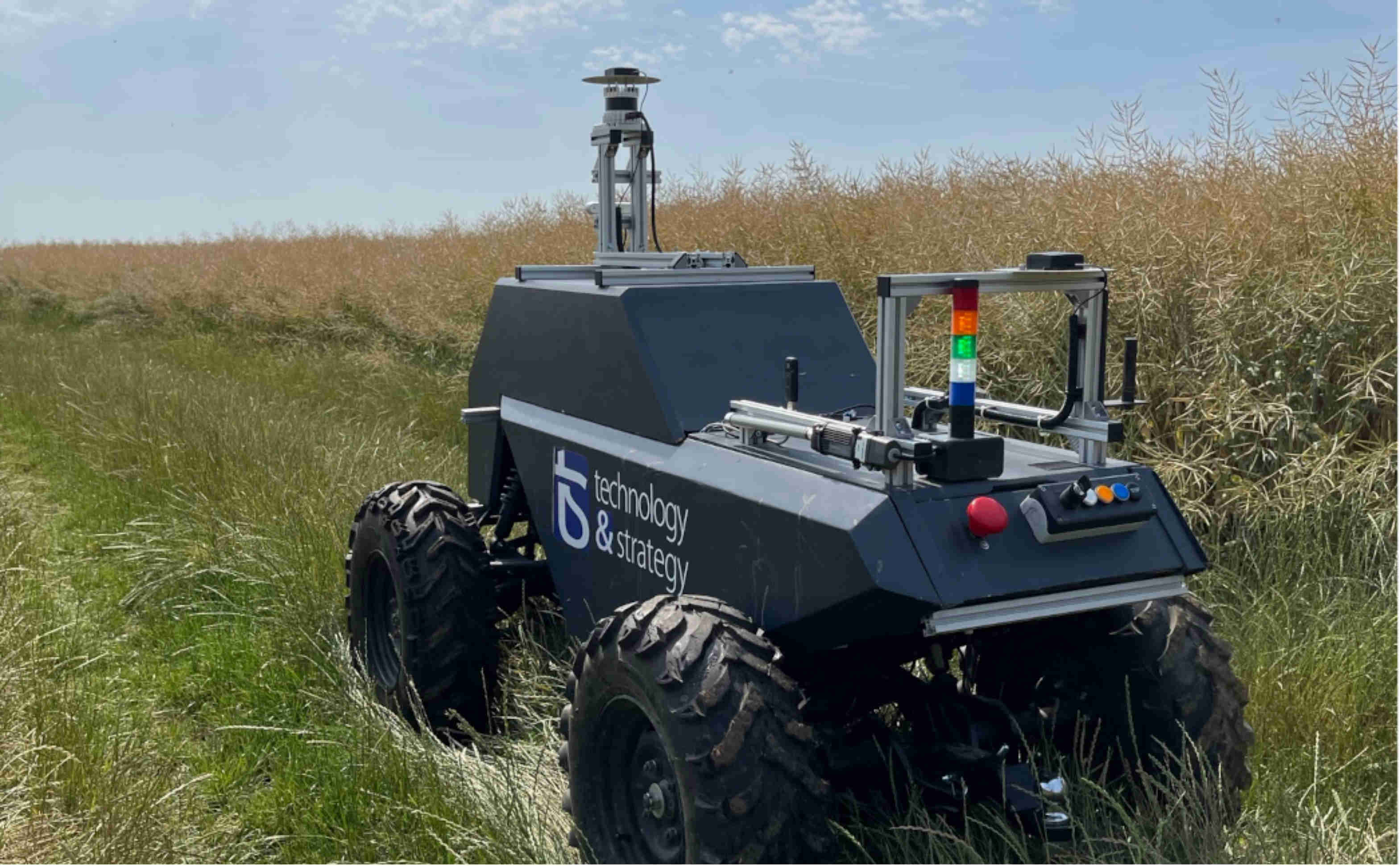
Figure 1: Autonomous plateform navigating through an agricultural field. Tall grass, as well as crops, protrude into the path, forming potential obstacles the robot has to collide with. As such, any system working in such conditions must be able to assess the severity of each collision.

The necessity for a high level of safety in field deployment is paramount, both for the crops themselves and for pedestrians. A fundamental aspect of ensuring safe and resilient navigation is the development of a comprehensive understanding of the surrounding environment. It is imperative that UGVs are aware of any potential danger or lack of sufficient understanding of the surrounding unstructured environment. Furthermore, UGVs should not halt abruptly at every blade of grass seen by the sensors. As such, one must achieve a compromise between security and autonomy.

To address these constraints, it is crucial to identify elements with which the UGV can interact safely. Range measurements are crucial for understanding the environment’s geometry. Additionally, while traditional color cameras can identify scene elements, emerging sensors such as multi-spectral cameras provide higher spectral resolution and more detailed scene information, especially in vegetal environments. Research on leaf chlorophyll content [3] has demonstrated that high reflectance in near-infrared (NIR) bands is indicative of chlorophyll-containing plants. This spectral feature has led to the development of vegetation indices for detecting and monitoring plant health [4]. As such, the advent of multi-spectral cameras offers valuable new data to improve traversability analysis.

In this paper, we propose a physics-based traversability analysis, able to determine whether an element can be traversed or must be avoided by a UGV in an agricultural environment. We propose a novel method that integrates depth and spectral modalities to create a mass density-augmented map by considering the semantic nature of objects within the UGV’s path, aided by precise, non-data-driven vegetation detection. This map is then used to evaluate potential paths in terms of the resulting loss of velocity. The contributions presented in this article are

1. the definition of a new traversability criterion and its physical interpretation for unstructured vegetal environments using emerging sensors; and

2. a quantitative evaluation of vegetation segmentation methods.

II Related work

The concept of traversability analysis has been extensively reviewed in the academic literature. [5] define the objectives of traversability analysis as determining whether a UGV can successfully navigate a path, or doing so while optimizing factors such as travel time or energy consumption. To achieve this goal, the surroundings are modeled during the environmental perception task. This model is used to assess navigation risks and provide crucial information for optimal and safe path planning. [6] classify traversability methods into three categories: vision-based, geometry-based, or hybrid, depending on the exteroceptive modality employed. The majority of methods rely on visual data. Furthermore, [7] highlight the necessity for UGVs to have access to 6 Degrees of Freedom (DoF) pose information and large datasets to train data-driven solutions.

In a structured environment, [8] proposed to generate a 2.5D map by fusing data from both a LiDAR and a camera. Through the application of belief theory, it not only represents the static surroundings but also identifies dynamic objects. In contrast, unstructured environments present greater challenges. [9] proposed fusing height and color data with the UGV velocity to generate an environmental cost grid for offroad application. Their approach is AI-based, utilizing a combination of a convolutional neural network (CNN) and a multilayer perceptron (MLP). This enables more nuanced and diverse navigation behaviors compared to traditional baselines, as vehicle velocity is integrated into the decision-making process. While most map-based approaches describe the environment with navigation costs or physical modeling (e.g., occupancy probability, slope, or ground roughness), [10] introduced a novel criterion based on UGV physics. To evaluate traversability, the environment is modeled in terms of the appropriate speeds for UGVs to navigate specific cells, employing an AI-driven solution. Both methods from [9] and [10] require a setup phase to train the AI model for risk estimation in navigating the environment. However, assessing the risk of traversing impassable areas—such as mud, which poses a sinking hazard, or crops that must be avoided—remains challenging without a highly realistic simulator. Moreover, the success of data-driven segmentation methods strongly depends on the quality, quantity, and diversity of training data [11], making this approach unsuitable for security and environmental protection applications. To address AI’s safety limitations, this paper proposes the use of a model-based semantic segmentation approach.

In difficult environments, relying on a single criterion may be insufficient. For example, in flat terrain like an orchard, speed constraints can provide an effective solution. However, in hillside vineyards, the risk of rollover due to slope increases. [12] proposed a multi-criteria traversability approach. Factors such as slope, ground roughness, and steps are evaluated to create a multi-layered, risk-aware cost grid. The effectiveness of their approach has been demonstrated through field trials conducted in magma tubes and an abandoned metro line. However, one may wonder whether the criteria previously described are able to discern passable elements.

Indeed, the dense vegetation, common during spring and summer in agricultural environments, can hinder the effectiveness of traversability analysis. Vegetation obstructs visual features and introduces additional geometric information that must be disregarded. Being able to detect this vegetation would allow for the integration of its crossability into the traversability analysis. Most of the UGVs visual data currently comes from grayscale or color cameras. However, these sensors have inherent limitations, as the light spectrum extends well beyond visible light, and the three-channel input is insufficient to capture its full complexity. Spectral analysis offers a more comprehensive approach to vision, and multispectral cameras help to address this shortcoming. The use of spectral distances, as discussed by [13] for satellite image classification, has been widely studied, with applications in detecting crops, concrete, and water. These methods assess how closely spectral measurements align with a reference profile. Additionally, green vegetation absorbs red light while reflecting near-infrared (NIR) radiation [3]. As noted by [4], vegetation indices are employed to monitor these spectral bands, providing insights into plant health. In the work of [14], vegetation indices were utilized for vegetation detection, specifically comparing indices based on visible light for segmentation tasks. The Modified Green Red Vegetation Index (MGRVI) demonstrated the best performance in segmenting green plants. Furthermore, Otsu and K-Means binarization algorithms were evaluated, with K-Means delivering superior results in most scenarios. Vegetation segmentation using data-driven methods has also been explored. [15] introduced WeedNet, a segmentation model that employs a CNN with visible and NIR inputs. The network classifies weeds, crops, and background, achieving an F1 score of 0.8 and an Area Under the Curve (AUC) of 0.78 in classification metrics, with applications in weed control. For navigation tasks, [16] developed a segmentation network to detect trails in unstructured environments using a multispectral camera to enhance navigation. This approach achieved an Intersection over Union (IoU) score of 0.85 for vegetation detection.

Few studies have been conducted on the application of spectral measurements for proximity detection. [17] proposed fusing vegetation indices with LiDAR depth data for obstacle detection. Superpixel generation on the NDVI image facilitates the detection of non-plant elements. A Support Vector Machine (SVM) classifier is then applied to categorize obstacles based on various geometric and visual features. However, this method is measurement-based. In a map-based approach, false detections could be filtered out by leveraging prior knowledge, due to most of the environment being static over time. To build an environmental model, [18] combined multispectral and LiDAR measurements into a 3D map of the environment, augmented with the Normalized Difference Vegetation Index (NDVI). These 3D maps are subsequently used to monitor the health of plantations, as well as for fruit detection and counting operations using data-driven methods. In this paper, a similar map is generated to conduct traversability analysis based on the semantic segmentation of vegetation within the environment.

Section III introduces a traversability index that accounts for the semantic characteristics of scene elements to estimate their traversability. This method addresses the issue of false detections caused by dense vegetation in agricultural environments.

III Map-based Traversability Estimation

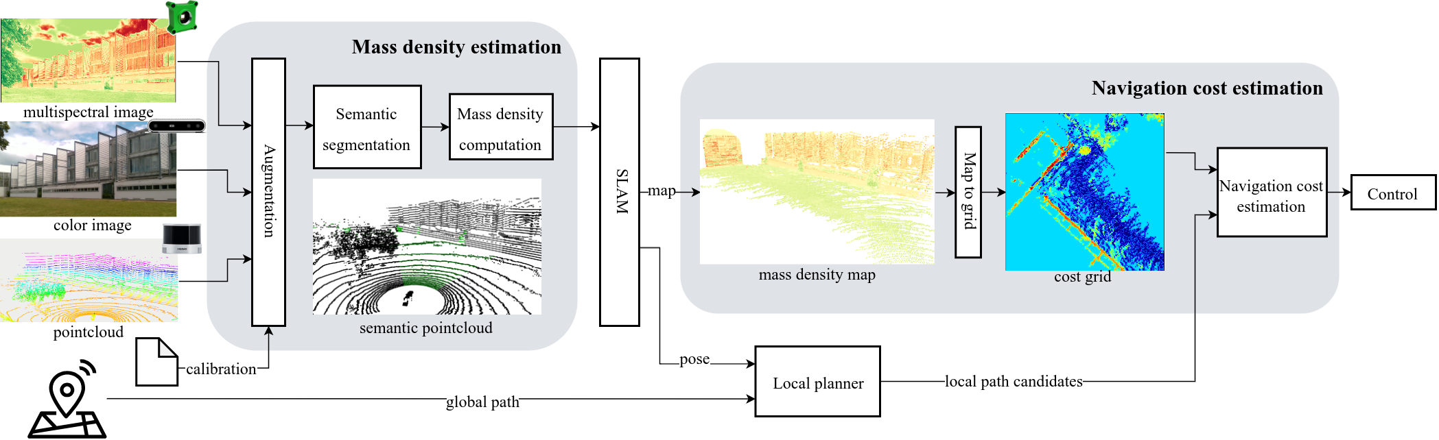
Figure 2: Traversability analysis flow: Multispectral images are fused with LiDAR data to produce an augmented point cloud, which serves as the basis for semantic segmentation. Mass density is calculated for each depth measurement, updating the 3D environmental map. This is then converted into a 2D traversability grid. Ultimately, potential paths are assessed, and the safest one is chosen.

The objective of the proposed method is to estimate a path navigation cost by computing the potential loss of velocity that would be experienced by the UGV traversing it. Figure 2 illustrates the traversability analysis pipeline. Initially, the spectral measurements obtained from the camera are projected into the point cloud of the LiDAR. A semantic segmentation of the environment is conducted using spectral measurements. A mass density is estimated for each LiDAR point in the camera’s field of view, on the basis of the probabilities of belonging to a given semantic class. The augmented point cloud is then filtered and stored within a 3D map, before being projected onto a 2D grid in order to estimate the traversability of the terrain. The loss of velocity for a given trajectory is estimated. Local paths leading to a larger velocity loss are rejected, and thus a safe trajectory is selected.

III-A Raw data processing

The first step is to process the raw sensor data to derive a spectrally-enhanced depth measurement. After performing the necessary calibrations, the LiDAR data is projected onto the camera measurements. We refer to the outcome of this procedure as the spectrally augmented point cloud. In order to fuse spectral and spatial information on a 3D map, three calibrations are required:

Intrinsic calibration

estimates the distortion coefficients of the optics, the focal lengths and the optical center coordinates forming intrinsic matrix $\bm{K}\in\mathbb{R}^{3\times 4}$ of each camera.

Extrinsic calibration

identifies the relative pose between each sensor and provides a transformation matrix defined by $\bm{T}\in SE(3)$.

Spectral calibration

[19] proposed a calibration procedure to establish a connection between reflectance, i.e., the physical material properties that determine how light is reflected, and the light intensity sensed by the camera. This step leads to multispectral image illustrated in Figure 2. The conversion is achieved through the use of a linear system model. The spectral reflectance vector, denoted as $\bm{r}\in\mathbb{R}^{m}$, is estimated based on the corresponding spectral intensity vector $\bm{i}\in\mathbb{R}^{n}$, using the spectral calibration matrix $\bm{M}\in\mathbb{R}^{m\times n}$, for each pixel of the camera image. The reflectance vector is defined as

$$\bm{r}=\bm{M}\bm{i}.$$ (1)

From this, the lidar point cloud is projected on the image frame using

$$\bm{p}_{\text{image}}=\bm{K}\bm{T}\bm{p}_{\text{lidar}},$$ (2)

where $\bm{p}_{\text{lidar}}\in\mathbb{R}^{4}$ and $\bm{p}_{\text{image}}\in\mathbb{R}^{3}$ denotes the depth data measured by the LiDAR in their respective frames. As such, the LiDAR point cloud is augmented with spectral information from the camera, that will be used in the following to estimate a mass density map. This process is illustrated in Figure 2, where it is denoted as augmentation.

III-B Mass density map generation

Using the spectrally augmented point cloud, the aim of this section is to estimate the mass density of the environment. Therefore, we define the mass density augmented point cloud as a set of vectors of the form $[x,y,z,d_{m}]^{T}$, where $d_{m}\in\mathbb{R}_{\geq 0}$ denotes the associated mass density. This step is denoted as Mass density computation in Figure 2. For this, we propose a data-driven approach: each of the $n$ semantic classes, $c_{i}$, is associated with a reference mass density $d_{m}(c_{i})$. Furthermore, to address the inherent uncertainties, the mass density is modeled as a random variable. The mass density is computed as the expected value alongside the possible obstacles classes probabilities $p(c_{i})$, as

$$\mathbb{E}[d_{m}] =\sum_{i=1}^{n}d_{m}(c_{i})\cdot p(c_{i}|s)$$ (3)

$$=\frac{\sum_{i}d_{m}(c_{i})p(s|c_{i})}{\sum_{i}p(s|c_{i})},$$

where $s$ is the semantic measurement, and $p(c_{i}|s)$ are the confidence on the measurements. Such values can be either input in the framework, or learned from an annotated dataset.

Once the 4D point cloud is processed, it is transformed into a 3D map to be used for traversability analysis. The 3D map is generated by aggregating the 4D measurements into a voxel grid, converting them into the world frame. The sensor poses is determined using the SLAM LiDAR solution from [20]. Next, the 3D map is converted into a 2D grid to assess navigation costs. This process is depicted in Figure 2 as Map to grid. This is done by flattening the map, where ground points are filtered using the RANSAC algorithm [21], along with points above the UGV’s height. The mass density grid is initialized with the UGV mass value and is later filled with the maximum mass density value from the corresponding Z-axis column. As such, a 2D grid map with mass density information is generated, that is used in the next section to estimate the loss of velocity a robot would undergo given a path in the environment.

III-C Velocity loss evaluation

Using the mass density grid, we derive a physics-based formulation for traversability, relying on the loss of velocity due to navigation in nonempty space. This step is designated as Navigation costs estimation in Figure 2. Assuming inelastic collisions, the final velocity $v_{R}^{f}$ of the UGV is computed as

$$v_{R}^{f}=\frac{m_{R}}{m_{R}+m_{i}}v_{R}\Leftrightarrow v_{R}^{f}=\alpha v_{R},$$ (4)

where $v_{R}$ is the initial velocity of the UGV, $m_{R}$ the mass of the robot, and $m_{i}$ the mass of the $i$th obstacle.

From this, we model the environment as a collection of infinitesimal particles of area $\Delta a\to 0$. Given a path $\mathcal{P}\subset\mathbb{R}^{2}$ crossing a total area $A$, the velocity coefficient $\alpha$ of the robot is given by

$$\alpha=\prod_{i=1}^{N}\frac{m_{R}}{m_{R}+d_{m}(i)\Delta a},$$ (5)

assuming colliding with $N$ particles of size $\Delta a$ such that $N\Delta a=A$. Note that free space is modeled as a particle of null mass density. From this, with the particle area $\Delta a$ tending towards zero, the equation becomes

$$\alpha =\lim\limits_{\Delta a\to 0}\prod_{i=1}^{A/\Delta a}\frac{m_{R}}{m_{R}+d_{m}(i)\Delta a}$$ (6)

$$=\exp{\left(-\frac{1}{m_{R}}\int_{\mathcal{P}}d_{m}(a)da\right)},$$

where $d_{m}(a)$ denoted the local mass density at the given position in the environment. As such, for infinitesimal particles, Equation 7 compute the ratio of lost velocity is undergoing the path $\mathcal{P}$. In the case of a grid map in which the mass density is constant inside each cell, the equation can be simplified to

$$\alpha =\exp{\left(-\frac{1}{m_{R}}\sum_{c_{i}\in\mathcal{P}}d_{m}(i)a_{c}\right)},$$ (7)

where $a_{c}$ is the area of a grid cell. One can note that assuming infinitesimal collisions result in a lower bound on the loss of velocity, meaning that we will always overestimate the risk for one path.

To summarize, the environment is modeled through the multimodal fusion of LiDAR and cameras, as described in Equation 2. As the UGV navigates, the grid is continuously updated to represent the mass density of surrounding elements using Equation 3. This grid is subsequently used to evaluate routes candidates using Equation 7, allowing the selection of the safest path. This method enables the environment to be physically characterized by the expected loss of velocity by crossing a specific region. As such, the ratio of velocity $\alpha$ will be used as the navigation cost. In the following section, we will qualitatively assess this approach and quantitatively evaluate a non-data-driven vegetation semantic segmentation solution.

IV Evaluations

In this section, we outline the setup employed for evaluating the proposed method. Next, we assess the performance of the semantic segmentation indices, followed by an offline test of our traversability analysis solution using recorded data.

IV-A Experimental Setup

A teleoperated platform was equipped with a Hesai Pandar XT-32 LiDAR, a Silios CMS-V VNIR multispectral camera, and an Intel Realsense D415 stereoscopic camera. The VNIR camera provided 8 spectral measurements from $550\text{\,}\mathrm{nm}$ to $830\text{\,}\mathrm{nm}$, in addition to a panchromatic (PAN) measurement. The stereoscopic camera provided 3 channels of RGB measurements. Data are collected using this mobile measurement bench, enabling us to evaluate our traversability analysis solution offline. As illustrated in Figure 3, one of the environments explored was a park with tall grass, untrimmed trees and winding paths. Buildings and static pedestrians are present throughout the navigation. The weather was mild during the recordings.

IV-B Semantic segmentation performance

In Section III-B, we presented a generic way to estimate the mass density of the environment using semantic classes. As such, the quality of this estimate rely heavily on the level of accuracy on the segmentation. The following section presents a thorough quantitative evaluation of vegetation indices and spectral distance performances, highlighting their performance to differentiate vegetation from other objects. The evaluation is conducted using a manually annotated 3D dataset, where spectral information was fused with a 3d point cloud. Each point on the map is labeled with one of the following classes: Grass, Track, Vegetation, Building, Pedestrian, Obstacle or Other. An example of the annotation and spectral measurements is depicted in Figure 3. In total, $6\text{\,}228\text{\,}592\text{\,}$ points were annotated for a total covered area of $2515\text{\,}{\mathrm{m}}^{2}$, consisting of off-road environments.

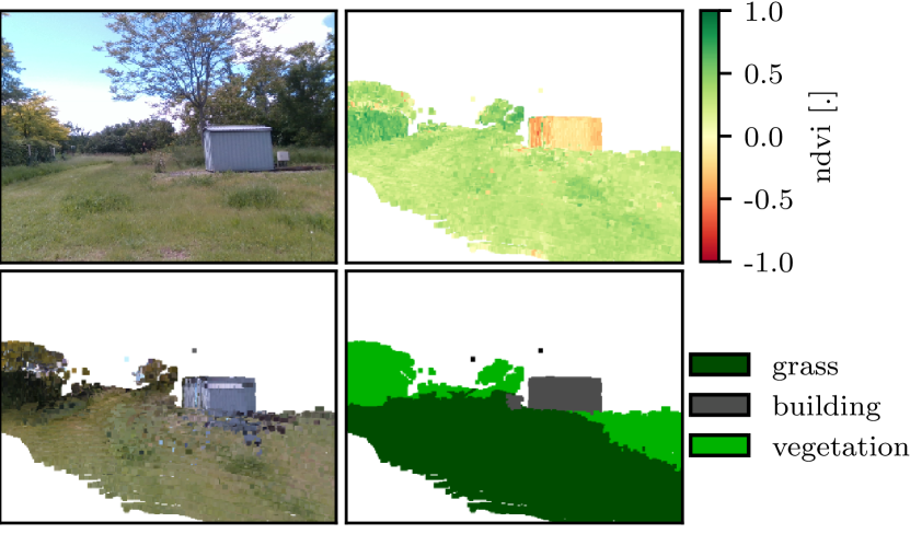
Figure 3: Augmented 3D maps of a park environment, consisting of tall grass, bushes, trees and a small shack. Top Left: Color camera’s image from the scene; Top Right: ndvi colorized 3D map; Bottom Left: visible light colorized 3D map; Bottom Right: Manually annotated 3D map

The present study focuses on the vegetation detection: a macro-class designated Plants is defined, encompassing both the Vegetation and Grass classes, while all other classes are included under the $\neg\texttt{Plants}$ macro-class.

In the following, we evaluate the most popular metrics to detect and quantify the vegetation. Namely, the Modified Green-Red Vegetation Index (mgrv), Green Leaf Index (gli), Modified Photochemical Reflectance Index (mpr), Red-Green-Blue Vegetation Index (rgbvi), Excess of Green (exg), Excess of Red (exr), Vegetative (veg), Normalized Difference Vegetation Index (ndvi), and Enhanced Vegetation Index (evi) [4], are evaluated. Additionally, the spectral distances, such as Euclidean Distance (ed), Bray-Curtis Distance (bc), and Spectral Angle (sa) [13, 22] are also compared. The reference reflectance profiles used for the computation of spectral distances were extracted from the annotated spectral maps for each class by averaging the spectral measurements. These profiles consist of 29 wavelengths, ranging from $550\text{\,}\mathrm{nm}$ to $830\text{\,}\mathrm{nm}$, and are presented in Figure 4.

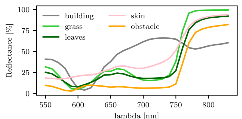
Figure 4: Reflectance profiles of several elements of agricultural environment

The segmentation procedure is described as follows: the vegetation index and spectral distance are applied to the spectral augmented maps. Subsequently, a binarization step is conducted using the Otsu algorithm [23] to segment vegetation with a dynamic threshold. The Intersection over Union (IoU), Precision (Prec.), Accuracy (Acc.), Recall (Rec.), F1 score, Specificity (Spec.) and computation duration $\Delta t$ are compared for each vegetation segmentation method in Table I. An AMD Ryzen 7 5000 series CPU is used for the computational duration measures.

TABLE I: Plants semantic segmentation performance

Index	IoU	Prec.	Rec.	Acc.	F1	Spec.	$\Delta t$ [ms]
mgrv	0.54	0.94	0.56	0.62	0.70	0.84	169.5
gli	0.42	0.97	0.43	0.53	0.59	0.94	107.5
mpri	0.49	0.94	0.51	0.58	0.66	0.88	60.3
rgbvi	0.68	0.87	0.76	0.71	0.81	0.53	148.3
exg	0.56	0.98	0.57	0.64	0.72	0.94	82.9
exr	0.33	0.78	0.37	0.41	0.50	0.57	64.1
exgr	0.64	0.89	0.70	0.69	0.78	0.63	138.8
veg	0.80	0.84	0.94	0.81	0.89	0.27	194.8
evi	0.56	0.99	0.56	0.64	0.72	0.98	104.0
ndvi	0.91	0.99	0.92	0.93	0.95	0.94	67.8
sa	0.69	0.79	0.84	0.69	0.81	0.05	883.7
bc	0.66	0.95	0.69	0.72	0.80	0.85	1589.4
ed	0.90	0.96	0.93	0.91	0.95	0.84	430.1

As such, the most reliable method for identifying vegetation in proximate detection applications is the ndvi. However, its response is dependent on the wavelength of only two specific frequencies, since the ndvi is computed as

$$\text{ndvi}=\frac{i_{810}-i_{650}}{i_{810}+i_{650}},$$ (8)

where the intensity of light at a specific wavelength $\lambda$ nm is denoted as $i_{\lambda}$. False positives are likely in the case of certain elements with similar reflectance in the red and NIR bands (e.g., plastics and textiles). Pedestrians represent a small portion of the dataset, so false detections related to their clothing have a negligible effect on the overall performance results presented. Spectral distance, such as the spectral angle, measures the consistency of a measurement with respect to a reference profile over a much higher resolution. At the expense of processing time, this allows for greater robustness to local similarities in the analyzed light spectrum. As such, when deadline with more complex environments where there is a thinner granularity than only differentiating between vegetation and non-vegetation, these metrics would prove themselves more robust. Such metrics will be investigated in future works.

Given the results in Table I, the normalized ndvi index is used to generate belonging probabilities of Plants class in Equation 3.

IV-C Navigation costs estimation analysis

In this section, we present an application of our method. For simplicity, we focus on only two classes that are Plants and $\neg\texttt{Plants}$, where future works will focus on using more classes for safe navigation. It is imperative that the Other class is not navigable; therefore, the concrete mass density is set for this class [24]. In contrast, the Plants class permits navigation. The respective mass densities $d_{m}(\texttt{Plants})$ and $d_{m}(\neg\texttt{Plants})$ are set to $20\text{\,}\mathrm{kg}\text{\,}{\mathrm{m}}^{-2}$ and $2400\text{\,}\mathrm{kg}\text{\,}{\mathrm{m}}^{-2}$. The UGV mass is set to $250\text{\,}\mathrm{kg}$. The cost grid is next extracted from the mass density-augmented map, as described in Section III.

Figure 5 illustrates an example of navigation. In this scenario, a path-following solution presents the UGV with a series of potential local paths, each of which offers a different route to reach the desired objective. Each of these routes is then evaluated using the navigation cost function, which is applied to the mass density grid. The environment is characterized by the presence of high grass, dense vegetation (e.g., bushes, trees) and buildings, as illustrated on the semantic grid. The UGV’s local planner generates seven candidate paths (color pixels) over the cost grid (gray pixels).

The path p1 guides the vehicle through a grove of trees, with a navigation cost of ($\alpha_{1}=0.4$). This results in a significant reduction in speed due to the collision with the substantial vegetation. Path p7 directs the UGV to an uncharted region. The navigation cost is ($\alpha_{7}=0.7$) due to the grid initialization and the unknown nature of the objects it contains. Ultimately, path p4 traverses exclusively through regions with null density mass. As shown in the label grid, the path is comprised solely of grass, which is a component of the ground. The navigation cost of p4 is ($\alpha_{4}=0.9$), indicating that the UGV will not experience a loss of speed when navigating this route. The local planner selected this path over the other candidates.

This method is based on semantic understanding of the environment. It can be employed in diverse environments settings and extended with different semantic classes. Furthermore, it can be adapted to any UGV’s size, from a lawnmower to a tractor, by setting the appropriate mass value $m_{R}$. Finally, the loss velocity coefficient $\alpha$ used to evaluate a candidate path can be derived to estimate more complex metrics, such as the loss of kinetic energy over a path.

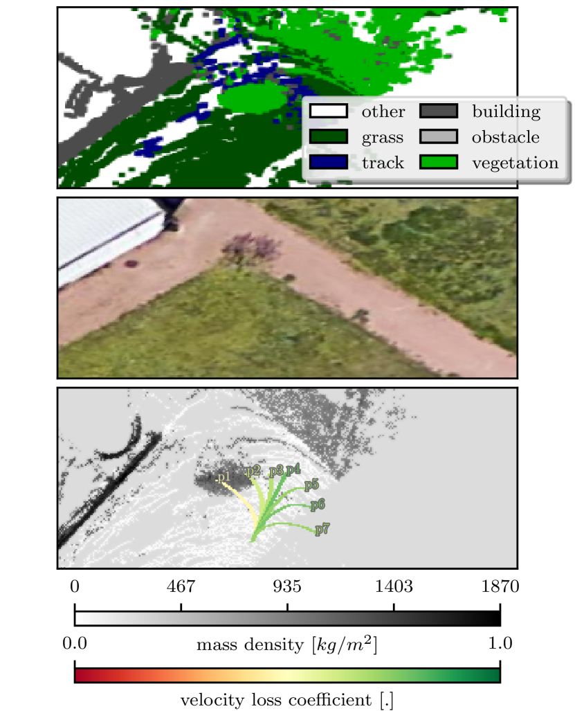
Figure 5: Local planning candidates evaluated based on the mass density grid. Semantic grid (top) and satellite view (middle) illustrate the environmental configuration during the run (middle). The local paths over the cost grid (bottom) illustrate navigation costs of each candidate. A coefficient of $1$ means no loss of velocity, thus a safe path, whereas a coefficient of $0$ means a collision resulting in the total stop of the robot.

V Conclusion

In this paper, we presented a novel traversability analysis method specifically designed for Unmanned Ground Vehicle (UGV) navigation in agricultural environments. The proposed approach constructs a representation of the environment that incorporates both impassable obstacles and crossable elements within the scene.

A quantitative evaluation of algorithms for vegetation segmentation was conducted, demonstrating that the use of the Normalized Difference Vegetation Index (ndvi) yields the most effective results in terms of detection accuracy and computational efficiency.

We provided an example of the use of our framework for traversability analysis, showing that the robot is able to differentiate between dangerous and safe collisions. The approach can be adapted to various UGV models, allowing for flexibility in how obstacles are defined based on specific vehicle requirements.

For future work, additional semantic classes could be explored for density map estimation, utilizing either the spectral angle distance, or a data-driven approach with appropriate safeguards. Furthermore, integrating the mass index into a multi-layer grid would be advantageous, as it would enable the inclusion of additional features to enhance the traversability estimation. These features could include ground slope, height map, and other relevant characteristics.

References

- [1] Spyros Fountas et al. “Agricultural Robotics for Field Operations” Number: 9 Publisher: Multidisciplinary Digital Publishing Institute In Sensors 20.9, 2020, pp. 2672 DOI: 10.3390/s20092672
- [2] Roland Lenain, Julie Peyrache, Alain Savary and Gaëtan Séverac “Agricultural robotics: part of the new deal?: FIRA 2020 conclusions” éditions Quae, 2021 URL: https://library.oapen.org/handle/20.500.12657/51620
- [3] Anatoly Gitelson, Yuri Gritz and Mark Merzlyak “Relationships between leaf chlorophyll content and spectral reflectance and algorithms for non-destructive chlorophyll assessment in higher plant leaves” In Journal of plant physiology 160, 2003, pp. 271–82 DOI: 10.1078/0176-1617-00887
- [4] Bannari Abderrazak, D. Morin, F. Bonn and Alfredo Huete “A review of vegetation indices” In Remote Sensing Reviews 13.1, 1996, pp. 95–120 DOI: 10.1080/02757259509532298
- [5] Mohamed Benrabah, Charifou Orou Mousse, Elie Randriamiarintsoa, Roland Chapuis and Romuald Aufrère “A Review on Traversability Risk Assessments for Autonomous Ground Vehicles: Methods and Metrics” Number: 6 Publisher: Multidisciplinary Digital Publishing Institute In Sensors 24.6, 2024, pp. 1909 DOI: 10.3390/s24061909
- [6] Semih Beycimen, Dmitry Ignatyev and Argyrios Zolotas “A comprehensive survey of unmanned ground vehicle terrain traversability for unstructured environments and sensor technology insights” In Engineering Science and Technology, an International Journal 47, 2023, pp. 101457 DOI: 10.1016/j.jestch.2023.101457
- [7] Paulo Borges et al. “A Survey on Terrain Traversability Analysis for Autonomous Ground Vehicles: Methods, Sensors, and Challenges” In Field Robotics 2.1, 2022, pp. 1567–1627 DOI: 10.55417/fr.2022049
- [8] Hind Laghmara, Thomas Laurain, Christophe Cudel and Jean-Philippe Lauffenburger “2.5D Evidential Grids for Dynamic Object Detection” In 2019 22th International Conference on Information Fusion (FUSION), 2019, pp. 1–7 DOI: 10.23919/FUSION43075.2019.9011417
- [9] Mateo Guaman Castro et al. “How Does It Feel? Self-Supervised Costmap Learning for Off-Road Vehicle Traversability” In 2023 IEEE International Conference on Robotics and Automation (ICRA), 2023, pp. 931–938 DOI: 10.1109/ICRA48891.2023.10160856
- [10] Xiaoyi Cai, Michael Everett, Jonathan Fink and Jonathan P. How “Risk-Aware Off-Road Navigation via a Learned Speed Distribution Map” In 2022 IEEE/RSJ International Conference on Intelligent Robots and Systems (IROS), 2022, pp. 2931–2937 DOI: 10.1109/IROS47612.2022.9982200
- [11] Liangkai Liu et al. “Computing Systems for Autonomous Driving: State of the Art and Challenges” Conference Name: IEEE Internet of Things Journal In IEEE Internet of Things Journal 8.8, 2021, pp. 6469–6486 DOI: 10.1109/JIOT.2020.3043716
- [12] David D. Fan et al. “STEP: Stochastic Traversability Evaluation and Planning for Risk-Aware Off-road Navigation” In Robotics: Science and Systems XVII 17, 2021 DOI: 10.15607/RSS.2021.XVII.021
- [13] “Image Classification Methodologies” In Remote Sensing Digital Image Analysis: An Introduction Berlin, Heidelberg: Springer, 2006, pp. 295–332 DOI: 10.1007/3-540-29711-1˙11
- [14] Jean Santos, Jocival Dias Junior, André Backes and Maurício Escarpinati “Segmentation of Agricultural Images using Vegetation Indices:” In Proceedings of the 16th International Joint Conference on Computer Vision, Imaging and Computer Graphics Theory and Applications SCITEPRESS - ScienceTechnology Publications, 2021, pp. 506–511 DOI: 10.5220/0010325005060511
- [15] Inkyu Sa et al. “weedNet: Dense Semantic Weed Classification Using Multispectral Images and MAV for Smart Farming” Conference Name: IEEE Robotics and Automation Letters In IEEE Robotics and Automation Letters 3.1, 2018, pp. 588–595 DOI: 10.1109/LRA.2017.2774979
- [16] Abhinav Valada, Gabriel L. Oliveira, Thomas Brox and Wolfram Burgard “Deep Multispectral Semantic Scene Understanding of Forested Environments Using Multimodal Fusion” Series Title: Springer Proceedings in Advanced Robotics In 2016 International Symposium on Experimental Robotics 1 Cham: Springer International Publishing, 2017, pp. 465–477 DOI: 10.1007/978-3-319-50115-4˙41
- [17] Nan Zou, Zhiyu Xiang and Jiapeng Zhang “Multi-spectrum superpixel based obstacle detection under vegetation environments” In 2017 IEEE Intelligent Vehicles Symposium (IV), 2017, pp. 1209–1214 DOI: 10.1109/IVS.2017.7995877
- [18] Thibault Clamens et al. “Real-time Multispectral Image Processing and Registration on 3D Point Cloud for Vineyard Analysis:” In Proceedings of the 16th International Joint Conference on Computer Vision, Imaging and Computer Graphics Theory and Applications SCITEPRESS - ScienceTechnology Publications, 2021, pp. 388–398 DOI: 10.5220/0010266203880398
- [19] Sumera Sattar, Pierre-Jean Lapray, Lyes Aksas, Alban Foulonneau and Laurent Bigué “Snapshot spectropolarimetric imaging using a pair of filter array cameras” Publisher: SPIE In Optical Engineering 61.4, 2022, pp. 043104 DOI: 10.1117/1.OE.61.4.043104
- [20] Kenji Koide, Jun Miura and Emanuele Menegatti “A portable three-dimensional LIDAR-based system for long-term and wide-area people behavior measurement” Publisher: SAGE Publications In International Journal of Advanced Robotic Systems 16.2, 2019 DOI: 10.1177/1729881419841532
- [21] Martin A. Fischler and Robert C. Bolles “Random sample consensus: a paradigm for model fitting with applications to image analysis and automated cartography” In Commun. ACM 24.6, 1981, pp. 381–395 DOI: 10.1145/358669.358692
- [22] F.. Kruse et al. “The spectral image processing system (SIPS)—interactive visualization and analysis of imaging spectrometer data” In Remote Sensing of Environment 44.2, Airbone Imaging Spectrometry, 1993, pp. 145–163 DOI: 10.1016/0034-4257(93)90013-N
- [23] Nobuyuki Otsu “A Threshold Selection Method from Gray-Level Histograms” Conference Name: IEEE Transactions on Systems, Man, and Cybernetics In IEEE Transactions on Systems, Man, and Cybernetics 9.1, 1979, pp. 62–66 DOI: 10.1109/TSMC.1979.4310076
- [24] “NF EN 206/CN” P18-325/CN: AFNOR, 2014 URL: https://www.boutique.afnor.org/fr-fr/norme/nf-en-206-cn/beton-specification-performance-production-et-conformite-complement-nationa/fa185553/1463