Inter–disks inversion surfaces

Abstract

We consider a counter–rotating torus orbiting a central Kerr black hole (BH) with dimensionless spin $a$, and its accretion flow into the BH, in an agglomerate of an outer counter–rotating torus and an inner co–rotating torus. This work focus is the analysis of the inter–disks inversion surfaces. Inversion surfaces are spacetime surfaces, defined by the condition $u^{\phi}=0$ on the flow torodial velocity, located out of the BH ergoregion, and totally embedding the BH. They emerge as a necessary condition, related to the spacetime frame–dragging, for the counter–rotating flows into the central Kerr BH. In our analysis we study the inversion surfaces of the Kerr spacetimes for the counter–rotating flow from the outer torus, impacting on the inner co–rotating disk. Being totally or partially embedded in (internal to) the inversion surfaces, the inner co–rotating torus (or jet) could be totally or in part “shielded”, respectively, from the impact with flow with $au^{\phi}<0$. We prove that, in general, in the spacetimes with $a<0.551$ the co–rotating toroids are always external to the accretion flows inversion surfaces. For $0.551<a<0.886$, co–rotating toroids could be partially internal (with the disk inner region, including the inner edge) in the flow inversion surface. For BHs with $a>0.886$, a co–rotating torus could be entirely embedded in the inversion surface and, for larger spins, it is internal to the inversion surfaces. Tori orbiting in the BH outer ergoregion are a particular case. Further constraints on the BHs spins are discussed in the article.

I Introduction

The spacetime frame-dragging influences the accretion processes acting, in particular, on the flows from counter–rotating accretion disks, where the Lense–Thirring effect acts on the accretion flows with an initial counter–rotating component, reversing its rotation direction, i.e. the toroidal component of the velocity $u^{\phi}$ in the proper frame along its trajectory. In this analysis we focus on counter–rotating flows accreting into a central Kerr Black Hole (BH). The flow, assumed to be free–falling into the central attractor, inherits some properties of the counter–rotating accreting configurations. Therefore, because of the frame–dragging, the flow trajectory is characterized by the presence of flow inversion points, defined by the condition $u^{\phi}=\Omega=0$ on the toroidal component of the flow velocity and relativistic angular velocity. All the inversion points are located on a surface, the inversion surface, placed out of the BH outer ergosurface and dependent on the flow specific angular momentum only [1, 2, 3, 4].

In particular we explore an aggregate of toroidal accretion disks orbiting on the equatorial plane of the Kerr BH, composed by an outer counter–rotating disk and a co–rotating inner disk, studying the inversion surfaces of the counter–rotating flows which are accreting onto the central BH. The inner co–rotating disk of the double system, can be embedded, external or partially contained in the spacetimes inversion surfaces (inter–disks inversion surfaces), according to the BHs spins and the counter–rotating flows specific angular momentum. Our analysis fixes the more general conditions where a co–rotating accretion disks can impact with materials with $au^{\phi}<0$ (where $a>0$ is the BH spin). The disks embedded in an inversion surface will be completely shielded from impact with particles (and photons) with $u^{\phi}<0$, accreting into the central Kerr BH.

It is important to note that the inversion surface (defined as the loci of the vanishing toroidal flow velocity) can be contained in the region defined by the surface separating the co-rotating and counter-rotating component, depending on whether the co-rotating disks are contained inside the inversion surface or not. In this work we analyse the relation between these surfaces depending on the BH spin and some tori parameters, leading to three different scenarios. The toroids can be 1. embedded in an inversion surface; 2. located out of the inversion surface or 3. crossing the inversion surfaces in particular points being partially contained in the inversion surface. Our finding therefore ultimately constrain the case when the inner co–rotating disk can be replenished with matter (and photons) having $au^{\phi}<0$ which is accreting into the central BH or, viceversa when the counter–rotating flow impacts on the co–rotating disk with $au^{\phi}>0$, influencing the disk dynamics, combining with the co–rotating accreting flows and eventually affecting the co–rotating disk inner edge (and, connected with the physics of the inner edge, the launching of materials in jets along the BH axis). This situation will be constrained according to the flow parameters and the BH dimensionless spin $a$.

Counter–rotating accretion flows are well known in the BH Astrophysics. Counter–rotation can also distinguish BHs with or without jets [8, 9]. Counter–rotation of the extragalactic microquasars have been investigated for example also as engines for jet emission, see [23, 15], connected to SWIFT J1910.2 0546 [22], and the faint luminosity of IGR J17091–3624 (a transient X-ray source believed to be a Galactic BH candidate) [21]. (Observational evidence of counter–rotating disks has been also discussed in relation to M87, observed by the Event Horizon Telescope [28].) They can be produced for example during chaotical, discontinuous accretion processes, where aggregates of co–rotating and counter—rotating toroids can be mixed [26, 29, 30, 31, 32, 33]. Therefore they could also appear in binary systems with stellar mass BHs (as in 3C120 [34, 25]), in the Galactic binary BHs [20, 22], and more generally in BH binary system ([24] or [13]). Eventually even misaligned disks with respect to the central BH spin can form in these situations [35, 36, 37, 38, 39, 40, 41, 42, 43]. The Lense–Thirring effect in misaligned disks can be manifested in the Bardeen–Petterson effect, where the BH spin can change under the action of the tori torques, with an originally misaligned torus broken due to the frame–dragging combined to other factors as the fluids viscosity, in a double system as the aggregate considered in this work, composed by an inner co–rotating torus and an counter–rotating outer torus [44, 50, 49, 45, 46, 47, 51, 18, 48, 52, 45].

BHs could accrete from disks having alternately co–rotating and counter–rotating senses of rotation [5]. Hence, more complex scenarios envisaging complicated superimposed sub–structures of counter–rotating and co–rotating materials have been also studied. In [26], for example, a high-resolution axisymmetric hydrodynamic simulation of viscous counter–rotating disks was presented for the cases where the two components are vertically separated or radially separated. A time-dependent, axisymmetric hydrodynamic (HD) simulation of complicated composite counter–rotating accretion disks was studied in [6], where the disks consist of combined counter–rotating and corotating components. (It is worth noting that the accretion rates are increased over that for co–rotating disks–see also [6].) Counter–rotating tori have been modelled also as a counter–rotating gas layer on the surface of a co–rotating disk. Reversals in the rotation direction of an accretion disk, “flip–flop” phase, have been considered to explain state transitions[20].

In this article we will consider an aggregate of co–rotating and counter–rotating toroids. This system has been constrained in [53, 31, 54, 55] and widely discussed in subsequent papers [56, 33, 32, 57, 58, 59, 60, 61, 63]. Evidences of the presence of a toroids agglomerate with an inner co–rotating torus and outer counter–rotating torus has been provided by Atacama Large Millimeter/submillimeter Array (ALMA). It has been assumed that the outer disk could have been formed in recent times from molecular gas falling. The inner disks follows the rotation of the galaxy, whereas the outer disk rotates (in stable orbit) the opposite way. The interaction between counter–rotating disks may enhance the accretion rate with a rapid multiple phases of accretion. The presence of two disks of gas rotating in opposite directions can be pointed out from the observation of gas motion around the BH inner orbits. From methodological view–point, in this work we shall examine a free–falling accretion flow constituted by counter–rotating matter (and photons), and axially symmetric equatorial geometrically thick co–rotating and counter–rotating toroids orbiting on the BH equatorial plane. We use a full General Relativistic Hydrodynamical (GRHD) model, which include proto-jets solutions–[62, 53]. Proto-jets are open HD toroidal configurations, with matter funnels along the BH rotational axis, associated to thick disks, and emerging under special conditions on the fluid forces balance. The focus of this work is the analysis of the inter–disks inversion surfaces, however, for completeness, we shall also discuss the case when one or two of these configurations are proto-jets.

In details the plan of this article is as follows:

The spacetime metric is introduced in Sec. (II). In Sec. (II.1) there are the geodesic equations of motion in Kerr spacetime. Constraints on the flows and orbiting toroids are discussed in Sec. (III). Sec. (III.1) details the geometrical thick accretion disk model in the Kerr spacetime, developing the analytical conditions adopted in the following analysis. The section contains also further notes on the toroids extreme points. In Sec. (IV) the inversion surfaces are introduced. In Sec. (V) we focus on the co–rotating toroids orbiting the central Kerr BH in relation to the spacetime inversion surfaces. Some preliminary aspects are explored in Sec. (V.1), where we investigate the inter–disks inversion surfaces in different Kerr BHs spacetimes, distinguishing BHs classes according to the BH spins and the inversion surfaces properties in the spacetimes of each class. In Sec. (V.2) the inversion surfaces crossing the co–rotating toroids are examined. The crossing with the co–rotating toroids outer edges is addressed in Sec. (V.2.1). The surfaces crossing with the toroids cusps are studied in Sec. (V.2.2), and the case of the inversion surfaces crossing the toroids centers is discussed in Sec. (V.2.3). The surfaces crossing the toroids critical points of pressure and geometrical maxima are the subject of Sec. (V.2.4), while the crossing on planes different from the equatorial is examined in Sec. (V.2.5). Conclusions are in Sec. (VI).

II The spacetime metric

In the Boyer-Lindquist (BL) coordinates $\{t,r,\theta,\phi\}$, the Kerr spacetime line element reads

$$ds^{2}=-\left(1-\frac{2Mr}{\Sigma}\right)dt^{2}+\frac{\Sigma}{\Delta}dr^{2}+\Sigma d\theta^{2}+\left[(r^{2}+a^{2})+\frac{2Mra^{2}}{\Sigma}\sin^{2}\theta\right]\sin^{2}\theta d\phi^{2}-\frac{4rMa}{\Sigma}\sin^{2}\theta dtd\phi,$$ (1)

$$\mbox{where}\quad\Delta\equiv a^{2}+r^{2}-2rM\quad\mbox{and}\quad\Sigma\equiv a^{2}(1-\sin^{2}\theta)+r^{2}.$$ (2)

$M$ is the mass parameter, $J$ is the total angular momentum, $a=J/M\geq 0$ is the metric spin. A Kerr BH is defined by the condition $a\in[0,M]$, the extreme Kerr BH has dimensionless spin $a/M=1$ and the non-rotating case $a=0$ is the Schwarzschild BH solution. (The Kerr naked singularities (NSs) have $a>M$.) The BH inner and outer horizons are

$$r_{-}\leq r_{+},\quad\mbox{where}\quad r_{\pm}\equiv M\pm\sqrt{M^{2}-a^{2}}$$ (3)

respectively. The spacetime outer ergosurface is the radius

$$r_{\epsilon}^{+}\equiv M+\sqrt{M^{2}-a^{2}(1-\sigma)}\quad\mbox{with}\quad\sigma\equiv\sin^{2}\theta\in[0,1],$$ (4)

where $r_{\epsilon}^{+}=2M$ in the equatorial plane $\theta=\pi/2$ ($\sigma=1$). The spacetime outer ergoregion is the region $]r_{+},r_{\epsilon}^{+}]$. In the following, we will use dimensionless units with $M=1$ (where $r\rightarrow r/M$ and $a\rightarrow a/M$).

II.1 Geodesics equations

The geodesic equations of motion in Kerr spacetime are:

$$\dot{t}=\frac{1}{\Sigma}\left[\frac{P\left(a^{2}+r^{2}\right)}{\Delta}-{a\left[a\mathcal{E}(\sin\theta)^{2}-\mathcal{L}\right]}\right],\quad\dot{r}=\pm\frac{\sqrt{R}}{\Sigma};\quad\dot{\theta}=\pm\frac{\sqrt{T}}{\Sigma},\quad\dot{\phi}=\frac{1}{\Sigma}\left[\frac{aP}{\Delta}-\left[{a\mathcal{E}-\frac{\mathcal{L}}{(\sin\theta)^{2}}}\right]\right];$$ (5)

([64]), where $\dot{q}$ indicates the derivative of any quantity $q$ with respect the proper time (or a properly defined affine parameter for the light–like orbits), and

$$P\equiv\mathcal{E}\left(a^{2}+r^{2}\right)-a\mathcal{L},\quad R\equiv P^{2}-\Delta\left[(\mathcal{L}-a\mathcal{E})^{2}+\mu^{2}r^{2}+\mathcal{Q}\right],$$ (6)

$$T\equiv\mathcal{Q}-(\cos\theta)^{2}\left[a^{2}\left(\mu^{2}-\mathcal{E}^{2}\right)+\left(\frac{\mathcal{L}}{\sin\theta}\right)^{2}\right],$$

with $\mu=0$ for light-like particles. Quantity $\mathcal{Q}$ is the Carter constant of motion, and $(\mathcal{E},\mathcal{L})$ are constants of geodesic motions defined as

$$\mathcal{E}=-(g_{t\phi}\dot{\phi}+g_{tt}\dot{t}),\quad\mathcal{L}=g_{\phi\phi}\dot{\phi}+g_{t\phi}\dot{t},\quad g_{ab}u^{a}u^{b}=\kappa\mu^{2},$$ (7)

from the Kerr geometry Killing field $\xi_{\phi}\equiv\partial_{\phi}$, and $\xi_{t}\equiv\partial_{t}$, where $u^{a}\equiv\{\dot{t},\dot{r},\dot{\theta},\dot{\phi}\}$, and $\kappa=(\pm,0)$ is a normalization constant ($\kappa=-1$ for test particles).

The constant $\mathcal{L}$ in Eq. (7) may be interpreted as the axial component of the angular momentum of a test particle following timelike geodesics and $\mathcal{E}$ represents the total energy of the test particle related to the radial infinity, as measured by a static observer at infinity. We introduce also the specific angular momentum

$$\ell\equiv\frac{\mathcal{L}}{\mathcal{E}}=-\frac{g_{\phi\phi}u^{\phi}+g_{\phi t}u^{t}}{g_{tt}u^{t}+g_{\phi t}u^{\phi}}=-\frac{g_{t\phi}+g_{\phi\phi}\Omega}{g_{tt}+g_{t\phi}\Omega},$$ (8)

where $\Omega\equiv{u^{\phi}}/{u^{t}}$ is the relativistic angular velocity, related to the static observer at infinity. With $a>0$, the fluids and particles counter–rotation (co–rotation) is defined by $\ell a<0$ ($\ell a>0$). The equatorial plane, $\sigma=1$, is the metric symmetry plane and the equatorial circular geodesics are confined on the equatorial plane as a consequence of the metric tensor symmetry under reflection through the plane $\theta=\pi/2$. Furthermore, static observers with four-velocity $\dot{\theta}=\dot{r}=\dot{\phi}=0$ cannot exist inside the ergoregion, then trajectories $\dot{r}\geq 0$, including photons crossing the outer ergosurface and escaping outside in the region $r\geq r_{\epsilon}^{+}$ are possible.

III Geodesics structures and Toroids

The spacetime equatorial circular geodesics structures are a main property of the background governing the accretion disk physics, and they are constituted by the marginal circular orbit for timelike particles, $r_{mco}^{\pm}$, which is also the photon circular orbit, the marginal circular bound orbit, $r_{mbo}^{\pm}$, and the marginal stable circular orbit, $r_{mso}^{\pm}$ for co–rotating $(-)$ and counter–rotating $(+)$ motion–see Figs 1–left panel. [65].

The constant specific angular momentum $\ell$ of Eq. (8) on these orbits are $\ell^{\pm}\in\{\ell_{mso}^{\pm},\ell_{mbo}^{\pm},\ell_{mco}^{\pm}\}$, where

$$\mp\ell_{mso}^{\pm}\leq\mp\ell_{mbo}^{\pm}\leq\mp\ell_{mco}^{\pm}$$ (9)

–see Figs 1–right panel. (In general, we adopt the notation $\mathrm{Q}_{\bullet}$ for any quantity $\mathrm{Q}$ evaluated at $r_{\bullet}$.).

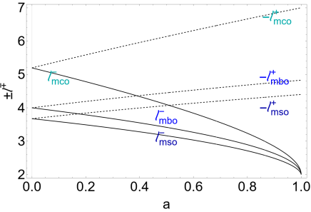
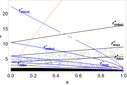
Figure 1: Left panel: Parameter $\ell^{\pm}$ (specific angular momentum) defined in Eq. (8) for co–rotating $(-)$ (solid) and counter–rotating $(+)$ orbits (dashed) as function of the BH dimensionless spin $a$. $mbo$ is for marginally bounded circular orbit, $mco$ is for marginally circular orbit, $mso$ is for marginally stable circular orbit. Right panel: Solid curves are $r_{mco}^{-}<r_{mbo}^{-}<r_{mso}^{-}<r_{(mbo)}^{-}<r_{(mco)}^{-}$ defined in Eqs (14). Blue dotted (gray dotted) region is the range $[r_{mbo}^{-},r_{mso}^{-}]$ ($[r_{mbo}^{+},r_{mso}^{+}]$) for the location of the co–rotating (counter–rotating) disk cusp. Brown solid, dashed and dotted–dashed curves are the inversion radii $r_{{\mbox{\scriptsize{{T}}}}}(\ell_{mso}^{+})>r_{{\mbox{\scriptsize{{T}}}}}(\ell_{mbo}^{+})>r_{{\mbox{\scriptsize{{T}}}}}(\ell_{mco}^{+})$. Pink (yellow) curves are for $\ell^{+}=\ell^{+}_{mso}/100$ ($\ell^{+}=\ell^{+}_{mso}/10$). All quantities are dimensionless.

The inner edge of an accretion disk orbiting the central BH on its equatorial plane, is generally assumed to be in the range $[r_{mbo}^{\pm},r_{mso}^{\pm}]$, for counter–rotating and co–rotating disks respectively, and its precise location depends on the central attractor features and the disks characteristics. This constraint on the accretion disk inner edge is widely adopted (and well grounded) in BH Astrophysics, and in the following analysis we will use this assumption independently of other specific details of the accretion disk models.

However, to make our arguments more precise, we discuss an example of General Relativistic Hydrodynamical (GRHD) toroidal configurations–[62]. These configurations are used to fix up the initial configurations for numerical integration of a broad variety of models. The methodological advantage in the adoption of these models is that the general relativistic thick tori morphological features, related to the equilibrium (quiescent) and accretion phases as cusped closed toroidal surfaces, are determined by the centrifugal and gravitational components of the force balance in the disks, rather then the dissipative effects.

In these models, at the cusp the fluid may be considered pressure-free, and the matter outflows as consequence of an hydro-gravitational instability mechanism, following the violation of mechanical equilibrium in the balance of the gravitational and inertial forces and the pressure gradients in the disks [66]). Showing a remarkably good fitting with the more complex dynamical models, they are largely adopted as initial setup for numerical simulations in several general relativistic magnetohydrodynamic (GRMHD) models, constituting also a comparative model in many numerical analysis of complex situations–[62, 67, 68, 69, 70].

$\mathbf{L_{1}}$	$\mp\ell^{\pm}\equiv[\mp\ell_{mso}^{\pm},\mp\ell_{mbo}^{\pm}[$:	$\textbf{()}_{1}:$ Quiescent (i.e. not cusped) $\mathrm{C}_{1}$ and cusped tori $\mathrm{C}_{\times}$.
	The cusp is $r^{\pm}_{\times}\in]r^{\pm}_{mbo},r^{\pm}_{mso}]$ ($K_{\times}^{\pm}<1$)).
	The torus center is $r^{\pm}_{center}\in]r^{\pm}_{mso},r^{\pm}_{(mbo)}]$.
$\mathbf{L_{2}}$	$\mp\ell^{\pm}\equiv[\mp\ell_{mbo}^{\pm},\mp\ell_{mco}^{\pm}[$:	$\textbf{()}_{2}:$ Quiescent tori $\mathrm{C}_{2}$ and proto-jets.
	The torus cusp is $r_{\times}^{\pm}\in]r_{mco}^{\pm},r_{mbo}^{\pm}]$ (proto-jets $K_{\times}>1$).
	The torus center is $r_{center}^{\pm}\in]r_{(mbo)}^{\pm},r_{(mco)}^{\pm}]$.
$\mathbf{L_{3}}$	$\mp\ell^{\pm}\geq\mp\ell_{mco}^{\pm}$:	$\textbf{()}_{3}:$ Quiescent tori $\mathrm{C}_{3}$.
	The torus center is $r^{\pm}_{center}>r_{(mco)}^{\pm}$.

Table 1: Geometrically thick GRHD tori orbiting Kerr BHs. $\ell$ is the specific fluid angular momentum. $mbo$ is for marginally bounded circular orbit, $mco$ is for marginally circular orbit, $mso$ is for marginally stable circular orbit. $\pm$ is for counter–rotating and co–rotating fluids respectively. Radii $r_{(mbo)}^{\pm}$ and $r_{(mco)}^{\pm}$ are defined in Eq. (14) and, together with the radii of geodesic structure, form the Kerr spacetime extended geodesic structure–Fig. 1. Fluid effective potential $V_{eff}(\ell,a,r)$ defines the function $K(a,r)=V_{eff}(\ell(r,a),a,r)$. Torus cusp $r_{\times}$ is the minimum point of pressure and density in the torus. The torus center $r_{center}$ is the fluid maximum point of pressure and density. Cusped tori have parameter $K=K_{\times}\equiv K(r_{\times})\in]K_{center},1[\subset]K_{mso},1[$, where $K_{center}\equiv K(r_{center})$. Proto-jets are open cusped configurations. Notation $\mathrm{C}^{\pm}$ ($\mathrm{C}_{\times}^{\pm}$) is for quiescent (cusped) tori, $\textbf{()}^{\pm}$ for quiescent or cusped configurations, $r_{outer}$ is the torus outer edge and the notation $\mathcal{Q}(L_{\bullet})$ or $\mathcal{Q}_{\bullet}$ for $\bullet\in\{1,2,3\}$ for configurations $\mathcal{Q}$ with momenta in the range $\mathbf{L_{\bullet}}$.

In Sec. (III.1) we discuss the model in some detail, developing the analytical conditions adopted in the following analysis.

III.1 Thick accretion disk model in the Kerr spacetime

We focus on general relativistic barotropic toroidal configurations which are geometrically thick and optical opaque. The toroids, composed by a one particle-specie perfect fluid, are cooled by advection, and are axially symmetric and stationary. Exploring the case of a one-species particle perfect fluid (simple fluid), each torus is described by the energy momentum tensor

$$T_{\alpha\beta}=(\rho+p)u_{\alpha}u_{\beta}+\ pg_{\alpha\beta},$$ (10)

where $\rho$ and $p$ are the total energy density and pressure, respectively, as measured by an observer moving with the fluid whose four-velocity $u^{\alpha}$ is a timelike flow vector field. (For the symmetries of the problem, we always assume $\partial_{t}\mathbf{Q}=0$ and $\partial_{\phi}\mathbf{Q}=0$, being $\mathbf{Q}$ a generic spacetime tensor.).

From the GRHD equations we find that the fluid dynamics is described by the continuity equation and the Euler equation respectively:

$$u^{\alpha}\nabla_{\alpha}\rho+(p+\rho)\nabla^{\alpha}u_{\alpha}=0\,,\quad(p+\rho)u^{\alpha}\nabla_{\alpha}u^{\gamma}+\ h^{\beta\gamma}\nabla_{\beta}p=0\,,$$ (11)

where the projection tensor $h_{\alpha\beta}=g_{\alpha\beta}+u_{\alpha}u_{\beta}$ and $\nabla_{\alpha}g_{\beta\gamma}=0$. The toroids are centered on the plane $\theta=\pi/2$, and defined by the constraint $u^{r}=0$. (No motion is assumed in the $\theta$ angular direction, which means $u^{\theta}=0$.) We assume moreover a barotropic equation of state $p=p(\rho)$.

The continuity equation in Eq. (11) is identically satisfied as consequence of these conditions and, from the Euler equation (11), one finds

$$\frac{\partial_{\mu}p}{\rho+p}=-{\partial_{\mu}W}+\frac{\Omega\partial_{\mu}\ell}{1-\Omega\ell},\quad\mbox{with}\quad\ell\equiv\frac{L}{E}$$ (12)

$$\mbox{where}\quad W\equiv\ln V_{eff}(\ell),\quad\mbox{and }\quad V_{eff}(\ell)=\sqrt{\frac{g_{\phi t}^{2}-g_{tt}g_{\phi\phi}}{g_{\phi\phi}+2\ell g_{\phi t}+\ell^{2}g_{tt}}},$$

where the function $W$ is Paczynski-Wiita (P-W) potential and $V_{eff}(\ell)$ provides an effective potential for the fluid, assumed here to be characterized by a conserved and constant specific angular momentum $\ell$.

The procedure adopted in the present article borrows from the Boyer theory on the equi–pressure surfaces applied to a thick torus: the Boyer surfaces are given by the surfaces of constant pressure or $\Sigma_{i}=$constant for $i\in(p,\rho,\ell,\Omega)$, where the angular frequency is indeed $\Omega=\Omega(\ell)$ and $\Sigma_{i}=\Sigma_{j}$ for ${i,j}\in(p,\rho,\ell,\Omega)$. (More generally $\Sigma_{\mathbf{Q}}$ is the surface $\mathbf{Q}=$constant for any quantity or set of quantities $\mathbf{Q}$.)

The toroidal surfaces are the equipotential surfaces of the effective potential $V_{eff}(\ell)$, considered as function of $r$, solutions $\ln(V_{eff})=\rm{c}=\rm{constant}$ or $V_{eff}=K=$constant.

Extreme points of the co–rotating toroids

In the first and simplest realization of this model each orbiting configuration is therefore parametrized by a constant fluid specific angular momentum $\ell$ (defined in Eq. (8)), as a torus parameter [62, 31]. The model is therefore regulated by the couple of parameters $\mathbf{p}\equiv(\ell,K)$ which together uniquely identify each equi-pressure (equi-potential) surface.

Therefore, from Eq. (12), it is clear that the maximum and minimum density points (the pressure gradients) in the disk, which are the toroids centers and cusps respectively, are fixed by the gradients of a scalar, the fluid effective potential $V_{eff}$ in Eq. (12), depending on the BH spin $a$, the fluid specific angular momentum $\ell$, and the radial distance from the central attractor (the function is evaluated on the toroid equatorial plane which is also the BH equatorial plane).

Note, in general the curve $\ell^{\pm}_{\sigma}=$constant, defined by $\ell^{\pm}_{\sigma}:\partial_{y}V_{eff}^{2}=0$, where there is $\{z=r\cos\theta,y=r\sin\theta\sin\phi,x=r\sin\theta\cos\phi\}$, provides the pressure (and density) extreme points on the equatorial plane and counter–rotating and co–rotating tori geometrical extremes respectively.

The extremes of the pressure are therefore regulated by the angular momentum distributions, as there is $\ell=\ell(r,\theta;a):\partial_{r}V_{eff}=0$ on the equatorial plane $\theta=\pi/2$. Explicitly the specific angular momentum for the co–rotating and counter–rotating toroids are

$$\ell^{\mp}=\frac{-a^{3}\pm\sqrt{r^{3}\left(a^{2}+(r-2)r\right)^{2}}+ar(4-3r)}{(r-2)^{2}r-a^{2}}$$ (13)

respectively. (Note $\ell^{\mp}=\ell_{\sigma}^{\mp}$ for $\sigma=1$)

The $K$ parameter and the toroids

There are three sets of configurations defined by the range of values of the momentum $\ell$, and $K=$constant as described in Table 1.

The flows considered in this analysis are defined by the parameter $\ell$ for “accretion driven” and “proto-jets driven” flows, having $\mp\ell^{\pm}\in[\mp\ell_{mso}^{\pm},\mp\ell_{mbo}^{\pm}]$ related to tori or, having $\mp\ell^{\pm}\in[\mp\ell_{mbo}^{\pm},\mp\ell_{mco}^{\pm}]$ as proto-jet configurations, which are open toroidal surfaces made by funnels of matter, along the BH symmetry axis having a cusp on the equatorial plane in the range $r_{J}^{\pm}\in[r_{mbo}^{\pm},r_{mco}^{\pm}]$–[57].

The tori and proto–jets cusps, corresponding to the minimum points of the hydrodynamic pressure, can be found from $V_{eff}$ of Eq. (12) , as the maximum points of the effective potential function with $K<1$ or $K>1$ respectively–see also Tabel 1.

The location of the configurations centers, $r_{center}^{\pm}$ (which can be easy found as minimum points of the effective potential $V_{eff}$ in Eq. (12) with $\ell=$constant), is constrained by the fluids specific angular momentum $\ell$, according to the radii $r_{(mbo)}^{\pm}$ and $r_{(mco)}^{\pm}$, defined by the relations:

$$r_{\mathrm{(mbo)}}^{\pm}:\;\ell^{\pm}(r_{\mathrm{mbo}}^{\pm})=\ell^{\pm}(r_{\mathrm{(mbo)}}^{\pm})\equiv\mathbf{\ell_{\mathrm{mbo}}^{\pm}},\quad r_{(mco)}^{\pm}:\ell^{\pm}(r_{mco}^{\pm})=\ell^{\pm}(r_{(mco)}^{\pm})\equiv\ell_{mco}^{\pm}\quad\mbox{where}$$

$$r_{mco}^{\pm}<r_{\mathrm{mbo}}^{\pm}<r_{\mathrm{mso}}^{\pm}<r_{\mathrm{(mbo)}}^{\pm}<r_{(mco)}^{\pm}$$ (14)

as described in Table 1. Radii $(r_{\mathrm{(mbo)}}^{\pm},r_{(mco)}^{\pm})$ form, with the geodesic radii, the extended geodesic structure of the Kerr spacetime–Fig. 1.

In the following it will be useful to specify the case for the co–rotating toroids. The cusps and center of co–rotating torus, $r_{\times}^{-}<r_{mso}^{-}<r_{center}^{-}$ or proto-jets $r_{J}^{-}<r_{mso}^{-}<r_{center}^{-}$ can be found in terms of the parameter $\ell$, solving the equation $\ell^{-}(r)=\ell$, and there is

$$r_{center}^{-}\equiv\frac{\xi+\Xi}{12}\quad\mbox{and}\quad r_{\times}^{-}\equiv\frac{\xi-\Xi}{12},\quad\mbox{where}$$ (15)

$$\xi\equiv\sqrt{3}\sqrt{B_{5}}+3\ell^{2},\quad\Xi\equiv\sqrt{6}\sqrt{\frac{3\sqrt{3}\left(\ell^{6}-8B\ell^{2}+32B_{1}\right)}{\sqrt{B_{5}}}-16B-\frac{8\sqrt[3]{2}B_{0}}{\sqrt[3]{B_{4}}}-2^{2/3}\sqrt[3]{B_{4}}+3\ell^{4}},$$

with

$$B\equiv a^{2}-3a\ell+2\ell^{2},\quad B_{0}\equiv\left(2a^{2}-3a\ell+\ell^{2}\right)^{2},$$ (16)

$$B_{1}\equiv a^{2}-2a\ell+\ell^{2};$$

$$B_{2}\equiv-72BB_{1}\left(2a^{2}+\ell^{2}\right)+27B_{1}\left(a^{2}\ell^{4}+16B_{1}\right)+16B^{3},\quad B_{3}\equiv B_{2}^{2}-4(4B_{0})^{3},\quad B_{4}\equiv B_{2}+\sqrt{B_{3}},$$

$$B_{5}\equiv-16B+\frac{16\sqrt[3]{2}B_{0}}{\sqrt[3]{B_{4}}}+2\ 2^{2/3}\sqrt[3]{B_{4}}+3\ell^{4}.$$

The closed surfaces cross in general the equatorial plane in three points, including the inner and outer edges of the closed configurations. The equi-potential surfaces identify therefore the inner and outer edges of the quiescent (not cusped) tori, as $r_{inner}<r_{center}<r_{outer}$.

It will be convenient to use the notation $\mathrm{C}^{\pm}$ ($\mathrm{C}_{\times}^{\pm}$) for quiescent (cusped) tori, $\textbf{()}^{\pm}$ for quiescent or cusped configurations, $r_{outer}$ is the torus outer edge, $r_{\times}$ for the torus cusp, and the notation $\mathcal{Q}(\mathbf{L_{\bullet}})$ or $\mathcal{Q}_{\bullet}$ for $\bullet\in\{1,2,3\}$ for quantity $\mathcal{Q}$ with momenta in the range $\mathbf{L_{\bullet}}$, according to Table 1. Symbols $\lessgtr$ for two tori refer to the relative position of the tori, for example, we use short notation $\mathrm{C}_{\times}^{-}<\mathrm{C}_{\times}^{+}$ for $r_{\times}^{-}<r_{center}^{-}<r_{outer}^{-}<r_{\times}^{+}<r_{center}^{+}<r_{outer}^{+}$. Since the toroidal configurations can be corotating $\ell a>0$ or counterrotating $\ell a<0$, with respect to the black hole $a>0$, then assuming several toroidal configurations, say the couple $(\mathrm{C}_{a},\mathrm{C}_{b})$, with proper angular momentum $(\ell_{a},\ell_{b})$ orbiting in the equatorial plane of a given Kerr BH, they can be $\ell$corotating disks, defined by the condition $\ell_{a}\ell_{b}>0$, or $\ell$counterrotating disks by the relations $\ell_{a}\ell_{b}<0$, where the two $\ell$corotating tori can be both corotating $\ell a>0$ or counterrotating $\ell a<0$ with respect to the central attractor.

IV Inversion surfaces

Inversion points are defined by the condition $u^{\phi}=0$ for particles and photons– [1]. It the context of the inversion points it is convenient to use the notation $u$counter–rotating ($u$co–rotating) for matter and photons with $u^{\phi}<0$ ($u^{\phi}>0$), along side with counter–rotating for $\ell<0$ (co–rotating for $\ell>0$). Located out of the (outer) ergoregion, and totally embedding the central BH–see Fig. 2– they are defined for counter–rotating trajectories ($\ell<0$), and they can be interpreted as an effect of the Kerr spacetime frame–dragging acting on the $u$counter–rotating particles (and photons) accreting into the central BH–Figs 3,4.

The inversion surfaces are defined by a general, necessary but not sufficient, condition, $u^{\phi}=0$, on materials (including photons) ingoing towards the BH, or outgoing or moving along the BH spinning axis. However, an initially $u$counter–rotating flow of matter and photons accreting into the central BH will have an inversion point at the inversion surface, as defined by its (conserved) specific angular momentum $\ell<0$.

At the inversion point there is the inversion radius $r=r_{\mbox{\scriptsize{{T}}}}$ on a plane $\sigma=\sigma_{\mbox{\scriptsize{{T}}}}$:

$$r_{{\mbox{\scriptsize{{T}}}}}\equiv\sqrt{a^{2}\left(\sigma_{\mbox{\scriptsize{{T}}}}+\frac{\sigma_{\mbox{\scriptsize{{T}}}}^{2}}{\ell^{2}}-1\right)-\frac{2a\sigma_{\mbox{\scriptsize{{T}}}}}{\ell}+1}-\frac{a\sigma_{\mbox{\scriptsize{{T}}}}}{\ell}+1\quad\mbox{where}\quad\lim\limits_{\ell\rightarrow-\infty}r_{{\mbox{\scriptsize{{T}}}}}=r_{\epsilon}^{+},\quad\lim\limits_{a\rightarrow 0}r_{{\mbox{\scriptsize{{T}}}}}=\lim\limits_{\sigma\rightarrow 0}r_{{\mbox{\scriptsize{{T}}}}}=r_{+},$$ (17)

(see Figs 5,2).

In the following, we use the notation $\mathrm{Q}_{\mbox{\scriptsize{{T}}}}$ for any quantity $\mathrm{Q}$ considered at the inversion point, and therefore on the inversion point there is $\ell=\ell_{\mbox{\scriptsize{{T}}}}$, $\sigma=\sigma_{\mbox{\scriptsize{{T}}}}$, $\dot{t}=\dot{t}_{\mbox{\scriptsize{{T}}}}$ and

$$\ell_{\mbox{\scriptsize{{T}}}}\equiv\left.-\frac{g_{t\phi}}{g_{tt}}\right|_{\mbox{\scriptsize{{T}}}},\quad\mathcal{E}_{\mbox{\scriptsize{{T}}}}=-g_{tt}({\mbox{\scriptsize{{T}}}})\dot{t}_{\mbox{\scriptsize{{T}}}}=\frac{a\sigma_{\mbox{\scriptsize{{T}}}}\dot{t}_{\mbox{\scriptsize{{T}}}}}{a\sigma_{\mbox{\scriptsize{{T}}}}-\ell},\quad\mathcal{L}_{\mbox{\scriptsize{{T}}}}=g_{t\phi}({\mbox{\scriptsize{{T}}}})\dot{t}_{\mbox{\scriptsize{{T}}}}=\frac{a\sigma_{\mbox{\scriptsize{{T}}}}\dot{t}_{\mbox{\scriptsize{{T}}}}\ell}{a\sigma_{\mbox{\scriptsize{{T}}}}-\ell}.$$ (18)

At fixed $\ell<0$, radius $r_{\mbox{\scriptsize{{T}}}}(\sigma_{\mbox{\scriptsize{{T}}}})$ defines the inversion surface $\mathrm{S}_{\mbox{\scriptsize{{T}}}}$ of momentum $\ell$ and a region, inversion sphere, embedding the central attractor, upper bounded by the inversion surface and bottom bounded by the BH outer ergosurface. The photon or particle inversion point $(r_{\mbox{\scriptsize{{T}}}},\theta_{\mbox{\scriptsize{{T}}}},\phi_{\mbox{\scriptsize{{T}}}})$ on the inversion surface can be determined by the set of equations (5) which also relates $(r_{\mbox{\scriptsize{{T}}}},\sigma_{\mbox{\scriptsize{{T}}}})$ to the initial values $(r_{0},\sigma_{0})$, depending on the single particle trajectory.

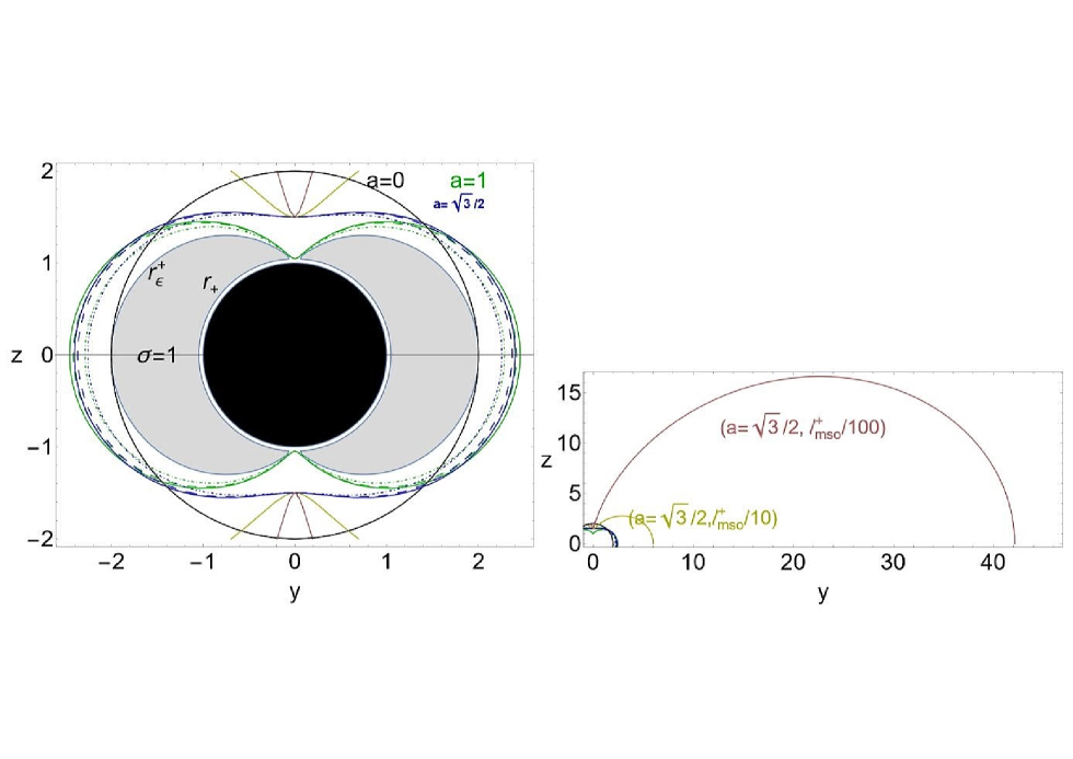
Figure 2: Inversion surfaces in the $z-y$ plane, where $r=\sqrt{y^{2}+z^{2}}$ and $\theta=\arccos({z}/r)$. The counter–rotating flows inversion points $r_{{\mbox{\scriptsize{{T}}}}}$ are evaluated at fluid specific angular momenta $\ell_{mso}^{+}$ (plain) and $\ell_{mbo}^{+}$ (dashed), $\ell_{mco}^{+}$ (dotted-dashed). (There is $\mathrm{Q}_{\bullet}$ for any quantity evaluated at $r_{\bullet}$, and $mbo$ is for marginally bound circular orbit, $mco$ is for marginally circular orbit, $mso$ is for marginally stable circular orbit.). All quantities are dimensionless. Left panel: green curves represent the case for BH dimensionless spin $a=1$ (extreme Kerr spacetime), black curve is $a=0$ (Schwarzschild spacetime), blue curve is for $a=\sqrt{3}/2$. Shaded gray region is the outer ergoregion $]r_{+},r_{\epsilon}^{+}]$, for the BH with spin $a=1$, black region is the central BH with spin $a=1$. Right panel: is a different view of the left panel for the spin and momenta signed on the panel.

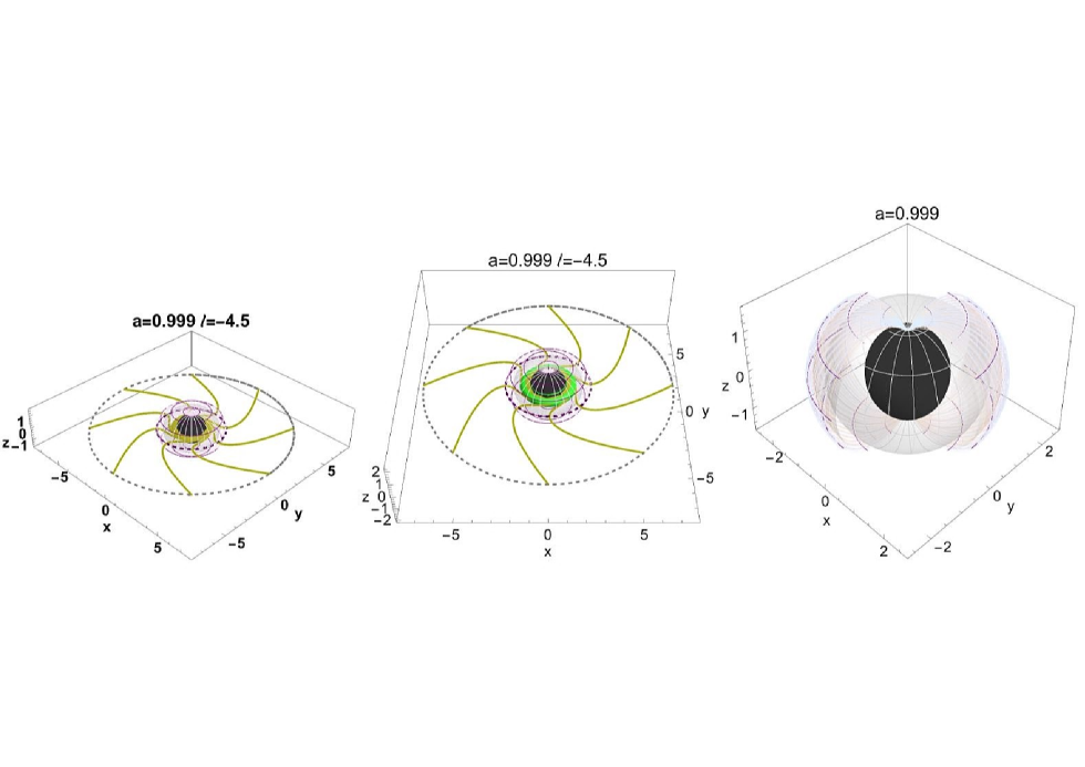
Figure 3: Left panel: tori driven counter–rotating photons inversion points in the BH spacetimes with dimensionless spin $a=0.999$. The impact parameter (specific angular momentum) is $\ell=-4.5$, where there is $\{z=r\cos\theta,y=r\sin\theta\sin\phi,x=r\sin\theta\cos\phi\}$ in dimensionless units. The parameter $\ell$ is defined in Eq. (8). The panel shows a view of the counter–rotating flow stream from a torus (equi-potential surface with $\ell=-4.5$) inner edge (cusp-dashed gray curve) to the central BH (black region $r<r_{+}$, radius $r_{+}$ is the outer horizon). Flow inversion point $r_{{\mbox{\scriptsize{{T}}}}}$ is plotted as the deep-purple curve. Radius $r_{{\mbox{\scriptsize{{T}}}}}$ lies in the inversion corona defined by the range $(r_{\mbox{\scriptsize{{T}}}}(\ell_{mso}^{+})-r_{\mbox{\scriptsize{{T}}}}(\ell_{mbo}^{+}))$. (There is $\mathrm{Q}_{\bullet}$ for any quantity evaluated at $r_{\bullet}$, and $mbo$ is for marginally bounded circular orbit, $mso$ is for marginally stable circular orbit.). Gray region is the outer ergosurface, light-purple shaded region is the region $r<r_{\mbox{\scriptsize{{T}}}}(\sigma_{\mbox{\scriptsize{{T}}}})$. Right panel: Sections of the inversion spheres with radius $r_{\mbox{\scriptsize{{T}}}}(\ell_{mso}^{+})>r_{\mbox{\scriptsize{{T}}}}(\ell_{mbo}^{+})>r_{\mbox{\scriptsize{{T}}}}(\ell_{mco}^{+})$ for $a=0.999$ (blue, purple and orange surfaces), gray region is the outer ergoregion, black region is the central BH. All quantities are dimensionless.

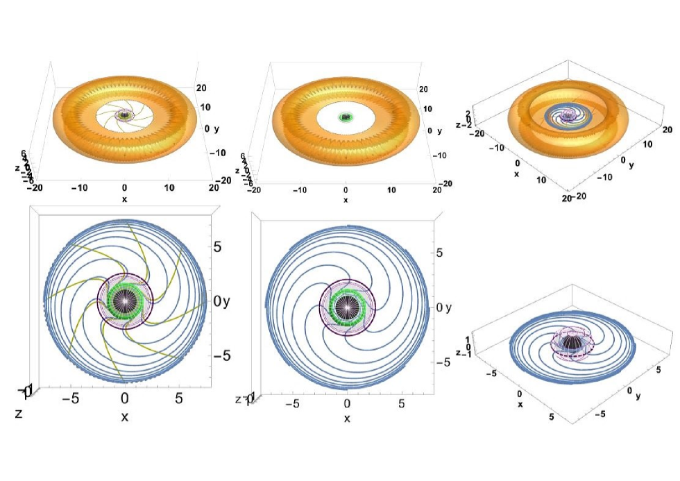
Figure 4: Tori driven counter–rotating photons inversion points in the BH spacetimes with dimensionless spin $a=0.999$. The impact parameter (specific angular momentum) is $\ell=-4.5$, where there is $\{z=r\cos\theta,y=r\sin\theta\sin\phi,x=r\sin\theta\cos\phi\}$ in dimensionless units. The panels show a view of the counter–rotating flow stream from a torus inner edge (cusp-dashed gray curve) to the central BH (black region $r<r_{+}$, radius $r_{+}$ is the outer horizon). The torus is a cusped equi-pressure surface defined by the parameter $\ell=-4.5$,Orange outer (inner) surface is the counter–rotating (co–rotating) torus. Yellow (blue) curves are photons (test particles) trajectories. (See caption Fig. 3 for further details.)

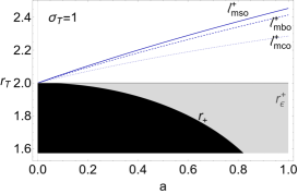
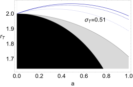
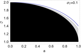
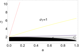
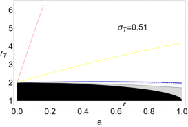
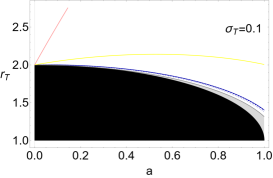
Figure 5: Inversion radius $r_{\mbox{\scriptsize{{T}}}}$ (where $u^{\phi}$=0) as function of the BH dimensionless spin $a$ for different angles $\sigma\equiv\sin^{2}\theta$ signed on the panel and different $\ell^{+}$ (specific angular momentum) defined in Eq. (8) for counter–rotating $(+)$ orbits. There is $\mathrm{Q}_{\bullet}$ for any quantity evaluated at $r_{\bullet}$, where $mbo$ is for marginally bound circular orbit, $mco$ is for marginally circular orbit, $mso$ is for marginally stable circular orbit. Pink (yellow) curves are for $\ell^{+}=\ell^{+}_{mso}/100$ ($\ell^{+}=\ell^{+}_{mso}/10$). All quantities are dimensionless. Black region is the central BH, $r_{+}$ is the outer horizon, gray region is the outer ergoregion, radius $r_{\epsilon}^{+}$ is the outer ergosurface.

Hence, the region defined by the radii $r_{\mbox{\scriptsize{{T}}}}(\ell^{+}_{\bullet})$ and $r_{\epsilon}^{+}(a,\sigma)$ contains all the inversion surfaces $\mathrm{S}_{\mbox{\scriptsize{{T}}}}(\ell^{+}_{\star})$ with $\ell^{+}_{\star}\leq\ell^{+}_{\bullet}$. Therefore we can define an inversion corona, as the shell bounded by the inversion surfaces of radius $r_{\mbox{\scriptsize{{T}}}}(\sigma_{\mbox{\scriptsize{{T}}}})$ in the range $[r_{\mbox{\scriptsize{{T}}}}(\ell_{mbo}^{+})],r_{\mbox{\scriptsize{{T}}}}(\ell_{mso}^{+})]$, for accretion driven counter–rotating flows, and $[r_{\mbox{\scriptsize{{T}}}}(\ell_{mbo}^{+})],r_{\mbox{\scriptsize{{T}}}}(\ell_{mco}^{+})]$ for proto-jets driven counter–rotating flows, where there is $r_{{\mbox{\scriptsize{{T}}}}}(\ell_{mso}^{+})>r_{{\mbox{\scriptsize{{T}}}}}(\ell_{mbo}^{+})>r_{{\mbox{\scriptsize{{T}}}}}(\ell_{mco}^{+})$–Fig. 5. Surface $\mathrm{S}_{\mbox{\scriptsize{{T}}}}$, as well as the radius $r_{\mbox{\scriptsize{{T}}}}$, are uniquely defined by the momentum $\ell^{+}_{\mbox{\scriptsize{{T}}}}$, and we can use, with no ambiguity, notation $r_{{\mbox{\scriptsize{{T}}}}}(\ell_{\mbox{\scriptsize{{T}}}}^{+})$ for the surface $\mathrm{S}_{\mbox{\scriptsize{{T}}}}$ with momentum $\ell_{\mbox{\scriptsize{{T}}}}^{+}$. In the following with radius $r_{{\mbox{\scriptsize{{T}}}}}(\mathbf{L_{\bullet}^{+}})$ we also indicate any inversion surface $\mathrm{S}_{\mbox{\scriptsize{{T}}}}$ (and inversion radius $r_{\mbox{\scriptsize{{T}}}}$) defined by a momentum in the range $\mathbf{L_{\bullet}^{+}}$, and we equally indicate the entire set of inversion surfaces with momentum in $\mathbf{L_{\bullet}^{+}}$. Hence, according to this notation, there is $r_{{\mbox{\scriptsize{{T}}}}}(\mathbf{L_{3}^{+}})<r_{{\mbox{\scriptsize{{T}}}}}(\mathbf{L_{2}^{+}})<r_{{\mbox{\scriptsize{{T}}}}}(\mathbf{L_{1}^{+}})$. A toroid $\textbf{()}_{\bullet}$ with momentum in the range $\mathbf{L_{\bullet}}$, is contained in (or embedded in, or internal to) an inversion surface $r_{\mbox{\scriptsize{{T}}}}^{+}$ if $\textbf{()}_{\bullet}<r_{\mbox{\scriptsize{{T}}}}^{+}$, and it is external to an inversion surface if $\textbf{()}_{\bullet}>r_{\mbox{\scriptsize{{T}}}}^{+}$.

A configuration, (entirely) contained in such inversion surface, is therefore shielded from impact with $u$counter–rotating material or photons accreting into the central BH.

The distance, $r_{\mbox{\scriptsize{{T}}}}(\ell_{mso}^{+})-r_{\mbox{\scriptsize{{T}}}}(\ell_{mbo}^{+})$, increases not monotonically with the BH spin–mass ratio and with the plane $\sigma$–see Fig. 5 and Figs 4,2–[1]. Radii ($r_{\mbox{\scriptsize{{T}}}}(\ell_{mco}^{+}),r_{\mbox{\scriptsize{{T}}}}(\ell_{mbo}^{+}),r_{\mbox{\scriptsize{{T}}}}(\ell_{mso}^{+})$) vary little with the BH spin and plane $\sigma$. Therefore, the flow in this region is actually located in a restricted orbital range $(r_{{\mbox{\scriptsize{{T}}}}},\sigma_{{\mbox{\scriptsize{{T}}}}})$, localized in the orbital cocoon surrounding the central attractor outer ergosurface) (see for example Figs 2–left panel).

All the co–rotating toroids orbiting in the BH outer ergoregion (totally contained in the ergoregion) are embedded in all the inversion surfaces and will not be in contact with the $u$counter–rotating flows. In Fig. 6–left panel is an example of inter–disks inversion surface in the system $\mathrm{C}^{-}<\mathrm{S}_{\mbox{\scriptsize{{T}}}}(\ell^{+})<\mathrm{C}^{+}_{\times}$, where the inner co–rotating torus orbits in the BH ergoregion. In the next section we will explore the case of a co–rotating toroid and an inversion surface with momenta $\ell^{+}<\ell_{mso}^{+}$, focusing on the inter–surfaces inversion surfaces, i.e. the case $\textbf{()}^{-}<\mathrm{S}_{\mbox{\scriptsize{{T}}}}<\textbf{()}^{+}$, the situation in which the inner surface is co–rotating, and the counter–rotating fluids originate from (are related to) an outer counter–rotating accreting disk. In particular we shall examine the case of a quiescent or cusped disks. The case of inversion surfaces in relation to a double orbiting configurations places additional limits on the BH spin when considered in relation to the presence of an inner co–rotating surface. However, we also discuss the case where one or two orbiting structures are proto–jets (inter proto-jets inversions surfaces).

V Inversion surfaces and inner co–rotating accretion disks

In this section we focus on the co–rotating toroids orbiting a central Kerr BH in relation to the spacetime inversion surfaces. The analysis ultimately provides the conditions when a co–rotating disk or proto–jet can collide with and be replenished by $u$counter–rotating (counter–rotating) matter and photons accreting into the central BH or, viceversa when, counter–rotating matter and photons impacting on the surface will be $u$co–rotating. This condition is strictly constrained by the flow parameters $\ell^{\pm}$, for the inversion surface, the orbiting toroids (disks or proto–jets), and the BH spin $a$. In particular, depending on the parameters $\ell$ and $K$ , disks and proto-jets can be: 1. embedded in an inversion surface ($\textbf{()}^{-}<\mathrm{S}_{\mbox{\scriptsize{{T}}}}$); 2. located out of the inversion surface ($\mathrm{S}_{\mbox{\scriptsize{{T}}}}<\textbf{()}^{-}$); or 3. crossing the inversion surfaces in particular points (for example the center, the geometrical maximum), being partially contained in the inversion surface.

These three scenarios will be considered as framework for the analysis of Sec. (V.2), where we will investigate the inversion surfaces crossing the inner co–rotating toroids. Some preliminary aspects are examined in Sec. (V.1), where characteristics of the Kerr spacetimes inversions surfaces will be discussed in relation to the toroids orbiting the BH, distinguishing BH classes by the properties of the inversion surfaces in relation to co–rotating toroids.

V.1 BHs and inter–disks inversion surfaces

As there is $r_{\mbox{\scriptsize{{T}}}}(\ell_{mso}^{+})<r_{mco}^{+}$–see Figs 1,7,8– the cusped and quiescent counter–rotating tori and proto–jets are always external to inversion surfaces (i.e. there is $r_{\mbox{\scriptsize{{T}}}}(\ell^{+})<\textbf{()}^{+}$). Hence, we concentrate on the inner co–rotating toroids in a double orbiting system (that is the case $\textbf{()}^{-}<\textbf{()}^{+}$).

Our analysis is limited to the counter–rotating flows and the inversion surfaces with momenta in the range $-\ell^{+}>-\ell^{+}_{mso}$. However, for small momentum in magnitude, the inversion surfaces can always cross the counter–rotating geodesic structure radii (and therefore can intersect counter–rotating toroids or even be external to a counter–rotating toroid)–Fig. 1. This case occurs for inversion surfaces momenta $\ell^{+}\in[\ell_{G}^{+}(r_{mco}^{+}),0[$, where

$$\ell_{G}^{+}(r)\equiv\frac{2a}{2-r},\quad\mbox{with}\quad\ell_{G}^{+}(r):r=\left.r_{\mbox{\scriptsize{{T}}}}^{+}\right|_{\sigma=1}$$ (19)

where $\ell_{G}^{+}(r_{mco}^{+})>\ell_{mso}^{+}$ – (see Fig. 9 and Figs 1,5,2 (pink and yellow curves)).

On the other hand, part of our considerations focuses on the inversion surfaces properties on the equatorial plane, discussing the location of the inversion radius $r_{{\mbox{\scriptsize{{T}}}}}(\ell^{+})$ in relation to the (co–rotating) geodesic structure. However, conditions defined on the equatorial plane may not be satisfied at $\sigma<1$, for example this could be the case for a partially contained toroids, crossing an inversion surface on planes other than the equatorial. The off–equatorial properties are determined by the characteristics of the specific accretion disk model and regulated by the inversion surfaces characteristics, which are fixed exclusively by the background geometry. (The inversion surfaces “maximum radial elongation” occurs on the equatorial plane, the maximum radial distance from the central BH is $r\approx 2.45455$ –Fig. 2.) We address the off–equatorial case in details in Sec. (V.2.5).

The inversion surfaces radii $r_{{\mbox{\scriptsize{{T}}}}}$ are shown in Fig. 7 and Fig. 8 in relation to the co–rotating geodesic structure for different BH spins. We distinguish sixteen BHs classes, defined by the spins in Table 2 and shown in Figs 6,7,8. The boundary spins are defined by the intersection between the inversion surfaces radii $r_{\mbox{\scriptsize{{T}}}}(\ell^{+}_{\bullet})$ for $\ell^{+}_{\bullet}\in\{\ell^{+}_{mso},\ell^{+}_{mbo},\ell^{+}_{mco}\}$ with the co–rotating extended geodesic structure –see Figs 7,8.

Therefore, we introduce the notation

$$a_{(\hat{\bullet},\hat{\star})}:r_{\mbox{\scriptsize{{T}}}}(\ell_{\bullet}^{+})=r_{\star}^{-}\quad\mbox{and}\quad a_{((\hat{\bullet},\hat{\star}))}:r_{\mbox{\scriptsize{{T}}}}(\ell_{\bullet}^{+})=r_{(\star)}^{-},\quad\mbox{where}\quad\{(\hat{\bullet},{\bullet}),(\hat{\star},{\star})\}\in\{(s,mso),(b,mbo),(c,mco)\},$$ (20)

and we can define the spins $a_{(\bullet,s)}=\{a_{(s,s)},a_{(b,s)},a_{(c,s)}\}$, where the following relations hold:

$$a_{(s,\star)}<a_{(b,\star)}<a_{(c,\star)}\quad\mbox{and}\quad a_{((b,\star))}<a_{((c,\star))}\quad\mbox{for}\quad\star\in\{s,b,c\}.$$ (21)

$a_{(c,s)}=0.908096:r_{\mbox{\scriptsize{{T}}}}(\ell_{mco}^{+})=r_{mso}^{-}$	$a_{(c,b)}=0.75673:r_{\mbox{\scriptsize{{T}}}}(\ell_{mco}^{+})=r_{mbo}^{-}$	$a_{(c,c)}=0.599433:r_{\mbox{\scriptsize{{T}}}}(\ell_{mco}^{+})=r_{mco}^{-}$
$a_{(b,s)}=0.891799:r_{\mbox{\scriptsize{{T}}}}(\ell_{mbo}^{+})=r_{mso}^{-}$	$a_{(b,b)}=0.728163:r_{\mbox{\scriptsize{{T}}}}(\ell_{mbo}^{+})=r_{mbo}^{-}$	$a_{(b,c)}=0.5625:r_{\mbox{\scriptsize{{T}}}}(\ell_{mbo}^{+})=r_{mco}^{-}$,
$a_{(s,s)}=0.886532:r_{\mbox{\scriptsize{{T}}}}(\ell_{mso}^{+})=r_{mso}^{-}$	$a_{(s,b)}=0.719111:r_{\mbox{\scriptsize{{T}}}}(\ell_{mso}^{+})=r_{mbo}^{-}$	$a_{(s,c)}=0.550895:r_{\mbox{\scriptsize{{T}}}}(\ell_{mso}^{+})=r_{mco}^{-}$
$a_{((c,c))}=0.989421:r_{\mbox{\scriptsize{{T}}}}(\ell_{mco}^{+})=r_{(mco)}^{-}$	$a_{((c,b))}=0.986806:r_{\mbox{\scriptsize{{T}}}}(\ell_{mbo}^{+})=r_{(mco)}^{-}$	$a_{((c,s))}=0.985935:r_{\mbox{\scriptsize{{T}}}}(\ell_{mso}^{+})=r_{(mco)}^{-}$
$a_{((b,c))}=0.98041:r_{\mbox{\scriptsize{{T}}}}(\ell_{mco}^{+})=r_{(mbo)}^{-}$	$a_{((b,b))}=0.975354:r_{\mbox{\scriptsize{{T}}}}(\ell_{mbo}^{+})=r_{(mbo)}^{-}$	$a_{((b,s))}=0.973659:r_{\mbox{\scriptsize{{T}}}}(\ell_{mso}^{+})=r_{(mbo)}^{-}$

Table 2: Spins of Eqs (20) shown in Figs 6,7,8. $\ell^{\pm}$ is the specific fluid angular momentum for counter–rotating and co–rotating fluids respectively. $mbo$ is for marginally bounded circular orbit, $mco$ is for marginally circular orbit, $mso$ is for marginally stable circular orbit. Radii $r_{(mbo)}^{\pm}$ and $r_{(mco)}^{\pm}$ are defined in Eq. (14). $r_{\mbox{\scriptsize{{T}}}}$ is the inversion radius.

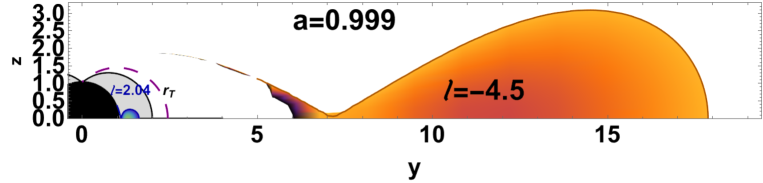
Figure 6: Black region is the central BH with dimensionless spin $a=0.999$. Gray region is the outer ergoregion. Orange (blue) surface, is outer counter–rotating (inner co–rotating) torus (equi-potential surface with fixed specific angular momentum parameter). $\ell$, signed on each toroid, is the fluid specific angular momentum. Dashed curve is the inversion surface $r_{\mbox{\scriptsize{{T}}}}$ at fixed torus counter–rotating angular momentum $\ell^{+}$. There is $r=\sqrt{y^{2}+z^{2}}$ and $\theta=\arccos({z}/r)$. (All quantities are dimensionless.)

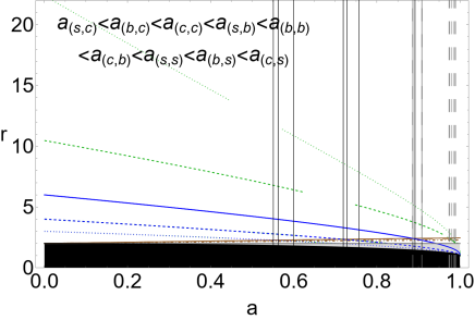
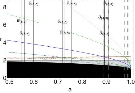
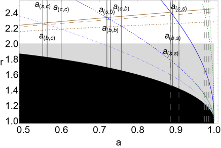
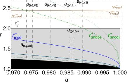
Figure 7: Brown lines are the inversion radii $r_{{\mbox{\scriptsize{{T}}}}}(\ell_{mso}^{+})>r_{{\mbox{\scriptsize{{T}}}}}(\ell_{mbo}^{+})>r_{{\mbox{\scriptsize{{T}}}}}(\ell_{mco}^{+})$, where $\ell^{\pm}$ are the counter–rotating and co–rotating specific angular momentum respectively. Black region is the central BH with dimensionless spin $a$. Gray region is the outer ergoregion on the equatorial plane. (Radius $r_{\epsilon}^{+}$ is the outer ergosurface.) Vertical lines are spins defined in Table 2 (see upper left panel for the vertical solid lines). Upper right and bottom right and left panels are close–up view of the upper left panel. Blue dotted, blue dashed, blue solid and green dashed, green dotted are the radii $r_{mco}^{-}<r_{mbo}^{-}<r_{mso}^{-}<r_{(mbo)}^{-}<r_{(mco)}^{-}$ defined in Eqs (14). $mbo$ is for marginally bound circular orbit, $mco$ is for marginally circular orbit, $mso$ is for marginally stable circular orbit. All quantities are dimensionless.

.

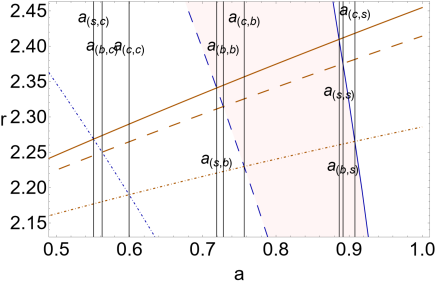
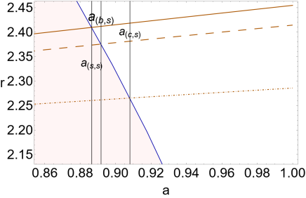
Figure 8: Brown solid, dashed and dotted–dashed curves are the inversion radii $r_{{\mbox{\scriptsize{{T}}}}}(\ell_{mso}^{+})>r_{{\mbox{\scriptsize{{T}}}}}(\ell_{mbo}^{+})>r_{{\mbox{\scriptsize{{T}}}}}(\ell_{mco}^{+})$ respectively, where $\ell^{\pm}$ are the counter–rotating and co–rotating specific angular momentum respectively. Vertical lines are the spins defined in Table 2-(-see for further details also caption of Fig. 7 ($mbo$ is for marginally bound circular orbit, $mco$ is for marginally circular orbit, $mso$ is for marginally stable circular orbit. Pink range is the range $[r_{mbo}^{-},r_{mso}^{-}]$ for the location of the co–rotating disk cusp. Blue dotted-dashed, dashed and solid lines are $r_{mco}^{-}<r_{mbo}^{-}<r_{mso}^{-}$. Right panel is a close–up view of the left panel. All quantities are dimensionless.

.

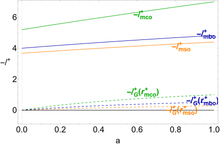
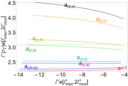
Figure 9: Left panel: Specific angular momentum $\ell_{G}^{+}$ defined in Eq. (19). $a$ is the BH dimensionless spin. $\ell^{\pm}$ are the counter–rotating and co–rotating specific angular momentum respectively. $mbo$ is for marginally bound circular orbit, $mco$ is for marginally circular orbit, $mso$ is for marginally stable circular orbit. Right panel: momentum $\ell^{-}$ is evaluated on the inversion radii $r_{\mbox{\scriptsize{{T}}}}(\ell^{+})$ versus $\ell^{+}$ for different spins defined in Table 2 signed on the panel. The panel shows the momenta $\ell^{\pm}$ of the inversion surface and the inner co–rotating torus, where the inversion surface, with momenta $\ell^{+}$, crosses the co–rotating surface center or cusp at momenta $\ell^{-}$. All quantities are dimensionless.

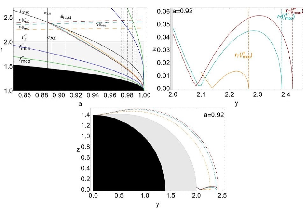
Figure 10: Inversion surfaces crossing the co–rotating accretion disks outer edge. Black region is the central BH, with dimensionless spin $a$. There is $r=\sqrt{y^{2}+z^{2}}$ and $\theta=\arccos({z}/r)$. Gray region is the outer ergoregion ($r_{\epsilon}^{+}$ the outer ergosurface). Dashed lines are the inversion surfaces $r_{\mbox{\scriptsize{{T}}}}$ at fixed counter–rotating angular momentum $\ell^{+}$. Spins signed on the panels are defined in Table 2. All quantities are dimensionless. There is $\mathrm{Q}_{\bullet}$ for any quantity evaluated at $r_{\bullet}$, where $mbo$ (blue curve) is for marginally bound circular orbit, $mco$ (green) is for marginally circular orbit, $mso$ (black curve) is for marginally stable circular orbit. In the upper left panel the outer radii solutions $\ell_{mco}^{-}=\ell^{-}(r)$ (green curve) and $\ell_{mbo}^{-}=\ell^{-}(r)$ (blue curve) are also shown on the BH equatorial plane–(see Eqs (14)). $\ell^{-}$ is the angular momentum for co–rotating fluids. Dotted vertical lines are spins in Fig. 7. Red, cyan and orange solid curves are the inner edges (cusps) correspondent to the solutions of $r_{outer}^{-}=r_{\mbox{\scriptsize{{T}}}}(\ell_{*}^{+})$, where $r_{outer}^{-}$ is the outer edge of a co–rotating cusped torus and $\ell_{*}^{+}\in\{\ell_{mco}^{+},\ell_{mbo}^{+},\ell_{mso}^{+}\}$ (orange, cyan and red curves respectively). Upper right panel and bottom panel show the relative co–rotating tori (dashed curves are the inversion surfaces) found as equi–potential surfaces from $V_{eff}$ of Eq. (12) with constant $\ell_{*}^{+}\in\{\ell_{mco}^{+},\ell_{mbo}^{+},\ell_{mso}^{+}\}$ respectively. Upper right panel is a close–up view of the bottom panel.

.

The spacetimes classes are characterized by the conditions listed in Table 3, implying the occurrence of a given configuration, composed by an inversion surface and a co–rotating toroid, or the possibility of a given configuration constrained by the parameters $(\ell^{\pm},K^{-},a)$.

(I) $a\in]0,a_{(s,c)}]$	$r_{mco}^{-}>r_{\mbox{\scriptsize{{T}}}}(\ell_{mso}^{+})$
(II) $a\in]a_{(s,c)},a_{(b,c)}[$	$r_{mco}^{-}\in]r_{\mbox{\scriptsize{{T}}}}(\ell_{mbo}^{+}),r_{\mbox{\scriptsize{{T}}}}(\ell_{mso}^{+})[$ . It can be ($r_{\bullet}^{-}(\mathbf{L_{2}^{-}})<r_{\mbox{\scriptsize{{T}}}}(\mathbf{L_{1}^{+}})$)
(III) $a\in]a_{(b,c)},a_{(c,c)}[$	$r_{mco}^{-}\in]r_{\mbox{\scriptsize{{T}}}}(\ell_{mco}^{+}),r_{\mbox{\scriptsize{{T}}}}(\ell_{mbo}^{+})[$. It can be $r_{\bullet}^{-}(\mathbf{L_{2}^{-}})<r_{{\mbox{\scriptsize{{T}}}}}(\mathbf{L_{2}^{+}})$
(IV) $a\in]a_{(c,c)},a_{(s,b)}[$	$r_{mco}^{-}<r_{\mbox{\scriptsize{{T}}}}(\ell_{mco}^{+})$, $r_{mbo}^{-}>r_{\mbox{\scriptsize{{T}}}}(\ell_{mso}^{+})$
	It can be $r_{\bullet}^{-}(\mathbf{L_{2}^{-}})<r_{{\mbox{\scriptsize{{T}}}}}(\mathbf{L_{3}^{+}})$
(V) $a\in]a_{(s,b)},a_{(b,b)}[$	$r_{mbo}^{-}\in]r_{\mbox{\scriptsize{{T}}}}(\ell_{(mbo)}^{+}),r_{\mbox{\scriptsize{{T}}}}(\ell_{(mso)}^{+})[$
	It is $r_{\bullet}^{-}(\mathbf{L_{2}^{-}})<r_{\mbox{\scriptsize{{T}}}}^{+}(\ell_{mso}^{+})$
	It can be $r_{\bullet}^{-}(\mathbf{L_{2}^{-}})<r_{\mbox{\scriptsize{{T}}}}^{+}(\mathbf{L_{3}^{+}})$, $r_{\bullet}^{-}(\mathbf{L_{1}^{-}})<r_{\mbox{\scriptsize{{T}}}}^{+}(\mathbf{L_{1}^{+}})$
(VI) $a\in]a_{(b,b)},a_{(c,b)}[$	$r_{mbo}^{-}\in]r_{\mbox{\scriptsize{{T}}}}(\ell_{(mco)}^{+}),r_{\mbox{\scriptsize{{T}}}}(\ell_{(mbo)}^{+})[$
	It is $r_{\bullet}^{-}(\mathbf{L_{2}^{-}})<r_{\mbox{\scriptsize{{T}}}}^{+}(\ell_{mbo}^{+})$, $r_{\bullet}^{-}(\mathbf{L_{2}^{-}})<r_{\mbox{\scriptsize{{T}}}}^{+}(\mathbf{L_{1}^{+}})$].
	It can be ($r_{\bullet}^{-}(\mathbf{L_{2}^{-}})<r_{\mbox{\scriptsize{{T}}}}^{+}(\mathbf{L_{3}^{+}})$, $r_{\bullet}^{-}(\mathbf{L_{1}^{-}})<r_{\mbox{\scriptsize{{T}}}}^{+}(\mathbf{L_{2}^{+}}))$
(VII) $a\in]a_{(c,b)},a_{(s,s)}[$	$r_{mbo}^{-}<r_{{\mbox{\scriptsize{{T}}}}}(\ell_{mco}^{+})$, $r_{mso}^{-}>r_{{\mbox{\scriptsize{{T}}}}}(\ell_{mso}^{+})$
	It is $r_{\bullet}^{-}(\mathbf{L_{2}^{-}})<r_{\mbox{\scriptsize{{T}}}}^{+}(\ell_{mco}^{+})$, $r_{\bullet}^{-}(\mathbf{L_{2}^{-}})<r_{\mbox{\scriptsize{{T}}}}^{+}(\mathbf{L_{2}^{+}})$
	It can be $r_{\bullet}^{-}(\mathbf{L_{2}^{-}})<r_{\mbox{\scriptsize{{T}}}}(\mathbf{L_{3}^{+}})$, $r_{\bullet}^{-}(\mathbf{L_{1}^{-}})<r_{\mbox{\scriptsize{{T}}}}(\mathbf{L_{3}^{+}})$
(VIII) $a\in]a_{(s,s)},a_{(b,s)}[$	$r_{mso}^{-}\in]r_{\mbox{\scriptsize{{T}}}}(\ell_{mbo}^{+}),r_{\mbox{\scriptsize{{T}}}}(\ell_{mso}^{+})[$. It can be $r_{\bullet}^{-}(\mathbf{L_{1}^{-}})<r_{\mbox{\scriptsize{{T}}}}(\mathbf{L_{3}^{+}})$
	$r_{center}^{-}(\mathbf{L_{1}^{-}})<r_{\mbox{\scriptsize{{T}}}}(\mathbf{L_{1}^{+}})$
(IX) $a\in]a_{(b,s)},a_{(c,s)}[$	$r_{mso}^{-}\in]r_{\mbox{\scriptsize{{T}}}}(\ell_{mco}^{+}),r_{\mbox{\scriptsize{{T}}}}(\ell_{mbo}^{+})[$
	It is $r_{\bullet}^{-}(\mathbf{L_{1}^{-}})<r_{\mbox{\scriptsize{{T}}}}(\mathbf{L_{1}^{+}})$ It can be $r_{\bullet}^{-}(\mathbf{L_{1}^{-}})<r_{\mbox{\scriptsize{{T}}}}(\mathbf{L_{3}^{+}})$
	$r_{center}^{-}(\mathbf{L_{1}^{-}})<r_{\mbox{\scriptsize{{T}}}}(\mathbf{L_{2}^{+}})$
(X) $a\in]a_{(c,s)},a_{((b,s))}[$	$r_{mso}^{-}<r_{\mbox{\scriptsize{{T}}}}(\ell_{mco}^{+})$, $r_{(mbo)}^{-}>r_{\mbox{\scriptsize{{T}}}}(\ell_{mso}^{+})$
	It is $r_{\bullet}^{-}(\mathbf{L_{1}^{-}})<r_{\mbox{\scriptsize{{T}}}}(\mathbf{L_{3}^{+}})$
	It can be $r_{center}^{-}(\mathbf{L_{1}^{-}})<r_{\mbox{\scriptsize{{T}}}}(\mathbf{L_{3}^{+}})$
(XI) $a\in]a_{((b,s))},a_{((b,b))}[$	$r_{(mbo)}^{-}\in]r_{\mbox{\scriptsize{{T}}}}(\ell_{mbo}^{+}),r_{\mbox{\scriptsize{{T}}}}(\ell_{mso}^{+})[$
	It is $r_{center}^{-}(\mathbf{L_{1}^{-}})<r_{\mbox{\scriptsize{{T}}}}(\ell_{mso}^{+})$
	It can be $r_{center}^{-}(\mathbf{L_{1}^{-}})<r_{\mbox{\scriptsize{{T}}}}(\mathbf{L_{3}^{+}})$, $r_{center}^{-}(\mathbf{L_{2}^{-}})<r_{\mbox{\scriptsize{{T}}}}(\mathbf{L_{1}^{+}})$
(XII) $a\in]a_{((b,b))},a_{((b,c))}[$	$r_{(mbo)}^{-}\in]r_{\mbox{\scriptsize{{T}}}}(\ell_{mco}^{+}),r_{\mbox{\scriptsize{{T}}}}(\ell_{mbo}^{+})[$
	It is $r_{center}^{-}(\mathbf{L_{1}^{-}})<r_{\mbox{\scriptsize{{T}}}}(\mathbf{L_{1}^{+}})$
	It can be $r_{center}^{-}(\mathbf{L_{1}^{-}})<r_{\mbox{\scriptsize{{T}}}}(\mathbf{L_{3}^{+}})$, $r_{center}^{-}(\mathbf{L_{2}^{-}})<r_{\mbox{\scriptsize{{T}}}}(\mathbf{L_{2}^{+}})$
(XIII) $a\in]a_{((b,c))},a_{((c,s))}[$	$r_{(mbo)}^{-}<r_{\mbox{\scriptsize{{T}}}}(\ell_{mco}^{+})$, $r_{(mco)}^{-}>r_{\mbox{\scriptsize{{T}}}}(\ell_{mso}^{+})$
	It is $r_{center}^{-}(\mathbf{L_{1}^{-}})<r_{\mbox{\scriptsize{{T}}}}(\mathbf{L_{2}^{+}})$, $r_{center}^{-}(\mathbf{L_{1}^{-}})<r_{\mbox{\scriptsize{{T}}}}(\ell_{mco}^{+})$.
	It can be $r_{center}^{-}(\mathbf{L_{2}^{-}})<r_{\mbox{\scriptsize{{T}}}}(\mathbf{L_{3}^{+}})$, $r_{center}^{-}(\mathbf{L_{1}^{-}})<r_{\mbox{\scriptsize{{T}}}}(\mathbf{L_{3}^{+}})$
(XIV) $a\in]a_{((c,s))},a_{((c,b))}[$	$r_{(mco)}^{-}\in]r_{\mbox{\scriptsize{{T}}}}(\ell_{mbo}^{+}),r_{\mbox{\scriptsize{{T}}}}(\ell_{mso}^{+})[$
	It is $r_{center}^{-}(\mathbf{L_{1}^{-}})<r_{\mbox{\scriptsize{{T}}}}(\mathbf{L_{2}^{+}})$, $r_{center}^{-}(\mathbf{L_{1}^{-}})<r_{\mbox{\scriptsize{{T}}}}(\ell_{mco}^{+})$, $r_{center}^{-}(\mathbf{L_{2}^{-}})<r_{\mbox{\scriptsize{{T}}}}(\ell_{mso}^{+})$.
	It can be $r_{center}^{-}(\mathbf{L^{-}_{3}})<r_{\mbox{\scriptsize{{T}}}}(\mathbf{L^{+}_{1}})$, $r_{center}^{-}(\mathbf{L_{2}^{-}})<r_{\mbox{\scriptsize{{T}}}}(\mathbf{L_{3}^{+}})$
	$r_{center}^{-}(\mathbf{L_{1}^{-}})<r_{\mbox{\scriptsize{{T}}}}(\mathbf{L_{3}^{+}})$
(XV) $a\in]a_{((c,b))},a_{((c,c))}[$	$r_{(mco)}^{-}\in]r_{\mbox{\scriptsize{{T}}}}(\ell_{mco}^{+}),r_{\mbox{\scriptsize{{T}}}}(\ell_{mbo}^{+})[$
	It is $r_{center}^{-}(\mathbf{L_{1}^{-}})<r_{\mbox{\scriptsize{{T}}}}(\mathbf{L_{2}^{+}})$, $r_{center}^{-}(\mathbf{L_{1}^{-}})<r_{\mbox{\scriptsize{{T}}}}(\ell_{mco}^{+})$,
	$r_{center}^{-}(\mathbf{L_{2}^{-}})<r_{\mbox{\scriptsize{{T}}}}(\ell_{mbo}^{+})$, $r_{center}^{-}(\mathbf{L_{2}^{-}})<r_{\mbox{\scriptsize{{T}}}}(\mathbf{L_{1}^{+}})$
	It can be $r_{center}^{-}(\mathbf{L_{2}^{-}})<r_{\mbox{\scriptsize{{T}}}}(\mathbf{L_{3}^{+}})$, $r_{center}^{-}(\mathbf{L_{3}^{-}})<r_{\mbox{\scriptsize{{T}}}}(\mathbf{L_{2}^{+}})$
(XVI) $a\in]a_{((c,c))},1[$	$r_{(mco)}^{-}<r_{\mbox{\scriptsize{{T}}}}(\ell_{mco}^{+})$
	It is $r_{center}^{-}(\mathbf{L_{1}^{-}})<r_{\mbox{\scriptsize{{T}}}}(\mathbf{L_{2}^{+}})$, $r_{center}^{-}(\mathbf{L_{1}^{-}})<r_{\mbox{\scriptsize{{T}}}}(\ell_{mco}^{+})$,
	$r_{center}^{-}(\mathbf{L_{2}^{-}})<r_{\mbox{\scriptsize{{T}}}}(\ell_{mco}^{+})$, $r_{center}^{-}(\mathbf{L_{2}^{-}})<r_{\mbox{\scriptsize{{T}}}}(\mathbf{L_{2}^{+}})$.
	It can be $r_{center}^{-}(\mathbf{L_{2}^{-}})<r_{\mbox{\scriptsize{{T}}}}(\mathbf{L_{3}^{+}})$, $r_{center}^{-}(\mathbf{L_{3}^{-}})<r_{\mbox{\scriptsize{{T}}}}(\mathbf{L_{3}^{+}})$

Table 3: BHs classes (I)–(XVI) defined by the spins $a_{(\bullet,\star)}$ and $a_{((\bullet,\star))}$ in Table 2 and shown in Figs 6,7,8, in terms of the co–rotating toroids and inversion surfaces. $r_{\mbox{\scriptsize{{T}}}}$ is the inversion radius. $r_{center}$ is the torus center. $\ell$ is the specific fluid angular momentum. $mbo$ is for marginally bounded circular orbit, $mco$ is for marginally circular orbit, $mso$ is for marginally stable circular orbit. $\pm$ is for counter–rotating and co–rotating fluids respectively. Radii $r_{(mbo)}^{\pm}$ and $r_{(mco)}^{\pm}$ are defined in Eq. (14). It is $\ell^{+}\leq\ell_{mso}^{+}$ for the counter–rotating specific angular momentum. It is $r^{-}_{\bullet}\in\{r_{inner}^{-},r_{J}^{-},r_{\times}^{-}\}$ according to the momentum parameter ranges $\mathbf{L_{i}^{\pm}}$ of Table 1 for the inner edge of a quiescent torus, the proto-jet cusp and the torus cusp respectively. There is $r_{{\mbox{\scriptsize{{T}}}}}(\mathbf{L_{3}^{+}})<r_{{\mbox{\scriptsize{{T}}}}}(\mathbf{L_{2}^{+}})<r_{{\mbox{\scriptsize{{T}}}}}(\mathbf{L_{1}^{+}})$. $r_{{\mbox{\scriptsize{{T}}}}}(\mathbf{L_{i}^{+}})$ is for any inversion surface in the momentum range $\mathbf{L_{i}^{+}}$ (and, for example, $r_{center}^{-}(\mathbf{L_{3}^{-}})$ is for a co–rotating toroid center with momentum in the range $\mathbf{L_{3}^{-}}$).

In the spacetimes where $r_{\mbox{\scriptsize{{T}}}}(\ell^{+}_{\bullet})\in]r_{mbo}^{-},r_{mso}^{-}[$, for example, a co–rotating proto–jet cusp is internal to the inversion surface con momentum $\ell_{\bullet}^{+}$, while a toroid cusp can be external to the inversion surface. In the spacetimes where $r_{\mbox{\scriptsize{{T}}}}(\ell_{\bullet}^{+})<r_{mco}^{-}$ the co–rotating toroids are external to the inversion surface defined by the momentum $\ell_{\bullet}^{+}$. On the other hand, with $r_{\mbox{\scriptsize{{T}}}}(\ell_{\bullet}^{+})\in]r_{mco}^{-},r_{mbo}^{-}[$, the co–rotating toroids $(\textbf{()}_{1}^{-},\textbf{()}_{3}^{-})$ are external to the inversion surface with momentum $\ell_{\bullet}^{+}$, but the inner region of a $\textbf{()}_{2}^{-}$ toroid, with its inner edge $r_{inner}^{-}$ bottom bounded by the radii $r_{J}^{-}<r_{inner}^{-}$, can be internal to the inversion surface with radius $r_{\mbox{\scriptsize{{T}}}}(\ell_{\bullet}^{+})$ (the $\mathrm{C}^{-}_{2}$ torus outer part, $[r_{center}^{-},r_{outer}^{-}]$, has to be external to the inversion surface).

Note, for a torus external to an inversion surface $r_{\mbox{\scriptsize{{T}}}}(\ell_{\bullet}^{+})$ with momentum $\ell_{\bullet}^{+}$ there is $r_{outer}^{-}<r_{\mbox{\scriptsize{{T}}}}(\ell_{\bullet}^{+})$. On the other hand, for toroids $\textbf{()}_{1}^{-}$, having momenta in $\mathbf{L_{1}^{-}}$, there is $r_{\times}^{-}<r_{inner}^{-}$, for toroids $\textbf{()}_{2}^{-}$, having momenta in $\mathbf{L_{2}^{-}}$, there is $r_{J}^{-}<r_{inner}^{-}$, while for $\mathrm{C}_{3}^{-}$ quiescent tori, with momenta in $\mathbf{L_{3}^{-}}$ , described in Table 3 for fast attractors, there is no bottom boundary on the torus inner edge, and these surfaces can be constrained considering the relative location of the inversion surfaces with the radius $r_{(mco)}^{-}$, as there is $r_{center}^{-}(\mathbf{L_{3}^{-}})>r_{(mco)}^{-}$.

Condition $r_{\mbox{\scriptsize{{T}}}}(\ell_{\bullet}^{+})\in]r_{(mbo)}^{-},r_{(mco)}^{-}[$ ensures that the center $r_{center}^{-}(\mathbf{L_{1}^{-}})$ of a (quiescent or cusped) torus with momentum in $\mathbf{L_{1}^{-}}$ is internal to the inversion surface $r_{\mbox{\scriptsize{{T}}}}(\ell_{\bullet}^{+})$ with momentum $\ell_{\bullet}^{+}$ then, for small momentum $\ell^{-}$ (ie. $\gtrsim\ell_{mso}^{-}$) or for small disks (with $K^{-}\gtrapprox K_{center}^{-}$, these co–rotating disks could be restricted, according to the BH spin, to quiescent tori only) the torus is entirely contained in the inversion surface $r_{\mbox{\scriptsize{{T}}}}(\ell_{\bullet}^{+})$ with momentum $\ell_{\bullet}^{+}$. viceversa, condition $r_{\mbox{\scriptsize{{T}}}}(\ell_{\bullet}^{+})\in]r_{(mbo)}^{-},r_{(mco)}^{-}[$ implies that the center $r_{center}^{-}(\mathbf{L_{2}^{-}})$ of a (quiescent) torus with any momentum in the range $\mathbf{L_{2}^{-}}$ could be external to the inversion surface $r_{\mbox{\scriptsize{{T}}}}(\ell_{\bullet}^{+})$, while $r_{center}^{-}(\mathbf{L_{3}^{-}})$ is external to $r_{\mbox{\scriptsize{{T}}}}(\ell_{\bullet}^{+})$. Hence, condition $r_{{\mbox{\scriptsize{{T}}}}}(\ell^{+}_{\bullet})\in]r_{mso}^{-},r_{(mbo)}^{-}[$, for example, implies that a quiescent disk $\mathrm{C}_{1}^{-}$ could be external, depending on the parameters $\ell$ and $K$, to the inversion surface $r_{{\mbox{\scriptsize{{T}}}}}(\ell^{+}_{\bullet})$, but a cusped torus $\mathrm{C}_{\times}^{-}(\mathbf{L_{1}^{-}})$ is partially included, with its inner region, in the inversion surface $r_{{\mbox{\scriptsize{{T}}}}}(\ell^{+}_{\bullet})$. As there is $r_{{\mbox{\scriptsize{{T}}}}}(\mathbf{L_{3}^{+}})<r_{{\mbox{\scriptsize{{T}}}}}(\mathbf{L_{2}^{+}})<r_{{\mbox{\scriptsize{{T}}}}}(\mathbf{L_{1}^{+}})$, a condition $r_{\bullet}^{-}(\mathbf{L_{\bullet}^{-}})<r_{{\mbox{\scriptsize{{T}}}}}(\mathbf{L_{3}^{+}})$ implies $r_{\bullet}^{-}(\mathbf{L_{\bullet}^{-}})<r_{{\mbox{\scriptsize{{T}}}}}(\mathbf{L_{3}^{+}})<r_{{\mbox{\scriptsize{{T}}}}}(\mathbf{L_{2}^{+}})<r_{{\mbox{\scriptsize{{T}}}}}(\mathbf{L_{1}^{+}})$.

Therefore, classes of Table 3, delimited by the spins $a_{(\bullet,\star)}$ are defined by the inversion surfaces properties in relation to the cusps $\{r_{\times}^{-},r_{J}^{-}\}$ or the inner edge $r_{inner}^{-}$ of a quiescent torus, and therefore by the possibility that part of the inner region of a torus is external or internal to the inversion surface. (Note, there is always $r_{\times}^{-}(\ell_{1}^{-})<r_{inner}^{-}(\ell_{1}^{-})$ and $r_{J}^{-}(\ell_{2}^{-})<r_{inner}^{-}(\ell_{2}^{-})$ for equal specific angular momentum $\ell^{-}_{1}\in\mathbf{L_{1}^{-}}$ and $\ell^{-}_{2}\in\mathbf{L_{2}^{-}}$ respectively).

For spins $a\leq a_{(s,s)}$, the centers $r_{center}^{-}$ of the co–rotating toroids are external to the inversion surfaces, i.e. $r_{center}^{-}>r_{\mbox{\scriptsize{{T}}}}(\ell^{+})$, and in this range we investigate the possibility that a disk or proto-jet cusp could be internal or external to an inversion surface–i.e. $r_{\bullet}^{-}\lessgtr r_{\mbox{\scriptsize{{T}}}}(\ell^{+})$ respectively, where $r_{\bullet}^{-}\in\{r_{\times}^{-},r_{J}^{-}\}$. For $a\geq a_{(s,s)}$ the toroid center can be contained in an inversion surface i.e. it can be $r_{center}^{-}<r_{\mbox{\scriptsize{{T}}}}(\ell^{+})$, and therefore there can be $r_{center}^{-}<r_{outer}^{-}<r_{\mbox{\scriptsize{{T}}}}(\ell^{+})$, i.e. it is entirely embedded in the inversion surface with momentum $\ell^{+}$, for small co–rotating specific angular momentum $\ell^{-}$. In this range, and in the ranges with higher spins defined by $a\geq a_{((\bullet,\star))}$, we investigate the possibility that the torus center and the entire torus could be embedded in an inversion surface. Therefore, for $a<a_{(s,s)}$, co–rotating toroids could be only partially included (with the inner region) in an inversion surface. As clear from Table 3, in the spacetimes with $a\in]0,a_{(s,c)}]$ the inversion surfaces are always (for $\ell^{+}\leq\ell_{mso}^{+}$) internal (on the equatorial plane) to the outer co–rotating toroids. For $a\in]a_{(s,c)}a_{(b,s)}[$, tori can be only partially included in an inversion surface. For $a>a_{(s,s)}$ quiescent tori or, for the faster spinning attractors, cusped tori, can be or are internal to the inversion surfaces (note some of these tori are in the ergoregion), according to the conditions in Table 3 see also Figs 7,8.

These results are confirmed also by the analysis of Fig. 9–right panel showing the co–rotating surfaces specific momentum $\ell^{-}(r_{\mbox{\scriptsize{{T}}}}(\ell^{+}))$, evaluated on the inversion surface $r_{\mbox{\scriptsize{{T}}}}(\ell^{+})$ of momentum $\ell^{+}$ for different spins of Table 2. The momenta $\ell^{\pm}$ are in all the ranges $\{\mathbf{L^{\pm}_{1}},\mathbf{L^{\pm}_{2}},\mathbf{L^{\pm}_{3}}\}$. The inversion surfaces with momenta $\ell^{+}$ crosses the co–rotating toroid center or cusp (the critical points of pressure) at momenta $\ell^{-}$. For co–rotating specific angular momentum $\ell^{-}$ at larger spins, as shown in Fig. 1, for extreme Kerr BHs, the co–rotating torus specific angular momentum $\ell^{-}$ is small, increasing with the flow counter–rotating momentum $\ell^{+}$. It also is noted the limiting spin $a_{(s,s)}$. Decreasing the BH spin, the co–rotating specific angular momentum increases, decreasing with the increase of the inversion surface and flows specific angular momentum.

V.2 Inversion surfaces crossing the inner co–rotating toroids

In this section we investigate the inter–disks inversion surfaces crossing different regions of the inner co–rotating toroids which are embedded, external or partially contained in the inversion surfaces. In here we focus mainly on the cusped configurations. We examine the crossing with the tori outer edges in Sec. (V.2.1), the inversion surfaces crossing the toroids cusps in Sec. (V.2.2), the toroids center in Sec. (V.2.3), the critical points of pressure and tori geometrical maxima in Sec. (V.2.4). The crossings with tori on planes different from the equatorial are investigated in Sec. (V.2.5).

V.2.1 The co–rotating torus outer edge

In Fig. 10 inversion surfaces are shown crossing the co–rotating disks outer edgee. In this case the co–rotating tori are totally embedded in the inversion surfaces.

In Fig. 10 we illustrate the solutions of the problem:

$$r_{outer}^{-}(\ell^{-},K,a)=r_{\mbox{\scriptsize{{T}}}}(\ell_{\bullet}^{+})$$ (22)

for co–rotating cusped tori. Eq. (22) is verified when $r_{mso}^{-}<r_{center}^{-}<r_{outer}^{-}(\ell^{-},K,a)=r_{\mbox{\scriptsize{{T}}}}(\ell_{\bullet}^{+})$, implying $a>a_{(\bullet,s)}$, according to the different counter–rotating momenta $\ell_{\bullet}^{+}\in\{\ell_{mco}^{+},\ell_{mbo}^{+},\ell_{mso}^{+}\}$. (On the other hand, part of the inner toroids orbiting these faster spinning BHs can be entirely contained in the BHs ergoregion.)

Radius $r_{outer}^{-}(\ell^{-},K^{-},a)$ depends also on the parameter $K$, however for $\ell^{-}\in\mathbf{L_{1}^{-}}$ we consider the upper bound for the cusped disk $K\in]K_{center}^{-},K_{\times}^{-}]$ in Fig. 10. For $\ell^{-}\in\mathbf{L_{2}^{-}}$ it has to be $r_{outer}^{-}>r_{center}^{-}\in[r_{(mbo)}^{-},r_{(mco)}^{-}]$, hence $r_{\mbox{\scriptsize{{T}}}}=r_{outer}^{-}>r_{(mbo)}^{-}$, occurring for $a>a_{((b,\bullet))}$–(see Fig. 10–upper left panel).

For $\ell^{-}\in\mathbf{L_{3}^{-}}$, there is $r_{outer}^{-}>r_{center}^{-}>r_{(mco)}^{-}$, then $r_{\mbox{\scriptsize{{T}}}}=r_{outer}^{-}>r_{(mco)}^{-}$, hence these cases occur for $a>a_{((c,\bullet))}$. In Fig. 10 we show, for fixed BH spin, the inner and outer edges of the cusped toroids in relation to the inversion surfaces, confirming that the crossing can occur for small momenta in magnitude of the inversion surface and large BH spin. Focusing on the case $\ell\in\mathbf{L_{1}^{-}}$, occurring in the spacetimes with $a>a_{(\bullet,s)}$, we note that the (inner part of the co–rotating) disk increases with the BH up to a maximum, decreasing when the disk outer part (range $[r_{center}^{-},r_{outer}^{-}]$) can be increasingly large, increasing with decreasing $\ell_{mso}^{+}$ in magnitude –Fig. 11. Finally, the outer edge of the $\mathrm{C}_{1}^{-}$ toroids is upper bounded by the cusped tori outer edge, which is a function of the parameter $\ell^{-}$ only. However, for quiescent disks, $(\mathrm{C}_{1}^{-},\mathrm{C}_{2}^{-},\mathrm{C}_{3}^{-})$, the outer edge is a function of the parameters $\ell^{-}$ and $K^{-}$ and, for the $(\mathrm{C}_{2}^{-},\mathrm{C}_{3}^{-})$ toroids there is no upper bound on the outer edge provided by the configuration cusp. Hence, for a quiescent torus the outer edge $r_{outer}^{-}(\ell^{-},K^{-},a)$ depends on the torus parameter $K^{-}$, and we could consider the bottom bound on the outer edge provided by the torus center $r_{center}^{-}$. A torus outer (and inner) edge could be also very close to the torus center, to the limit of a thin disk. This case will be considered in Sec. (V.2.3) constraining the disk center.

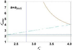
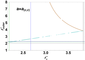
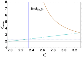
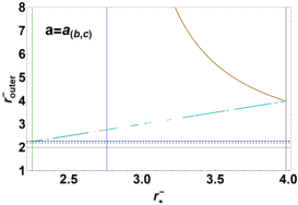
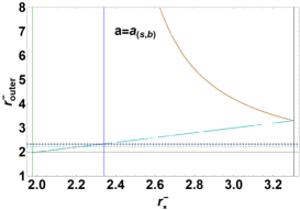
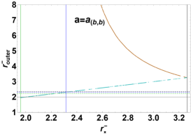
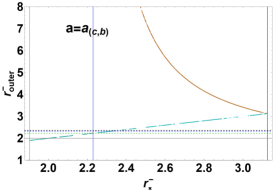
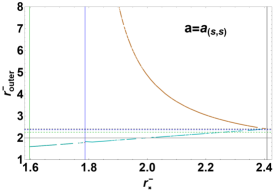
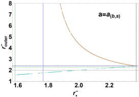
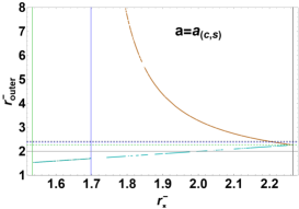
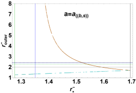
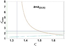
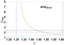
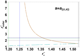
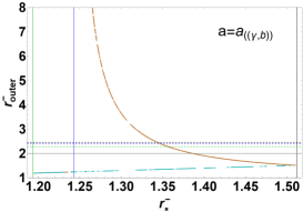
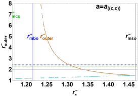
Figure 11: Outer edge $r_{outer}^{-}$ (brown curve) versus cusp $r_{\times}^{-}$ (cyan curve) of the co–rotating cusped disks (and proto-jets) for different spins of Table 2 signed on the panel. Vertical blue (black)(green) line is the marginally bound (stable) (circular) co–rotating orbit $r_{mbo}^{-}$ ($r_{mso}^{-}$) ($r_{mco}^{-}$). All quantities are dimensionless. The outer ergosurface on the equatorial plane is $r=2$ (gray line). Dotted lines are $r_{{\mbox{\scriptsize{{T}}}}}(\ell_{mso}^{+})>r_{{\mbox{\scriptsize{{T}}}}}(\ell_{mbo}^{+})>r_{{\mbox{\scriptsize{{T}}}}}(\ell_{mco}^{+})$, $r_{\mbox{\scriptsize{{T}}}}$ is the inversion radius.

.

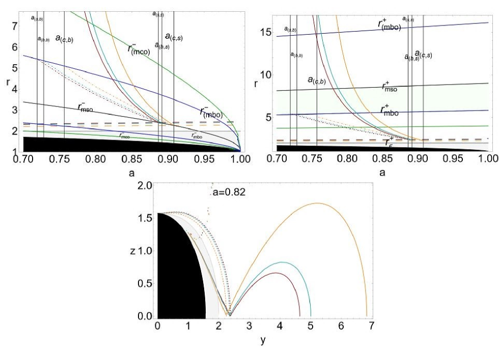
Figure 12: Inversion surfaces crossing the disks cusp. Black region is the central BH, with dimensionless spin $a$. There is $r=\sqrt{y^{2}+z^{2}}$ and $\theta=\arccos({z}/r)$. Gray region is the outer ergoregion (radius $r_{\epsilon}^{+}$ is the outer ergosurface). Dashed lines are the inversion surfaces $r_{\mbox{\scriptsize{{T}}}}$ at fixed counter–rotating angular momentum $\ell^{+}$. Spins signed on the panels (vertical black lines) are defined in Table 2. There is $\mathrm{Q}_{\bullet}$ for any quantity evaluated at $r_{\bullet}$, where $mbo$ (blue curve) is for marginally bound circular orbit, $mco$ (green curve) is for marginally circular orbit, $mso$ (black curve) is for marginally stable circular orbit. In the upper left panel the outer solutions $\ell_{mco}^{-}=\ell^{-}(r)$ (green curve) and $\ell_{mbo}^{-}=\ell^{-}(r)$ (blue curve) are also shown–(see Eqs (14)). $\ell^{-}$ is the co–rotating angular momentum. Red, cyan and orange solid (dotted-dashed) curves are the outer edge (center) correspondent to the solutions of $r_{\times}^{-}=r_{\mbox{\scriptsize{{T}}}}(\ell_{*}^{+})$, where $r_{\times}^{-}$ is here the co–rotating disk or proto-jet cusp and the counter–rotating angular momentum is $\ell_{*}^{+}\in\{\ell_{mco}^{+},\ell_{mbo}^{+},\ell_{mso}^{+}\}$ (orange, cyan and red curves respectively). Upper left panel is a close–up view of the upper right panel. Green region is the location range of the accretion disk cusp. Bottom panel shows the relative tori equi–potential surfaces and the inversion surfaces. All quantities are dimensionless.

.

V.2.2 The co–rotating torus inner edge

We explore the situation where a toroid cusp crosses an inversion surface. In this case the disks are external to the inversion surface as shown in Fig. 12 with the related torus center and outer edge. Constraints, according to the BHs spin, have been also discussed for the BH classes of Table 3. The condition

$$r_{inner}^{-}(\ell^{-},K^{-},a)=r_{\mbox{\scriptsize{{T}}}}(\ell_{\bullet}^{+})$$ (23)

is satisfied for $r_{mbo}^{-}<r_{\mbox{\scriptsize{{T}}}}(\ell_{\bullet}^{+})=r_{\times}^{-}(\ell^{-})<r_{mso}^{-}$, implying $a\in[a_{(\bullet,b)},a_{(\bullet,s)}[$, for the torus cusp, or $r_{mco}^{-}<r_{\mbox{\scriptsize{{T}}}}(\ell_{\bullet}^{+})=r_{J}^{-}(\ell^{-})<r_{mbo}^{-}$, implying $a\in[a_{(\bullet,c)},a_{(\bullet,b)}[$, for the proto-jet cusp, according to the different counter–rotating momenta $\ell_{\bullet}^{+}\in\{\ell_{mco}^{+},\ell_{mbo}^{+},\ell_{mso}^{+}\}$.

However, we should note that for the toroid inner edge it has to be, $r_{inner}^{-}(\ell^{-},K^{-},a)\in[r_{\times}^{-}(\ell^{-}),r_{center}^{-}(\ell^{-})[$ for $\textbf{()}_{1}^{-}$ toroids, $r_{inner}^{-}(\ell^{-},K^{-},a)\in[r_{J}^{-}(\ell^{-}),r_{center}^{-}(\ell^{-})[$ for $\textbf{()}_{2}^{-}$ toroids, and $r_{inner}^{-}(\ell^{-},K^{-},a)<r_{center}^{-}(\ell^{-})$ for $\mathrm{C}_{3}^{-}$ tori. Hence, for a quiescent torus, the inner edge $r_{inner}^{-}(\ell^{-},K^{-},a)$ depends on the torus parameter $K^{-}$, but it is upper bounded by the toroid cusp for $(\textbf{()}_{1}^{-},\textbf{()}_{2}^{-})$ configurations, which is the case considered in this section. However, for the $\mathrm{C}_{3}^{-}$ tori and, more in general, for a quiescent torus, we could consider the upper bound on the inner edge provided by the torus center $r_{center}^{-}$. A torus inner (and outer) edge could possibly be also very close to the torus center up to the limit of a very thin torus, this case will be considered in Sec. (V.2.3).

The disk inner region and the proto-jet range $[r_{J}^{-},r_{center}^{-}]$, decrease with the increasing of the BH spin. See also Fig. 11 and Fig. 13, where Eq. (23) is solved in terms of the co–rotating specific angular momentum $\ell^{-}$, i.e. as solution of the equation $r_{\times}^{-}(\ell^{-})=r_{\mbox{\scriptsize{{T}}}}(\ell_{*}^{+})$, seen as function of the BH dimensionless spin $a$ for different counter–rotating specific angular momentum $\ell_{*}^{+}$ of the inversion surfaces.

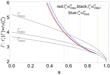
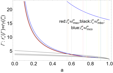
Figure 13: Co–rotating specific angular momentum $\ell^{-}$ solution of the equation $r_{\times}^{-}(\ell^{-})=r_{\mbox{\scriptsize{{T}}}}(\ell_{*}^{+})$, as function of the BH dimensionless spin $a$ for different counter–rotating specific angular momentum $\ell_{*}^{+}$ signed on the panel. There is $\mathrm{Q}_{\bullet}$ for any quantity evaluated at $r_{\bullet}$, where $mbo$ is for marginally bound circular orbit, $mco$ is for marginally circular orbit, $mso$ is for marginally stable circular orbit. $r_{\times}^{-}$ is the cusp of a co–rotating disk or proto-jets. $r_{\mbox{\scriptsize{{T}}}}$ is the inversion radius (where $u^{\phi}$=0). Dotted vertical lines are spins of Table 2. Left panel is a close up vew of the right panel. All quantities are dimensionless.

V.2.3 The co–rotating torus center

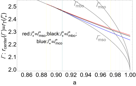
Figure 14: Co–rotating specific angular momentum $\ell^{-}$ solution of the equation $r_{center}^{-}(\ell^{-})=r_{\mbox{\scriptsize{{T}}}}(\ell_{*}^{+})$, as function of the BH dimensionless spin $a$ for different counter–rotating specific angular momentum $\ell_{*}^{+}$ signed on the panel. There is $\mathrm{Q}_{\bullet}$ for any quantity evaluated at $r_{\bullet}$, where $mbo$ is for marginally bound circular orbit, $mco$ is for marginally circular orbit, $mso$ is for marginally stable circular orbit. $r_{center}^{-}$ is the center of a co–rotating disk or proto-jets. $r_{\mbox{\scriptsize{{T}}}}$ is the inversion radius (where $u^{\phi}$=0). (Dotted vertical line are spins of Table 2). All quantities are dimensionless.

.

In Fig. 14 some aspects of the analysis of the co–rotating toroids centers crossing an inversion surface are shown. In general for these systems, the relation

$$r_{center}^{-}(\ell^{-})=r_{\mbox{\scriptsize{{T}}}}(\ell_{\bullet}^{+})$$ (24)

holds. (Note, the toroid center $r_{center}^{-}(\ell^{-})$ depend on the $\ell$ parameter only–see Sec. (III.1).) In Fig. 14 the co–rotating specific angular momentum $\ell^{-}$, solution of Eq. (24), is shown as function of the BH dimensionless spin $a$ for different counter–rotating specific angular momentum $\ell_{\bullet}^{+}$ of the inversion surfaces. Results for $\mathrm{C}_{3}^{-}$ toroids, having momentum in $\mathbf{L_{3}^{-}}$, are also shown. As discussed in Table 3, for the spacetimes classes, co–rotating disks or proto–jets are partially embedded in the inversion surfaces for large BH spin ($a>a_{(b,s)}$) (and can be partially embedded with their centers for $a_{(s,s)}$). For these systems the toroids inner region (including the cusp) is embedded in the inversion surface, while the tori outer region can be external to the inversion surface. However Eq. (24) can also be seen as a limiting case for the configuration where the torus center is internal or external to the inversion surface. As discussed in Sec. (V.2.2) and Sec. (V.2.1), this case will also serve as a constraint for the location of the inner and outer edges of a quiescent torus. A quiescent torus edges depend also on the torus parameter $K^{-}$, and for $K^{-}\geq K_{center}^{-}(\ell^{-})$ the torus can be very small, with the edges close to the disks centers. (This condition can also be verified for cusped tori with momenta $\ell^{-}\geq\ell_{mso}^{-}$.)

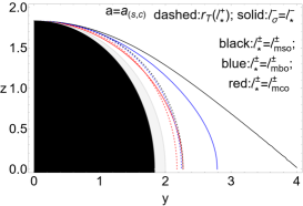
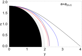
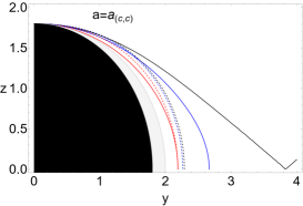
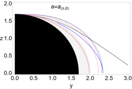
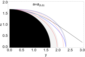
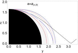
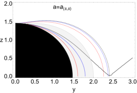
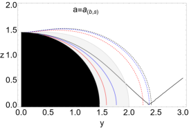
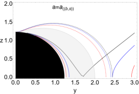
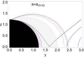
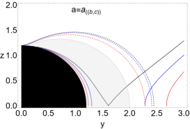
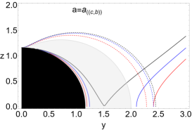
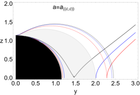
Figure 15: Inversion surfaces crossing the toroids pressure and geometrical extremes. Black region is the central BH, with dimensionless spin $a$. There is where $r=\sqrt{y^{2}+z^{2}}$ and $\theta=\arccos({z}/r)$. Gray region is the outer ergoregion. Dashed curves are the inversion surfaces $r_{\mbox{\scriptsize{{T}}}}$ at fixed counter–rotating angular momentum $\ell^{+}$. Solid curves are the momenta $\ell_{\sigma}^{-}=$constant for co–rotating surfaces defined in Sec. (III.1) connecting the toroids pressure (and density) extremes and geometrical extremes. Spins on the panels are defined in Table 2. There is $\mathrm{Q}_{\bullet}$ for any quantity evaluated at $r_{\bullet}$, where $mbo$ is for marginally bound circular orbit, $mco$ is for marginally circular orbit, $mso$ is for marginally stable circular orbit. All quantities are dimensionless.

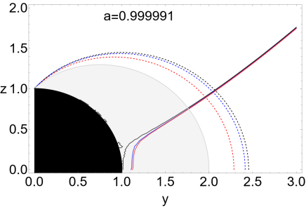
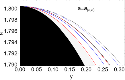
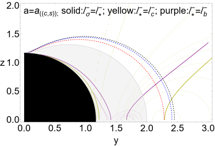
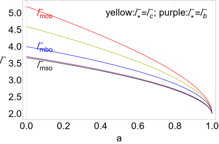
Figure 16: Inversion surfaces crossing the geometrical and density surfaces critical points. Black region is the central BH with dimensionless spin $a$. There is where $r=\sqrt{y^{2}+z^{2}}$ and $\theta=\arccos({z}/r)$. Gray region is the outer ergoregion. Dashed curves are the inversion surfaces, with radius $r_{\mbox{\scriptsize{{T}}}}$, at fixed counter–rotating angular momentum $\ell^{+}$. (For further details see also caption of Fig. 15). Upper line: Analysis of Fig. 15 for spin $a=0.999991$ (left panel), and a close up-view for spin $a=a_{(c,c)}$ (right panel). Below left panel: Analysis of Fig. 15 for spin $a=a_{((c,s))}$ and angular momentum, shown in the right panel as function of $a$, signed on the panel. Dotted lines are the orbiting surfaces. Dashed lines are the inversion surfaces. All quantities are dimensionless.

.

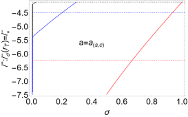
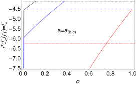
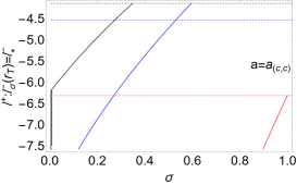
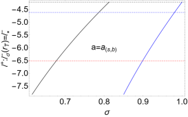
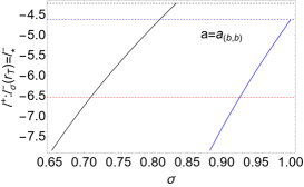
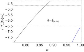
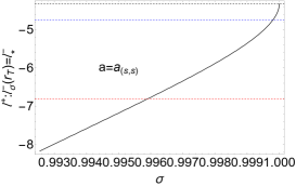
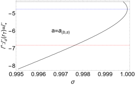
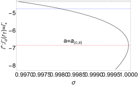
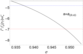
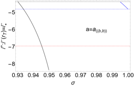
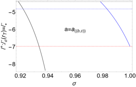
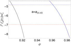
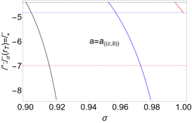
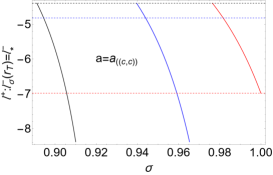
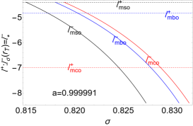
Figure 17: Counter–rotating angular momentum $\ell^{+}$, solution of the equation $\ell_{\sigma}^{-}(r_{\mbox{\scriptsize{{T}}}}(\ell^{+}))=\ell_{\star}^{-}$, versus the angle $\sigma\equiv\sin^{2}\theta\in[0,1]$ for different spins, defined in Table 2, where the co–rotating specific angular momentum $\ell_{\star}^{-}$ is signed on the (bottom) panel. The co–rotating angular momentum $\ell_{\sigma}^{-}$ is defined in Sec. (III.1) . Radius $r_{\mbox{\scriptsize{{T}}}}(\ell^{+})$ is the inversion surface. There is $\mathrm{Q}_{\bullet}$ for any quantity evaluated at $r_{\bullet}$, where $mbo$ is for marginally bound circular orbit, $mco$ is for marginally circular orbit, $mso$ is for marginally stable circular orbit. All quantities are dimensionless. (For further details see also caption of Fig. 15.)

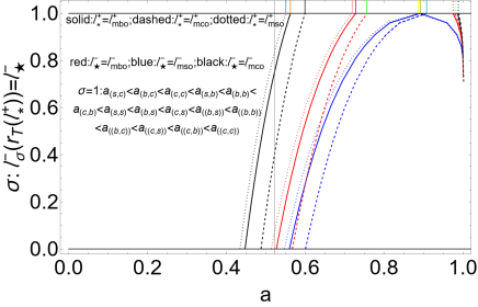
Figure 18: Solution of the equation $\sigma:\ell_{\sigma}^{-}((r_{\mbox{\scriptsize{{T}}}})=\ell_{\star}^{-}$ versus the dimensionless BH spin $a$. There is $\sigma\equiv\sin^{2}\theta\in[0,1]$. The co–rotating angular momentum $\ell_{\sigma}^{-}$ is defined in Sec. (III.1) . $r_{\mbox{\scriptsize{{T}}}}(\ell^{+})$ is the inversion surface radius. Solutions express the angle $\sigma$ for the inversion surface crossing the curves correspondent to the toroids extreme points (centers, cusps and geometrical maxima). The figure shows the solutions for different counter–rotating (co–rotating) angular momentum $\ell_{*}^{+}$ ($\ell_{\star}^{+}$). There is $\mathrm{Q}_{\bullet}$ for any quantity evaluated at $r_{\bullet}$, where $mbo$ is for marginally bound circular orbit, $mco$ is for marginally circular orbit, $mso$ is for marginally stable circular orbit. Solid vertical lines in the region $\sigma>1$ mark the spins defined in Table 2. All quantities are dimensionless.

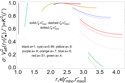
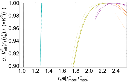
Figure 19: Solution of the equation $\sigma:V_{eff}^{2}((r_{\mbox{\scriptsize{{T}}}},\ell^{-})=K^{2}$ versus the co–rotating disk cusp $r_{\times}$. There is $\sigma\equiv\sin^{2}\theta\in[0,1]$. $V_{eff}$ is the torus effective potential function. There is $K\equiv V_{eff}(r,\ell(r))$. $r_{\mbox{\scriptsize{{T}}}}(\ell^{+})$ is the inversion surface radius. Right panel is a close–up view of the left panel. The figures show the solutions for different counter–rotating angular momentum $\ell_{\star}^{+}$, for different spins signed on the panel. There is $\mathrm{Q}_{\bullet}$ for any quantity evaluated at $r_{\bullet}$, where $mbo$ is for marginally bound circular orbit, $mco$ is for marginally circular orbit, $mso$ is for marginally stable circular orbit. All quantities are dimensionless. Solutions express the crossing of the inversion surface with the co–rotating toroids orbiting the central Kerr BH.

.

It can be $r_{center}^{-}(\mathbf{L_{1}^{-}})<r_{\mbox{\scriptsize{{T}}}}(\mathbf{L_{1}^{+}})$ for $a\in]a_{(s,s)},a_{(b,s)}[$, it can be $r_{center}^{-}(\mathbf{L_{1}^{-}})<r_{\mbox{\scriptsize{{T}}}}(\mathbf{L_{2}^{-}})$ for $a\in]a_{(b,s)},a_{(c,s)}[$, It can be $r_{center}^{-}(\mathbf{L_{1}^{-}})<r_{\mbox{\scriptsize{{T}}}}(\mathbf{L_{3}^{-}})$ for $a\in]a_{(c,s)},a_{((b,s))}[$. Within these conditions it can be also $r_{center}^{-}(\mathbf{L_{2}^{-}})<r_{\mbox{\scriptsize{{T}}}}(\mathbf{L_{1}^{-}})$ for $a\in]a_{((b,s))},a_{((b,b))}[$, while for $a\in]a_{((b,b))},a_{((b,c))}[$ it must be $r_{center}^{-}(\mathbf{L_{1}^{-}})<r_{\mbox{\scriptsize{{T}}}}(\mathbf{L_{1}^{+}})$ other conditions and faster spinning BHs are detailed in Table 3

V.2.4 The critical points of pressure (disks centers and cusps) and the tori geometrical maximum

The toroids critical points of pressure (the extreme points of the effective potential function $V_{eff}$ of Eq. (12)), which are the disks centers and cusps, are located on the equatorial plane, and depend on the parameter $\ell^{-}$ only. The torus geometrical maximum , which is located on plane different from the equatorial, depends on the parameter $\ell^{-}$ only, for the cusped tori $\mathrm{C}_{\times}^{-}$, and on the $(\ell^{-},K^{-})$ parameters for quiescent tori. The critical points of pressure and the geometrical maximum are points of the curve $\ell^{-}_{\sigma}=$constant, where $\ell^{-}_{\sigma}:\partial_{y}V_{eff}^{2}=0$ (for $\{z=r\cos\theta,y=r\sin\theta\sin\phi,x=r\sin\theta\cos\phi\}$), where $\left.\ell_{\sigma}^{-}\right|_{\sigma=1}=\ell^{-}:\left.\partial_{r}V_{eff}\right|_{\sigma=1}=0$, providing, on the equatorial plane, the critical points of pressure–see Fig. 16–bottom left panel.

In this section we constrain the inversion surfaces crossing the tori critical points of pressure and geometrical maximum by considering the solutions of the equation

$$\sigma(a):\ell_{\sigma}^{-}(r_{\mbox{\scriptsize{{T}}}}(\ell^{+}_{\bullet}))=\ell_{\star}^{-}$$ (25)

for different angular momenta $(\ell^{+}_{\bullet},\ell^{-}_{\star})$, versus the dimensionless BH spin $a$. Results are shown in Fig. 18. Solutions provide the angle $\sigma$ where the inversion surface with momentum $\ell^{+}_{\bullet}$ crosses the curves correspondent to extreme points (centers, cusps and geometrical maxima) of the toroids with angular momentum $\ell_{\star}^{-}$.

We also solved Eq. (25), for the counter–rotating angular momentum $\ell^{+}$ of the inversion surfaces, obtaining the solutions

$$\ell^{+}(\sigma):\ell_{\sigma}^{-}(r_{\mbox{\scriptsize{{T}}}}(\ell^{+}_{\bullet}))=\ell_{\star}^{-}$$ (26)

versus the angle $\sigma$ for different spins defined in Table 2, providing the momentum $\ell^{+}_{\bullet}$ of the inversion surface crossing the curves correspondent to extreme points (centers, cusps and geometrical maxima) of the toroids with angular momentum $\ell_{\star}^{-}$. Results are shown in Fig. 17. For a torus with parameter $(\ell^{-},K^{-})$ there is $r^{-}_{inner}(\ell^{-},K^{-})<r_{center}^{-}(\ell^{-})<r_{\max}^{-}(\ell^{-},K^{-})<r_{outer}^{-}(\ell^{-},K^{-})$, where $r_{\max}^{-}(\ell^{-})$ is the projection on the equatorial plane of the torus geometric maximum. In Fig. 15 and Fig. 16 we showed the curves with momenta $\ell_{\sigma}^{-}$ crossing (in the plane $(y,z)$) the inversion surfaces $r_{\mbox{\scriptsize{{T}}}}$ at fixed counter–rotating angular momentum $\ell^{+}$. From Fig. 15 it is clear how the solutions $\ell_{\sigma}^{-}=\ell_{\star}^{-}$ on plane $(y,z)$ are two curves, which are joint on $r=r_{mso}^{-}$ for $\ell_{\star}^{-}=\ell^{-}_{mso}$. The outer curve contains the torus center (on the equatorial plane) and the geometrical maximum (on $\sigma<1$). The inner curve is related to the accretion flows onto BH, and on the equatorial plane it coincides with the toroid cusp (see Fig. 16-bottom right panel). For $\ell_{\star}^{-}=\{\ell^{-}_{mbo},\ell^{-}_{mco}\}$ the outer and inner curves are disjoint. The curves cross the inversion surfaces in the spacetimes with BH spins $a\geq a_{(s,s)}$. From Fig. 15 it is clear that the relevant spins for the inversion surface $r_{\mbox{\scriptsize{{T}}}}(\ell^{+}_{mso})$ are $a_{((\bullet,s))}$ and $a_{(s,s)}$, according to the different co–rotating momenta $\ell_{\bullet}^{-}\in\{\ell_{mco}^{-},\ell_{mbo}^{-}\}$. For the inversion surface $r_{\mbox{\scriptsize{{T}}}}(\ell^{+}_{mbo})$ the discriminant spins are $a_{((\bullet,b))}$ and $a_{(b,s)}$, according to the different co–rotating momenta $\ell_{\bullet}^{-}\in\{\ell_{mco}^{-},\ell_{mbo}^{-}\}$, indicating the spacetimes characterized by the crossing of the inversion surfaces with the curves of tori pressure and geometrical extremes for fixed momenta $\ell^{\pm}$, and for the inversion surface $r_{\mbox{\scriptsize{{T}}}}(\ell^{+}_{mco})$ we note the role of the BH spins $a_{((\bullet,c))}$ and $a_{(c,s)}$. On the other hand, focusing on the co–rotating toroids curves $\ell_{\sigma}^{-}=\ell_{\star}^{-}=\ell^{-}_{mso}$, spins $a_{(\bullet,s)}$ (for the different counter–rotating momenta $\ell_{\bullet}^{+}\in\{\ell_{mco}^{+},\ell_{mbo}^{+},\ell_{mso}^{+}\}$) are relevant for the crossings with the inversion surfaces, while the spin for the curves for $\ell_{\star}^{-}=\ell^{-}_{mbo}$ there are the limiting spins $a_{((b,\bullet))}$. For $\ell_{\star}^{-}=\ell^{-}_{mco}$, there are the spins $a_{((c,\bullet))}$, limiting for the crossings with the co–rotating surfaces with $\ell^{-}=\ell^{-}_{mco}$. The surfaces $\ell_{\sigma}^{-}=\ell_{\star}^{-}$ are very close for faster spinning BHs (Fig. 16–upper left panel). The inner curves regulate therefore also the accretion flows with respect to the inversion surfaces close to the BH poles (see Fig. 16–upper right panel). For materials accreting into the central Kerr BH the toroidal velocity of the $u$counter–rotating accretion flows changes sign on the inversion surfaces. It is evident from Fig. 17 the discriminant rule of the spins $a_{(\bullet,s)}$, relating $\ell^{\pm}$ of the inversion surfaces and the co–rotating toroids respectively.

V.2.5 The off–equatorial crossing of the co–rotating toroids with an inversion surface

In this section we investigate the co–rotating cusped toroids (proto-jets and tori) partially contained in an inversion surface, considering the toroids crossing the inversion surfaces on planes different from the equatorial. Part of this problem has been faced in Sec. (V.2.5), where we concentrated on the torus geometrical maximum. In here, we narrow the analysis to cusped co–rotating toroids. Results of this analysis are in Figs 18,19 and Figs 15,16,17.

In Fig. 19 we show the angles $\sigma$, solutions of the equation:

$$\sigma:V_{eff}^{2}((r_{\mbox{\scriptsize{{T}}}}(\ell_{\star}^{+}),\ell^{-}(r_{\times}^{-}))=K^{2}_{\times}$$ (27)

versus the disk cusp $r_{\times}^{-}\in[r_{mbo}^{-},r_{mso}^{-}]$, for different counter–rotating angular momentum $\ell_{\star}^{+}$ defining the inversion surfaces, for different spins signed on the panels. Solutions are the angles $\sigma$ at the crossing of the inversion surface with the co–rotating cusped tori $\mathrm{C}_{\times}^{-}$ orbiting the central BH. We note that different situations emerge for the faster and slower attractors.

Radii $\{r_{center}^{-},r_{\times}^{-},r_{J}^{-},r^{-}_{\max}\}$, where $r^{-}_{\max}$ is the geometrical maximum projection on the equatorial plane, are related by the curves $\ell_{\sigma}^{-}=$constant, where, on the equatorial plane, there is $\left.\ell_{\sigma}^{-}\right|_{\sigma=1}=\ell^{-}$. Fig. 18 shows the angles $\sigma(a)$, solutions of the equation $\ell_{\sigma}^{-}(r_{\mbox{\scriptsize{{T}}}}(\ell^{+}_{\bullet}))=\ell_{\star}^{-}$ as function of the dimensionless BH spin $a$, where the inversion surfaces with momentum $\ell^{+}_{\bullet}$ cross the curves correspondent to the geometrical maxima and the pressure critical points of the toroids with angular momentum $\ell_{\star}^{-}$. Solutions for the counter–rotating angular momentum $\ell^{+}(\sigma)$ of the inversion surfaces, versus the angle $\sigma$ are shown for different spins in Fig. 17. The geometrical maximum represents a limiting value of the toroidal surface crossing the inversion surface in the inner or outer region.

VI Conclusion

Co–rotating toroids and proto-jets, orbiting a Kerr BH, can be embedded, external or partially contained in the spacetimes inversion surfaces, according to the BHs spins and the counter–rotating flows specific angular momentum. The inversion surfaces are located out of the outer ergoregion of the Kerr BH spacetime, and they are defined for counter–rotating flows only, having specific angular momentum $\ell<0$. We showed that a counter–rotating toroid is always external to the inversion surfaces for counter–rotating flows and inversion surfaces specific angular momentum sufficiently large in magnitude, i.e. $\ell^{+}<\ell_{mso}^{+}$. The constraints on the inversion surfaces with lower specific angular momentum in magnitude, crossing an outer counter–rotating toroid are provided in Sec. (V.1). The constraints define the limiting angular momentum $\ell_{G}^{+}$ of Eq. (19) for the counter–rotating flows (see Fig. 9). Therefore in this analysis we concentrated on the counter–rotating (and $u$counter–rotating) flows inversion surfaces of the Kerr spacetimes in relation to the (inner) co–rotating toroids.

Toroids are found as equi–potential surfaces from the scalar function $V_{eff}$ of Eq. (12) with constant specific angular momentum.

In this analysis we have heavily relied on the fact that the inversion surface (defined as the loci of the vanishing toroidal flow velocity) and the surface separating the co-rotating and counter-rotating toroids, do not coincide. This is in fact an essential aspect constituting the premise of this analysis, leading to the possibility that the fluid coming from an external counter-rotating disk can impact on a inner co-rotating disk with different conditions on the fluids toroidal velocity components. If the disks orbit very far from the attractor, for example having specific angular momentum parameter $\ell^{\pm}\in\mathbf{L}_{3}^{\pm}$, there can be no separation regions: the outer torus of the pair could be for example a quiescent co–rotating torus. On the other hand, focusing on the pair composed by an external counter-rotating cusped disk and an internal co-rotating disk, the tori separation region is bounded above by $r_{mbo}^{+}$. (In the case of quiescent tori or proto-jets the situation is different.) Therefore, this limit is fixed exclusively by the spin of the attractor. Then, the maximum radius of extension of the co-rotating disk, is bounded by the maximum extension of the disk outer edge, which is evaluated in this analysis accurately in Sec. (V.2.1) and illustrated, for example, in Figs (10). It general it has to be $r_{outer}^{-}>r_{mso}^{-}$. The case of inter–disks inversion sphere evidently occurs when $r_{\mbox{\scriptsize{{T}}}}\in]r_{outer}^{-},r_{inner}^{+}[$, which is well clarified from Figs (7). These considerations are reported for the equatorial plane, since the toroids are both orbiting on the equatorial plane of the central attractor. However, the inter–disks inversion sphere has a role also in the off–equatorial dynamics between the two toroids. This aspect is relevant, since the tori considered in this analysis are geometrically thick. This situation is treated in Sec. (V.2.5). This difference between the inversion surface and the tori separation regions leads to three different scenarios for tori embedded in an inversion surface, toroids located out of the inversion surface or crossing the inversion surfaces in particular points being partially contained in the inversion surface.

All the co–rotating toroids orbiting in the BH outer ergoregion are embedded in all the inversion surfaces and will be “shielded” from contact with the $u$counter–rotating flows. In general, however, the inversion surfaces are defined by a general, necessary but not sufficient, condition on (the photons and) matter which can be ingoing into the BH, or outgoing or also moving along the BH spinning axis. On the other hand, the $u$counter–rotating flows accreting into the central BH, have inversion points, crossing the inversion surfaces defined by the flow (conserved) specific angular momentum $\ell<0$. Thus, a co–rotating toroid, entirely contained in this inversion surface, is “shielded” from impact with the $u$counter–rotating materials with constant specific angular momentum $\ell<0$, accreting into the central BH (the flow being $u$co–rotating after crossing the flow inversion surfaces). Although the inversion surfaces have a more general significance, in this case the effects of the flow inversion surfaces emerge as a consequence of the spacetime frame–dragging. This is the case considered here for the inter–disks inversion surfaces, when the $u$counter–rotating flows coming from the outer accreting counter–rotating disk into the central BH, impact on an inner co–rotating toroid. We also studied the case where one or two orbiting structures are proto–jets (inter proto-jets inversions surfaces), providing the conditions when a co–rotating disk or co–rotating proto–jet can be replenished with $u$counter–rotating matter and photons which is accreting into the central BH or, viceversa, when the counter–rotating matter and photons impacting on the surface will be $u$co–rotating, constrained according to the flow parameters $\ell^{\pm}$ and the BH spin dimensionless $a$.

In Table 1 the constraints on the flows and orbiting toroids, discussed in Sec. (III), are summarized. We based part of our analysis on the assumption that an equatorial accretion disk inner edge is located in the range $[r_{mbo}^{\pm},r_{mso}^{\pm}]$ (for counter–rotating and co–rotating disks respectively). The analysis of the co–rotating toroids in relation to the spacetime inversion surfaces, developed in Sec. (V.1), lead to distinguish sixteen classes of BH spacetimes according to the BH spins defined in Table 2 and shown in Figs 6,7,8. (Boundary spins in Table 2 result from the intersection between the inversion surfaces radii $r_{\mbox{\scriptsize{{T}}}}(\ell^{+}_{\bullet})$ with the co–rotating extended geodesic structure –see Figs 7,8.) The inversion surfaces properties in each spacetime class are summarized in Table 3, where each class is characterized by the occurrence of a given inter–disks inversion surfaces, or constrained, in terms of the parameters $(\ell^{\pm},K^{-},a)$, by the possibility of a given configuration. We found that, in the spacetimes with spin $a\in]0,a_{(s,c)}]$ the inversion surfaces are always internal to the outer co–rotating toroids. The centers $r_{center}^{-}$ are external to the inversion surfaces, in the spacetimes with spins $a\leq a_{(s,s)}$. For $a\in]a_{(s,c)},a_{(c,s)}[$, tori can be only partially included in an inversion surface. Therefore, for $a<a_{(s,s)}$ co–rotating toroids could be only partially included (with the inner region) in an inversion surface. In this range a disk or proto-jet cusp could be internal or external to an inversion surface. For $a\geq a_{(s,s)}$ the toroid center can be contained in an inversion surface, and therefore in these spacetimes a torus can be entirely embedded in the inversion surface, for small co–rotating specific angular momentum $\ell^{-}$. For $a>a_{(s,s)}$ quiescent tori or, for the faster spinning attractors, cusped tori, can be or are internal to the inversion surfaces , according to the conditions in Table 3–some of these tori are in the ergoregion. When $a\geq a_{((\bullet,\star))}$ (and from $a\geq a_{(s,s)}$ with more constraints), according to the specific angular momenta $\ell_{\bullet}^{+}\in\{\ell_{mco}^{+},\ell_{mbo}^{+},\ell_{mso}^{+}\}$, a co–rotating torus could be entirely embedded in an inversion surface.

Hence, in Sec. (V.2) we investigated the inversion surfaces crossing the co–rotating toroids by examining specifically in Sec. (V.2.1) the crossing with the toroids outer edges. Results are illustrated in Fig. 10 and Fig. 11. In this case, the toroids with the outer edge crossing an inversion surface are entirely embedded in the inversion surfaces and therefore can be totally shielded from impact from $u$counter–rotating flows accreting into the BH with the constant specific angular momentum. The crossing can occur for large BH spin and small momenta in magnitude of the inversion surface. Tori with $\ell\in\mathbf{L_{1}^{-}}$ satisfy this condition in the spacetimes with spins $a>a_{(\bullet,s)}$ (for $a_{(\bullet,s)}=\{a_{(s,s)},a_{(b,s)},a_{(c,s)}\}$ according to the different angular momentum).

For co–rotating toroids with specific angular momenta $\ell^{-}\in\mathbf{L_{2}^{-}}$ we restricted the spacetimes to the spins $a>a_{((b,\bullet))}$–for $a_{((b,\bullet))}=\{a_{((b,s))},a_{((b,b))},a_{((b,c))}\}$ (see Fig. 10–upper left panel). For the quiescent tori with $\ell^{-}\in\mathbf{L_{3}^{-}}$, these cases occur for $a>a_{((c,\bullet))}$ for $a_{((c,\bullet))}=\{a_{((c,s))},a_{((c,b))},a_{((c,c))}\}$.

Flows inversion surfaces crossing the toroids cusp, as shown in Fig. 12, has been discussed in Sec. (V.2.2). In this case the toroids are external to the flow inversion surfaces at fixed specific angular momentum. Results are illustrated in Fig 12 and constrained in Table 3. We proved that, in general this condition can occur for (cusped) co–rotating tori orbiting BHs with spin in the range $a\in[a_{(\bullet,b)},a_{(\bullet,s)}[$ (for the torus cusp) and, for the co–rotating proto-jet cusps in the spacetimes with spin in the range $a\in[a_{(\bullet,c)},a_{(\bullet,b)}[$ (according to the counter–rotating specific angular momenta $\ell_{\bullet}^{+}\in\{\ell_{mco}^{+},\ell_{mbo}^{+},\ell_{mso}^{+}\}$).

When the flows inversion surfaces cross the toroids centers, the toroids are partially contained in the inversion surfaces. This case has been discussed in Sec. (V.2.3) and illustrated in Fig. 14. We proved that it can be $r_{center}^{-}(\mathbf{L_{1}^{-}})<r_{\mbox{\scriptsize{{T}}}}(\mathbf{L_{1}^{+}})$ in the spacetimes with spin $a\in]a_{(s,s)},a_{(b,s)}[$ (detailed constraints, for each spacetimes class, are summarized in Table 3). Disks and proto–jets can be partially embedded in the inversion surfaces for large BH spin ($a>a_{(s,s)}$) and for the faster spinning BHs (as $a<a_{((c,c))}$), the toroids centers will be contained in the inversion surfaces.

More in general we analyzed the inversion surfaces crossing the toroids critical points of pressure and geometrical maxima as points of the curves $\ell^{-}_{\sigma}=$constant. This analysis is discussed in Sec. (V.2.4). Results are illustrated in Fig. 15 and Fig. 16.

Then, the angles $\sigma$, where the inversion surfaces, with fixed specific angular momentum $\ell^{+}$, cross the curves of the toroids extreme points are in Fig. 18, while the inversion surfaces momentum $\ell^{+}$ is shown in in Fig. 17. We proved that the crossing with the inversion surface $r_{\mbox{\scriptsize{{T}}}}(\ell^{+}_{mso})$ occurs in the spacetimes with spins $a_{((\bullet,s))}$ and $a_{(s,s)}$ (according to the different co–rotating momenta $\ell_{\bullet}^{-}\in\{\ell_{mco}^{-},\ell_{mbo}^{-}\}$). For the inversion surface $r_{\mbox{\scriptsize{{T}}}}(\ell^{+}_{mbo})$, a crossing occurs in the spacetimes with spin $a_{((\bullet,b))}$ and $a_{(b,s)}$. For the inversion surface $r_{\mbox{\scriptsize{{T}}}}(\ell^{+}_{mco})$ there are the spins $a_{((\bullet,c))}$ and $a_{(c,s)}$. Spins $a_{(\bullet,s)}$ (for different counter–rotating momenta $\ell_{\bullet}^{+}\in\{\ell_{mco}^{+},\ell_{mbo}^{+},\ell_{mso}^{+}\}$) constrain the spacetimes characterized by the curves $\ell_{\sigma}^{-}=\ell_{\star}^{-}=\ell^{-}_{mso}$ crossings the inversion surfaces. Whereas, for the crossings with the extreme points curves $\ell_{\star}^{-}=\ell^{-}_{mbo}$, there are the limiting spins $a_{((b,\bullet))}$, and for $\ell_{\star}^{-}=\ell^{-}_{mco}$, there are spins $a_{((c,\bullet))}$. (All boundary spins distinguished in this analysis are defined in Table 2.)

On the other hand, the off–equatorial crossing is often the case for the partially contained toroids. The off–equatorial properties are determined by the characteristics of the specific accretion disk model and regulated by the inversion surfaces characteristics, which are fixed exclusively by the background geometry. The inversion surfaces crossing the toroids on planes different from the equatorial have been considered in Sec. (V.2.5) and the results of this analysis were illustrated Figs 18,19 and Figs 15,16,17, summarizing the main aspects of the crossings at different parameters values: we showed the angles $\sigma$ where the inversion surface crosses the co–rotating cusped tori $\mathrm{C}_{\times}^{-}$ in Fig. 19; the angles $\sigma(a)$, where the inversion surfaces with momentum $\ell^{+}_{\bullet}$ cross the curves correspondent to the geometrical maxima and the pressure critical points of the toroids with angular momentum $\ell_{\star}^{-}$ were showed in Fig. 18. Solutions for the counter–rotating angular momentum $\ell^{+}(\sigma)$ of the inversion surfaces, versus the angle $\sigma$ were illustrated, for different spins, in Fig. 17.

Finally we expect that the observational properties on the inversion surfaces could depend strongly on the processes time–scales as related to the time flow reaches the inversion points. However, the inversion surfaces could be a remarkably active part of the accreting flux, particularly in the region of the BH poles (where the inversion surfaces are very close) and the equatorial plane (when the accretion flows mostly leaves the equatorial accretion disks inner edges) and, eventually characterized by an increase of the flow luminosity and temperature.

Data availability

There are no new data associated with this article. No new data were generated or analysed in support of this research.

References

- Pugliese&Stuchlík [2022] Pugliese D.&Stuchlík Z., 2022, MNRAS, 512, 4, 5895–5926
- Pugliese & Stuchlík [2023a] Pugliese D., Stuchlík Z., 2023a, EPJC, 83, 242.
- Pugliese & Stuchlík [2023b] Pugliese D., Stuchlík Z., 2023b, NuPhB, 992, 116229.
- Pugliese & Stuchlík [2024] Pugliese, D., Stuchlík, Z. Eur. Phys. J. C 84, 158 (2024).
- Murray et al. [1999] Murray J. R., de Kool M., Li J., 1999, ApJ, 515, 738
- Kuznetsov et al. [1999] Kuznetsov O. A., et al., 1999, ApJ, 514, 691
- Impellizzeri et al. [2019] Impellizzeri C. M. V., et al., 2019, ApJL, 884, L28
- Ensslin [2003] Ensslin T. A., 2003, Astron. Astrophys. 401, 499-504
- Beckert&Falcke [2002] Beckert T.&Falcke H., 2002, Astron. Astrophys. 388, 1106
- Kim et al. [2016] Kim M. I., Christian D. J., Garofalo D.& D’Avanzo J., 2016, MNRAS 460, 3, 3221–3231
- Barrabes et al. [1995] Barrabes C., Boisseau B. and Israel W. 1995, MNRAS, 276, 432
- Evans et al. [2010] Evans, D. A., Reeves, J. N., Hardcastle, M. J., et al. 2010, Astrophys. J. , 710, 859.
- Christodoulou et al. [2017] Christodoulou D. M., Laycock S. G. T., Kazanas D., 2017, MNRAS: Letters, 470, 1, L21–L24
- Nixon et al. [2011] Nixon C. J., Cossins P. J. , King A. R., Pringle J. E. 2011, MNRAS, 412, 3, 1591–1598
- Garofalo [2013] Garofalo D. 2013.,Advances in Astronomy, 2013, 213105
- Volonteri [2010] Volonteri, M. 2010, Accretion and Ejection in AGN: a Global View, 427, 3
- Volonteri et al. [2003] Volonteri M., Haardt F.,& Madau P., 2003 Astrophys. J. , 582 559
- Nixon et al. [2012a] Nixon, C. J., King, A. R.,&Price, D. J. 2012a, MNRAS, 422, 2547.
- Amaro-Seoane et al. [2016] Amaro-Seoane, P., Maureira-Fredes, C., Dotti, M., et al. 2016, A&A, 591, A114
- Zhang et al. [1997] Zhang S. N., Cui W., Chen W., 1997, ApJ, 482, L155
- Rao&Vadawale [2012] Rao A.&Vadawale S.V., 2012, ApJL, 757, L12
- Reis et al. [2013] Reis R. C. et al., 2013, ApJ, 778, 155
- Middleton et al. [2014] Middleton M. J.,Miller-Jones J. C. A., Fender R. P. 2014, MNRAS, 439, 2, 1740–1748
- Morningstar et al. [2014] Morningstar W. R., Miller J. M., Reis R. C. et al. 2014,Astrophys. J. , 784, L18
- Cowperthwaite&Reynolds. [2012] Cowperthwaite P. S.&Christopher S. R., 2012, ApJL, 752, L21
- Dyda et al. [2015] Dyda S., Lovelace R. V. E, et al., 2015,
- Garofalo et al. [2010] Garofalo D., Evans D.A., Sambruna R. M. 2010, MNRAS, 406, 975-986
- Event Horizon Telescope Collaboration et al. [2019] Event Horizon Telescope Collaboration, Akiyama K., Alberdi A., Alef W., Asada K., Azulay R., Baczko A.-K., et al., 2019, ApJL, 875
- Alig et al. [2013] Alig C., Schartmann M., Burkert A. , Dolag K. 2013, Astrophys. J. , 771, 2, 119
- Carmona-Loaiza et al. [2015] Carmona-Loaiza J.M., Colpi M., Dotti M. et al., 2015,MNRAS,453,1608
- Pugliese&Stuchlík [2015] Pugliese D.&Stuchlík Z., 2015, Astrophys. J.s, 221, 2, 25
- Pugliese&Stuchlik [2018b] Pugliese D.&Stuchlík Z. 2018b,Class. Quant. Grav. 35, 18, 185008
- Pugliese&Stuchlik [2018a] Pugliese D.&Stuchlik Z., 2018a, JHEAp, 17 1
- Kataoka et al. [2007] Kataoka J. et al., 2007, PASJ, 59, 279
- Nixon et al. [2013] Nixon, C., King, A. & Price, D.. 2013, MNRAS, 434, 1946
- Doğan et al. [2015] Doğan, S., Nixon, C., King, A.et al. 2015, MNRAS, 449, 1251
- Bonnerot et al. [2016] Bonnerot C., Rossi E.M., Lodato G. et al. 2016, MNRAS, 455, 2, 2253
- Aly et al. [2015] Aly, H., Dehnen, W., Nixon, C.& King, A., 2015, MNRAS, 449, 1, 65
- Narayan et al. [2022] Narayan R., Chael A., Chatterjee K., Ricarte A., Curd B., 2022, MNRAS, 511
- Tejeda et al. [2017] Tejeda E., Gafton E., Rosswog S., Miller J. C., 2017, MNRAS, 469, 4483
- Wong et al. [2021] Wong G. N. et al., 2021, The Astrophysical Journal, 914:55
- Porth et al. [2021] Porth O., Mizuno Y., Younsi Z., Fromm C. M., 2021, MNRAS, 502, 2023
- Zhang et al. [2015] Zhang W. et al., 2015,The Astrophysical Journal, 807:89
- Bardeen & Petterson [1975] Bardeen, J.M., Petterson, J.A., 1975, Astrophys. J. , 195, L65
- King et al. [2005] King A. R., Lubow S. H., Ogilvie G. I.,& Pringle J. E. 2005 MNRAS, 363, 49
- King&Nixon [2018] King A. and Nixon C., 2018, Astrophys. J. 857, 1, L7.
- King et al. [2008] King A. R., Pringle J. E. & Hofmann J. A.. 2008, MNRAS, 385, 1621
- Lodato & Pringle [2006] Lodato G. & Pringle J. E. 2006, MNRAS, 368, 1196
- Martin et al. [2014] Martin R. G., Nixon C., Lubow S. H., et al. 2014, Astrophys. J. 792, L33
- Nealon et al. [2015] Nealon R., Price D. and Nixon C.,2015, Mon. Not. Roy. Astron. Soc. 448, 2, 1526
- Nixon et al. [2012b] Nixon C. J., King A. R.,& Price D. J., et al.2012b, Astrophys. J., 757, L24
- Scheuerl&Feiler [1996] Scheuerl P. A. O.& Feiler R. 1996, MNRAS, 282, 291-294
- Pugliese&Montani [2015] Pugliese D.& Montani G. 2015, Phys. Rev. D, 91, 8, 083011
- Pugliese&Stuchlík [2016] Pugliese D.&Stuchlík Z., 2016, Astrophys. J.s, 223, 2, 27
- Pugliese&Stuchlík [2017a] Pugliese D.&Stuchlík Z., 2017a, Astrophys. J.s, 229, 2, 40
- Pugliese&Stuchlik [2017b] Pugliese D.&Stuchlík Z., 2017b, Eur. Phys. J. C, 79, 4, 288
- Pugliese&Stuchlik [2018c] Pugliese D.&Stuchlík Z. 2018c Class. Quant. Grav., 35, 10, 105005
- Pugliese&Stuchlik [2021c] Pugliese D.&Stuchlík Z., 2021c, PASJ, 73, 5, 1333-1366
- Pugliese&Montani [2018] Pugliese D.& Montani G. 2018, MNRAS, 476, 4, 4346-4361
- Pugliese&Stuchlik [2021a] Pugliese D.&Stuchlík Z. 2021a, Class. Quant. Grav., 38, 14, 145014
- Pugliese&Stuchlik [2020a] Pugliese D.& Stuchlik Z. 2020a, MNRAS., 493, 3, 4229–4255
- Abramowicz&Fragile [2013] Abramowicz, M. A.& Fragile P. C., 2013, Living Rev. Relativity, 16, 1
- Pugliese&Stuchlik [2020b] Pugliese D.& Stuchlik Z., 2020b, Class.Quant.Grav., 37, 19, 195025
- Carter [1968] Carter B., 1968, Phys. Rev., 174, 1559
- Bardeen, Press, & Teukolsky [1972] Bardeen J. M., Press W. H., Teukolsky S. A., 1972, ApJ, 178, 347.
- Paczyński [1980] Paczyński, B. 1980, Acta Astron., 30, 4
- Igumenshchev [2000] Igumenshchev, I. V. & Abramowicz, M. A., 2000, APJS, 130, 463
- Shafee et al. [2008] Shafee, R., McKinney, J. C, Narayan, R. et al.2008, Astrophys. J. , 687, L25
- Fragile et al. [2007] Fragile, P. C., Blaes, et al., 2007, Astrophys. J., 668, 417-429
- De Villiers&Hawley [2002] De Villiers J-P.& Hawley J. F., 2002. Astrophys. J. , 577, 866