Communication Constellation Design of Minimum Number of Satellites with Continuous Coverage and Inter-Satellite Link

Abstract

Recently, the advancement of research on distributed space systems that operate a large number of satellites as a single system urges the need for the investigation of satellite constellations. The communication constellation can be used to construct global or regional communication networks using inter-satellite and ground-to-satellite links. This paper studies the two challenges of the communication constellation, continuous coverage and inter-satellite link connectivity. The bounded Voronoi diagram and APC decomposition are presented as continuous coverage analysis methods. For the continuity analysis of the inter-satellite link, the relative motion between the adjacent orbital planes derives the analytic solutions. The Walker-Delta constellation and common ground-track constellation design methods are introduced as examples to verify the analysis methods. The common ground-track constellation is classified into a quasi-symmetric and optimal constellation. The optimal common ground-track constellation is optimized by the BILP algorithm. As a result, the simulation results compare the performance of the communication constellations according to various design methods.

1 Introduction

In recent years, the feasibility of low Earth orbit communication satellites has attracted attention due to the trend of small satellites. The examples include Space-X’s Starlink, Eutelsat’s OneWeb, and Amazon’s Kuiper project[1]. Their orbits are designed to provide communication links across the whole Earth. A satellite constellation operates several satellites with distinct orbits as a single system. Compared to conventional geostationary satellites, low Earth orbit satellites have a smaller coverage size and shorter orbital periods, which results in degraded spatial and temporal coverage performance. Therefore, the low Earth orbit constellations operate several satellites to overcome this limitation while minimizing the number of satellites. If the coverage is continuous for the area of interest, the communication constellation can continuously provide communication links. In addition, when the inter-satellite links are connected, the link is not disconnected even by the orbital motion of the satellite and the Earth’s rotation effect. In this paper, the low Earth orbit communication constellation design problem is interpreted as the problem of achieving continuous coverage and inter-satellite links.

The sections are presented in order of constellation design methods, coverage analysis methods, relative motion in adjacent orbital planes, simulation results, and conclusion. The constellation design methods describe the basis of Walker and common ground-track constellations. The Walker constellation first introduces the concept of seed satellite and design parameters and defines the orbital elements. The pattern repetition period and duplicate allocation of orbital elements are explained as two important characteristics of the Walker-Delta constellation and expressed by the design parameters. The repeat ground-track orbit is the seed satellite’s orbit for the common ground-track constellation. The quasi-symmetric method configures the satellites so that the spacings between the adjacent satellites are almost equal. The BILP method optimizes the satellite’s configuration to satisfy the coverage requirement while minimizing the total number of satellites. The coverage analysis methods section first explains a useful concept, the geometry of Earth coverage. Then, Voronoi tessellation and APC decomposition are described with the references. The relative motion in adjacent orbital planes derives key formulae to analyze the bounds of the relative distance. The simulation results present the continuous coverage analysis for Walker-Delta, quasi-symmetric, and BILP constellations and inter-satellite link continuity analysis for three constellations. The last section summarizes and concludes the contents of this paper.

2 Constellation Design Methods

2.1 Walker Constellation

The Walker constellation is the geometric design method that configures the orbits symmetrically[2, 3]. The seed satellite is the one that determines the common orbital elements of the constellation. For the Walker constellation, the satellites are configured in circular orbits with the equal semi-major axis ($a$), inclination ($i$), and argument of perigee ($\omega$) of the seed satellites. The two types of Walker constellations are classified depending on the inclination. The Walker-Star constellation is designed based on the polar orbit and achieves global coverage. The Walker-Delta constellation, on the other hand, has an inclination under 90 degrees and covers the mid-latitude and equator region. Therefore, this classification is only relevant to the latitude of the area of interest (AoI).

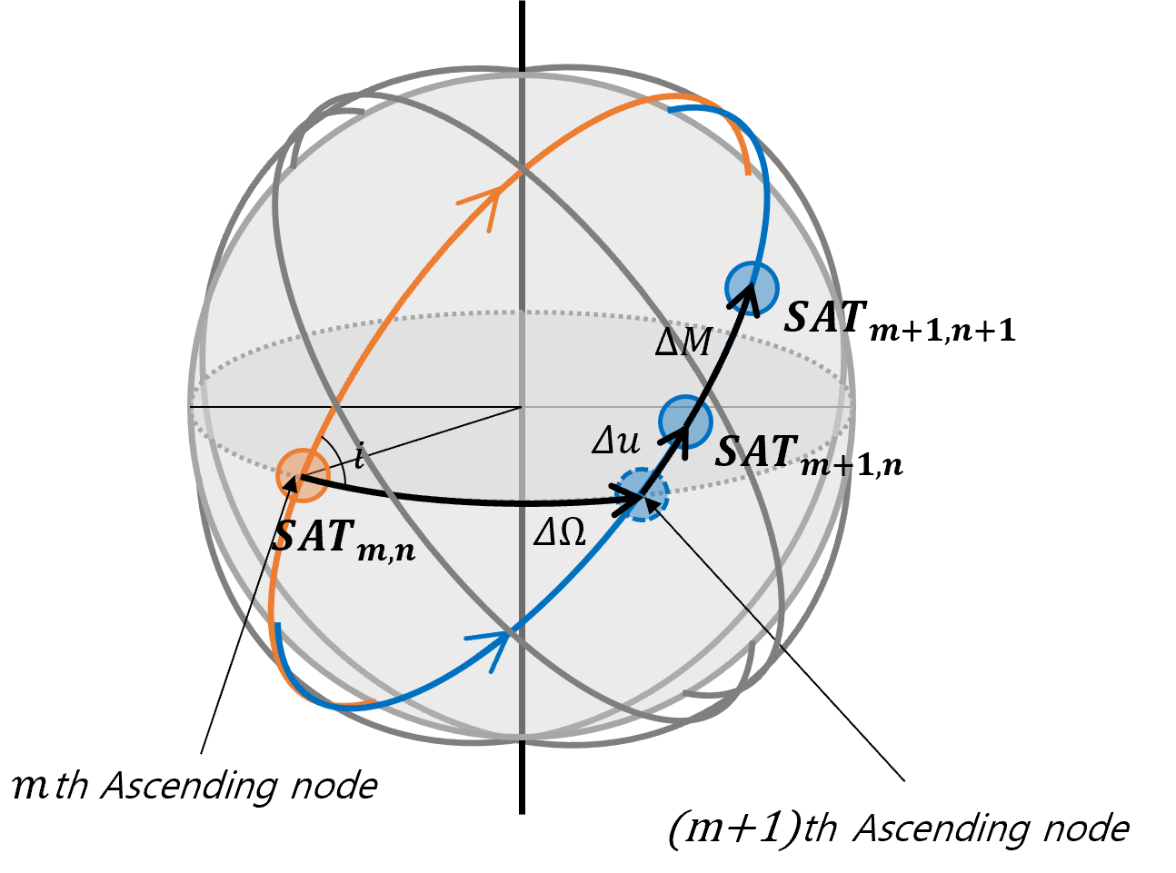
Figure 1: Geometric description of Walker-Delta constellation orbital elements

The three design parameters are the total number of satellites ($T$), the number of orbital planes ($P$), and the phasing parameter ($F\in\{0,1,...,P-1\}$). The number of satellites per orbital plane ($S=T/P$) is an auxiliary parameter to prevent confusion. The right ascension of ascending node (RAAN, $\Omega_{m}$) and the mean anomaly ($M_{m,n}$) of the $n$th satellite in the $m$th orbital plane ($SAT_{m,n}$) are defined as Eqs. (1) and (2) and depicted in Figure 1.

$$\Omega_{m}=\frac{360}{P}\cdot\left(m-1\right)\deg$$ (1)

$$M_{m,n}=\frac{360}{T}\cdot F\cdot\left(m-1\right)+\frac{360}{S}\cdot\left(n-1\right)\deg$$ (2)

where $m=1,2,...,P$ and $n=1,2,...,S$.

From the equation (1), the RAAN is equally spaced by $\Delta\Omega=360/P\deg$ in the range of $\Omega_{m}\in\left[0,360\right]\deg$. The intraplane spacing $\Delta M=360/S\deg$ generates the symmetric location in the orbital plane in the range of $M\in\left[0,360\right]\deg$ and is equivalent to the relative angular distance between the satellites in the orbital plane. The relative argument of latitude ($\Delta u$) in the adjacent orbital planes is derived as $\Delta u=360/T\cdot F\deg$ from Eq. (2).

2.1.1 Pattern Repetition Period

The Walker-Delta pattern has the geometric characteristics that the intra- and inter-plane angular spacings are uniform. This geometric symmetricity determines the pattern repetition period. The investigation of the patterns in the geographical coordinate system enhances understanding of the pattern repetition period. The reference [4] derived the formulae of pattern repetition period. The pattern unit (PU) more briefly describes the orbital elements of Walker-Delta constellation. The definition of the pattern unit is as below[2, 3]:

$$1\text{PU}=\frac{360}{T}\deg$$ (3)

The RAAN and mean anomaly in Eqs. (1) and (2) are reorganized in pattern unit as

$$\Omega_{m}=S\cdot\left(m-1\right)\text{PU}$$ (4)

$$M_{m,n}=F\cdot\left(m-1\right)+P\cdot\left(n-1\right)\text{PU}$$ (5)

The time interval that the mean anomaly increases for $F\text{PU}$ is the first pattern repetition period $t_{F}$ and defined as

$$t_{F}=F\cdot\frac{360}{T}\cdot\frac{1}{\omega_{orb}}\text{sec}$$ (6)

where $\omega_{orb}$ is the orbital angular speed. Assuming the twobody motion, the RAAN and mean anomaly at $t_{F}$ are derived as

$$\Omega_{m}\left(t_{F}\right)=\Omega_{m}\left(t_{0}\right)=S\cdot\left(m-1\right)\text{PU}$$ (7)

$$M_{m,n}\left(t_{F}\right) =M_{m,n}\left(t_{0}\right)+F=F\cdot m+P\cdot\left(n-1\right)\text{PU}$$ (8)

$$=M_{m+1,n}\left(t_{0}\right)\text{PU}$$

where $t_{0}$ is the epoch time.

From the Eqs. (7) and (8), the mean anomaly of the $n$th satellite in $m$th orbital plane at $t_{F}$ $M_{m,n}\left(t_{F}\right)$ is the same with the one of the $n$th satellite in $m+1$th orbital plane at $t_{0}$ $M_{m+1,n}\left(t_{0}\right)$. Thus, the constellation pattern observed at $t_{F}$ appears as a pattern shifted $\Delta\Omega\deg$ westward at time $t_{0}$.

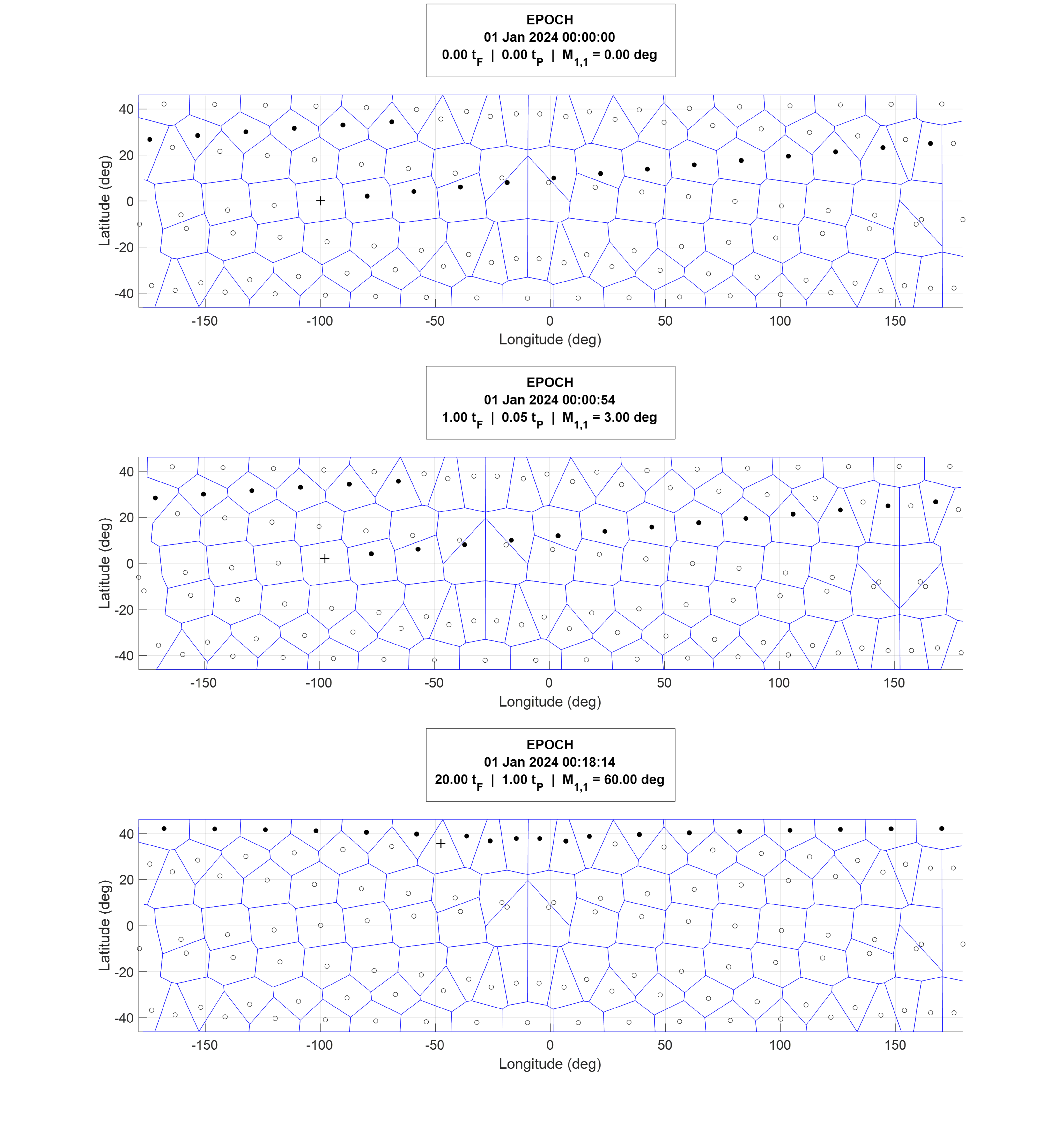
Figure 2: Walker-Delta patterns in geographic coordinate frame at epoch time, $t_{F}$, and $t_{P}$ ($+$: ${SAT}_{1,1}$, $\medbullet$: ${SAT}_{\textbf{M},1}$, $\medcirc$: the rest satellites)

On the other hand, the mean anomaly propagates $P\text{PU}$ during $t_{P}$ and it defines the second pattern repetition period as

$$t_{P}=P\cdot\frac{360}{T}\cdot\frac{1}{\omega_{orb}}\text{sec}$$ (9)

The RAAN and mean anomaly at $t_{P}$ are derived as

$$\Omega_{m}\left(t_{P}\right)=\Omega_{m}\left(t_{0}\right)=S\cdot\left(m-1\right)\text{PU}$$ (10)

$$M_{m,n}\left(t_{P}\right) =F\cdot\left(m-1\right)+P\cdot n\text{PU}$$ (11)

$$=M_{m,n+1}\left(t_{0}\right)$$

Let us define the set of satellites in the $m$th orbital plane as $\textbf{N}=\left\{n\mid n=1,2,...,S\right\}$. Then, the equations (10) and (11) derives

$$M_{m,\textbf{N}}\left(t_{P}\right)=M_{m,\textbf{N}}\left(t_{0}\right).$$ (12)

Therefore, the constellation pattern at $t_{P}$ appears exactly the same as the pattern at $t_{0}$.

Figure 2 is the pattern of Walker-Delta constellation for $i$: $T/P(S)/F$ = $42$: $120/20(6)/1$ in geographic coordinate frame. The marks are subsatellite points and $+$, $\medbullet$, and $\medcirc$ represents ${SAT}_{1,1}$, ${SAT}_{\textbf{M},1}$, and the rest satellites where $\textbf{M}=\left\{m|m=1,2,...,P\right\}$ is the set of orbital plane numbers. The blue line is the bounded Voronoi diagram for the mid latitude and equator region that will be described in the next chapter. The ${SAT}_{1,1}$ barely moved in the middle panel compared to the top panel because $t_{F}$ is only 54 seconds. However, the blue diagrams show that the pattern of the whole constellation is moved westward for $\Delta\Omega=18.00\deg$. The bottom panel is the pattern at $t_{P}$, which is 18 minutes and 14 seconds. The position of each satellite propagated from the epoch time, the top panel, but the patterns of the top and bottom panels are the same.

2.1.2 Duplicate Allocation of Orbital Elements

The Walker-Delta design method allocates the six unique orbital elements to each satellite corresponding to the orbital state of six position and velocity elements. It suggests the possibility of the duplicate positions of the satellites and implies the redundant number of satellites or the collisions between satellites. The conditions of duplicate orbital elements of Walker-Delta constellation is investigated in the reference 4 as

$$\begin{cases}\Omega_{m^{\prime},n^{\prime}}-\Omega_{m,n}=180\deg\\ M_{m^{\prime},n^{\prime}}-M_{m,n}=180\deg.\end{cases}$$ (13)

The equation (13) can be expressed by Walker-Delta design parameters as

$$\begin{cases}m^{\prime}=1+\frac{P}{2}\\ n^{\prime}=1+\frac{S-F}{2}.\end{cases}$$ (14)

In the design procedure, the Walker-Delta design parameters that accommodate the Eq. (14) should be avoided.

2.2 Common Ground-track Constellation

2.2.1 Repeat Ground-track Orbit

The repeat ground-track orbit (RGT) is defined as the orbit that traces the same ground-track within a specified time interval. The two main parameters that determines the RGT orbit are the revolutions to repeat ($N_{P}$) and the days to repeat ($N_{D}$)[5]. For example, if the revolutions to repeat is $14$ and the days to repeat is $1$, the ground-track crosses (ascends or descends) the equator 14 times during 1 day. From this, the period ratio ($\nu$), the RGT design parameter, is formulated as

$$\nu={N_{P}}/{N_{D}}$$ (15)

The period ratio can also be described by the satellite nodal period ($T_{S}$) and the nodal period of greenwich ($T_{G}$). The change of the orbital elements by $J_{2}$ effect induces the changes in $T_{S}$ and $T_{G}$ as

$$T_{S}=\frac{2\pi}{\dot{\omega}+\dot{M}}$$ (16)

$$T_{G}=\frac{2\pi}{\omega_{E}-\dot{\Omega}}$$ (17)

where $\omega$ is the argument of the perigee, $\Omega$ is the right ascension of the ascending node (RAAN), $M$ is the mean anomaly, $\omega_{E}$ is the Earth’s rotation speed.

The orbital elements are formulated as Eqs. (18), (19), and (20)

$$\dot{\omega}=\frac{3}{2}J_{2}\frac{R_{E}}{p}^{2}\sqrt{\frac{\mu_{E}}{a^{3}}}\left(2-\frac{5}{2}\sin{i}^{2}\right)$$ (18)

$$\dot{M}=\sqrt{\frac{\mu_{E}}{a^{3}}}\left(1-\frac{3}{2}J_{2}\left(\frac{R_{E}}{p}\right)^{2}\sqrt{1-e^{2}}\left(\frac{3}{2}\sin{i}^{2}-1\right)\right)$$ (19)

$$\dot{\Omega}=-\frac{3}{2}J_{2}\left(\frac{R_{E}}{p}\right)^{2}\sqrt{\frac{\mu_{E}}{p}^{2}}\cos{i}$$ (20)

From the definition of the period ratio, the introduction of Eqs. (16) and (17) derives the Eq. (15) with respect to the orbital elements.

$$\nu=\frac{N_{P}}{N_{D}}=\frac{T_{G}}{T_{S}}=\frac{\dot{\omega}+\dot{M}}{\omega_{E}-\dot{\Omega}}$$ (21)

From the Eqs. (18), (19), and (20), the orbital elements have their arguments as $\dot{\omega}=\dot{\omega}\left(a,i,e\right)$, $\dot{M}=\dot{M}\left(a,i,e\right)$, and $\dot{\Omega}=\dot{\Omega}\left(a,i,e\right)$. It organizes the arguments of $T_{S}$, $T_{G}$, and $\nu$ as

$$T_{S}=T_{S}\left(a,e,i\right)$$ (22)

$$T_{G}=T_{G}\left(a,e,i\right)$$ (23)

$$\nu=\nu\left(a,e,i\right)$$ (24)

From this, the RGT orbital design algorithm can be derived. Given the specific $\nu$, inclination ($i$), and eccentricity ($e$), the algorithm calculates the corresponding semi-major axis (a). The equation (15) implies that $\nu$ determines the number of revolutions per a certain period and suggests that $\nu$ is related to the orbital period and the semi-major axis. As a result, when $e$ and $i$ are specified, one unique semi-major axis is derived from a $\nu$ and vice versa. For example, if the set of RGt orbital elements is given as $\left(\nu,i,e\right)=\left(14,42\deg,0\right)$, then $a$ is $7201.90km$. The RGT orbital elements can be described in a different way, such as $\left(a,i,e\right)=\left(7201.90km,42\deg,0\right)$, then $\nu$ is uniquely determined as $14$.

2.2.2 Common Ground-track Constellation

The RGT orbit designed following the Eq. (21) has a set of $\left(\nu,i,e\right)$ or $\left(a,i,e\right)$ with an arbitrary set of $\left(\omega,\Omega,M\right)$. From here on, the orbital elements of RGT orbit is described as $\left(\nu,i,e\right)$ except a specific purpose. This implies that a numerous number of satellites could trace the same ground-track and introduces the concept of common ground-track (CGT) constellation. The CGT constellation is designed following the the three procedures below[6, 7]:
(1) Calculate the semi-major axis ($a$) of the seed satellite from $\left(\nu,i,e\right)$ in Eq. (21).
(2) Choose an arbitrary $\omega$ so that all the satellites have the same $\left(\nu,i,e,\omega\right)$.
(3) Given the CGT constellation’s total number of satellite ($T$), the $k$th satellite’s RAAN and mean anomaly $\left(\Omega_{k},M_{k}\right)$ satisfies Eq. (25)

$$N_{P}\Omega_{k}+N_{D}M_{k}=constant\mod{2\pi}$$ (25)

where $k=1,...,T$.

The CGT constellation design problem is concluded as the configuration method of $\left(\Omega_{k},M_{k}\right)$ following the procedure (3). The reference  [7] introduces two methods: the quasi-symmetric and binary integer programming (BILP) method.

2.2.3 Quasi-symmetric Method

The simulation time ($T_{sim}$) is discretized by the step size $t_{step}$ and is assumed to be the integer multiple of the repetition period. Then, it can be formulated as $T_{sim}=L\cdot t_{step}$. The continuous time variable $t\in\left[0,T_{sim}\right]$ is converted into the discretized time variable $\tau\in\left\{0,1,...,L-1\right\}$. The configuration of the satellites of the CGT constellation can be expressed as the time shifted seed satellites because all the satellites have the same ground-track traces. Therefore, the constellation pattern vector $x\left[\tau\right]$ can be defined as

$$x\left[\tau\right]\triangleq\begin{cases}1&\text{if $\tau=\tau_{k}$},\\ 0&\text{otherwise}.\\ \end{cases}$$ (26)

where $\tau_{k}$ is the temporal location of the $k$th satellite.

In the discretized time domain, the constellation pattern vector has the length $L$. If the total number of the constellation is $T$, the spacing constant $\xi$ is defined as

$$\xi\triangleq\frac{L}{T}$$ (27)

.

If $\xi$ is an integer, $\tau_{k}$ is spaced equally and the satellites are configured symmetrically. On the other hand, if $T$ is not a divisor of $L$, then $\xi$ is not an integer that makes the index $\tau_{k}$ also a rational number. In this case, only a quasi-symmetric configuration is possible. The formulation for both symmetric and quasi-symmetric constellation pattern vector $\overline{x}\left[\tau\right]$ is defined as

$$\overline{x}\left[\tau\right]\triangleq\sum_{k=1}^{T}\delta\left[nint\left(\tau-\xi\left(k-1\right)\right)\right]$$ (28)

where $nint$ is the nearest integer function.

2.2.4 Binary Integer Linear Programming Method

Because the domain of the constellation pattern vector is defined as binary, BILP method is introduced as the optimization algorithm. The BILP algorithm is one of the variants of the linear programming method that optimizes the linearized objective function with the constraints and boundaries. The problem statement of the linear programming can be generalized as[8]

$$\min_{x}{\textbf{{c}}^{T}\textbf{{x}}}\text{ subject to}\begin{cases}\textbf{A}\cdot\textbf{{x}}\leq\textbf{{b}}\\ \textbf{A}_{eq}\cdot\textbf{{x}}=\textbf{{b}}_{eq}\end{cases}$$ (29)

where x is the decision variable of length $L$, $\textbf{{c}}^{T}\textbf{{x}}$ is the objective function, $\textbf{A}\in\mathbb{R}^{Q\times L}$ and $\textbf{{b}}\in\mathbb{R}^{Q}$ are the matrix and vector that constitutes the $Q$ numbers of inequality constraints, $\textbf{A}_{eq}\in\mathbb{R}^{R\times L}$ and $\textbf{{b}}\in\mathbb{R}^{R}$ are the matrix and vector of $R$ numbers of equality constraints.

In addition to Eq. (29), the domain of the decision variable x needs to be defined. The domain sets of $\mathbb{R}_{\geq 0}$, $\mathbb{Z}_{\geq 0}$, and $\mathbb{Z}_{2}$ induce the pure real, integer, and binary integer linear programming. The mixed domains are also possible that mixed integer linear programming have the real and integer decision variables. Thus, the BILP has the same problem statement but constraints the domain of decision variables as

$$\textbf{{x}}\in\mathbb{Z}_{2}^{L}$$ (30)

The objective of the optimization is to obtain the constellation pattern vector that minimizes the number of satellites while satisfying the coverage requirement. Since the summation of $x\left[\tau\right]$ is equal to $T$ by the definition of the constellation pattern vector in Eq. (26), the problem is formulated as

$$\min_{x}{\textbf{{1}}}^{T}\textbf{{x}}\text{ subject to}\begin{cases}\textbf{V}_{0,j}\textbf{{x}}\geq\textbf{{f}}_{j},&\forall j\in\mathcal{J}\\ \textbf{{x}}\in\mathbb{Z}_{2}^{L}\end{cases}$$ (31)

where $j$ is the index for the $j$th grid, $\mathcal{J}$ is the set of grids in the area of interest and $\mathbb{Z}_{2}$ is the binary integer number set. The matrix $\textbf{V}_{0,j}\in\mathbb{Z}_{2}^{L\times L}$ is a seed-satellite access profile circulant matrix and will be addressed in detail in the next chapter.

3 Coverage Analysis Methods

3.1 Geometry of Earth Coverage

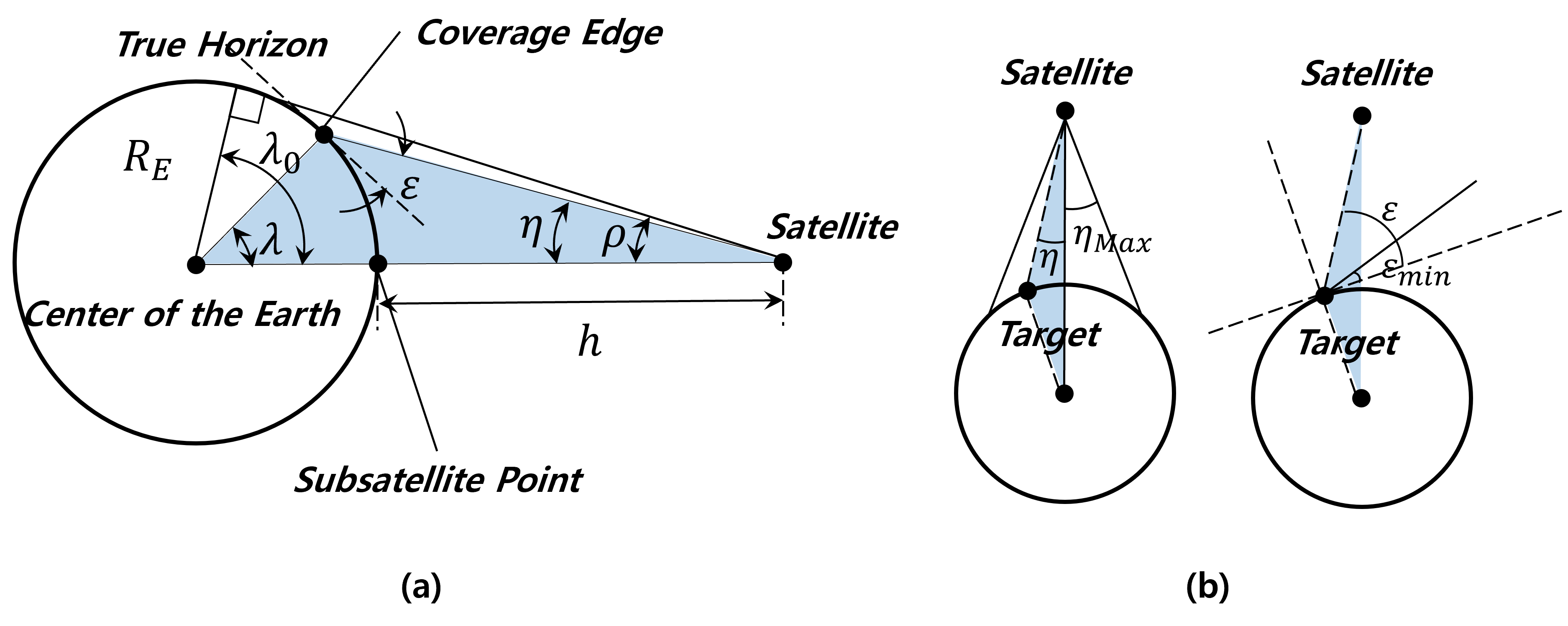
Figure 3: (a) Geometric relationships between the satellite, coverage edge, and center of the Earth and (b) geometric description of coverage

Figure 3a describes the geometric relationships between the satellite, coverage edge, and center of the Earth are advantageous for coverage analysis. The true horizon is tangent from the satellite to the Earth’s surface. The angle between the true horizon and the subsatellite point is called the maximum Earth central angle (ECA, $\lambda_{0}$) or the angular radius of the Earth ($\rho$) when measured from the center of the Earth and the satellite, respectively. When the satellite is located at an altitude of h km, the angular radius of the Earth is determined by Eq. (32), where $R_{E}$ is the Earth’s radius.

$$\sin{\rho}=\frac{R_{E}}{R_{E}+h}$$ (32)

Usually, the payload’s coverage determines the coverage performance of a single satellite that constitutes the constellation. The Earth central angle ($\lambda$) measures the size of the payload’s coverage ($\eta$) on the surface of the Earth and is defined as the angular distance between the subsatellite point (SSP) and the coverage edge. The coverage edge is the rim of the satellite’s coverage on Earth. The elevation angle ($\varepsilon$) is measured at the coverage edge from the local horizontal to the satellite.

The coverage can be approached from two perspectives: the satellite and the target area (Figure 3b). When considering the satellite perspective, it’s important to evaluate the payload’s specification. According to the definition of the coverage, the nadir angle ($\eta=\eta(t)$) should be smaller than the payload’s beam coverage ($\eta_{Max}$). From the target point perspective, it is considered as covered when the elevation angle of the satellite ($\varepsilon=\varepsilon(t)$) is greater than the target point’s minimum elevation angle ($\varepsilon_{min}$).

The trigonometry of the blue shaded triangle in Figure 3a derives the formulae between $\eta$, $\varepsilon$, and $\lambda$ as Eqs. (33) and (34).

$$\cos{\varepsilon}=\sin{\eta}/\sin{\rho}$$ (33)

$$\lambda=90\deg-\eta-\varepsilon$$ (34)

For the communication constellations, the constraints are imposed on both the payload specification and the elevation angle of the target point. Therefore, the trigonometry in Eqs. (33) and (34) is crucial as it prevents redundant computational complexity. For example, suppose that the beam coverage of the spacecraft ($\eta_{Max}$) is $45$ deg and the ground station has a minimum elevation angle ($\varepsilon_{min}$) of $30$ deg. If the satellite’s altitude is $1,200$ km, the angular radius of the Earth ($\rho$) is $57.31$ deg. The Eq. (33) immediately converts the payload’s coverage to the elevation angle as

$$\overline{\varepsilon}=\arccos{\left(\sin{\eta_{Max}}/\sin{\rho}\right)}=32.84\deg$$ (35)

where $\overline{\varepsilon}$ is the elevation angle that corresponds to $\eta_{Max}$ and does not have a physical meaning. The ECA ($\overline{\lambda}$) is calculated from Eq. (34) as

$$\overline{\lambda}=90-\eta_{Max}-\overline{\varepsilon}=12.16\deg$$ (36)

In the same manner, the minimum elevation angle ($\varepsilon_{min}$) derives its corresponding parameters as $\tilde{\eta}=46.79$ deg and $\tilde{\lambda}=13.21$ deg. The ECA is the visualized size of the coverage on the Earth’s surface and the smaller the ECA is, the more degraded the coverage performance is. Therefore, the simulation only with $\overline{\lambda}$, $\eta_{Max}$, or $\overline{\varepsilon}$ is enough to analyze if the constellation satisfies the coverage requirement. Since the coverage analyses with $\overline{\lambda}$, $\eta_{Max}$, or $\overline{\varepsilon}$ show the same results but only conducted at different perspectives, the simulation with only one of three constraints reduces the computational cost.

3.2 Voronoi Tessellation

The problem of continuous coverage constellation can be reduced to obtaining the circumradius of the adjacent three points. For a set of discretized points, the circumradius of the adjacent three points can be defined. When the circumradius is less than a specified value, the distance from any point within the region is shorter than the specified value. References 2 and 3 introduced the satellite triad method as the coverage analysis technique for the Walker constellation. The research subject of the references was the constellation of less than 20 satellites. This research utilizes the Delaunay triangulation method that is first suggested in the reference 4 to generalize the number of satellites of the constellation.

The Delaunay triangulation is a computational geometry subdividing the discretized points into triangles[9]. This algorithm defines the Delaunay criterion to construct the Delaunay conformant triangles that do not contain other points inside the circumcircles. The Voronoi diagram (VD) is the dual graph of the Delaunay triangle (DT) and is drawn by connecting the circumcenters of the Delaunay triangles. The Voronoi tessellation is the tiling of a plane or a sphere with Voronoi diagrams. If the tiled region is a restricted closed area on the sphere, the Voronoi diagrams have boundaries cut by the boundary and are called bounded Voronoi diagram (BVD) [10, 4]. The constellation coverage problem can be formulated as the Voronoi tessellation problem. The subsatellite points on the Earth’s surface are the discretized points on the three-dimensional spherical surface. The area of interest is not the whole globe, the Voronoi diagram is bounded within the target region. The spherical Delaunay triangles and spherical bounded Voronoi diagram will derive the solution, but the word ’spherical’ will be omitted for brevity from here on.

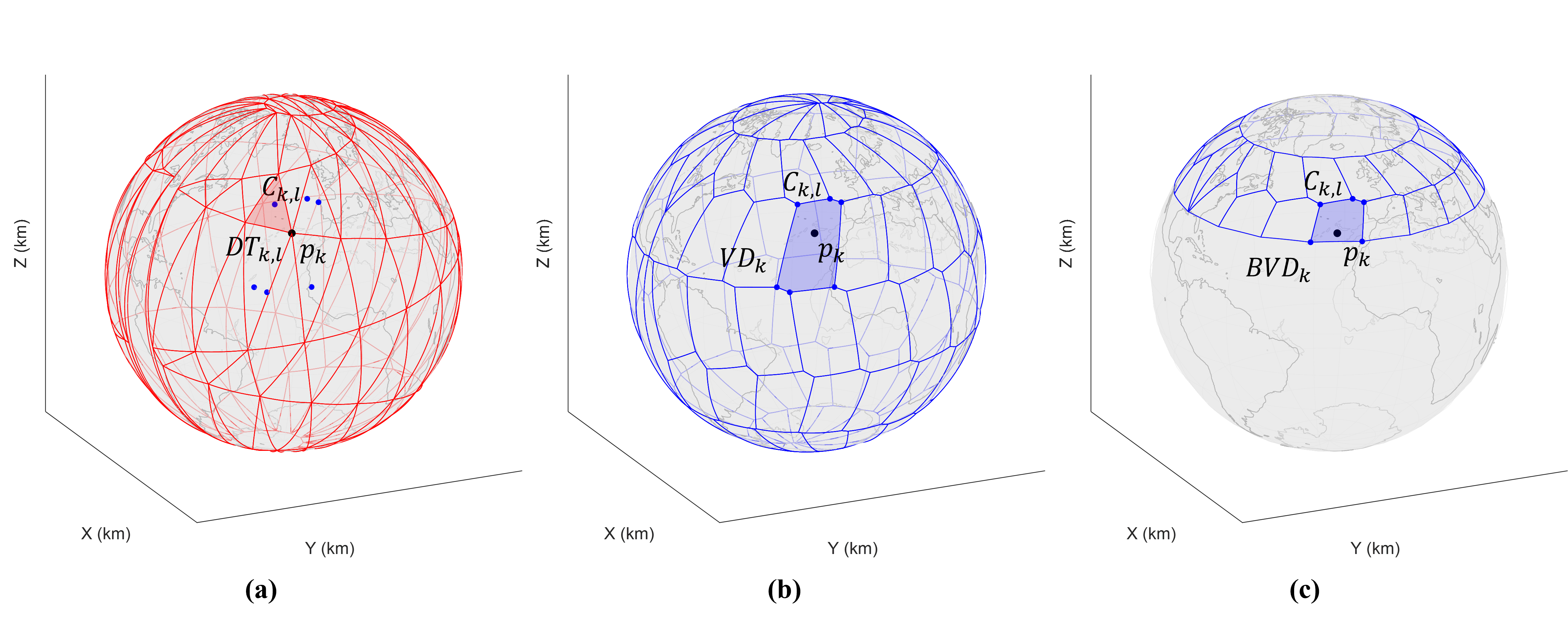
Figure 4: Example: (a) Delaunay triangle, (b) Voronoi diagram, and (c) Bounded Voronoi diagram

Figure 4 depicts an example of the Delaunay triangle, Voronoi diagram, and the bounded Voronoi diagram. In Figure 4(a), there are six DTs that contains $p_{k}$ as their vertices for an arbitrary subsatellite point $p_{k}$, where $k=1,2,...,T$. The ${DT}_{k,l}$ are depicted as red triangles, and the circumcenters $C_{k,l}$ are blue dots, where $l=1,2,...,N_{k}$. The $N_{k}$ is the number of triangles that have the vertice $p_{k}$, and can be different for each $p_{k}$. Any subsatellite point posseses only one VD, and the $VD_{k}$ is drawn by connecting the blue dots, the circumcenters $\textbf{C}_{k}=\left\{C_{k,l}\mid l=1,2,...,N_{k}\right\}$, as in Figure 4(b).

The Voronoi diagram in Figure 4(b) can be utilized for the global coverage problem. However, for the regional coverage problem, the Voronoi diagram should be bounded within the area of interest. Especially, for the regional continuous coverage problem, the Voronoi diagram bounded within the latitude range of AoI as a circular band can efficiently analyze the continuity of the constellation[4]. Suppose that the northern area of interest, then the bounded Voronoi diagram appears Figure 4(c). Then, $p_{k}$ has ${BVD}_{k}$ with different vertices $\overline{\textbf{C}}_{k}=\left\{\overline{C}_{k,\overline{l}}\mid\overline{l}=1,2,...,\overline{N}_{k}\right\}$.

Let us define the angular distance $\theta_{k,\overline{l}}$ as the angular distance between the subsatellite point $p_{k}$ and the vertices $\overline{C}_{k,\overline{l}}$. Then, the maximum distance of the ${BVD}_{k}$ of the $k$th satellite is expressed as

$$\theta_{max,k}=\max_{\overline{l}}{\theta_{k,\overline{l}}}$$ (37)

As a result, the maximum angular distance of the whole constellation is obtained as

$$\theta_{max}=\max_{k}{\theta_{max,k}}$$ (38)

Assuming the homogeneous constellation, the coverage performances of all the satellites are the same and can be expressed as $\lambda^{*}$. Then, the continuous coverage problem statement is defined as

$$\theta_{max}\leq\lambda^{*}.$$ (39)

For the global coverage problem, the maximum angular distance should be defined from $\theta_{k,l}$ and $C_{k,l}$, and the rest procedures are the same.

3.3 APC Decomposition

The reference 7 developed the APC decomposition from the circular convolution phenomenon between a seed satellite’s access profile, a constellation pattern vector, and a coverage timeline. The access profile between the $k$th satellite and the $j$th target point ($\textbf{{v}}_{k,j}$) defines its elements as

$$v_{k,j}\left[\tau\right]\triangleq\begin{cases}1&\text{if $\varepsilon_{k,j}\left[\tau\right]\geq\varepsilon_{k,j,min}\left[\tau\right]$ }\\ 0&\text{otherwise}\end{cases}$$ (40)

where $\tau$ is the discretized time variable, and $\mathcal{J}$ is the set of target points.

The coverage timeline of the constellation $\textbf{{b}}_{j}$ is derived as the summation of all the access profiles:

$$b_{j}\left[\tau\right]=\sum_{k=1}^{T}{v_{k,j}}\left[\tau\right]$$ (41)

The circular convolution phenomenon expresses the coverage timeline $\textbf{{b}}_{j}$ with respect to the seed-satellite access profile $\textbf{{v}}_{0,j}$ and the coverage pattern vector x as

$$b_{j}\left[\tau\right]=v_{0,j}\left[\tau\right]\circledast x\left[\tau\right]$$ (42)

where x is defined in Eq. (25) and $\circledast$ is the circular convolution operator.

This circular convolution operation can be described in a linearized form as

$$\textbf{{b}}_{j}=\textbf{V}_{0,j}\textbf{{x}}$$ (43)

where $\textbf{V}_{0,j}$ is the matrix in Eq. (31).

In summary, the coverage timeline of the whole constellation is obtained from the circular convolution of the seed-satellite access profile and the constellation pattern vector. This concept of APC decomposition reduces the optimal CGT constellation design problem to the constellation pattern vector optimization problem.

4 Relative Motion in Adjacent Orbital Planes

The satellites in the adjacent orbital planes ${SAT}_{m,n}$ and ${SAT}_{m+1,n}$ have the angular distances in terms of the differential RAAN and mean anomaly as

$$\Delta u=M_{m+1,n}-M_{m,n}=\frac{360}{T}\cdot F\deg$$ (44)

$$\Delta\Omega=\Omega_{m+1,n}-\Omega_{m,n}=\frac{360}{P}\deg$$ (45)

Since the Walker-Delta constellation satellites are designed to have the same altitude and inclination, the relative motion between ${SAT}_{m+1,n}$ and ${SAT}_{m,n}$ can be described analytically [11]. The minimum and maximum relative angular distances ($\theta_{min}$ and $\theta_{max}$) are formulated as

$$\sin{\left(\theta_{min}/2\right)}=\sin{\left(\phi_{R}/2\right)}\cos{\left(i_{R}/2\right)}$$ (46)

$$\cos{\left(\theta_{max}/2\right)}=\cos{\left(\phi_{R}/2\right)}\cos{\left(i_{R}/2\right)}$$ (47)

where $i_{R}$ is the relative inclination and $\phi_{R}$ is the relative phase.

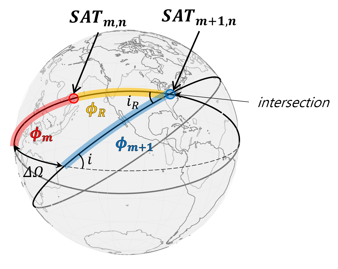
Figure 5: Relative motion of the satellites in the adjacent orbital planes

The relative inclination $i_{R}$ in Figure 5 is the angle between the orbital planes measured at the orbital intersection and is derived from spherical trigonometry as

$$\cos{i_{R}}=\cos{i}^{2}+\sin{i}^{2}\cos{\Delta\Omega}$$ (48)

$$\rightarrow i_{R}=i_{R}\left(i;P\right)$$

where Eq. (45) is used.

The spherical triangle in Figure 5 derives the geometric relationship between the relative phase $\phi_{R}$ and angular distances $\phi_{m}$ and $\phi_{m+1}$ as

$$\phi_{m}+\phi_{R}-\phi_{m+1}=180-2\phi_{m+1}$$ (49)

where the spherical trigonometric rule that the differential arc between the intersected orbits is $180-2\phi_{m+1}$ is used. The relative phase $\phi_{R}$ is obtained by reorganizing Eq. (49)

$$\phi_{R} =180-2\phi_{m+1}+\left(\phi_{m+1}-\phi_{m}\right)$$ (50)

$$=180-2\phi_{m+1}+\Delta u$$

where the differential angular distance $\phi_{m+1}-\phi_{m}$ is the relative argument of latitude $\Delta u$ in the Walker-Delta constellation. The formula to calculate $\phi_{m+1}$ is as follows:

$$\tan{\phi_{m+1}}=\frac{\tan{\left(90-\Delta\Omega/2\right)}}{\cos{i}}$$ (51)

$$\rightarrow\phi_{m+1}=\phi_{m+1}\left(i;P\right)$$

As a result, Eq. (51) provides the argument of $\phi_{R}$ as

$$\phi_{R}=\phi_{R}\left(i;T,P,F\right)$$ (52)

The inter-satellite link (ISL) constraints the range of relative motion so that the signal is not interfered within the link margin. Therefore, the minimum and maximum relative distances in Eqs. (46) and (47) contained within the specified range could guarantee smooth ISL communication.

The relative motion in the adjacent orbital plane described in Eqs. (48), (50), and (51) explains the relative motion between ${SAT}_{m,n}$ and ${SAT}_{m+1,n}$ where $m=1,...,P-1$ and $n=1,...,S$. When $m=P$, the relative motion between ${SAT}_{P,n}$ and ${SAT}_{1,n+F}$ is proven the same with the one between ${SAT}_{m,n}$ and ${SAT}_{m+1,n}$ by Eqs. (1), (2), (48), (50) and (51). As a result, if Eqs. (46) and (47) satisfy the constraint on the ISL link, then all the ISL links are connected without any isolated link.

5 Simulation Results

5.1 Continuous Coverage Analysis

The constellation is designed with the three constellation design methods introduced in the previous sections: Walker-Delta constellation, Quasi-symmetric CGT constellation, and BILP CGT constellation. The seed satellite for the three constellations is designed to have the repetition period $\nu=14/1$. The inclination is 42 degrees which is 3–5 degrees higher than the area of interest[12, 13]. The minimum elevation angle $\varepsilon_{min}$ is 15 degrees and the target point is located at Seoul. The Walker-Delta constellation is analyzed assuming two-body motion and the target area is the circle of radius 100 km around Seoul. The CGT constellations assume $J_{2}$ perturbation and a single target point. The sampling time or time step $t_{step}$ is 1 and 300 seconds for Walker-Delta and CGT constellations respectively, and the simulation time horizon is 1 day for both.

5.1.1 Walker-Delta Constellation

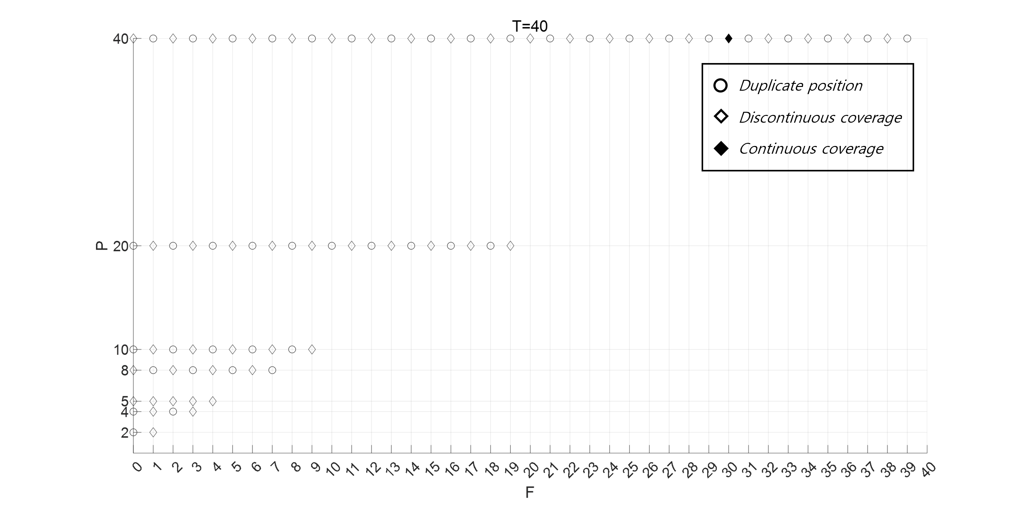
Figure 6: Bounded Voronoi diagram result of Walker-Delta constellation ($i$: $T$ = 42: 40)

Figure 6 depicts the bounded Voronoi diagram simulation result of Walker-Delta constellation. The global search from the less number of satellites obtains that 40 satellites at the inclination 42 $\deg$ is the minimum number of satellites to achieve the continuous coverage by Walker-Delta constellation. The empty circles are the $T/P/F$ parameters that have duplicate positions in Eq. (14) and are preclude from coverage analysis. The empty diamond markers mean that the parameters could not achieve continuous coverage. The continuous coverage solution is $i$: $T/P(S)/F$ = $42$: $40/40(1)/30$ and denoted as the black diamond. The ECA of this solution ($\lambda^{*}$) is $15.86\deg$.

5.1.2 Common Ground-track Constellations

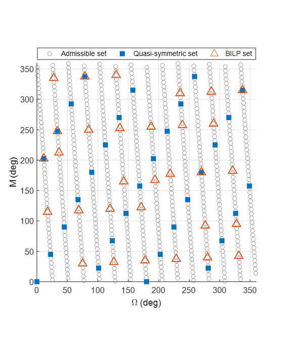
Figure 7: Configurations of quasi-symmetric and BILP CGT constellations in ($\Omega,M$) space

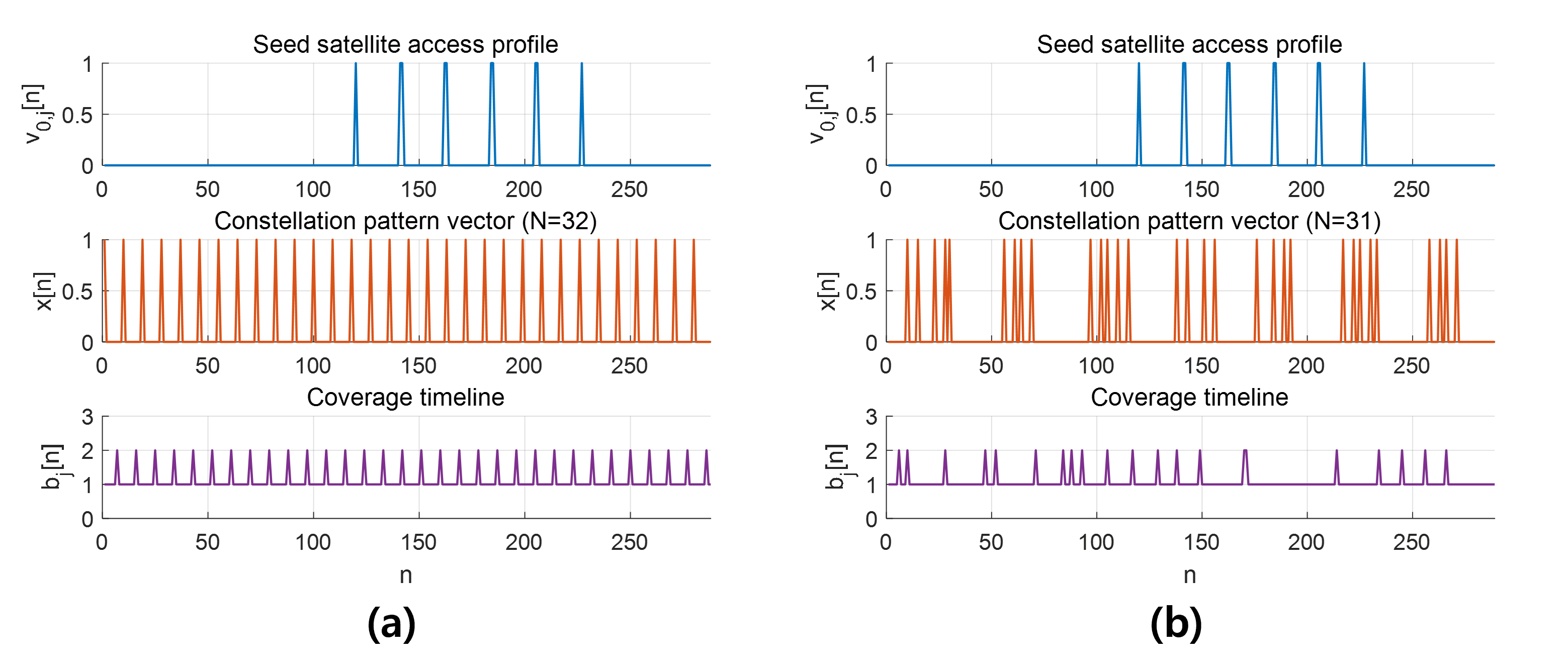
Figure 8: APC Decomposition of (a) quasi-symmetric and (b) BILP CGT constellation

The quasi-symmetric constellation pattern vector $x_{qs}$ and BILP constellation pattern vector $x_{bilp}$ are obtained as

$$x_{qs}=\begin{cases}1&\text{for }n=\{0,9,18,27,36,45,54,63,72,81,90,99,108,117,126,135,...\\ &144,153,162,171,180,189,198,207,216,225,234,243,252,261,270,279\}\\ 0&\text{otherwise}\end{cases}$$ (53)

$$x_{bilp}=\begin{cases}1&\text{for }n=\{9,14,22,27,29,55,60,63,68,96,101,104,109,114,137,...\\ &142,150,155,175,183,188,191,216,221,224,229,232,257,262,265,270\}\\ 0&\text{otherwise}\end{cases}$$ (54)

The CGT constellation’s pattern reveals its characteristics in the $\left(\Omega,M\right)$ space such as the period ratio and symmetricity (Figure 7). The gradient of admissible set is $-N_{P}/N_{D}$ and equal to $-\nu$ by Eqs. (25) and (15). The constellation pattern vectors are laid on some points along the admissible set. The quasi-symmetric set configures symmetrically in Figure 7 as $\textbf{{x}}_{qs}$ on the second panel of Figure 8a is equally spaced. Because the $N_{qs}$ is 32 and $L$ is 288, $L/N_{qs}$ is divided as the integer 9 and the spacing is perfectly symmetric. On the other hand, the BILP constellation pattern vector is irregularly spaced in Figures 7 and 8b. However, the BILP constellation achieves less number of satellites $N_{bilp}$ as 31 while both constellations exhibit the single-fold coverage.

5.2 Inter-satellite Link Continuity Analysis

5.2.1 Walker-Delta Constellation

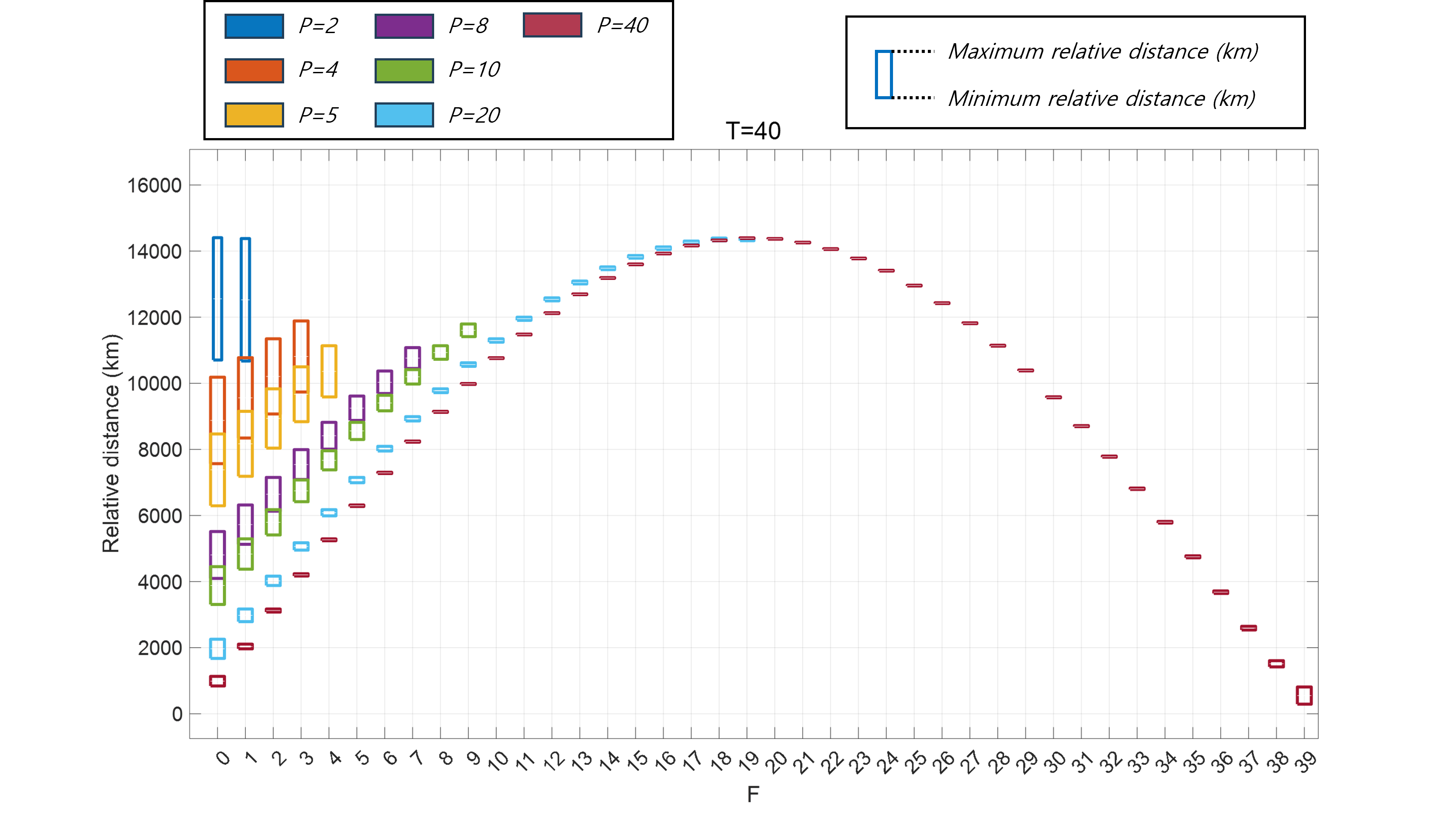
Figure 9: Relative motion between the adjacent orbital plane of Walker-Delta constellation ($i$: $T$ = 42: 40)

The minimum and maximum relative distances are the line distance calculated from the angular distances in Eqs. (46) and (47) (Figure 9). The upper and lower bound of bars reveal the relative distance ranges in the adjacent orbital planes. The color of the bars distinguish the number of planes and the x axis is $F$ numbers. Since this graph shows the relative motion at a glance, it is a useful tool for ISL connectivity analysis. The continuous coverage solution $i$: $T/P(S)/F$ = $42$: $40/40(1)/30$ has the relative motion range from $9559.77km$ to $9589.64km$.

5.2.2 Common Ground-track Constellation

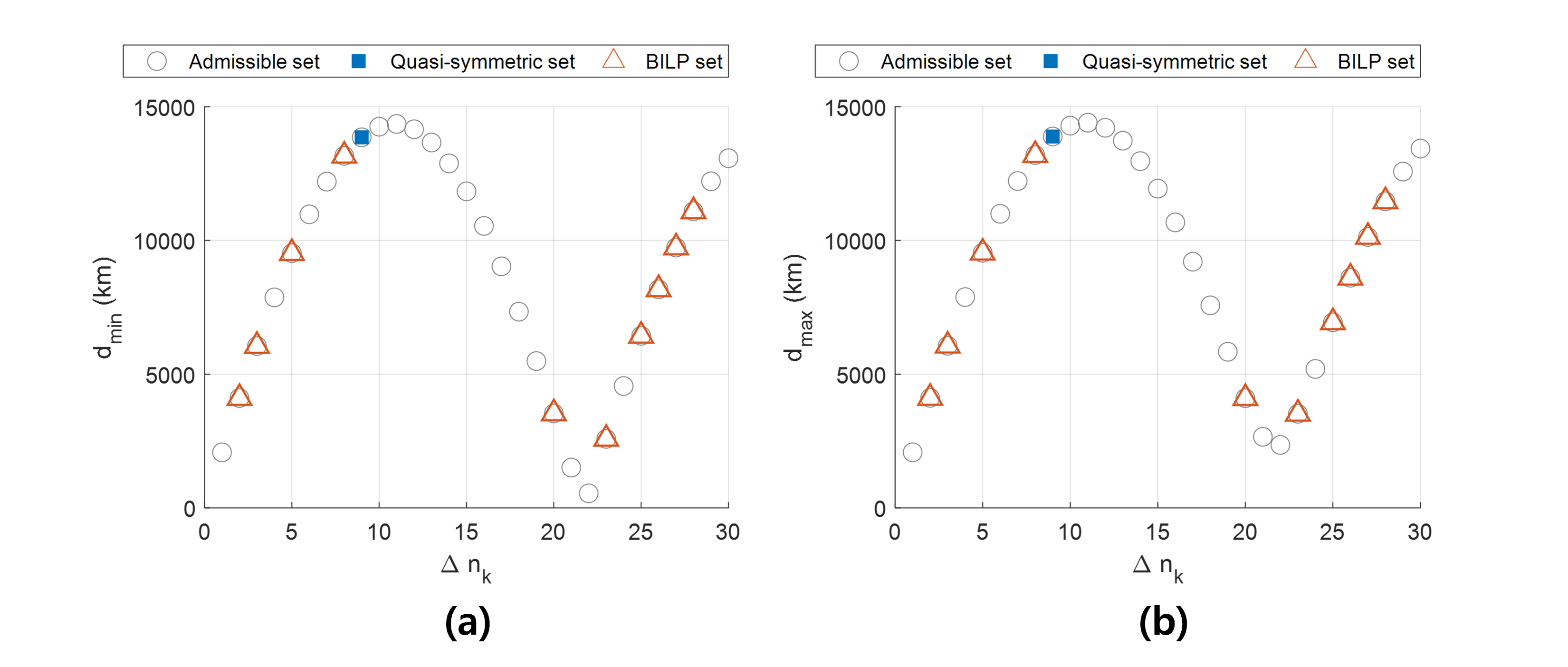
Figure 10: (a) Minimum and (b) maximum relative distance between the adjacent orbital plane of quasi-symmetric and BILP CGT constellations

The relative motion equations (48), (50), and (51) implies that the relative motion of two orbits with the same altitude and inclination is the function of the inclination, relative RAAN, and relative argument of latitude. Let us define the set of temporal location $\tau_{k}$ in Eq. (26) as $\boldsymbol{\tau}_{k}$, then $\boldsymbol{\tau}_{k,qs}$ and $\boldsymbol{\tau}_{k,bilp}$ are calculated as Eqs. (53) and (54). The temporal location $\tau_{k}$ derives the RAAN $\Omega_{k}$ as Eq. (55)[7].

$$\Omega_{k}=\tau_{k}\cdot\frac{2\pi N_{D}}{L}+\Omega_{0}$$ (55)

where the subscript ’0’ means the variable is relevant to the seed satellite. The equation (25) describes the relationship between $\Omega_{k}$ obtains $M_{k}$.

Let us define $\Delta\tau_{k}$, the subtraction of the consecutive $\tau_{k}$, as

$$\Delta\tau_{k}=\begin{cases}\tau_{k+1}-\tau_{k}&\text{for $k=1,...,T-1$}\\ \tau_{k}+L-\tau_{1}&\text{for $k=T$}\end{cases}$$ (56)

Thus, the equations (53), (54), and (56) calculates $\Delta\tau_{k}$ for the two CGT constellations as

$$\Delta\tau_{k,qs}=9$$ (57)

$$\Delta\tau_{k,bilp}=2,3,5,8,20,23,25,26,27,28$$ (58)

The equation (55) derives the relative RAAN $\Delta\Omega_{k}$ and relative mean anomaly $\Delta M_{k}$ as

$$\begin{cases}\Delta\Omega_{k,qs}=11.25\deg\\ \Delta M_{k,qs}=202.50\deg\end{cases}$$ (59)

$$\begin{cases}\Delta\Omega_{k,bilp}=2.5,3.75,6.25,10.00,25.00,28.75,31.25,32.50,33.75,35.00\deg\\ \Delta M_{k,bilp}=10.00,220.00,230.00,247.50,265.00,272.50,282.50,307.50,...\\ \indent\indent\indent\indent\indent 317.50,325.00\deg\end{cases}$$ (60)

The minimum and maximum relative distances in Eqs. (46) and (47) are depicted in Figure 10. The left and right panels appear almost the same because the subtraction between the minimum and maximum distances are less than 1000 km. The minimum and maximum distances for the quasi-symmetric CGT constellation are 13854.32 and 13886.49 km, respectively. The BILP CGT constellation have a variety of $\Delta\tau_{k}$. When $\Delta\tau_{k}$ is 8, the minimum and maximum distances are 13164.56 and 13191.33 km.

6 Conclusion

This paper investigates the continuous coverage analysis methods and inter-satellite link connectivity analysis methods for the communication satellite constellation. The bounded Voronoi diagram designs the homogeneous constellation to have continuous coverage for regional or global coverage. The APC decomposition can be implemented for the CGT constellation’s coverage analysis. The relative motion in the adjacent orbital planes derives the analytic solutions that should be constrained within the inter-satellite link range. The Walker-Delta constellation and two types of CGT constellations are applied as examples. As a result, Walker-Delta constellation design method consists of more satellites than CGT constellations for single-fold coverage. However, the relative motion range is shorter and more consistent, which implies that the Walker-Delta constellation has advantages for inter-satellite links. The quasi-symmetric and BILP methods are suggested for the CGT constellation design method. The BILP optimal CGT constellation has an asymmetric configuration but achieves less number of satellites. The relative motion for BILP constellation have a variety of ranges due to its asymmetricity, but satellites are located closer than the quasi-symmetric constellation. In summary, the BILP constellation is advantageous for the required number of satellites for single-fold coverage. However, the Walker-Delta constellation may have a shorter and more rigorous relative motion range that is beneficial for inter-satellite links.

7 Acknowledgment

Any acknowledgments by the author may appear here. The acknowledgments section is optional. This work was supported by Korea Research Institute for defense Technology planning and advancement (KRIT) grant funded by the Korea government (DAPA (Defense Acquisition Program Administration)) (KRIT-CT-22-040, Heterogeneous Satellite constellation based ISR Research Center, 2024).

8 Notation

$a$	semi-major axis
b	coverage timeline
$e$	eccentricity
f	coverage requirement vector
$i$	inclination
f	coverage requirement
$h$	altitude
$j$	index for grid point
$J_{2}$	coefficient for J2 perturbation
$\mathcal{J}$	set of grid points
$k$	index for satellites
$L$	number of discrete times (length of discrete time variable)
$m$	index for orbital planes
$n$	index for satellites on a plane
$N_{P}$	revolutions to repeat
$N_{D}$	days to repeat
$P$	number of orbital planes
$F$	Phasing parameter
$R_{E}$	Earth radius
$p$	semilatus rectum
$\mu_{E}$	standard gravitational parameter of Earth
$S$	number of satellites on an orbital plane
$T$	total number of satellites
$T_{r}$	repetition period of RGT orbit
$T_{S}$	nodal period of the satellite
$T_{G}$	nodal period of greenwich
$T_{sim}$	simulation time
$t_{step}$	time step
$t$	continuous time variable
$t_{0}$	epoch time
$t_{F}$, $t_{P}$	Walker-Delta pattern repetition period
$u$	argument of latitude
v	access profile
V	access profile circulant matrix
x	constellation pattern vector
$\mathbb{Z}_{2}$	binary integer number set
$\epsilon$	elevation angle
$\eta$	angular size of payload’s coverage
$\rho$	angular radius of Earth
$\lambda$	Earth central angle
$\nu$	period ratio
$\phi$	phase angle
$\tau$	discretized time variable
$\omega$	argument of perigee
$\omega_{E}$	Earth rotation speed
$\omega_{orb}$	orbital angular speed
$\Omega$	right ascension of ascending node
$\xi$	spacing constant
$\theta$	angular distance

References

- [1] I. d. Portillo, B. G. Cameron, and E. F. Crawley, “A technical comparison of three low earth orbit satellite constellation system to provide global broadband,” Acta Astronautica, Vol. 159, 2019, pp. 123–135.
- [2] J. G. Walker, “Circular Orbit Patterns Providing Continuous Whole Earth Coverage,” Technical rept., 1970, pp. 19–23.
- [3] J. G. Walker, “Continuous Whole-Earth Coverage by Circular-Orbit Satellite Patterns,” Technical rept., 1977, pp. 3–26.
- [4] S. Jeon, S.-Y. Park, K. H. Lee, and K.-S. Jeong, “Communication Satellite Constellation Design of Minimum Number of Satellites: Analytic Approach to Walker-Delta Pattern Design,” Journal of the Korean Society for Aeronautical and Space Sciences, Vol. 52, No. 9, 2024, pp. 749–760.
- [5] D. A. Vallado, Fundamentals of Astrodynamics and Applications. Microcosm and Springer, 2013.
- [6] M. E. Avendaño, J. J. Davis, and D. Mortari, “The 2-D Lattice Theory of Flower Constellations,” Celestial Mechanics and Dynamical Astronomy, Vol. 116, No. 4, pp. 325––337.
- [7] H. W. Lee, S. Shimizu, S. Yoshikawa, and K. Ho, “Satellite Constellation Pattern Optimization for Complex Regional Coverage,” Journal of Spacecraft and Rockets, Vol. 57, No. 6, 2020, pp. 1309–1327.
- [8] M. Conforti, G. Cornueljols, and G. Zambelli, Integer Programming. 2014.
- [9] D. Boris, “Sur la sphere vide,” Bulletin de l’Académie des Sciences de l’URSS, Classe des Sciences Mathématiques et Naturelles, Vol. 6, pp. 793–800.
- [10] G. Dai, X. Chen, M. Wang, E. Fernandez, T. N. Nguyen, and G. Reinelt, “Analysis of Satellite Constellations for the Continuous Coverage of Ground Regions,” Journal of Spacecraft and Rockets, Vol. 54, No. 6, 2017, pp. 1294–1303.
- [11] J. R. Wertz, Orbit and constellation design and management. Springer, NewYork, 2009.
- [12] J. R. Wertz, “Coverage, Responsiveness, and Accessibility for Various ’Responsive Orbits’,” 3rd Responsive Space Conference, 2005.
- [13] X. Fu, W. Meiping, and T. Yi, “Design and Maintenance of Low-Earth Repeat-Groundtrack Successive-Coverage Orbits,” Journal of Guidance, Control, and Dynamics, Vol. 35, No. 2, 2012, pp. 686–691.