Ionic association and Wien effect in 2D confined electrolytes

Abstract

Recent experimental advances in nanofluidics have allowed to explore ion transport across molecular-scale pores, in particular for iontronic applications. Two dimensional nanochannels – in which a single molecular layer of electrolyte is confined between solid walls – constitute a unique platform to investigate fluid and ion transport in extreme confinement, highlighting unconventional transport properties. In this work, we study ionic association in 2D nanochannels, and its consequences on non-linear ionic transport, using both molecular dynamics simulations and analytical theory. We show that under sufficient confinement, ions assemble into pairs or larger clusters in a process analogous to a Kosterlitz-Thouless transition, here modified by the dielectric confinement. We further show that the breaking of pairs results in an electric-field dependent conduction, a mechanism usually known as the second Wien effect. However the 2D nature of the system results in non-universal, temperature-dependent, scaling of the conductivity with electric field, leading to ionic coulomb blockade in some regimes. A 2D generalization of the Onsager theory fully accounts for the non-linear transport. These results suggest ways to exploit electrostatic interactions between ions to build new nanofluidic devices.

Introduction

Recent years have witnessed critical advances in the fabrication of atomic-scale fluidic channelsBocquet and Charlaix (2010); Garaj et al. (2010); Lee et al. (2010); Feng et al. (2016); Secchi et al. (2016); Radha et al. (2016); Esfandiar et al. (2017), in an effort to achieve molecular control over water and ion transport – similar to the transport machinery of cells. Considering the intense complexity of such nano-fabrication techniques, theoretical guidance has become necessary; however, traditional continuous models of fluid and charge transport breakdown under such extreme confinementBocquet and Charlaix (2010); Kavokine, Netz, and Bocquet (2021); Kavokine et al. (2019); Kavokine, Robin, and Bocquet (2022); Robin and Bocquet (2023); Richards et al. (2012); Robin et al. (2022); Robin, Kavokine, and Bocquet (2021).

Particular attention has been drawn to 2D nanochannels recentlyRadha et al. (2016); Emmerich et al. (2022) (Figure 1(a)). These systems, which are fabricated by van der Waals assembly, consist in flakes of a 2D material (graphene, MoS₂, hBN…) separated by graphene ribbons, creating an atomically-smooth and -thin channel permeable to water. Electrolytes confined inside such structures are expected to form a single ionic layer, which has been shown to enhance electrostatic interactions between ionsKavokine, Robin, and Bocquet (2022); Robin, Kavokine, and Bocquet (2021) and promote memory effects in conduction, such as the recently-demonstrated memristor effectRobin et al. (2022); Robin, Kavokine, and Bocquet (2021).

The properties of ions in such systems have been studied using various techniques, both in theory – mean field approachesRobin, Kavokine, and Bocquet (2021); Levin (2002), exact field theoriesMinnhagen (1987); Robin et al. (2023)) –, and in simulations – BrownianRobin, Kavokine, and Bocquet (2021); Kavokine, Robin, and Bocquet (2022), molecularRobin, Kavokine, and Bocquet (2021); Zhao et al. (2021) or ab initio dynamicsZhao et al. (2021), and more recently machine learning forcefields trained with DFT-generated datasetsFong et al. (2024). Overall, a growing body of evidence is shedding light on links between electrostatic correlations and non-linear ion transport Avni et al. (2022). A common blind spot of the aforementioned numerical approaches is the description of out of equilibrium ion transport. While theoretical predictions recently showed that 2D nanochannels should display non linear conduction due to electrostatic interactions between ions, numerical evidence for this has remained scarce, in particular due to the high computational cost of simulating large systems over long timescales.

In this work, we implement molecular dynamics simulations to carry out a full description of ion association under nanometric confinement, and show how electrostatic interactions impact charge transport at the molecular scale. We use a combination of Brownian dynamics (BD), where the solvent and channel walls are treated implcitly, and all-atom molecular dynamics (MD). The latter is particularly suited for identifying the impact of the discreteness of water molecules, while the former gives access to long-time dynamics by saving computational cost. We show that these two techniques offer complimentary tools to characterize ion association and ion-ion correlations in general. In both cases, we fully describe the formation of ionic clusters as function of the relative strength of electrostatic interactions compared to thermal noise.

Simulations are complemented with an analytical framework of equilibrium and non-equilibrium properties, whose predictions are in excellent agreement with the numerical results.

This paper is organized as follows. In Section I, we describe our numerical implementation. Section II describes ionic association. We show how correlation functions can be used to determine the fraction of paired ions at thermal equilibrium, unveiling a transition between a fully paired state and a partially dissociated state as function of temperature, akin a modified Kosterlitz-Thouless transition. In section III, we explore out-of-equilibrium properties and demonstrate non-linear transport of ions in the monolayer, governed by pair breaking under an electric field (a phenomenon known as the second Wien effect).

I Methods

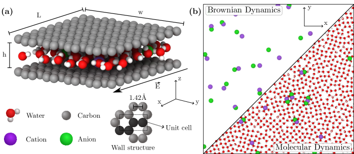
Figure 1: System studied in this paper. (a) Simulation setup for the molecular dynamics simulation. The wall are generated from a unit cell of 4 carbon atoms, in black in the structure. (b) Comparison of Brownian dynamics (top left) and molecular dynamics (bottom right) simulations at a same ionic density.

Two different simulation methods are used throughout this paper. In all-atom molecular dynamics (MD), the entire system (water molecules, ions and atoms from the channel walls, see Figure 1(a)) is simulated using classical Lennard-Jones and Coulombic forcefields and solving Newton’s equations of motion. In Brownian dynamics (BD), on the other hand, water and channel walls are treated implicitly, and only the positions of ions are tracked using overdamped Langevin equations. They are carried out using GROMACSAbraham et al. (2024) and LAMMPSThompson et al. (2022) softwares, respectively. Both equilibrium (EMD and EBD, without any external electric field) and non equilibrium simulations (NEMD and NEBD, with an external electric field) are used. The trajectory are obtained from simulation results using the MDAnalysisGowers et al. (2016) Python library, and visualized with OvitoStukowski (2010). Structure analysis of ion clusters is done using the network analysis Python library NetworkX Hagberg, Swart, and Schult (2008).

I.1 All-atom molecular dynamics

Molecular dynamics simulations consist of two sheets of fixed carbon atoms, with periodic boundary condition. In order to reproduce the crystalline structure of graphene, a rectangular unit cell of size $\sqrt{3}d_{c}\times 3d_{c}$ is created, corresponding to 4 carbon atoms, where $d_{c}=1.42\ \text{\AA}$ is the carbon-carbon distance (see Figure 1 for the definition of the unit cell). This cell is replicated 81 times along the $x$ direction and 46 times along the $y$ directions for each sheet. Both sheets are separated by a distance $h$, which creates a slit of height $h=7\ \text{\AA}$. Because of periodicity, we extend the simulation box to 20nm in the z direction to avoid interaction between periodically replicated images. This gives a total simulation box of size $19.9\ \text{nm}\times 19.6\ \text{nm}\times 20\ \text{nm}$. The inside of the slit is filled with water ad ions consisting in 2 identical mono-atomic species with a varying charge $\pm Ze$. The number of water molecules and ions are respectively $N_{w}=4500$ and $N_{+}=N_{-}=N=100$. This corresponds to a ionic concentration inside the slit of 0.6 M. The procedure used to estimate the number of water molecules in this geometry is presented in supplementary material (Section S2).

Water molecules are modeled using the SPC/E modelBerendsen, Grigera, and Straatsma (1987) (3 point charges model) and maintained rigid with the SHAKE algorithmRyckaert, Ciccotti, and Berendsen (1977). Short-range interactions are modeled using Lennard-Jones (LJ) potentials. The cut-off distance for LJ and Coulombic interactions is 1.2 nm. The atom mass, charges and Lennard Jones parameters are summarized in the supplementary material (Table S1). For both ions we use the same LJ parameters and masses (which are taken from the sodium force-field) with opposite charges. Long-range Coulombic interactions are treated with the smooth particle-mesh Ewald methodDarden, York, and Pedersen (1993); Essmann et al. (1995). When initializing the simulation, the total energy is minimized using the steepest descent minimization algorithm.

Simulations are performed in the NVT ensemble using the velocity VerletSwope et al. (1982) algorithm with a timestep $\text{d}t=1$ fs. The system is coupled to a thermostat at 300K using velocity rescaling with a stochastic termBussi, Donadio, and Parrinello (2007). The simulation runs for $1.5\times 10^{7}\ \text{d}t=$15 ns, and the first 5 ns are discarded for thermalization during analysis.

I.2 Brownian dynamics

I.2.1 Equation of motion

In BD, ions evolve in a 2D continuous space representing the nanochannel. The following equation of motion is solved for each ion $i$:

$$\frac{\text{d}\vec{r}_{i}}{\text{d}t}=\frac{D}{k_{B}T}\left(z_{i}eE\vec{u}_{x}-\vec{\nabla}U_{i}\right)+\sqrt{2D}\vec{\eta}_{i}(t),$$ (1)

where $z_{i}=Z$ for cation and $z_{i}=-Z$ for anions, $E$ is the external field, $D$ is the diffusion coefficient (identical values for both cations and anions), $U_{i}$ is the total potential felt by the ion i, and the $\vec{\eta}_{i}$ are independent 2D white noise forces:

$$\langle\vec{\eta}_{i}(t)\rangle=\vec{0},\quad\langle\vec{\eta}_{i}(t)\cdot\vec{\eta}_{j}(t^{\prime})\rangle=\delta_{ij}\delta(t-t^{\prime})$$ (2)

The cut-off distance for the interaction between the ions is $r_{c}=20$ nm. The shape of the inter-ions potential is the object of the next subsection.

The strength of the interaction can be tuned either by changing the charge of the ions, or the temperature. Without explicit solvent, both techniques should yield identical results. In the following, we choose to vary the temperature. The diffusion coefficient is adjusted in order to keep the relaxation time constant, with value:

$$\tau=\frac{Dm}{k_{B}T}=9.6\ \text{fs}$$ (3)

We choose $m=23\ \text{uma}$ for both ions. This assures that the ionic mobility remains the same across simulations at different temperatures.

The system consists of $N_{+}=N_{-}=N$ ions in a 2D slit of dimension $L\times w$. In section II, we use $N=100$ ions, in a box of lendth and width $L=w=100$ nm, for a total simulations times of $10^{6}$ timesteps. In section III, we use $N=4000$ ions, in a box of length $L=2000$  nm and width $w=200$  nm, for a total simulations times of $10^{5}$ timesteps. For all BD simulations, the width $w$ of the slit is chosen to have a constant ionic density of $10^{16}\ \text{atom}.\text{m}^{-2}$ for each ions, corresponding to a concentration of 0.025 M. The timestep is set to 5 ps.

I.2.2 Interaction potential

In BD, water and channel walls are treated implicitly. In bulk simulations with no walls, this amounts to introducing the relative dielectric constant $\varepsilon_{w}$ of water; here, we also must take into account the dielectric properties of the walls, which in general strongly contrast with waterSchlaich, Knapp, and Netz (2016); Fumagalli et al. (2018). Dielectric mismatch between water and walls results can be accounted for through image charges within the wall in the presence of ions. Reference Kavokine, Robin, and Bocquet (2022) shows that in a slit of height $h$, with wall of permittivity $\varepsilon_{s}$ and water of permittivity $\varepsilon_{w}$, this effect renormalises ion-ion interaction, so that the pairwise potential becomes:

$$\beta V_{ij}(r_{ij})=-\frac{\text{sign}(z_{i}z_{j})}{T^{*}}\log\left(\frac{r_{ij}+C}{r_{ij}+\xi}\right),$$ (4)

where $z_{i}=\pm 1$ is the charge of the ion $i$, $\xi$ is the dielectric length, $T^{*}$ is the reduced Coulomb temperature, a dimensionless measure of temperature, $C\,(\sim\text{\AA})$ is a short distance cut-off, $r_{ij}$ is the distance between the ions and $\beta=1/k_{B}T$.

The dielectric length $\xi$ depends only on the geometry of the slit, and not on the properties of the ions. We have:

$$\xi=\frac{\varepsilon_{w}}{2\varepsilon_{s}}h=13.8\text{nm},$$ (5)

for ions in water ($\varepsilon_{w}\sim 80$) in a slit of height $h=7\text{\AA}$, confined by walls with a very low dielectric constant ($\varepsilon_{s}=2$). This length corresponds to the typical length below which the electric field created by the ions is confined because of dielectric contrast. While in MD simulations electrostatic interactions follow the Coulomb’s law, it is useful to notice that they correspond to $\varepsilon=1$ (or $\xi=27.6$ nm), since we model channel walls by a single carbon atomic layer followed by a slab of empty space. An other interesting limit is the case of a total confinement of the electric field $\xi\to\infty$, for which we recover the logarithmic potential of a 2D Coulomb gas.

The short range cutoff $C=3\text{\AA}$ is an additional parameter that is chosen to avoid divergences of the potential at short ionic distances, without requiring an additional repulsive potential.

The reduced Coulomb temperature $T^{*}$ is an non dimensional parameter which measures the inverse of the interaction strength:

$$T^{*}=\frac{2\pi\varepsilon_{0}\varepsilon_{w}h}{Z^{2}e^{2}\mathcal{K}}k_{B}T,$$ (6)

where $\mathcal{K}=1.11$ is a geometric factor Robin, Kavokine, and Bocquet (2021). The interaction can be controlled by changing either the charges of the ions, or the temperature. In relevant experimental conditions, $T$ is usually fixed to 300K, and $Z$ is varied by using salts of various valence, $T^{*}=0.1$ corresponds to divalent ions and $T^{*}=0.4$ to monovalent ions. For practical reason, we rather fix in this work $Z=2$ and vary the temperature $T$ as a way of tuning interactions continuously over a wide range of strengths.

Finally, the total effective interaction potential felt by an ion in Brownian dynamics simulation is given by:

$$U_{i}=\sum_{j\neq i}V_{ij}^{c}(r_{ij}),$$ (7)

where:

$$V_{ij}^{c}(r_{ij})=\left\{\begin{array}[]{cc}V_{ij}(r_{ij})&\quad\text{if }r_{ij}<r_{c}\\ 0&\quad\text{otherwise}\end{array}\right.$$ (8)

I.3 Convention for correlations functions

The total pair correlation function is defined as:

$$g_{p}(\vec{r})=\frac{\mathcal{A}}{4N^{2}}\left\langle\sum_{i}^{2N}\sum_{j\neq i}^{2N}\delta(\vec{r}-(\vec{r}_{i}-\vec{r}_{j}))\right\rangle,$$ (9)

where $\mathcal{A}=Lw$ is the area of the slit, $\vec{r}_{i}$ is the position of ion $i$, and where $\langle\cdot\rangle$ denotes an ensemble average. Without external field, the system is symmetric by rotation, and the radial pair correlation functions can be used instead:

$$g_{p}(r)=\frac{1}{2\pi r}\frac{\mathcal{A}}{4N^{2}}\left\langle\sum_{i}^{2N}\sum_{j\neq i}^{2N}\delta(r-|\vec{r}_{i}-\vec{r}_{j}|)\right\rangle.$$ (10)

We can alternatively define $g_{\text{op}}$ and $g_{\text{id}}$ the pair correlation functions for respectively oppositely charged and identically charged ions :

$$\begin{array}[]{ccc}g_{\text{op}}(r)&=&\frac{1}{2\pi r}\frac{\mathcal{A}}{N^{2}}\left\langle\sum_{i,\text{cations}}^{N}\sum_{j,\text{anions}}^{N}\delta(r-|\vec{r}_{i}-\vec{r}_{j}|)\right\rangle\\ g_{\text{id}}(r)&=&\frac{1}{2\pi r}\frac{\mathcal{A}}{N^{2}}\left\langle\sum_{i,\text{cations}}^{N}\sum_{j\neq i,\text{cations}}^{N}\delta(r-|\vec{r}_{i}-\vec{r}_{j}|)\right\rangle\end{array}$$ (11)

$g_{\text{op}}$ is invariant under inversions of anions and cations, however $g_{\text{id}}$ is slightly asymmetric - even for symmetric anion and cation - because of the structure of water molecules. In the following we take the average of both anion-anion and cation-cation pair correlation functions.

In practice, we compute all the $2N^{2}N_{t}$ unique ionic distances, where $N_{t}$ is the number of simulation steps used, and $N$ is the number of ions. The distance between ions are corrected to take into account the periodicity. Radial pair histograms are computed every 5 ns ($10^{3}$ timesteps), for a total simulations length of 5 $\mu$s ($10^{6}$ timesteps), and the first 500 ns are discarded. In order to estimate the uncertainty on those quantity, we split the time interval into 10 windows, and we compute the standard deviation of the window averages.

The running coordination number $N_{\text{op}}(r)$ and $N_{\text{id}}(r)$ can be obtained upon integration of the radial pair correlation function of respectively opposite and identical ions. It corresponds to the number of ions in a shell of radius $r$ around any ions:

$$N_{\text{op}}(r)=2\pi\frac{N}{\mathcal{A}}\int_{0}^{r}g_{\text{op}}(u)u\text{d}u.$$ (12)

$$N_{\text{id}}(r)=2\pi\frac{N}{\mathcal{A}}\int_{0}^{r}g_{\text{id}}(u)u\text{d}u.$$ (13)

The counter charge density around an ion can be defined as:

$$q(r)=-\frac{1}{4\pi rN}\left\langle\sum_{i}^{2N}\sum_{j\neq i}^{2N}\text{sign}(z_{i}z_{j})\delta(r-|\vec{r}_{i}-\vec{r}_{j}|)\right\rangle,$$ (14)

$q$ can be integrated to obtain:

$$Q(r)=2\pi\int_{0}^{r}q(u)u\text{d}u=N_{\text{op}}(r)-N_{\text{id}}(r),$$ (15)

which corresponds to the total counter charge in a disk of radius $r$ around an ion. Those functions are normalized by the central ion charge, such that $Q(0)=0$, and $Q(r\to\infty)=1$, which corresponds to global neutrality of the system.

Adding an external electric field breaks the isotropy of the system. In this case, the running coordination number $N(r,E)$ can still be defined, but it does not exactly have the same physical meaning, as the anisotropic correlation are integrated on a circle.

I.4 Ionic current

In simulations where an external field $E$ is applied, by using translation invariance along the direction of the field, we compute the ionic current using:

$$j=Ze\frac{N}{h\mathcal{A}}\left(\langle v_{+}\rangle-\langle v_{-}\rangle\right),$$ (16)

where $v_{+}$ and $v_{-}$ are respectively the velocity of the cations and the anions along the direction of the field. The velocities are computed every $10^{3}$ time-steps. We estimate the uncertainty of results by splitting the whole trajectories into 10 windows, and by computing the standard deviation of the window averages.

Upon integration across the slit, the ionic current intensity is given by:

$$I=hwj.$$ (17)

For non interacting ions, the current is given by:

$$j_{0}=\frac{2N}{h\mathcal{A}}\frac{(Ze)^{2}D}{k_{B}T}E,$$ (18)

which is the regular Ohm’s law. We finally compute the conductivity using:

$$\sigma(E)=\frac{j(E)}{E},$$ (19)

and we define the Ohmic conductivity:

$$\sigma_{0}=\frac{2N}{h\mathcal{A}}\frac{(Ze)^{2}D}{k_{B}T}$$ (20)

In Brownian dynamics simulations, as we have chosen the ionic mobility and the ionic charges to be constant across all the simulations, the Ohmic current and conductivity are the same for all $T^{*}$.

I.5 Ionic clusters

When the correlations between the ions becomes strong enough, some ions can be considered as bonded. Then, the distribution of the ions inside the system can be seen as node in a graph, in which bonded ions corresponds to connected nodes. We can define ionic cluster as the connected components of this graph, using standards tools from graph theory Hagberg, Swart, and Schult (2008). This is particularly relevant in MD simulations.

We define $N_{l}$ as the number of clusters of size $l$, and $n_{l}$ the density of ions in clusters of size $l$:

$$n_{l}=\frac{lN_{l}}{2N}.$$ (21)

The conservation of the total number of ions yields:

$$\sum_{l}n_{l}=\frac{1}{2N}\sum_{l}lN_{l}=1.$$ (22)

If the number of cations and anions is different inside a given cluster, the cluster will have a net charge $z_{c}e$. It is in particular always the case for clusters with an odd number of ions. We will define the free carrier density as:

$$n_{f}^{\text{cluster}}=\frac{1}{2N}\sum_{c}\frac{z_{c}^{2}}{Z^{2}}.$$ (23)

In practice, we only observe clusters with charges 0 or $\pm Z$. We hypothesise that clusters with multiple charge defects are too short-lived to be relevant. In this case the above formula can be simplified:

$$n_{f}^{\text{cluster}}\sim\frac{N_{c}}{2N}=\frac{\sum_{l\text{ odd}}N_{l}}{2N},$$ (24)

where $N_{c}$ is the total number of cluster.

II Ion pairing and screening

In this section, we study the formation of ionic pairs using both Brownian dynamics simulations and theoretical analysis. In particular, we determine the average number of pairs both at thermal equilibrium, but also in non-equilibrium conditions under an external field. We show that the system undergoes a conductor/insulator phase transition reminiscent of the 2D Kosterlitz-Thouless transition. We analytically predict the system’s critical temperature, which is found to slightly deviate from the usual KT result due to the quasi-2D nature of confined electrolytes.

II.1 Bjerrum pairing

In both MD and BD simulations, we observed that oppositely charged ions often forms tightly bound pairs (see Figure 1.(b)). These pairs are absent in bulk aqueous systems, and are therefore a direct consequence of nanoscale confinement.

The strength of the ionic interactions can be quantified by the Bjerrum lengthBjerrum (1926) $l_{B}$, defined as:

$$\beta V(l_{B})=k_{B}T.$$ (25)

It is the typical length which compares ion interaction with thermal energy. For a 3D system, the Bjerrum length is defined as

$$l^{\text{bulk}}_{B}=\frac{e^{2}}{4\pi\epsilon_{0}\epsilon_{w}k_{B}T},$$ (26)

while for 2D systems, a rough estimate is

$$l^{\text{2D}}_{B}\sim\frac{\xi}{T^{*}}.$$ (27)

This can be used to compare the interaction in each systems:

$$\frac{l^{\text{2D}}_{B}}{l^{\text{bulk}}_{B}}\simeq\frac{\varepsilon_{w}}{\varepsilon_{s}}\gg 1.$$ (28)

In bulk water, $l_{B}^{\text{bulk}}=0.7$nm, meaning that long-range interactions between ions are essentially negligible compared to thermal noise. In the slit this is not the case anymore, as the Bjerrum length is orders of magnitude larger. The possibility for the ions to form pairs, called Bjerrum pairs, has to be taken into account in our analysis.

In order to quantify ionic pairing, we can introduce the free ion fraction $n_{f}(E)$ and the ion pair fraction:

$$n_{p}(E)=1-n_{f}(E).$$ (29)

$n_{f}=0$ and $n_{f}=1$ correspond respectively to fully paired and fully dissociated electrolytes. This fraction can be separated into 2 contributions: a proportion $n_{f}(0)$ of ions which remain free, even in the absence of external field, and a quantity $\delta n_{f}(E)$ coming from additional pairs breaking under the effect of the electric field, in a process known as the second Wien effectKaiser (2014); Onsager (1934):

$$\delta n_{f}(E)=n_{f}(E)-n_{f}(0).$$ (30)

In what follows, we study the properties of both $n_{f}(0)$ and $\delta n_{f}(E)$. The former is related to the system’s conductivity at vanishingly low electric field, while the latter describes non-linear conduction outside of equilibrium.

II.2 Determination of the free ion fraction at equilibrium

II.2.1 Definition of the charge carrier density

Pairs being neutral, they do not contribute to conduction under an external field. By applying a constant electric field in Brownian simulations, we can obtain the fraction of charge carriers by comparing the measured ionic current to the Ohmic current:

$$n_{f}(E)=\frac{j(E)}{j_{0}(E)}.$$ (31)

This definition of an ionic pair has the advantage of being the closest to what could be measured in experiments, in addition to being very convenient to compute. In fact, it effectively counts the fraction of charge carriers only if we can neglect higher-order correlations between ions (which tend to impede conduction compared to the Ohmic case), or equivalently if we assume the mobility of individual ions not to vary with the field. We make this assumption in the following, since we expect the non linearity of the system to be dominated by the variation of the fraction of charge carriers (second Wien effect), and not by the variation of the mobility (first Wien effectKaiser (2014); Kaiser et al. (2013), and Debye-Hückel correlations in generalBerthoumieux, Démery, and Maggs (2024)).

However, Equation (31) is not suited for the measure of the ionic current under a very weak electric field, when the signal-to-noise ratio becomes too low. We attribute this noise to thermal fluctuations, as well as finite-size effects, which become particularly prominent when the proportion of free ions is small (i.e. at low temperature and low applied field). In general, this formula gives an accurate result when $E\gtrsim 2\times 10^{7}$ V/m, which is unfortunately too large for a direct estimate of $n_{f}(0)$.

In the next paragraph, we develop an alternative method to estimate the value of the free ion fraction in the absence of external field. We will make use of an alternate definition of ion pairs, based on correlation functions. We show that this definition is robust regardless of the magnitude of the external field. We will therefore use it as a proxy to estimate the free ion fraction at equilibrium.

II.2.2 Determination from correlation functions

We define a typical length scale $d(E)$ associated with the formation of pairs through the correlation function. We assume a separation of the ions into 2 different types of cluster, the free ions and pairs. By splitting the sum in the definition of $g_{\text{op}}(r)$ between paired and unpaired ions, we can rewrite:

$$N_{\text{op}}(r,E)=n_{p}\int_{0}^{r}\rho_{\text{intra}}(r)\text{d}r+(N-n_{p})\int_{0}^{r}\rho_{\text{inter}}(r)\text{d}r,$$ (32)

where $\rho_{\text{intra}}$ and $\rho_{\text{inter}}$ are respectively the correlation functions of ions within a same cluster (short distances) and correlations of ions in different clusters (large distances). Both of them vary with the external field. When the overlap between those distributions is small, we can define an intermediate length $d(E)$ between intra and inter cluster correlation, which corresponds to the maximal size of a pair. When $r\simeq d(E)$, the first integral is close to 1, when the second one remains close to 0. This yields:

$$N_{\text{op}}(d(E),E)=n_{p}(E).$$ (33)

In other words, $N_{\text{op}}$ exhibits a plateau (see Figure S2), associated to a minimum of $g_{\text{op}}$. For $T^{*}\gtrsim 0.1$, we do not observe any minima in the correlation functions, which indicates that a geometric criterion is not adapted for our system. Yet, as the fraction of charge carrier is still well defined in presence of external field, we can use this number to define a typical distance between paired ions $d(E)$:

$$N_{\text{op}}(d(E>0),E>0)=1-n_{f}(E>0),$$ (34)

where $n_{f}(E>0)$ is computed from transport simulations using equation (31). We then extrapolate the value of the pair distance without external field $d(E=0)$, by assuming that the pair distance decays exponentially with the field. We can finally estimate the free ion fraction without external field as the value of the running coordination function at $d(0)$. The whole procedure is shown for $T^{*}=0.4$ in Figure S1.

II.3 Pairing transition

II.3.1 Comparison with the 2D Coulomb gas

We now use the method described above to compute the free ion fraction without an external field as a function of temperature $T^{*}$. Below $T^{*}\lesssim 0.15$, there is a large uncertainty as the measured currents are small. However, in this regime, the approach using the coordination function demonstrate the absence of any free ion, see Figure S2): the system is fully paired.

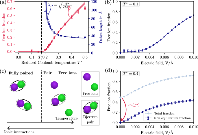
Figure 2: Pairing transition and evolution of the free ion fraction with the electric field (a) (Red points) Free ion fraction from BD simulation for various reduced Coulomb temperature. (Red lines) Fit of the free ion fraction for an infinite order phase transition. (Blue points and line) Debye length obtained from the the free ion fraction using Equation (35). (b) (Circle) Free ion fraction as a function of the electric field, obtained from the measure of the ionic current, at $T^{*}=0.1$. The main source of uncertainty is the uncertainty on the current. (Diamond) Value at equilibrium. (c) Schematic of the phase transition. At small reduced Coulomb temperature or equivalently high ionic interaction, the system is fully paired. Otherwise, there is some remaining free ions. (d) (Light blue circle) Free ion fraction as a function of the electric field, obtained from the measure of the ionic current, at $T^{*}=0.4$. The uncertainty is small as we measure a larger current. (Light blue diamond) Value at equilibrium, see (a). (Blue circle) Contribution from the non equilibrium free ion only, obtained by subtracting the value at equilibrium to the total current. Its uncertainty is dominated by the uncertainty of the equilibrium value.

In order to better understand the behaviour of our system, it is interesting to compare to the case of a purely 2D Coulomb gas $\xi\to\infty$. In this ideal system, there is a phase transition between a fully paired system and a mixture of free ions and pairs. This transition is identical to the Kosterlitz-Thouless transition Kosterlitz and Thouless (1973); Levin (2002) for the 2D XY model, with a same critical temperature $T^{*}=0.25$. A full analytical treatment of this transition has been detailed elsewhere Levin (2002); in the following, we only sketch the main arguments behind this comparison.

The free energy cost of breaking a pair at thermal equilibrium is roughly the electrostatic free energy of creating the Debye correlation cloud around each ion forming the pair. Indeed, every free ion is surrounded by an atmosphere of opposite charge, extending over a typical scale known as the Debye length:

$$\lambda_{\text{D}}=\sqrt{\frac{T^{*}}{4\pi n_{f}\rho}}.$$ (35)

In the limit where the ionic concentration is not too highRotenberg, Bernard, and Hansen (2018), it should corresponds to the correlation length of electrostatic interactions in the system i.e. the decay length of the correlation function between free ions only.

Overall, the free energy of breaking a pair scales like:

$$\beta\Delta F\sim-\frac{1}{T^{*}}\log\lambda_{\text{D}}/r_{0},$$ (36)

where $r_{0}$ is the ionic size (here set by the short distance cut-off $C$ of the interaction potential). The chemical equilibrium between pairs and free ions then read:

$$n_{p}=1-n_{f}=Kn_{f}^{2}e^{-\beta\Delta F}\propto n_{f}^{2-1/2T^{*}},$$ (37)

with $K$ a constant that depends on the exact criterion used to define pairs (e.g., on the threshold in distance under which two ions are assumed to form a pair). For $T^{*}<1/4$, this equation cannot be solved for $n_{f}$ since $2-1/2T^{*}<0$. This indicates that chemical equilibrium between pairs and free ions no longer holds, and the system undergoes a phase transition where all ions pair up.

Figure 2 shows the evolution of the free ion fraction with the temperature obtained in our simulations (red symbols). We observe that the free ion fraction decreases when we increase the interaction between the ions, and vanishes for $T_{c}^{*}\simeq 0.17$, a value rather close to the theoretical prediction $T^{*}_{c}=1/4$. We will show in next section that this slight difference can be attributed to deviations to the perfect Coulomb gas (limit $\xi\to\infty$) in our BD simulations ($\xi=13.8$ nm)

Let us now characterize the nature of this phase transition. A hallmark of the Kosterlitz-Thouless transition is that it is of infinite order – in other words, it does not entail a symmetry breaking, and the system’s correlation length depends in a non-algebraic way on the temperature above the transition. Again, this can be shown through simple arguments as follows. For $T^{*}$ sligthly above $T^{*}_{c}$, the system is still almost fully paired, so that $n_{p}\simeq 1$. From the chemical equilibrium (Equation (37)), we obtain that:

$$n_{f}\sim K_{2}^{-1/(2-1/2T^{*})}\sim e^{-\frac{T^{*}/2}{T^{*}-T^{*}_{c}}},$$ (38)

Where $K_{2}$ is a temperature-independent constant (which depends on $K$). Since $\lambda_{\text{D}}\sim n_{f}^{-1/2}$, we have, for $T^{*}\gtrsim T^{*}_{c}$:

$$\lambda_{\text{D}}\sim e^{\frac{T^{*}/4}{T^{*}-T^{*}_{c}}},$$ (39)

which shows that indeed the correlation length is non-algebraic (in particular, no critical exponent can be defined).

We represent the value of $\lambda_{\text{D}}$ as computed in the simulation in Figure 2 (blue symbols). We fit its temperature dependence above the transition with the ansatz:

$$\lambda_{D}(T^{*}\to T_{c}^{*+})\sim Ae^{\frac{T^{*}/4}{T^{*}-T_{c}^{*}}},$$ (40)

where $A$ and $T_{c}^{*}$ are chosen to reproduce our data. The red and blue curves in Figure 2 shows the result of this model. We obtain a very good agreement for a critical temperature $T_{c}^{*}\sim 0.17$. In particular, we recover the non-algebraic nature of the correlation length.

Despite this difference in the exact value of the critical temperature, we can conclude that the phase transition observed in the simulations is indeed in the same universality class as the one of the exact 2D Coulomb gas, or of the Kosterlitz-Thouless transition. In particular, we find that it is a transition of infinite order, as shown by the non-algebraic decay of the correlation length.

II.3.2 Theoretical analysis with finite dielectric length

In the case where confinement is imperfect, $\xi<\infty$ and the above transition is found to occur at a lower temperature than predicted by the perfect Coulomb gas ($\xi\to\infty$). In this section, we provide a theoretical analysis of this phenomenon and compute the approximate value of the transition temperature. Assuming that ions have a radius $r_{0}$ and cannot interpenetrate, we find that at the Debye-Hückel level, the ionic atmosphere surrounding each ions creates an electrostatic potential $\psi$ on ions:

$$\psi=\frac{1}{T^{*}}\left[\frac{\xi}{\kappa_{\text{D}}r_{0}(r_{0}+\xi)}\frac{K_{0}(\kappa_{\text{D}}r_{0})-K_{0}(\kappa_{\text{D}}(r_{0}+\xi))}{K_{1}(\kappa_{\text{D}}r_{0})-K_{1}(\kappa_{\text{D}}(r_{0}+\xi))}\right],$$ (41)

with $\kappa_{\text{D}}$ the inverse Debye length. Note that in the case of the perfect 2D Coulomb gas, the same quantity reads:

$$\psi=\frac{1}{T^{*}}\left[\frac{K_{0}(\kappa_{\text{D}}r_{0})}{\kappa_{\text{D}}r_{0}K_{1}(\kappa_{\text{D}}r_{0})}\right].$$ (42)

By using a Debye charging process, one can show that the excess chemical potential of free ions is directly linked to $\psi$:

$$\mu_{e}=\frac{1}{2}\psi.$$ (43)

The number of free ions is then given by, assuming pairs behave like ideal solutes:

$$n_{p}=1-n_{f}=Kn_{f}^{2}e^{2\mu_{e}}.$$ (44)

In the case $\xi<\infty$, the solution of Equation (44) cannot be obtained analytically, but can be solved numerically. In Figure 3.(a) we plot the evolution of the free ion fraction with the density above ($T^{*}=0.15$) and below ($T^{*}=0.35$) the critical temperature.

At low temperature, we observe a discontinuity in the free ion fraction at a density $\rho_{t}(T^{*})$ (see red curve in 3). This defines a transition line between a system with a low fraction of free ion below the line, and a large fraction of free ion above. This behaviour is very similar to what is obtained in the perfect 2D case. The main difference is that instead of a fully paired phase $n_{f}=0$, few ions can remain dissociated.

In the perfect 2D case, it has been shownLevin (2002) that the transition line stops with a tricritical point $(T_{c}^{*},\rho_{t}(T_{c}^{*}))$ at the critical temperature $T_{c}^{*}=0.25$. Indeed, when $\rho<\rho_{t}(T_{c}^{*})$ and $T^{*}<T_{c}^{*}$, Equation (44) has no solution: The system is fully paired. This defines a critical line at $T^{*}=T_{c}^{*}$ that stops a the tricritical point. By analogy, at finite dielectric length, we observe that the discontinuity stops when $T^{*}\gtrsim T_{c}^{*}=0.183$, providing an estimate of the critical temperature. This value is in particular very close to the value obtained from BD simulations, $T_{c}^{*}=0.17$.

In order to compare our theoretical results with our BD simulations, we plot in Figure 3.(b) the evolution of the free ion fraction with the reduced Coulomb temperature for $\xi=13.8$ nm and for the perfect 2D case. To be consistent we use the same ionic density than BD simulations ($10^{16}$  atom.m^-2). This density is below the tricritical point (for both system), and we indeed observe a transition at the critical temperature, between a phase with a low free ion fraction (fully paired for the perfect 2D case), and a phase with a large free ion fraction.

We finally note that for system with small $\xi$ such that liquid/wall with low dielectric contrast, or when the wall have a large Thomas-Fermi length Kavokine, Robin, and Bocquet (2022) (i.e. insulator or bad metal), the screening of the wall becomes dominant and the transition is not visible.

In Figure 3.(b), we plot the free ion fraction obtained in last subsections. Simulations and theories agrees very well qualitatively, in particular close to the transition. The discrepancies can be explained by the very different treatment of short range interactions in both system, yielding to different values of $K$ (defined in Equation (36)) and ionic radius $r_{0}$.

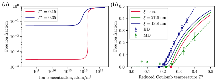
Figure 3: Theoretical predictions of the phase transition. (a) Evolution of free ion fraction with density below the transitions ($T^{*}=0.15$, in red) and above the transition ($T^{*}=0.35$, in blue), obtained from numerical solution of Equation (44). We use $\xi=13.8$ nm to match BD simulations. (b) Theoretical free ion fraction for the exact 2D Coulomb gas (red) and at finite dielectric length 13.8 nm (blue, comparable to BD simulations) and 27.6 nm (green, comparable to MD simulations), computed using Equation (44). The position of the transition temperature is shown by a cross. The result from respectively BD and MD simulations are plotted in blue and green, as well as the fit defined in Equation (40). In those cases the critical temperature obtained by the fit is indicated by a cross on the x axis.

II.4 Effect of the short-range interactions

II.4.1 Formation of ionic clusters

In previous sections, the absence of short distance repulsion between ions weakened the ionic structure, making the distinction between free ions and pairs quite blurry. Without repulsive potential, the distance between ions in a pair fluctuates around 0. As there is no permanent dipoles in this case, their interactions with other ions are very weak. In all atom MD, where ions also interact through repulsive LJ interactions, pairs fluctuates around a finite distance (see Figure 1.(b) and Figure 4.(a)). In this case, interaction with pairs are no longer negligible, allowing the formation of more complex structure.

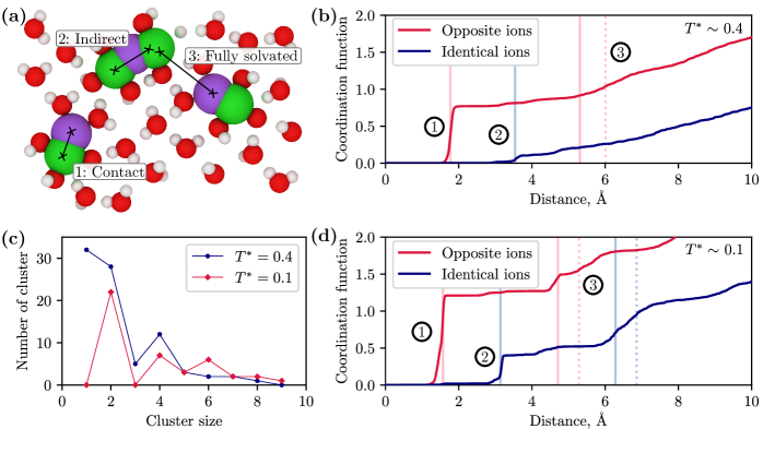
Figure 4: Structure in explicit solvent simulations and its relation with correlation functions (a) Screenshot from EMD simulations for $T^{*}=0.1$. We observe 2 types of direct bonding, the contact bonds (1) when there is no water between ions, and solvent separated bonds (3) when both ions are bond, with solvent in between. We also observe indirect bonding (2) between ions, which is a consequence of the presence of clusters. (b) and (d) Running coordination function as a function of the distance between the ions, respectively for a reduced Coulomb temperature of 0.4 (monovalent ions) and 0.1 (divalent ions). The red and blue curves corresponds respectively to correlation between opposite and identical ions. We also identifies some of the well defined jump, which corresponds to spike in the correlation function. The plain pink vertical line corresponds to the contact bonds. The plain pink and light blue line corresponds to multiples of the distance between contact bond, and corresponds to indirect bond in linear chains of ions with alternating sign. The dotted pink and blue vertical line corresponds to solvent separated bonds. (c) Cluster size distribution $N_{l}$ defined as the number of clusters of connected ions (ions at distances smaller than $7\text{\AA}$ from at least one other ion in the cluster). In blue and red respectively the data for a reduced Coulomb temperature of $0.4$ (monovalent ions) and $0.1$ (divalent ions).

Figure 4 shows respectively the oppositely and identically charged ions running coordination numbers $N_{\text{op}}$ and $N_{\text{id}}$, for monovalent ions ($T^{*}\sim 0.4$, panel (b)) and divalent ions ($T^{*}\sim 0.1$, panel (d)). Both display well defined jumps, corresponding to thin peaks in the correlation function i.e. stiff minima in the free energy. This is a direct consequence of the presence of repulsive interaction.

From comparative analysis between the simulations movies 4.(a) and coordination curves 4.(b) and (d), we can relate the structures and the peaks. We observe both direct bonds between opposite ions (non mediated by other ions) and indirect bonds (mediated by other ions, could not exist in an ionic pair). Most of the direct bonds are contact bonds at small distances $d\sim 2\ \text{\AA}$. We also observe some solvent separated bonds, mediated by water molecules, at larger distances $d\sim 6\ \text{\AA}$.

The position of the peaks associated to indirect bonds gives us information on the structure of the clusters. For example in our system, we mostly observe peaks at multiples of the size of contact bond, which is a signature of the predominance of linear ionic chains, in agreement with was can be seen in simulations movies.

Other worksRobin, Kavokine, and Bocquet (2021); Zhao et al. (2021) that used different simulations techniques reported various possible structures of ionic clusters, depending for example on the chemical nature of ionsRobin, Kavokine, and Bocquet (2021); Zhao et al. (2021) or of the wallFong et al. (2024). Overall, the relations between short-range interaction and short-range structure seem non universal and is in practice difficult to analyse. Instead, we now focus on long-range correlations, in comparison with BD simulations.

II.4.2 Pairing transition in all-atom simulation

As in Brownian dynamics we could use transport simulation in order to study pairing. Indeed, from the definition of the free carrier density (Equation (23)):

$$n_{f}^{\text{cluster}}(E)=\frac{j(E)}{j_{0}(E)},$$ (45)

if we neglect any variation of the mobility of the field. However, as in BD simulations, this definition is not adapted to very small field. Instead, we can use the following geometric criterion.

We can define a cluster as an ensemble of ions that are at distance smaller than a distances $d_{c}$ to at least another ion in the cluster. $d_{c}$ is a small distance, below which we consider 2 opposite ions to be bound. We will use in the following $d_{c}=7\text{\AA}$ for every charge. This allows to take into account both the contact bonds (vertical pink lines in 4) and the solvent separated bonds (vertical dashed pink lines in 4).

The distribution $N_{l}$ of clusters of size $l$ is shown in Figure 4.(c) for a reduced Coulomb temperature of 0.4 (in blue), corresponding to monovalent ions, and 0.1 (in red), corresponding to divalent ions. We observe a global exponential decay of the cluster numbers with their size, and clusters with even number of ions are more abundant.

This can be explained by the fact that clusters with an odd number of ions are charged, as they cannot have the same number of anions and cations. However, we only observe neutral even clusters. The disparity is a consequence of the free energy cost to have a charged cluster. As expected, the disparity between odd and even clusters increase when the ionic charges is increased.

In order to quantify this effect, the free charge carrier density is extracted from MD simulations. The result is shown in Figure 3.(b). Below $T^{*}\simeq 0.25$, the free charge carrier obtained from MD simulations is close to zero, and increase above, following the same tendency of BD simulations. We can use Equation (40) to fit the simulations points, and estimate the critical temperature. The critical temperature estimated this way (green cross in Figure 3) is coherent with the theoretical prediction (green line in Figure 3). As in BD simulations, the general curve does not exactly match the theoretical curve, as a consequence of the different treatment of the short-range interaction. In addition of that, the cluster density is MD simulations might evolve with the reduced Coulomb temperature.

At small reduced Coulomb temperature, the small deviation from 0 at small temperature can be explained by the fact that the charge density stabilises on very long timescales, because of the slow dynamic of the clusters.

We can write more formally the analogy between MD and BD system from the definition of $q(r)$. We can separate the sum between ions in same (intra) or different (inter) clusters. We obtain:

$$q(r)=(1-n_{f}^{\text{cluster}})q_{\text{intra}}(r)+n_{f}^{\text{cluster}}q_{\text{inter}}(r).$$ (46)

Where $q_{\text{intra}}$ and $q_{\text{inter}}$ are normalised to 1. For each ion $i$ inside a cluster $c$, we can write $\vec{r}_{i}=\vec{r}_{c}+\delta\vec{r}_{i}$, where we expect $\delta\vec{r}_{i}$ to be negligible compared to the distance between clusters. Neglecting multi-polar terms yields to:

$$q_{\text{inter}}(r)\sim-\left\langle\sum_{c}\sum_{c^{\prime}\neq c}\frac{z_{c}z_{c^{\prime}}}{n_{f}^{\text{cluster}}}\delta(r-|\vec{r}_{c}-\vec{r}_{c^{\prime}}|)\right\rangle.$$ (47)

This corresponds to long range interactions between a density $n_{f}^{\text{cluster}}$ of objects of charge $z_{c}=\pm 1$, which is the system described by the BD simulations. In the same manner, when we increase the Coulombic interaction, the cost of creating an ionic atmosphere around a charged cluster becomes more important, dragging the system to local neutrality through the formation of neutral clusters. This yields to a very similar transition.

III Non linear transport

In this section, we study the out-of-equilibrium properties of the 2D confined systems under electric drivings. In particular, we focus on the increase in conductivity caused by the field-induced dissociation of ions pairs, a process known as the second Wien effect. We show analytically that this phenomenon is at the source of the non-linear ion transport, as the ionic current across the nanofluidic slit becomes a power law of the applied voltage, with a non-universal exponent, different from the 3D case. Brownian dynamics validate these theoretical predictions and notably the strong dependence of the exponent with the reduced Coulomb temperature.

III.1 Non-linear behavior of the ionic current

As previously stated, the application of an external electric field across the 2D slit tends to break ion pairs, effectively increasing the electrolyte’s conductivity. Numerically, we can quantify this non-linear contribution by subtracting from the total ionic current, the Ohmic term resulting from the conduction of ions that are free in absence of field:

$$\delta j(E)\simeq j(E)-n_{f}(0)j_{0}=\delta n_{f}(E)j_{0}.$$ (48)

In terms of conductivity, this yields to the following contributions:

$$\sigma(E)=\sigma_{0}+\delta\sigma(E)$$ (49)

Figure 2.b and .d show the free ion fraction as a function of the electric field below and above the transition. When $E\to 0$, we observe that the free ion fraction tends linearly to a constant above the transition $T^{*}>T_{c}^{*}$, and vanished like a power law below the transition. In the limit of large applied fields, we instead observe that $n_{f}\to 1$: we recover Ohm-like conduction, as in fully dissociated electrolytes. The corresponding ionic current $I$ and conductivity $\sigma$ are plotted in Figure 5a and b.

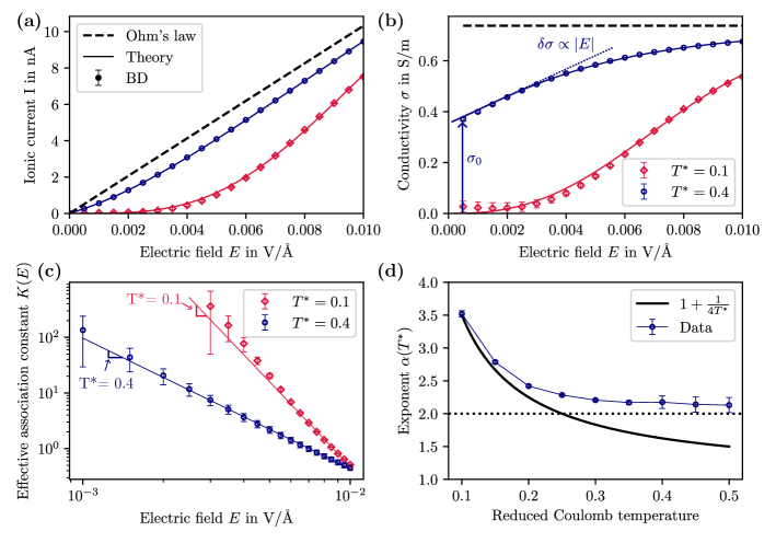
Figure 5: Comparison between BD transport simulations and theory. (a-b) Ionic current (a) and conductivity (b) for reduced Coulomb temperature of 0.1 (red) and 0.4 (blue), compared with Ohm’s law (dashed black line). Symbols: BD simulations. Solid lines: Theoretical model, Equation (84). (c) Symbols: Effective association constant $K(E)$ computed from the free ion fraction at various electric field, for a reduced Coulomb temperature $T^{*}$ of 0.1 (red) and 0.4 (blue). Solid lines: power-law fit, allowing to determine the value of the exponent $\beta$. (d) Symbols: Exponent $\alpha$ defined by the non-linearity in the IV curve, $j(E)\propto|E|^{\alpha}$, obtained from $\beta$ through $\alpha=1-\frac{\beta}{2}$. Black solid line: Theoretical prediction of the 2D Wien effect, see Equation (86). Dotted line: bulk exponent $\alpha=2$, obtained through Onsager’s theory of the Wien effect Onsager (1934).

III.2 Determination of the exponent at low field

In order to study the response of the system, it is easier to define an effective association constant $K(E)$ through:

$$K(E)=\frac{n_{p}(E)}{\delta n_{f}(E)^{2}}=\frac{1-n_{f}(E)}{\left(n_{f}(E)-n_{f}(0)\right)^{2}}.$$ (50)

In Figure 5.c, we plot the effective association constant as a function of the electric field. We observe that the curves are well approximated by a power law of the external field, with an exponent $\beta$ that we obtain by fitting the curve of $K(E)$ with $E$ in logarithmic scale (Fig. 5c). At small field, we have:

$$\delta j(E)\underset{E\to 0}{\propto}\frac{E}{{\sqrt{K(|E|)}}},$$ (51)

hence the current also follows a power law with the external field. The absolute value underlines the fact that the effective association constant - and then the conductivity - is symmetric under field inversion. We can thus define the exponent $\alpha(T^{*})$ of the power law:

$$\delta j(E)\underset{E\to 0}{\propto}{E\times|E|^{\alpha(T^{*})-1}},$$ (52)

which is, as expected, antisymmetric under field inversion. This exponent can be extracted from the slope from Figure 5.c, as $\alpha=1-\beta/2$. We find that this exponent strongly depends on temperature: we plot the evolution of $\alpha$ with the reduced Coulomb temperature in Figure 5.d. We observe that the value of the exponent depends on conditions (such as the strength of the interactions), which strongly contrasts with the original second Wien effect, which predicts an universal exponent of 2 for the transport of weak electrolyte regardless of details of interaction. We seem to recover this limit when the interaction between the ion becomes weak $T^{*}\to 1$ (blue curve in Figure 5.b). Surprisingly, the exponent drastically changes at a value close to the critical temperature, echoing the transition defined at equilibrium.

We checked that this exponent only depends on the strength of the interaction and not other interaction parameters, such as the short-distance cut-off $C$. The exponent obtained from our BD simulations is also in agreement with the exponents obtained in previous NEMD simulations of the system Robin, Kavokine, and Bocquet (2021).

III.3 Theory

In this section, we derive analytically the expression of the non-universal exponent $\alpha(T^{*})$. Our approach is based on an extension of Onsager’s study of the second Wien effect for bulk 3D weak electrolytes Onsager (1934). The generalization to 2D has been first developed in Ref. Robin, Kavokine, and Bocquet (2021) and we elaborate on this descritpion here to compare with our numerical results. In what follows, we restrict ourselves to the case of the ideal 2D Coulomb gas ($\xi=\infty$), and focus on the paired regime, ($T^{*}<T^{*}_{c}$).

III.3.1 An Onsager’s approach of the 2D Wien effect

We assume that the fraction $n_{f}$ follows a generic evolution equation, introducing a dissociation (resp. association) constant $\tau_{d}$ (resp. $\tau_{a}$):

$$\dot{n}_{f}=\frac{1-n_{f}}{\tau_{d}}-\frac{n_{f}^{2}}{\tau_{a}}.$$ (53)

At thermal equilibrium (in the absence of external field), the ratio of these to constants is given by $e^{2\mu_{e}}$, as discussed in the previous section. When driven out of equilibrium however, these two quantities may depend on the applied electric field $\boldsymbol{\mathrm{E}}=E\,\boldsymbol{\mathrm{\hat{x}}}$ acting along $x$.

Onsager showed that it is possible to link both $\tau_{a}$ and $\tau_{d}$ to the anion-cation correlation function $g$. Assuming that a cation is held fixed at the origin, $g(r,\theta)$ is the probability density of finding a negative ion at polar position $(r,\theta)$. It follows a Smoluchowski equation:

$$\partial_{t}g=2D\boldsymbol{\mathrm{\nabla}}\cdot(\boldsymbol{\mathrm{\nabla}}g+g\boldsymbol{\mathrm{\nabla}}V),$$ (54)

where $V$ is the total (dimensionless) electrostatic potential at $(r,\theta)$. It reads:

$$V=\frac{1}{T^{*}}\log\frac{r}{r_{0}}-\frac{r\cos\theta}{\ell_{E}}.$$ (55)

The first term of the potential corresponds to the unscreened interaction of two ions in confinement. This assumption is valid if the system is sufficiently paired up ($T^{*}<T^{*}_{c}$) so that the influence of other free ions can be neglected. Quantitatively, the Debye length $\lambda_{\text{D}}$ diverges if the system is fully paired, and therefore is not a relevant length scale. The second term corresponds to the external field, characterized by the following length scale:

$$\ell_{E}=\frac{k_{B}T}{Ze{|E|}}.$$ (56)

The potential $V$ has a maximum for $r\sim\ell_{E}/T^{*}$; a pair can be expected to break if its two ions are separated by a larger distance. This fixes the typical length scale of correlations in presence of the field.

Assuming the system has reached a steady state, we obtain:

$$\left[\Delta+\left(\frac{1}{T^{*}r}-\frac{\cos\theta}{\ell_{E}}\right)\partial_{r}+\frac{\sin\theta}{r\ell_{E}}\partial_{\theta}\right]g=0.$$ (57)

We then perform the change of variable $\boldsymbol{\mathrm{r}}\to\boldsymbol{\mathrm{u}}=\boldsymbol{\mathrm{r}}/\ell_{E}$:

$$\left[\Delta+\left(\frac{1}{T^{*}u}-\cos\theta\right)\partial_{u}+\frac{\sin\theta}{u}\partial_{\theta}\right]g=0.$$ (58)

This shows that the problem is scale invariant, as it is now entirely determined by a single dimensionless parameter $T^{*}$; this property is unique to the 2D geometry (where the Bjerrum length is infinite). Onsager’s trick consist in splitting the correlation function into two parts:

$$g=g_{d}+g_{a},$$ (59)

where $g_{d}$ and $g_{a}$ are two solutions of (58) associated with a source or a sink of particles at the origin, respectively:

$$\int_{0}^{2\pi}-2D\left[\boldsymbol{\mathrm{\nabla}}g_{a}+g_{a}\boldsymbol{\mathrm{\nabla}}V\right]\cdot\boldsymbol{\mathrm{\hat{r}}}\,r\mathrm{d}\theta=-C,$$ (60)

$$\lim\limits_{r\to\infty}g_{a}=\rho,$$ (61)

and

$$\int_{0}^{2\pi}-2D\left[\boldsymbol{\mathrm{\nabla}}g_{d}+g_{d}\boldsymbol{\mathrm{\nabla}}V\right]\cdot\boldsymbol{\mathrm{\hat{r}}}\,r\mathrm{d}\theta=+C,$$ (62)

$$\lim\limits_{r\to\infty}g_{d}=0,$$ (63)

where $C$ is a positive constant independent of $r$. In other words, $g_{a}$ describes a background of free ions recombining with the central ion to form new pairs, and $g_{d}$ pairs that break under the electric field. These two functions will allow us to compute $\tau_{a}$ and $\tau_{d}$.

Since any constant is a solution of the Smoluchowski equation, it is easy to see from the boundary condition that:

$$g_{a}=\rho,$$ (64)

and straightforward integration yields:

$$C=\frac{4\pi D\rho}{T^{*}}.$$ (65)

This is a recombination rate, defining the pair association time:

$$\tau_{a}=\frac{T^{*}}{4\pi D\rho}.$$ (66)

Interestingly, we find that the formation time of pairs is independent of the electric field. This result is general and is also valid in the bulk (but not in 1D), as recombination of freely diffusive ions is an uncorrelated process.

Onsager’s original approach to compute $g_{d}$, which involves an arduous expansion in terms of special functions, strongly relied on a fact that the 3D Smoluchowski equation is spatially separable; it fails in our 2D case. Instead, we exploit the fact that the 2D Smoluchowski equation is scale-invariant, and show how all relevant quantities can be computed up to a geometrical factor.

III.3.2 Self-similarity of the correlation function

We start be noticing that another solution of the Smoluchowski equation (58) is the Boltzmann distribution:

$$g_{0}(u,\theta)=\exp\left[-\frac{1}{T^{*}}\ln\frac{u\ell_{E}}{r_{0}}+u\cos\theta\right].$$ (67)

This is not the correct solution of the problem however, as the Boltzmann distribution only makes sense at thermal equilibrium. In particular, it does not verify the correct boundary conditions at $r\to\infty$. However, for $u\ll 1$ the external field is negligible compared to the field created by the central ion and pairs are in quasi-equilibrium (ions are strongly correlated and remain bounded over long timescales). Therefore, we admit that $g_{d}$ is the unique solution of the following problem:

$$\left[\Delta+\left(\frac{1}{T^{*}u}-\cos\theta\right)\partial_{u}+\frac{\sin\theta}{u}\partial_{\theta}\right]g_{d}=0,$$ (68)

$$g_{d}\sim K_{a}\left(\frac{\ell_{E}}{r_{0}}\right)^{-1/T^{*}}u^{-1/T^{*}}\ \text{for}\ u\to 0,$$ (69)

$$\lim\limits_{u\to\infty}g_{d}(u)=0,$$ (70)

where $K_{a}$ is a constant determined by the fact that the flux of $g_{d}$ should be equal to $+C$. The solution to this problem is unique because $g_{d}$ is known on the whole boundary of the domain. $\ell_{E}$ now only appears in a boundary condition at $u=0$, and the system is linear, so $g_{d}$ is fully determined from a single scaling function:

$$g_{d}(u)=K_{a}\left(\frac{l_{E}}{r_{0}}\right)^{-1/T^{*}}G(u),$$ (71)

where $G$ is a function that depends only on $T^{*}$. The balance between the fluxes of $g_{d}$ and $g_{a}$ reads:

$$2DK_{a}\left(\frac{\ell_{E}}{r_{0}}\right)^{-1/T^{*}}\mathcal{F}=\frac{4\pi D\rho}{T^{*}},$$ (72)

where $\mathcal{F}$ is the flux of the function $G$:

$$\mathcal{F}=-\int_{0}^{2\pi}\left[\boldsymbol{\mathrm{\nabla}}G+G\boldsymbol{\mathrm{\nabla}}\hat{V}\right]\cdot\boldsymbol{\mathrm{\hat{u}}}\,u\mathrm{d}\theta,$$ (73)

where the dimensionless potential $\hat{V}$ is given by:

$$\hat{V}=\frac{1}{T^{*}}\log u-u\cos\theta.$$ (74)

The flux $\mathcal{F}$ has the dimension of an inverse length squared and is independent of $\ell_{E}$ or $\rho$, since it describes a single pair breaking event. As the only remaining length-scale in the problem is $r_{0}$, we have (up to a geometrical factor):

$$\mathcal{F}\simeq r_{0}^{-2}.$$ (75)

We obtain the association constant $K_{a}$:

$$K_{a}=2\pi\left(\frac{\ell_{E}}{r_{0}}\right)^{1/T^{*}}\frac{\rho r_{0}^{2}}{T^{*}}=\frac{\tau_{d}}{\tau_{a}},$$ (76)

and the dissociation time $\tau_{d}$:

$$\tau_{d}=\frac{r_{0}^{2}}{2D}\left(\frac{\ell_{E}}{r_{0}}\right)^{1/T^{*}}.$$ (77)

In the steady state, the free ion fraction $n_{f}$ is given by Equation (53):

$$n_{f}=\frac{\tau_{a}}{2\tau_{d}}\left(\sqrt{1+\frac{4\tau_{d}}{\tau_{a}}}-1\right).$$ (78)

Assuming each free ion contributes linearly to conduction, we obtain the ionic current due to the Wien effect:

$$j(E)\propto{E\times|E|^{1/2T^{*}}}.$$ (79)

This predicts there that the ionic conductivity scales sublinearly with the temperature, as $\sigma\sim|E|^{1/2T^{*}}$. While this prediction reproduces qualitatively the non-linearity observed in the simulations, it typically underestimates the conductivity of the system by more than one order of magnitude. In particular, we do not find the exponent measured in the simulations.

In the next section, in order to explain this this behavior, we now take into account the formation of larger ionic clusters in presence of an external field.

III.3.3 Ionic clusters and anisotropic correlations

In the above derivation, the key assumption was the divergence of the Debye length $\lambda_{\text{D}}$, so that the problem becomes self-similar. We recall that $\lambda_{\text{D}}\propto n_{f}^{-1/2}$, and we found that $n_{f}\propto E^{1/2T^{*}}$, so that $\lambda_{\text{D}}\propto E^{-1/4T^{*}}$. If $T^{*}<1/4$, then $\lambda_{\text{D}}\gg\ell_{E}$ for all relevant values of the electric field, since $\ell_{E}\propto E^{-1}$.

This scaling argument seemingly validates our approach of considering that $\ell_{E}$ sets the scale of all correlations between ions. However, this argument only makes the sense when considering correlations along the $x$ axis: ions separated by more than $\ell_{E}$ are carried away by the electric field, so correlations on larger scale may be neglected. This is not the case, however, along the $y$ axis, so actually one should not neglect the influence of $\lambda_{\text{D}}$ on the problem: correlations are anisotropic.

The above analysis can be supported qualitatively by analyzing simulation results. In Brownian dynamics, we observe that ions tend to form elongated clusters in the direction of the electric field. Ions are able to move within these clusters, but remain within them for long times (see Figure S3). This suggests that the mobility of ions in the direction $x$ of the electric field may increase with the field strength, while diffusion in the orthogonal direction $y$ remains constrained by electrostatic correlations.

Taking anisotropic correlations into account, however, requires to account for many-body interactions in the Smoluchowski equation for $g$, which makes the problem intractable. Instead, we use a scaling argument, that we now detail.

Let us start by recovering the previous result using scaling laws. Equation (77) can be recast as an Arrhenius law:

$$\tau_{d}=\tau_{\text{diffusion}}\exp\left[-2\beta\Delta F\right]=\frac{r_{0}^{2}}{2D}\left(\frac{\ell_{E}}{r_{0}}\right)^{1/T^{*}},$$ (80)

where $\Delta F$ is the “free energy barrier” to break a pair. It reads:

$$\beta\Delta F\simeq-\frac{\log\ell_{E}/r_{0}}{2T^{*}}.$$ (81)

This argument is not fully rigorous, as the problem is far from equilibrium and this energy barrier strongly depends on an out-of-equilibrium quantity (the length scale $\ell_{E}$). However, this last expression is identical, upon replacing $\ell_{E}$ by $\lambda_{\text{D}}$ to the (properly defined) free energy cost of breaking a pair at equilibrium, given by Equation (36). We thus find that the kinetic energy barrier to break a pair is similar to the thermodynamic energy gap between the paired and the unpaired states, if we admit that the typical size of the ionic atmosphere in presence of an external field is given by $\ell_{E}$ instead of the Debye length $\lambda_{\text{D}}$.

Let us now use this simple argument to account for anisotropic correlations. Since the typical size of the correlation cloud of is $\ell_{E}$ along the $x$ axis and $\lambda_{\text{D}}$ along the $y$ axis, one may roughly approximate its overall spatial extension as $\ell=\sqrt{\lambda_{\text{D}}\ell_{E}}$. In this case, the free energy barrier to breaking a pair should read:

$$\beta\Delta F\simeq-\frac{\log\ell_{E}/r_{0}}{4T^{*}}-\frac{\log\lambda_{\text{D}}/r_{0}}{4T^{*}},$$ (82)

so that it is now the sum of two terms, corresponding to the energy barrier that an ion has to overcome to escape a cluster in the $x$ or $y$ direction, respectively. Conduction in the direction of the field is therefore associated with the Arrhenius timescale corresponding to the first term in the free energy:

$$\tau_{d,x}=\frac{r_{0}^{2}}{2D}\left(\frac{\ell_{E}}{r_{0}}\right)^{1/2T^{*}},$$ (83)

and we can define the proportion $n_{x}$ of ions that can freely move along the $x$ axis. It follows a evolution equation similar to Equation (37), with $\tau_{d,x}$ replacing $\tau_{d}$. We obtain:

$$n_{x}=\frac{\tau_{a}}{2\tau_{d,x}}\left(\sqrt{1+\left(\frac{2\tau_{d,x}}{\tau_{a}}\right)^{2}}-1\right)\underset{E\to 0}{\propto}E^{1/4T^{*}}.$$ (84)

We finally obtain the following prediction for the total ionic current:

$$j(E)\propto E\times n_{x}(E)\propto{E\times|E|^{\alpha(T^{*})-1}},$$ (85)

with

$$\alpha(T^{*})=1+\frac{1}{4T^{*}}.$$ (86)

III.3.4 Comparison with simulations and discussion

The comparison between our BD simulations and Equation (85) is plotted in Figure 5.a and b. Below the Kosterlitz-Thouless transition, the agreement is quantitative and the observed exponent $\alpha(T^{*})$ in simulations matches the theoretical prediction:

$$\boxed{\text{For }T^{*}<T_{c},\quad\sigma(E)\propto|E|^{1/4T^{*}},\quad\alpha\simeq 1+\frac{1}{4T^{*}}.}$$ (87)

Interestingly, this exponent is non-universal as it strongly depends on temperature; this contrasts with bulk electrolytes where the second Wien effect results in a universal conducivity increment scaling like $\delta\sigma\propto|E|$

Above the pairing transition, however, we observe deviations to the law. We find that the conductivity increases linearly with the applied field (Fig. 5b), which echoes the bulk Wien effect as mentioned above. We now suggest a possible explanation.

The key element in the above derivation that lead to the non-universal exponent $1/4T^{*}$ was the self-similarity of the correlation function. Below the KT transition, this assumption is valid as almost all ions are paired up, resulting in a diverging correlation function for electrostatic correlations: $\lambda_{\text{D}}\to\infty$. However, for $T^{*}>T_{c}$, some free ions remain even for $E=0$, and $\lambda_{\text{D}}$ always remains finite. Therefore, the correlation function is not self-similar as the problem now possesses two typical lengthscales: $\lambda_{\text{D}}$ and $\ell_{E}$. The second Wien effect may then be obtained from scaling laws: in absence of field, an ion pair breaks when its two ions are separated by more than $\lambda_{\text{D}}$ (after which they cease to interact). Under an electric field, this transition state between pairs and free ions is destabilized by roughly a factor $\lambda_{\text{D}}/\ell_{E}\propto|E|$. Since the dissociation timescale is approximatively the Arrhenius time associated with this intermediate state, conductivity also increases by a factor linear in $|E|$: we recover the scaling of Onsager’s Wien effect in bulk electrolytes. We therefore obtain:

$$\boxed{\text{For }T^{*}>T_{c},\quad\sigma(E)-\sigma(0)\propto|E|,\quad\alpha\simeq 2,}$$ (88)

in good agreement with numerical simulations (Fig. 5b).

It should be noted, however, that in the bulk, the remaining free ions at $E=0$ do not play a significant role at sufficient dilution, because $\lambda_{\text{D}}>\ell_{\text{B}}$ and so correlations still have a typical length scale $\ell_{\text{B}}$. In other words, the conductivity increment will scale like $E$ at all temperatures and does not directly depends on ion concentration, unlike in confined electrolytes.

The above derivation was performed assuming that all ions are paired up. In what follows, we account for ions that remain free even in absence of any field by adding a contribution $n_{f}(0)$ to the above result; this term is determined by the procedure described in Section II.2.1. The above sections were dedicated to the theoretical analysis of the 2D Wien effect at low temperature ($T^{*}<T^{*}_{c}$). We find that the conductivity of 2D confined electrolytes evolves as a power law of the electric field, with a non-universal exponent $1/4T^{*}$. This contrasts with the 3D bulk case, where the Wien exponent is 1.

Lastly, we note that in both cases $T^{*}>T_{c}$ and $T^{*}<T_{c}$ the exponent cannot be found through simple symmetry arguments, which would dictate that $\sigma\propto E^{2}$ (as the system is invariant by reversing the direction of the electric field). This originates in the fact that the correlation function $g$ becomes strongly polarized in the direction of the field, breaking the $x\to-x$ symmetry. In the bulk case, the conductivity increment scales like the ratio $\ell_{\text{B}}/\ell_{E}\propto E$, with $\ell_{\text{B}}$ the Bjerrum length. Since this quantity is infinite in 2D, the problem becomes self-similar and the increment is found to scale like a non-universal power law.

Conclusion

In this paper, we investigate the effect of long range electrostatic correlations on the equilibrium and transport of ions confined in a 2D slit. We use a combination of molecular dynamics simulations, analytical theory and Brownian dynamics (where water and channel walls are treated implicitly, and ion-ion interactions are renormalized). In all cases, we find that 2D confinement results in stronger electrostatic interactions, leading to the formation of ionic pairs. We showed that this phenomenon is associated to a phase transition analogous to the Kosterlitz-Thouless transition, and suppresses linear ionic conduction at low temperature.

In addition, the application of an external field can result in the breaking of ion pairs and in an increase in conduction. This process, known as the Wien effect, leads to strongly non-linear ion transport under confinement.

We expect that the effective potential approach used in this paper could be extended to explore other materialsKavokine, Robin, and Bocquet (2022), but also other geometries, for example the case of multiple ionic layersCoquinot et al. (2024), by changing the effective interaction potential accordingly.

Overall, we obtain excellent agreement between our analytical models and numerical results, for both the pairing transition and the 2nd Wien effect. In particular, we find that in the pair-dominated regime, the ionic current behaves like a power law of the applied field, with a non-universal exponent that can be predicted from analytical field theories. This regime, where the conductivity strongly vanishes at low electric field, can be considered as ionic coulomb blockade situation – although no gating dependence is considered here –.

This work is also a further demonstration of the very particular nature of electrostatic interactions in confined geometry. The strong ionic correlations gives rise to a complex variety of structures and behaviours, but the large-scale picture remains unaffected and can be adequately understood in term of a small set of parameters. Consequently, this work sheds light on the structure of ion-ion correlations in confined systems, and on the ionic dynamics of nanofluific in general.

Finally, the emergence of strongly non-linear conduction effects in 2D is a richness which can be exploited to develop nanofluidic systems with advanced properties, such as memristors Robin et al. (2022); Robin and Bocquet (2023). This is an opportunity which will certainly result in further developments in this active domain Kamsma et al. (2024); Emmerich et al. (2024); Paulo et al. (2023)

References

- Bocquet and Charlaix (2010) L. Bocquet and E. Charlaix, “Nanofluidics, from Bulk to Interfaces,” Chem. Soc. Rev. 39, 1073–1095 (2010).
- Garaj et al. (2010) S. Garaj, W. Hubbard, A. Reina, J. Kong, D. Branton, and J. A. Golovchenko, “Graphene as a Subnanometre Trans-Electrode Membrane,” Nature 467, 190–193 (2010).
- Lee et al. (2010) C. Y. Lee, W. Choi, J.-H. Han, and M. S. Strano, “Coherence Resonance in a Single-Walled Carbon Nanotube Ion Channel,” Science 329, 1320–1324 (2010).
- Feng et al. (2016) J. Feng, M. Graf, K. Liu, D. Ovchinnikov, D. Dumcenco, M. Heiranian, V. Nandigana, N. R. Aluru, A. Kis, and A. Radenovic, “Single-Layer MoS2 Nanopores as Nanopower Generators,” Nature 536, 197–200 (2016).
- Secchi et al. (2016) E. Secchi, S. Marbach, A. Niguès, D. Stein, A. Siria, and L. Bocquet, “Massive Radius-Dependent Flow Slippage in Carbon Nanotubes,” Nature 537, 210–213 (2016).
- Radha et al. (2016) B. Radha, A. Esfandiar, F. C. Wang, A. P. Rooney, K. Gopinadhan, A. Keerthi, A. Mishchenko, A. Janardanan, P. Blake, L. Fumagalli, M. Lozada-Hidalgo, S. Garaj, S. J. Haigh, I. V. Grigorieva, H. A. Wu, and A. K. Geim, “Molecular Transport through Capillaries Made with Atomic-Scale Precision,” Nature 538, 222–225 (2016).
- Esfandiar et al. (2017) A. Esfandiar, B. Radha, F. C. Wang, Q. Yang, S. Hu, S. Garaj, R. R. Nair, A. K. Geim, and K. Gopinadhan, “Size Effect in Ion Transport through Angstrom-Scale Slits,” Science 358, 511–513 (2017).
- Kavokine, Netz, and Bocquet (2021) N. Kavokine, R. R. Netz, and L. Bocquet, “Fluids at the Nanoscale: From Continuum to Subcontinuum Transport,” Annual Review of Fluid Mechanics 53, 377–410 (2021).
- Kavokine et al. (2019) N. Kavokine, S. Marbach, A. Siria, and L. Bocquet, “Ionic Coulomb Blockade as a Fractional Wien Effect,” Nature Nanotechnology 14, 573–578 (2019).
- Kavokine, Robin, and Bocquet (2022) N. Kavokine, P. Robin, and L. Bocquet, “Interaction Confinement and Electronic Screening in Two-Dimensional Nanofluidic Channels,” The Journal of Chemical Physics 157, 114703 (2022).
- Robin and Bocquet (2023) P. Robin and L. Bocquet, “Nanofluidics at the Crossroads,” The Journal of Chemical Physics 158, 160901 (2023).
- Richards et al. (2012) L. A. Richards, A. I. Schäfer, B. S. Richards, and B. Corry, “The Importance of Dehydration in Determining Ion Transport in Narrow Pores,” Small 8, 1701–1709 (2012).
- Robin et al. (2022) P. Robin, T. Emmerich, A. Ismail, A. Niguès, Y. You, G.-H. Nam, A. Keerthi, A. Siria, A. K. Geim, B. Radha, and L. Bocquet, “Long-Term Memory and Synapse-like Dynamics of Ionic Carriers in Two-Dimensional Nanofluidic Channels,” (2022), issue: arXiv:2205.07653 _eprint: 2205.07653.
- Robin, Kavokine, and Bocquet (2021) P. Robin, N. Kavokine, and L. Bocquet, “Modeling of Emergent Memory and Voltage Spiking in Ionic Transport through Angstrom-Scale Slits,” Science 373, 687–691 (2021).
- Emmerich et al. (2022) T. Emmerich, K. S. Vasu, A. Niguès, A. Keerthi, B. Radha, A. Siria, and L. Bocquet, “Enhanced Nanofluidic Transport in Activated Carbon Nanoconduits,” Nature Materials 21, 696–702 (2022).
- Levin (2002) Y. Levin, “Electrostatic Correlations: From Plasma to Biology,” Reports on Progress in Physics 65, 1577–1632 (2002).
- Minnhagen (1987) P. Minnhagen, “The Two-Dimensional Coulomb Gas, Vortex Unbinding, and Superfluid-Superconducting Films,” Reviews of Modern Physics 59, 1001–1066 (1987).
- Robin et al. (2023) P. Robin, A. Delahais, L. Bocquet, and N. Kavokine, “Ion filling of a one-dimensional nanofluidic channel in the interaction confinement regime,” The Journal of Chemical Physics 158 (2023), publisher: AIP Publishing.
- Zhao et al. (2021) W. Zhao, Y. Sun, W. Zhu, J. Jiang, X. Zhao, D. Lin, W. Xu, X. Duan, J. S. Francisco, and X. C. Zeng, “Two-Dimensional Monolayer Salt Nanostructures Can Spontaneously Aggregate Rather than Dissolve in Dilute Aqueous Solutions,” Nature Communications 12, 5602 (2021).
- Fong et al. (2024) K. Fong, B. Sumic, N. O’Neill, C. Schran, C. Grey, and A. Michaelides, “The Interplay of Solvation and Polarization Effects on Ion Pairing in Nanoconfined Electrolytes,” Preprint (Chemistry, 2024).
- Avni et al. (2022) Y. Avni, R. M. Adar, D. Andelman, and H. Orland, “Conductivity of concentrated electrolytes,” Physical Review Letters 128, 098002 (2022).
- Abraham et al. (2024) M. Abraham, A. Alekseenko, V. Basov, C. Bergh, E. Briand, A. Brown, M. Doijade, G. Fiorin, S. Fleischmann, S. Gorelov, G. Gouaillardet, A. Grey, M. E. Irrgang, F. Jalalypour, J. Jordan, C. Kutzner, J. A. Lemkul, M. Lundborg, P. Merz, V. Miletic, D. Morozov, J. Nabet, S. Pall, A. Pasquadibisceglie, M. Pellegrino, H. Santuz, R. Schulz, T. Shugaeva, A. Shvetsov, A. Villa, S. Wingbermuehle, B. Hess, and E. Lindahl, “GROMACS 2024.1 Manual,” (2024), 10.5281/ZENODO.10721192.
- Thompson et al. (2022) A. P. Thompson, H. M. Aktulga, R. Berger, D. S. Bolintineanu, W. M. Brown, P. S. Crozier, P. J. In ’T Veld, A. Kohlmeyer, S. G. Moore, T. D. Nguyen, R. Shan, M. J. Stevens, J. Tranchida, C. Trott, and S. J. Plimpton, “LAMMPS - a Flexible Simulation Tool for Particle-Based Materials Modeling at the Atomic, Meso, and Continuum Scales,” Computer Physics Communications 271, 108171 (2022).
- Gowers et al. (2016) R. Gowers, M. Linke, J. Barnoud, T. Reddy, M. Melo, S. Seyler, J. Domański, D. Dotson, S. Buchoux, I. Kenney, and O. Beckstein, “MDAnalysis: A Python Package for the Rapid Analysis of Molecular Dynamics Simulations,” in Python in Science Conference (Austin, Texas, 2016) pp. 98–105.
- Stukowski (2010) A. Stukowski, “Visualization and Analysis of Atomistic Simulation Data with OVITO–the Open Visualization Tool,” Modelling and Simulation in Materials Science and Engineering 18, 015012 (2010).
- Hagberg, Swart, and Schult (2008) A. Hagberg, P. J. Swart, and D. A. Schult, “Exploring network structure, dynamics, and function using networkx,” (2008).
- Berendsen, Grigera, and Straatsma (1987) H. J. C. Berendsen, J. R. Grigera, and T. P. Straatsma, “The Missing Term in Effective Pair Potentials,” The Journal of Physical Chemistry 91, 6269–6271 (1987).
- Ryckaert, Ciccotti, and Berendsen (1977) J.-P. Ryckaert, G. Ciccotti, and H. J. Berendsen, “Numerical Integration of the Cartesian Equations of Motion of a System with Constraints: Molecular Dynamics of n-Alkanes,” Journal of Computational Physics 23, 327–341 (1977).
- Darden, York, and Pedersen (1993) T. Darden, D. York, and L. Pedersen, “Particle Mesh Ewald: An \emphN \cdotlog( \emphN ) Method for Ewald Sums in Large Systems,” The Journal of Chemical Physics 98, 10089–10092 (1993).
- Essmann et al. (1995) U. Essmann, L. Perera, M. L. Berkowitz, T. Darden, H. Lee, and L. G. Pedersen, “A Smooth Particle Mesh Ewald Method,” The Journal of Chemical Physics 103, 8577–8593 (1995).
- Swope et al. (1982) W. C. Swope, H. C. Andersen, P. H. Berens, and K. R. Wilson, “A Computer Simulation Method for the Calculation of Equilibrium Constants for the Formation of Physical Clusters of Molecules: Application to Small Water Clusters,” The Journal of Chemical Physics 76, 637–649 (1982).
- Bussi, Donadio, and Parrinello (2007) G. Bussi, D. Donadio, and M. Parrinello, “Canonical Sampling through Velocity Rescaling,” The Journal of Chemical Physics 126, 014101 (2007).
- Schlaich, Knapp, and Netz (2016) A. Schlaich, E. W. Knapp, and R. R. Netz, “Water Dielectric Effects in Planar Confinement,” Physical Review Letters 117, 048001 (2016).
- Fumagalli et al. (2018) L. Fumagalli, A. Esfandiar, R. Fabregas, S. Hu, P. Ares, A. Janardanan, Q. Yang, B. Radha, T. Taniguchi, K. Watanabe, G. Gomila, K. S. Novoselov, and A. K. Geim, “Anomalously Low Dielectric Constant of Confined Water,” Science 360, 1339–1342 (2018).
- Bjerrum (1926) N. Bjerrum, Untersuchungen Über Ionenassoziation. I. Der Einfluss Der Ionenassoziation Auf Die Aktivität Der Ionen Bei Mittleren Assoziationsgraden, von Niels Bjerrum (B. Lunos, 1926).
- Kaiser (2014) V. Kaiser, The Wien Effect in Electric and Magnetic Coulomb Systems - from Electrolytes to Spin Ice, Theses, Ecole normale superieure de lyon - ENS LYON (2014).
- Onsager (1934) L. Onsager, “Deviations from Ohm’s Law in Weak Electrolytes,” The Journal of Chemical Physics 2, 599–615 (1934).
- Kaiser et al. (2013) V. Kaiser, S. T. Bramwell, P. C. W. Holdsworth, and R. Moessner, “Onsager’s Wien effect on a lattice,” Nature Materials 12, 1033–1037 (2013).
- Berthoumieux, Démery, and Maggs (2024) H. Berthoumieux, V. Démery, and A. C. Maggs, “Non-monotonic conductivity of aqueous electrolytes: beyond the first Wien effect,” (2024), version Number: 1.
- Kosterlitz and Thouless (1973) J. M. Kosterlitz and D. J. Thouless, “Ordering, Metastability and Phase Transitions in Two-Dimensional Systems,” Journal of Physics C: Solid State Physics 6, 1181–1203 (1973).
- Rotenberg, Bernard, and Hansen (2018) B. Rotenberg, O. Bernard, and J.-P. Hansen, “Underscreening in Ionic Liquids: A First Principles Analysis,” Journal of Physics: Condensed Matter 30, 054005 (2018).
- Coquinot et al. (2024) B. Coquinot, M. Becker, R. R. Netz, L. Bocquet, and N. Kavokine, “Collective modes and quantum effects in two-dimensional nanofluidic channels,” Faraday Discussions 249, 162–180 (2024).
- Kamsma et al. (2024) T. M. Kamsma, J. Kim, K. Kim, W. Q. Boon, C. Spitoni, J. Park, and R. van Roij, “Brain-inspired computing with fluidic iontronic nanochannels,” Proceedings of the National Academy of Sciences 121, e2320242121 (2024).
- Emmerich et al. (2024) T. Emmerich, Y. Teng, N. Ronceray, E. Lopriore, R. Chiesa, A. Chernev, V. Artemov, M. Di Ventra, A. Kis, and A. Radenovic, “Nanofluidic logic with mechano–ionic memristive switches,” Nature Electronics 7, 271–278 (2024).
- Paulo et al. (2023) G. Paulo, K. Sun, G. Di Muccio, A. Gubbiotti, B. Morozzo della Rocca, J. Geng, G. Maglia, M. Chinappi, and A. Giacomello, “Hydrophobically gated memristive nanopores for neuromorphic applications,” Nature Communications 14, 8390 (2023).