Interplay between external driving, dissipation and collective effects in the Markovian and non-Markovian regimes

Abstract

The evolution of quantum optical systems is determined by three key factors: the interactions with their surrounding environment, externally controlled lasers and between the different system components. Understanding the interplay between the three dynamical contributions is essential for the study of out-of-equilibrium phenomena as well as technological applications. The present study investigates open system phenomena in driven optical systems coupled simultaneously to a bosonic field. For a linear system of micro-cavities coupled to a photonic crystal, it is analytically shown that environmental interaction and external control cause significant non-Markovian corrections to the applied coherent drive. Additionally, collective cross-driving effects arise when multiple modes are coupled to the same field, where a laser applied to one mode effectively drives other modes. Based on the linear solution, a non-Markovian master equation for two-level emitters is derived. Remarkably, the proposed equation of motion remains accurate even for moderate driving intensities, where emitters cannot be approximated by bosonic modes. The influence of the non-linearity is analyzed and benchmarked against an exact pseudo-mode solution, and compared with established master equations in the Markovian regime. Within this regime, the comparison demonstrates the presence of short-time non-Markovian effects at times well beyond the inverse of the environment’s bandwidth, and memory effects induced by short laser pulses. These findings offer valuable insights into the driven open system dynamics of quantum optical systems, impurities embedded in solid-state materials, molecular systems, and more, paving the way for precise control of their quantum states.

I Introduction

The framework of driven open quantum systems describes the evolution of a broad range of physical systems Breuer and Petruccione (2002); Weiss (2012); Carmichael (1999); Rivas and Huelga (2012). Examples range from free electrons Gorlach et al. (2023) and single atoms Mabuchi and Doherty (2002); Walther et al. (2006); Hamsen et al. (2017) to defects in bulk materials Schirhagl et al. (2014); Liu et al. (2019) and many-body systems Bloch et al. (2008); Diehl et al. (2008); Zeiher et al. (2016); Sieberer et al. (2016); Bluvstein et al. (2021). The dynamics of these systems is simultaneously influenced by externally controlled fields, denoted as “drive” or “control”, and the inevitable interaction with their surrounding environment.

The many-body nature of these composite systems and the large number of timescales involved in the evolution restrict the number accurate solutions and limit perturbative analysis to specific physical regimes. The presence of the coherent drive introduces further theoretical difficulties in the evaluation of the primary system’s reduced dynamics. The drive is commonly represented by an explicit time-dependent term in the Hamiltonian, which breaks time-translation symmetry and formally necessitates a time-ordering procedure.

Under typical circumstances, the reduced dynamics of the open system are deduced by relying on a weak coupling with the environment and rapid decay of environmental correlations Breuer and Petruccione (2002); Cohen-Tannoudji et al. (1998), leading to a Markovian description. Nevertheless, with the introduction of structured environments, such as photonic crystals John (1987); John and Quang (1994); Goban et al. (2014); Joannopoulos et al. (1997) and nanophotonic structures Douglas et al. (2015); Chang et al. (2018), moderate system-environment coupling Prior et al. (2010); Matsuzaki et al. (2011); Chin et al. (2012); Huelga and Plenio (2013); Esposito et al. (2015), and increasingly short laser pulses, a theoretical treatment beyond the Markovian regime is required Rivas et al. (2014); Breuer et al. (2016); De Vega and Alonso (2017). A comprehensive dynamical description is essential for both the analysis of natural processes such as energy transport in biological light harvesting complexes Blankenship et al. (2011); Huelga and Plenio (2013), and electron-phonon interactions Holstein (1959); Hubbard (1964), as well as in the development of quantum control tools Rebentrost et al. (2009); Goban et al. (2014); Koch (2016), single-photon sources Arcari et al. (2014); Hood et al. (2016), sensing Chin et al. (2012); Matsuzaki et al. (2011), and information processing techniques Gonzalez-Tudela et al. (2011); Hung et al. (2016).

The present contribution employs an analytical construction of a non-Markovian master equation to investigate the dynamics of linear and non-linear driven open quantum systems. We focus on drive-dependent phenomena and highlight the intricate interplay between coherent driving, dissipation and memory and effects.

Non-Markovian dynamics of driven non-linear open systems have been studied extensively using a variety of numerical techniques. Quasi-adiabatic Makri and Makarov (1995); Sahrapour and Makri (2013) and non-interacting/inter-blip path integral methods Leggett et al. (1987); Grifoni et al. (1995); Winterstetter and Weiss (1997), hierarchical equations of motion Meier and Tannor (1999); Jin et al. (2008); Wang and Chen (2013); Xu and Ankerhold (2023), generalized master equations Grifoni et al. (1996); Magazzù et al. (2018), renormalization group methods Shapourian (2016), driven Liouville von-Neumann formalism Hod et al. (2016) and stochastic Schrödinger equation Orth et al. (2013) have been employed to study the non-Markovian dynamics of various systems. Specifically, a large effort has been devoted to the analysis of the spin-boson model, which serves as a toy model for chemical processes involving two isolated quantum states coupled to a complex environment such as a solvent, molecular vibrations, or protein scaffolds Leggett et al. (1987); Weiss (2012).

The numerical methods are often both precise and efficient in a defined physical regime, such as moderate temperature or up to second order in the system-environment coupling strength. Moreover, they compute system expectation values. Importantly, even when the dynamics of the expectation values can be evaluated accurately, it remains extremely difficult to differentiate and analyze the underlying dominant physical processes. This information is readily obtained by analyzing the form of an analytical equation of motion, where the role of different terms can be traced to distinct physical process.

Notably, Ref. Amati (2024) employed a numerical solution of the hierarchical equations of motion to investigate signatures of non-Markovianity in the periodically driven spin-boson model. These include negativity in the decay rates of a time-local master equation and memory kernel decay time of a generalized Lindblad master equation. Alternatively, previously proposed analytical approaches for non-linear systems have relied on either the slow variation of the spectral density Cao et al. (2021), or a high driving frequencies Grifoni et al. (1996); Hartmann et al. (2000).

The dynamics of Non-driven open linear systems have been studied extensively Caldeira and Leggett (1983); Unruh and Zurek (1989); Hu et al. (1992); Lambropoulos et al. (2000); Xiong et al. (2010); Wu et al. (2010); Zhang et al. (2012), while driven systems have been studied in the context of bosonic Lei and Zhang (2012) and fermionic Tu and Zhang (2008) transport models, coherent control Quang et al. (1997) and the derivation of an exact master equation Yang et al. (2013).

In the Markovian regime, neglecting information backflow from the environment greatly simplifies the problem. Nevertheless, even within this regime, the interplay between the coherent and incoherent dynamical contributions is not fully understood. It is well known that the interaction with the environment leads to coherent dynamical contributions in the form of Lamb shifts Lamb Jr and Retherford (1947); Hänsch et al. (1975); Röhlsberger et al. (2010); Meir et al. (2014), and dispersive forces Dung et al. (2002); Buhmann (2013); González-Tudela et al. (2015). However, the reverse effect, where the coherent drive modifies the dissipation, requires further investigation. Previous analysis focusing on different driving regimes predict distinct conclusions Scully and Zubairy (1999); Szczygielski et al. (2013); Albash et al. (2012); Dann et al. (2018). Determining the effect of coherent driving on the dissipation has direct implications for the development of open system control techniques Khodjasteh et al. (2010); Koch (2016); Dann et al. (2019, 2020); Kuperman et al. (2020); Dupays et al. (2020); Dupays and Chenu (2021), noise mitigation Cai et al. (2023), and the engineering of effective coherent dynamics in the presence of external noise Kallush et al. (2022); Aroch et al. (2024).

To gain further insight and address these issues, we study the driven Markovian and non-Markovian dynamics of two simple classes of optical open systems: (a) A linear system of coupled modes and (b) a collection of two level-emitters coupled to a bosonic environment. In this context the term “linear system” refers to a bosonic system with a quadratic composite Hamiltonian, such that the dynamics can be described by a compact operator algebra. As a consequence, the dynamics of such a composite system can be expressed by a set of linear coupled differential equations, where the number of equations corresponds to the number of harmonic modes. In comparison, for a non-linear system, such as a two-level emitter coupled to bosonic modes, the composite operator algebra is non-compact, leading to an infinite set of coupled linear differential equations even for a single environment mode Bruus and Flensberg (2004).

We begin by analyzing the dynamics of a linear open system in Sec. III. Within the rotating wave approximation, the standard quantum optics Hamiltonian conserves the number of excitations (U(1) symmetry). In this case, the reduced dynamics of a linear primary system can be expressed in terms of a time-local non-Markovian master equation of the Kossakowski form Lei and Zhang (2012); Zhang et al. (2012); Yang et al. (2013). In this form, the jump operators are time-independent, while decay rates and Lamb shifts of the exact master equation vary in time and are completely determined by the so-called Keldysh non-equilibrium Green function and the Bose-Einstein distribution.

We apply the resolvent formalism Cohen-Tannoudji et al. (1998); Economou (2006); González-Tudela and Cirac (2017) to evaluate the Green function for a simplified model of a 1D photonic crystal Goban et al. (2014); Lodahl et al. (2015); González-Tudela and Cirac (2017). When the emitter-environment coupling is comparable to the Bloch band’s width, such a model enables probing highly non-Markovian dynamics, which require non-perturbative approaches, and explores the interplay between bound states and coherent driving. The implications of the master equation are analyzed in Sec. III. Interestingly, for a linear system, the normalized frequencies and decay rates depend only on the environment’s properties, implying the dissipation and drive are independent. We find that the coherent drive manifests a non-Markovian self-correction, modifying the Hamiltonian driving term, Sec. III.4. By employing the resolvant formalism, the magnitude of the non-Markovian driving term is related to distinct features of the self energy and the environmet’s spectrum. When multiple linear modes are coupled to the same bosonic non-Markovian environment, it leads to cross-driving terms, where a laser applied to one mode drives other modes, Sec. III.5.

Beyond the rotating wave approximation one obtains a general quadratic Hamiltonian (breaking the U(1) symmetry). Extending the construction of Ferialdi Ferialdi (2016), it is shown in Sec. III.2 that the structure of the master equation maintains the same form as in the case where the number of excitations is conserved. Namely, the dissipation remains independent of the drive.

Building upon the analytical solution of the linear driven open system an equation of motion for a system of quantum emitters is constructed in Sec. IV.2. Motivated by the clear connection, the governing dynamical equation is coined as the Linear Master Equation (LME). Intuitively, the construction is based on the assumption that the environment’s influence on the primary system is only negligibly affected by the non-linearity. A priori, such an approach is expected to remain valid in the low excitation regime where the non-linearities of the emitters play a minor role Porras and Cirac (2008). Benchmarking the proposed solution against an exact pseudo-mode solution demonstrates that the LME remains accurate even in the presence of a moderate drive, where the two-level system transition is saturated. Moreover, it provides a good approximation for strong system-environment coupling, where memory effects play a dominant role. Surprisingly, in such a non-Markovian regime (and for a non-linear primary system) it is not even clear that the reduced dynamics can be described in terms of a time-local master equation Nakajima (1958); Zwanzig (1960); Shibata et al. (1977); Chaturvedi and Shibata (1979); Hall et al. (2014); Breuer and Petruccione (2002); De Vega and Alonso (2017).

The dynamical description in terms of a simple master equation allows an intuitive differentiation of the simultaneously occurring dynamical processes. These involve an interplay between coherence, dissipation, and backflow of information.

The pseudo-mode simulation technique constitutes an alternative approach by which to solve the non-Markovian dynamics Garraway (1997a). Specifically, for a bosonic environment initially in a Gaussian state, the exact reduced dynamics can be mapped to the same system coupled to a reservoir constructed from a finite number of dissipative bosonic pseudo-modes, undergoing Markovian decay Garraway (1997a); Tamascelli et al. (2018). The substitution of an environment with an infinite number of modes by a finite-mode dissipative reservoir reduces the numerical cost of solving the reduced system dynamics. It enables a well-controlled truncation of the infinite Hilbert space. Here, we emphasize that mapping to pseudo-modes also holds for driven systems and apply the construction to study the non-Markovian effects of driven open quantum systems, Sec. IV.1. We consider the simplest case of a Lorentzian spectral density, which requires only a single dissipative pseudo-mode. Such a model is equivalent to an atomic system trapped in a dissipative cavity Walther et al. (2006); Blais et al. (2021).

The underlying dynamical processes are analyzed by comparing the exact solution to the predictions of the LME and its Markovian limit, the Optical Bloch Master Equation (OBE) Scully and Zubairy (1999), Sec. IV. In the short-time regime ($t<0.5/\Gamma_{FGR}$) the LME typically achieves orders of magnitude improvement in accuracy relative to the OBE, even for strong driving. Here, $\Gamma_{FGR}$ is the Markovian decay rate, given by the Fermi-golden rule. Surprisingly, this result demonstrates that the non-Markovian effects may provide a significant contribution to the dynamics for time durations much larger than the environment’s memory time. For weak driving, the accuracy typically exhibits a minimum value around $t=1/\Gamma_{FGR}$ and increases for longer times reaching a comparable (but typically lower) accuracy relative to the OBE. Increasing the driving strength and non-Markovianity typically leads to larger deviations from the exact result. This arises from the enhanced likelihood of reabsorbing the emitted photon along with the system’s non-linearity.

In the extremely non-Markovian driving regime, where the laser pulse (drive) and the environment’s bandwidth are comparable, novel non-Markovian effects emerge, Sec. IV.4. In light of rapid technological advancements in pulse engineering, and contemporary efforts to reduce inevitable dissipation losses by minimizing the duration of the driving protocols, such non-Markovian effects may significantly reduce gate fidelities if not accounted for.

To illuminate the extent of interplay between the dissipative and coherent dynamical contributions in the Markovian regime, the exact evolution is compared to common Markovian theoretical treatments for a monochromatic drive and Gaussian pulse, Sec. IV.6. We compare the performance of the LME and OBE to the Floquet Ho et al. (1986); Kohler et al. (1997); Breuer and Petruccione (1997); Chu and Telnov (2004); Szczygielski et al. (2013); Szczygielski (2014), Adiabatic Albash et al. (2012), and Time-dependent Di Meglio et al. (2023) master equations. These dynamical equations typically differ by the associated driving regime and the transition between states of a certain basis that capture the dissipation process. Unlike the LME and OBE, where the environment induces transition between the bare system states, the three other constructions incorporate the drive within the dissipation process. They are based on the dressed basis approach Cohen-Tannoudji et al. (1998), Floquet and adiabatic theorems, leading to representation of the open system dynamics in terms of transitions between different preferred basis states and drive-dependent decay rates.

In the studied parameter range, the Linear and Optical Bloch master equations exhibit excellent agreement with the exact solution, while the drive-dependent approaches show significant relative deviations. Surprisingly, this trend occurs even for very strong driving, where the dressed-state picture is the natural framework to analyze the dynamics. This counterintuitive result highlights the importance of comparison to exact models or simulations even in the regime, where all the assumptions of the microscopic derivations are valid.

Finally, we emphasize that the present work focuses on optical systems interacting with the electromagnetic field. For such setups, it is well justified to consider a bosonic environment at $T=0$. Nevertheless, all the results can be generalized to the case of $T>0$ in a straightforward manner; see the discussion section and Appendix A.1. In addition, a similar theoretical analyses applies for a wide range of physical systems, such as solid-state color centers interacting with lattice phonon modes Doherty et al. (2013); Goldman et al. (2015), molecular electronic or spin states coupled to molecular or solvent vibrational modes Pachón and Brumer (2011); Ishizaki and Fleming (2012) and many more Lodahl et al. (2015); Blais et al. (2021); Barreiro et al. (2011); Wang et al. (2024); Byczuk and Vollhardt (2008); Anders et al. (2010); Strand et al. (2015); Scarlatella et al. (2021).

II Framework

We consider a driven open quantum system coupled to a bosonic environment. The evolution of the composite system is generated by the Hamiltonian

$$H=H_{S}\left({t}\right)+H_{I}+H_{E}\leavevmode\nobreak\ \leavevmode\nobreak\ .$$ (1)

Here, the system Hamiltonian includes the bare system and drive terms $H_{S}\left({t}\right)=H_{S0}+H_{d}\left({t}\right)$, $H_{I}$ describes the system-environment interaction and $H_{E}$ is the bare environment Hamiltonian. $\hbar$ is taken to be unity throughout the paper.

The explicit time-dependent representation of the drive can be obtained from an autonomous (time-independent) description by an interaction picture transformation of an initially coherent field state Cohen-Tannoudji et al. (1998), . As a result, the explicit time-dependent non-Markovian description remains precise even for a weak coherent drive and includes both the influence of the field’s quantum fluctuations and the system’s back action on the field. The representation of the drive in terms of an explicit time-dependent term is valid in the non-relativistic regime and moderate field intensities, for which the particles-field interaction energy is negligible relative to the free particle energy . Alternatively, the validity is maintained as long as the Rabi frequency is much smaller than the system’s typical frequency. Within this parameter regime, each explicitly time-dependent Hamiltonian can be mapped to a corresponding autonomous Hamiltonian with a modified initial state.

The nature of the reduced dynamics is determined by the relation between a restricted number of characteristic energy scales: (a) the typical frequency of the system $\omega_{S}$, (b) detuning with respect to the central laser frequency $\Delta=\omega_{S}-\omega_{L}$, (c) driving bandwidth $\Delta\omega_{L}$, (d) environment spectral width $\Delta\omega_{E}$, (e) inverse of the local density of environment states $1/D\left({\omega_{S}}\right)$, as well as (f) the system-environment coupling $g_{SE}$, and (g) the system-drive coupling $g_{SL}$. Additional factors which influence the dynamical behavior are the interplay between the light polarization and the spatial dimensions of the medium Lodahl et al. (2017) and retardation effects Sinha et al. (2020). Since the present focus concerns the dynamical effects of the drive, these considerations are neglected.

A number of dynamical regimes can be identified. Markovian evolution emerges when the environment’s spectral features change on a scale much larger than the system’s transition linewidth, i.e.,

$$g_{SE}^{2}D\left({\omega_{S}}\right)\ll\Delta\omega_{E}\leavevmode\nobreak\ \leavevmode\nobreak\ .$$ (2)

This leads to memoryless dynamics, where information backflow can be neglected, and the dissipation is characterized by an exponential decay with a rate given by Fermi’s Golden Rule (FGR) $\Gamma_{\text{FGR}}\sim g_{SE}^{2}D\left({\omega_{S}}\right)$.

For a pulsed control protocol, the introduction of a new dynamical variable, the pulse’s bandwidth $\Delta\omega_{L}$, leads to further richness in the dynamical behavior. When the bandwidth of the pulse is comparable to $\Delta\omega_{E}$, information backflow modifies the system’s reduced dynamics. These non-Markovian effects may occur even when the Markovian condition (Eq. (2)) is satisfied.

Beyond the Markovian regime, the restriction given by (2) is lifted, and the system evolution may exhibit information backflow, resulting in oscillatory behavior Rivas et al. (2014), power-law decay rates Wódkiewicz and Eberly (1976); Knight (1978) and strong dispersive interactions González-Tudela and Cirac (2017). Additionally, bound system-environment states may appear, leading to fractional decay and localized light states John (1987); John and Wang (1990); Yablonovitch (1987); Bykov (1975); Kurizki (1990); Shi et al. (2016); González-Tudela and Cirac (2017).

In the extreme non-Markovian regime, where $g_{SE}>\Delta\omega_{E}$, the impact of information backflow surpasses the dynamical contribution of the dissipative processes. As a consequence, the abstract partition of the composite system into a primary system and environment breaks down. This qualitative transition motivates the inclusion of dominant environmental modes within the so-called primary system Jang et al. (2008).

In most of the current study, we focus on system-environment Hamiltonians which conserve the number of excitations (usually derived by a rotating wave approximation). For such composite systems, it is convenient to work a frame rotating at the central laser frequency $\omega_{L}\approx\omega_{S}$. The rotation amount to shifting the spectrum of the system and environment and adding oscillating phases to the drive. As a consequence, the open system dynamics are not influenced by the magnitude of $\omega_{S}$, which constitutes only a reference frequency in the studied class of models. The validity conditions of the rotating wave approximation and the mapping of an autonomous Hamiltonian to an explicitly time-dependent one coincide.

III Linear optical systems

We first consider a linear system of $N_{S}$ coupled resonators with frequencies $\omega_{1},\omega_{2},\dots,\omega_{N_{S}}$ interacting with a bosonic field initially in the vacuum state. Physical realizations of the theoretical model include driven coupled micro-resonators Hajjaj et al. (2020), mechanical oscillators Jost et al. (2009); Kotler et al. (2021) and nano-structured photonic materials Lodahl et al. (2015). The latter constitutes an especially attractive platform, where high controllability enables access to exotic dynamical regimes involving strong system-environment couplings, a high density of states and narrow environmental bandwidths. For further experimental considerations see Sec. V.

Within the rotating wave approximation, the composite linear system Hamiltonian takes the following form

$$H=\sum_{ij}M_{ij}a^{\dagger}_{i}a_{j}+\sum_{i}\left({f_{i}\left({t}\right)a_{i}^{\dagger}+f_{i}^{*}\left({t}\right)a_{i}}\right)\\ \sum_{k,i}\left({\eta_{ik}a^{\dagger}_{i}b_{k}+\eta_{ik}^{*}a_{i}b_{k}^{\dagger}}\right)+\sum_{k}\omega_{k}b_{k}^{\dagger}b_{k}\leavevmode\nobreak\ \leavevmode\nobreak\ ,$$ (3)

where $a_{i}$ and $b_{k}$ are system and environment annihilation operators, with $i,j=1,\dots,N_{S}$, and $k=1,\dots,N_{E}$, $k$ may account for both the mode’s wavevector and polarization. The first two terms represent the internal system couplings and drive, while the last terms corresepond to the system-environment interaction and the free environment Hamiltonian, respectively. The following analysis considers bosonic modes; nevertheless, it applies as well to fermionic Hamiltonians of the form of (3) with minor modifications, Appendix A.1.

Before pursuing the exact system dynamics, it is beneficial to establish the connection between the Hamiltonian parameters and the typical energy scales. The typical system energy scale, $\omega_{S}$, is associated with the characteristic magnitude of the eigenvalues of $\bm{M}$, while the environment’s bandwidth, $\Delta\omega_{E}$, is given by the variance of $\omega_{k}$ in the continuum limit. $g_{SL}\sim|f_{i}\left({t}\right)|$, while $\Delta\omega_{L}$ is defined as the typical standard deviation of the driving terms $\{f_{i}\left({t}\right)\}$ Fourier transform, and $g_{SE}$ corresponds to the ratio of the spectral density and the density of states $g_{SE}^{2}\sim\sum_{k}|\eta_{ik}|^{2}\delta\left({\omega-\omega_{k}}\right)/D\left({\omega_{S}}\right)$.

III.1 Exact master equation

The master equation for a driven bosonic composite systems, whose evolution is governed by a quadratic Hamiltonian was derived in Zhang et al. (2012) (detailed derivations and an extension to fermionic composite systems is given in Yang et al. (2013)). The construction employs a coherent state representation, which can be evaluated analytically for a quadratic Hamiltonian of the form (3). An exact Fokker-Planck equation for dynamical propagator is then deduced and mapped to a time-convolution-less master equation. It is explicitly given by

$$\dot{\rho}_{S}\left({t}\right)=-i\left[{\tilde{H}_{S}\left({t}\right),\rho_{S}\left({t}\right)}\right]\\ +\sum_{ij}\Gamma_{ij}^{\downarrow}\left({t}\right){\cal D}_{a_{j},a_{i}^{\dagger}}\left[{\rho_{S}\left({t}\right)}\right]+\Gamma_{ij}^{\uparrow}\left({t}\right){\cal D}_{a_{i}^{\dagger},a_{j}}\left[{\rho_{S}\left({t}\right)}\right]\leavevmode\nobreak\ \leavevmode\nobreak\ ,$$ (4)

where ${\cal D}_{x,y}\left[{\bullet}\right]\equiv x\bullet y-\{yx,\bullet\}/2$, with

$$\tilde{H}_{S}\left({t}\right)=\sum_{ij}a^{\dagger}_{i}{\Omega}_{ij}\left({t}\right)a_{j}+\sum_{i}\left({k_{i}\left({t}\right)a_{i}^{\dagger}+k_{i}^{*}\left({t}\right)a_{i}}\right)\leavevmode\nobreak\ \leavevmode\nobreak\ .$$ (5)

Here the relaxation rates $\Gamma_{ij}^{\downarrow}$ and $\Gamma_{ij}^{\uparrow}$, and coherent term $\Omega_{ij}$, given explicitly in Appendix A.1, are determined by the time-dependent matrix elements of the Keldysh non-equilibrium Green function $\bm{W}\left({t,0}\right)$ Schwinger (1961). The Green function is an $N_{S}$ by $N_{S}$ matrix that satisfies the integro-differential equation

$$\dot{\bm{W}}\left({t,t^{\prime}}\right)+i\bm{M}\bm{W}\left({t,t^{\prime}}\right)+\int_{t^{\prime}}^{t}{d\tau\bm{K}\left({t-\tau}\right)\bm{W}\left({\tau,t^{\prime}}\right)=0}\leavevmode\nobreak\ \leavevmode\nobreak\ ,$$ (6)

with initial condition $\bm{W}\left({0,0}\right)=\bm{I}_{S}$, where $M_{ij}$ are elements of $\bm{M}$, $\bm{K}\left({t,t^{\prime}}\right)=\bm{K}\left({\tau=t-t^{\prime}}\right)=\int_{0}^{\infty}{d\omega\bm{J}\left({\omega}\right)e^{-i\omega\tau}}$ is the memory kernel and the elements of the spectral density functions read $\left[{\bm{J}}\right]_{jk}=\sum_{l}\eta_{jl}\eta_{kl}^{*}\delta\left({\omega-\omega_{l}}\right)$. The drive terms $\{k_{i}\}$ are elements of the vector

$$\bm{k}\left({t}\right)=\bm{f}\left({t}\right)+\bm{f}_{NM}\left({t}\right)$$ (7)

with

$$\bm{f}_{NM}\left({t}\right)=\int_{0}^{t}{\dot{\bm{W}}\left({t,\tau}\right)\bm{f}\left({\tau}\right)d\tau}-\dot{\bm{W}}\bm{W}^{-1}\tilde{\bm{f}}\leavevmode\nobreak\ \leavevmode\nobreak\ ,$$ (8)

where $\dot{x}\equiv dx/dt$, $\tilde{\bm{f}}\left({t}\right)=\int_{0}^{t}{\bm{W}\left({t,\tau}\right)\bm{f}\left({\tau}\right)d\tau}$, and the elements of the vector $\bm{f}\left({t}\right)$ are the corresponding driving terms, $\{f_{i}\}$, of Eq. (3).

The form of the master equation, (4), highlights three phenomena arising from the system-environment interaction: (i) The interaction modifies the primary system’s coherent dynamics by effectively coupling different system modes, manifested by the non-diagonal terms of $\bm{\Omega}$ , (ii) it leads to the emergence of a drive-dependent coherent term $\bm{f}_{NM}$, Eq. (7). For multiple system modes, the non-Markovian correction may lead to a collective effect, where cross-mode coupling elements in $\bm{W}$ imply that an effective drive on the $i$’th mode $k_{i}\left({t}\right)$ depends on the chosen driving protocols of the other modes $\{f_{j}\left({t}\right)\}$. This contribution is weighted in a non-local way by the spectral density function elements, as depicted by Eq. (8). (iii) Finally, the form of $\Gamma_{ij}^{\downarrow,\uparrow}$ highlights that for such a linear system, the incoherent decay rates are independent of the drive.

In the Markovian limit, the Green function obtains the form $\bm{W}\left({t}\right)=\exp\left({-i{\cal H}_{eff}t}\right)$, where ${\cal H}_{eff}$ is a constant non-Hermitian matrix (for example, see Subsec. III.3). Substituting the exponential form into Eq. (8) shows that $\bm{f}_{NM}$ vanishes in this regime. Thus, the cross-relation is a purely non-Markovian effect. In addition, it constitutes a non-Markovian signature, allowing to detect deviations from Markovianity by the analysis of the coherent dynamics of linear or weakly excited systems.

The non-Markovian contributions of $\bm{f}_{NM}\left({t}\right)$ scale quadratically with the system-environment coupling. Hence, such a collective driving effect is expected to be significant only for strong system environment-coupling, where the open-system dynamics are highly non-Markovian. In the weak coupling regime, ignoring such open system contributions leads to small coherent errors. Nevertheless, with the ongoing improvement in coherent control and contemporary aspirations for precise control, even small errors may be significant. In order to optimize control fidelity the coherent collective-driving effects can be incorporated in the design of control protocols.

Finally, the autonomous representation of the composite system, where the dynamics are generated by a time-independent composite Hamiltonian with an environment initially in a multi-mode coherent state Cohen-Tannoudji et al. (1998), highlights that the source of the coherent correction, $\bm{f}_{NM}$, is the initial environment state. Such non-Markovianity is quite exotic, as memory effects commonly arise solely from the spectral features of the environment and strong system-environment interaction. A similar effect has been witnessed in the non-Markovian evolution of a fermonic open system Windt et al. (2024). It is important to highlight that $\bm{f}_{NM}$ differs qualitatively from the Lamb shift correction to the bare frequencies. The latter originates from the exchange of virtual photons, while the former is associated with the presence of real photons in the field Lamb Jr and Retherford (1947); Hänsch et al. (1975).

III.2 Beyond the rotating wave approximation

The standard derivation of $H$, Eq. (3), involves canonical quantization of the analogous classical system. This procedure leads to counter rotating terms proportional to $a_{i}b_{k}$ and $a_{i}^{\dagger}b_{k}^{\dagger}$ Cohen-Tannoudji et al. (1997). In the optical regime and typical system-environment coupling, these terms contribute rapid fluctuations on the order of the coupling, and are, therefore commonly neglected. Nevertheless, they are essential for the accurate computation of Lamb shifts, dispersive forces and entanglement dynamics Fleming et al. (2010). Moreover, for strong coupling, the counter rotating terms modify the reduced dynamics substantially Zueco et al. (2009); Agarwal et al. (2012).

The presence of counter rotating terms in the composite Hamiltonian breaks the U(1) symmetry of the Hamiltonian in the autonomous representation. Naturally, the reduction in symmetry increases the complexity of the calculation of the reduced system dynamics. In the following section we study the structure of the master equation for an initial Gaussian state of the environment and arbitrary quadratic Hamiltonian. For such an initial state, a generalization of Ref. Ferialdi (2016) leads to the general form. The result highlights that the same qualitative interplay between the drive and dissipation, as deduced in Sec. III.1, is maintained beyond the rotating wave approximation.

The exact non-Markovian master equation, governing the dynamics of a non-driven linear (bosonic) system, coupled to a bosonic environment by a bi-linear interaction term was derived in Ref. Ferialdi (2016). In contrast to the previous section, here a general linear coupling is considered: $H_{I}=\sum_{j}S^{j}E_{j}$, where $S^{j}$ and $E_{j}$ are linear combinations of the system and environment creation/annihilation operators, respectively. We employ the covariant contravariant like notation in the present section to simplify the presentation .

The construction presented in Ref. Ferialdi (2016) starts from the most general completely positive, trace preserving Gaussian map Diósi and Ferialdi (2014). By exploiting the initial Gaussian state of the environment and Wick’s theorem Wick (1950), Ferialdi deduced the exact dynamical generator of the reduced system. In the Schrödinger picture the generator obtains the form

$$\frac{d}{dt}\rho_{S}\left({t}\right)=-i\left[{H_{S0},\bullet}\right]+{\cal L}^{\text{lin}}\left[{\rho_{S}\left({t}\right)}\right]\leavevmode\nobreak\ \leavevmode\nobreak\ ,$$ (9)

with

$${\cal L}^{\text{lin}}\left[{\bullet}\right]=\sum_{jk}\Gamma_{jk}\left({t}\right)\left[{S^{j},\left[{S^{k},\bullet}\right]}\right]\\ +\Theta_{jk}\left({t}\right)\left[{S^{j}\left[{\dot{S}^{k},\bullet}\right]}\right]-i\Sigma_{jk}\left({t}\right)\left[{S^{j},\{S^{k},\bullet\}}\right]\\ -i\Upsilon_{jk}\left({t}\right)\left[{S^{j}\{\dot{S}^{k},\bullet\}}\right]\leavevmode\nobreak\ \leavevmode\nobreak\ .$$ (10)

Here, $H_{S0}$ is an arbitrary time-independent bosonic quadratic system Hamiltonian, governing the isolated (non-driven) system dynamics. The decay rates: $\Gamma_{jk}$, $\Theta_{jk}$, $\Sigma_{jk}$ and $\Upsilon_{jk}$ include convolutions over memory kernels ${\cal A}_{jk}\left({t}\right)$, and ${\cal B}_{jk}\left({t}\right)$, and propagators of the free system ${\cal C}_{k}^{j}\left({t-s}\right)$ and $\tilde{\cal C}_{k}^{j}\left({t-s}\right)$, see Appendix B for explicit expressions. The propagators of the (non-driven) linear system relate Heisenberg picture operators at different times

$$S^{j}\left({s_{1}}\right)=\sum_{k}{\cal C}_{k}^{j}\left({t-s_{1}}\right)S^{k}\left({t}\right)+\tilde{\cal{C}}_{k}^{j}\left({t-s_{1}}\right)\dot{S}^{k}\left({t}\right)\leavevmode\nobreak\ \leavevmode\nobreak\ .$$ (11)

After introducing known results, we next incorporate the influence of a linear drive on the open system dynamics. Consider the following system Hamiltonian

$$H_{S}^{\prime}\left({t}\right)=H_{S0}+H_{d}\left({t}\right)\leavevmode\nobreak\ \leavevmode\nobreak\ ,$$

where $H_{d}\left({t}\right)$ is a linear driving term (same form as in Eq. (3)). Transforming to an interaction picture relative to both bare dynamics and the drive (with respect to $H_{S}^{\prime}\left({t}\right)$) leads to a representation where the composite system dynamics are generated by the interaction picture Hamiltonian,

$$\tilde{H}_{I}\left({t}\right)=\sum_{j}\tilde{S}^{j}\left({t}\right)E_{j}\left({t}\right)\leavevmode\nobreak\ \leavevmode\nobreak\ .$$ (12)

This Hamiltonian is bi-linear in the system-environment bosonic operators and, without loss of generality, can be assumed to satisfy $\text{tr}_{E}\left({H_{I}\left({t}\right)}\right)=0$ Schaller (2014) . As a consequence, one can repeat the construction presented in Ref. Ferialdi (2016) with only minor modifications. Foremost, in the presence of a linear drive, the dynamics in the Heisenberg picture acquire an additional scalar term,

$$\tilde{S}^{j}\left({s_{1}}\right)=\sum_{k}{\cal C}_{k}^{j}\left({t-s_{1}}\right)S^{k}\left({t}\right)\\ +\tilde{\cal{C}}_{k}^{j}\left({t-s_{1}}\right)\dot{S}^{k}\left({t}\right)+\bar{{C}}^{j}\left({t-s_{1}}\right)\leavevmode\nobreak\ \leavevmode\nobreak\ ,$$ (13)

where the memory kernels ${\cal C}$ and $\tilde{\cal{C}}$ are identical to the non-driven case, Eq. (11). In Appendix B, we show that the modified Heisenberg dynamics, relative to Eq. (11), does not alter the resulting decay rates, $\Gamma$, $\Theta$, $\Sigma$ and $\Upsilon$. Its sole contribution is new coherent term in the master equation, similarly to Eq. (4).

Overall, we obtain general form

$$\frac{d}{dt}\rho_{S}\left({t}\right)=-i\left[{H^{\prime}_{S}\left({t}\right),\rho_{S}\left({t}\right)}\right]\\ -i\sum_{j}\Phi_{j}\left({t}\right)\left[{S^{j},\rho_{S}\left({t}\right)}\right]+{\cal L}^{\text{lin}}\left[{\rho_{S}\left({t}\right)}\right]\leavevmode\nobreak\ \leavevmode\nobreak\ ,$$ (14)

where $\Phi\left({t}\right)$ is given in Appendix B. This relation provides a more general expression than Eq. (4), as it generally includes the dynamical contributions of the counter rotating terms in the system-environment interaction. The downside is that the memory kernels, ${\cal{A}}_{jk}$ and ${\cal B}_{jk}$, are given in terms of asymptotic series of complex multidimensional integrals (similarly to the Dyson series). Hence, for practical calculations they require a perturbative analysis.

Importantly, the structure of Eq. (14) highlights that the inclusion of counter rotating terms does not change the qualitative interplay between coherent and incoherent dynamical contributions. Namely, the coherent drive does not affect the dissipation. Establishing this point, in the following analysis, we return to the case where the counter rotating terms have been neglected, leading to an autonomous Hamiltonian which conserves the number of excitations.

III.3 Exact dynamical solution

The evolution of the reduced system associated with $H$, Eq. (3), is determined by the non-equilibrium Green function $\bm{W}$. The Green function is determined by the integro-differential equation (6) which is independent of the driving terms. Obtaining analytical solutions to Eq. (6), is generally an elaborate task. In the case of a single system mode and certain memory kernels $\bm{K}$, a solution can be obtained by employing standard Laplace transform identities Vacchini and Breuer (2010). Beyond these cases, a general methodology applicable to multiple system modes and a broader class of environments is desirable. In the following section, we describe such an approach. By relying on the resolvent formalism Cohen-Tannoudji et al. (1998), the method provides a systematic way to obtain exact or approximate solutions for $\bm{W}\left({t}\right)\equiv\bm{W}\left({t,0}\right)$.

The non-driven system dynamics can be concisely expressed in terms of the Heisenberg equations of motion of the operator valued vector $\bm{v}\left({t}\right)=\{\bm{a}\left({t}\right),\bm{b}\left({t}\right)\}^{T}$, where $\bm{a}=\{a_{1}\dots,a_{N_{S}}\}^{T}$ and $\bm{b}=\{b_{1},\dots,b_{N_{E}}\}^{T}$, while the time-dependence designates operators in the Heisenberg picture. The composite system dynamics reduce to a Schrödinger-like equation

$$\dot{\bm{v}}\left({t}\right)=-i{\cal H}\bm{v}\left({t}\right)\leavevmode\nobreak\ \leavevmode\nobreak\ ,$$ (15)

where

$${\cal H}=\left[{\begin{array}[]{cc}\bm{M}&\bm{R}\\ \bm{R}^{\dagger}&\bm{E}\end{array}}\right]\leavevmode\nobreak\ \leavevmode\nobreak\ ,$$ (16)

with $\left[{\bm{R}}\right]_{il}=\eta_{il}$ and $\bm{E}=\text{diag}\left({\omega_{1},\dots,\omega_{N_{E}}}\right)$. Such representation motivates treating the annihilation operators as elements of an $N_{S}+N_{E}$-dimensional vector space.

The solution of Eq. (15) is equivalently stated in terms of the dynamical propagator ${\cal U}\left({t}\right)=\exp\left({-i{\cal H}t}\right)$. To obtain a solution for $\cal U$, it is beneficial to express the propagator in an integral form

$${\cal{U}}\left({t}\right)=-\frac{1}{2\pi i}\int_{-\infty}^{\infty}e^{-iEt}\bm{G}\left({E+i0^{+}}\right)dE\leavevmode\nobreak\ ,$$ (17)

where

$$\bm{G}\left({z}\right)=\frac{1}{z-{\cal H}}$$ (18)

is the resolvent. The correspondence between Eq. (17) and its standard exponential form can be shown by an analytical continuation of the integral to the complex plane and application of the residue theorem. The strength of the formalism stems from the form of Eq. (17), which enables employing complex contour integration techniques to evaluate the elements of $\cal U$. In addition, Eq. (17) circumvents the demanding task of exponentiating the large matrix ${\cal H}$, when the inverse, Eq. (18), can be accurately evaluated by alternative techniques.

The form of the propagator naturally decomposes to four block matrices

$${\cal U}=\left[{\begin{array}[]{cc}\bm{W}&\bm{T}\\ \bm{T}^{\dagger}&\bm{P}\end{array}}\right]\leavevmode\nobreak\ \leavevmode\nobreak\ ,$$ (19)

corresponding to the structure of the resolvent

$$\bm{G}\left({z}\right)=\left[{\begin{array}[]{cc}\bm{G}_{S}&\bm{G}_{SE}\\ \bm{G}_{SE}^{\dagger}&\bm{G}_{E}\end{array}}\right]\leavevmode\nobreak\ \leavevmode\nobreak\ ,$$ (20)

where $\bm{G}_{S}$ ($\bm{G}_{E}$) is a $N_{S}$ by $N_{S}$ ($N_{E}$ by $N_{E}$) matrix. The block inversion formula now leads to (see Appendix A.3)

$$\bm{G}_{S}\left({z}\right)=\bm{Q}\left({z}\right)$$

$$\bm{G}_{SE}\left({z}\right)=-\bm{Q}\left({z}\right)\bm{R}\frac{1}{z-\bm{E}}$$ (21)

$$\bm{G}_{E}\left({z}\right)=\frac{1}{z-\bm{E}}+\frac{1}{z-\bm{E}}\bm{R}^{\dagger}\bm{Q}\left({z}\right)\bm{R}\frac{1}{z-\bm{E}}\leavevmode\nobreak\ \leavevmode\nobreak\ ,$$

with

$$\bm{Q}\left({z}\right)=\left[{z-\bm{M}-\bm{\Sigma}\left({z}\right)}\right]^{-1}\leavevmode\nobreak\ \leavevmode\nobreak\ ,$$ (22)

where the self-energy is given by

$$\bm{\Sigma}\left({z}\right)=\bm{R}\frac{1}{z-\bm{E}}\bm{R}^{\dagger}\leavevmode\nobreak\ \leavevmode\nobreak\ .$$ (23)

Finally, by combining Eq. (17) , (19), (20), (21) and (22), the non-equilibrium Green function is expressed as

$$\bm{W}\left({t}\right)=-\frac{1}{2\pi i}\int_{-\infty}^{\infty}\frac{e^{-iEt}}{{E^{+}-\bm{M}-\bm{\Sigma}\left({E^{+}}\right)}}dE\leavevmode\nobreak\ ,$$ (24)

employing the notation $E^{+}=\lim_{\eta\rightarrow 0^{+}}E+i\eta$. Similarly, $\bm{T}$ and $\bm{P}$ can be expressed in an analogous form, in terms of $\bm{G}_{SE}$ and $\bm{G}_{E}$, respectively.

For certain environments analytical expressions for $\bm{\Sigma}$ can be computed analytically Economou (2006); Morita (1971); Katsura et al. (1971, 1971); Horiguchi and Chen (1974); Guttmann (2010), numerically Haydock et al. (1972); Haydock (1980); Viswanath and Müller (1994); Bulla et al. (1998); Pulci et al. (1998); Allerdt and Feiguin (2019) or perturbatively Cohen-Tannoudji et al. (1998). When an analytical expression for $\bm{\Sigma}$ is available, the integral of Eq. (24) can be solved by contour integration. The contour integral includes three types of contributions: (a) Real poles, which correspond to bound system-environment states (b) unstable complex poles that leading to dissipation and (c) branch cuts, which contribute a power-law decay. This analysis enables expressing the Green function as

$$\bm{W}\left({t}\right)=\sum_{\alpha\in SP}\bm{R}_{\beta}e^{-iz_{\alpha}t}+\sum_{\beta\in UP}\bm{R}_{\beta}e^{-iz_{\beta}}+\sum_{\gamma\in BC}C_{\gamma}\leavevmode\nobreak\ \leavevmode\nobreak\ ,$$ (25)

where $SB$ and $UP$ designates the set of stable poles and unstable poles, while $C_{\gamma}$ are the contributions of the contour segment circumventing the branch cuts.

In the Markovian limit, the weak system-environment coupling and smooth dependence of density of states on the energy allows approximating the self-energy by

$$\bm{\Sigma}\left({E+i0^{+}}\right)\approx\bm{\Sigma}\left({E_{0}+i0^{+}}\right)=\bm{\Delta}_{0}-i\bm{\Gamma}_{0}/2\leavevmode\nobreak\ \leavevmode\nobreak\ ,$$ (26)

where $E_{0}$ is taken as the average of system energies, while the elements of the Hermitian matrices $\bm{\Delta}_{0}$ and $\bm{\Gamma}_{0}$ include the collective Lamb shifts and decay rates, Appendix A.2. Such an approximation effectively includes the contribution of only a single pole to the solution of (17), neglecting the other poles and branch cuts. A straightforward application of the residue theorem now leads to the Markovian solution of the Green function

$$\bm{W}\left({t}\right)\approx\exp\left({-i{\cal H}_{eff}t}\right)\leavevmode\nobreak\ \leavevmode\nobreak\ \\$$ (27)

$${\cal H}_{eff}=\bm{M}+\bm{\Delta}_{0}-i\bm{\Gamma}_{0}/2\leavevmode\nobreak\ \leavevmode\nobreak\ .$$

Once $\bm{W}$ is obtained, exactly or approximately, the extension of the analysis to the case of a driven system is achieved by including an additional non-homogeneous term in Eq. (15). The linear non-homogeneous equation then admits the general dynamical solution

$$\bm{v}\left({t}\right)={\cal U}\left({t}\right)\bm{v}\left({0}\right)-i\int_{0}^{t}{\cal U}\left({t-s}\right)\tilde{\bm{f}}\left({s}\right)ds\leavevmode\nobreak\ \leavevmode\nobreak\ ,$$ (28)

where $\tilde{f}=\{\bm{f},\bm{0}\}^{T}$ is an $N_{S}+N_{E}$ size vector, containing the driving terms in its first $N_{S}$ elements. Relation Eq. (28) provides an exact solution for both the system and environment modes in the presence of a drive. The structure of the second term, and non-diagonal form of $\cal U$, highlights that the system and environment modes are generally affected by the drive.

These results conclude the first part of the analysis of linear systems. In the following section, we apply the general relations to study the dynamics of simple primary systems and demonstrate the drive related non-Markovian phenomena.

III.4 Single harmonic mode coupled to a 1D photonic crystal

We demonstrate the general dynamical solution by considering a minimal model describing a driven nano-cavity coupled to a 1D photonic crystal. The photonic crystal is modeled by a chain of $N_{E}$ identical bosonic modes, interacting by nearest-neighbour interactions, with periodic boundary conditions and initially in the vacuum state. The composite system Hamiltonian reads

$$H=\omega_{S}a^{\dagger}a+g\left({ab^{\dagger}_{0}+a^{\dagger}b_{0}}\right)+H_{E}^{\left({t.b}\right)}\leavevmode\nobreak\ \leavevmode\nobreak\ ,$$ (29)

where the photonic crystal is represented by a tight-binding model

$$H_{E}^{\left({t.b}\right)}=\omega_{E}\sum_{j\in\mathbb{Z}_{N_{E}}}b_{j}^{\dagger}b_{j}-J\sum_{j\in\mathbb{Z}_{N_{E}}}\left({b_{j}^{\dagger}b_{j+1}+b_{j+1}^{\dagger}b_{j}}\right)\leavevmode\nobreak\ \leavevmode\nobreak\ ,$$ (30)

and the nano-cavity is coupled to single environment site. The considered model may exhibit strong non-Markovian dynamics, and exotic phenomena as fractional and power-law decay González-Tudela and Cirac (2017) as well as system-environment bound states Leonforte et al. (2021); Shi et al. (2016), while allowing for an analytical dynamical solution.

The photonic crystal’s bare Hamiltonian can be diagonalized by introducing the Fourier transformed operators $b_{k}=\frac{1}{\sqrt{L}}\sum_{j}e^{-ikaj}b_{j}$, with lattice constant $a$ and $k\in\left({2\pi/L}\right)\mathbb{Z}_{N_{E}}$. The substitution leads to a band structure within the energy range $\left[{\omega_{E}-2J,\omega_{E}+2J}\right]$. In the rotating frame with respect to $\omega_{E}$, Eq. (30) can now be concisely expressed as

$$H=\bar{\Delta}a^{\dagger}a+g\left({ab_{k}^{\dagger}+a^{\dagger}b_{k}}\right)\\ +\sum_{k}\omega_{k}b_{k}^{\dagger}b_{k}\leavevmode\nobreak\ \leavevmode\nobreak\ ,$$ (31)

with $\bar{\Delta}=\omega_{S}-\omega_{E}$ The environment spectrum $\omega_{k}=-2J\cos\left({ka}\right)$ manifests diverging density of states at the band edges: $D\left({E}\right)=\frac{\theta\left({2J-E}\right)}{\pi\sqrt{4J^{2}-E^{2}}}$ Economou (2006). The rapid change in density of states leads to highly non-Markovian behavior when $|\bar{\Delta}|\approx 2J$ John and Wang (1990), see Fig. 2 Panel (b). Interestingly, such increase in the density of states results in an enhancement in the coupling efficiencies between the system mode and the photonic crystal, which can assist in the realization of single photon transistors, large single photon nonlinearities and creation of single photon sources Arcari et al. (2014).

The solutions for $\bm{W}$ and $\bm{T}$ follow a procedure similar to that presented in Ref. González-Tudela and Cirac (2017), studying the spontaneous emission of two-level emitters, coupled to a 1D and 2D cubic lattices. Here, we summarize the results and provide a detailed analysis in Appendix C.2. Following, we utilize these results to investigate the non-Markovian effects associated with the drive. Utilizing Eq. (28) it can be readily inferred that system dynamics obtains the form

$$a\left({t}\right)=W\left({t}\right)a\left({0}\right)+\bm{T}\left({t}\right)\bm{b}\left({0}\right)-i\int_{0}^{t}W\left({t-s}\right)f\left({s}\right)\leavevmode\nobreak\ \leavevmode\nobreak\ ,$$ (32)

where in this case the non-equilibrium Green function and the drive term are simply time-dependent scalars

$${W}\left({t}\right)=-\frac{1}{2\pi i}\int_{-\infty}^{\infty}\frac{e^{-iEt}}{{E^{+}-{\omega_{S}}-{\Sigma}_{1D}\left({E^{+}}\right)}}dE\leavevmode\nobreak\ ,$$ (33)

with the self energy

$$\Sigma_{1D}\left({z}\right)=\frac{\text{sign}{\left({\text{Re}\left({z}\right)}\right)}g^{2}}{\sqrt{z^{2}-4J^{2}}}\leavevmode\nobreak\ \leavevmode\nobreak\ .$$ (34)

Finally, the integrals of Eq. (33) (similarly for $\bm{T}$) are solved by contour integral techniques, González-Tudela and Cirac (2017) and Appendix C.1.

The non-driven dynamics ($f=0$) exhibit similar non-Markovian features as the single excitation case, described in González-Tudela and Cirac (2017). Fractional decay, for frequencies close to the band edge, arises from an initial overlap with bound states (real poles of $G_{S}\left({z}\right)$), and a $t^{-3}$ power-law decay due to the contributions of branch cuts to the integral Eq. (33).

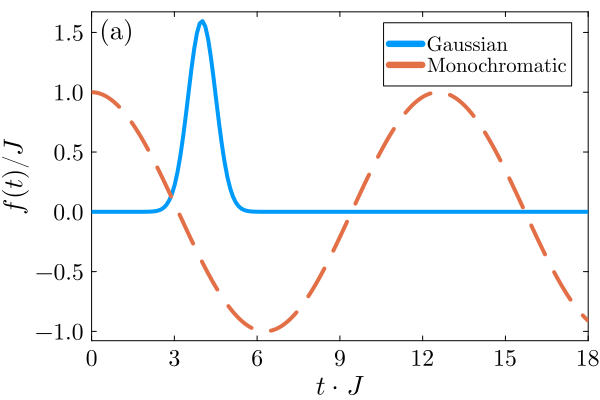
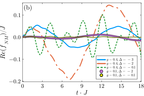
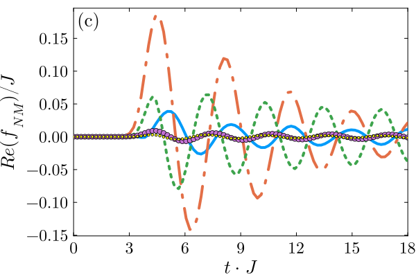
Figure 1: Non-Markovian influence of the drive. (a) Real part of the control protocols as a function of time. Two types of protocols are analyzed, an off resonant monochromatic drive (continuous blue) $f_{\text{mono}}\left({t}\right)=\exp\left({-i\left({\omega_{S}+\delta}\right)t}\right)$, with $\delta=0.5J$ and a Gaussian pulse $f_{\text{gauss}}=(A/\sqrt{2\pi\sigma^{2}})\left({-(t-t_{0})^{2}/2\sigma_{L}^{2}}\right)\exp\left({-i\omega_{S}t}\right)$. (b,c) The non-Markovian drive dependent coherent correction $f_{NM}$ (Eq. (8)) as a function of time for a monochromatic drive and Gaussian pulse, respectively. Model parameters: $a=J=1$, $\sigma_{L}=0.5J^{-1}$ and $A=2$.

In the presence of coherent driving, a coherent non-Markovian correction term $f_{NM}$ is added to the master equation (4). We analyze the contribution of $f_{NM}$ for two types of control protocols: an off resonant monochromatic drive and a resonant Gaussian pulse, depicted in Fig. 1 Panel (a), for varying coupling strength $g$, $\bar{\Delta}$. We focus on the behavior for negative detunings, as the case of positive detuning show the same qualitative behavior.

At the band edge ($|\bar{\Delta}+2J|\approx g$) for strong coupling ($g=0.4J$), $f_{NM}$ contributes a shift of up to 10 percent to the coherent drive, depicted by a dashed dot orange line in Fig. 1 Panels (b) and (c). In contrast, for small coupling and frequencies in the band, the magnitude of $f_{NM}$ reduces substantially (yellow small markers). This can be understood by considering the contributions to the contour integration Eq. (33), Fig. 2. When the evolution is dominated by a single pole (real or imaginary) the propagator can be approximated as $W\left({t}\right)\approx c_{\alpha}e^{-iz_{\alpha}t}$, where $c_{\alpha}$ is the residue at pole, which leads to vanishing $f_{NM}$. Therefore, $f_{NM}$ obtains significant values either in the vicinity of the branch cuts or when the contributions of two poles overlap. The branchcut contributions are localized near the band edge, Fig. 2 Panel (a), leading to a suppression of the non-Markovian coherent correction well inside the band. Interestingly, in the band gap such a contribution decays slowly, leading to a small but notable contribution even for $|\bar{\Delta}+2J|/g>2$ (blue line in Panels (b) and (c)). Within the band the contribution of $f_{NM}$ scales quadratically with the coupling strength $g$, as demonstrated by the dashed green line ($g=0.4J$) and yellow markers ($g=0.1J$).

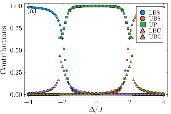
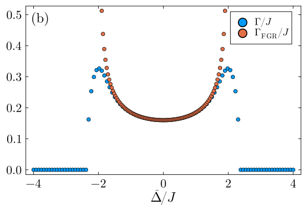
Figure 2: (a) Dynamical contributions to $W\left({t}\right)$, Eq. (33). There are three types of contributions to the contour integral. (i) Real poles: Lower (RL) and upper (UP). (ii) A single complex pole (CP) and (iii) branch cuts: Lower (LBC) and upper (UBC).(b) Comparison of the single emitter decay exact ($\Gamma$) and Markovian ($\Gamma_{\text{FGR}}=-\text{Im}\left({\Sigma_{1D}\left({\bar{\Delta}}\right)}\right)/2$) decay rates as a function of the detuning from the photonic crystal’s central frequency $\bar{\Delta}=\omega_{S}-\omega_{E}$. At the band edges the tight-binding model exhibits a diverging density of states, leading to non-Markovian behavior and a deviation between the Markovian and exact results. Model parameters: $g=0.4J$ ($g_{SE}=g$, $J=\Delta\omega_{E}$).

Comparing the two types of protocols, the non-Markovian contribution of the monochromatic pulse remains of similar magnitude throughout the dynamics, while for the Gaussian pulse the contribution exhibits a peak during the pulse and decays slowly in time. Surprisingly, for the pulse $f_{NM}$ obtains substantial values long after the pulse decays (see dashed-dotted yellow and dashed red line in panel (b)). Such behavior arises from the time non-local nature of the non-Markovian effects.

III.5 Two driven modes coupled to a 1D photonic crystal

The following section extends the single-mode analysis to a pair of nano-cavities, coupled to sites $\pm j_{S}$ of a 1D photonic crystal. The composite system is represented by the Hamiltonian

$$H=\omega_{S}\sum_{n=\pm{j_{{S}}}}a^{\dagger}_{n}a_{n}+g\sum_{n=\pm j_{S}}\left({a_{n}b^{\dagger}_{n}+a_{n}^{\dagger}b_{n}}\right)+H_{E}^{\left({t.b}\right)}\leavevmode\nobreak\ \leavevmode\nobreak\ .$$ (35)

Transitioning to the Fourier components decouples the environment’s collective modes and leads to an interaction term of the form $g\sum_{n=\pm j_{\text{S}}}\left({a_{n}b_{k}^{\dagger}e^{ikan}+a_{n}^{\dagger}b_{k}e^{-ikan}}\right)$.

Figure 3: Schematic representation of the studied linear model. Two driven modes situated at positions $\pm j_{S}$ with associated drives $f_{\pm j_{S}}\left({t}\right)$. The system modes are coupled locally, via a coupling strength $g$, to a 1D photonic crystal, represented by a chain of linear modes with nearest neighbour interactions of strength $J$. The tight-binding environment is characterized by rapidly varying density of states near the band edges, imposing strong non-Markovian system dynamics when $|\bar{\Delta}\pm J|\sim g$.

Reflection symmetry of the configuration enables decoupling the composite system into two collective system modes, $a_{\pm}$, which are coupled to two distinct environments González-Tudela and Cirac (2017). Thus, effectively reducing the analysis to a single mode problem. The system’s dynamics take the form

$$\bm{a}\left({t}\right)=\bm{W}\left({t}\right)\bm{a}\left({0}\right)+\bm{T}\left({t}\right)\bm{b}\left({0}\right)\leavevmode\nobreak\ \leavevmode\nobreak\ \\ -i\int_{0}^{t}\bm{W}\left({t-s}\right)\bm{f}\left({s}\right)ds\leavevmode\nobreak\ \leavevmode\nobreak\ ,$$ (36)

where

$$\bm{W}\left({t}\right)=\frac{1}{{2}}\left[{\begin{array}[]{cc}W_{+}+W_{-}&W_{+}-W_{-}\\ W_{+}-W_{-}&W_{+}+W_{-}\end{array}}\right]\leavevmode\nobreak\ \leavevmode\nobreak\ ,$$ (37)

and $W_{\pm}$ are the non-equilibrium Green function of the collective system modes $a_{\pm}=\left({a_{1}\pm a_{2}}\right)/\sqrt{2}$. These Green functions are given explicitly in Appendix C.2.

The non-diagonal form of $\bm{W}$ leads to a cross-coupling effect, where the drive on one of the system modes influences the other. The cross-coupling effect is demonstrated by considering a monochromatic drive only on the first system mode ($\bm{f}\left({t}\right)=\{A\exp\left({-i\omega_{L}t}\right),0\}^{T}$). The drive on the first mode leads to an additional non-Markovian term in the master equation, $f_{NM,2}\left({t}\right)$, driving the second mode. Here $f_{NM,i}$ denotes the $i$-th component of the vector $\bm{f}_{NM}$. The magnitude of non-Markovian cooperative effect increases with the system-environment coupling, Fig. 4. The distance between the system modes modifies the collective behaviour and thus, modifies the magnitude of $f_{NM,2}$ substantially. Figure 5 compares $f_{NM,2}$ for varying distances and emitters detuning $\bar{\Delta}$, for a Gaussian pulse applied to the first emitter. Well inside the band and in the band gap the magnitude of the non-Markovian cross effect decreases with the distance (Panels (a) and (d)). This is contrasted by the behavior close to the band edge, where the branchcuts’ contribution to the dynamics intensifies. For a plot of the various contributions to the contour integral of $W\left({t}\right)$ see González-Tudela and Cirac (2017) Fig. (4). For $\bar{\Delta}=-0.1J,-1J$ (Panels (b) and (c), respectively) $f_{NM,2}$ exhibits large magnitudes even for large emitter distances.

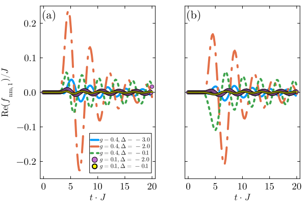
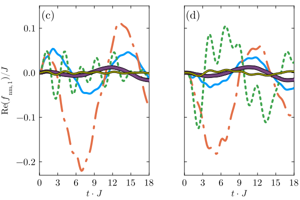
Figure 4: The non-Markovian drive term on the first $f_{NM,1}\left({t}\right)$ (a,c) and second mode $f_{NM,2}\left({t}\right)$ (b,d) as a function of time for different system-environment coupling and detunings. The first mode is driven by a Gaussian pulse in (a,b) and monochromatic laser in (c,d). The model parameters are identical to Fig. 1.

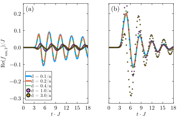
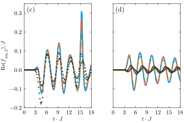
Figure 5: Effect of the distance $d$ between the system modes on $f_{NM,2}$, for varying detunings and a Gaussian laser pulse on the first system mode. Panels (a,b,c,d) correspond to the detunings $\\ bar{\Delta}=-3,-2,-1,-0.1$. $a=J=1$, $\delta=0.5J$, $\sigma_{L}=0.5J^{-1}$ and $A=2$, $g_{SL}=0.4J$.

III.6 Linear model validity regime

The presented analysis and results apply only to linear systems. Nevertheless, since in many cases the non-linearity of physical systems tends to be small Devoret et al. (1995), the analysis can either constitute a good approximation or serve as a basis for a perturbative treatment of the non-linearity. In addition, when the drive is sufficiently weak such that it generates simultaneously at most a single excitation shared among many particles, the Holstein-Primakoff approximation leads to an effective linear system. For instance, the presented analysis allows treating the dynamics of a weakly driven ensemble of Rubidium atoms in the Rydberg blockade regime Lukin (2003).

The analysis is not limited to the optical regime and applies to general driven linear systems coupled to a bosonic environment, where the composite dynamics are governed by a Hamiltonian of the form (3). For optical frequencies at room temperature, the electromagnetic state is well approximated by a vacuum state. However, when entering the IR regime and below temperature plays a significant role. The temperature effect can be incorporated into the construction following Ref. Yang et al. (2013). The presence of thermal excitations in the bath modifies the decay rates $\Gamma_{ij}^{\uparrow,\downarrow}$ and the coherent corrections $\Omega_{ij}$, see Appendix A.1. Notably, the Green function and the non-Markovian driving term $\bm{f}_{NM}\left({t}\right)$ is independent of the temperature.

IV Non-Linear optical systems

The dynamical behavior of driven linear and non-linear open systems is expected to be qualitatively different. For instance, the perturbative treatment of non-linear systems in the Markovian regime results in drive-dependent dissipative decay rates Kohler et al. (1997); Albash et al. (2012); Dann et al. (2018); Kuperman et al. (2020); Di Meglio et al. (2023); Mori (2023) and a drive-dependent memory kernel in a non-Markovian analysis Meier and Tannor (1999). Additionally, the linear case permits a normal mode analysis, while the combination of system non-linearities and the infinite degrees of freedom of the bosonic environment typically prevents exact solution. Specifically, the non-linearities imply that the composite Hamiltonian includes quadratic or higher-order terms. As a result, the operator algebra of the composite system (the primary system and environment) leads to an infinite hierarchy of coupled linear differential equations ( the Heisenberg equations) Bruus and Flensberg (2004). Despite of this fact, for a large class of non-linear systems, the driven open system dynamics can be connected to the dynamics of associated linear systems.

We show that the associated analytical linear solution can be harnessed to deduce a reliable dynamical solution for the corresponding non-linear system. The solution is manifested by a dynamical equation, termed the “Linear Master Equation” (LME). The LME is compared to a pseudo-mode solution, which simulates the effect of the environment on the primary system employing a small dissipative reservoir. In this case, the composite dynamics of the primary system and reservoir can be solved numerically to obtain an exact result. The comparison between the LME and pseudo-mode solution provides a way to analyze and interpret the interplay between the coherent and incoherent dynamical contributions, as well as the memory and cooperative effects of the drive.

We focus on the driven open system dynamics of an ensemble of two-level quantum emitters. The composite Hamiltonian is of the form

$$H\left({t}\right)=\sum_{ij}\sigma_{i}^{\dagger}M_{ij}\sigma_{j}+\sum_{i}\left({f_{i}\left({t}\right)\sigma_{i}^{\dagger}+f_{i}^{*}\left({t}\right)\sigma_{i}}\right)\\ +\sum_{ik}\left({g_{ik}\sigma_{i}^{\dagger}b_{k}+g_{ik}^{*}\sigma_{i}b_{k}^{\dagger}}\right)+\sum_{k}\omega_{k}b_{k}^{\dagger}b_{k}\leavevmode\nobreak\ \leavevmode\nobreak\ ,$$ (38)

where $\sigma_{i}=\left|g\right>_{i}\left<e\right|_{i}$ is the ladder operator of the $i$’th emitter and the environment is assumed to be initially in the vacuum state. Within the Markovian regime, dynamics of a variety of the optical, solid-state and molecular systems are well represented by Eq. (38) Barreiro et al. (2011); Wang et al. (2024); Doherty et al. (2013); Goldman et al. (2015); Pachón and Brumer (2011); Ishizaki and Fleming (2012); Blais et al. (2021). Beyond the Markovian regime, such an Hamiltonian may be realized by neutral and solid-state atoms interacting with photonic modes confined to engineered dielectric materials Lodahl et al. (2015); González-Tudela and Cirac (2017), cold atoms in a state-dependent optical lattice de Vega et al. (2008); Navarrete-Benlloch et al. (2011) and cavity QED setups Kimble (1998); Walther et al. (2006).

We begin by presenting the pseudo-mode technique Tamascelli et al. (2018); Garraway (1997a). In Sec. IV.2, we map the non-Markovian bosonic equation (4) to the LME, a master equation for the emitters, and benchmark its performance in the following sections. Physically, such a mapping involves neglecting the back reaction of the environment, associated with the system’s non-linearity. A priori, this approach is expected to provide a good description for a small number of excitations where the non-linearities are small. Nevertheless, we find an excellent agreement between the linear master equation and the pseudo-mode simulation even for moderate driving ($g_{SL}\sim\Gamma_{FGR}$), involving multiple excitations, and moderate system-environment coupling. The interplay between the coherent and incoherent dynamical contributions is studied in sections IV.3, IV.4, IV.6, while the drive dependent cooperative effects are investigated in Sec. IV.7.

Concluding the section, we focus on the standard optical regime in Sec. IV.6, involving moderate driving strengths and a Markovian environment. In this regime, the accuracy of the linear and optical Bloch master equations is compared to the Floquet Ho et al. (1986); Kohler et al. (1997); Breuer and Petruccione (1997); Chu and Telnov (2004); Szczygielski et al. (2013); Szczygielski (2014); Elouard et al. (2020), Adiabatic Albash et al. (2012) and Time-Dependent Di Meglio et al. (2023) master equations. The results of the final comparison highlights that within this regime, the influence of the drive on the dissipation can be neglected even for very intense lasers.

IV.1 Pseudo-mode solution

Simulation of the bosonic environment with dissipative pseudo-modes enables the evaluation of the exact driven open system dynamics. The simulation allows replacing an infinite number of modes with a finite number of so-called pseudo-modes, which are bosonic modes interacting with the system while simultaneously undergoing Markovian dissipation. Such an exact mapping is possible under the following conditions Tamascelli et al. (2018); Garraway (1997b): (a) The environment is bosonic, (b) it is initially in a Gaussian state, (c) the bare environment Hamiltonian is quadratic in the bosonic creation and annihilation operators, and (d) the spectral density of the environment can be well approximated in terms of a linear combination of Lorentzian functions.

Underlying the mapping are two key insights. First, the influence of the environment on the open system is completely determined by the system interaction operators in the interaction picture and the bare environment’s correlation functions . In addition, for a Gaussian initial state, Wick’s theorem implies that high-order correlation functions can be reduced to products of the first and second-order correlation functions. As a result, a bosonic field can be simulated by a reservoir including a finite number of modes, if the environment’s and reservoir’s first and second correlation functions, as well as the interaction operators in the interaction picture, coincide. Tamascelli et al. Tamascelli et al. (2018) provided a rigorous proof for the open system simulation of a bosonic Gaussian environment, focusing on a non-driven system. Nevertheless, as pointed out in Ref. Pleasance et al. (2020), the proof remains valid for any system Hamiltonian, including arbitrary time-dependent terms.

We consider identical coupling of the emitters to the environment, $g_{ik}=g_{k}$ (Eq. (38)), a Lorentzian spectral density function

$$J\left({\omega}\right)=\frac{1}{\pi}\frac{g_{SE}^{2}\kappa}{\left({\omega-\eta}\right)^{2}+\kappa^{2}}\leavevmode\nobreak\ \leavevmode\nobreak\ ,$$ (39)

and an environment initially in the vacuum state. The influence of the environment on the studied system can be precisely simulated by a reservoir, $R$, including a single dissipative pseudo-mode. The composite system-reservoir dynamics are given by

$$\frac{d}{dt}\rho_{SR}\left({t}\right)=-i\left[{H_{SR}\left({t}\right),\rho_{S}\left({t}\right)}\right]+2\kappa{\cal D}_{c,c^{\dagger}}\left[{\rho_{SR}\left({t}\right)}\right]\leavevmode\nobreak\ \leavevmode\nobreak\ ,$$ (40)

where $c$ is the annihilation operator of the pseudo-mode and the composite Hamiltonian reads

$$H_{SR}\left({t}\right)=H_{S}\left({t}\right)+\lambda\left({Sc^{\dagger}+S^{\dagger}r}\right)+\eta c^{\dagger}c\leavevmode\nobreak\ \leavevmode\nobreak\ ,$$ (41)

with $H_{S}\left({t}\right)=\sum_{ij}\sigma_{i}^{\dagger}M_{ij}\sigma_{j}+\sum_{i}\left({f_{i}\left({t}\right)\sigma_{i}^{\dagger}+f^{*}\left({t}\right)\sigma_{i}}\right)$ and $S=\sum_{i}\sigma_{i}$. The equivalence between the reduced dynamics, $\rho_{S}\left({t}\right)$, as obtained from the unitary description Eq. (38), and the dissipative system $\text{tr}_{R}\left({\rho_{SR}\left({t}\right)}\right)$ Eq. (40), is guaranteed by the equivalence of the interaction operators $S\left({t}\right)=U_{S}^{\dagger}\left({t}\right)SU_{S}\left({t}\right)$, where $U_{S}\left({t}\right)={\cal T}\exp\left({-i\int_{0}^{t}d\tau H_{S}\left({\tau}\right)}\right)$, and the second order correlation functions

$$C_{E}\left({t,0}\right)=\text{tr}_{E}\left[{\left({\sum_{k}g_{k}b_{k}e^{-i\omega_{k}t}}\right)\left({\sum_{k}g_{k}^{*}b_{k}^{\dagger}}\right)\rho_{E}\left({0}\right)}\right]\\ =\int_{0}^{\infty}J\left({\omega}\right)e^{-i\omega\tau}d\tau\approx{g_{SE}}^{2}e^{-\kappa\tau}\\ =\text{tr}_{R}\left({c\left({t}\right)c^{\dagger}\left({0}\right)\rho_{R}\left({0}\right)}\right)=C_{R}\left({t,0}\right)\leavevmode\nobreak\ \leavevmode\nobreak\ .$$ (42)

Here, both $\rho_{E}\left({0}\right)$ and $\rho_{R}\left({0}\right)$ are the respective vacuum states and the dynamics of $c\left({t}\right)=e^{-i\left({\eta-i\kappa/2}\right)t}c\left({0}\right)$ is evaluated with the adjoint master equation of Eq. (40). The approximation in the third line involves taking the bottom range of the integral to $-\infty$. This is well justified when the Lorentzian decays sufficiently fast $\kappa\ll\eta$. Physically, the approximation amounts to discarding the expected power-law decay at asymptotically large times Knight (1978).

To evaluate the system dynamics, the infinite states energy ladder of the pseudo-mode is truncated and the composite system-reservoir state is propagated with a standard numerical propagator. The number of Fock states required in the calculation can be estimated as $n_{\text{trunc}}>\left({g_{SE}g_{SL}}\right)/\left({\kappa\sqrt{g_{SE}^{2}+g_{SL}^{2}}}\right)$. The validity of the calculation was confirmed by comparing the solution to exact analytical results for non-driven systems Jaynes and Cummings (1963); Vacchini and Breuer (2010); Xia et al. (2024) and by verifying that the amplitude of the highest pseudo-mode eigenstates remains negligible throughout the evolution.

IV.2 Linear master equation

The bosonic master equation (4) provides a basis for an approximate equation of motion for the driven emitters’ open system dynamics. We assume the back-reaction of the environment is only negligibly affected by the non-linearity of the system, and map the bosonic operators to emitters’ ladder operators $b_{i}\rightarrow\sigma_{i}$

$$\dot{\rho}_{S}\left({t}\right)=-i\left[{\tilde{H}_{S}\left({t}\right),\rho_{S}\left({t}\right)}\right]\\ +\sum_{i,j=1}^{N_{S}}\Gamma_{ij}^{\downarrow}\left({t}\right){\cal D}_{\sigma_{j},\sigma_{i}^{\dagger}}\left[{\rho_{S}\left({t}\right)}\right]+\Gamma_{ij}^{\uparrow}\left({t}\right){\cal D}_{\sigma_{i}^{\dagger},\sigma_{j}}\left[{\rho_{S}\left({t}\right)}\right]\leavevmode\nobreak\ \leavevmode\nobreak\ ,$$ (43)

where ${\cal D}_{x,y}\left[{\bullet}\right]\equiv x\bullet y-\{yx,\bullet\}/2$, $N_{S}$ is the number of emitters

$$\tilde{H}_{S}\left({t}\right)=\sum_{i,j=1}^{N_{S}}\sigma^{\dagger}_{i}{\Omega}_{ij}\left({t}\right)\sigma_{j}+\sum_{i=1}^{N_{S}}\left({k_{i}\left({t}\right)\sigma_{i}^{\dagger}+k_{i}^{*}\left({t}\right)\sigma_{i}}\right)\leavevmode\nobreak\ \leavevmode\nobreak\ .$$ (44)

Here, the relaxation rates and coherent term are identical to those in the bosonic equation, given explicitly in Appendix A.1. Equation (43) defines the general form of the linear master equation (LME).

The conducted mapping can be understood in terms of the Holstein-Primakoff transformation Holstein and Primakoff (1940), which enables expressing spin operators in terms of bosonic operators. The substitution is the zeroth order of such a transformation and therefore is expected to be valid only in the low excitation regime Porras and Cirac (2008). Nevertheless, we find that Eq. (43) provides an accurate description of the reduced system dynamics beyond the low excitation regime. Finally, in the Markovian limit, the normalized frequencies and decay rates converge to the Markovian values described in Sec. (III), and the linear equation coincides with the well-known optical Bloch master equation Scully and Zubairy (1999).

IV.3 Single emitter Markovian regime

For a single driven emitter coupled to a bosonic environment, Eq. (38) simplifies to

$$H\left({t}\right)=\frac{\omega_{S}}{2}\sigma_{z}+f\left({t}\right)\sigma_{+}+f^{*}\left({t}\right)\sigma_{-}\\ +\sum_{k}\left({g_{k}\sigma_{+}b_{k}+g_{k}^{*}\sigma_{-}b_{k}^{\dagger}}\right)+\sum_{k}\omega_{k}b_{k}^{\dagger}b_{k}\leavevmode\nobreak\ \leavevmode\nobreak\ .$$ (45)

When the environment is initially in the vacuum state with a Lorentzian spectral density, Eq. (39), the emitter’s reduced dynamics can be simulated via an artificial environment consisting of a single ‘pseudo’-mode ($r$) undergoing dissipative dynamics Garraway (1997a); Tamascelli et al. (2018). The pseudo-mode’s Hilbert space is truncated, and the composite emitter-pseudo-mode density matrix dynamics are evaluated numerically.

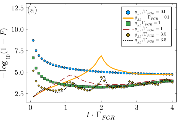
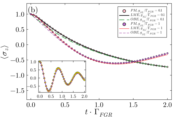
Figure 6: Monochromatic drive in the Markovian regime: Comparison of the LME (markers) and OBE (thin lines) for increasing driving strength. (a) Negative logarithm of the infidelity with respect to the pseudo-mode solution as a function of time. (b) Dynamics of $\langle{\sigma_{z}\left({t}\right)}\rangle$. Inset presents the PM (yellow circles), LME (continuous orange line) and OBE (dashed blue line) for $g_{SL}=3.6\Gamma_{FGR}$. The driving strength is large relative to the chosen detuning $\Delta=\omega_{S}-\omega_{L}=10^{-4}\omega_{S}$; for weaker driving the agreement between the LME and the PM solutions improves. Model parameters: $\left|\psi_{S}\left({0}\right)\right>=\left|e\right>$, $\Gamma_{FGR}=2\pi g_{SE}^{2}D\left({\omega_{S}}\right)\approx 0.011\omega_{S}\approx 0.055\Delta\omega_{E}$, $\Delta\omega_{E}=\kappa=0.2\omega_{S}$. The point at time $t=0$, where both solutions are exact, is excluded from all the infidelity comparisons.

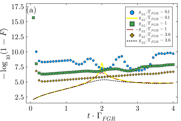
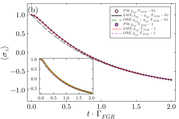
Figure 7: Gaussian pulse in the Markovian regime: Comparison of the performance of the LME (markers) and OBE (thin lines) for increasing driving strength. (a) Negative logarithm of the infidelity with respect to the pseudo-mode solution as a function of time. (b) $\sigma_{z}$ expectation value as a function of time. Inset: identical coloring as in Fig. 6, $g_{SL}=0.1\omega_{S}=3.6\Gamma_{FGR}$. Model parameters: $t_{0}=15/\omega_{S}=0.17\Gamma_{FGR}$, $\sigma_{L}\approx 2/\omega_{S}^{-1}=0.02\Gamma_{FGR}$, while the rest of the parameters are identical to Fig. 6.

We compare the pseudo-mode solution to the linear master equation (LME) (Eq. (43))

$$\dot{\rho}_{S}\left({t}\right)=-i\left[{H_{S}^{\left({LME}\right)}\left({t}\right),\rho_{S}\left({t}\right)}\right]+\Gamma^{\downarrow}\left({t}\right)D_{\sigma_{-},\sigma_{+}}\left[{\rho_{S}\left({t}\right)}\right]\leavevmode\nobreak\ \leavevmode\nobreak\ ,$$ (46)

with $H_{S}^{\left({LME}\right)}\left({t}\right)=\Omega\left({t}\right)\sigma_{+}\sigma_{-}+k\left({t}\right)\sigma_{+}+k^{*}\left({t}\right)\sigma_{-}$. For this simple model the normalized frequency and decay rates reduce to $\Gamma^{\downarrow}\left({t}\right)=-\left({A+A^{*}}\right)$, $\Omega\left({t}\right)=i\left({A-A^{*}}\right)/2$ with $A\left({t}\right)=\dot{W}/W$. The non-equilibrium Green function can be obtained from Eq. (6) by a Laplace transform

$$W\left({t}\right)=e^{-\left({i\omega_{S}-\kappa/2}\right)t}\left({\cosh\left({dt}\right)+\frac{\kappa}{2d}\sinh\left({dt}\right)}\right)\leavevmode\nobreak\ \leavevmode\nobreak\ ,$$ (47)

where $d=\sqrt{\left({\kappa/2}\right)^{2}-|\lambda|^{2}}$, for a Lorentzian spectral density, centered at $\eta=\omega_{S}$. In the Markovian limit, $\Gamma^{\downarrow}\left({t}\right)\rightarrow\Gamma_{FGR}=2\pi J\left({\omega_{S}}\right)$, $\Omega\rightarrow\omega_{S}$, $k\left({t}\right)\rightarrow f\left({t}\right)$, and the LME converges to the Optical Bloch Master Equation (OBE)

$${\cal L}^{\left({OBE}\right)}\left[{\bullet}\right]=-i\left[{{H}_{S}^{\left({OBE}\right)}\left({t}\right),\bullet}\right]+\Gamma_{FGR}{\cal D}_{\sigma_{-},\sigma_{+}}\left[{\bullet}\right]\leavevmode\nobreak\ \leavevmode\nobreak\ ,$$ (48)

with ${H}_{S}^{\left({OBE}\right)}\left({t}\right)=\left({\omega_{S}/2}\right)\sigma_{z}+g_{SL}\left({f\left({t}\right)\sigma_{+}+f^{*}\left({t}\right)\sigma_{-}}\right)$.

We start by analyzing the Markovian regime. Figure 6 benchmarks the LME and OBE master equations with respect to the PM solution, for increased driving strength. At short times ($t<1/\Gamma_{FGR}$) the LME closely matches the exact solution even for extremely strong driving, achieving fidelities as low as $F\approx 10^{-6}$ for $g_{SL}\sim 0.1\Gamma_{FGR}$. Increasing the driving strength leads to a decrease in accuracy (characterized by $-\log_{10}\left({1-F}\right)$) due to the non-linear effects, reaching infidelities of $1-F\sim 10^{-3}$. At intermediate times the accuracy of the OBE surpasses the LME while converging to similar accuracy at long times, Panel (a). Panel (b) showcases the typical dynamics of an emitter expectation value. Remarkably, the LME correctly captures the non-Markovian initialization step. Smoothly connecting the short-time quasi-unitary dynamics to the long-time exponential decay predicted by the OBE. For short times, the discrepancy between OBE and the exact result arises from finite information flow speed. Alternatively, the decay is quadratic in time $\langle{\sigma_{z}\left({t}\right)}\rangle\sim\exp\left({-\left({g_{SE}t}\right)^{2}}\right)$ as $t\rightarrow 0$ . The large deviation between the LME and OBE, e.g. Fig. 6 Panel (a) demonstrates that non-Markovianity may lead significant differences in accuracy, at times much larger than expected $\gg 1/\Delta\omega_{E}$ ($\sim 0.05/\Gamma_{FGR}$ in the in the model parameters of Fig. 6).

The Gaussian pulse exhibits an improved precision, as shown in Fig. 7. Before the pulse, the LME agrees with the PM to within numerical precision, while the OBE exhibits infidelities of the order $10^{-2}$. The pulse creates small deviations with respect to the exact result, obtaining an improvement of between one and two order of magnitude relative to the monochromatic laser. Such an improvement results from the restricted time-range of the drive. This reduces the population transfer between the ground and excited states and consequently the non-linear open system effects. The fidelity of the LME increases at long times, maintaining significant improvement in accuracy relative to the OBE prediction. This typical behavior differs qualitatively from the monochromatic laser case. Note that even for the strongest studied driving strength, the departure from the exact solution is unnoticeable in the emitter observable dynamics, e.g., inset of Panel (b).

IV.4 Narrow pulse bandwidth non-Markovian effect

For sufficiently short pulses, the laser bandwidth becomes comparable to the environment’s bandwidth. The competition between these timescales is expected to lead to novel dynamical effects Kruchinin (2019). This regime was explored by comparing the evolution of $\langle{\sigma_{z}\left({t}\right)}\rangle$ as predicted by the LME, OBE, and PM solutions for varying pulse standard deviation $\sigma_{L}$ of a normalized Gaussian pulse

Figure 8: Pseudo-mode, Linear and Optical Bloch master equation solutions for varying pulse width, $\sigma_{L}$. Panels (a) and (b) show the dynamics for fast (wide-bandwidth) and slow (narrow-bandwidth) pulses relative to the environment bandwidth ($\Delta\omega_{E}=0.2\omega_{S}$). Model parameters:Model parameters: $\Delta=10^{-5}\omega_{S}$, $\Gamma_{FGR}\approx 5\cdot 10^{-5}\Delta\omega_{E}$, $\Delta\omega_{E}=\kappa=0.2\omega_{S}$, $\eta=\omega_{S}$, $t_{0}=100/\omega_{S}$ and an initial composite state $\left|\psi\left({0}\right)\right>=\left[{\left({\left|g\right>+\left|e\right>}\right)/{\sqrt{2}}}\right]\otimes\left|\text{vac}\right>$.

The qualitative behavior depends on the ratio between the pulse and environment bandwidths ($\Delta\omega_{E}=\kappa=0.2\omega_{S}$). For an ultra-short pulse ($\sigma_{L}^{-1}=50\kappa$, Fig. 8, Panel (a)) the pulse is much faster than the fastest timescale of the composite system in the rotating frame ($\kappa$). As a result, the sudden approximation holds, and the system and environment cannot respond to the rapid Hamiltonian change Sakurai and Napolitano (2020) . When the pulse’s bandwidth is narrower, yet within the environment’s range ($\sigma_{L}^{-1}=5\kappa$, green circles), the pulse causes a rapid shift in the expectation value, which is not captured by both the LME and OBE solutions. Decreasing the pulse’s bandwidth below the environment’s smooths out the rapid shift (Panel (b), pink circles). This behavior is only partially captured by the LME and OBE (orange and black continuous lines, respectively), which overestimate the feature. For slower pulses relative to $\Delta\omega_{E}$ (narrow bandwidth), the shift in $\langle{\sigma_{z}}\rangle$ is smoothed out further (cyan circles), which is accurately predicted by both the LME and OBE solutions.

To conclude, for sufficiently rapid driving (in the rotating frame), where the pulse and environment bandwidths become comparable, non-Markovian effects may give rise to deviations between the LME (OBE) and the exact solution. In the ongoing efforts to achieve faster control protocols and combat inevitable dissipation processes, it is expected that even in experiments done in free space precise control will soon require accounting for such non-Markovian effects. Alternatively, in highly non-Markovian environments, such as high-Q cavity QED, even narrow-band pulses can match the cavity decay rate $1/\tau_{\text{decay}}\sim\Delta\omega_{E}$. In this regime, narrow-bandwidth non-Markovian effects could be demonstrated in tabletop cavity QED experiments

IV.5 Non Markovian regime

When the linewidth ($\Gamma_{FGR}$) becomes comparable to the environment bandwidth, the non-Markovian become significant. The LME then provides an accurate solution of the dynamics for the short and intermediate time regimes and moderate driving strength, Fig. 9 Panel (a). For a monochromatic drive, the accuracy of the LME drops sharply due to the non-linear corrections, while for a Gaussian pulse, the solution remains accurate even at long times, Panel (b). Panel (c) compares the non-Markovian (LME) and Markovian (OBE) evolution of $\langle{\sigma_{z}\left({t}\right)}\rangle$. As depicted in the figure, the non-Markovianity modifies the solution substantially.

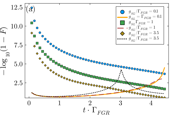
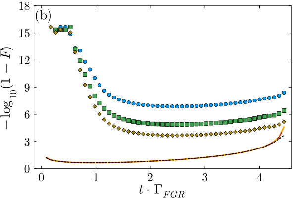
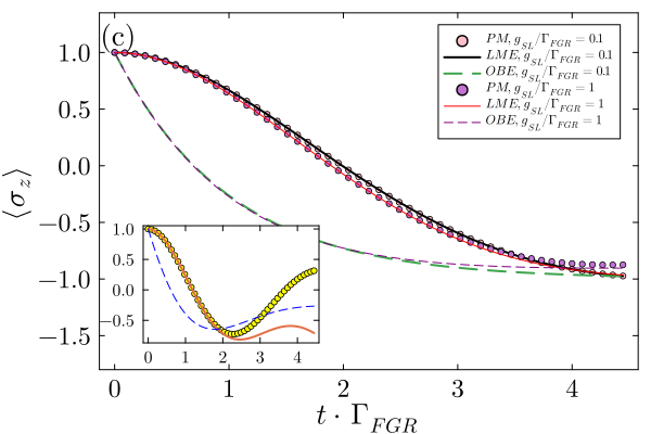
Figure 9: Non-markovian dynamics: Infidelity (a,b) and $\langle{\sigma_{z}\left({t}\right)}\rangle$ as a function of time for a monochromatic laser (a,c) and Gaussian pulse (b). Model parameters: $\Gamma_{FGR}/\Delta\omega_{E}=0.4$, $\Delta\omega_{E}=0.03\omega_{S}$ and $\left|\psi_{S}\left({0}\right)\right>=\left|e\right>$. The Gaussian pulse is centered at $t_{0}\approx 1.1/\Gamma_{FGR}$ with a root mean square of $\sigma_{L}\approx 0.15\Gamma_{FGR}$.

IV.6 Drive dependent dissipation: comparison to the Adiabatic, Floquet and Time-dependent master equations

A central question in the study of driven open systems is: Does the coherent drive affect the dissipation rates? To address this issue, we benchmark the performance of the Adiabatic (AME) Albash et al. (2012), Floquet (FME) and Time-Dependent (TDME) Di Meglio et al. (2023) master equations, which incorporate the influence of the drive on the dissipation rates.

The derivations of the LME and OBE master equations are directly connected to the primary system’s Heisenberg equations of motion Scully and Zubairy (1999), predict independent decay rates. An alternative approach considers a time-dependent Hamiltonian representing the driven system’s interaction with its environment. Starting with the complete dynamical description governed by the Liouville von-Neumann equation and relying on weak system-environment coupling and Markovianity, a series of approximations leads to the reduced system dynamics of the driven system Albash et al. (2012); Ho et al. (1986); Kohler et al. (1997); Breuer and Petruccione (1997); Chu and Telnov (2004); Yamaguchi et al. (2017); Szczygielski et al. (2013); Szczygielski (2014); Dann et al. (2018); Mozgunov and Lidar (2020); Elouard et al. (2020); Di Meglio et al. (2023). Alternatively, this approach can also be motivated by an axiomatic method employing dynamical symmetries Dann and Kosloff (2021); Dann et al. (2022).

Several constructions have been introduced, typically focusing on specific driving regimes and following the Born-Markov-secular approximations Breuer and Petruccione (2002) or employ projection operator techniques Nakajima (1958); Zwanzig (1960). For slow driving, the approach leads to an adiabatic master equation Albash et al. (2012), where the reduced dynamics follows the instantaneous composite Hamiltonian. The physical interpretation, in this case, involves environment induced transitions in an instantaneous eigenbasis of the primary system and drive combined Hamiltonian. For rapid oscillatory driving, the Floquet theorem leads to the Floquet master equation Ho et al. (1986); Kohler et al. (1997); Breuer and Petruccione (1997); Chu and Telnov (2004); Szczygielski et al. (2013); Szczygielski (2014). The derivation of the FME uses a Fourier decomposition of the system interaction operators in the interaction picture. Such decomposition enables applying the Born-Markov-Secular approximation scheme, leading to a Lindblad form with drive dependent kinetic coefficients Elouard et al. (2020). Here, the dissipation is captured by transitions between the Floquet states, which for a monochromatic drive correspond to the so-called dressed states Cohen-Tannoudji et al. (1998).

Recently, generalizations for non-periodic and non-adiabatic drives have been proposed Yamaguchi et al. (2017); Dann et al. (2018); Mozgunov and Lidar (2020); Di Meglio et al. (2023). Notability, Ref. Di Meglio et al. (2023) combines the projection operators technique with a rescaling of time, in the spirit of the seminal work of Davies Davies (1974). This procedure leads to what we refer to as the Time-Dependent master equation. In the interaction picture, relative to the primary system dynamics and drive, the TDME is characterized by adiabatic Lindblad jump operators and kinetic coefficients. The non-adiabaticity in this approach arises when transforming back to the Schrödinger picture, performed using the numerically evaluated exact time-evolution operator for the isolated system.

The different master equations may generally differ in both their operator structure and kinetic coefficients. As a result, they commonly provide distinct physical predictions, even within the same driving regime. This diversity stems from the variety of possible technical ways the basic physical approximations can be conducted. Moreover, change of the order of approximations may also modify the final result. An axiomatic approach has been developed to resolve this apparent ambiguity Dann and Kosloff (2021); Dann et al. (2022). Within this framework, a number of axioms are postulated and utilized to prove the structure of the corresponding master equation. However, the construction is based on strong dynamical symmetries of the composite Hamiltonian, which in practice may not necessarily hold.

In the interaction picture relative to the central laser frequency, $\omega_{L}$, the AME, FME and TDME are of the form

$${\cal L}_{\text{A}}=-i\left[{\tilde{H}_{S}\left({t}\right),\bullet}\right]+{\cal D}^{\left({\text{A}}\right)}\left[{\bullet}\right]\leavevmode\nobreak\ \leavevmode\nobreak\ ,$$ (49)

with distinct dissipators $\text{A}=\text{AME, FME, TDME,}$ given explicitly in Appendix D. Notably, in order to accurately evaluate the Markovian decay rates of ${\cal D}^{\left({A}\right)}$ one must account for the shift in the environment’s spectrum and density of states, due to the transition to the rotating frame. In the rotating frame, the spectrum range is given by $\Delta_{k}\in[-\omega_{L},\infty)$, and the spectral density function becomes $\tilde{J}\left({\omega}\right)=\left({g_{SL}^{2}\kappa/\pi}\right)/\left[{\left({\omega-\left({\eta-\omega_{L}}\right)}\right)^{2}+\kappa^{2}}\right]$.

For a monochromatic drive since we are working in a rotated frame $\tilde{H}_{S}$ is independent of time, therefore the adiabatic theorem is exact. In addition, in such a frame the TDME coincides with the AME. Meaning that both master equations represent the dissipation in terms of transitions between the system’s dressed states. Such a description leads to Lindblad jump operators which depend on the control parameters.

Here we summarize the main findings, while the corresponding Figure (F) is presented in Appendix F. In the weak driving regime, $\Delta\gg g_{SL}$, the FME and AME converge to the OBE, where $\Delta=\omega_{S}-\omega_{L}$ is the detuning with respect to the central laser frequency. In contrast, for comparable $\Delta\sim g_{SL}$ or small $\Delta\ll g_{SL}$ detuning, the FME and AME deviate from the exact result. For a monochromatic drive (Gaussian pulse) the FME, AME and TDME achieve an accuracy in the range $-\log\left({1-F}\right)=0.1-2$ (0.1-4) while the LME and OBE showcase a substantially improved infidelities $F=10^{-3}-10^{-6}$ ($10^{-3}-10^{-10}$), for varying driving strengths.

Overall, the results highlight that within the studied parameter regime, the interpretation that the environment induced transitions between the Floquet or dressed states leads to the wrong dissipative decay rates.

IV.7 Two emitters Markovian and non-Markovian regimes

The coupling of multiple emitters to common environmental modes enables analyzing the influence of the non-linearities and memory effects on the collective behavior. The LME exhibits a good agreement with the exact solution for both short and long times in the Markovian regime, and up to intermediate times in the non-Markovian regime. The relative accuracy enables understanding and interpreting the driven open system dynamics by means of the different terms of the master equation.

The form of the LME is given in Eq. (43), with its coefficients determined by the non-equilibrium Green “function” $\bm{W}\left({t}\right)$. For the studied model, $\bm{W}\left({t}\right)$ can be calculated employing the Heisenberg equations of motion of the pseudo-mode solution. For two emitters with an identical detuning $\Delta$, an explicit analytical form for the Green function is readily obtained. It corresponds to the upper left two-by-two matrix $\exp\left({-i{\cal M}t}\right)$, where $\cal{M}$ is defined by the Heisenberg equation of motion $\dot{\bm{v}}=-i{\cal M}{\bm{v}}$, with ${\bm{v}}=\{a_{1},a_{2},r\}^{T}$, see Appendix E for further details.

In the Markovian limit, the LME converges to the OBE, which reads (in the rotated frame)

$$\frac{d}{dt}\rho_{S}\left({t}\right)=-i\left[{H_{S}\left({t}\right)+\sum_{n,m=1,2}J_{nm}^{\left({OBE}\right)}\sigma_{m}^{\dagger}\sigma_{n}}\right]\\ +\sum_{nm}\Gamma_{nm}^{\left({OBE}\right)}{\cal D}_{\sigma_{m}^{\dagger},\sigma_{n}}\left[{\rho_{S}\left({t}\right)}\right]\leavevmode\nobreak\ \leavevmode\nobreak\ .$$ (50)

For a Lorentzian spectral density and identical emitter coupling ($g_{ik}=g_{k}$), the shifts are $J_{nm}^{\left({OBE}\right)}=-\frac{|\lambda|^{2}\bar{\Delta}}{{\tilde{\Delta}}^{2}+\kappa^{2}}$, and the decay rates read $\Gamma_{nm}^{\left({OBE}\right)}=\frac{2|\lambda|^{2}\kappa}{{\tilde{\Delta}}^{2}+\kappa^{2}}$, where $\tilde{\Delta}=\eta-\omega_{L}$.

The comparison between the LME and OBE shows similar qualitative behavior to that observed in the single emitter case. As depicted in Fig. 10 Panel (a), for a monochromatic drive and moderate driving strength $g_{SL}/\Gamma_{FGR}\lesssim 1$, the LME exhibits exceptionally good infidelity at short times ($t\leq 1/\Gamma_{FGR}$), which increases to $1-F\sim 10^{-3.5}$ until $t\sim 2/\Gamma_{FGR}$ and to $1-F\sim 10^{-2.7}$ for longer times. In the strong driving regime ($g_{SL}/\Gamma_{FGR}=3.6$) the intermediate time infidelity remains above $10^{-2.5}$, and increases to above $10^{-2}$ at long times. At intermediate and long times the OBE outperforms the LME, achieving an improvement of around an order of magnitude in the infidelity. Contrastly, for a Gaussian pulse, the LME remains accurate even for very strong driving, Fig. 10 Panel (b).

Figure 10 Panel (b) presents the infidelity for weakly driven and non-driven initially two excited emitters. In contrast to the single emitter case, when the initial state includes multiple excitations, even in the absence of coherent driving the LME deviates from the exact result. Hence the obtained infidelity $<10^{-3.3}$ throughout the whole studied time duration ($t\leq 4/\Gamma_{FGR}$) constitutes a surprisingly good agreement with the exact result.

In the non-Markovian regime ($\Gamma_{FGR}/\kappa\approx 0.6$, $g_{SE}/\kappa=0.55$), the LME accurately captures the dynamics until $t\approx 1/\Gamma_{FGR}$, where the infidelity increases above $10^{-2.5}$, see Fig. F Appendix F. At longer times the prediction of the OBE surpasses the LME ($t>3/\Gamma_{FGR}$), which leads to the conclusion that a combination of the LME at short times and OBE at longer times may reliably capture the emitter dynamic beyond the Markovian regime.

Overall, the analysis of a single and two emitters evolution motivates the following interpretation of the dynamics. At short times ($t<1/\left({2\Gamma_{FGR}}\right)$), the non-linear effects remain small due to a minuscule two photons emission amplitude. It is enhanced once there is a substantial probability for the emitters to emit and reabsorb multiple photons ($t\sim 1/\Gamma_{FGR}$). This process leads to a rapid increase in infidelity, which reaches a maximum at $\sim t=1/\Gamma_{FGR}$. At longer times the inherent memory loss of the environment suppresses the probability to reabsorb a photon, and the infidelity of the LME improves up to $10^{-4}$, for the studied time-duration ($t\leq 4/\Gamma_{FGR}$). The typical trend of the accuracy for a weakly driven single emitter, as well as the non-driven multiple emitters, suggests that the major source of inaccuracies of the LME is the incomplete characterization of the reabsorption process.

IV.8 Substantial short-time non-Markovian corrections

The excellent agreement of the LME with the exact result at short times ($t<1/2\Gamma_{FGR}$), and the large deviation from the OBE solution (Figs. 6, 9, 10) implies that even in the Markovian regime, for times $t<1/(2\Gamma_{FGR})$, the dynamics can be significantly influenced by the non-Markovian corrections. These non-Markovian effects manifest at times much longer than expected. In the studied Markovian models, the environment bandwidth is chosen as $\kappa=0.2\omega_{S}\approx 18\Gamma_{FGR}$, hence one would expect that non-Markovian corrections occur at times comparable to $t\sim 1/\kappa\sim 0.06\Gamma_{FGR}$. Surprisingly, the results for single and two emitters suggest a contribution which influences the dynamics at much longer times.

Remarkably, the presented results suggest that the non-Markovian linear coefficients $\bm{f}_{NM}\left({t}\right)$, ${\Gamma}^{\downarrow}_{ij}\left({t}\right)$ (Eqs. (8) and (4)) accurately capture the dynamics of weakly driven dissipative emitters and the short-time dynamics of strongly driven emitters.

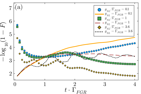
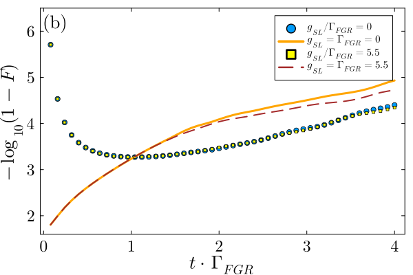
Figure 10: Two emitter Markovian dynamics: (a) Monochromatic drive (b) Gaussian pulse and a non-driven system. Model parameters: $\left|\psi_{S}\left({0}\right)\right>=\left|e\right>_{1}\otimes\left|e\right>_{2}$, $\Delta=10^{-4}\omega_{S}$, $\Delta\omega_{E}=\kappa=0.2\omega_{S}$, $\Gamma_{FGR}=2\pi g_{SE}^{2}D\left({\omega_{S}}\right)=9\cdot 10^{-2}\kappa$.

V Experimental realization

The major experimental challenge in the study of driven open system dynamics is the requirement for precise characterization, understanding and possible control of the environment. Namely, the environment in the experiment should precisely correspond to the theoretical model. This requires sufficiently slow dephasing of the environment and system due to unaccounted or uncharacterized noise. In practice, in order to observe most of the analysed phenomena it is sufficient to limit the dynamics to times up to $\sim 3/\Gamma_{FGR}$. Therefore, experimental platforms enabling loss rates of $\gamma\sim 0.1\Gamma_{FGR}$ are well suited for the task. An additional desirable property is the ability to tune the system-environment coupling to the range of the environment’s bandwidth $g_{SE}\sim\Delta\omega_{E}$, and maintain large Rabi-frequencies $g_{SL}\sim\Gamma_{FGR}$, while keeping the loss rates low. Several platforms meet these requirements, enabling the simulation of the environmental effect in a controllable manor and allowing for high-accuracy investigation of the non-Markovian effects. The leading platforms are (i) Engineered dielectric materials Lopez (2003); Lodahl et al. (2015), (ii) cold atoms in state dependent optical lattices de Vega et al. (2008); Navarrete-Benlloch et al. (2011) and (iii) cavity QED Kimble (1998); Walther et al. (2006).

Patterning the structure of dielectric material enable control of the refractive index and engineering the dispersion relation of the confined photonic modes Lopez (2003); Lodahl et al. (2015). In this platform, a single system harmonic mode can be realized by introducing a point defect within a periodic dielectric material. The defect creates an effective highly tubable nano-cavity for the propagating light modes in the material. Alternatively, a 1D (and 2D) tight-binding model environment, studied in Sec. III.4, can be realized by a series of defects forming a coupled resonator optical waveguide Yariv et al. (1999). Couplings and system environment parameters are readily tuned by modifying the refractive index of the photonic crystal by mechanical meansPark and Lee (2004), thermooptic Wang et al. (2011) and electrooptical Du et al. (2004) effects.

Non-linear open systems can be readily realized by coupling solid-state, quantum dots, or natural atoms to a photonic crystal Hung et al. (2013); Goban et al. (2014); Lodahl et al. (2015). A suitably designed refractive index then enables mimicking the environment’s spectral density function. Notably, to simulate the environment’s influence, it is sufficient to reproduce its spectral density or density of states within a limited frequency range on the order of the emitter linewidth, ${\sim\left[{\omega_{S}-n\Gamma_{FGR},\omega_{S}+n\Gamma_{FGR}}\right]}$, where $n$ is a small integer. Cohen-Tannoudji et al. (1998). This simplification allows the large tunability of the spectral properties of photonic crystals to be used to simulate the effects of band-less environments. Finally, for a 1D and 2D models the drive is realized by applying external lasers perpendicular to the photonic crystal’s surface Lei and Zhang (2012); Englund et al. (2009).

Coupling strengths of order $g_{SE}\sim 10$ GHz, and a bandwidth of $J=\Delta\omega_{E}\sim 5$ THz in the optical regime has been achieved Douglas et al. (2015). As expected, inside the band the emitter decay is indeed Markovian ($g_{SE}/\Delta\omega_{E}\sim 10^{-3}$), nevertheless, non-Markovian dynamics emerge near the band edge (1D) or van Hove points (2D and 3D), where the group velocity vanishes and the density of states diverges González-Tudela and Cirac (2017, 2018). Rabi-frequency of the order of $g_{SL}\sim\Gamma_{FGR}$ have been obtained, allowing to saturate the transition Zrenner et al. (2002). The primary source of decoherence is the emission to free space, which can be low as $\gamma\sim 5$ MHz Douglas et al. (2015), reaching the desired dynamical regime $\Gamma_{FGR}\gg\gamma$ with $g_{SE}\sim\Delta\omega_{E}$.

In the cold atom realization, two metastable states of a natural atom interact with different optical lattice potentials. A thorough analysis provided in Refs. de Vega et al. (2008); Navarrete-Benlloch et al. (2011); González-Tudela and Cirac (2017), here we summarize the main features of the proposal. The primary system is realized by an atomic state which interacts with a strong laser, manifesting a deep lattice potential. This results in localized Wiener states at each potential well and inhibits tunneling to near by sites. The bosonic environment is realized by a second state, interacting with a shallow lattice potential which enables transition between neighboring sites. Importantly, the atomic density and magnetic fields are tailored to suppress any interaction between the atoms. Moreover, the atomic motion is confined to the lowest Bloch band in the collisional blockade regime, where at most a single atom occupies a potential site. The system environment coupling is controlled by laser driven direct optical or two-photon Raman transitions. Coupling strengths of the order of the tunneling rates can be achieved $g_{SE}\sim J=\Delta\omega_{E}\sim 10$ KHz, while the strong driving regime can be reached using Rydberg atoms, manifesting Rabi-frequencies of the order of $g_{SL}\sim 10$ MHz Bloch et al. (2008).

The dominant sources of noise are scattering events induced by the trapping lasers and residual relaxation during the Raman transitions. These can be reduced to as low as $\gamma\sim 1$ Hz Bloch et al. (2008); Schreiber et al. (2015); Daley et al. (2008), reaching the desirable decoherence regime $\gamma/\Gamma_{FGR}\sim 10^{-3}$.

The well established field of cavity QED can also be employed to analyze the non-Markovian effects of the drive within the rotating wave approximation Kimble (1998); Haroche and Raimond (2006); Walther et al. (2006). Specifically, the mapping between the reduced dynamics of bosonic environments, initially in a Gaussian state, and the dynamics of a system coupled to dissipative pseudo-modes Tamascelli et al. (2018); Garraway (1997b) (Sec. IV.1) enables straightforward simulation of the driven open system dynamics, employing atoms or ions coupled to leaky cavities. The simplest case of emitters interacting with a Lorentzian spectral density environment, studied in Sec. IV, is realized by the standard QED setup, involving trapped emitters within a dissipative cavity. Coherent control is realized by directing lasers at the emitters. The strong coupling regime, $g_{SE}\sim\kappa=\Delta\omega_{E}$, is achieved by using Rydberg atoms, confined in a high finesse cavity or near a whispering-gallery mode cavity, while suppressing the emission to other electromagnetic modes ($\kappa$ is the cavity linewidth).

State-of-the-art optical cavities as the Fabry-Pérot (whispering-gallery mode cavities) achieve linewidths of $\kappa\sim 1-10$ kHz Della Valle et al. (2014) ($100\text{ kHz}–1$ MHz) with optimal coupling $g_{SE}\sim 100$ MHz ($\sim$ GHz), Rabi frequencies up to $g_{SL}\sim 10$ MHz for Rydberg atoms and free-space emission as low as $\gamma\sim 3$ MHz ($10$ MHz) Kimble (1998); Buck and Kimble (2003); Foreman et al. (2015). For modest values of $g_{SE}=10\kappa=100$ MHz, one obtains $\gamma/\Gamma_{FGR}\sim 10^{-2}$, which allows capturing the non-Markovian effects of the drive.

Finally, circuit QED experimental setups permit probing the non-Markovian effects of the drive and the interplay between coherent driving and dissipation beyond the rotating wave approximation Blais et al. (2021). Namely, the so-called ultra-strong coupling regime can be achieved, where the coupling is engineered to be larger than the system frequencies Bourassa et al. (2012) ($g_{SE}/\kappa\sim 10^{2}-10^{4}$ with $\kappa$ as low as $\sim 10$ kHz and decay rates of order $\gamma\sim$kHz, and Rabi-frequencies up to $g_{SL}\sim$ MHz Blais et al. (2021)). Here, non-Markovian dynamics are realized by coupling a superconducting LC resonators (linear system) or superconducting qubits (non-linear system) to planar superconducting resonators, such as coplanar waveguides or 3D microwave cavities (the environment). An external drive can be readily applied using microwave currents.

VI Conclusions and perspective

The interplay between coherent driving, dissipation and environmental memory effects generates a rich spectrum of dynamical phenomena. This study aimed to shed light on the mechanisms that govern the evolution of driven open quantum systems by comparing the performance of Markovian and non-Markovian master equations. Grasping the intricate interplay is vital not only for analyzing laser-induced phenomena in natural systems Blankenship et al. (2011); Huelga and Plenio (2013); Hubbard (1964); Holstein and Primakoff (1940), but also for advancing technological applications Verstraete et al. (2009). The ability to accurately capture these dynamics using simplified yet precise equations of motion offer promising avenues for the precise control and manipulation of open quantum systems Koch (2016); Dann et al. (2018); Kallush et al. (2022).

Starting with a linear composite system, the exact drive-dependent non-Markovian effects were examined. Using the resolvant formalism, these corrections were directly linked to the spectral features of the environment. Notably, this effect is independent of the environment’s temperature and arises from the initial state of the electromagnetic field (including the laser modes). This constitutes a distinct source of non-Markovianity, typically related to the spectral features of the environment.

Collective non-Markovian effects were subsequently studied, highlighting a novel cross-driving effect. Following, the general form of the exact master equation for a linear primary system, beyond the rotating wave approximation, was analyzed in Sec. III.2. The deduced master equation highlights that for arbitrary quadratic composite Hamiltonians and an initial Gaussian field state, the dissipation is independent of the drive.

An extension of the non-linear master equation, the linear master equation, was introduced (Sec. IV.2) and compared to an exact pseudo-mode solution. The comparison yields several key conclusions:

1. For an ensemble of emitters, non-Markovianity leads to modified time-dependence of the decay rates, bare system Hamiltonian, and external driving terms, which can be understood through a well-established analytical treatment of a corresponding linear system.

2. The non-Markovian corrections can manifest as cooperative dissipative and driving terms, as well as coherent interactions, in both linear and non-linear open systems.

3. The excellent accuracy of the driven single and two-emitter open system dynamics, for moderate drives and non-Markovianity, suggests that the back-action of the environment on the system is only slightly affected by the non-linearity.

4. Open system dynamics involving memory effects may be significantly affected by drive-dependent non-Markovian effects. This is manifested by a large magnitude of $\bm{f}_{NM}$ (Sec. III, Figs. 1 and 4).

5. In the analyzed non-linear systems, the dissipative decay rates are only negligibly affected by the drive.

6. Even within the Markovian parameter regime, when the bandwidths of the laser pulse and environment are comparable, non-Markovian effects lead to observable phase shifts (Sec. IV.4).

7. Non-Markovian effects can influence the relative accuracy of the evolution for times well beyond the typical decay time of environmental correlations.

8. For multiple non-driven emitters, the excellent accuracy of the LME provides a way to analytically investigate the multi-excitation regime.

The exceptional accuracy of the LME, at short times and within the Markovian regime (sections IV.3 and IV.7), is especially relevant for information processing tasks including quantum error correction. A typical quantum information procedure involves applying control fields to a quantum device (the primary system), weakly coupled to its surrounding environment, between repeated measurements Nielsen and Chuang (2010). To suppress errors, the measurements must be performed at time intervals which are small relative to the typical decoherence time ($\tau_{\text{meas}}<1/\Gamma_{FGR}$). Crucially, after each set of measurements, the composite system-environment state collapses to a product state, before the inevitable emergence of new system-environment correlations. In this context, the analyzed short-time dynamics may correspond to the evolution between two subsequent measurements of a realistic quantum device. As a result, the accurate short-time description of the LME can be harnessed to engineer improved quantum gates, which account for the environmental noise Kallush et al. (2022).

To illuminate the nature of interference between coherent driving and dissipation, we compared in Sec. IV.6 the performance of the Floquet, Adiabatic, and Time-Dependent master equations with the LME and its Markovian limit, the optical Bloch master equation. We found that the Markovian master equations incorporating the drive into the dissipation process (FME, AME, and TDME) deviate substantially from the exact solution. This comparison supports the conclusion that even for relatively strong driving, within the standard quantum optics regime, the dissipation remains independent of the drive.

The experimental considerations involved in realizing the drive-related open system phenomena were detailed in Sec. V. Analog simulation of open system dynamics proves to be a challenging task due to the inevitable interaction of the environment and primary system with uncontrolled sources of noise. Nevertheless, a number of state-of-the-art devices enable experimental confirmation of the proposed dynamical effects.

An extension of the present analysis to finite-temperature thermal environments can be is achieved by using the general relation of the non-Markovian kinetic coefficients in Appendix A.1. The present analysis is however limited by the implicit application of the rotating wave approximation, leading to the considered Hamiltonian form. The analysis is therefore valid under the condition $g_{SL}\ll\omega_{S}$ .

Finally, there are several possible extensions of the present analysis that are of significant interest. Future work may focus on including higher-order corrections of the non-linearity to the linear master equation and generalization to multi-level (beyond two-level) systems. Alternatively, the interplay between the counter rotating terms and coherent driving should be investigated Cao et al. (2021). Furthermore, the linear master equation can be applied to characterize the non-Markovian influence of environmental spectral features and laser pulses on collective phenomena such as superradiance Dicke (1954); Gross and Haroche (1982) and subradiance Guerin et al. (2016), the quantum state of emitted light Parkins et al. (1995); Matsukevich and Kuzmich (2004); Porras and Cirac (2008); Mitsch et al. (2014); Pizzi et al. (2023); Tziperman et al. (2024), and dispersive interactions between quantum emitters Buhmann (2013); González-Tudela and Cirac (2017).

Appendix A Non-Markovian master equation of linear systems

A.1 Non Markovian kinetic coefficients

Considering a bosonic composite system, including a set of system modes coupled to a bosonic environment, initially in a thermal state with inverse temperature $\beta$. The decay rates and coherent parameters are the elements of the following matrices

$$\bm{\Gamma}^{\downarrow}\left({t}\right)=\dot{\bm{V}}-\dot{\bm{W}}\bm{W}^{-1}\left({\bm{V}+\bm{I}}\right)-\left({\bm{V}+\bm{I}}\right)\left({\dot{\bm{W}}\bm{W}^{-1}}\right)^{\dagger}$$ (51)

$$\bm{\Gamma}^{\uparrow}\left({t}\right)=\dot{\bm{V}}-\dot{\bm{W}}\bm{W}^{-1}\bm{V}-\bm{V}\left({\dot{{\bm{W}}}\bm{W}^{-1}}\right)^{\dagger}$$

$$\bm{\Omega}\left({t}\right)=\frac{i}{2}\left[{\dot{\bm{W}}\bm{W}^{-1}-\left({\dot{\bm{W}}\bm{W}^{-1}}\right)^{\dagger}}\right]\leavevmode\nobreak\ \leavevmode\nobreak\ ,$$

with

$$\bm{V}\left({t}\right)=\bm{T}\left({t}\right)\bm{n}_{BE}\left({\bm{E}}\right)\bm{T}^{\dagger}\left({t}\right)\leavevmode\nobreak\ \leavevmode\nobreak\$$ (52)

$$\bm{T}\left({t}\right)=-i\int_{0}^{t}d\tau\bm{W}\left({t-\tau}\right)\bm{R}e^{-i\bm{E}\tau}\leavevmode\nobreak\ \leavevmode\nobreak\ ,$$ (53)

where $\bm{n}_{BE}=1/\left({\exp\left({\beta\bm{E}}\right)-1}\right)$, ($\bm{E}=\text{diag}\left({\omega_{1},\dots,\omega_{N_{E}}}\right)$) is a diagonal matrix including the thermal populations, given by the Bose-Einstein distribution and $\bm{R}$ is the coupling matrix, determined by Eq. (16).

For a fermionic composite system the $\bm{\Gamma}^{\downarrow}$ is slightly modified

$$\bm{\Gamma}^{\downarrow}\left({t}\right)=-\dot{\bm{V}}+\dot{\bm{W}}\bm{W}^{-1}\left({\bm{V}-\bm{I}}\right)+\left({\bm{V}-\bm{I}}\right)\left({\dot{\bm{W}}\bm{W}^{-1}}\right)^{\dagger}\leavevmode\nobreak\ \leavevmode\nobreak\ .$$ (54)

while the form of $\bm{\Gamma}^{\uparrow}$ and $\bm{\Omega}$ remains identical. In addition, $\bm{n}_{BE}\left({\bm{E}}\right)$ in (52) is replaced by a Fermi-Dirac distribution.

A.2 Markovian dynamics

The Markovian decay rates are obtained by first applying the Sokhotski-Plemelj theorem: $\lim_{\eta\rightarrow 0^{+}}\frac{1}{x\pm i\eta}=\mp i\pi\delta\left({x}\right)+{\cal P}\left({\frac{1}{x}}\right)$, and preforming the so-called single pole approximation, replacing the self-energy dependence on the frequency by its value at resonance $\bm{\Sigma}\left({E^{+}}\right)\approx\bm{\Sigma}\left({\omega_{S}+i0^{+}}\right)$ Cohen-Tannoudji et al. (1998). The procedure leads to the following matrix elements

$$\left[{\bm{\Delta}_{0}}\right]_{ij}={\cal P}\sum_{k}\frac{\eta_{ik}\eta_{jk}^{*}}{\omega_{S}-\omega_{k}}$$ (55)

$$\left[{\bm{\Gamma}_{0}}\right]_{ij}=2\pi\sum_{k}{\eta_{ik}\eta_{jk}^{*}}\delta\left({\omega_{S}-\omega_{k}}\right)\leavevmode\nobreak\ \leavevmode\nobreak\ ,$$ (56)

of the Hermitian coherent and non-coherent Markovian dynamical contributions $\bm{\Delta}_{0}$ and $\bm{\Gamma}_{0}$. Overall, the Markovian propagator is given by (Eq. (27))

$$W\left({t}\right)\approx\exp\left[{-i\left({\bm{M}+\bm{\Delta}_{0}}\right)t-i\bm{\Gamma}_{0}t/2}\right]\leavevmode\nobreak\ \leavevmode\nobreak\ .$$ (57)

A.3 Block matrix inversion formula

For a square block matrix

$$\bm{M}=\left[{\begin{array}[]{cc}\bm{A}&\bm{B}\\ \bm{C}&\bm{D}\end{array}}\right]$$ (58)

and invertable matrices, $\bm{A}$ and $\bm{Q}=\bm{A}-\bm{B}\bm{D}^{-1}\bm{C}$, the inverse matrix is given by

$$\bm{M}^{-1}=\left[{\begin{array}[]{cc}\bm{Q}^{-1}&-\bm{Q}^{-1}\bm{B}\bm{D}^{-1}\\ -\bm{D}^{-1}\bm{C}\bm{Q}^{-1}&\bm{D}^{-1}+\bm{D}^{-1}\bm{C}\bm{Q}^{-1}\bm{B}\bm{D}^{-1}\end{array}}\right]\leavevmode\nobreak\ \leavevmode\nobreak\ .$$ (59)

Appendix B Beyond the rotating wave approximation

The following section briefly describes the construction in Ref. Ferialdi (2016) and provides a detailed analysis of the generalization of the non-Markovian master equation for a driven linear system coupled to a Gaussian bosonic environment by a bi-linear coupling. Einstein summation notation is applied throughout this section.

The reduced dynamics of a system for such a composite system is governed by a completely positive Gaussian superoperator ${\cal M}_{t}$, satisfying

$$\rho_{S}\left({t}\right)={\cal M}_{t}\rho_{S}\left({0}\right)\leavevmode\nobreak\ \leavevmode\nobreak\ .$$

Diosi and Ferialdi deduced the most general form of the superoperator

$${\cal M}_{t}={\cal T}\exp\left({-\int_{0}^{t}d\tau S^{j}_{\Delta}\left({\tau}\right)\int_{0}^{\tau}dsB_{j}\left({\tau,s}\right)}\right)\leavevmode\nobreak\ \leavevmode\nobreak\ ,$$

with

$$B_{j}\left({\tau,s}\right)=D_{jk}^{\text{Re}}\left({\tau,s}\right)S_{\Delta}^{k}\left({s}\right)+2iD_{jk}^{\text{Im}}\left({\tau,s}\right)S_{c}^{k}\left({s}\right)\leavevmode\nobreak\ \leavevmode\nobreak\ ,$$

using the notation

$$S_{\Delta}^{j}\equiv S_{L}^{j}-S_{R}^{j}\leavevmode\nobreak\ \leavevmode\nobreak\ \leavevmode\nobreak\ \leavevmode\nobreak\ \leavevmode\nobreak\ ,\leavevmode\nobreak\ \leavevmode\nobreak\ \leavevmode\nobreak\ \leavevmode\nobreak\ \leavevmode\nobreak\ S_{c}^{j}\equiv\left({S_{L}^{j}+S_{R}^{j}}\right)/2\leavevmode\nobreak\ \leavevmode\nobreak\ ,$$ (60)

where $S_{L,R}^{j}$ act on $\rho_{S}$ from the right and from the left, respectively. Here $D^{\text{Re}}$ and $D^{\text{Im}}$ are the real symmetric and imaginary antisymmetric parts of the environment’s correlation function

$$D_{jk}=\text{tr}_{E}\left({E_{j}\left({\tau}\right)E_{k}\left({s}\right)\rho_{E}\left({0}\right)}\right)\leavevmode\nobreak\ \leavevmode\nobreak\ .$$

$S^{j}\left({\tau}\right)$ and $E^{j}\left({\tau}\right)$ are the system and environment interaction operators in the interaction picture, (equivalent to the Heisenberg picture relative to the free dynamics).

In order to derive the associated dynamical generator ${\cal L}_{t}\equiv\dot{\cal M}_{t}{\cal M}_{t}^{-1}$, satisfying

$$\dot{\rho}_{S}\left({t}\right)={\cal L}_{t}\rho_{S}\left({t}\right)\leavevmode\nobreak\ \leavevmode\nobreak\ ,$$

Ferialdi Ferialdi (2016) employs Wick’s theorem and the Cauchy identity for the product of two series to express $\dot{\cal M}_{t}$ in terms of ${\cal M}_{t}$. The derivation leads to the dynamical generator (master equation) of the form

$$\dot{\rho}_{S}\left({t}\right)=-S_{\Delta}^{j}\left({t}\right)\{\int_{0}^{t}ds_{1}{\cal A}_{jk}\left({t,s_{1}}\right)S^{k}_{\Delta}\left({s_{1}}\right)\\ +2i{\cal B}_{jk}\left({t,s_{1}}\right)S_{c}^{k}\left({s_{1}}\right)\}\rho_{S}\left({t}\right)\leavevmode\nobreak\ \leavevmode\nobreak\ ,$$ (61)

where

$${\cal A}_{jk}\left({t,s_{1}}\right)=D_{jk}^{\text{Re}}\left({t,s_{1}}\right)+\sum_{n=1}^{\infty}\alpha_{jk}^{n}\left({t,s_{1}}\right)$$ (62)

$${\cal B}_{jk}\left({t,s_{1}}\right)=D_{jk}^{\text{Im}}\left({t,s_{1}}\right)+\sum_{n=1}^{\infty}\beta_{jk}^{n}\left({t,s_{1}}\right)$$ (63)

with

$$\alpha_{jk}^{n}\left({t,s_{1}}\right)\left({-1}\right)^{n}\{\int_{s_{1}}^{t}ds_{2}\int_{0}^{t}dt_{2}b_{j}^{n,l}\left({t_{2},s_{2}}\right)D_{lk}^{\text{Re}}\left({s_{2},s_{1}}\right)\\ +\int_{0}^{s_{1}}ds_{2}\int_{0}^{t}dt_{2}a_{jk}^{n}\left({t_{2},s_{2}}\right)$$ (64)

$$\beta_{jk}^{n}\left({t,s_{1}}\right)\left({-1}\right)^{n}\{\int_{s_{1}}^{t}ds_{2}\int_{0}^{t}dt_{2}b_{j}^{n,l}\left({t_{2},s_{2}}\right)D_{lk}^{\text{Im}}\left({s_{2},s_{1}}\right)\leavevmode\nobreak\ \leavevmode\nobreak\ ,$$ (65)

and

$$a^{1}_{j,j_{2}}\left({s_{1},s_{2}}\right)=\wick{\c{1}B_{j}\left({t,s_{1}}\right)\c{1}B_{j_{2}}\left({t_{2},s_{2}}\right)}\leavevmode\nobreak\ \leavevmode\nobreak\ ,$$ (66)

$$a^{n}_{j,j_{2}}\left({s_{1},s_{2}}\right)=\int_{0}^{t}dt_{n+1}\int_{0}^{t_{n+1}}ds_{n+1}\{a_{jk}^{1}\left({s_{1},t_{n+1}}\right)\\ \times a_{kj_{2}}^{n-1}\left({s_{n+1},s_{2}}\right)+a_{jk}^{n-1}\left({s_{1},s_{n+1}}\right)\wick{\c{1}S_{\Delta}^{k}\left({t_{n+1}}\right)\c{1}B_{j_{2}}\left({t_{2},s_{2}}\right)\}}$$ (67)

$$b_{j}^{1,j_{2}}\left({s_{2},t_{2}}\right)=\wick{\c{1}B_{j}\left({t,s_{1}}\right)\c{1}S_{\Delta}^{j_{2}}\left({t_{2}}\right)}$$ (68)

$$b_{j}^{n,j_{2}}\left({s_{1},t_{2}}\right)=\int_{0}^{t}dt_{n+1}\int_{0}^{t_{n+1}}ds_{n+1}b_{j}^{1,k}\left({s_{1},t_{n+1}}\right)\\ \times b_{k}^{n-1,j_{2}}\left({s_{n+1},t_{2}}\right)$$ (69)

for $n\geq 2$. The contraction is defined as

$$\wick{\c{1}B_{j_{1}}\left({t,s_{1}}\right)\c{1}S^{j_{m}}}_{\Delta}\left({t_{m}}\right)=\left[{S_{\Delta}^{j_{m}}\left({t_{m}}\right),B_{j_{1}}\left({t,s_{1}}\right)}\right]\theta\left({t_{m}-s_{1}}\right)\leavevmode\nobreak\ \leavevmode\nobreak\ ,$$ (70)

where $\theta$ is the unit-step function.

Importantly, the difference between the driven and non-driven system interaction terms, Eqs. (11) and (13) respectively, is only the scalar term $\bar{C}^{j}$. Hence, the contraction (Eq. (70)) does not depend on the drive. In turn, $a^{1}_{j,j_{2}}$ and $b^{1,j_{2}}_{j}\left({s_{2},t_{2}}\right)$ (Eqs. (66), (68)) do not depend on the drive. Equations (67), (69), (64) and (65) then imply that ${\cal A}_{jk}$ and ${\cal B}_{jk}$ are also independent of the drive.

Returning to the derivation of the master equation, utilizing Eq. (13) we next express $S_{\Delta}\left({s_{1}}\right)$ and $S_{c}\left({s_{1}}\right)$ in terms of the interaction operators at time $t$

$$S_{\Delta}^{k}\left({s_{1}}\right)={\cal C}_{q}^{k}\left({t-s_{1}}\right)S_{\Delta}^{q}\left({t}\right)+\tilde{{\cal C}}_{q}^{k}\left({t-s_{1}}\right)\dot{S}_{\Delta}^{q}\left({t}\right)$$ (71)

$$S_{c}^{k}\left({s_{1}}\right)={\cal C}_{q}^{k}\left({t-s_{1}}\right)S_{c}^{q}\left({t}\right)+\tilde{{\cal C}}_{q}^{k}\left({t-s_{1}}\right)\dot{S}_{c}^{q}\left({t}\right)+\bar{{\cal C}}^{k}\left({t}\right)\leavevmode\nobreak\ \leavevmode\nobreak\ .$$ (72)

Substitution of Eqs. (71) and (72) into Eq. (61) leads to the interaction picture master equation

$$\dot{\rho}_{S}\left({t}\right)=\bigg{(}\Gamma_{jk}\left({t}\right)S_{\Delta}^{j}\left({t}\right)S_{\Delta}^{k}\left({t}\right)+\Theta_{jk}S_{\Delta}^{j}\left({t}\right)\dot{S}_{\Delta}^{k}\left({t}\right)\\ -i\Xi_{jk}\left({t}\right)S_{\Delta}^{j}\left({t}\right)S_{c}^{q}\left({t}\right)-i\Upsilon_{jk}\left({t}\right)S_{\Delta}^{j}\left({t}\right)\dot{S}_{c}^{k}\left({t}\right)\\ -i\Phi_{j}\left({t}\right)S_{\Delta}^{j}\left({t}\right)\bigg{)}\rho_{S}\left({t}\right)\leavevmode\nobreak\ \leavevmode\nobreak\ ,$$ (73)

where

$$\Gamma_{jk}\left({t}\right)=-\int_{0}^{t}ds_{1}{\cal A}_{jl}\left({t,s_{1}}\right){\cal C}_{k}^{l}\left({t-s_{1}}\right)$$ (74)

$$\Theta_{jk}\left({t}\right)=-\int_{0}^{t}ds_{1}{\cal A}_{jl}\left({t,s_{1}}\right)\tilde{\cal C}_{k}^{l}\left({t-s_{1}}\right)$$ (75)

$$\Sigma_{jk}\left({t}\right)=2\int_{0}^{t}ds_{1}{\cal B}_{jl}\left({t,s_{1}}\right){\cal C}_{k}^{l}\left({t-s_{1}}\right)$$ (76)

$$\Upsilon_{jk}\left({t}\right)=2\int_{0}^{t}ds_{1}{\cal B}_{jl}\left({t,s_{1}}\right)\tilde{\cal C}_{k}^{l}\left({t-s_{1}}\right)\leavevmode\nobreak\ \leavevmode\nobreak\ .$$ (77)

$$\Phi_{j}\left({t}\right)=2\int_{0}^{t}ds_{1}{\cal B}_{jl}\left({t,s_{1}}\right)\bar{\cal C}^{l}\left({t-s_{1}}\right)\leavevmode\nobreak\ \leavevmode\nobreak\ .$$ (78)

Finally, utilizing relation (60) and transforming back to the Schrödinger picture leads to the main result of Sec. III.2 (Eq. (14))

$$\dot{\rho}_{S}\left({t}\right)=-i\left[{H_{S0}+H_{d}\left({t}\right),\rho_{S}\left({t}\right)}\right]-i\Phi_{j}\left({t}\right)\left[{S^{j},\rho_{S}\left({t}\right)}\right]\\ +\Gamma_{jk}\left({t}\right)\left[{S^{j},\left[{S^{k},\bullet}\right]}\right]+\Theta_{jk}\left({t}\right)\left[{S^{j}\left[{\dot{S}^{k},\bullet}\right]}\right]\\ -i\Sigma_{jk}\left({t}\right)\left[{S^{j},\{S^{k},\bullet\}}\right]-i\Upsilon_{jk}\left({t}\right)\left[{S^{j}\{\dot{S}^{k},\bullet\}}\right]\leavevmode\nobreak\ \leavevmode\nobreak\ .$$ (79)

Appendix C Example of open system dynamics of a linear system

C.1 Detailed dynamical solution for a single modes coupled to a 1D photonic crystal

The present appendix briefly describes the solution for the single emitter non-equilibrium Green function $W\left({t}\right)$ Eq. (33). The procedure closely follows the analysis given in Ref. González-Tudela and Cirac (2017), see also Part III of Ref. Cohen-Tannoudji et al. (1998) for an introductionary overview. We work in th interaction picture relative to the bath’s central frequency $\omega_{E}$. One begins by continuing the integral to the complex plane

$$-\frac{1}{2\pi i}\int_{C}\frac{e^{-izt}}{{z-{\omega_{S}}-{\Sigma}_{1D}\left({z}\right)}}dz\leavevmode\nobreak\ ,$$ (80)

where the single emitter self energy $\Sigma_{1D}$ is given in Eq. (34). The integrand is characterized by a continuous spectrum for $z\in\left[{-2J,2J}\right]$ and two real poles in the band gaps: one at $\text{Re}\left({z}\right)<-2J$ and the other at $\text{Re}\left({z}\right)>2J$. The standard contour, including an arc in the bottom part of the complex plane cannot be used since the square root in $\Sigma_{1D}$ exhibits branch points at $z=\pm 2J$. These are circumvented by introducing two branch cuts from $\left[{\pm 2J,0}\right]$ to $\left[{\pm 2J,\infty}\right]$ correspondingly, and a contour which by pass these branch cuts. Moreover, the integrand exhibits a discontinuous jump when crossing the real axis in the regime $\text{Re}\left({z}\right)\in\left[{-2J,2J}\right]$. This is cured by an analytical continuation to the second Riemann surface in the transition to this region. The analytical continuation gives rise to the contribution of a complex pole to the integral. Overall, three kinds of dynamical contributions are identified: Real poles, associated with matter-light bound states, which give rise to a coherent oscillation at the frequencies of the poles. The complex pole contributes an exponential decay, and the two branch cuts lead to a polynomial decay, scaling as $1/t^{3}$.

The significance of each contribution depends on the coupling strength $g$ and detuning $\Delta=\omega_{S}-\omega_{E}$. For instance, the real poles will significantly influence the dynamics if they are near $\Delta$. While the branch cuts and complex poles significantly contribute to the dynamics near the band edge and within the band, correspondingly.

C.2 Detailed dynamical solution for two modes coupled to a 1D photonic crystal

In this section we present a solution for the propagator $\cal U$ associates with Hamiltonian (35). The reflection symmetry enables decoupling $H$ into two commuting parts, each representing the dynamics of a collective system mode coupled to a distinct environment. The mathematical analysis is similar to the one presented in Refs. González-Tudela and Cirac (2017); Windt et al. (2024). We introduce the collective system and environment modes $a_{\pm}=\left({a_{1}\pm a_{2}}\right)/\sqrt{2}$ and $b_{k\pm}={\cal N}_{\pm}\left[{\left({e^{ikr}\pm e^{-ikr}}\right)b_{k}+\left({e^{-ikr}\pm e^{ikr}}\right)b_{{-k}}}\right]$, with ${\cal N}_{\pm}=1/\left({2\sqrt{{1\pm\cos\left({2kr}\right)}}}\right)$, with $r=j_{S}a$, satisfying the canonical bosonic commutation relations. In terms of the collective modes the Hamiltonian separates to two commuting terms $H=\sum_{\alpha=\pm}H_{\alpha}$, with

$$H_{\alpha}=\omega_{S}a_{\alpha}^{\dagger}a_{\alpha}+\sum_{k>0}\omega_{k}b_{k\alpha}^{\dagger}b_{k\alpha}+\sum_{k>0}g_{k\alpha}a_{\alpha}b_{k\alpha}^{\dagger}+\text{h.c}\leavevmode\nobreak\ \leavevmode\nobreak\ ,$$ (81)

and $g_{k\alpha}=g\sqrt{2\left({1+\alpha\cos\left({2kj_{S}a}\right)}\right)/L}$. As a result, the dynamical solution reduces to the calculation of the associated propagator elements

$$a_{\pm}\left({t}\right)=W_{\pm}\left({t}\right)a_{\pm}\left({0}\right)+\sum_{k}{T}_{\pm k}\left({t}\right)b_{\pm k}\leavevmode\nobreak\ \leavevmode\nobreak\ .$$ (82)

The non-equilibrium Green functions of the collective modes, are calculated utilizing Eqs. (17), (19), (20) and (21)

$${W}_{\pm}\left({t}\right)=-\frac{1}{2\pi i}\int_{-\infty}^{\infty}{e^{-iEt}}G_{\pm}\left({E+i0^{+}}\right)dE\leavevmode\nobreak\ .$$ (83)

$$T_{\pm k}=\frac{g_{k\pm}}{2\pi i}\int_{-\infty}^{\infty}\frac{e^{-iEt}}{z-\omega_{k}}{G_{\pm}\left({E+i0^{+}}\right)}dE\leavevmode\nobreak\ \leavevmode\nobreak\ ,$$ (84)

$$G_{\pm}\left({z}\right)=\frac{1}{{z-\omega_{S}-{\Sigma}_{\pm}\left({z}\right)}}\leavevmode\nobreak\ \leavevmode\nobreak\ ,$$ (85)

and $\Sigma_{\pm}$ are the resolvents and self-energies of the collective modes. By comparing Eq. (35) with the general form Eq. (3) and utilizing Eq. (23) one obtains an explicit form for the self-energy

$$\Sigma_{\pm}\left({z,n_{12}}\right)=\Sigma_{1D}\left({z}\right)\pm\bar{\Sigma}_{12}\left({z,n_{12}}\right)\leavevmode\nobreak\ \leavevmode\nobreak\ ,$$ (86)

where $\Sigma_{1D}$ is the single mode self-energy given in Eq. (34) and

$$\bar{\Sigma}_{12}\left({z,n_{12}}\right)=\frac{g^{2}}{L}\sum_{k}\frac{e^{ikn_{12}}}{z-\omega\left({k}\right)}\\ \rightarrow\int_{-\pi}^{\pi}dk\frac{e^{ikn_{12}}}{z+2J\cos\left({ka}\right)}\\ =\pm i\frac{g}{\sqrt{4J^{2}-z^{2}}}\left[{\pm\frac{z}{2J}\mp i\sqrt{1-\left({\frac{z}{2J}}\right)^{2}}}\right]^{n_{12}}\leavevmode\nobreak\ \leavevmode\nobreak\ .$$ (87)

Here $\pm$ correspond to the case where $\text{Re}\left({z}\right)\lessgtr 0$ and $n_{12}=2j_{S}a$ is the relative distance between the system modes González-Tudela and Cirac (2017) (see also Windt et al. (2024) for an alternative form). The transition to the second line involves taking the continuum limit.

The integral of Eqs. (83) and (84) are evaluated by contour integration techniques described in González-Tudela and Cirac (2017); Windt et al. (2024) and Appendix C.1. In terms of the original modes we have

$$\bm{W}\left({t}\right)=\bm{X}\text{diag}\left({W_{+},W_{-}}\right)\bm{X}$$ (88)

$$\bm{X}=\frac{1}{\sqrt{2}}\left[{\begin{array}[]{cc}1&1\\ 1&-1\end{array}}\right]\leavevmode\nobreak\ \leavevmode\nobreak\ .$$ (89)

The matrix $\bm{T}\left({t}\right)$ is most conveniently defined in terms of its operation on the pair of Fourier operators $b_{k},b_{-k}$;

$$\bm{T}\left({t}\right):\{b_{k},b_{-k}\}^{T}\rightarrow\left({\bm{X}\text{diag}\left({T_{+k},T_{-k}}\right)\bm{X}}\right)\{b_{k},b_{-k}\}^{T}\leavevmode\nobreak\ \leavevmode\nobreak\ .$$

Overall, the solution for $\bm{W}\left({t}\right)$ determines the decay rates $\Gamma_{ij}^{\downarrow},\Gamma_{ij}^{\uparrow}$, dispersive shifts $\Omega_{ij}$ (Eq. (51)) and driving term $k_{i}$ (Eq. (7)) of the exact master equation Eq. (4).

Alternatively, the reduced dynamics can also be deduced from Eqs. (28) and (19). Introducing the operator valued vectors $\bm{a}=\{a_{-j_{S}},a_{j_{S}}\}^{T}$ and lattice momentum dependent vector of operators $\bar{\bm{b}}=\{b_{-\pi/a},\dots,b_{\pi/a}\}^{T}$, the Heisenberg picture dynamics of the system can be concisely expressed as

$$\bm{a}\left({t}\right)=\bm{W}\left({t}\right)\bm{a}\left({0}\right)+\bm{T}\left({t}\right)\bar{\bm{b}}\left({0}\right)\\ -i\int_{0}^{t}{\bm{W}\left({t-s}\right)\bm{f}\left({s}\right)}ds\leavevmode\nobreak\ \leavevmode\nobreak\ .$$ (90)

C.2.1 Non-Markovian driving term

The form of the non-Markovian driving term $\bm{f}_{NM}$ can be written in a simple form. Utilizing Eq. (88) one obtains

$$\bm{f}_{NM}\equiv\bm{X}\bm{\bar{f}}_{NM}$$ (91)

where $\bm{\bar{f}}_{NM}=\{\bar{f}_{NM+},\bar{f}_{NM-}\}^{T}$, and

$$\bar{f}_{NM\pm}\left({t}\right)=\int_{0}^{t}{W_{\pm}\left({t-\tau}\right)\bar{{f}}_{\pm}\left({\tau}\right)}\\ -\dot{W}_{\pm}\left({W_{\pm}^{-1}}\right)\int_{0}^{t}{W_{\pm}\left({t-\tau}\right)\bar{f}_{\pm}\left({\tau}\right)d\tau}\leavevmode\nobreak\ \leavevmode\nobreak\ .$$ (92)

Appendix D Markovian Master equations

D.1 Time-dependent master equation

The following section concisely presents the time-dependent master equation (TDME), originally proposed in Ref. Di Meglio et al. (2023). A combined approach, utilizing the projection operator technique along with a rescaling of the time by the system environment interaction leads a master equation of the form

$$\frac{d}{dt}\rho_{S}\left({t}\right)=-i\left[{H_{S}\left({t}\right)+H_{LS}\left({t}\right),\rho_{S}\left({t}\right)}\right]+\sum_{\alpha,\beta}\sum_{p}\gamma_{\alpha\beta,p}\left({t}\right)\left[{L_{\beta,p}\left({t}\right)\rho_{S}\left({t}\right)L_{\alpha,p}^{\dagger}\left({t}\right)-\frac{1}{2}\{L_{\alpha,p}^{\dagger}\left({t}\right)L_{\beta,p}\left({t}\right),\rho_{S}\left({t}\right)\}}\right]\leavevmode\nobreak\ \leavevmode\nobreak\ ,$$ (93)

corresponding to a system-environment interaction term $H_{I}=\sum_{\alpha}A_{\alpha}\otimes B_{\alpha}$, with self-adjoint system and environment interaction operators $A_{\alpha}$ and $B_{\alpha}$. The Lindblad jump operators are given by

$$L_{\alpha,p}\left({t}\right)=U_{S}\left({t}\right)\left|m_{0}\right>\left<m_{t}\right|A_{\alpha}\left|n_{t}\right>\left<n_{0}\right|U_{S}^{\dagger}\left({t}\right)\leavevmode\nobreak\ \leavevmode\nobreak\ ,$$ (94)

defined in terms of the instantaneous system eigenstates, $\{\left|m_{t}\right>\}$ (of $H_{S}\left({t}\right)$) and isolated system time-evolution operator, which satisfies

$$i\dot{U_{S}}\left({t}\right)=H_{S}\left({t}\right)U_{S}\left({t}\right)\leavevmode\nobreak\ \leavevmode\nobreak\ .$$ (95)

The Lamb shift Hamiltonian reads

$$H_{LS}\left({t}\right)=\sum_{\alpha,\beta}\sum_{p}S_{\alpha,\beta,p}\left({t}\right)L_{\alpha,p}^{\dagger}\left({t}\right)L_{\beta,p}\left({t}\right)\leavevmode\nobreak\ \leavevmode\nobreak\ ,$$

and the decay rates and Lamb shift frequency are given by the half-Fourier transform of the environmental correlation functions

$$\int_{0}^{\infty}{dx}R_{\alpha\beta}\left({x}\right)e^{ix\left({E_{n}\left({t}\right)-E_{m}\left({t}\right)}\right)}=\frac{1}{2}\gamma_{\alpha,\beta,p}\left({t}\right)+iS_{\alpha\beta p}\left({t}\right)\leavevmode\nobreak\ \leavevmode\nobreak\ ,$$ (96)

$$R_{\alpha\beta}\left({x}\right)=\text{tr}_{E}\left({e^{iH_{E}t}B_{\alpha}e^{-iH_{E}t}B_{\beta}\rho_{th}}\right)\leavevmode\nobreak\ \leavevmode\nobreak\ ,$$

where $p=\left({n,m}\right)$ indexes the transition between the instantaneous eigenstates of $H_{S}\left({t}\right)$, while $\{E_{n}\left({t}\right)\}$ are the corresponding instantaneous eigensvalues. The derivation required that the correlation function decay faster than $1/t^{a}$, with $a>0$.

To simplify Eq. (93) all the terms corresponding the same Linblidiand term are gathered together

$$\frac{d}{dt}\rho_{S}=-i\left[{H_{S}\left({t}\right)+H_{LS}\left({t}\right),\rho_{S}}\right]\\ +\sum_{p}\Gamma_{p}\left({t}\right)\left[{L_{p}\left({t}\right)\rho_{S}\left({t}\right)L_{p}^{\dagger}\left({t}\right)-\frac{1}{2}\{L_{p}^{\dagger}\left({t}\right)L_{p}\left({t}\right),\rho_{S}\left({t}\right)\}}\right]\leavevmode\nobreak\ \leavevmode\nobreak\ ,$$ (97)

where

$$\Gamma_{p}\left({t}\right)=\sum_{\alpha\beta}\gamma_{\alpha\beta,p}\left<m_{t}\right|A_{\beta}\left|n_{t}\right>\left<n_{t}\right|A_{\alpha}\left|m_{t}\right>\leavevmode\nobreak\ \leavevmode\nobreak\ ,$$ (98)

and

$$L_{p}\left({t}\right)=U_{S}\left({t}\right)\left|m_{0}\right>\left<n_{0}\right|U_{S}^{\dagger}\left({t}\right)\leavevmode\nobreak\ \leavevmode\nobreak\ .$$ (99)

In the studied exemplary model (Sec. IV.6) the isolated system dynamics, including the free dynamics and drive, are governed by the general Hamiltonian

$$H_{S}\left({t}\right)=\delta\left({t}\right)\sigma_{z}+\Omega_{x}\left({t}\right)\sigma_{x}+\Omega_{y}\left({t}\right)\sigma_{y}\leavevmode\nobreak\ \leavevmode\nobreak\ ,$$

with instantaneous eigen energies $E_{\pm}\left({t}\right)=\pm\sqrt{\delta^{2}\left({t}\right)+|\bm{\Omega}\left({t}\right)|^{2}}\leavevmode\nobreak\ \leavevmode\nobreak\ ,$ and corresponding eigenstates

$$\left|+_{t}\right>=\cos\left({\frac{\theta\left({t}\right)}{2}}\right)\left|1\right>+e^{i\phi\left({t}\right)}\sin\left({\frac{\theta\left({t}\right)}{2}}\right)\left|0\right>$$ (100)

$$\left|-_{t}\right>=-\sin\left({\frac{\theta\left({t}\right)}{2}}\right)\left|1\right>+e^{i\phi\left({t}\right)}\cos\left({\frac{\theta\left({t}\right)}{2}}\right)\left|0\right>\leavevmode\nobreak\ \leavevmode\nobreak\ ,$$

where $\theta=\text{atan}\left({\frac{|\bm{\Omega}|}{\delta}}\right)$. Here, $\bm{\Omega}=\{\Omega_{x},\Omega_{y}\}^{T}$, or alternatively $\bm{\Omega}=|\Omega|e^{i\phi}$. The considered system-environment interaction (Eq. (38)) can be expressed as

$$H_{I}=\sum_{k}\left({g_{k}\sigma_{+}b_{k}+g_{k}^{*}\sigma_{-}b_{k}^{\dagger}}\right)=\sigma_{x}B_{x}+\sigma_{y}B_{y}\leavevmode\nobreak\ \leavevmode\nobreak\ .$$ (101)

with

$$B_{x}=\frac{1}{2}\left({B+B^{\dagger}}\right)$$

$$B_{y}=-\frac{i}{2}\left({B^{\dagger}-B}\right)\leavevmode\nobreak\ \leavevmode\nobreak\ .$$ (102)

Substituting Eq. (102), (96), (98) and (99) into Eq. (97) leads to

$$\frac{d}{dt}\rho_{S}\left({t}\right)=-i\left[{H_{S}\left({t}\right)+H_{LS}\left({t}\right),\rho_{S}\left({t}\right)}\right]+{\cal}D^{\left({TD}\right)}\left({t}\right)\left[{\rho_{S}\left({t}\right)}\right]\leavevmode\nobreak\ \leavevmode\nobreak\ ,$$ (103)

where

$${\cal}D^{\left({TD}\right)}\left({t}\right)\left[{\rho_{S}\left({t}\right)}\right]=\sum_{k=0,-}\Gamma_{k}\left({t}\right)\left[{\Xi_{k}\left({t}\right)\rho_{S}\left({t}\right)\Xi_{k}^{\dagger}\left({t}\right)-\frac{1}{2}\{\Xi_{k}^{\dagger}\left({t}\right)\Xi_{k}\left({t}\right),\rho_{S}\left({t}\right)\}}\right]\leavevmode\nobreak\ \leavevmode\nobreak\ ,$$ (104)

with

$$\Xi_{z}\left({t}\right)=U_{S}\left({t}\right)\left({\left|+_{0}\right>\left<+_{0}\right|-\left|-_{0}\right>\left<-_{0}\right|}\right)U_{S}^{\dagger}\left({t}\right)$$ (105)

$$\Xi_{-}\left({t}\right)=U_{S}\left({t}\right)\left|-_{0}\right>\left<+_{0}\right|U_{S}^{\dagger}\left({t}\right)\leavevmode\nobreak\ \leavevmode\nobreak\ .$$

The decay rates are evaluated for an environment at zero temperature, for which

$$\int_{0}^{\infty}{dx}R_{BB^{\dagger}}\left({x}\right)e^{ix\omega_{nm}\left({t}\right)}=\\ =\frac{1}{2}\gamma_{nm}\left({t}\right)+iS_{nm}\left({t}\right)\\ =\pi\tilde{J}\left({\omega_{nm}\left({t}\right)}\right)+i{\cal P}\int_{0}^{\infty}{d\omega\frac{\tilde{J}\left({\omega\left({t}\right)}\right)}{\omega_{nm}\left({t}\right)-\omega\left({t}\right)}}\leavevmode\nobreak\ \leavevmode\nobreak\ ,$$ (106)

with $\omega_{nm}\left({t}\right)=\left({E_{n}\left({t}\right)-E_{m}\left({t}\right)}\right)/\hbar$. Due to the original transformation to a rotating frame with respect to the laser carrier frequency, the spectrum and spectral density function of the environment (due to a shift of the density of states) are shifted with respect to the original frame, $\Delta_{k}\in[-\omega_{L},\infty)$, $\tilde{J}\left({\omega}\right)=\left({g_{SL}^{2}\kappa/\pi}\right)/\left[{\left({\omega-\left({\eta-\omega_{L}}\right)}\right)^{2}+\kappa^{2}}\right]$. Overall, we obtain the decay rates

$$\Gamma_{-}\left({t}\right)=\cos^{4}\left({\theta\left({t}\right)/2}\right){2\pi}J\left({E_{+}\left({t}\right)-E_{-}\left({t}\right)}\right)$$

$$\Gamma_{z}\left({t}\right)=\frac{\pi}{4}\sin^{2}\left({\theta\left({t}\right)}\right)J\left({0}\right)\leavevmode\nobreak\ \leavevmode\nobreak\ .$$ (107)

The Lamb shift term reads

$$H_{LS}\left({t}\right)=S\left({E_{+}\left({t}\right)-E_{-}\left({t}\right)}\right)\cos^{4}\left({{\theta\left({t}\right)}/2}\right)\leavevmode\nobreak\ \leavevmode\nobreak\ ,$$ (108)

where $S$ is evaluated by contour integration

$$S\left({\omega}\right)={\cal P}\int_{-\omega_{L}}^{\infty}{\frac{\tilde{J}\left({\tilde{\omega}}\right)}{\omega-\tilde{\omega}}d\tilde{\omega}}\approx{\cal P}\int_{-\infty}^{\infty}{\frac{\tilde{J}\left({\tilde{\omega}}\right)}{\omega-\tilde{\omega}}d\tilde{\omega}}\\ =\frac{g_{SL}^{2}\left({\omega-\left({\eta-\omega_{L}}\right)}\right)}{\left({\omega-\left({\eta-\omega_{L}}\right)}\right)^{2}+\kappa^{2}}\leavevmode\nobreak\ \leavevmode\nobreak\ .$$ (109)

D.2 Adiabatic master equation

The adiabatic master equation was religiously derived by Albash and Lidar Albash et al. (2012), and can also be obtained by taking the adiabatic limit of the Time-dependent master equation, Appendix D.1. In the adiabatic limit Eq. (95) can be solved by instantaneous diagonalization

$$U_{S}^{\left({\text{adi}}\right)}\left({t}\right)=\sum_{m}e^{\int_{0}^{t}E_{m}\left({\tau}\right)d\tau+\theta_{m}\left({t}\right)}\left|m_{t}\right>\left<m_{0}\right|\leavevmode\nobreak\ \leavevmode\nobreak\ ,$$ (110)

where $\{\theta_{m}\left({t}\right)\}$ are the Berry phases. The decay remain the same as in the TDME (Eq. (107)), while the Lindblad jump operators effectively become

$$L_{p}^{{\left({\text{adi}}\right)}}\left({t}\right)=\left|m_{t}\right>\left<n_{t}\right|\leavevmode\nobreak\ \leavevmode\nobreak\ .$$

In the studied model, this corresponds to a replacement

$$\Xi_{z}\rightarrow\Xi_{z}^{\left({\text{adi}}\right)}=\left|+_{t}\right>\left<+_{t}\right|-\left|-_{t}\right>\left<-_{t}\right|$$ (111)

$$\Xi_{-}\rightarrow\Xi_{-}^{\left({\text{adi}}\right)}=\left|-_{t}\right>\left<+_{t}\right|\leavevmode\nobreak\ \leavevmode\nobreak\ .$$

D.3 Floquet master equation

The Floquet master equation for a two level, Eq. (38), has been studied extensively Grifoni and Hänggi (1998); Szczygielski et al. (2013); Mori (2023). Here, we focus and summarize the rigorous derivation presented Elouard et al. Elouard et al. (2020). The derivation starts by expressing the system interaction operators in the interaction picture in terms of Fourier components

$$\sigma_{\pm}\left({t}\right)=\tilde{U}_{S}^{\dagger}\left({t}\right)\sigma_{\pm}\tilde{U}_{S}\left({t}\right)=e^{i\omega_{L}t}\sum_{\omega=0,\pm\Omega}\sigma_{\pm}\left({\omega}\right)e^{i\omega t}\leavevmode\nobreak\ \leavevmode\nobreak\ ,$$ (112)

with $\sigma_{\pm}\left({0}\right)=\frac{g_{SL}}{\Omega}\Sigma_{z}$, $\sigma_{\pm}\left({-\Omega}\right)=\mp\frac{\Omega\pm\Delta}{2\Omega}\Sigma_{-}$ and $\sigma_{\pm}=\pm\frac{\Omega\pm\Delta}{2\Omega}\Sigma_{+}$, where $\Sigma_{z}=\left|+\right>\left<+\right|-\left|-\right>\left<-\right|$, $\Sigma_{-}=\Sigma_{+}^{\dagger}=\left|-\right>\left<+\right|$, $\Omega=\sqrt{\Delta^{2}+4g_{SL}^{2}}$ and $\left|\pm\right>=\pm\frac{\sqrt{\Omega\pm\Delta}}{\sqrt{2\Omega}}\left|e\right>+\frac{\sqrt{\Omega\mp\Delta}}{\sqrt{2\Omega}}\left|g\right>$ are the so-called “dressed state” which constitute eigenstates of the system Hamiltonian in the rotating frame

$$\tilde{H}_{S}\left({t}\right)=\frac{\Delta}{2}\sigma_{z}+g_{SL}\left({\sigma_{+}+\sigma_{-}}\right)\leavevmode\nobreak\ \leavevmode\nobreak\ .$$

The master equation in the rotating frame with respect to the driving frequency $\omega_{L}$ is of the form

$$\tilde{\rho}\left({t}\right)=-i\left[{\tilde{H}_{S},\tilde{\rho}\left({t}\right)}\right]+{\cal D}^{\left({FME}\right)}\left[{\tilde{\rho}\left({t}\right)}\right]\leavevmode\nobreak\ \leavevmode\nobreak\ ,$$ (113)

where

$${\cal D}^{\left({FME}\right)}={\cal D}_{0}+{\cal D}_{1}+{\cal D}_{2}$$ (114)

with

$${\cal D}_{0}=\left({\gamma_{0,\downarrow}+\gamma_{0,\uparrow}}\right){\cal D}_{\Sigma_{z},\Sigma-z}$$

$${\cal D}_{1}=\gamma_{1,\downarrow}{\cal D}_{\Sigma_{-},\Sigma_{+}}+\gamma_{1,\uparrow}{\cal D}_{\Sigma_{+},\Sigma_{-}}$$

$${\cal D}_{2}=\gamma_{2,\downarrow}{\cal D}_{\Sigma_{-},\Sigma_{+}}+\gamma_{2,\uparrow}{\cal D}_{\Sigma_{+},\Sigma_{-}}$$

and kinetic coefficients

$$\gamma_{0,\downarrow}=\frac{g_{SL}^{2}}{\Omega^{2}}\Gamma\left({\omega_{L}}\right)\left({N\left({\omega_{L}}\right)+1}\right)$$

$$\gamma_{0,\uparrow}=\frac{g_{SL}^{2}}{\Omega^{2}}\Gamma\left({\omega_{L}}\right)\left({N\left({\omega_{L}}\right)}\right)$$

$$\gamma_{1,\downarrow}=\frac{\left({\Omega+\Delta}\right)^{2}}{4\Omega^{2}}\Gamma\left({\omega_{L}+\Omega}\right)\left({N\left({\omega_{L}}\right)+1}\right)$$

$$\gamma_{1,\uparrow}=\frac{\left({\Omega+\Delta}\right)^{2}}{4\Omega^{2}}\Gamma\left({\omega_{L}+\Omega}\right)\left({N\left({\omega_{L}}\right)}\right)$$

$$\gamma_{2,\downarrow}=\frac{\left({\Omega-\Delta}\right)^{2}}{4\Omega^{2}}\Gamma\left({\omega_{L}-\Omega}\right)\left({N\left({\omega_{L}}\right)+1}\right)$$

$$\gamma_{2,\uparrow}=\frac{\left({\Omega-\Delta}\right)^{2}}{4\Omega^{2}}\Gamma\left({\omega_{L}-\Omega}\right)\left({N\left({\omega_{L}}\right)}\right)\leavevmode\nobreak\ \leavevmode\nobreak\ .$$

Appendix E Two emitter non-equilibrium Green function

In the following section we evaluate the non-equilibrium Green function (matrix) $\bm{W}\left({t}\right)$ for two modes $a_{1}$ and $a_{2}$ coupled to a bosonic environment, characterized by a Lorentzian spectral density. The Green function governs the dynamics of the modes. Hence, for an environment initially in the a vacuum state it satisfies

$$\left[{\begin{array}[]{c}\langle{a_{1}\left({t}\right)}\rangle\\ \langle{a_{2}\left({t}\right)}\rangle\end{array}}\right]=\bm{W}\left({t}\right)\left[{\begin{array}[]{c}\langle{a_{1}\left({0}\right)}\rangle\\ \langle{a_{2}\left({0}\right)}\rangle\end{array}}\right]\leavevmode\nobreak\ \leavevmode\nobreak\ .$$ (115)

This relation enables evaluating $\bm{W}$ by using the Heisenberg equations of motion of the pseudo-mode solution. Since the pseudo-mode (Sec. IV.1) provides an accurate simulation of the system expectation values, we calculate the dynamics using the pseudo-mode solution of a non-driven system and deduce the Green function. In the pseudo-mode framework, the operator dynamics of the studied model are governed by (Eq. (40))

$$\frac{dO}{dt}=i\left[{H_{SR},O}\right]+2\kappa{\cal D}_{c,c^{\dagger}}^{\ddagger}\left[{O}\right]$$ (116)

with $H_{SR}\left({t}\right)=\omega_{S}\sum_{i=1,2}a^{\dagger}_{i}a_{i}+\sum_{i=1,2}f_{i}\left({t}\right)a^{\dagger}_{i}+f_{i}^{*}\left({t}\right)a_{i}$. Defining the rotating operators vector $\tilde{\bm{v}}\left({t}\right)=e^{i\omega_{L}t}\{a_{1}\left({t}\right),a_{2}\left({t}\right),c\left({t}\right)\}^{T}$ one obtains $\dot{\tilde{\bm{v}}}=-i{\cal M}\tilde{\bm{v}}$, with

$${\cal M}=\left[{\begin{array}[]{ccc}\Delta_{1}&0&\lambda\\ 0&\Delta_{2}&\lambda\\ \lambda&\lambda&\eta^{\prime}\end{array}}\right]$$ (117)

and $\eta^{\prime}=\eta-\omega_{L}-i\kappa$. The solution for $\tilde{\bm{v}}$ is readily obtained in terms of the propagator $\exp\left({-i{\cal M}t}\right)$

$$\tilde{\bm{W}}\left({t}\right)=\left[{\exp\left({-i{\cal M}t}\right)}\right]_{1:2,1:2}=\left[{\begin{array}[]{cc}\tilde{W}_{11}&\tilde{W}_{12}\\ \tilde{W}_{21}&\tilde{W}_{22}\end{array}}\right]$$ (118)

with

$$\tilde{W}_{11}\left({t}\right)=\tilde{W}_{22}\left({t}\right)=\frac{1}{2}e^{-it\Delta}+2\lambda^{2}\times\\ \bigg{(}\frac{e^{it\left({-\Delta-\eta^{\prime}+\chi}\right)/2}}{8\lambda^{2}+\left({\Delta-\eta^{\prime}}\right)\left({\Delta-\eta^{\prime}+\chi}\right)}\\ +\frac{e^{-it\left({\Delta+\eta^{\prime}+\chi}\right)}}{8\lambda^{2}-\left({\Delta-\eta^{\prime}}\right)\left({-\Delta+\eta^{\prime}+\chi}\right)}\bigg{)}$$ (119)

$$\tilde{W}_{12}\left({t}\right)=\tilde{W}_{21}\left({t}\right)=-\frac{1}{2}e^{-it\Delta}+2\lambda^{2}\times\\ \bigg{(}\frac{e^{it\left({-\Delta-\eta^{\prime}+\chi}\right)}}{8\lambda^{2}+\left({\Delta-\eta^{\prime}}\right)\left({\Delta-\eta+\chi}\right)}\\ +\frac{e^{-it\left({\Delta+\eta^{\prime}+\chi}\right)}}{8\lambda^{2}-\left({\Delta-\eta^{\prime}}\right)\left({-\Delta+\eta^{\prime}+\chi}\right)}\bigg{)}\leavevmode\nobreak\ \leavevmode\nobreak\ ,$$ (120)

and $\chi=\sqrt{\left({\Delta-\eta^{\prime}}\right)^{2}+8\lambda^{2}}$. Finally, in the non-rotated frame, we have $\bm{W}\left({t}\right)=e^{-i\omega_{L}t}\tilde{\bm{W}}\left({t}\right)$.

Appendix F Additional figures of driven open non-linear systems

Figure 11: Comparison of Markovian master equations: for a monochromatic laser (a) and Gaussian pulse (b). Notation: $g_{SL}=0.1,1,3.6\Gamma_{FGR}$ of LME correspond to pink up directed triangle markers, black continuous and red dashed lines; OBE: blue circle markers, red continuous and black dashed lines; FME: purple diamonds, light brown continuous and orange dashed lines. AME: small white square markers (appear on top of the purple diamonds), wide continuous orange and cyan dashed lines. For the monochromatic laser the TDME coincides with the AME, while for the Gaussian pulse the results for $g_{SL}=\Gamma_{FGR}$ of the LME and OBE overlap with the $g_{SL}=10^{-7}\omega_{S}$ markers. In Panel (b) the red down directed triangular markers and the purple dashed lines correspond to $g_{SL}=0.1\Gamma_{FGR}$ and $g_{SL}=3.5\Gamma_{FGR}$, respectively. Model parameters: $\Delta=10^{-4}\omega_{S}$, $\Gamma_{FGR}\sim g_{SE}^{2}D\left({\omega_{S}}\right)\approx 1.7\cdot 10^{-3}\omega_{S}$, $\Delta\omega=\kappa=0.2\omega_{S}$, $\eta=\omega_{S}$ and an initial composite state $\left|\psi\left({0}\right)\right>=\left[{\left({\left|g\right>+\left|e\right>}\right)/{\sqrt{2}}}\right]\otimes\left|\text{vac}\right>$.

Figure 12: Two emitter non-Markovian dynamics. Model parameters: $\left|\psi_{S}\left({0}\right)\right>=\left|e\right>_{1}\otimes\left|e\right>_{2}$, $\Delta=10^{-4}\omega_{S}$, $\Delta\omega_{E}=\kappa=0.03\omega_{S}$, $\Gamma_{FGR}=2\pi g_{SE}^{2}D\left({\omega_{S}}\right)=0.55\kappa$.

References

- Breuer and Petruccione (2002) H.-P. Breuer and F. Petruccione, The theory of open quantum systems (Oxford University Press, USA, 2002).
- Weiss (2012) U. Weiss, Quantum dissipative systems (World Scientific, 2012).
- Carmichael (1999) H. Carmichael, Statistical methods in quantum optics 1: master equations and Fokker-Planck equations, Vol. 1 (Springer Science & Business Media, 1999).
- Rivas and Huelga (2012) A. Rivas and S. F. Huelga, Open quantum systems, Vol. 10 (Springer, 2012).
- Gorlach et al. (2023) A. Gorlach, M. E. Tzur, M. Birk, M. Krüger, N. Rivera, O. Cohen, and I. Kaminer, Nature Physics , 1 (2023).
- Mabuchi and Doherty (2002) H. Mabuchi and A. Doherty, Science 298, 1372 (2002).
- Walther et al. (2006) H. Walther, B. T. Varcoe, B.-G. Englert, and T. Becker, Reports on Progress in Physics 69, 1325 (2006).
- Hamsen et al. (2017) C. Hamsen, K. N. Tolazzi, T. Wilk, and G. Rempe, Physical review letters 118, 133604 (2017).
- Schirhagl et al. (2014) R. Schirhagl, K. Chang, M. Loretz, and C. L. Degen, Annual review of physical chemistry 65, 83 (2014).
- Liu et al. (2019) G.-Q. Liu, X. Feng, N. Wang, Q. Li, and R.-B. Liu, Nature communications 10, 1344 (2019).
- Bloch et al. (2008) I. Bloch, J. Dalibard, and W. Zwerger, Reviews of modern physics 80, 885 (2008).
- Diehl et al. (2008) S. Diehl, A. Micheli, A. Kantian, B. Kraus, H. Büchler, and P. Zoller, Nature Physics 4, 878 (2008).
- Zeiher et al. (2016) J. Zeiher, R. Van Bijnen, P. Schauß, S. Hild, J.-y. Choi, T. Pohl, I. Bloch, and C. Gross, Nature Physics 12, 1095 (2016).
- Sieberer et al. (2016) L. M. Sieberer, M. Buchhold, and S. Diehl, Reports on Progress in Physics 79, 096001 (2016).
- Bluvstein et al. (2021) D. Bluvstein, A. Omran, H. Levine, A. Keesling, G. Semeghini, S. Ebadi, T. T. Wang, A. A. Michailidis, N. Maskara, W. W. Ho, et al., Science 371, 1355 (2021).
- Cohen-Tannoudji et al. (1998) C. Cohen-Tannoudji, J. Dupont-Roc, and G. Grynberg, Atom-photon interactions: basic processes and applications (John Wiley & Sons, 1998).
- John (1987) S. John, Physical review letters 58, 2486 (1987).
- John and Quang (1994) S. John and T. Quang, Physical Review A 50, 1764 (1994).
- Goban et al. (2014) A. Goban, C.-L. Hung, S.-P. Yu, J. Hood, J. Muniz, J. Lee, M. Martin, A. McClung, K. Choi, D. E. Chang, et al., Nature communications 5, 3808 (2014).
- Joannopoulos et al. (1997) J. D. Joannopoulos, P. R. Villeneuve, and S. Fan, Nature 386, 143 (1997).
- Douglas et al. (2015) J. S. Douglas, H. Habibian, C.-L. Hung, A. V. Gorshkov, H. J. Kimble, and D. E. Chang, Nature Photonics 9, 326 (2015).
- Chang et al. (2018) D. Chang, J. Douglas, A. González-Tudela, C.-L. Hung, and H. Kimble, Reviews of Modern Physics 90, 031002 (2018).
- Prior et al. (2010) J. Prior, A. W. Chin, S. F. Huelga, and M. B. Plenio, Physical review letters 105, 050404 (2010).
- Matsuzaki et al. (2011) Y. Matsuzaki, S. C. Benjamin, and J. Fitzsimons, Physical Review A 84, 012103 (2011).
- Chin et al. (2012) A. W. Chin, S. F. Huelga, and M. B. Plenio, Physical review letters 109, 233601 (2012).
- Huelga and Plenio (2013) S. F. Huelga and M. B. Plenio, Contemporary Physics 54, 181 (2013).
- Esposito et al. (2015) M. Esposito, M. A. Ochoa, and M. Galperin, Physical review letters 114, 080602 (2015).
- Rivas et al. (2014) Á. Rivas, S. F. Huelga, and M. B. Plenio, Reports on Progress in Physics 77, 094001 (2014).
- Breuer et al. (2016) H.-P. Breuer, E.-M. Laine, J. Piilo, and B. Vacchini, Reviews of Modern Physics 88, 021002 (2016).
- De Vega and Alonso (2017) I. De Vega and D. Alonso, Reviews of Modern Physics 89, 015001 (2017).
- Blankenship et al. (2011) R. E. Blankenship, D. M. Tiede, J. Barber, G. W. Brudvig, G. Fleming, M. Ghirardi, M. Gunner, W. Junge, D. M. Kramer, A. Melis, et al., science 332, 805 (2011).
- Holstein (1959) T. Holstein, Annals of physics 8, 325 (1959).
- Hubbard (1964) J. Hubbard, Proceedings of the Royal Society of London. Series A. Mathematical and Physical Sciences 277, 237 (1964).
- Rebentrost et al. (2009) P. Rebentrost, I. Serban, T. Schulte-Herbrüggen, and F. Wilhelm, Physical review letters 102, 090401 (2009).
- Koch (2016) C. P. Koch, Journal of Physics: Condensed Matter 28, 213001 (2016).
- Arcari et al. (2014) M. Arcari, I. Söllner, A. Javadi, S. L. Hansen, S. Mahmoodian, J. Liu, H. Thyrrestrup, E. H. Lee, J. D. Song, S. Stobbe, et al., Physical review letters 113, 093603 (2014).
- Hood et al. (2016) J. D. Hood, A. Goban, A. Asenjo-Garcia, M. Lu, S.-P. Yu, D. E. Chang, and H. Kimble, Proceedings of the National Academy of Sciences 113, 10507 (2016).
- Gonzalez-Tudela et al. (2011) A. Gonzalez-Tudela, D. Martin-Cano, E. Moreno, L. Martin-Moreno, C. Tejedor, and F. J. Garcia-Vidal, Physical review letters 106, 020501 (2011).
- Hung et al. (2016) C.-L. Hung, A. González-Tudela, J. I. Cirac, and H. Kimble, Proceedings of the National Academy of Sciences 113, E4946 (2016).
- Makri and Makarov (1995) N. Makri and D. E. Makarov, The Journal of chemical physics 102, 4600 (1995).
- Sahrapour and Makri (2013) M. M. Sahrapour and N. Makri, The Journal of Chemical Physics 138 (2013).
- Leggett et al. (1987) A. J. Leggett, S. Chakravarty, A. T. Dorsey, M. P. Fisher, A. Garg, and W. Zwerger, Reviews of Modern Physics 59, 1 (1987).
- Grifoni et al. (1995) M. Grifoni, M. Sassetti, P. Hänggi, and U. Weiss, Physical Review E 52, 3596 (1995).
- Winterstetter and Weiss (1997) M. Winterstetter and U. Weiss, Chemical physics 217, 155 (1997).
- Meier and Tannor (1999) C. Meier and D. J. Tannor, The Journal of chemical physics 111, 3365 (1999).
- Jin et al. (2008) J. Jin, X. Zheng, and Y. Yan, The Journal of chemical physics 128 (2008).
- Wang and Chen (2013) C. Wang and Q.-H. Chen, New Journal of Physics 15, 103020 (2013).
- Xu and Ankerhold (2023) M. Xu and J. Ankerhold, The European Physical Journal Special Topics 232, 3209 (2023).
- Grifoni et al. (1996) M. Grifoni, M. Sassetti, and U. Weiss, Physical Review E 53, R2033 (1996).
- Magazzù et al. (2018) L. Magazzù, S. Denisov, and P. Hänggi, Physical Review E 98, 022111 (2018).
- Shapourian (2016) H. Shapourian, Physical Review A 93, 032119 (2016).
- Hod et al. (2016) O. Hod, C. A. Rodríguez-Rosario, T. Zelovich, and T. Frauenheim, The Journal of Physical Chemistry A 120, 3278 (2016).
- Orth et al. (2013) P. P. Orth, A. Imambekov, and K. Le Hur, Physical Review B—Condensed Matter and Materials Physics 87, 014305 (2013).
- Amati (2024) G. Amati, Physical Review A 109, 052433 (2024).
- Cao et al. (2021) X. Cao, C. Jiang, and P. Huang, New Journal of Physics 23, 093044 (2021).
- Hartmann et al. (2000) L. Hartmann, I. Goychuk, M. Grifoni, and P. Hänggi, Physical Review E 61, R4687 (2000).
- Caldeira and Leggett (1983) A. O. Caldeira and A. J. Leggett, Annals of physics 149, 374 (1983).
- Unruh and Zurek (1989) W. Unruh and W. H. Zurek, Physical Review D 40, 1071 (1989).
- Hu et al. (1992) B. L. Hu, J. P. Paz, and Y. Zhang, Physical Review D 45, 2843 (1992).
- Lambropoulos et al. (2000) P. Lambropoulos, G. M. Nikolopoulos, T. R. Nielsen, and S. Bay, Reports on Progress in Physics 63, 455 (2000).
- Xiong et al. (2010) H.-N. Xiong, W.-M. Zhang, X. Wang, and M.-H. Wu, Physical Review A 82, 012105 (2010).
- Wu et al. (2010) M.-H. Wu, C. U. Lei, W.-M. Zhang, and H.-N. Xiong, Optics Express 18, 18407 (2010).
- Zhang et al. (2012) W.-M. Zhang, P.-Y. Lo, H.-N. Xiong, M. W.-Y. Tu, and F. Nori, Physical review letters 109, 170402 (2012).
- Lei and Zhang (2012) C. U. Lei and W.-M. Zhang, Annals of Physics 327, 1408 (2012).
- Tu and Zhang (2008) M. W. Tu and W.-M. Zhang, Physical Review B—Condensed Matter and Materials Physics 78, 235311 (2008).
- Quang et al. (1997) T. Quang, M. Woldeyohannes, S. John, and G. S. Agarwal, Physical Review Letters 79, 5238 (1997).
- Yang et al. (2013) L.-P. Yang, C. Cai, D. Xu, W.-M. Zhang, C. Sun, et al., Physical Review A 87, 012110 (2013).
- Lamb Jr and Retherford (1947) W. E. Lamb Jr and R. C. Retherford, Physical Review 72, 241 (1947).
- Hänsch et al. (1975) T. W. Hänsch, S. A. Lee, R. Wallenstein, and C. Wieman, Physical Review Letters 34, 307 (1975).
- Röhlsberger et al. (2010) R. Röhlsberger, K. Schlage, B. Sahoo, S. Couet, and R. Rüffer, Science 328, 1248 (2010).
- Meir et al. (2014) Z. Meir, O. Schwartz, E. Shahmoon, D. Oron, and R. Ozeri, Physical review letters 113, 193002 (2014).
- Dung et al. (2002) H. T. Dung, L. Knöll, and D.-G. Welsch, Physical Review A 66, 063810 (2002).
- Buhmann (2013) S. Y. Buhmann, Dispersion Forces I: Macroscopic quantum electrodynamics and ground-state Casimir, Casimir–Polder and van der Waals forces, Vol. 247 (Springer, 2013).
- González-Tudela et al. (2015) A. González-Tudela, C.-L. Hung, D. E. Chang, J. I. Cirac, and H. Kimble, Nature Photonics 9, 320 (2015).
- Scully and Zubairy (1999) M. O. Scully and M. S. Zubairy, “Quantum optics,” (1999).
- Szczygielski et al. (2013) K. Szczygielski, D. Gelbwaser-Klimovsky, and R. Alicki, Physical Review E 87, 012120 (2013).
- Albash et al. (2012) T. Albash, S. Boixo, D. A. Lidar, and P. Zanardi, New Journal of Physics 14, 123016 (2012).
- Dann et al. (2018) R. Dann, A. Levy, and R. Kosloff, Physical Review A 98, 052129 (2018).
- Khodjasteh et al. (2010) K. Khodjasteh, D. A. Lidar, and L. Viola, Physical review letters 104, 090501 (2010).
- Dann et al. (2019) R. Dann, A. Tobalina, and R. Kosloff, Physical review letters 122, 250402 (2019).
- Dann et al. (2020) R. Dann, A. Tobalina, and R. Kosloff, Physical Review A 101, 052102 (2020).
- Kuperman et al. (2020) M. Kuperman, L. Nagar, and U. Peskin, Nano letters 20, 5531 (2020).
- Dupays et al. (2020) L. Dupays, I. Egusquiza, A. Del Campo, and A. Chenu, Physical Review Research 2, 033178 (2020).
- Dupays and Chenu (2021) L. Dupays and A. Chenu, Quantum 5, 449 (2021).
- Cai et al. (2023) Z. Cai, R. Babbush, S. C. Benjamin, S. Endo, W. J. Huggins, Y. Li, J. R. McClean, and T. E. O’Brien, Reviews of Modern Physics 95, 045005 (2023).
- Kallush et al. (2022) S. Kallush, R. Dann, and R. Kosloff, Science Advances 8, eadd0828 (2022).
- Aroch et al. (2024) A. Aroch, R. Kosloff, and S. Kallush, Quantum 8, 1482 (2024).
- Bruus and Flensberg (2004) H. Bruus and K. Flensberg, Many-body quantum theory in condensed matter physics: an introduction (OUP Oxford, 2004).
- Economou (2006) E. N. Economou, Green’s functions in quantum physics, Vol. 7 (Springer Science & Business Media, 2006).
- González-Tudela and Cirac (2017) A. González-Tudela and J. I. Cirac, Physical Review A 96, 043811 (2017).
- Lodahl et al. (2015) P. Lodahl, S. Mahmoodian, and S. Stobbe, Reviews of Modern Physics 87, 347 (2015).
- Ferialdi (2016) L. Ferialdi, Physical review letters 116, 120402 (2016).
- Porras and Cirac (2008) D. Porras and J. I. Cirac, Physical review A 78, 053816 (2008).
- Nakajima (1958) S. Nakajima, Progress of Theoretical Physics 20, 948 (1958).
- Zwanzig (1960) R. Zwanzig, The Journal of Chemical Physics 33, 1338 (1960).
- Shibata et al. (1977) F. Shibata, Y. Takahashi, and N. Hashitsume, Journal of Statistical Physics 17, 171 (1977).
- Chaturvedi and Shibata (1979) S. Chaturvedi and F. Shibata, Zeitschrift für Physik B Condensed Matter 35, 297 (1979).
- Hall et al. (2014) M. J. Hall, J. D. Cresser, L. Li, and E. Andersson, Physical Review A 89, 042120 (2014).
- Garraway (1997a) B. M. Garraway, Physical Review A 55, 4636 (1997a).
- Tamascelli et al. (2018) D. Tamascelli, A. Smirne, S. F. Huelga, and M. B. Plenio, Physical review letters 120, 030402 (2018).
- Blais et al. (2021) A. Blais, A. L. Grimsmo, S. M. Girvin, and A. Wallraff, Reviews of Modern Physics 93, 025005 (2021).
- Ho et al. (1986) T.-S. Ho, K. Wang, and S.-I. Chu, Physical Review A 33, 1798 (1986).
- Kohler et al. (1997) S. Kohler, T. Dittrich, and P. Hänggi, Physical Review E 55, 300 (1997).
- Breuer and Petruccione (1997) H.-P. Breuer and F. Petruccione, Physical Review A 55, 3101 (1997).
- Chu and Telnov (2004) S.-I. Chu and D. A. Telnov, Physics reports 390, 1 (2004).
- Szczygielski (2014) K. Szczygielski, Journal of mathematical physics 55 (2014).
- Di Meglio et al. (2023) G. Di Meglio, M. B. Plenio, and S. F. Huelga, arXiv preprint arXiv:2304.06166 (2023).
- Doherty et al. (2013) M. W. Doherty, N. B. Manson, P. Delaney, F. Jelezko, J. Wrachtrup, and L. C. Hollenberg, Physics Reports 528, 1 (2013).
- Goldman et al. (2015) M. L. Goldman, A. Sipahigil, M. Doherty, N. Y. Yao, S. Bennett, M. Markham, D. Twitchen, N. Manson, A. Kubanek, and M. D. Lukin, Physical review letters 114, 145502 (2015).
- Pachón and Brumer (2011) L. A. Pachón and P. Brumer, The Journal of Physical Chemistry Letters 2, 2728 (2011).
- Ishizaki and Fleming (2012) A. Ishizaki and G. R. Fleming, Annu. Rev. Condens. Matter Phys. 3, 333 (2012).
- Barreiro et al. (2011) J. T. Barreiro, M. Müller, P. Schindler, D. Nigg, T. Monz, M. Chwalla, M. Hennrich, C. F. Roos, P. Zoller, and R. Blatt, Nature 470, 486 (2011).
- Wang et al. (2024) G.-X. Wang, Y.-K. Wu, R. Yao, W.-Q. Lian, Z.-J. Cheng, Y.-L. Xu, C. Zhang, Y. Jiang, Y.-Z. Xu, B.-X. Qi, et al., Physical Review A 109, 062402 (2024).
- Byczuk and Vollhardt (2008) K. Byczuk and D. Vollhardt, Physical Review B—Condensed Matter and Materials Physics 77, 235106 (2008).
- Anders et al. (2010) P. Anders, E. Gull, L. Pollet, M. Troyer, and P. Werner, Physical review letters 105, 096402 (2010).
- Strand et al. (2015) H. U. Strand, M. Eckstein, and P. Werner, Physical Review X 5, 011038 (2015).
- Scarlatella et al. (2021) O. Scarlatella, A. A. Clerk, R. Fazio, and M. Schiró, Physical Review X 11, 031018 (2021).
- Note (1) For a detailed derivation see exercise 17 of Cohen-Tannoudji et al. (1998).
- Note (2) Within the Coulomb gauge, the minimal coupling Hamiltonian includes a term proportional to the square of the electromagnetic vector potential where and are the particle charge and mass. For moderate intensities, the small ratio between and the particle-field interaction , allows neglecting . Here, is the particle momentum and is the free particle Hamiltonian term.
- Lodahl et al. (2017) P. Lodahl, S. Mahmoodian, S. Stobbe, A. Rauschenbeutel, P. Schneeweiss, J. Volz, H. Pichler, and P. Zoller, Nature 541, 473 (2017).
- Sinha et al. (2020) K. Sinha, P. Meystre, E. A. Goldschmidt, F. K. Fatemi, S. L. Rolston, and P. Solano, Physical review letters 124, 043603 (2020).
- Wódkiewicz and Eberly (1976) K. Wódkiewicz and J. Eberly, Annals of Physics 101, 574 (1976).
- Knight (1978) P. L. Knight, in Coherence and Quantum Optics IV: Proceedings of the Fourth Rochester Conference on Coherence and Quantum Optics held at the University of Rochester, June 8–10, 1977 (Springer, 1978) pp. 635–645.
- John and Wang (1990) S. John and J. Wang, Physical review letters 64, 2418 (1990).
- Yablonovitch (1987) E. Yablonovitch, Physical review letters 58, 2059 (1987).
- Bykov (1975) V. P. Bykov, Soviet Journal of Quantum Electronics 4, 861 (1975).
- Kurizki (1990) G. Kurizki, Physical Review A 42, 2915 (1990).
- Shi et al. (2016) T. Shi, Y.-H. Wu, A. González-Tudela, and J. I. Cirac, Physical Review X 6, 021027 (2016).
- Jang et al. (2008) S. Jang, Y.-C. Cheng, D. R. Reichman, and J. D. Eaves, The Journal of chemical physics 129 (2008).
- Hajjaj et al. (2020) A. Hajjaj, N. Jaber, S. Ilyas, F. Alfosail, and M. I. Younis, International Journal of Non-Linear Mechanics 119, 103328 (2020).
- Jost et al. (2009) J. D. Jost, J. Home, J. M. Amini, D. Hanneke, R. Ozeri, C. Langer, J. J. Bollinger, D. Leibfried, and D. J. Wineland, Nature 459, 683 (2009).
- Kotler et al. (2021) S. Kotler, G. A. Peterson, E. Shojaee, F. Lecocq, K. Cicak, A. Kwiatkowski, S. Geller, S. Glancy, E. Knill, R. W. Simmonds, et al., Science 372, 622 (2021).
- Schwinger (1961) J. Schwinger, Journal of Mathematical Physics 2, 407 (1961).
- Note (3) Even for a non-interacting system with a diagonal .
- Windt et al. (2024) B. Windt, M. Bello, E. Demler, and J. I. Cirac, Physical Review A 109, 023306 (2024).
- Cohen-Tannoudji et al. (1997) C. Cohen-Tannoudji, J. Dupont-Roc, and G. Grynberg, Photons and atoms-introduction to quantum electrodynamics (1997).
- Fleming et al. (2010) C. Fleming, N. Cummings, C. Anastopoulos, and B.-L. Hu, Journal of Physics A: Mathematical and Theoretical 43, 405304 (2010).
- Zueco et al. (2009) D. Zueco, G. M. Reuther, S. Kohler, and P. Hänggi, Physical Review A 80, 033846 (2009).
- Agarwal et al. (2012) S. Agarwal, S. H. Rafsanjani, and J. Eberly, Physical Review A 85, 043815 (2012).
- Diósi and Ferialdi (2014) L. Diósi and L. Ferialdi, Physical review letters 113, 200403 (2014).
- Wick (1950) G.-C. Wick, Physical review 80, 268 (1950).
- Schaller (2014) G. Schaller, Open quantum systems far from equilibrium, Vol. 881 (Springer, 2014).
- Note (4) By adding and subtracting a time-dependent scalar to the Hamiltonian one can redefine the system and interaction Hamiltonian tersm so to satisfy , the details of the derivation are given in Ref. Schaller (2014).
- Vacchini and Breuer (2010) B. Vacchini and H.-P. Breuer, Physical Review A 81, 042103 (2010).
- Morita (1971) T. Morita, Journal of mathematical physics 12, 1744 (1971).
- Katsura et al. (1971) S. Katsura, S. Inawashiro, and Y. Abe, Journal of Mathematical Physics 12, 895 (1971).
- Horiguchi and Chen (1974) T. Horiguchi and C. Chen, Journal of Mathematical Physics 15, 659 (1974).
- Guttmann (2010) A. J. Guttmann, Journal of Physics A: Mathematical and Theoretical 43, 305205 (2010).
- Haydock et al. (1972) R. Haydock, V. Heine, and M. Kelly, Journal of Physics C: Solid State Physics 5, 2845 (1972).
- Haydock (1980) R. Haydock, Computer Physics Communications 20, 11 (1980).
- Viswanath and Müller (1994) V. Viswanath and G. Müller, The recursion method: application to many body dynamics, Vol. 23 (Springer Science & Business Media, 1994).
- Bulla et al. (1998) R. Bulla, A. C. Hewson, and T. Pruschke, Journal of Physics: Condensed Matter 10, 8365 (1998).
- Pulci et al. (1998) O. Pulci, G. Onida, R. Del Sole, and L. Reining, Physical review letters 81, 5374 (1998).
- Allerdt and Feiguin (2019) A. Allerdt and A. E. Feiguin, Frontiers in Physics 7, 67 (2019).
- Leonforte et al. (2021) L. Leonforte, D. Valenti, B. Spagnolo, A. Carollo, and F. Ciccarello, Nanophotonics 10, 4251 (2021).
- Note (5) The expression is directly obtained from taking in the expression for in Appendix C.2.
- Devoret et al. (1995) M. H. Devoret et al., Les Houches, Session LXIII 7, 133 (1995).
- Lukin (2003) M. Lukin, Reviews of Modern Physics 75, 457 (2003).
- Mori (2023) T. Mori, Annual Review of Condensed Matter Physics 14, 35 (2023).
- de Vega et al. (2008) I. de Vega, D. Porras, and J. Ignacio Cirac, Physical review letters 101, 260404 (2008).
- Navarrete-Benlloch et al. (2011) C. Navarrete-Benlloch, I. de Vega, D. Porras, and J. I. Cirac, New Journal of Physics 13, 023024 (2011).
- Kimble (1998) H. J. Kimble, Physica Scripta 1998, 127 (1998).
- Elouard et al. (2020) C. Elouard, D. Herrera-Martí, M. Esposito, and A. Auffèves, New Journal of Physics 22, 103039 (2020).
- Garraway (1997b) B. Garraway, Physical Review A 55, 2290 (1997b).
- Note (6) This is a direct consequence of the Dyson series.
- Pleasance et al. (2020) G. Pleasance, B. M. Garraway, and F. Petruccione, Physical Review Research 2, 043058 (2020).
- Jaynes and Cummings (1963) E. T. Jaynes and F. W. Cummings, Proceedings of the IEEE 51, 89 (1963).
- Xia et al. (2024) Z. Xia, J. Garcia-Nila, and D. A. Lidar, Physical Review Applied 22, 014028 (2024).
- Holstein and Primakoff (1940) T. Holstein and H. Primakoff, Physical Review 58, 1098 (1940).
- Note (7) It can be derived by applying time-dependent perturbation theory to the Heisenberg equations of motion.
- Kruchinin (2019) S. Y. Kruchinin, Physical Review A 100, 043839 (2019).
- Sakurai and Napolitano (2020) J. J. Sakurai and J. Napolitano, Modern quantum mechanics (Cambridge University Press, 2020).
- Note (8) A similar qualitative effect was found in Ref. Meier and Tannor (1999).
- Yamaguchi et al. (2017) M. Yamaguchi, T. Yuge, and T. Ogawa, Physical Review E 95, 012136 (2017).
- Mozgunov and Lidar (2020) E. Mozgunov and D. Lidar, Quantum 4, 227 (2020).
- Dann and Kosloff (2021) R. Dann and R. Kosloff, Quantum 5, 590 (2021).
- Dann et al. (2022) R. Dann, N. Megier, and R. Kosloff, Physical Review Research 4, 043075 (2022).
- Davies (1974) E. B. Davies, Communications in mathematical Physics 39, 91 (1974).
- Note (9) For the simple two emitter case the OBE can be derived by writing the Heisenberg equations of motion for and a general field mode and applying the Wigner-Weisskopf approximation which leads to the Markovian observables dynamical equations. Finally, comparing coefficients of the two equations sets the Lamb shifts and decay rates of the adjoint master equation of Eq. (50).
- Lopez (2003) C. Lopez, Advanced Materials 15, 1679 (2003).
- Yariv et al. (1999) A. Yariv, Y. Xu, R. K. Lee, and A. Scherer, Optics letters 24, 711 (1999).
- Park and Lee (2004) W. Park and J.-B. Lee, Applied Physics Letters 85, 4845 (2004).
- Wang et al. (2011) F. Wang, W. Yuan, O. Hansen, and O. Bang, Optics express 19, 17585 (2011).
- Du et al. (2004) F. Du, Y.-Q. Lu, and S.-T. Wu, Applied physics letters 85, 2181 (2004).
- Hung et al. (2013) C. Hung, S. Meenehan, D. Chang, O. Painter, and H. Kimble, New Journal of Physics 15, 083026 (2013).
- Englund et al. (2009) D. Englund, I. Fushman, A. Faraon, and J. Vuckovic, Photonics and Nanostructures-Fundamentals and Applications 7, 56 (2009).
- González-Tudela and Cirac (2018) A. González-Tudela and J. I. Cirac, Quantum 2, 97 (2018).
- Zrenner et al. (2002) A. Zrenner, E. Beham, S. Stufler, F. Findeis, M. Bichler, and G. Abstreiter, Nature 418, 612 (2002).
- Schreiber et al. (2015) M. Schreiber, S. S. Hodgman, P. Bordia, H. P. Lüschen, M. H. Fischer, R. Vosk, E. Altman, U. Schneider, and I. Bloch, Science 349, 842 (2015).
- Daley et al. (2008) A. J. Daley, M. M. Boyd, J. Ye, and P. Zoller, Physical review letters 101, 170504 (2008).
- Haroche and Raimond (2006) S. Haroche and J.-M. Raimond, Exploring the quantum: atoms, cavities, and photons (Oxford university press, 2006).
- Della Valle et al. (2014) F. Della Valle, E. Milotti, A. Ejlli, U. Gastaldi, G. Messineo, L. Piemontese, G. Zavattini, R. Pengo, and G. Ruoso, Optics Express 22, 11570 (2014).
- Buck and Kimble (2003) J. Buck and H. Kimble, Physical Review A 67, 033806 (2003).
- Foreman et al. (2015) M. R. Foreman, J. D. Swaim, and F. Vollmer, Advances in optics and photonics 7, 168 (2015).
- Bourassa et al. (2012) J. Bourassa, F. Beaudoin, J. M. Gambetta, and A. Blais, Physical Review A—Atomic, Molecular, and Optical Physics 86, 013814 (2012).
- Verstraete et al. (2009) F. Verstraete, M. M. Wolf, and J. Ignacio Cirac, Nature physics 5, 633 (2009).
- Nielsen and Chuang (2010) M. A. Nielsen and I. L. Chuang, Quantum computation and quantum information (Cambridge university press, 2010).
- Note (10) Interestingly, this condition coincides with the requirements that allow to the laser-matter interaction to be represented in terms of an explicitly time-dependent term in the Hamiltonian Cohen-Tannoudji et al. (1998).
- Dicke (1954) R. H. Dicke, Physical review 93, 99 (1954).
- Gross and Haroche (1982) M. Gross and S. Haroche, Physics reports 93, 301 (1982).
- Guerin et al. (2016) W. Guerin, M. O. Araújo, and R. Kaiser, Physical review letters 116, 083601 (2016).
- Parkins et al. (1995) A. Parkins, P. Marte, P. Zoller, O. Carnal, and H. Kimble, Physical Review A 51, 1578 (1995).
- Matsukevich and Kuzmich (2004) D. Matsukevich and A. Kuzmich, Science 306, 663 (2004).
- Mitsch et al. (2014) R. Mitsch, C. Sayrin, B. Albrecht, P. Schneeweiss, and A. Rauschenbeutel, Nature communications 5, 5713 (2014).
- Pizzi et al. (2023) A. Pizzi, A. Gorlach, N. Rivera, A. Nunnenkamp, and I. Kaminer, Nature Physics 19, 551 (2023).
- Tziperman et al. (2024) O. Tziperman, G. Baranes, A. Gorlach, R. Ruimy, C. Mechel, M. Faran, N. Gutman, A. Pizzi, and I. Kaminer, “The quantum state of light in collective spontaneous emission,” (2024), arXiv:2306.11348 [quant-ph] .
- Grifoni and Hänggi (1998) M. Grifoni and P. Hänggi, Physics Reports 304, 229 (1998).