Transverse Energy-Energy Correlator for Vector Boson-Tagged
Hadron Production in $pp$ and $pA$ collisions

Abstract

We investigate the transverse energy-energy correlator (TEEC) event-shape observable for back-to-back $\gamma+h$ and $Z+h$ production in both $pp$ and $pA$ collisions. Our study incorporates nuclear modifications into the transverse-momentum dependent (TMD) factorization framework, with resummation up to next-to-leading logarithmic (NLL) accuracy, for TEEC as a function of the variable $\tau=\pqty{1+\cos{\phi}}/2$, where $\phi$ is the azimuthal angle between the vector boson and the final hadron. We analyze the nuclear modification factor $R_{pA}$ in $p\mathrm{Au}$ collisions at RHIC and $p\mathrm{Pb}$ collisions at the LHC. Our results demonstrate that the TEEC observable is a sensitive probe for nuclear modifications in TMD physics. Specifically, the changes in the $\tau$-distribution shape provide insights into transverse momentum broadening effects in large nuclei, while measurements at different rapidities allow us to explore nuclear modifications in the collinear component of the TMD parton distribution functions in nuclei.

I Introduction

Event-shape observables are inherently sensitive to various energy scales anywhere between the hard scale and the non-perturbative scale of Quantum Chromodynamics (QCD). Along with the collision system and the entities of choice that define an event-shape observable, how we define the observable can magnify particular aspects of the event topology, allowing us to zoom in on the underlying physics of interest. At $e^{+}e^{-}$ and $ep$ colliders, event shapes traditionally have played a crucial role in determining the strong coupling constant $\alpha_{s}$ Abbate:2010vw ; Hoang:2015hka ; H1:2017bml . At the Large Hadron Collider (LHC), event-shape observables suitable for $pp$ collisions have also been introduced Banfi:2010xy and, in particular, observables that use jets as inputs in multi-jet events have been extensively measured in the past decade CMS:2011usu ; ATLAS:2012tch ; CMS:2013lua ; CMS:2014tkl ; ATLAS:2015yaa ; ATLAS:2017qir ; CMS:2018svp ; ATLAS:2023tgo . These observables are known for their high precision in theory calculations Czakon:2021mjy ; Alvarez:2023fhi . Recently, observables that define their shapes in terms of particles inside jets rather than jets themselves are often measured ATLAS:2012uka ; ATLAS:2019rqw ; ALICE:2019ykw ; ALICE:2021njq ; ALICE:2021vrw . Such observables provide enhanced sensitivities to collinear and soft emissions. For this reason, their measurements allow for in-depth studies of radiation patterns and non-perturbative effects and are used to fine-tune parton shower and hadronization models in Monte Carlo simulations. Furthermore, fully global event shapes Kang:2013nha ; Kang:2013lga ; Cao:2024ota have been computed with a state-of-the-art theoretical precision for deep inelastic scattering (DIS), where experimentally clean environment is advantageous in achieving high-precision measurements. These types of observables are gaining increasing attention due to their potentially greater handle on non-perturbative QCD power corrections. Some have been measured recently H1:2024aze ; H1:2024pvu , and theoretical development is ongoing for measurements planned at the future Electron-Ion Collider (EIC) Boer:2011fh ; Accardi:2012qut ; AbdulKhalek:2021gbh ; AbdulKhalek:2022hcn . Additionally, event-shape observables are great tools for discovering new physics phenomena, e.g., constraining new colored matter Kaplan:2008pt ; Llorente:2018wup .

In this paper, we will focus in particular on the transverse energy-energy correlator (TEEC) event-shape observable. TEEC Ali:1984yp is an extension of the energy-energy correlator (EEC) Basham:1978bw ; Basham:1978zq , which was initially introduced for $e^{+}e^{-}$ collisions to characterize global event shapes, and has been broadly investigated at different experiments SLD:1994idb ; L3:1992btq ; OPAL:1991uui ; TOPAZ:1989yod ; TASSO:1987mcs ; JADE:1984taa ; Fernandez:1984db ; Wood:1987uf ; CELLO:1982rca ; PLUTO:1985yzc ; OPAL:1990reb ; ALEPH:1990vew ; L3:1991qlf ; SLD:1994yoe . Later on, TEEC was defined such that it incorporates the transverse energy of the hadrons and is a more suitable observable for hadronic collider environments ATLAS:2015yaa ; ATLAS:2017qir ; ATLAS:2020mee ; Ali:2012rn ; Gao:2019ojf . Recently, TEEC has been computed for lepton-hadron production in lepton-proton scattering Li:2020bub ; Kang:2023oqj . At the LHC, the EEC has also been measured using particles inside jets CMS:2024mlf ; ALICE:2024dfl .

A great advantage of the EEC and TEEC observables over other event-shape observables is that they effectively suppress contributions from soft radiation of low-energy nature and therefore become less sensitive to hadronization effects. Another advantage of the TEEC lies in the accurate reconstruction of collision kinematics in the laboratory frame as highlighted in Ref. Gao:2022bzi . In the back-to-back limit of the EEC and TEEC, results can be written directly in terms of the transverse-momentum dependent (TMD) parton distribution functions, enabling highly accurate predictions upon the resummation of Sudakov logarithms. All of these make the TEEC a unique lens through which to investigate the transverse-momentum dependent structures of the proton Li:2020bub ; Kang:2023big and advance our understanding of non-perturbative dynamics of QCD.

Measuring hadrons in jets recoiling against a vector boson, $Z$ or $\gamma$, allows us to focus on a certain parton flavor as has been exploited in studying jet fragmentation properties in $pp$ collisions ATLAS:2019dsv ; LHCb:2019qoc ; CMS:2021iwu ; LHCb:2022rky . Utilizing all hadrons in the back-to-back limit of this process when measuring the TEEC observable provides a clean access to the gluon TMD and the non-perturbative component of the light-quark TMD fragmentation function (FF). Experimentally, low-energy hadrons are challenging to measure because of a high level of background consisting of spurious particles and large measurement uncertainties. The TEEC observables are defined in such a way that they naturally suppress soft particles, reducing the sensitivity to the low-energy background. In addition, the absence of the jet radius parameter and collinear-soft functions simplifies theoretical computations. The TEEC for $\gamma/Z$-jet production in hadron colliders has been recently studied in Gao:2023ivm at next-to-next-to-next-to-leading logarithmic ($\mathrm{N}^{3}\mathrm{LL}$) accuracy.

Another aspect of this process that can be explored is its sensitivity to the nuclear medium Kartvelishvili:1995fr ; Wang:1996pe ; Wang:1996yh ; Wang:2013cia ; Dai:2012am ; Kang:2017xnc ; Qin:2009bk . As the vector boson does not experience strong interaction, its momentum is not modified by the medium. This enables us to quantify the transverse momentum of the parton produced in the initial-state scattering. The jet, on the other hand, loses its energy through interactions with the medium. Measuring how much energy is lost leads us to gain insights into the role that nuclear medium plays in altering the initial partonic dynamics inside the proton. The nuclear modification of this kind has been observed in measurements of the dijet and photon-jet momentum imbalance ATLAS:2017xfa ; CMS:2012ulu ; ATLAS:2018dgb ; CMS:2017ehl , along with jet fragmentation functions ATLAS:2018bvp ; CMS:2014jjt . It is therefore of great interests to study if similar effects can be found for the TEEC between vector bosons and hadrons.

The rest of the paper is organized as follows. In Section II, we present the theoretical formalism for the TEEC in $pp$ to boson-hadron production. With the factorization at hand, all the ingredients appearing in the factorization formula are discussed. They include the hard function, TMD parton distribution functions (PDFs), TEEC jet functions and soft function. Additionally, we provide the TMD PDFs and TEEC jet functions in a nucleus that are needed to study nuclear modification for the TEEC in $pA$ collisions. In Section III, we explore phenomenological impact of the TEEC as a potential probe into these nuclear TMD PDFs and TEEC jet functions at both RHIC and LHC kinematics. Finally, we summarize our work in Section IV.

II Theoretical formalism

In this section, we outline the factorization of the transverse energy-energy correlation between a vector boson and final-state hadrons in the back-to-back limit. The process is illustrated in Fig. 1 and is given as:

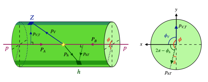
Figure 1: Left: Illustration of TEEC in the $pp$ center-of-mass frame. The incoming proton momentum $P_{A}$ and $P_{B}$ define the $z$-axis. The transverse momentum of the outgoing vector boson $\bm{p}_{V,T}$ defines the $+y$-direction and hence the $xy$-plane is determined. Right: The $xy$-plane of the left panel.

$$p\pqty{P_{A}}+p\pqty{P_{B}}\to V\pqty{p_{V}}+h\pqty{p_{h}}+X\,,$$ (1)

where $p$, $V$ and $h$ denote the initial-state proton, final-state vector boson (either photon or $Z$-boson) and final-state hadron. The momentum of each particle is given in parenthesis. With $E_{T,V}$ and $E_{T,h}$ denoting the transverse energy of the vector boson $V$ and the final-state hadron $h$, we define the TEEC as:

TEEC $$=\sum_{h}\int\differential{\sigma}\frac{E_{T,V}E_{T,h}}{E_{T,V}\sum_{h^{\prime}}E_{T,h^{\prime}}}\delta\pqty{\tau-\frac{1+\cos{\phi}}{2}}$$

$$=\sum_{h}\int\differential{\sigma}\frac{E_{T,h}}{\sum_{h^{\prime}}E_{T,h^{\prime}}}\delta\pqty{\tau-\frac{1+\cos\phi}{2}}\,.$$ (2)

In this definition, the contributions from all the final-state hadrons are summed over. The variable $\tau$ is defined by $\tau\equiv\pqty{1+\cos{\phi}}/2$, where $\phi$ is the azimuthal angle between the vector boson and hadron $h$ in the $xy$-plane as illustrated in Fig. 1. One can easily find that in the back-to-back configuration where $\phi$ approaches $\pi$, $\pi-\phi=\pi-(2\pi-\phi_{h}+\phi_{V})=\phi_{h}-\phi_{V}-\pi$ is a small angle, and $\tau\ll 1$.

The factorization formalism of the TEEC as defined in Eq. 2 is then expressed as:

$$\frac{\differential{\Sigma}}{\differential{\tau}\differential{y_{V}}\differential{p_{V,T}}} =\sum_{a,b,c}\frac{p_{V,T}}{\sqrt{\tau}}\int_{-\infty}^{\infty}\frac{\differential{b}}{2\pi}e^{-2ib\sqrt{\tau}p_{V,T}}\int\differential{y_{c}}H_{ab\to Vc}\pqty{y_{V},p_{V,T},m_{V},\mu}$$

$$\qquad\qquad\qquad\qquad\times x_{a}\,f_{1,a/p}^{(u)}\pqty{x_{a},b,\mu,\frac{\zeta_{a}}{\nu^{2}}}x_{b}\,f_{1,b/p}^{(u)}\pqty{x_{b},b,\mu,\frac{\zeta_{b}}{\nu^{2}}}J_{c}^{(u)}\pqty{b,\mu,\frac{\zeta_{c}}{\nu^{2}}}S_{abc}\pqty{b,\mu,\nu}$$

$$=\sum_{a,b,c}\frac{p_{V,T}}{\sqrt{\tau}}\int_{0}^{\infty}\frac{\differential{b}}{\pi}\cos(2b\sqrt{\tau}p_{V,T})\int\differential{y_{c}}H_{ab\to Vc}\pqty{y_{V},p_{V,T},m_{V},\mu}$$

$$\qquad\qquad\qquad\qquad\times x_{a}\,f_{1,a/p}^{(u)}\pqty{x_{a},b,\mu,\frac{\zeta_{a}}{\nu^{2}}}x_{b}\,f_{1,b/p}^{(u)}\pqty{x_{b},b,\mu,\frac{\zeta_{b}}{\nu^{2}}}J_{c}^{(u)}\pqty{b,\mu,\frac{\zeta_{c}}{\nu^{2}}}S_{abc}\pqty{b,\mu,\nu}\,,$$ (3)

where $y_{V}$ and $p_{V,T}$ denote the rapidity and transverse momentum of the vector boson, respectively. The subscripts $a$, $b$ and $c$ in $H_{ab\to Vc}$ can take a parton species, $q$ for a quark, $\bar{q}$ for an antiquark, and $g$ for a gluon. Here $y_{c}$ is the rapidity of the parton $c$ that initiates the TEEC jet $J_{c}$, and $m_{V}$ is the mass of the produced vector boson. The $y_{c}$ dependence is implicit and will be detailed in Section II.1.

Since the momentum imbalance is along the $x$ axis by definition, we have $\bm{b}\equiv\pqty{b_{x},b_{y}}=\pqty{b,0}$. As a result, the dimensionality of Fourier transform becomes 1 as previously pointed out in, e.g., Li:2020bub ; Fang:2023thw ; Gao:2023ulg . In the factorization formalism, $f_{1,i/p}^{(u)}\pqty{x_{i},b,\mu,\zeta_{i}/\nu^{2}}$ for parton species $i$ is its “unsubtracted” TMD PDF, where $x_{i}$ is the collinear momentum fraction of the parent hadron carried by parton $i$ and $\zeta_{i}$ is the Collins-Soper parameter. It is worth noting that $b$ contains only the $x$-component as dicussed above. The “unsubtracted” TMD PDFs describe energetic radiations of incoming partons in the direction collinear to the incoming protons Boussarie:2023izj .

The hard function $H_{ab\to Vc}\pqty{y_{V},p_{V,T},m_{V},\mu}$ contains the virtual corrections to the underlying partonic process $ab\to Vc$ that can be obtained through matching calculations between QCD and the soft-collinear effective theory (SCET). The wide-angle soft emissions connecting initial and final colored particles $abc$ are encoded in the soft function $S_{abc}\pqty{b,\mu,\nu}$. Finally, $J_{c}^{(u)}\pqty{b,\mu,\zeta_{c}/\nu^{2}}$ is the “unsubtracted” TEEC jet function, which has a close relation with the TMD fragmentation functions, and will be discussed in Section II.3. To arrive at the last line of Eq. 3, we exploited the fact that $f_{1,i/p}^{(u)}$, $S_{abc}$ and $J_{c}^{(u)}$ are all even functions of $b$ (they all depend on $b^{2}$). The TMD PDFs, soft function and TEEC jet function also depend on the renormalization scale $\mu$ and the rapidity renormalization scale $\nu$ Chiu:2012ir . Furthermore, $\zeta_{a,b,c}$ in TMD PDFs or TEEC jet function are the Collins-Soper parameters and will be discussed in Sections II.1 and II.3.

In the rest of this section, we will quantitatively define and discuss in details each ingredient in the factorization formula in Eq. 3.

II.1 Hard function and TMD PDFs

In Eq. 3, $H_{ab\rightarrow Vc}\pqty{y_{V},p_{V,T},\mu}$ is the hard function that describes the partonic scattering process $ab\rightarrow Vc$. The hard function $H_{ab\rightarrow Vc}$ at LO is given as Chien:2019gyf ; Chien:2022wiq :

$$H_{q\overline{q}\to Vg}^{(0)} =\frac{\mathcal{N}_{H}\pqty{N_{c}^{2}-1}}{N_{c}^{2}}\frac{\hat{t}^{2}+\hat{u}^{2}+2\hat{s}m_{V}^{2}}{\hat{t}\hat{u}}\,,$$ (4)

$$H_{qg\to Vq}^{(0)} =-\frac{\mathcal{N}_{H}}{N_{c}}\frac{\hat{s}^{2}+\hat{t}^{2}+2\hat{u}m_{V}^{2}}{\hat{s}\hat{t}}\,,$$ (5)

where $N_{c}$ is number of colors for quarks and the normalization $\mathcal{N}_{H}$ given by:

$$\mathcal{N}_{H}\equiv\frac{2\pi p_{V,T}}{\hat{s}^{2}}\alpha_{s}\alpha_{\mathrm{em}}\alpha_{q}\,.$$ (6)

The mass of vector boson $m_{V}$ for photon is set to zero, i.e., $m_{\gamma}=0~{}\mathrm{GeV}$, while for $Z$ boson $m_{Z}$ is set at $91.1876~{}\mathrm{GeV}$. The fine structure constants $\alpha_{\mathrm{em}}$ used in phenomenological studies are $1/137$ and $1/128$ for $V=\gamma$ and $V=Z$, respectively, and $\alpha_{s}$ is the strong coupling constant. The parameter $\alpha_{q}$ for $\gamma+h$ production is:

$$\alpha_{q}\equiv e_{q}^{2}\,,$$ (7)

where $e_{q}$ denotes the electric charge of the quark. For $Z+h$ production, $\alpha_{q}$ is given by:

$$\alpha_{q}\equiv\frac{1-4\absolutevalue{e_{q}}\sin[2](\theta_{W})+8e_{q}^{2}\sin[4](\theta_{W})}{8\sin[2](\theta_{W})\cos[2](\theta_{W})}\,,$$ (8)

where $\cos{\theta_{W}}=0.88168$. The collinear momentum fractions $x_{a}$ and $x_{b}$ are given by:

$$x_{a} =\frac{1}{\sqrt{s}}\pqty{\sqrt{p_{V,T}^{2}+m_{V}^{2}}e^{y_{V}}+p_{V,T}e^{y_{c}}}\,,$$ (9)

$$x_{b} =\frac{1}{\sqrt{s}}\pqty{\sqrt{p_{V,T}^{2}+m_{V}^{2}}e^{-y_{V}}+p_{V,T}e^{-y_{c}}}\,,$$ (10)

where $\sqrt{s}$ is the center-of-mass energy for the collision. Finally, $\hat{s}$, $\hat{t}$ and $\hat{u}$ appearing in Eqs. 4 and 5 are the partonic Mandelstam variables. To define them, we first list the three relevant partonic processes:

$$q\pqty{p_{a}}+\overline{q}\pqty{p_{b}}\to V\pqty{p_{V}}+g\pqty{p_{c}}\,,$$ (11)

$$q\pqty{p_{a}}+g\pqty{p_{b}}\to V\pqty{p_{V}}+q\pqty{p_{c}}\,,$$ (12)

$$\overline{q}\pqty{p_{a}}+g\pqty{p_{b}}\to V\pqty{p_{V}}+\overline{q}\pqty{p_{c}}\,,$$ (13)

where $q$, $\overline{q}$ and $g$ denote quark, antiquark and gluon, respectively, and $V$ denotes the vector boson. The partonic Mandelstam variables are then defined as:

$$\hat{s}\equiv\pqty{p_{a}+p_{b}}^{2}\,,\quad\hat{t}\equiv\pqty{p_{a}-p_{V}}^{2}\,,\quad\hat{u}\equiv\pqty{p_{b}-p_{V}}^{2}\,.$$ (14)

The NLO hard function used in this paper is given in Chien:2022wiq . Writing down the NLL resummation requires the hard anomalous dimension up to one-loop order Becher:2009th ; Chien:2019gyf :

$$\gamma_{\mu}^{H}\pqty{\alpha_{s}}=-\sum_{i=a,b,c}\gamma_{i}\bqty{\alpha_{s}\pqty{\mu}}$$

$$\quad+\Gamma_{\mathrm{cusp}}\bqty{\alpha_{s}\pqty{\mu}}\Bigg{[}C_{a}\ln(\frac{\hat{u}^{2}}{p_{V,T}^{2}\mu^{2}})+C_{b}\ln(\frac{\hat{t}^{2}}{p_{V,T}^{2}\mu^{2}})$$

$$\qquad\qquad\qquad\qquad+C_{c}\ln(\frac{p_{V,T}^{2}}{\mu^{2}})\Bigg{]}+\order{\alpha_{s}^{2}}\,,$$ (15)

where the cusp anomalous dimensions $\Gamma_{\mathrm{cusp}}$ and non-cusp anomalous dimensions $\gamma_{i}$ are expanded as:

$$\Gamma_{\mathrm{cusp}}\bqty{\alpha_{s}(\mu)} =\sum_{n=1}\Gamma_{n-1}\pqty{\frac{\alpha_{s}}{4\pi}}^{n}\,,$$ (16)

$$\gamma_{i}\bqty{\alpha_{s}(\mu)} =\sum_{n=1}\gamma_{n}^{i}\pqty{\frac{\alpha_{s}}{4\pi}}^{n}\,.$$ (17)

For the expansion we keep the following terms Korchemsky:1987wg ; Becher:2006mr ; Jain:2011xz :

$$\Gamma_{0}^{q} =4\,,\quad\gamma_{0}^{q}=6C_{F}\,,\quad\gamma_{0}^{g}=2\beta_{0}\,,$$ (18)

$$\Gamma_{1} =C_{A}\pqty{\frac{268}{9}-\frac{4\pi^{2}}{3}}-\frac{80}{9}T_{F}n_{f}\,,$$ (19)

where $C_{F}=4/3$, $C_{A}=3$, $T_{F}=1/2$ and $n_{f}$ is the number of flavors. And $\beta_{0}$ is defined as:

$$\beta_{0}\equiv\frac{11}{3}C_{A}-\frac{4}{3}T_{F}n_{f}\,.$$ (20)

Next, we provide a brief overview of the TMD PDFs $f_{1,i/p}^{(u)}\pqty{x_{i},b,\mu,\zeta_{i}/\nu^{2}}$ for an incoming parton $i$. As discussed in Kang:2023oqj , two scales other than $\mu$ are involved in the “unsubtracted” TMD PDFs $f_{1,i/p}^{(u)}\pqty{x_{i},b,\mu,\zeta_{i}/\nu^{2}}$: the Collins-Soper scale $\zeta$ Collins:2011zzd ; Boussarie:2023izj ; Ebert:2019okf and the rapidity renormalization scale $\nu$ Chiu:2012ir . For both quark and gluon TMD PDFs $f_{1,i/p}^{(u)}$, the rapidity divergences can be canceled by subtracting the square root of the standard soft function $S_{n_{i}\cdot\overline{n}_{i}}\pqty{b,L,L_{\nu}}$. Denoted by $n_{i}$ is the light-like directional four-vector of an incoming or outgoing parton moving with a momentum $p_{i}$ defined in Eqs. 12, 11 and 13, and $L$ and $L_{\nu}$ will be defined in Eq. 21. Adopting dimensional regularization in $4-2\epsilon$ space-time dimensions and the rapidity regulator $\eta$ discussed in Chiu:2012ir , the standard soft function is given by Collins:2011zzd ; Kang:2021ffh :

$$S_{n_{i}\cdot\overline{n}_{i}}\pqty{b,L,L_{\nu}} =1-\frac{\alpha_{s}C_{i}}{2\pi}\bigg{[}2\pqty{\frac{2}{\eta}+L_{\nu}}\pqty{\frac{1}{\epsilon}+L}$$

$$\qquad\qquad\qquad-\frac{2}{\epsilon^{2}}+L^{2}+\frac{\pi^{2}}{6}\bigg{]},$$ (21)

where $L\equiv\ln(\mu^{2}/\mu_{b}^{2})$ with $\mu_{b}\equiv 2e^{-\gamma_{E}}/b$, $L_{\nu}\equiv\ln(\nu^{2}/\mu^{2})$, $C_{i}$ takes the value of $C_{F}$ or $C_{A}$ for quark and gluon TMD PDFs, respectively, and $\gamma_{E}$ is the Euler-Mascheroni constant. Using $S_{n_{i}\cdot\overline{n}_{i}}$ from Eq. 21, we additionally define the “subtracted” parton distribution $f_{1,i/p}\pqty{x_{i},b,\mu,\zeta_{i}}$ that is free from the rapidity divergence Collins:2011zzd :

$$f_{1,i/p}\pqty{x_{i},b,\mu,\zeta_{i}} =f_{1,i/p}^{(u)}\pqty{x_{i},b,\mu,\frac{\zeta_{i}}{\nu^{2}}}$$

$$\quad\times\sqrt{S_{n_{i}\cdot\overline{n}_{i}}\pqty{b,L,L_{\nu}}}\,.$$ (22)

The TMD evolution for the “subtracted” TMD PDFs is now given by the Collins-Soper evolution and the renormalization group equation, each associated with the Collins-Soper scale $\zeta$ Collins:2011zzd ; Boussarie:2023izj and the scale $\mu$, respectively. The evolution equations are given by:

$$\frac{\differential{}}{\differential{\ln\sqrt{\zeta}}}\ln{f_{1,i/p}\pqty{x_{i},b,\mu,\zeta}} =K(b,\mu)\,,$$ (23)

$$\frac{\differential{}}{\differential{\ln{\mu}}}\ln{f_{1,i/p}\pqty{x_{i},b,\mu,\zeta_{i}}} =\gamma_{\mu,i}^{f}\bqty{\alpha_{s}(\mu),\frac{\zeta_{i}}{\mu^{2}}}\,,$$ (24)

where $K\pqty{b,\mu}$ denotes the Collins-Soper evolution kernel Collins:2011zzd ; Boussarie:2023izj ; Moult:2022xzt ; Duhr:2022yyp , and $\gamma_{\mu,i}^{f}\bqty{\alpha_{s}(\mu),\zeta_{i}/\mu^{2}}$ is the $\mu$ evolution kernel that evolves $f_{1,i/p}\pqty{x_{i},b,\mu,\zeta_{i}}$ in scale $\mu$ at fixed $\zeta=\zeta_{i}$. Up to two-loop order, $\gamma_{\mu,i}^{f}$ is given by:

$$\gamma_{\mu,i}^{f}\bqty{\alpha_{s}(\mu),\frac{\zeta_{i}}{\mu^{2}}}= -C_{i}\Gamma_{\mathrm{cusp}}\bqty{\alpha_{s}(\mu)}\ln(\frac{\zeta_{i}}{\mu^{2}})$$

$$+\gamma_{i}\bqty{\alpha_{s}(\mu)}\,,$$ (25)

where $C_{i}=C_{F}$ $(C_{A})$ for $i=q$ $(g)$, and $\Gamma_{\mathrm{cusp}}$ and $\gamma_{i}$ are the cusp and non-cusp anomalous dimensions, respectively. They are given in Eqs. 16 and 17.

Solving the renormalization group equations on $\zeta$ and $\mu$ while taking into account the non-perturbative contributions from the large $b\gg 1/\Lambda_{\mathrm{QCD}}$ region, we obtain the expressions for TMD PDFs:

$$f_{1,i/p}\pqty{x_{i},b,\mu,\zeta_{i}}=f_{1,i/p}\pqty{x_{i},b,\mu_{b_{*}},\mu_{b_{*}}^{2}}$$ (26)

$$\quad\times\exp[-S_{\mathrm{NP}}^{i}(b,Q_{0},\zeta_{i})]\exp[-S_{\mathrm{pert}}^{i}(\mu,\mu_{b_{*}},\zeta_{i})]\,,$$

where we evolve the TMD PDFs from initial scales $\pqty{\mu_{0},\zeta_{0}}$ to final scales $\pqty{\mu,\zeta_{i}=\hat{s}}$. We have chosen the following initial scales $\mu_{0}=\sqrt{\zeta_{0}}=\mu_{b_{*}}$. As usual, we define $\mu_{b_{*}}\equiv 2e^{-\gamma_{E}}/b_{*}$ and $b_{*}\equiv b/\sqrt{1+b^{2}/b_{\max}^{2}}$ with $b_{\max}=1.5~{}\mathrm{GeV}^{-1}$ following the $b_{*}$-prescription Echevarria:2020hpy ; Sun:2014dqm ; Isaacson:2023iui ; Collins:1984kg . The choice of $\zeta_{i}=\hat{s}$ for the incoming partons will be discussed in Section II.3. The perturbative Sudakov factor $S_{\mathrm{pert}}^{i}\pqty{\mu,\mu_{b_{*}},\zeta_{i}}$ is given by:

$$S_{\mathrm{pert}}^{i}\pqty{\mu,\mu_{b_{*}},\zeta_{i}} =-K\pqty{b_{*},\mu_{b_{*}}}\ln(\frac{\sqrt{\zeta_{i}}}{\mu_{b_{*}}})$$

$$\quad-\int_{\mu_{b_{*}}}^{\mu}\frac{\differential{\mu^{\prime}}}{\mu^{\prime}}\gamma_{\mu,i}^{f}\bqty{\alpha_{s}(\mu^{\prime}),\frac{\zeta_{i}}{\mu^{\prime 2}}}\,,$$ (27)

and the non-perturbative Sudakov factor for $i=q$ is given by Sun:2014dqm ; Echevarria:2020hpy :

$$S_{\mathrm{NP}}^{i}\pqty{b,Q_{0},\zeta_{i}}=\frac{g_{2}}{2}\ln(\frac{b}{b_{*}})\ln(\frac{\sqrt{\zeta_{i}}}{Q_{0}})+g_{1}^{q}b^{2}\,,$$ (28)

with $Q_{0}^{2}=2.4~{}\mathrm{GeV}^{2}$, $g_{2}=0.84$ and $g_{1}^{q}=0.106~{}\mathrm{GeV}^{2}$. For $i=g$, we will follow Balazs:1997hv ; Balazs:2000wv ; Balazs:2007hr and adopt the following parameterization:

$$S_{\mathrm{NP}}^{i}\pqty{b,Q_{0},\zeta_{i}}=\frac{C_{A}}{C_{F}}\frac{g_{2}}{2}\ln(\frac{b}{b_{*}})\ln(\frac{\sqrt{\zeta_{i}}}{Q_{0}})+g_{1}^{g}b^{2}\,,$$ (29)

where we set $g_{1}^{g}=g_{1}^{q}$. Throughout this paper, we work at the next-to-leading logarithmic (NLL) level in resummation accuracy, where $K\pqty{b_{*},\mu_{b_{*}}}=0$.

In the conventional TMD approach Boussarie:2023izj , one can express $f_{1,i/p}\pqty{x,b,\mu_{b_{*}},\mu_{b_{*}}^{2}}$ in terms of the collinear parton distribution functions through operator product expansion:

$$f_{1,i/p}\pqty{x_{i},\mu_{b_{*}}} =\sum_{j}\int_{x_{i}}^{1}\frac{\differential{x^{\prime}}}{x^{\prime}}C_{i\leftarrow j}\pqty{\frac{x_{i}}{x^{\prime}},\mu_{b_{*}}}f_{j/p}\pqty{x^{\prime},\mu_{b_{*}}}$$

$$\equiv\bqty{C_{i\leftarrow j}\otimes f_{j/p}}\pqty{x_{i},\mu_{b_{*}}}\,,$$ (30)

where we adopt a shorthand notation $f_{1,i/p}\pqty{x_{i},\mu_{b_{*}}}$ for TMD PDFs and $f_{j/p}\pqty{x,\mu}$ denotes the proton collinear parton distribution of flavor $j$. The matching coefficients $C_{i\leftarrow j}$ are perturbatively calculable and can be found in e.g., Aybat:2011zv ; Collins:2011zzd ; Kang:2015msa ; Echevarria:2016scs ; Luo:2019szz ; Echevarria:2020hpy ; Luo:2020epw ; Ebert:2020yqt .

The nuclear modification is considered by substituting the nuclear collinear PDFs $f_{j/A}$ for the vacuum collinear PDFs $f_{j/p}$ in Eq. 30. In this work we adopt the EPPS16 set Eskola:2016oht for both gold (Au) and lead (Pb). For the proton PDFs, we use CT14nlo Dulat:2015mca to be consistent with the choice made in EPPS16. Additionally, we follow the work in Alrashed:2021csd and introduce a modified non-perturbative parameter $g_{1,A}^{q}$ in place of $g_{1}^{q}$ in Eq. 28:

$$g_{1,A}^{q}=g_{1}^{q}+a_{N}L\,,$$ (31)

where $L\equiv A^{1/3}-1$ with $A$ being the mass number of the nucleus. Our choice of nuclear broadening parameter $a_{N}=0.016$ GeV² was determined in Alrashed:2021csd from fitting experimental data using EPPS16 set Eskola:2016oht as the collinear baseline.

II.2 Soft function

The soft function for $V+h$ production can be computed with the rapidity regulator Chiu:2011qc , and the expressions are given by Buffing:2018ggv ; Li:2020bub ; Kang:2023oqj ; Fang:2023thw :

$$S_{abc}\pqty{b,\mu,\nu}=1 -\bm{T}_{a}\cdot\bm{T}_{b}S_{n\cdot\overline{n}}^{\pqty{1}}\pqty{b,L,L_{\nu}+\ln(n_{ab})}$$

$$-\bm{T}_{b}\cdot\bm{T}_{c}S_{n\cdot\overline{n}}^{\pqty{1}}\pqty{b,L,L_{\nu}+\ln(n_{bc})}$$

$$-\bm{T}_{c}\cdot\bm{T}_{a}S_{n\cdot\overline{n}}^{\pqty{1}}\pqty{b,L,L_{\nu}+\ln(n_{ca})}\,,$$ (32)

where $\bm{T}_{a,b,c}$ are color factors, and $S_{n\cdot\overline{n}}^{\pqty{1}}$ is the NLO component defined by the relation $S_{n_{i}\cdot\overline{n}_{i}}=1+C_{i}S_{n\cdot\overline{n}}^{\pqty{1}}$ for the standard soft function given in Eq. 21. We have also defined $n_{ab}\equiv n_{a}\cdot n_{b}/2$.

Using color conservation $\bm{T}_{a}+\bm{T}_{b}+\bm{T}_{c}=0$, we obtain:

$$S_{abc}\pqty{b,\mu,\nu} =1+\frac{1}{2}\pqty{\bm{T}_{a}^{2}+\bm{T}_{b}^{2}+\bm{T}_{c}^{2}}S_{n\cdot\overline{n}}^{\pqty{1}}\pqty{b,L,L_{\nu}}$$

$$-\frac{\alpha_{s}L}{2\pi}\sum_{\mathrm{cyc}}\pqty{\bm{T}_{a}^{2}+\bm{T}_{b}^{2}-\bm{T}_{c}^{2}}\ln(n_{ab})$$

$$-\frac{\alpha_{s}L}{2\pi}\frac{1}{\epsilon}\sum_{\mathrm{cyc}}\pqty{\bm{T}_{a}^{2}+\bm{T}_{b}^{2}-\bm{T}_{c}^{2}}\ln(n_{ab})\,,$$ (33)

where $\bm{T}_{q(g)}^{2}=C_{F}$ $(C_{A})$ and $\sum_{\mathrm{cyc}}$ represents a cyclic summation over the indices $a$, $b$ and $c$.

Next we define the so-called “proper” TMD global soft function which does not depend on the rapidity scale $\nu$:

$$S_{abc}^{g,\mathrm{bare}}(b,\mu)=\frac{1}{\sqrt{S_{n_{a}\cdot\overline{n}_{a}}S_{n_{b}\cdot\overline{n}_{b}}S_{n_{c}\cdot\overline{n}_{c}}}}S_{abc}(b,\mu,\nu)\,.$$ (34)

The renormalized TMD global soft function $S_{abc}^{g}(b,\mu)$ is:

$$S_{abc}^{g}(b,\mu)=1-\frac{\alpha_{s}L}{2\pi}\sum_{\mathrm{cyc}}\pqty{\bm{T}_{a}^{2}+\bm{T}_{b}^{2}-\bm{T}_{c}^{2}}\ln(n_{ab})\,.$$ (35)

The renormalization group equation for $S_{abc}^{g}$ is given as:

$$\frac{\differential{}}{\differential{\ln{\mu}}}\ln{S_{abc}^{g}(b,\mu)}=\gamma_{\mu}^{S}(\alpha_{s})\,,$$ (36)

where the anomalous dimension $\gamma_{\mu}^{S}$ is given by:

$$\gamma_{\mu}^{S}(\alpha_{s})=-\frac{\alpha_{s}}{\pi}\sum_{\mathrm{cyc}}\pqty{\bm{T}_{a}^{2}+\bm{T}_{b}^{2}-\bm{T}_{c}^{2}}\ln(n_{ab})\,.$$ (37)

One can work out the scalar products $n_{ab}$ in the above equation Gao:2023ivm :

$$n_{ab}=1\,,\quad n_{ac}=\frac{-\hat{u}}{\hat{s}-m_{V}^{2}}\,,\quad n_{bc}=\frac{-\hat{t}}{\hat{s}-m_{V}^{2}}\,,$$ (38)

where the partonic Mandelstam variables $\hat{s}$, $\hat{t}$ and $\hat{u}$ are given in Eq. 14.

II.3 TEEC jet function

We have introduced the “unsubtracted” TEEC jet function $J_{c}^{(u)}\pqty{b,\mu,\zeta_{c}/\nu^{2}}$ in Eq. 3. Its relation to the “unsubtracted” transverse momentum dependent fragmentation functions (TMD FFs) is given by Moult:2018jzp :

$$J_{c}^{(u)}\pqty{b,\mu,\frac{\zeta_{c}}{\nu^{2}}}\equiv\sum_{h}\int_{0}^{1}\differential{z}zD^{(u)}_{1,h/c}\pqty{z,b,\mu,\frac{\zeta_{c}}{\nu^{2}}}\,.$$ (39)

Similarly to the TMD PDFs, we define the “subtracted” TMD FFs in such a way that the standard soft function $\sqrt{S_{n_{c}\cdot\overline{n}_{c}}\pqty{b,L,L_{\nu}}}$ cancels out the rapidity divergence:

$$D_{1,h/c}\pqty{z,b,\mu,\zeta_{c}} =D^{(u)}_{1,h/c}\pqty{z,b,\mu,\frac{\zeta_{c}}{\nu^{2}}}$$

$$\quad\times\sqrt{S_{n_{c}\cdot\overline{n}_{c}}\pqty{b,L,L_{\nu}}}\,.$$ (40)

The evolution equation is given by:

$$\frac{\differential{}}{\differential{\ln{\mu}}}\ln{D_{1,h/c}\pqty{z,b,\mu,\zeta_{c}}} =\gamma_{\mu,c}^{J}\bqty{\alpha_{s}(\mu),\frac{\zeta_{c}}{\mu^{2}}}\,,$$ (41)

where $\gamma_{\mu,c}^{J}\bqty{\alpha_{s}(\mu),\zeta_{i}/\mu^{2}}$ is the evolution kernel that governs the $\mu$ scale evolution of $D_{1,h/c}\pqty{z,b,\mu,\zeta_{c}}$ at fixed $\zeta=\zeta_{c}$. Up to two-loop order, $\gamma_{\mu,c}^{J}$ is given by:

$$\gamma_{\mu,c}^{J}\bqty{\alpha_{s}(\mu),\frac{\zeta_{c}}{\mu^{2}}}= -C_{c}\Gamma_{\mathrm{cusp}}\bqty{\alpha_{s}(\mu)}\ln(\frac{\zeta_{c}}{\mu^{2}})$$

$$+\gamma_{c}\bqty{\alpha_{s}(\mu)}\,.$$ (42)

The values of $\zeta_{a}$, $\zeta_{b}$ and $\zeta_{c}$ can be found by demanding RG consistency, i.e.:

$$\gamma_{\mu}^{H}+\gamma_{\mu,a}^{f}+\gamma_{\mu,b}^{f}+\gamma_{\mu}^{S}+\gamma_{\mu,c}^{J}=0\,,$$ (43)

for both $q\overline{q}\to V+g$ and $qg\to V+q$ channels. We find that with the choice $\zeta_{a}=\zeta_{b}=\hat{s}$, and $\zeta_{c}=\pqty{\hat{s}-m_{V}^{2}}^{2}/\hat{s}$, the RG consistency is satisfied for both channels. Subsequently, the corresponding “subtracted” TEEC jet function $J_{c}\pqty{b,\mu,\zeta_{c}}$ can be written as:

$$J_{c}\pqty{b,\mu,\zeta_{c}}\equiv\sum_{h}\int_{0}^{1}\differential{z}zD_{1,h/c}\pqty{z,b,\mu,\zeta_{c}}\,.$$ (44)

The TMD FFs $D_{1,h/c}\pqty{z,b,\mu,\zeta_{c}}$ with QCD evolution are given by:

$$D_{1,h/c}\pqty{z,b,\mu,\zeta_{c}} =\sum_{i}\int_{z}^{1}\frac{\differential{y}}{y}\hat{C}_{i\leftarrow c}\pqty{\frac{z}{y},b}D_{h/i}\pqty{y,\mu_{b_{*}}}$$

$$\quad\times\exp[-S_{\mathrm{pert}}\pqty{\mu,\mu_{b_{*}},\zeta_{c}}]$$

$$\quad\times\exp[-S_{\mathrm{NP}}^{c}\pqty{z,b,Q_{0},\zeta_{c}}]\,,$$ (45)

where $Q_{0}^{2}=2.4~{}\mathrm{GeV}^{2}$, $D_{h/i}$ are the vacuum collinear fragmentation functions (FFs) and the matching coefficients $\hat{C}_{i\leftarrow c}$ can be found in Echevarria:2020hpy ; Luo:2019szz ; Luo:2020epw ; Ebert:2020yqt . The corresponding non-perturbative Sudakov factor $S_{\mathrm{NP}}^{c}\pqty{z,b,Q_{0},\zeta_{c}}$ for quark and gluon are respectively given by Kang:2017glf :

$$S_{\mathrm{NP}}^{q}\pqty{z,b} =\frac{g_{2}}{2}\ln(\frac{b}{b_{*}})\ln(\frac{\sqrt{\zeta_{c}}}{Q_{0}})+g_{1}^{D}\frac{b^{2}}{z^{2}}\,,$$ (46)

$$S_{\mathrm{NP}}^{g}\pqty{z,b} =\frac{C_{A}}{C_{F}}\frac{g_{2}}{2}\ln(\frac{b}{b_{*}})\ln(\frac{\sqrt{\zeta_{c}}}{Q_{0}})+g_{1}^{D}\frac{b^{2}}{z^{2}}\,,$$ (47)

with $g_{2}=0.84$ and $g_{1}^{D}=0.042~{}\mathrm{GeV}^{2}$ Sun:2014dqm ; Echevarria:2020hpy and we have omitted the $Q_{0}$ and $\zeta_{c}$ dependence for brevity.

Following the procedures in Kang:2023oqj , we use the LO matching coefficients $\hat{C}_{i\leftarrow c}\pqty{z,b}=\delta_{ic}\delta\pqty{1-z}$ in Eq. 45 and fit the $z$-integration in Eq. 44 with Li:2021txc ; Kang:2023oqj :

$$\sum_{h}\int_{0}^{1}\differential{z}zD_{h/i}\pqty{z,\mu_{b_{*}}}\exp(-g_{1}^{D}\frac{b^{2}}{z^{2}})$$

$$\equiv\exp[-S_{\mathrm{NP}}^{\mathrm{TEEC}}(b)]\,,$$ (48)

with the functional form:

$$S_{\mathrm{NP}}^{\mathrm{TEEC}}(b)=N_{1}b^{\alpha_{1}}+N_{2}b^{\alpha_{2}}\,.$$ (49)

Here $N_{1}$, $N_{2}$, $\alpha_{1}$ and $\alpha_{2}$ are the fit parameters and their extracted values are given in Table 1. The parameterization chosen here is different from the previous choice made in Kang:2023oqj , since the new parameterization is more flexible and can lead to a successful fit in both vacuum and nuclear environment. As for the choice of collinear FFs that enter Eq. 48, we use the 2021 DSS parameterization Borsa:2021ran for neutral and charged pions, i.e., $\pi^{0}$ and $\pi^{\pm}$. In order to remove the bias from including only pion FFs, we normalize the left-hand side of Eq. 48 by $\sum_{\pi^{0},\pi^{\pm}}\int_{0}^{1}\differential{z}zD_{h/i}\pqty{z,\mu_{b_{*}}}$. Note that in Eq. 49, the same set of parameters in $S_{\mathrm{NP}}^{\mathrm{TEEC}}(b)$ is used for quark and gluon since the sum rule $\sum_{h}\int_{0}^{1}\differential{z}zD_{h/i}(z,\mu_{b_{*}})=1$ holds for $i=q$ and $g$. Additionally, although the FFs for charged and neutral hadrons are currently available in vacuum Borsa:2023zxk , they have not been fitted in nuclear environment yet. We therefore choose to use pion FFs in vacuum, so as to be consistent with the LIKEn pion FFs Zurita:2021kli we used in nuclear environment. We then have the final expressions for the quark and gluon TEEC jet functions:

$$J_{q}\pqty{b,\mu,\zeta_{c}}=\exp[-S_{\mathrm{pert}}\pqty{\mu,\mu_{b_{*}},\zeta_{c}}]$$ (50)

$$\qquad\times\exp[-\frac{g_{2}}{2}\ln(\frac{b}{b_{*}})\ln(\frac{\sqrt{\zeta_{c}}}{Q_{0}})-S_{\mathrm{NP}}^{\mathrm{TEEC}}(b)]\,,$$

$$J_{g}\pqty{b,\mu,\zeta_{c}}=\exp[-S_{\mathrm{pert}}\pqty{\mu,\mu_{b_{*}},\zeta_{c}}]$$ (51)

$$\qquad\times\exp[-\frac{C_{A}}{C_{F}}\frac{g_{2}}{2}\ln(\frac{b}{b_{*}})\ln(\frac{\sqrt{\zeta_{c}}}{Q_{0}})-S_{\mathrm{NP}}^{\mathrm{TEEC}}(b)]\,.$$

As one can expect from the TMD factorization formalism of TMD FFs, the quark and gluon TEEC jet functions are only different by a color factor $C_{A}/C_{F}$ in the non-perturbative Sudakov factor.

The nuclear modification for TEEC jet function is considered following a procedure similar to the one for the TMD PDFs in Section II.1. First we replace the vacuum collinear FFs $D_{h/i}$ in Eq. 45 with the nuclear FFs $D_{h/i}^{A}$. In this work, we use the LIKEn 2021 set Zurita:2021kli for both gold (Au) and lead (Pb). The fitted parameters are summarized in Table 1. Additionally, we follow the work in Alrashed:2021csd and introduce a new parameter $g_{1,A}^{D}$ in place of $g_{1}^{D}$ in Eqs. 46 and 47 such that:

$$g_{1,A}^{D}=g_{1}^{D}+b_{N}L\,,$$ (52)

where $L\equiv A^{1/3}-1$ with $A$ being the mass number of the nucleus, and $b_{N}=0.0097$ GeV² has been determined from fitting experimental data Alrashed:2021csd . See also Ref. Alrashed:2023xsv .

nucleus	$N_{1}$	$N_{2}$	$\alpha_{1}$	$\alpha_{2}$
$p$	0.28	0.45	1.43	0.42
Au	$0.70\pm 0.52$	$0.67\pm 0.52$	$1.15\pm 0.61$	$1.19\pm 0.60$
Pb	$0.53\pm 0.50$	$0.86\pm 0.50$	$1.36\pm 0.58$	$0.98\pm 0.58$

Table 1: The values of fitted parameters from Eq. 49. The values are approximated to the second digits after decimal point. The average values and standard deviation for Au and Pb are calculated from 29 fits corresponding to the Hessian sets given in LIKEn 2021 FFs Zurita:2021kli .

Finally, one can write the factorization formula in Eq. 3 using the “subtracted” TMD PDFs and TEEC jet functions as:

$$\frac{\differential{\Sigma}}{\differential{\tau}\differential{y_{V}}\differential{p_{V,T}}} =\sum_{a,b,c}\frac{p_{V,T}}{\sqrt{\tau}}\int_{0}^{\infty}\frac{\differential{b}}{\pi}\cos(2b\sqrt{\tau}p_{V,T})\int\differential{y_{c}}H_{ab\to Vc}\pqty{y_{V},p_{V,T},m_{V},\mu}$$

$$\qquad\qquad\qquad\qquad\quad\times x_{a}\,f_{1,a/p}\pqty{x_{a},b,\mu,\zeta_{a}}\,x_{b}\,f_{1,b/p}\pqty{x_{b},b,\mu,\zeta_{b}}J_{c}\pqty{b,\mu,\zeta_{c}}S_{abc}^{g}\pqty{b,\mu}\,.$$ (53)

The factorization for $pA$ collision can be obtained by replacing the TMD PDFs and TEEC jet functions with their nuclear counterparts, as discussed before.

In performing phenomenological studies, we choose to evolve the hard function, TMD PDFs, TEEC jet function as well as the soft function to a common scale $\mu=\sqrt{m_{V}^{2}+p_{V,T}^{2}}$ with $m_{V}=91.1876~{}\mathrm{GeV}$ for $Z+h$ and $m_{V}=0~{}\mathrm{GeV}$ for $\gamma+h$. More details on the numerical values of relevant parameters will be discussed in Section III.

III Phenomenology

In this section, we provide numerical predictions for the TEEC using the factorization formula in Eq. 53, both with the RHIC and LHC kinematics. Besides $pp$ collisions, $p\mathrm{Au}$ collisions at RHIC and $p\mathrm{Pb}$ collisions at LHC kinematics are also studied to assess nuclear TMD effects.

First, for the $pp$ collisions at RHIC, we choose $\sqrt{s}=200~{}\mathrm{GeV}$, final-state photon $p_{V,T}\in\pqty{10,20}~{}\mathrm{GeV}$ and rapidity range $y_{V}\in\pqty{-1,1}$, $y_{c}\in\pqty{-1,1}$. This corresponds to the kinematics and detector acceptance at sPHENIX experiment. The predictions for the TEEC in the process $pp\to\gamma+h$ at sPHENIX kinematics are shown in Fig. 2. The cross section decreases with increasing $\tau$, which aligns with expectation, as the final-state photon and hadrons deviate further from the back-to-back configuration as $\tau$ becomes larger, resulting in a lower event count.

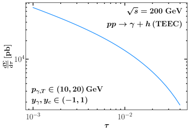
Figure 2: The predictions for the TEEC observable in $pp\to\gamma+h$ at sPHENIX kinematics. Also shown in the figure are the kinematic requirements for photons.

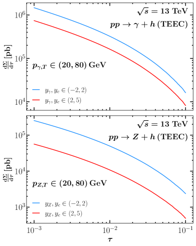
Figure 3: The predictions for the TEEC observable at mid and forward rapidity. In the upper panel, TEEC observable in $pp\to\gamma+h$ at mid (blue) and forward (red) rapidity regions are shown, while in the lower panel, TEEC observable in $pp\to Z+h$ at mid (blue) and forward (red) rapidity regions are presented.

In the upper panel of Fig. 3, we present the same observable in $pp\to\gamma+h$ at LHC energy. We use two rapidity ranges, one with $y_{V,c}\in\pqty{-2,2}$ corresponding to the mid-rapidity, the other one with $y_{V,c}\in\pqty{2,5}$ corresponding to the forward rapidity region. Finally in the lower panel of Fig. 3, we present the predicted $pp\to Z+h$ at LHC energy. A similar trend that was predicted for RHIC is observed here, which again agrees with our expectation. Additionally, the number of events at forward rapidity bin is less than the one at mid-rapidity bin, as expected.

In order to study the nuclear effects, we present the result for $p\mathrm{Au}$ collision at sPHENIX at RHIC and $p\mathrm{Pb}$ collision at LHC. First we define the nuclear modification factor as

$$R_{pA}\equiv\frac{1}{A}\frac{\differential{\Sigma^{pA}}}{\differential{\tau}\differential{y_{V}}\differential{p_{V,T}}}\bigg{/}\frac{\differential{\Sigma^{pp}}}{\differential{\tau}\differential{y_{V}}\differential{p_{V,T}}}\,,$$ (54)

where $A$ in the subscript represents the nuclear target.

For $p\mathrm{Au}$ collision at RHIC, we plot the nuclear modification factor $R_{pA}$ at $\sqrt{s}=200~{}\mathrm{GeV}$, with $p_{T}\in\pqty{10,20}~{}\mathrm{GeV}$ and $y_{\gamma},y_{c}\in\pqty{-1,1}$. This is shown in Fig. 4. The band represents the uncertainties arising from variations in the choice of members from the nuclear collinear FFs Zurita:2021kli . At small $\tau$, a nuclear modification of $\sim 30\%$ can be expected. On the other hand, the nuclear modification approaches or even exceeds 1 as $\tau$ gets larger. This is due to nuclear modification manifesting itself as a broadening effect in the transverse momentum distribution. To be more specific, larger $\tau$ values correspond to larger transverse momentum imbalance between the final-state boson and hadron, and since the transverse momentum gets smeared to larger values in the nuclear environment, the nuclear modification behaves as a suppression effect at smaller $\tau$ and enhancement at larger $\tau$.

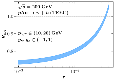
Figure 4: Nuclear modification for $p\mathrm{Au}\to\gamma+h$ at sPHENIX kinematics. The kinematics are labeled in the plots. The band represents the uncertainty from different members of nuclear collinear FFs Zurita:2021kli .

We have also plotted the nuclear modification predictions for the LHC at mid and forward rapidity in Fig. 5. Similar behavior is observed between the RHIC and LHC kinematics. Additionally, when comparing the $R_{pA}$ in the central and forward regions, we find that the $R_{pA}$ values are smaller in the forward rapidity region. This occurs because, in the forward rapidity region, the value of $x_{b}$ (as given in Eq. 10) becomes very small, entering deeper into the shadowing region of nuclear modification. This analysis highlights that the TEEC in $pA$ collisions serves as an excellent observable for studying nuclear modification effects on TMDs. Specifically, the ability to measure a broad range of $\tau$ enables us to study the transverse momentum broadening in the nuclear medium, as encoded in the shape of the $\tau$ distribution. Furthermore, by examining the $\tau$ distribution across different rapidity regions, we can investigate nuclear modification in the collinear parton distribution functions.

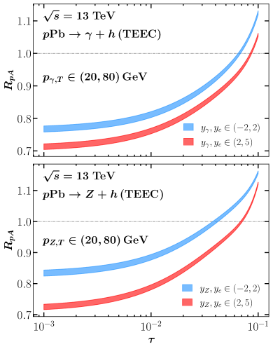
Figure 5: In the upper panel, nuclear modifications for $p\mathrm{Pb}\to\gamma+h$ at mid (blue) and forward (blue) rapidity are shown. In the lower panel, nuclear modifications for $p\mathrm{Pb}\to Z+h$ at mid (blue) and forward (blue) rapidity regions are shown. The kinematic requirements are summarized in the figure. The band represents the uncertainties arising from different choices of members from nuclear collinear FFs Zurita:2021kli .

IV Conclusions

In this paper, we have explored the transverse energy-energy correlator in the $pp$ collision for back-to-back $\gamma$-hadron and $Z$-hadron production at RHIC and the LHC. In the transverse plane, the azimuthal angle difference $\phi$ between the final-state vector boson and the hadron is measured, and we provide a factorization formula for this event-shape observable as $\phi\to\pi$. We present numerical results for TEEC in $pp$ collisions, and find that the TEEC cross section decreases as $\tau$ get larger.

Additionally, we study the nuclear modification in $p\mathrm{Au}$ collision at RHIC and $p\mathrm{Pb}$ collision at LHC. We find that the nuclear modification factor can be $\sim 70\%$ at low $\tau$ region and grows with $\tau$. This observation agrees with our expectation that the nuclear medium broadens the transverse momentum distribution and thus smears the cross section to larger $\tau$ values, or equivalently gives rise to greater transverse momentum imbalance. Furthermore, we investigate the nuclear modification of the TEEC at both central and forward rapidity regions. Our findings indicate that measurements at different rapidities offer valuable insights into the nuclear modification of the collinear component of the TMD in nuclei. This highlights that the TEEC observable serves as an effective probe for studying nuclear modification in TMD physics.

In summary, exploring the transverse energy-energy correlator in vector boson plus hadron production in proton-proton and proton-nucleus collisions presents a fertile ground for studying TMD physics, both in vacuum and nuclear environment. We anticipate the insights obtained from TEEC observables will be crucial in enhancing our understanding of the fundamental aspects of strong interaction physics. We encourage experiments at both RHIC and the LHC to carry out these measurements.

References

- (1) R. Abbate, M. Fickinger, A. Hoang, V. Mateu and I. W. Stewart, Global Fit of to Thrust at N3LL Order with Power Corrections, PoS RADCOR2009 (2010) 040 [arXiv:1004.4894 [hep-ph]].
- (2) A. H. Hoang, D. W. Kolodrubetz, V. Mateu and I. W. Stewart, Precise determination of from the -parameter distribution, Phys. Rev. D 91 (2015) no. 9 094018 [arXiv:1501.04111 [hep-ph]].
- (3) H1 collaboration, V. Andreev et. al., Determination of the strong coupling constant in next-to-next-to-leading order QCD using H1 jet cross section measurements, Eur. Phys. J. C 77 (2017) no. 11 791 [arXiv:1709.07251 [hep-ex]]. [Erratum: Eur.Phys.J.C 81, 738 (2021)].
- (4) A. Banfi, G. P. Salam and G. Zanderighi, Phenomenology of event shapes at hadron colliders, JHEP 06 (2010) 038 [arXiv:1001.4082 [hep-ph]].
- (5) CMS collaboration, V. Khachatryan et. al., First Measurement of Hadronic Event Shapes in Collisions at TeV, Phys. Lett. B 699 (2011) 48 [arXiv:1102.0068 [hep-ex]].
- (6) ATLAS collaboration, G. Aad et. al., Measurement of event shapes at large momentum transfer with the ATLAS detector in collisions at TeV, Eur. Phys. J. C 72 (2012) 2211 [arXiv:1206.2135 [hep-ex]].
- (7) CMS collaboration, S. Chatrchyan et. al., Event Shapes and Azimuthal Correlations in + Jets Events in Collisions at TeV, Phys. Lett. B 722 (2013) 238 [arXiv:1301.1646 [hep-ex]].
- (8) CMS collaboration, V. Khachatryan et. al., Study of Hadronic Event-Shape Variables in Multijet Final States in pp Collisions at = 7 TeV, JHEP 10 (2014) 087 [arXiv:1407.2856 [hep-ex]].
- (9) ATLAS collaboration, G. Aad et. al., Measurement of transverse energy-energy correlations in multi-jet events in collisions at TeV using the ATLAS detector and determination of the strong coupling constant , Phys. Lett. B 750 (2015) 427 [arXiv:1508.01579 [hep-ex]].
- (10) ATLAS collaboration, M. Aaboud et. al., Determination of the strong coupling constant from transverse energy–energy correlations in multijet events at using the ATLAS detector, Eur. Phys. J. C 77 (2017) no. 12 872 [arXiv:1707.02562 [hep-ex]].
- (11) CMS collaboration, A. M. Sirunyan et. al., Event shape variables measured using multijet final states in proton-proton collisions at TeV, JHEP 12 (2018) 117 [arXiv:1811.00588 [hep-ex]].
- (12) ATLAS collaboration, G. Aad et. al., Determination of the strong coupling constant from transverse energyenergy correlations in multijet events at TeV with the ATLAS detector, JHEP 07 (2023) 085 [arXiv:2301.09351 [hep-ex]].
- (13) M. Czakon, A. Mitov and R. Poncelet, Next-to-Next-to-Leading Order Study of Three-Jet Production at the LHC, Phys. Rev. Lett. 127 (2021) no. 15 152001 [arXiv:2106.05331 [hep-ph]]. [Erratum: Phys.Rev.Lett. 129, 119901 (2022), Erratum: Phys.Rev.Lett. 129, 119901 (2022)].
- (14) M. Alvarez, J. Cantero, M. Czakon, J. Llorente, A. Mitov and R. Poncelet, NNLO QCD corrections to event shapes at the LHC, JHEP 03 (2023) 129 [arXiv:2301.01086 [hep-ph]].
- (15) ATLAS collaboration, G. Aad et. al., Measurement of charged-particle event shape variables in TeV proton-proton interactions with the ATLAS detector, Phys. Rev. D 88 (2013) no. 3 032004 [arXiv:1207.6915 [hep-ex]].
- (16) ATLAS collaboration, G. Aad et. al., Properties of jet fragmentation using charged particles measured with the ATLAS detector in collisions at TeV, Phys. Rev. D 100 (2019) no. 5 052011 [arXiv:1906.09254 [hep-ex]].
- (17) ALICE collaboration, S. Acharya et. al., Exploration of jet substructure using iterative declustering in pp and Pb–Pb collisions at LHC energies, Phys. Lett. B 802 (2020) 135227 [arXiv:1905.02512 [nucl-ex]].
- (18) ALICE collaboration, S. Acharya et. al., Measurements of the groomed and ungroomed jet angularities in pp collisions at = 5.02 TeV, JHEP 05 (2022) 061 [arXiv:2107.11303 [nucl-ex]].
- (19) ALICE collaboration, S. Acharya et. al., First measurements of N-subjettiness in central Pb-Pb collisions at = 2.76 TeV, JHEP 10 (2021) 003 [arXiv:2105.04936 [nucl-ex]].
- (20) D. Kang, C. Lee and I. W. Stewart, Using 1-Jettiness to Measure 2 Jets in DIS 3 Ways, Phys. Rev. D 88 (2013) 054004 [arXiv:1303.6952 [hep-ph]].
- (21) Z.-B. Kang, X. Liu and S. Mantry, 1-jettiness DIS event shape: NNLL+NLO results, Phys. Rev. D 90 (2014) no. 1 014041 [arXiv:1312.0301 [hep-ph]].
- (22) H. Cao, Z.-B. Kang, X. Liu and S. Mantry, One-jettiness DIS event shape at N3LL+O(s2), Phys. Rev. D 110 (2024) no. 1 014045 [arXiv:2401.01941 [hep-ph]].
- (23) H1 collaboration, V. Andreev et. al., Measurement of the 1-jettiness event shape observable in deep-inelastic electron-proton scattering at HERA, Eur. Phys. J. C 84 (2024) no. 8 785 [arXiv:2403.10109 [hep-ex]].
- (24) H1 collaboration, V. Andreev et. al., Measurement of groomed event shape observables in deep-inelastic electron-proton scattering at HERA, Eur. Phys. J. C 84 (2024) no. 7 718 [arXiv:2403.10134 [hep-ex]].
- (25) D. Boer et. al., Gluons and the quark sea at high energies: Distributions, polarization, tomography, arXiv:1108.1713 [nucl-th].
- (26) A. Accardi et. al., Electron Ion Collider: The Next QCD Frontier: Understanding the glue that binds us all, Eur. Phys. J. A 52 (2016) no. 9 268 [arXiv:1212.1701 [nucl-ex]].
- (27) R. Abdul Khalek et. al., Science Requirements and Detector Concepts for the Electron-Ion Collider: EIC Yellow Report, Nucl. Phys. A 1026 (2022) 122447 [arXiv:2103.05419 [physics.ins-det]].
- (28) R. Abdul Khalek et. al., Snowmass 2021 White Paper: Electron Ion Collider for High Energy Physics, arXiv:2203.13199 [hep-ph].
- (29) D. E. Kaplan and M. D. Schwartz, Constraining Light Colored Particles with Event Shapes, Phys. Rev. Lett. 101 (2008) 022002 [arXiv:0804.2477 [hep-ph]].
- (30) J. Llorente and B. P. Nachman, Limits on new coloured fermions using precision jet data from the Large Hadron Collider, Nucl. Phys. B 936 (2018) 106 [arXiv:1807.00894 [hep-ph]].
- (31) A. Ali, E. Pietarinen and W. J. Stirling, Transverse Energy-energy Correlations: A Test of Perturbative QCD for the Proton - Anti-proton Collider, Phys. Lett. B 141 (1984) 447.
- (32) C. L. Basham, L. S. Brown, S. D. Ellis and S. T. Love, Energy Correlations in electron - Positron Annihilation: Testing QCD, Phys. Rev. Lett. 41 (1978) 1585.
- (33) C. L. Basham, L. S. Brown, S. D. Ellis and S. T. Love, Energy Correlations in electron-Positron Annihilation in Quantum Chromodynamics: Asymptotically Free Perturbation Theory, Phys. Rev. D 19 (1979) 2018.
- (34) SLD collaboration, K. Abe et. al., Measurement of from hadronic event observables at the resonance, Phys. Rev. D 51 (1995) 962 [arXiv:hep-ex/9501003].
- (35) L3 collaboration, O. Adrian et. al., Determination of alpha-s from hadronic event shapes measured on the resonance, Phys. Lett. B 284 (1992) 471.
- (36) OPAL collaboration, P. D. Acton et. al., An Improved measurement of using energy correlations with the OPAL detector at LEP, Phys. Lett. B 276 (1992) 547.
- (37) TOPAZ collaboration, I. Adachi et. al., Measurements of in Annihilation at GeV and -GeV, Phys. Lett. B 227 (1989) 495.
- (38) TASSO collaboration, W. Braunschweig et. al., A Study of Energy-energy Correlations Between 12-GeV and 46.8-GeV CM Energies, Z. Phys. C 36 (1987) 349.
- (39) JADE collaboration, W. Bartel et. al., Measurements of Energy Correlations in Hadrons, Z. Phys. C 25 (1984) 231.
- (40) E. Fernandez et. al., A Measurement of Energy-energy Correlations in Hadrons at GeV, Phys. Rev. D 31 (1985) 2724.
- (41) D. R. Wood et. al., Determination of From Energy-energy Correlations in Annihilation at GeV, Phys. Rev. D 37 (1988) 3091.
- (42) CELLO collaboration, H. J. Behrend et. al., Analysis of the Energy Weighted Angular Correlations in Hadronic Annihilations at 22 GeV and 34 GeV, Z. Phys. C 14 (1982) 95.
- (43) PLUTO collaboration, C. Berger et. al., A Study of Energy-energy Correlations in Annihilations at .6-GeV, Z. Phys. C 28 (1985) 365.
- (44) OPAL collaboration, M. Z. Akrawy et. al., A Measurement of energy correlations and a determination of in annihilations at GeV, Phys. Lett. B 252 (1990) 159.
- (45) ALEPH collaboration, D. Decamp et. al., Measurement of alpha-s from the structure of particle clusters produced in hadronic Z decays, Phys. Lett. B 257 (1991) 479.
- (46) L3 collaboration, B. Adeva et. al., Determination of alpha-s from energy-energy correlations measured on the resonance., Phys. Lett. B 257 (1991) 469.
- (47) SLD collaboration, K. Abe et. al., Measurement of alpha-s from energy-energy correlations at the resonance, Phys. Rev. D 50 (1994) 5580 [arXiv:hep-ex/9405006].
- (48) ATLAS collaboration, Determination of the strong coupling constant and test of asymptotic freedom from Transverse Energy-Energy Correlations in multijet events at TeV with the ATLAS detector, .
- (49) A. Ali, F. Barreiro, J. Llorente and W. Wang, Transverse Energy-Energy Correlations in Next-to-Leading Order in at the LHC, Phys. Rev. D 86 (2012) 114017 [arXiv:1205.1689 [hep-ph]].
- (50) A. Gao, H. T. Li, I. Moult and H. X. Zhu, Precision QCD Event Shapes at Hadron Colliders: The Transverse Energy-Energy Correlator in the Back-to-Back Limit, Phys. Rev. Lett. 123 (2019) no. 6 062001 [arXiv:1901.04497 [hep-ph]].
- (51) H. T. Li, I. Vitev and Y. J. Zhu, Transverse-Energy-Energy Correlations in Deep Inelastic Scattering, JHEP 11 (2020) 051 [arXiv:2006.02437 [hep-ph]].
- (52) Z.-B. Kang, J. Penttala, F. Zhao and Y. Zhou, Transverse Energy-Energy Correlators in the Color-Glass Condensate at the Electron-Ion Collider, arXiv:2311.17142 [hep-ph].
- (53) CMS collaboration, A. Hayrapetyan et. al., Measurement of Energy Correlators inside Jets and Determination of the Strong Coupling S(mZ), Phys. Rev. Lett. 133 (2024) no. 7 071903 [arXiv:2402.13864 [hep-ex]].
- (54) ALICE collaboration, S. Acharya et. al., Exposing the parton-hadron transition within jets with energy-energy correlators in pp collisions at TeV, arXiv:2409.12687 [hep-ex].
- (55) A. Gao, J. K. L. Michel, I. W. Stewart and Z. Sun, Better angle on hadron transverse momentum distributions at the Electron-Ion Collider, Phys. Rev. D 107 (2023) no. 9 L091504 [arXiv:2209.11211 [hep-ph]].
- (56) Z.-B. Kang, K. Lee, D. Y. Shao and F. Zhao, Probing Transverse Momentum Dependent Structures with Azimuthal Dependence of Energy Correlators, arXiv:2310.15159 [hep-ph].
- (57) ATLAS collaboration, M. Aaboud et. al., Comparison of Fragmentation Functions for Jets Dominated by Light Quarks and Gluons from and Pb+Pb Collisions in ATLAS, Phys. Rev. Lett. 123 (2019) no. 4 042001 [arXiv:1902.10007 [nucl-ex]].
- (58) LHCb collaboration, R. Aaij et. al., Measurement of charged hadron production in -tagged jets in proton-proton collisions at TeV, Phys. Rev. Lett. 123 (2019) 232001 [arXiv:1904.08878 [hep-ex]].
- (59) CMS collaboration, A. Tumasyan et. al., Study of quark and gluon jet substructure in Z+jet and dijet events from pp collisions, JHEP 01 (2022) 188 [arXiv:2109.03340 [hep-ex]].
- (60) LHCb collaboration, Multidifferential study of identified charged hadron distributions in -tagged jets in proton-proton collisions at 13 TeV, Phys. Rev. D 108 (2023) L031103 [arXiv:2208.11691 [hep-ex]].
- (61) A. Gao, H. T. Li, I. Moult and H. X. Zhu, The Transverse Energy-Energy Correlator at Next-to-Next-to-Next-to-Leading Logarithm, arXiv:2312.16408 [hep-ph].
- (62) V. Kartvelishvili, R. Kvatadze and R. Shanidze, On Z and Z + jet production in heavy ion collisions, Phys. Lett. B 356 (1995) 589 [arXiv:hep-ph/9505418].
- (63) X.-N. Wang and Z. Huang, Study medium induced parton energy loss in gamma + jet events of high-energy heavy ion collisions, Phys. Rev. C 55 (1997) 3047 [arXiv:hep-ph/9701227].
- (64) X.-N. Wang, Z. Huang and I. Sarcevic, Jet quenching in the opposite direction of a tagged photon in high-energy heavy ion collisions, Phys. Rev. Lett. 77 (1996) 231 [arXiv:hep-ph/9605213].
- (65) X.-N. Wang and Y. Zhu, Medium Modification of -jets in High-energy Heavy-ion Collisions, Phys. Rev. Lett. 111 (2013) no. 6 062301 [arXiv:1302.5874 [hep-ph]].
- (66) W. Dai, I. Vitev and B.-W. Zhang, Momentum imbalance of isolated photon-tagged jet production at RHIC and LHC, Phys. Rev. Lett. 110 (2013) no. 14 142001 [arXiv:1207.5177 [hep-ph]].
- (67) Z.-B. Kang, I. Vitev and H. Xing, Vector-boson-tagged jet production in heavy ion collisions at energies available at the CERN Large Hadron Collider, Phys. Rev. C 96 (2017) no. 1 014912 [arXiv:1702.07276 [hep-ph]].
- (68) G.-Y. Qin, J. Ruppert, C. Gale, S. Jeon and G. D. Moore, Jet energy loss, photon production, and photon-hadron correlations at RHIC, Phys. Rev. C 80 (2009) 054909 [arXiv:0906.3280 [hep-ph]].
- (69) ATLAS collaboration, M. Aaboud et. al., Measurement of jet correlations in Pb+Pb and collisions at 2.76 TeV with the ATLAS detector, Phys. Lett. B 774 (2017) 379 [arXiv:1706.09363 [hep-ex]].
- (70) CMS collaboration, S. Chatrchyan et. al., Jet Momentum Dependence of Jet Quenching in PbPb Collisions at TeV, Phys. Lett. B 712 (2012) 176 [arXiv:1202.5022 [nucl-ex]].
- (71) ATLAS collaboration, M. Aaboud et. al., Measurement of photon–jet transverse momentum correlations in 5.02 TeV Pb + Pb and collisions with ATLAS, Phys. Lett. B 789 (2019) 167 [arXiv:1809.07280 [nucl-ex]].
- (72) CMS collaboration, A. M. Sirunyan et. al., Study of jet quenching with isolated-photon+jet correlations in PbPb and pp collisions at 5.02 TeV, Phys. Lett. B 785 (2018) 14 [arXiv:1711.09738 [nucl-ex]].
- (73) ATLAS collaboration, M. Aaboud et. al., Measurement of jet fragmentation in Pb+Pb and collisions at TeV with the ATLAS detector, Phys. Rev. C 98 (2018) no. 2 024908 [arXiv:1805.05424 [nucl-ex]].
- (74) CMS collaboration, S. Chatrchyan et. al., Measurement of Jet Fragmentation in PbPb and pp Collisions at TeV, Phys. Rev. C 90 (2014) no. 2 024908 [arXiv:1406.0932 [nucl-ex]].
- (75) S. Fang, W. Ke, D. Y. Shao and J. Terry, Precision three-dimensional imaging of nuclei using recoil-free jets, arXiv:2311.02150 [hep-ph].
- (76) M.-S. Gao, Z.-B. Kang, D. Y. Shao, J. Terry and C. Zhang, QCD resummation of dijet azimuthal decorrelations in pp and pA collisions, JHEP 10 (2023) 013 [arXiv:2306.09317 [hep-ph]].
- (77) R. Boussarie et. al., TMD Handbook, arXiv:2304.03302 [hep-ph].
- (78) J.-Y. Chiu, A. Jain, D. Neill and I. Z. Rothstein, A Formalism for the Systematic Treatment of Rapidity Logarithms in Quantum Field Theory, JHEP 05 (2012) 084 [arXiv:1202.0814 [hep-ph]].
- (79) Y.-T. Chien, D. Y. Shao and B. Wu, Resummation of Boson-Jet Correlation at Hadron Colliders, JHEP 11 (2019) 025 [arXiv:1905.01335 [hep-ph]].
- (80) Y.-T. Chien, R. Rahn, D. Y. Shao, W. J. Waalewijn and B. Wu, Precision boson-jet azimuthal decorrelation at hadron colliders, JHEP 02 (2023) 256 [arXiv:2205.05104 [hep-ph]].
- (81) T. Becher and M. D. Schwartz, Direct photon production with effective field theory, JHEP 02 (2010) 040 [arXiv:0911.0681 [hep-ph]].
- (82) G. P. Korchemsky and A. V. Radyushkin, Renormalization of the Wilson Loops Beyond the Leading Order, Nucl. Phys. B 283 (1987) 342.
- (83) T. Becher, M. Neubert and B. D. Pecjak, Factorization and Momentum-Space Resummation in Deep-Inelastic Scattering, JHEP 01 (2007) 076 [arXiv:hep-ph/0607228].
- (84) A. Jain, M. Procura and W. J. Waalewijn, Parton Fragmentation within an Identified Jet at NNLL, JHEP 05 (2011) 035 [arXiv:1101.4953 [hep-ph]].
- (85) J. Collins, Foundations of Perturbative QCD, vol. 32 of Cambridge Monographs on Particle Physics, Nuclear Physics and Cosmology. Cambridge University Press, 7, 2023.
- (86) M. A. Ebert, I. W. Stewart and Y. Zhao, Towards Quasi-Transverse Momentum Dependent PDFs Computable on the Lattice, JHEP 09 (2019) 037 [arXiv:1901.03685 [hep-ph]].
- (87) Z.-B. Kang, K. Lee, D. Y. Shao and F. Zhao, Spin asymmetries in electron-jet production at the future electron ion collider, JHEP 11 (2021) 005 [arXiv:2106.15624 [hep-ph]].
- (88) I. Moult, H. X. Zhu and Y. J. Zhu, The four loop QCD rapidity anomalous dimension, JHEP 08 (2022) 280 [arXiv:2205.02249 [hep-ph]].
- (89) C. Duhr, B. Mistlberger and G. Vita, Four-Loop Rapidity Anomalous Dimension and Event Shapes to Fourth Logarithmic Order, Phys. Rev. Lett. 129 (2022) no. 16 162001 [arXiv:2205.02242 [hep-ph]].
- (90) M. G. Echevarria, Z.-B. Kang and J. Terry, Global analysis of the Sivers functions at NLO+NNLL in QCD, JHEP 01 (2021) 126 [arXiv:2009.10710 [hep-ph]].
- (91) P. Sun, J. Isaacson, C. P. Yuan and F. Yuan, Nonperturbative functions for SIDIS and Drell–Yan processes, Int. J. Mod. Phys. A 33 (2018) no. 11 1841006 [arXiv:1406.3073 [hep-ph]].
- (92) J. Isaacson, Y. Fu and C. P. Yuan, Improving ResBos for the precision needs of the LHC, arXiv:2311.09916 [hep-ph].
- (93) J. C. Collins, D. E. Soper and G. F. Sterman, Transverse Momentum Distribution in Drell-Yan Pair and W and Z Boson Production, Nucl. Phys. B 250 (1985) 199.
- (94) C. Balazs, E. L. Berger, S. Mrenna and C. P. Yuan, Photon pair production with soft gluon resummation in hadronic interactions, Phys. Rev. D 57 (1998) 6934 [arXiv:hep-ph/9712471].
- (95) C. Balazs and C. P. Yuan, Higgs boson production at the LHC with soft gluon effects, Phys. Lett. B 478 (2000) 192 [arXiv:hep-ph/0001103].
- (96) C. Balazs, E. L. Berger, P. M. Nadolsky and C. P. Yuan, Calculation of prompt diphoton production cross-sections at Tevatron and LHC energies, Phys. Rev. D 76 (2007) 013009 [arXiv:0704.0001 [hep-ph]].
- (97) S. M. Aybat and T. C. Rogers, TMD Parton Distribution and Fragmentation Functions with QCD Evolution, Phys. Rev. D 83 (2011) 114042 [arXiv:1101.5057 [hep-ph]].
- (98) Z.-B. Kang, A. Prokudin, P. Sun and F. Yuan, Extraction of Quark Transversity Distribution and Collins Fragmentation Functions with QCD Evolution, Phys. Rev. D 93 (2016) no. 1 014009 [arXiv:1505.05589 [hep-ph]].
- (99) M. G. Echevarria, I. Scimemi and A. Vladimirov, Unpolarized Transverse Momentum Dependent Parton Distribution and Fragmentation Functions at next-to-next-to-leading order, JHEP 09 (2016) 004 [arXiv:1604.07869 [hep-ph]].
- (100) M.-x. Luo, T.-Z. Yang, H. X. Zhu and Y. J. Zhu, Quark Transverse Parton Distribution at the Next-to-Next-to-Next-to-Leading Order, Phys. Rev. Lett. 124 (2020) no. 9 092001 [arXiv:1912.05778 [hep-ph]].
- (101) M.-x. Luo, T.-Z. Yang, H. X. Zhu and Y. J. Zhu, Unpolarized quark and gluon TMD PDFs and FFs at N3LO, JHEP 06 (2021) 115 [arXiv:2012.03256 [hep-ph]].
- (102) M. A. Ebert, B. Mistlberger and G. Vita, Transverse momentum dependent PDFs at N3LO, JHEP 09 (2020) 146 [arXiv:2006.05329 [hep-ph]].
- (103) K. J. Eskola, P. Paakkinen, H. Paukkunen and C. A. Salgado, EPPS16: Nuclear parton distributions with LHC data, Eur. Phys. J. C 77 (2017) no. 3 163 [arXiv:1612.05741 [hep-ph]].
- (104) S. Dulat, T.-J. Hou, J. Gao, M. Guzzi, J. Huston, P. Nadolsky, J. Pumplin, C. Schmidt, D. Stump and C. P. Yuan, New parton distribution functions from a global analysis of quantum chromodynamics, Phys. Rev. D 93 (2016) no. 3 033006 [arXiv:1506.07443 [hep-ph]].
- (105) M. Alrashed, D. Anderle, Z.-B. Kang, J. Terry and H. Xing, Three-dimensional imaging in nuclei, Phys. Rev. Lett. 129 (2022) no. 24 242001 [arXiv:2107.12401 [hep-ph]].
- (106) J.-y. Chiu, A. Jain, D. Neill and I. Z. Rothstein, The Rapidity Renormalization Group, Phys. Rev. Lett. 108 (2012) 151601 [arXiv:1104.0881 [hep-ph]].
- (107) M. G. A. Buffing, Z.-B. Kang, K. Lee and X. Liu, A transverse momentum dependent framework for back-to-back photon+jet production, arXiv:1812.07549 [hep-ph].
- (108) I. Moult and H. X. Zhu, Simplicity from Recoil: The Three-Loop Soft Function and Factorization for the Energy-Energy Correlation, JHEP 08 (2018) 160 [arXiv:1801.02627 [hep-ph]].
- (109) Z.-B. Kang, X. Liu, F. Ringer and H. Xing, The transverse momentum distribution of hadrons within jets, JHEP 11 (2017) 068 [arXiv:1705.08443 [hep-ph]].
- (110) H. T. Li, Y. Makris and I. Vitev, Energy-energy correlators in Deep Inelastic Scattering, Phys. Rev. D 103 (2021) no. 9 094005 [arXiv:2102.05669 [hep-ph]].
- (111) I. Borsa, D. de Florian, R. Sassot and M. Stratmann, Pion fragmentation functions at high energy colliders, Phys. Rev. D 105 (2022) no. 3 L031502 [arXiv:2110.14015 [hep-ph]].
- (112) I. Borsa, M. Stratmann, D. de Florian and R. Sassot, Charged hadron fragmentation functions at high energy colliders, Phys. Rev. D 109 (2024) no. 5 052004 [arXiv:2311.17768 [hep-ph]].
- (113) P. Zurita, Medium modified Fragmentation Functions with open source xFitter, arXiv:2101.01088 [hep-ph].
- (114) M. Alrashed, Z.-B. Kang, J. Terry, H. Xing and C. Zhang, Nuclear modified transverse momentum dependent parton distribution and fragmentation functions, arXiv:2312.09226 [hep-ph].