Fighting Exponentially Small Gaps by Counterdiabatic Driving

Abstract

We investigate the efficiency of approximate counterdiabatic driving (CD) in accelerating adiabatic passage through a first-order quantum phase transition. Specifically, we analyze a minimal spin-glass bottleneck model that is analytically tractable and exhibits both an exponentially small gap at the transition point and a change in the ground state that involves a macroscopic rearrangement of spins. Using the variational Floquet-Krylov expansion to construct CD terms, we find that while the formation of excitations is significantly suppressed, achieving fully adiabatic evolution remains challenging, necessitating high-order nonlocal terms in the expansion. Our results demonstrate that local CD strategies have limited effectiveness when crossing the extremely small gaps characteristic of NP-hard Ising problems. To address this limitation, we propose an alternative method, termed quantum brachistochrone counterdiabatic driving (QBCD), which significantly increases the fidelity to the target state over the expansion method by directly addressing the gap-closing point and the associated edge states.

I Introduction

The breaking of adiabatic dynamics in many-body spin systems arises in a wide variety of scenarios ranging from condensed matter physics to quantum simulation and quantum computing. According to the adiabatic theorem, the driving of a quantum system in a time shorter than the inverse of the spectral gaps generally induces diabatic transitions. Nonadiabatic dynamics limit the preparation of novel ground-state phases of matter in quantum simulation. Excitations further account for errors in adiabatic quantum computation, quantum annealing, and quantum optimization algorithms. They are also responsible for quantum friction in finite-time thermodynamics, limiting the scaling of quantum heat engines and refrigerators, among other quantum devices.

Enforcing adiabaticity in many-body quantum systems is thus broadly desirable. Yet, it faces the need to overcome small gaps in the spectrum of the driven system. By way of example, hard instances of combinatorial problems might be difficult to solve by quantum annealers because of the presence of gaps on the driving path that are exponentially small in the system size [1, *Young2010First, 3, 4, 5, *Altshuler2010Anderson]. Such gaps render quantum adiabatic evolution unfeasible in practice since the adiabatic theorem requires the driving time $T$ to be larger than the inverse square of the minimal gap $\Delta_{\min}$ [7, 8]. The physical origin of these gaps remains a topic of active debate. Some authors have used perturbation theory to link them to first-order quantum phase transitions [3, 4], suggesting they arise from Anderson localization  [5, 6, 9]. Others argue that the gaps have a non-perturbative origin [10] or result from the clustering of solutions typical in spin-glass phases [11]. Despite the debate, large-scale numerical simulations have consistently demonstrated that certain models display exponentially small gaps [1, *Young2010First, 12, 13].

Facing the presence of small gaps and their dependence on the system size has led to reformulations of the adiabatic theorem in a many-body setting [14, 15], and the notion of quasi-adiabatic continuation used to determine the existence and stability of phases of matter [16, *Hastings2007Quasi, *Hastings2010Locality, *Hastings2010Quasi, 20, 21, 22].

These efforts have been accompanied by a closely related quest for fast quantum control of many-body systems, tackling the presence of small gaps on the adiabatic path. In the context of adiabatic quantum computing, tailoring the mixer or problem Hamiltonian has been proposed to remove the exponential gaps from the path [23, 24, *Choi2011Different, *Choi2011Different2, 27, 28, 29]. Alternative methods involve additional “catalyst” Hamiltonians, i.e., operators that act only at intermediate times to amplify the gap [30, 31, 32, 33, 34, 35, 36, 37, 38, 39]. Other strategies rely on time discretization combined with the use of classical optimization, leading to the quantum approximate optimization algorithm (QAOA) [40, 41], and the use of quantum optimal control to tailor non-linear parameter driving [42, 43, 44, 45, 46].

The problem of speeding up the adiabatic evolution was also addressed in other contexts, such as the application of quantum control in chemistry and physics [47]. Seminal works [48, *Demirplak2005Assisted, *Demirplak2008Consistency, 51] showed that adiabatic evolution for a generic Hamiltonian can be achieved in any finite time, provided an auxiliary counterdiabatic driving (CD) control term is implemented. The CD term is constructed in such a way as to cancel all diabatic transitions, realizing exactly the adiabatic evolution of the reference uncontrolled Hamiltonian. While its explicit form is familiar from early proofs of the adiabatic theorem [52] and can be obtained directly given the spectral decomposition of the instantaneous Hamiltonian, the CD Hamiltonian is generically non-local and involves multiple-body interaction terms  [53, 54, 55, 56]. However, it can also be obtained variationally via controlled expansions in increasingly non-local terms [56, 57, 58, 59, 60, 61], with exact adiabatic dynamics being recovered when all the terms in the expansion are retained. As a result, contrary to catalysts and ad-hoc deformations of the driving Hamiltonian, CD provides a coherent framework to address the problem of exponentially small gaps. CD has been shown to boost the performance of QAOA, motivating its use in quantum optimization  [62, 63, 64, 65, 66, 67, 68]. It should be noted that the required CD terms cannot generally be realized in analog quantum annealers and simulators. However, they can be implemented by digital [53, 56, 62, 63, 66, 69, 70, 67, 68] or hybrid digital-analog quantum simulation [71, 72]. Within such approaches, the implementation is generally facilitated by the locality of the interactions.

Despite a surge of interest in harnessing CD for many-body interacting systems [53, 54, 56, 55, 73, 74, 58, 57, 59, 75, 76, 62, 63, 64, 65, 66, 77, 60, 61, 78, 67], crucial aspects remain to be elucidated. Early studies pointed out the interplay between CD and the Kibble-Zurek (KZ) scaling at second-order quantum phase transitions, which describes the breakdown of adiabaticity while crossing critical point in terms of universal equilibrium critical exponents [79, 80, 81, 82, 83, 84]. It was found that non-local CD terms are needed to suppress the KZ scaling and restore adiabaticity [53, 84, 55], which is at odds with the quest for approximate CD terms with locality tailored for implementations. The breaking of adiabaticity described by KZ mechanism in first-order phase transitions has been theoretically and experimentally studied [85, 86], while the use of bias fields in digitized quantum optimization assisted by CD has only recently been put forward [87]. The performance of CD in a problem with an exponentially small gap and frustration is yet to be elucidated. Some works [88, 89] have addressed the CD-assisted annealing of ferromagnetic $p$-spin models, showing that CD improves the final fidelity while still remaining exponentially small in the system size. The effect of frustration, however, being at the basis of the exponential difficulty of solving NP-hard problems, was not considered. Furthermore, while in certain $p$-spin models, simple antiferromagnetic catalysts can yield a polynomial scaling of the gap [37], this cannot happen if the system is frustrated [39]. A natural question thus arises: how efficiently approximate CD can improve the adiabatic passage through exponentially small gaps induced by frustrated energy levels?

In this work, we study whether local, approximate CD can efficiently tailor excitations for fast-forwarding the adiabatic dynamics in the presence of exponentially small gaps and frustration in many-body quantum systems. To this end, we use the density of non-adiabatic excitations within the framework of the KZ mechanism, well suited for experimental studies [90, 91, 92, 93, 94, 95, 96, 97, 98]. The local approximate CD provides an exponential speed-up of adiabatic dynamics for driving times sufficiently below the adiabatic limit. In addition, we introduce quantum brachistochrone counterdiabatic driving (QBCD) as a complementary approach that leads to a remarkable improvement for near adiabatic time scales, where the local approximate CD loses its efficiency.

I.1 Summary of results

To address the questions above, we study a recently introduced minimal model of a spin-glass bottleneck [99]. The model is an Ising-like spin chain that displays both a small gap and frustration: not only does the gap to the first excited scales exponentially with the system size $L$, but also $O(L)$ spins need to be flipped at the avoided crossing to track adiabatically the ground state. These features are due to a simple localization mechanism reminiscent of the formation of bound states for delta-function potentials on the real line. The model can be mapped onto a chain of free fermions, which allows a complete analytical understanding of the small gap formation [99] and the simulation of large systems to access the asymptotic scaling. We choose to work with this model, and not “standard” NP-hard Hamiltonians as the one for exact cover, as the latter enter the asymptotic scaling for the gap only at prohibitively large system sizes $L\gtrsim 200$ [2], whose dynamics cannot be simulated with present-day classical algorithms.

First of all, we present a thorough analysis of the model properties in Sec. II. While most properties were already derived in the original reference [99], we elucidate the role of a chiral symmetry that was previously mistaken for a regular symmetry and provide a detailed derivation of the free-fermionic representation of the model. Then, after briefly reviewing counterdiabatic driving (CD) in Sec. III.1, we compute the free-fermionic representation of approximate CD for the model under consideration in Sec. III.2.

In Sec. IV, we present our main results. We show that local, approximate CD terms obtained without prior knowledge of the spectrum provide reasonable speed-up only for a given regime of driving times. We do so with two complementary approaches. First, we consider the effect of CD terms on the minimal gap along the adiabatic path, i.e.,  we study the performance of CD as a gap amplification technique. Since the CD Hamiltonian depends on the total evolution time, defining a gap requires care. A solution is presented in Sec. IV.1, showing that if the problem Hamiltonian displays a minimal gap $\Delta_{\min}\sim e^{-\alpha L}$, then adding CD terms leads to $\Delta_{\min{},\mathrm{CD}}\sim e^{-\alpha_{\mathrm{CD}}L}$ with $\alpha_{\mathrm{CD}}$ being smaller than $\alpha$ but remaining finite. Therefore, while CD accelerates the driving protocol exponentially, the scaling remains exponentially hard. Second, in Sec. IV.2, we confirm that CD does not help the system overcome the smallest gap by directly simulating the time evolution of the system. We consider the number of kinks and the excess energy at the end of the schedule, both of which manifest that while CD improves the short-time evolution, it only provides significant improvement for slower schedules when a sufficiently large number of expansion terms are involved. This is because an extensive number of spins need to be flipped, and multiple-body interaction terms are needed to achieve this task. In the language of free fermions, local CD maps to local fermion hopping terms, while a non-local population transfer is needed to track adiabatically the ground state.

In Sec. V, we introduce an alternative approach to the bottleneck problem by attacking directly the first-order phase transition. The QBCD Hamiltonian is constructed using approximate knowledge of the eigenstates at the transition, which remarkably improves the passage through the bottleneck. The QCDB acts by driving the localized edge states associated with the minimal gap. Furthermore, we show that this approach involves a system-size-independent energetic cost for its implementation, as quantified by the Hilbert-Schmidt trace norm. A closing discussion in relation to previous findings follows in Sec. VI.

II Minimal model of spin-glass bottleneck

Consider the quantum many-body Hamiltonian [99]

$$H[\lambda]=-(1-\lambda)\sum_{j=1}^{L}\sigma_{j}^{x}-\lambda\sum_{j=1}^{L}J_{j}\sigma_{j}^{z}\sigma_{j+1}^{z},$$ (1)

where $\lambda\in[0,1]$ is the driving parameter, and the chain has an odd number of sites $L=2\ell+1$, with a periodic boundary. We use square brackets to denote the dependence on the parameter $\lambda$, while we use parentheses for the other functional dependencies, e.g., of $\lambda(t)$ on time. The couplings are set to

$$J_{j}=\begin{cases}J&j=\ell,\ell+1\\ -J^{\prime}&j=2\ell+1\\ 1&\text{otherwise,}\end{cases}$$ (2)

where it is assumed

$$0<J^{\prime}<J<1,\qquad J^{2}<J^{\prime}.$$ (3)

From the pictorial representation in Fig. 1a, it can be seen that Eq. (1) describes an Ising chain with uniform ferromagnetic couplings, except for three weaker couplings placed in diametrically opposite positions: two weak ferromagnetic ones ($J$) next to each other, and one weaker antiferromagnetic one ($-J^{\prime}$) on the other side. The condition $J^{2}<J^{\prime}$ in Eq. (3) is more technical, and is explained in App. B.4.

The Hamiltonian in Eq. (1) has $\mathbb{Z}_{2}$ fermion parity symmetry (the fermionic nature of the parity will become clear in Sec. II.2), due to the possibility of flipping all the spins along $z$:

$$\Pi_{\mathrm{F}}=\prod_{j=1}^{L}\sigma_{j}^{x},\qquad\big{[}\Pi_{\mathrm{F}},H[\lambda]\big{]}=0.$$ (4)

In the following, it will be convenient to restrict to the even parity sector, which is the one dynamically accessible starting from the ground state at $\lambda=0$.

The model has also $\mathbb{Z}_{2}$ reflection parity symmetry $\Pi_{\mathrm{R}}$, defined by the action

$$\Pi_{\mathrm{R}}\sigma_{j}^{\alpha}\Pi_{\mathrm{R}}=\sigma_{L-j+1}^{\alpha},\qquad\alpha=x,y,z,$$ (5)

and highlighted with a grey dashed line in Figs. 1a and 2b. One can check that $\big{[}\Pi_{\mathrm{R}},H[\lambda]\big{]}=0$. It will prove convenient to use a modified version of this symmetry to exploit the free fermionic nature of the chain (see Sec. II.2).

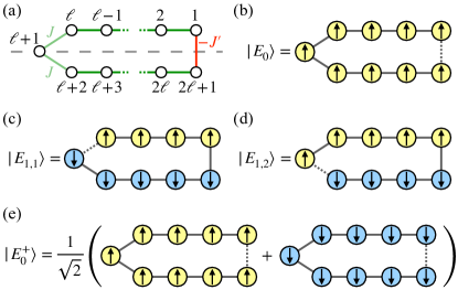
Figure 1: (a) Ising chain of Eqs. (1)–(2). The chain is $L=2\ell+1$ sites long, with uniform ferromagnetic bonds (green lines), except for two neighboring, weakly ferromagnetic bonds (light green lines) and a single antiferromagnetic bond (red line). The dashed gray line indicates the presence of the $\mathbb{Z}_{2}$ reflection symmetries, Eqs. (5) and (10). (b) The ground state at $\lambda=1$ (fixing $L=9$) has only the antiferromagnetic bond frustrated (dotted line). The other degenerate ground state with opposite fermion parity is not shown. (c)–(d) Two degenerate first excited states at $\lambda=1$ (with $L=9$), characterized by only one weak ferromagnetic bond frustrated (dotted line). Two other degenerate first excited states are obtained by flipping all the spins. (e) The restriction to the even fermion parity sector makes the ground state nondegenerate and the first excited manifold two-dimensional. The positive fermion parity states are obtained by means of symmetric combinations, as shown here for the ground state.

II.1 Simple limits

In order to gain an understanding of the model, we analyze the lowest energy states at the beginning ($\lambda=0$) and at the end ($\lambda=1$) of the driving schedule. When $\lambda=0$, the ground state is simply the product state of spins pointing along the $x$ direction, $\ket{E_{0}[\lambda=0]}=\prod_{j}(\ket{\uparrow}_{j}+\ket{\downarrow}_{j})/\sqrt{2}$. It has an even fermionic parity: $\Pi_{\mathrm{F}}\ket{E_{0}[\lambda=0]}=\ket{E_{0}[\lambda=0]}$, since the state on each site is even itself. The $L$ degenerate first-excited states are obtained by flipping one of the spins.

At the end of the driving schedule ($\lambda=1$), because of the presence of a single antiferromagnetic bond in a closed loop geometry, the ground state is frustrated. The condition $0<J^{\prime}<J<1$, Eq. (3), implies that the frustrated bond is at $j=2\ell+1$, see Fig. 1b, and thus the ground-state energy is $E_{0}=-(L-3)-2J+J^{\prime}$. Moreover, because of the fermion parity $\Pi_{\mathrm{F}}$, the ground state is doubly degenerate: the degeneracy is removed by restricting to the even fermion parity sector and taking the symmetric combination $\ket{E_{0}^{+}}$ as in Fig. 1e.

Also the four degenerate first-excited states are easy to determine: they display a single frustrated bond, i.e.,  the weak ferromagnetic link $j=\ell$ or $\ell+1$, and have energies $E_{1}=-(L-3)-J^{\prime}$; see Fig. 1c–d for a pictorial representation (the two other degenerate states are obtained by flipping all the spins). The restriction to the even parity sector implies that symmetric combinations need to be taken, similarly to what is shown in Fig. 1e for the ground state.

From the exact computation reported below, it turns out that at an intermediate value of $\lambda$ the ground state undergoes an exponentially small avoided crossing with the first excited state. In particular, the ground state changes from a dressed version of the states in Fig. 1c–d ($\lambda<\lambda_{c}$) to a dressed version of the state in Fig. 1b ($\lambda>\lambda_{c}$). The ground states before and after the avoided crossing are macroscopically different, as the flipping of half of the chain is involved. Therefore, the Hamiltonian  (1) features a first-order transition similar to the ones that take place in spin-glass models.

The rest of this section is devoted to the analytical description of the avoided crossing of the model. While the computation was already performed in the original work [99], some steps were either missing or wrong (while the final results are substantially correct). For this reason, and to make the manuscript self-contained, we detail the solution and the salient features of the model.

II.2 Fermionic representation and reflection parity symmetry

By means of a Jordan-Wigner transformation, the spin chain Eq. (1) can be fermionized into a chain of Dirac fermions, as detailed in App. A.1. The fermion parity operator $\Pi_{\mathrm{F}}$ in Eq. (4) is transformed into

$$\Pi_{\mathrm{F}}=\prod_{j=1}^{L}\left(1-2c_{j}^{\dagger}c_{j}^{\phantom{\dagger}}\right),$$ (6)

which counts the parity of the total number of fermions. Then, the Hamiltonian is transformed into

$$H[\lambda]=\sum_{j=1}^{L}\left[-\lambda\tilde{J}_{j}\left(c_{j}^{\dagger}-c_{j}^{\phantom{\dagger}}\right)\left(c_{j+1}^{\dagger}+c_{j+1}^{\phantom{\dagger}}\right)\right.\\ \left.+2(1-\lambda)c_{j}^{\dagger}c_{j}^{\phantom{\dagger}}\right]-(1-\lambda)L,$$ (7)

where the couplings $\tilde{J}_{j}$ are the same as $J_{j}$, except that the sign of the last coupling is flipped: $\tilde{J}_{L}=-J_{L}$. This is to take into account the even fermionic parity of the ground state sector; see App. A.1 for a thorough discussion.

Because of the particle non-conservation entailed by the Dirac Hamiltonian (7), it is convenient to pass to the Bogoliubov basis, where excitations are conserved in the adiabatic limit. However, the matrix representation of Eq. (7) is not analytically diagonalizable to the best of our knowledge (see also App. E.1). It is thus convenient to perform two additional transformations [99]. First, each Dirac fermion is split into a couple of Majorana fermions, as illustrated in Fig. 2a, according to:

$$\gamma_{2j-1}:=\frac{1}{\sqrt{2}}\left(c_{j}^{\phantom{\dagger}}+c_{j}^{\dagger}\right),\quad\gamma_{2j}:=\frac{i}{\sqrt{2}}\left(c_{j}^{\phantom{\dagger}}-c_{j}^{\dagger}\right),$$ (8)

that obey commutation relations $\{\gamma_{k},\gamma_{k^{\prime}}\}=\delta_{k,k^{\prime}}$. The Hamiltonian acquires the form

$$H[\lambda]=-2i\sum_{j=1}^{L}\big{[}\lambda\tilde{J}_{j}\gamma_{2j}\gamma_{2j+1}+(1-\lambda)\gamma_{2j-1}\gamma_{2j}\big{]},$$ (9)

see also Fig. 2a and App. A.2. Second, it is convenient to define a modified reflection symmetry $\widetilde{\Pi}_{\mathrm{R}}$, instead of $\Pi_{\mathrm{R}}$ in Eq. (5) (for a detailed explanation see App. A.3). Defining $\widetilde{\Pi}_{\mathrm{R}}$ by the action

$$\widetilde{\Pi}_{\mathrm{R}}\gamma_{k}\widetilde{\Pi}_{\mathrm{R}}=\gamma_{2L-k+1},$$ (10)

one can check that $\widetilde{\Pi}_{\mathrm{R}}^{2}=\mathbb{I}$ and

$$\widetilde{\Pi}_{\mathrm{R}}H[\lambda]\widetilde{\Pi}_{\mathrm{R}}=-H[\lambda],$$ (11)

i.e., that $\widetilde{\Pi}_{\mathrm{R}}$ is a chiral symmetry for $H[\lambda]$. This means that $H[\lambda]$ is not split into sectors and does not acquire a block diagonal form, but simply the spectrum of $H[\lambda]$ is symmetric with respect to $0$, with eigenstates coming in pairs [100].

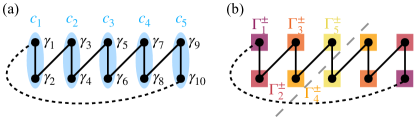
Figure 2: (a) Majorana representation of the chain for $L=5$. Each Dirac site is doubled into two Majorana sites, according to Eq. (8), and thus the length of the Majorana chain becomes $2L$ (i.e., $10$ in the picture). Notice that the sign of the coupling $J_{L}$ between the first and last Majorana fermions is flipped to take into account the even fermionic parity; the bond is dotted in the figure to highlight the fact. (b) Symmetrized Dirac representation of the chain. Each Majorana operator $\gamma_{k}$ is coupled with its symmetric partner $\gamma_{2L-k+1}$, according to Eqs. (12): in the picture, this is shown as a color-code matching of the sites. The chain goes back to a length of $L$ because the sites to the right of the symmetry cut (dashed gray line) become redundant.

The presence of the chiral symmetry $\widetilde{\Pi}_{\mathrm{R}}$ suggests to define the symmetrized operators illustrated in Fig. 2b,

$$\Gamma^{\pm}_{k} =\frac{\pm i\gamma_{k}+\gamma_{2L-k+1}}{\sqrt{2}},\quad k=1,3,\dots,L,$$ (12a)

$$\Gamma^{\pm}_{k} =\frac{\gamma_{k}\pm i\gamma_{2L-k+1}}{\sqrt{2}},\quad k=2,4,\dots,L-1,$$ (12b)

where the factors $\pm i$ where chosen so that

$$\{\Gamma_{k}^{+},\Gamma_{k^{\prime}}^{-}\}=\delta_{k,k^{\prime}},\quad\{\Gamma_{k}^{+},\Gamma_{k^{\prime}}^{+}\}=\{\Gamma_{k}^{-},\Gamma_{k^{\prime}}^{-}\}=0,$$ (13a)

$$\widetilde{\Pi}_{\mathrm{R}}\Gamma_{k}^{\pm}\widetilde{\Pi}_{\mathrm{R}}=\pm i\Gamma_{k}^{\mp},\quad(\Gamma^{\pm}_{k})^{\dagger}=\Gamma^{\mp}_{k}.$$ (13b)

The equations above show that $\Gamma_{k}^{\pm}$ represent a new set of Dirac fermions, in terms of which the Hamiltonian takes the convenient form

$$H[\lambda]= 2\lambda\sum_{j=1}^{\ell}J_{j}\left(\Gamma_{2j}^{+}\Gamma_{2j+1}^{-}+\Gamma_{2j+1}^{+}\Gamma_{2j}^{-}\right)$$ (14)

$$-2(1-\lambda)\sum_{j=1}^{\ell}\left(\Gamma_{2j-1}^{+}\Gamma_{2j}^{-}+\Gamma_{2j}^{+}\Gamma_{2j-1}^{-}\right)$$

$$-\lambda J_{L}\left(2\Gamma_{1}^{+}\Gamma_{1}^{-}-1\right)-(1-\lambda)\left(2\Gamma_{L}^{+}\Gamma_{L}^{-}-1\right),$$

as shown in App. A.4. Above, the $J_{j}$’s have been restored since the last coupling is isolated from the others, and there is no need to keep the $\tilde{J}_{j}$’s. One can check again that $\widetilde{\Pi}_{\mathrm{R}}H[\lambda]\widetilde{\Pi}_{\mathrm{R}}=-H[\lambda]$, as follows immediately from Eqs. (13a)–(13b). Introducing the vectors

$$\vec{\Gamma}^{+}=\begin{pmatrix}\Gamma^{+}_{1}&\Gamma^{+}_{2}&\dots&\Gamma^{+}_{L}\end{pmatrix},\qquad\vec{\Gamma}^{-}=\big{(}\vec{\Gamma}^{+}\big{)}^{\dagger},$$ (15)

and the effective single-particle Hamiltonian

$$\mathcal{H}[\lambda]=\begin{pmatrix}-\lambda J_{L}&\lambda-1&&&&&\\ \lambda-1&0&\lambda J_{1}&&&&\\ &\lambda J_{1}&0&\lambda-1&&&\\ &&\lambda-1&0&\lambda J_{2}&&\\ &&&\lambda J_{2}&\ddots&\ddots&\\ &&&&\ddots&0&\lambda J_{\ell}\\ &&&&&\lambda J_{\ell}&\lambda-1\end{pmatrix},$$ (16)

the matrix representation of the Hamiltonian (14) becomes

$$H[\lambda]=2\,\vec{\Gamma}^{+}\mathcal{H}[\lambda]\vec{\Gamma}^{-}+\lambda J_{L}+(1-\lambda).$$ (17)

From the explicit matrix above, one can see that the diagonalization of $H[\lambda]$ has been reduced to the diagonalization of a simpler one-particle hopping model with open boundary conditions, described by the matrix $\mathcal{H}[\lambda]$. Here and throughout the rest of the paper, we use calligraphic letters to refer to the operators acting on the linear space of the effective Hamiltonian $\mathcal{H}[\lambda]$, and a modified ket notation $|\psi)$ for the corresponding single-particle modes.

II.3 Description of the avoided crossing

The matrix $\mathcal{H}[\lambda]$ in Eq. (16) cannot be diagonalized analytically for general $J_{j}$’s. However, using the $J_{j}$’s given in Eq. (2), all the spectrum can be obtained with a Fourier ansatz: the effective hopping model is translation invariant in the bulk. Thus, the eigenstates must have a plane (or evanescent) wave structure in the bulk, and the effect of the inhomogeneous boundaries can be taken into account by simply fixing the boundary conditions. This is reminiscent of the solution of the Schrödinger equation on a line with a piecewise constant (or delta-function) potential. The computation is carried on in detail in App. B, while here, only the main features are stated.

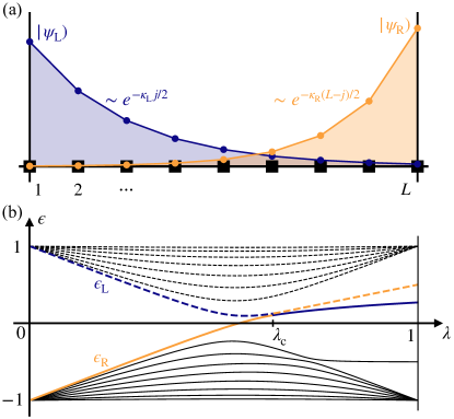
Figure 3: (a) Sketch of the boundary-localized eigenmodes $|\psi_{\mathrm{L}})$,$|\psi_{\mathrm{R}})$ of the effective hopping Hamiltonian (16). (b) Spectrum of the hopping Hamiltonian (16) for $\ell=8$, $J=0.5$, $J^{\prime}=0.27$. The many-body ground state of the $\Gamma$ Hamiltonian in Eq. (14) is formed by populating all the negative-energy modes at $\lambda=0$ (solid lines) and leaving the positive-energy modes empty (dashed lines). The two localized modes $\epsilon_{\mathrm{L}}$ (blue) and $\epsilon_{\mathrm{R}}$ (orange) undergo an avoided crossing at $\lambda=\lambda_{\mathrm{c}}$: while $\epsilon_{\mathrm{R}}$ contributes to the ground state for $\lambda<\lambda_{\mathrm{c}}$ (continuous portion of the orange line), it is replaced by $\epsilon_{\mathrm{L}}$ for $\lambda>\lambda_{\mathrm{c}}$ (the continuous portion of the blue line). Since the spatial overlap between $|\psi_{\mathrm{L}})$ and $|\psi_{\mathrm{R}})$ is exponentially small in $L$, also the gap $\Delta_{\mathrm{min}}$ remains exponentially small according to Eq. (19).

The spectrum of the effective hopping model, Eq. (16), is essentially composed of plane wave eigenmodes. Under the condition $J^{2}<J^{\prime}$. However, a couple of boundary modes are present; see also Eq. (88): one, call it $|\psi_{\mathrm{L}})$, is localized around the left end $j=0$ of the $\Gamma$ chain, and a second one, denoted by $|\psi_{\mathrm{R}})$, extends around the right end $j=L$. Their spatial decay is regulated by the rates $\kappa_{\mathrm{L}}$ and $\kappa_{\mathrm{R}}$ as

$$\psi_{\mathrm{L},j}\sim e^{-\kappa_{\mathrm{L}}j/2},\qquad\psi_{\mathrm{R},j}\sim e^{-\kappa_{\mathrm{R}}(L-j)/2};$$ (18)

see Fig. 3a for a sketch. The corresponding eigenvalues $\epsilon_{\mathrm{L}}$ and $\epsilon_{\mathrm{R}}$ undergo an avoided crossing at a value of the driving parameter $\lambda=\lambda_{\mathrm{c}}$, with a gap

$$\Delta_{\mathrm{min}}\propto e^{-\alpha L},\qquad\alpha=\frac{1}{2}\ln\left[\frac{J^{\prime}(1-J^{2})}{J^{2}-(J^{\prime})^{2}}\right].$$ (19)

Notice that $\alpha>0$, thanks to the conditions Eq. (3). The exponentially small gap $\Delta_{\mathrm{min}}$ hinders adiabatic driving because the many-body ground state of the spin chain contains the single-particle orbital $|\psi_{\mathrm{R}})$ for $\lambda\lesssim\lambda_{\mathrm{c}}$, while it contains the single-particle orbital $|\psi_{\mathrm{L}})$ for $\lambda\gtrsim\lambda_{\mathrm{c}}$, see Fig. 3b. Therefore, the minimal gap along the adiabatic path is equal to $\Delta_{\mathrm{min}}$. At the avoided crossing, it is necessary to bring an effective particle from one end of the $\Gamma$ chain to the other end: in the language of spins, this corresponds to flipping an extensive number of them.

III Counterdiabatic driving

III.1 Brief review of counterdiabatic driving

The adiabatic theorem of quantum mechanics guarantees that the quantum dynamics, generated by a time-dependent Hamiltonian $H[\lambda(t)]$, tracks its instantaneous eigenstates, provided that variations in time are slow enough. The adiabaticity condition reads

$$\dot{\lambda}\,\frac{|\bra{m[\lambda(t)]}\partial_{\lambda}H[\lambda(t)]\ket{n[\lambda(t)]}|}{(E_{n}[\lambda(t)]-E_{m}[\lambda(t)])^{2}}\ll 1,$$ (20)

where $\ket{n[\lambda]}$ are the instantaneous eigenstates and $E_{n}[\lambda]$ the corresponding energies. If the condition above is met, then transitions between eigenstates are suppressed [52]; see as well Refs. [7, 8] for refinements on the adiabaticity condition. Yet, a perfect adiabatic tracking can be obtained at any finite driving rate, if the dynamics is generated by the modified counterdiabatic driving (CD) Hamiltonian [48, *Demirplak2005Assisted, *Demirplak2008Consistency, 51]

$$H_{\mathrm{CD}}(t)=H[\lambda(t)]+\partial_{t}\lambda\cdot H_{1}[\lambda(t)],$$ (21)

with

$$H_{1}[\lambda] =i\sum_{n}\big{(}\outerproduct{\partial_{\lambda}n}{n}-\innerproduct{n}{\partial_{\lambda}n}\outerproduct{n}{n}\big{)}$$ (22)

$$=i\sum_{n}\sum_{m\neq n}\frac{\ket{m}\bra{m}\partial_{\lambda}H\ket{n}\bra{n}}{E_{n}-E_{m}},$$ (23)

where the last equation assumes that the spectrum of $H[\lambda(t)]$ is nondegenerate [51]. The first term on the right-hand side of $H_{1}[\lambda]$ is the generator of parallel transport familiar from proofs of the adiabatic theorem. The second term, being diagonal in the instantaneous eigenbasis, provides the correct Berry phase associated with a perfectly adiabatic trajectory [101].

The challenge in utilizing the CD Hamiltonian, such as the one in Eq. (22), comes from the fact that the terms involved are highly non-local and multiple-body, being $\outerproduct{\partial_{\lambda}n}{n}$ similar in structure to a projector [53]. For this reason, a growing body of works has been investigating the possibility of truncating the CD Hamiltonian to few-body local terms while retaining the suppression of diabatic transitions [53, 54, 56, 55, 58, 59, 76, 77]. A convenient framework to this end relies on the Floquet-Krylov expansion of the CD term [59, 60, 61]. Using the equivalent representation

$$H_{1}[\lambda]=-\int_{0}^{+\infty}dx\,e^{-\epsilon|x|}\,e^{ixH[\lambda]}\partial_{\lambda}H[\lambda]e^{-ixH[\lambda]}$$ (24)

with $\epsilon=0^{+}$, one can expand the integrand in powers of $x$ and find, upon integration,

$$H_{1}[\lambda]=i\sum_{n=1}^{\infty}\alpha_{n}\underbrace{[H,\cdots,[H}_{2n-1\text{ times}},\partial_{\lambda}H]\cdots].$$ (25)

Here, $\alpha_{n}=(-1)^{n}\epsilon^{-2n}$ is formally diverging, but allowing the $\alpha_{n}$’s to be free variational parameters, one obtains a controlled expansion of the CD term with increasingly non-local operators [59]. To fix the parameters $\alpha_{n}$, one may either employ a QAOA-inspired procedure, in which they are updated recursively by using as cost function the energy at the end of the driving process [102, 62, 63, 64], or an a priori method like the minimization of the action [58]

$$\mathcal{S}(H_{1}):=\Tr\big(G^{\dagger}(H_{1})G(H_{1})\big{missing}),$$ (26)

where

$$G(H_{1}):=\partial_{t}H[\lambda(t)]-i[H[\lambda(t)],H_{1}],$$ (27)

with respect to the parameters $\alpha_{n}$. We choose to follow the second route since it allows for greater analytical control and does not rely on heavy numerical optimization.

III.2 Approximate counterdiabatic driving for the spin-glass bottleneck model

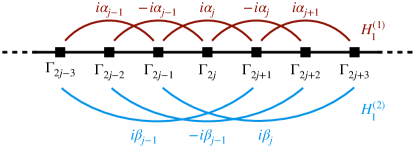
Figure 4: The local approximate counterdiabatic Hamiltonians $H_{1}^{(1)}$, Eq. (28), and $H_{1}^{(2)}$, Eq. (30), take a simple form in the $\Gamma$ free fermionic representation, Eq. (14): they are a longer-range hopping terms, with fine-tuned coefficients $i\alpha_{j},i\beta_{j}$. Higher-order variational ansatzes yield a similar structure with longer-range couplings.

Following Refs. [58, 59], consider the lowest-order approximant to the CD term in the Floquet-Krylov expansion. At the first order, the commutator $[H,\partial_{\lambda}H]$, with $H$ in Eq. (1), contains terms $\sigma_{j}^{y}\sigma_{j+1}^{z}+\sigma_{j}^{z}\sigma_{j+1}^{y}$, motivating the variational ansatz

$$H_{1}^{(1)}[\lambda]=\sum_{j=1}^{L}\alpha_{j}\left(\sigma_{j}^{y}\sigma_{j+1}^{z}+\sigma_{j}^{z}\sigma_{j+1}^{y}\right).$$ (28)

The coefficients $\alpha_{j}$ can be found by minimizing the action (26). This yields the equations

$$\left[8(1-\lambda)^{2}+\lambda^{2}\left(J_{j-1}^{2}+2J_{j}^{2}+J_{j+1}^{2}\right)\right]\alpha_{j}\\ +2\lambda^{2}J_{j}\left(J_{j-1}\alpha_{j-1}+J_{j+1}\alpha_{j+1}\right)=-J_{j},$$ (29)

with periodic boundary conditions implied, which can be solved via linear algebra techniques with a cost polynomial in $L$. Going to the second order, from the computation of the nested commutator $[H,[H,[H,\partial_{\lambda}H]]]$ one determines the variational ansatz $H_{1}^{(1)}[\lambda]+H_{1}^{(2)}[\lambda]$, where

$$H_{1}^{(2)}[\lambda]=\sum_{j=1}^{L}\beta_{j}\left(\sigma_{j}^{y}\sigma_{j+1}^{x}\sigma_{j+2}^{z}+\sigma_{j}^{z}\sigma_{j+1}^{x}\sigma_{j+2}^{y}\right).$$ (30)

Again, the coefficients $\{\alpha_{j},\beta_{j}\}$ can be determined by solving a $2L\times 2L$ linear system (Eq. (106)). Generalizing, one needs to solve a $nN\times nN$ linear system for the $n$-th order term of the Floquet-Krylov expansion. Thus, for finite $n$, the CD term can be determined efficiently with the help of a classical computer.

At all orders of the Floquet-Krylov expansion of the CD Hamiltonian, Eq. (25), the approximate CD term for the spin-glass bottleneck model admits a free-fermionic representation. The full derivation is reported in App. C, and it leads to

$$H_{1}^{(1)}[\lambda] =-2i\sum_{j=1}^{L}\tilde{\alpha}_{j}\left[c^{\dagger}_{j}c^{\dagger}_{j+1}+c_{j}c_{j+1}\right],$$ (31)

$$H_{1}^{(2)}[\lambda] =-2i\sum_{j=1}^{L}\tilde{\beta}_{j}\left[c^{\dagger}_{j}c^{\dagger}_{j+2}+c_{j}c_{j+2}\right].$$ (32)

Notice that the CD terms take the form of longer-range hoppings. A similar longer-range-hopping form is acquired in the $\Gamma_{j}^{\pm}$ basis as well, see Eqs. (104) and (110). Thus, CD helps the driving by preventing localization with two-fermion longer-range hopping terms; see also Sec. VI for further discussion.

IV Results

Here, we present our main results regarding the behavior of CD in the quantum driving of the spin-glass bottleneck model. While the Hamiltonian in Eq. (1) could be studied fully analytically, the introduction of the approximate CD terms forces one to resort to numerical methods: the variational equations (29) and (106) do not seem to have an explicit analytical solution in the general case. Nevertheless, the simple structure of the model, together with the mappings to $c$ and $\Gamma$ fermions performed above, allows for a thorough understanding of the effect of CD on the driving process.

IV.1 Counterdiabatic driving and gap amplification

According to the adiabatic theorem, adiabaticity can be preserved upon reducing the driving time, provided that the gap is increased by the same factor. However, the construction of the CD term outlined in Sec. III.1 indicates that CD is more than a mere gap amplification method: the operators involved are constructed in such a way to transport a state along its adiabatic path, and they do so by enforcing parallel transport while accounting the corresponding quantum phase. By contrast, catalysts and gap-amplifying terms  just enhance the dephasing due to highly oscillatory terms $e^{i(E_{m}-E_{n})t}$ for $m\neq n$, making the adiabatic approximation hold to a better degree [30, 31, 32, 33, 34, 35, 36, 37, 38, 39].

Notice that using a schedule $\lambda(t)$ with vanishing derivative at the endpoints, the eigenstates of $H_{\mathrm{CD}}[\lambda(t)]$, Eq. (21), coincide with those of $H[\lambda(t)]$ at the beginning ($\lambda(0)=0$) and the end ($\lambda(T)=1$) of the protocol. Therefore, when using approximate CD, one can apply the adiabatic theorem to the dynamics generated by $H_{\mathrm{CD}}[\lambda(t)]$ and try to infer the success of the driving process from the minimal gap $\Delta_{\mathrm{min,CD}}$ along the path (by construction, the exact CD term yield success with probability 1 and this study would not make sense there). Noticing that the approximate $H_{\mathrm{CD}}$ depends on the final time $T$, one cannot blindly use the adiabaticity condition to estimate the time $T_{\mathrm{ad}}$ needed for adiabaticity to hold. Nevertheless, it can be used to determine self-consistently $T_{\mathrm{ad}}$, if the dependence $\Delta_{\mathrm{min,CD}}=\Delta_{\mathrm{min,CD}}(T)$ is known.

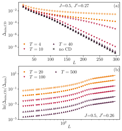
Figure 5: Gap amplification from counterdiabatic driving (CD). (a) For any driving rate, the minimal gap $\Delta_{\mathrm{min,CD}}$ along the CD-assisted adiabatic path remains exponentially small in the system size, both for the 1st order (Eq. (28), filled markers) and 2nd order (Eq. (30), empty markers) variational ansatzes. The bare minimal gap $\Delta_{\mathrm{min}}$ is shown for comparison with black crosses. (b) The CD-assisted gap $\Delta_{\mathrm{min,CD}}$, despite being exponentially small in the system size, is still exponentially larger than the bare gap $\Delta_{\mathrm{min}}$: all the log-log fits (lines) are compatible with a growth $\Delta_{\mathrm{min,CD}}\sim\Delta_{\mathrm{min}}e^{c(T)L}$, with $c(T)=\alpha-\alpha_{\mathrm{CD}}(T)$.

In Fig. 5, the numerical results for the gap $\Delta_{\mathrm{min,CD}}(T)$ of the CD Hamiltonian are shown. The cubic ramp $\lambda(t)=3(t/T)^{2}-2(t/T)^{3}$, that satisfies $\dot{\lambda}(0)=\dot{\lambda}(T)=0$, is used. From Fig. 5a, one can see that, for large system sizes and long driving times, the minimum of the gap remains exponentially small in the system size: $\Delta_{\mathrm{min,CD}}\propto e^{-\alpha_{\mathrm{CD}}L}$. From Fig. 5b, however, one can notice that $\Delta_{\mathrm{min,CD}}$ is still exponentially larger than $\Delta_{\mathrm{min}}$, as a function of the system size $L$ and for every fixed time $T$. In other words, $\alpha_{\mathrm{CD}}<\alpha$. Also, there is no appreciable difference in the values of $\alpha_{\mathrm{CD}}$ extracted from either the first- or second-order expansions; only the prefactor of the exponential is larger for the second-order one.

From plots like that in Fig. 5a, the exponential decay rate $\alpha_{\mathrm{CD}}$ of $\Delta_{\mathrm{min,CD}}$ is extracted for many values of $T$, and the values are reported in Fig. 6. The fits are performed on the first-order expansion gaps; quantitatively similar results follow from using the second-order expansion gaps. One can see that already the first-order ansatz is sufficient to provide an exponential speed-up for moderate driving times, $T\lesssim 25$, as $\alpha_{\mathrm{CD}}$ is substantially smaller than $\alpha$. Increasing the driving time, however, $\alpha_{\mathrm{CD}}$ approaches $\alpha$: higher order CD terms would be required to maintain the same gap amplification.

The conclusion above can be put on quantitative grounds by estimating the adiabatic timescale for approximate CD with the inverse of the minimal gap, $T_{\mathrm{ad,CD}}\sim\Delta^{-2}_{\mathrm{min,CD}}(T)$. Using $\Delta_{\mathrm{min,CD}}(T)\simeq\Delta_{0}e^{-\alpha_{\mathrm{CD}}(T)L}$, with $\alpha_{\mathrm{CD}}(T)\simeq\alpha-\delta/T^{2}$ that is shown to hold up to high precision in Fig. 6b ($\Delta_{0}$ and $\delta$ are two fitting coefficients), one obtains

$$T_{\mathrm{ad,CD}}\approx T_{\mathrm{ad}}\,e^{-2\delta L/T^{2}_{\mathrm{ad,CD}}}\approx T_{\mathrm{ad}}\left(1-\frac{2\delta L}{T^{2}_{\mathrm{ad}}}\right),$$ (33)

where in the last step we expanded up to first order the exponential and approximated $T_{\mathrm{ad,CD}}$ with $T_{\mathrm{ad}}$. One can see that the solution $T_{\mathrm{ad,CD}}$ is significantly reduced for moderate driving times, and it converges to the bare value, $T_{\mathrm{ad}}$, upon increasing $T$. Let us remark that both this empirical power law and the coefficients are expected to change in the favour of smaller adiabatic times for larger order expansions.

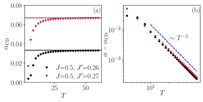
Figure 6: The approximate CD path displays a minimal gap $\Delta_{\mathrm{min,CD}}\propto e^{-\alpha_{\mathrm{CD}}(T)L}$. (a) Rate $\alpha_{\mathrm{CD}}$ as a function of the driving time $T$: the value of $\alpha_{\mathrm{CD}}$ (dots) saturates at the analytical value $\alpha$ in the absence of CD in Eq. (19) (solid lines), already for moderately short times. (b) The approach to the asymptotic value is well fitted by a power law: $\alpha-\alpha_{\mathrm{CD}}(T)\sim T^{-2}$.

IV.2 Performance of counterdiabatic driving

Above, the adiabatic theorem was used to predict the performance of approximate CD. It was found that the gap remains exponentially small in the system size for all driving times, with the gain of CD being less and less significant as the driving time increases. In order to quantify precisely to what extent CD helps the driving process, however, we next integrate the time-dependent Schrödinger equation and see whether the success probability is actually increased.

As before, a cubic ramp $\lambda(t)=3(t/T)^{2}-2(t/T)^{3}$, satisfying $\dot{\lambda}(0)=\dot{\lambda}(T)=0$, is employed. Upon initializing the system in the paramagnetic ground state of $H[\lambda=0]$, we consider the evolution with the approximate CD Hamiltonians $H[\lambda(t)]+\dot{\lambda}(t)H^{(1)}[\lambda(t)]$ (first order ansatz) or $H[\lambda(t)]+\dot{\lambda}(t)[H^{(1)}[\lambda(t)]+H^{(2)}[\lambda(t)]]$ (second order ansatz). Because of the free-fermionic nature of the model under consideration, we evolve the single-particle operators $(c_{j}^{\phantom{\dagger}},c_{j}^{\dagger})$ or $\Gamma_{k}^{\pm}$ by means of Bogoliubov-de Gennes equations, and then compute the desired expectation values at the end of the protocol with the appropriate contractions; see App. E for all the details. This technique allows one to reach much larger system sizes, which are needed in the present case to extract the asymptotic scalings. Incidentally, this is the reason why we employ the chain in Eq. (1) instead of examples of NP-hard Ising Hamiltonians [103].

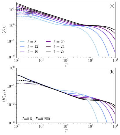
Figure 7: Approximate CD performance measured by the expectation value of the kink number on the final state: $\expectationvalue{K}_{T}\equiv\expectationvalue{K}{\psi(T)}$, Eq. (34). (a) The kink number decreases until it reaches the plateau unit value, corresponding to a single frustrated bond. A driving time exponentially large in the system size is needed to make $\expectationvalue{K}_{T}<1$ and enter the adiabatic regime. The effect of approximate CD is to reduce the kink number at smaller driving times (dashed lines: 1st order ansatz; dotted lines: 2nd order ansatz) with respect to the bare driving with only the Hamiltonian (solid lines). (b) Rescaling the kink number with the system size, a good collapse is obtained at short times, signaling that approximate CD is improving $\expectationvalue{K}_{T}$ by an extensive amount. However, the smallest exponential gap remains as hard to be crossed as for the bare dynamics without CD terms.

The results of our numerical simulations to assess the performance of the driving are presented in Figs. 7–8. First, we compute the kink number in Fig. 7, i.e., the number of frustrated bonds at the end of the process. It is given by the expectation value on the final state of the operator

$$K:=\frac{1}{2}\sum_{j=1}^{L}\left[1-\mathrm{sign}(J_{j})\sigma_{j}^{z}\sigma_{j+1}^{z}\right].$$ (34)

This is an extensive observable that can be computed with free-fermion techniques; the details are shown in App. E.3. From Fig. 7a, one can see that the bottleneck of adiabaticity is represented by one remaining frustrated bond, corresponding to the transition $|\psi_{\mathrm{R}})\to|\psi_{\mathrm{L}})$. The time needed to anneal this last bond gets longer with increasing system size, as indicated by the increasing length of the plateau of $\expectationvalue{K}_{T}\equiv\expectationvalue{K}{\psi(T)}$. From Fig. 7b, one can see instead that the effect of CD is to improve the short-time performance, with a gain that is extensive in the system size. Also, the higher the order of the variational CD ansatz, the bigger the gain. However, one can see that enhancing adiabaticity across the exponentially small gap remains a challenging task for these low-order approaches, and higher-order terms would be required to gain reasonable improvement.

The findings of Fig. 7 agree with the known results about the Kibble-Zurek (KZ) density of defects formed upon crossing a quantum phase transition [79, 80, 81, 82, 83]. The collapse in Fig. 7b shows that the defect density scales as $\sim T^{-\nu/(1+z\nu)}=T^{-1/2}$, where $\nu=1$ is the correlation length exponent of the transverse-field Ising model and $z=1$ is its dynamical exponent. The presence of the three weak links manifests only in the breakdown of the KZ scaling at large times, with the formation of the plateau. The breakdown of the KZ scaling at short times, due to the introduction of approximate CD terms, confirms the early results of Ref. [53] in this setting.

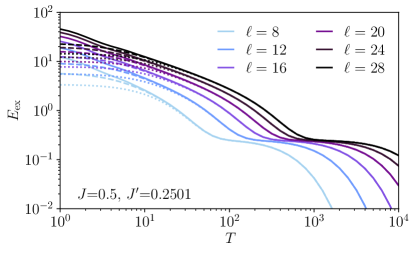
Figure 8: The excess energy in Eq. (35) shares the behavior with the kink number, Eq. (34): the 1st order (Eq. (28), dashed lines) and 2nd order (Eq. (30), dotted lines) variational CD ansatzes improve the driving for short times, but do not help significantly the dynamics to overcome the exponentially small gap. See also Fig. 7 for a comparison.

The same physical picture is confirmed by the excess energy at the end of the protocol, defined by

$$E_{\mathrm{ex}}:=\expectationvalue{H[\lambda=1]}{\psi(T)}-E_{\mathrm{GS}}[\lambda=1]$$ (35)

and shown in Fig. 8a. Thus, figures  7 and 8 demonstrate that CD improves fast driving at short times but does not help significantly to overcome the exponentially small gap, as further discussed in Sec. VI.

V Quantum Brachistochrone Counterdiabatic Driving (QBCD): exponential speedup

In this section, we show how the efficiency of the driving can be improved beyond the low-order CD expansions by canceling the transitions between the ground state and the first excited state around the critical point $\lambda=\lambda_{c}$. Above, the first- and second-order ansatzes were used without requiring any knowledge of the instantaneous spectral properties. Here, an approximate knowledge of the spectrum at a single point in parameter space is assumed, and much better results are obtained. This approach is reminiscent of reverse quantum annealing, where an approximate ground state of the problem Hamiltonian is used to improve the performance of the adiabatic algorithm [104, 105, 106]. Further, this approach differs from the early approaches to CD in many-body systems, where the exact CD term was truncated according to the locality of operators involved [53, 56]. Here, instead, the complete CD Hamiltonian is employed, but with an approximate knowledge of the eigenvalues and eigenvectors. The truncation is in turn performed in the number of parameter values at which this is realized. While in the worst-case scenario, this does not reduce the computational cost of the search for the final ground state when compared to diagonalizing the final Hamiltonian, the use of additional numerical methods such as reverse annealing or quantum Monte Carlo to extract approximate knowledge of the critical point are feasible strategies to keep the numerical cost under control. The simplest version of this approach is to take a single parameter value at which the approximate knowledge is required.

The idea is to focus on the bottleneck of the driving dynamics and use approximate left- and right-localized edge states, which are responsible for the exponentially closing gap, to construct the CD term at the critical point. By multiplying such term with the time-dependent derivative of the schedule, it is ensured that the spectrum is not altered at the endpoints $\lambda=0$ and 1 (see App. C.4). In the language of the one-particle effective model, Eqs. (16)–(17), the QBCD Hamiltonian reads

$$\mathcal{H}^{\mathrm{QBCD}}=i\,\frac{(\psi_{\mathrm{R}}|\partial_{\lambda}\mathcal{H}[\lambda_{c}]|\psi_{\mathrm{L}})}{\Delta_{\min}}\big{[}|\psi_{\mathrm{R}})(\psi_{\mathrm{L}}|-|\psi_{\mathrm{L}})(\psi_{\mathrm{R}}|\big{]},$$ (36)

where $\lambda_{c}$ denotes the point in parameter space where the gap is minimal and equal to $\Delta_{\min}$, $|\psi_{\mathrm{L,R}})$ denote the left/right localized edges states in the $L$-dimensional linear space of the effective chain. Equation (36), inspired by CD, shares the structure of the Hamiltonian in the quantum brachistochrone problem for the time-optimal evolution within this two-level subspace [107, 108, 109], motivating the term QBCD. Upon contracting with the $\Gamma$ operators, one obtains the full expression of the QBCD Hamiltonian. Notice also that $\mathcal{H}^{\mathrm{QBCD}}$ takes the form of a $\sigma^{y}$ Pauli matrix in the reduced subspace of the left- and right-localized single-particle states.

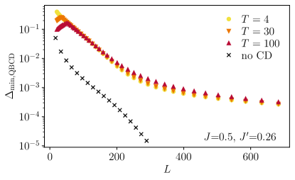
Figure 9: Gap amplification from the QBCD term, Eq. (36). Comparing with Fig. 5, one can see that $H^{\mathrm{QBCD}}$ is able to enlarge the minimal gap on the adiabatic path by a significant amount for all system sizes and driving times.

The QBCD Hamiltonian, Eq. (36), cancels exactly the transition between the ground and first excited states only at the gap-closing point; however, it also provides an efficient CD term in the neighborhood thereof. This feature can be inferred from the results shown in Fig. 9 and 10: both the gap $\Delta_{{\min},\mathrm{QBCD}}$ and the ground state fidelity are significantly increased with respect to the bare Hamiltonian. Here, the fidelity is captured by the kink number, since a value $K<1$ can come only from the ground state. In particular, one can see from Fig. 10a that for values of $T$ for which the bare Hamiltonian exhibits a kink number plateauing very close to 1, the QBCD term is able to lower it to $\expectationvalue{K}_{T}\approx 0.5$. This implies that the ground state is found at the end of the protocol with the finite probability of $\approx 0.5$, which is significantly larger than the one found with the bare protocol.

Figure 10: Performance of the driving assisted by the QBCD term, Eq. (36). The expectation value of the kink number on the final state plateaus for intermediate driving times, but the actual value of $\expectationvalue{K}_{T}$ is reduced when employing $H^{\mathrm{QBCD}}_{1}$ (dashed lines) with respect to the bare evolution (solid lines).

Finally, let us investigate the efficiency of the presented variational and QBCD approaches from the perspective of energy resources. While reducing external resources is essential for experimental realizations [110, 111], the energetic costs determine the speed at which the assisted process can stay adiabatic [50, 112, 113]. The Hilbert-Schmidt norm of the Hamiltonians, defined as $\|H_{1}\|^{2}=\mathrm{Tr}[H^{\dagger}_{1}\,H_{1}]$, provides a natural measure to quantify the cost of CD [50, 53, 60, 61]. It can be shown (see App. D) that the energy costs of the low-order expansions grow as

$$\left\|H_{1}^{(1,2)}\right\|^{2}\sim L$$ (37)

for the first- and second-order variational expansions, respectively. The QB approach surpasses the variational method in this aspect as well. As shown in App. D, the numerator and the denominator in Eq. (36) grow as (to leading order in $\ell$)

$$\Delta_{\min}\simeq\ell(\lambda-1)e^{-(\ell-1)\kappa}(1+e^{-2\mu})\\ +\ell\lambda\left(e^{-\ell\kappa-2\mu}+e^{-(\ell-2)\kappa}\right)$$ (38)

and

$$(\psi_{\mathrm{R}}|\partial_{\lambda}\mathcal{H}[\lambda_{c}]|\psi_{\mathrm{L}})\approx\\ \ell\left(e^{-(\ell-1)\kappa}(1+e^{-2\mu})+e^{-\ell\kappa-2\mu}+e^{-(\ell-2)\kappa}\right).$$ (39)

The two equations above imply a constant norm to leading order:

$$\left\|\mathcal{H}^{\mathrm{QBCD}}\right\|^{2}\sim O(1)\,.$$ (40)

This fact is a consequence of the exponentially localized nature of the two single-particle states involved in the avoided crossing and their appearance both in the gap and the transition matrix element.

To incorporate also the time dependence in the computation, in Fig. 11 the quantities $\frac{1}{T}\int_{0}^{T}\mathrm{d}t\,\|H_{1}\|^{2}$ are presented. It is clearly demonstrated that $\|H_{1}^{(1)}\|$ and $\|H_{1}^{(2)}\|$ increase with the system size, while $\|\mathcal{H}^{\mathrm{QBCD}}\|$ remains independent of $L$ to leading order. Thus, the QBCD approach not only achieves significantly larger fidelities to the target state, but it does so with a constant energy cost.

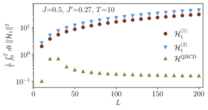
Figure 11: Energetic cost of implementing the counterdiabatic terms, as measured by the average Hilbert-Schmidt norm of the Hamiltonian along the driving path. While the first- and second-order variational terms have a cost that grows with the system size, the QBCD approach of Eq. (36) converges to an $L$-independent value.

VI Discussion

In this work, we investigated how the quantum adiabatic dynamics can be assisted in overcoming a spin-glass bottleneck with the use of counterdiabatic driving (CD). The model used is an Ising chain admitting a free-fermionic description, first introduced in Ref. [99], that displays both a gap exponentially small in the system size and two degenerate ground states that differ macroscopically from each other in terms of spin flips. The solvability of the model, however, was used only to reach larger system sizes and extract the asymptotic scalings: most of our analysis can be applied without substantial modifications to NP-hard Ising Hamiltonians. For this reason, we chose to employ CD terms that can be constructed efficiently on a classical computer: we resorted to two- and three-body ansatzes with coefficients fixed from the Floquet-Krylov variational principle [58, 59]. A key finding is that, while these CD ansatzes can amplify exponentially the size of the minimal gap along the adiabatic path, such gap remains exponentially small in the system size $L$, and the probability of ending up in the ground state at the end of the protocol is correspondingly very small for times shorter than $\sim e^{\alpha L}$, with $\alpha$ given in Eq. (19).

Our analysis highlights key features of CD of frustrated spin systems. First, from the gap characterization in Sec. IV.1, it can be inferred that CD is able to amplify the gap exponentially in the diabatic regime, and thus reduce substantially the diabatic transitions. However, reaching the regime of driving times where diabatic transitions come solely from the exponentially small ground state gap, the first two CD terms provide negligible improvement (see Figs. 7 and 8) and higher order expansions are required. On the other hand, slowing down the driving schedule also reduces the overall strength of the CD term, given the $\partial_{t}\lambda$ prefactor in Eq. (21). These features prevent the construction of an effective CD term bearing the adiabatic limit.

In addition, CD techniques, including the variational formulation [58, 59, 60], aim at keeping the evolving state as close as possible to the instantaneous ground state. The simplicity of the model allows us to identify a single transition from one end to the other of the effective chain, Eq. (16). Thus, in crossing the first-order phase transition, the state needs to be modified extensively in order to adjust to the change in the ground state.

These generic features highlight the efficiency and limitations of CD in its standard formulation. Approaches different from an a priori action minimization could be more effective in fighting bottlenecks. One option is to integrate the CD ansatzes with optimal control methods, as in QAOA [63, 62, 64, 65], where an iterative optimization of the control fields is performed using only the final state reached by the dynamics [77]. However, such numerical optimization allows for little analytical control and might be impeded by control landscape transitions [114, 115, 116, 117].

As a way out, we have introduced the QBCD Hamiltonian in Sec. V, which shares the structure of the Hamiltonian for the time-optimal evolution in the quantum brachistochrone problem for the associated subspace of localized edge states. With the help of the QBCD Hamiltonian, the success rate of the protocol increases from a vanishing probability to almost 0.5, as indicated by the average kink number at the end of the schedule. While it is a challenging task to implement non-local Hamiltonians with multi-body interactions in quantum devices, its realization is amenable to digital and digital-analog quantum simulation approaches. In addition, the QBCD Hamiltonian in Eq. (36) relies on the approximate spectral properties at a single value of the control parameter. This approach is remarkable in that its overall energy cost, as quantified by the Hilbert-Schmidt norm of the Hamiltonian, remains finite, as the multiple-body terms are exponentially suppressed. This particular combination of features hints at the fact that the hardness of crossing the exponentially small gaps is of entropic rather than energetic origin [118]: one does not need access to strong control fields but rather to some information regarding where to steer the quantum state. In this respect, an interesting prospect is to combine approximate CD and QBCD schemes with strategies such as reverse quantum annealing [104, 105, 106], the use of bias field [119, 87], Lyapunov control [67, 68], and the engineering of control terms with approximate knowledge of the critical point.

Appendix A Free-fermion representation of the Hamiltonian

A.1 Jordan-Wigner transformation and Dirac fermions

Start from the Hamiltonian (1). By applying a set of one-qubit gates

$$U=\frac{1}{\sqrt{2}}\begin{pmatrix}1&-1\\ 1&1\end{pmatrix},$$ (41)

by virtue of the identities

$$U\sigma^{x}U^{\dagger}=-\tilde{\sigma}^{z},\qquad U\sigma^{y}U^{\dagger}=\tilde{\sigma}^{y},\qquad U\sigma^{z}U^{\dagger}=\tilde{\sigma}^{x},$$ (42)

one can rewrite equivalently

$$H[\lambda]=\sum_{j=1}^{L}\left[-\lambda J_{j}\tilde{\sigma}^{x}_{j}\tilde{\sigma}^{x}_{j+1}+(1-\lambda)\tilde{\sigma}_{j}^{z}\right]$$ (43)

(tildes are used to distinguish the two sets of Pauli matrices for later convenience). This form of the Hamiltonian is convenient for a Jordan-Wigner transformation to be applied: one passes from spins $\{\tilde{\sigma}_{j}\}$ to Dirac fermions $\{c_{j}^{\phantom{\dagger}},c_{j}^{\dagger}\}$ by means of the identities

$$\tilde{\sigma}_{j}^{+}=e^{-i\pi\Sigma_{j}}c_{j}^{\dagger},\qquad\tilde{\sigma}_{j}^{-}=e^{i\pi\Sigma_{j}}c_{j},\qquad\tilde{\sigma}_{j}^{z}=2c_{j}^{\dagger}c_{j}^{\phantom{\dagger}}-1,$$ (44)

where the string operator $\Sigma_{j}$ in the exponent reads

$$\Sigma_{j}:=\sum_{k=1}^{j-1}c_{k}^{\dagger}c_{k}^{\phantom{\dagger}}.$$ (45)

Another possible way of writing the transformation is

$$c_{j}^{\dagger}=\prod_{k=1}^{j-1}\big{(}-\tilde{\sigma}_{k}^{z}\big{)}\,\tilde{\sigma}_{j}^{+},\qquad c_{j}=\prod_{k=1}^{j-1}\big{(}-\tilde{\sigma}_{k}^{z}\big{)}\,\tilde{\sigma}_{j}^{-}.$$ (46)

Then, the fermionic vacuum $\ket{0_{c}}$ corresponds to spins positively aligned along $x$-axis in the original basis ($\ket{0_{c}}=\ket{\rightarrow}$), and the fully occupied fermionic state corresponds to the spins anti-aligned along $x$-axis ($\ket{1_{c}}=\ket{\leftarrow}$).

Applying the Jordan-Wigner transformation to Eq. (43), one finds

$$H[\lambda] =\sum_{j=1}^{L}\left[-\lambda J_{j}\left(e^{-i\pi\Sigma_{j}}c_{j}^{\dagger}+e^{i\pi\Sigma_{j}}c_{j}\right)\left(e^{-i\pi\Sigma_{j+1}}c_{j+1}^{\dagger}+e^{i\pi\Sigma_{j+1}}c_{j+1}\right)+(1-\lambda)\left(2c_{j}^{\dagger}c_{j}^{\phantom{\dagger}}-1\right)\right]$$ (47)

$$=\sum_{j=1}^{L}\left[-\lambda J_{j}\left(c_{j}^{\dagger}e^{-i\pi c_{j}^{\dagger}c_{j}^{\phantom{\dagger}}}c_{j+1}^{\dagger}+c_{j}^{\dagger}e^{i\pi c_{j}^{\dagger}c_{j}^{\phantom{\dagger}}}c_{j+1}+c_{j}e^{-i\pi c_{j}^{\dagger}c_{j}^{\phantom{\dagger}}}c_{j+1}^{\dagger}+c_{j}e^{i\pi c_{j}^{\dagger}c_{j}^{\phantom{\dagger}}}c_{j+1}\right)+2(1-\lambda)c_{j}^{\dagger}c_{j}^{\phantom{\dagger}}\right]-(1-\lambda)L$$ (48)

$$=\sum_{j=1}^{L}\left[-\lambda J_{j}\left(c_{j}^{\dagger}c_{j+1}^{\dagger}+c_{j}^{\dagger}c_{j+1}^{\phantom{\dagger}}-c_{j}^{\phantom{\dagger}}c_{j+1}^{\dagger}-c_{j}c_{j+1}\right)+2(1-\lambda)c_{j}^{\dagger}c_{j}^{\phantom{\dagger}}\right]-(1-\lambda)L.$$ (49)

The Hamiltonian is manifestly a quadratic form in the creation/annihilation operators. In order to fix the boundary conditions, one needs to look back at the original Hamiltonian (1). In terms of the spins, the boundary conditions are periodic: $\sigma_{j+L}\equiv\sigma_{j}$. However, for the fermionic operators, it holds $c_{j+L}=+c_{j}$ or $c_{j+L}=-c_{j}$ depending on whether there is an odd or even number of fermions, respectively. Since the initial state (ground state at $\lambda=0$) is the fermionic vacuum $\ket{0_{c}}$, the correct sector to take is the even one.

In order to simplify things, we will not use the relation $c_{j+L}=-c_{j}$, but equivalently use $c_{j+L}=c_{j}$ and flip the sign the last coupling $J_{L}\to-J_{L}$, while still working within the even parity sector. In order to keep track of this change, we use tildes:

$$\tilde{J}_{j}:=\begin{cases}J_{j}&\text{if }j\neq L\\ -J_{L}&\text{if }j=L.\end{cases}$$ (50)

Therefore, the Hamiltonian reads

$$H[\lambda] =\sum_{j=1}^{L}\left[-\lambda\tilde{J}_{j}\left(c_{j}^{\dagger}c_{j+1}^{\dagger}+c_{j}^{\dagger}c_{j+1}^{\phantom{\dagger}}-c_{j}^{\phantom{\dagger}}c_{j+1}^{\dagger}-c_{j}c_{j+1}\right)+2(1-\lambda)c_{j}^{\dagger}c_{j}^{\phantom{\dagger}}\right]-(1-\lambda)L$$ (51)

$$=\sum_{j=1}^{L}\left[-\lambda\tilde{J}_{j}\left(c_{j}^{\dagger}-c_{j}^{\phantom{\dagger}}\right)\left(c_{j+1}^{\dagger}+c_{j+1}^{\phantom{\dagger}}\right)+2(1-\lambda)c_{j}^{\dagger}c_{j}^{\phantom{\dagger}}\right]-(1-\lambda)L.$$ (52)

Notice that if any operator (different from the Hamiltonian) has terms coupling $c_{L}$ with $c_{L+1}$, also there the sign must be flipped. We will use tildes to remember this fact.

A.2 Majorana fermions

From the Dirac fermion representation $\{c_{i}^{\phantom{\dagger}},c_{j}^{\dagger}\}_{j=1}^{L}$, one can pass to an equivalent Majorana fermionic representation $\{\gamma_{2j-1},\gamma_{2j}\}_{j=1}^{L}$ by effectively doubling the length of the chain. The defining relations are

$$\gamma_{2j-1}:=\frac{1}{\sqrt{2}}\left(c_{j}^{\phantom{\dagger}}+c_{j}^{\dagger}\right),\qquad\gamma_{2j}:=\frac{i}{\sqrt{2}}\left(c_{j}^{\phantom{\dagger}}-c_{j}^{\dagger}\right),$$ (53)

and the inverse transformation is

$$c_{j}^{\dagger}=\frac{\gamma_{2j-1}+i\gamma_{2j}}{\sqrt{2}},\qquad c_{j}^{\phantom{\dagger}}=\frac{\gamma_{2j-1}-i\gamma_{2j}}{\sqrt{2}},$$ (54)

leading to anticommutation relations

$$\left\{\gamma_{k},\gamma_{k^{\prime}}\right\}=\delta_{k,k^{\prime}}.$$ (55)

One can rewrite

$$H[\lambda]=-2i\sum_{j=1}^{L}\big{[}\lambda\tilde{J}_{j}\gamma_{2j}\gamma_{2j+1}+(1-\lambda)\gamma_{2j-1}\gamma_{2j}\big{]}.$$ (56)

The boundary conditions inherited by the Dirac fermions entail $\gamma_{k+2L}=-\gamma_{k}$ (even parity sector) but, as stated above, we are employing $\gamma_{k+2L}=\gamma_{k}$ and the flipped couplings $\tilde{J}_{j}$.

A.3 Reflection parity symmetry

The Hamiltonian (1), and thus its Majorana representation (56), is odd under the chiral reflection parity symmetry $\widetilde{\Pi}_{\mathrm{R}}$ defined by Eq. (10), i.e. $\widetilde{\Pi}_{\mathrm{R}}\gamma_{k}\widetilde{\Pi}_{\mathrm{R}}=\gamma_{2L-k+1}$. Indeed, the couplings satisfy $J_{j}=J_{L-j}$, and one can write

$$\widetilde{\Pi}_{\mathrm{R}}H\widetilde{\Pi}_{\mathrm{R}} =-2i\sum_{j=1}^{L}\big{[}\lambda\tilde{J}_{j}\gamma_{2L-2j+1}\gamma_{2L-2j}+(1-\lambda)\gamma_{2L-2j+2}\gamma_{2L-2j+1}\big{]}$$ (57)

$$=-2i\sum_{j=1}^{L}\big{[}\lambda\tilde{J}_{L-j}\gamma_{2L-2j+1}\gamma_{2L-2j}+(1-\lambda)\gamma_{2L-2j+2}\gamma_{2L-2j+1}\big{]}$$ (58)

$$=-2i\sum_{l=0}^{L-1}\big{[}\lambda\tilde{J}_{l}\gamma_{2l+1}\gamma_{2l}+(1-\lambda)\gamma_{2l+2}\gamma_{2l+1}\big{]}=-H.$$ (59)

In the first line, the operator $\widetilde{\Pi}_{\mathrm{R}}$ was applied on the $\gamma$’s; in the second line, $\tilde{J}_{j}$ was exchanged with $\tilde{J}_{L-j}$; in the third line, it was set $l:=L-j$. $H$ is odd under the reflection parity $\widetilde{\Pi}_{\mathrm{R}}$, thus $\widetilde{\Pi}_{\mathrm{R}}$ is a chiral symmetry for $H$ [100].

Before moving on, it is interesting to express the chiral reflection parity symmetry also in terms of the Dirac operators:

$$\widetilde{\Pi}_{\mathrm{R}}c_{j}\widetilde{\Pi}_{\mathrm{R}} =\widetilde{\Pi}_{\mathrm{R}}\frac{\gamma_{2j-1}-i\gamma_{2j}}{\sqrt{2}}\widetilde{\Pi}_{\mathrm{R}}=\frac{\gamma_{2L-2j+2}-i\gamma_{2L-2j+1}}{\sqrt{2}}=-ic^{\dagger}_{L-j+1},$$ (60a)

$$\widetilde{\Pi}_{\mathrm{R}}c_{j}^{\dagger}\widetilde{\Pi}_{\mathrm{R}} =\widetilde{\Pi}_{\mathrm{R}}\frac{\gamma_{2j-1}+i\gamma_{2j}}{\sqrt{2}}\widetilde{\Pi}_{\mathrm{R}}=\frac{\gamma_{2L-2j+2}+i\gamma_{2L-2j+1}}{\sqrt{2}}=ic_{L-j+1},$$ (60b)

which shows that $\widetilde{\Pi}_{\mathrm{R}}$ also exchanges particles and holes. In terms of the spin operators, it holds instead

$$\widetilde{\Pi}_{\mathrm{R}}\sigma_{j}^{x}\widetilde{\Pi}_{\mathrm{R}}=-\widetilde{\Pi}_{\mathrm{R}}\tilde{\sigma}_{j}^{z}\widetilde{\Pi}_{\mathrm{R}}=-\widetilde{\Pi}_{\mathrm{R}}c_{j}^{\dagger}c_{j}^{\phantom{\dagger}}\widetilde{\Pi}_{\mathrm{R}}=-ic_{L-j+1}(-i)c_{L-j+1}^{\dagger}=c_{L-j+1}^{\dagger}c_{L-j+1}=\tilde{\sigma}_{L-j+1}^{z}=-\sigma_{L-j+1}^{x},$$ (61)

while $\widetilde{\Pi}_{\mathrm{R}}\sigma_{j}^{z}\widetilde{\Pi}_{\mathrm{R}}$ involves also the transformation of the Jordan-Wigner string. Thus, the chiral reflection parity symmetry is non-local in the spin representation of the Hamiltonian.

The non-locality of $\widetilde{\Pi}_{\mathrm{R}}$ in the spin representation is “dual” to the non-locality of $\Pi_{\mathrm{R}}$ in the fermionic representation. Indeed, the presence of the Jordan-Wigner string entails the transformation rules

$$\Pi_{\mathrm{R}}c_{j}\Pi_{\mathrm{R}} =\Pi_{\mathrm{R}}\prod_{k=1}^{j-1}\big{(}-\sigma_{k}^{z}\big{)}\sigma_{j}^{-}\Pi_{\mathrm{R}}=\prod_{k=1}^{j-1}\big{(}-\sigma_{L-k+1}^{z}\big{)}\sigma_{L-j+1}^{-}=(-1)^{N_{\mathrm{F}}}\prod_{k=1}^{L-j+1}\big{(}-\sigma_{k}^{z}\big{)}\sigma_{L-j+1}^{-}$$

$$=(-1)^{N_{\mathrm{F}}}\left(1-2c_{L-j+1}^{\dagger}c_{L-j+1}^{\phantom{\dagger}}\right)c_{L-j+1}=(-1)^{N_{\mathrm{F}}}c_{L-j+1},$$ (62a)

$$\Pi_{\mathrm{R}}c_{j}^{\dagger}\Pi_{\mathrm{R}} =\Pi_{\mathrm{R}}\prod_{k=1}^{j-1}\big{(}-\sigma_{k}^{z}\big{)}\sigma_{j}^{+}\Pi_{\mathrm{R}}=\prod_{k=1}^{j-1}\big{(}-\sigma_{L-k+1}^{z}\big{)}\sigma_{L-j+1}^{+}=(-1)^{N_{\mathrm{F}}}\prod_{k=1}^{L-j+1}\big{(}-\sigma_{k}^{z}\big{)}\sigma_{L-j+1}^{+}$$

$$=(-1)^{N_{\mathrm{F}}}\left(1-2c_{L-j+1}^{\dagger}c_{L-j+1}^{\phantom{\dagger}}\right)c_{L-j+1}^{\dagger}=-(-1)^{N_{\mathrm{F}}}c_{L-j+1}^{\dagger},$$ (62b)

where $N_{\mathrm{F}}:=\sum_{j=1}^{L}c_{j}^{\dagger}c_{j}^{\phantom{\dagger}}$ is the total fermion number operator. The prefactor $(-1)^{N_{\mathrm{F}}}$ is a non-local operator that makes it more difficult to define creation and annihilation operators symmetrized with respect to $\Pi_{\mathrm{R}}$. This is the reason why it is convenient to use the chiral symmetry $\widetilde{\Pi}_{\mathrm{R}}$ instead of the unitary symmetry $\Pi_{\mathrm{R}}$ when working with the Dirac fermions. A similar situation takes place in the Majorana representation. A comprehensive, modern view on the subtleties of symmetries in Ising-like chains can be found in Ref. [120].

A.4 Reflection-symmetrized representation

Let us introduce symmetrized operators, as in Eqs. (12) in the main text. The inverse transformation is

$$\gamma_{k} =\frac{\Gamma_{k}^{+}-\Gamma_{k}^{-}}{\sqrt{2}i},\qquad k=1,3,\dots,L,$$ (63a)

$$\gamma_{k} =\frac{\Gamma_{k}^{+}+\Gamma_{k}^{-}}{\sqrt{2}},\qquad k=2,4,\dots,L-1,$$ (63b)

$$\gamma_{k} =\frac{\Gamma_{2L-k+1}^{+}+\Gamma_{2L-k+1}^{-}}{\sqrt{2}},\qquad k=L+1,L+3,\dots,2L,$$ (63c)

$$\gamma_{k} =\frac{\Gamma_{2L-k+1}^{+}-\Gamma_{2L-k+1}^{-}}{\sqrt{2}i},\qquad k=L+2,L+3,\dots,2L-1.$$ (63d)

Let us split the Hamiltonian (56) into the different contributions: for $-\lambda J$ or $(1-\lambda)$, and bulk or boundary. It holds for $j=1,2,\dots,\ell$

$$\tilde{J}_{j}\gamma_{2j}\gamma_{2j+1}+\tilde{J}_{L-j}\gamma_{2L-2j}\gamma_{2L-2j+1} =\tilde{J}_{j}\left[\frac{\Gamma_{2j}^{+}+\Gamma_{2j}^{-}}{\sqrt{2}}\frac{\Gamma_{2j+1}^{+}-\Gamma_{2j+1}^{-}}{\sqrt{2}i}+\frac{\Gamma_{2j+1}^{+}+\Gamma_{2j+1}^{-}}{\sqrt{2}}\frac{\Gamma_{2j}^{+}-\Gamma_{2j}^{-}}{\sqrt{2}i}\right]$$

$$=-\frac{i\tilde{J}_{j}}{2}\left[\left(\Gamma_{2j}^{+}+\Gamma_{2j}^{-}\right)\left(\Gamma_{2j+1}^{+}-\Gamma_{2j+1}^{-}\right)-\left(\Gamma_{2j}^{+}-\Gamma_{2j}^{-}\right)\left(\Gamma_{2j+1}^{+}+\Gamma_{2j+1}^{-}\right)\right]$$

$$=i\tilde{J}_{j}\left(\Gamma_{2j}^{+}\Gamma_{2j+1}^{-}-\Gamma_{2j}^{-}\Gamma_{2j+1}^{+}\right),$$ (64)

and

$$(1-\lambda)(\gamma_{2j-1}\gamma_{2j}+\gamma_{2L-2j-1}\gamma_{2L-2j}) =(1-\lambda)\left[\frac{\Gamma_{2j-1}^{+}-\Gamma_{2j-1}^{-}}{\sqrt{2}i}\frac{\Gamma_{2j}^{+}+\Gamma_{2j}^{-}}{\sqrt{2}}+\frac{\Gamma_{2j}^{+}-\Gamma_{2j}^{-}}{\sqrt{2}i}\frac{\Gamma_{2j-1}^{+}+\Gamma_{2j-1}^{-}}{\sqrt{2}}\right]$$

$$=-\frac{i(1-\lambda)}{2}\left[\left(\Gamma_{2j-1}^{+}-\Gamma_{2j-1}^{-}\right)\left(\Gamma_{2j}^{+}+\Gamma_{2j}^{-}\right)-\left(\Gamma_{2j-1}^{+}+\Gamma_{2j-1}^{-}\right)\left(\Gamma_{2j}^{+}-\Gamma_{2j}^{-}\right)\right]$$

$$=i(1-\lambda)\left(\Gamma_{2j-1}^{-}\Gamma_{2j}^{+}-\Gamma_{2j-1}^{+}\Gamma_{2j}^{-}\right),$$ (65)

while for the other sites

$$\tilde{J}_{L}\gamma_{2L}\gamma_{1}=\tilde{J}_{L}\frac{\Gamma_{1}^{+}+\Gamma_{1}^{-}}{\sqrt{2}}\frac{\Gamma_{1}^{+}-\Gamma_{1}^{-}}{\sqrt{2}i}=\frac{i\tilde{J}_{L}}{2}\left(\Gamma_{1}^{+}\Gamma_{1}^{-}-\Gamma_{1}^{-}\Gamma_{1}^{+}\right),$$ (66)

$$(1-\lambda)\gamma_{L}\gamma_{L+1}=(1-\lambda)\frac{\Gamma_{L}^{+}-\Gamma_{L}^{-}}{\sqrt{2}i}\frac{\Gamma_{L}^{+}+\Gamma_{L}^{-}}{\sqrt{2}}=\frac{i}{2}(1-\lambda)\left(\Gamma_{L}^{-}\Gamma_{L}^{+}-\Gamma_{L}^{+}\Gamma_{L}^{-}\right).$$ (67)

The Hamiltonian acquires the form

$$H[\lambda]=2\lambda\sum_{j=1}^{\ell}\tilde{J}_{j}\left(\Gamma_{2j}^{+}\Gamma_{2j+1}^{-}-\Gamma_{2j}^{-}\Gamma_{2j+1}^{+}\right)+2(1-\lambda)\sum_{j=1}^{\ell}\left(\Gamma_{2j-1}^{-}\Gamma_{2j}^{+}-\Gamma_{2j-1}^{+}\Gamma_{2j}^{-}\right)\\ +\lambda\tilde{J}_{L}\left(\Gamma_{1}^{+}\Gamma_{1}^{-}-\Gamma_{1}^{-}\Gamma_{1}^{+}\right)+(1-\lambda)\left(\Gamma_{L}^{-}\Gamma_{L}^{+}-\Gamma_{L}^{+}\Gamma_{L}^{-}\right),$$ (68)

which is the same of Eq. (14) in the main text.

A.5 Transformation of states

From the equations above, one can also find the relation between the vacuum state for the $c$’s and the one for the $\Gamma$’s. Defining $\ket{0_{c}}$ to be the state annihilated by all $c_{j}$’s, and $\ket{0_{\Gamma}}$ to be the one annihilated by all the $\Gamma_{k}^{-}$’s, it holds

$$\ket{0_{c}}=\prod_{k=1}^{\ell}\left(1+\Gamma_{2k-1}^{+}\Gamma_{2k}^{+}\right)\ket{0_{\Gamma}},$$ (69)

as one can check by directly applying each $c_{j}$ expressed in terms of the $\Gamma_{k}^{\pm}$’s.

Appendix B Diagonalization of the effective hopping model

The purpose of this Appendix is to provide the eigendecomposition of the system Hamiltonian (1) by diagonalizing the effective 1D hopping model Eq. (16). It is convenient to rewrite the matrix as

$$\mathcal{H}=\lambda\begin{pmatrix}-J_{L}&-B&&&&&\\ -B&0&J_{1}&&&&\\ &J_{1}&0&-B&&&\\ &&-B&0&J_{2}&&\\ &&&J_{2}&\ddots&\ddots&\\ &&&&\ddots&0&J_{\ell}\\ &&&&&J_{\ell}&-B\end{pmatrix},$$ (70)

where $B:=(1-\lambda)/\lambda$.

As a first thing, notice that for the choice of $J_{j}$’s in Eq. (2), the model is translation invariant in bulk (step 2), while only the sites $1$, $L-1$ and $L$ experience different couplings. This fact suggests that plane waves are eigenfunctions of the system, provided the boundary conditions are fixed.

Second, notice that for $B=0$ (i.e., at the end of the anneal), there is an eigenstate localized at the left end $j=0$, namely $(1\ 0\ 0\dots)^{T}$. Similarly, when $B=\infty$ (i.e.,  at the beginning of the anneal), one eigenstate is localized at the right end, namely $(0\dots 0\ 1)^{T}$. In the following, these localized states are determined with a scattering approach.

B.1 Plane waves in the bulk

Let us start by constructing the plane wave eigenvectors of Eq. (70) in the bulk. The eigenvalue equation $\mathcal{H}|\psi)=\lambda\epsilon|\psi)$ reads, in components,

$$\begin{cases}-B\psi_{2j}+\psi_{2j-2}=\epsilon\psi_{2j-1}\\ \psi_{2j+1}-B\psi_{2j-1}=\epsilon\psi_{2j},\end{cases}$$ (71)

where the couplings $J_{j}$ of Eq. (2) have been specified. Using the Fourier ansatz

$$\begin{pmatrix}\psi_{2j-1}\\ \psi_{2j}\end{pmatrix}\sim e^{ikj}\begin{pmatrix}a_{k}\\ b_{k}\end{pmatrix},$$ (72)

the bulk eigenvalue equation acquires the form

$$\begin{cases}-Bb_{k}+e^{-ik}b_{k}=\epsilon_{k}a_{k}\\ e^{ik}a_{k}-Ba_{k}=\epsilon_{k}b_{k}.\end{cases}$$ (73)

From the linear system above, one determines

$$(e^{-ik}-B)(e^{ik}-B)=\epsilon^{2}_{k}$$ (74)

and

$$\frac{a_{k}}{b_{k}}=\frac{\epsilon_{k}}{e^{ik}-B}.$$ (75)

The first equation fixes the dispersion relation in the bulk, and the second the relative scale of $a_{k}$ to $b_{k}$. They need to be supplemented by the boundary conditions, which fix the admissible values of $k$, and the normalization condition, which fixes the overall scale of the eigenvector. In order to simplify things, it is instrumental to work already in the thermodynamic limit $L\to\infty$, since this way, the left and right boundary conditions are completely decoupled. The two will be considered separately in the following subsections.

B.2 Left-localized state

Here, consider a semi-infinite chain starting from $j=0$ and ending at $j=+\infty$. The only boundary condition one needs to take into account is provided by the eigenvalue equation at the first site:

$$J^{\prime}\psi_{1}-B\psi_{2}=\epsilon\psi_{1},$$ (76)

that can be rewritten as

$$J^{\prime}a_{k}-Bb_{k}=\epsilon_{k}a_{k}\qquad\implies\qquad\frac{a_{k}}{b_{k}}=\frac{B}{J^{\prime}-\epsilon_{k}}.$$ (77)

When supplemented with Eqs. (74), (75) and the normalization condition, one obtains four equations for the four unknowns $a_{k}$,$b_{k}$,$k$,$\epsilon_{k}$. Here, we consider only the localized edge state, for which $k\equiv i\kappa$, $\kappa>0$. Eliminating $a_{k}/b_{k}$ and $\epsilon_{k}$ from Eq. (77) via Eqs. (74) and (75), one finds

$$\frac{1-e^{\kappa}B}{1-e^{-\kappa}B}=(J^{\prime})^{2},$$ (78)

which has a real positive solution

$$\kappa=\ln\frac{1-(J^{\prime})^{2}+\sqrt{4B^{2}(J^{\prime})^{2}+[(J^{\prime})^{2}-1]^{2}}}{2B}.$$ (79)

B.3 Right-localized state

Here, consider the half-infinite chain that starts at $j=-\infty$ and ends at $j=L$. Besides Eqs. (74) and (75) that describe the wave propagation in the bulk, the two boundary conditions at the right end read

$$-B\psi_{L-2}+J_{\ell}\psi_{L}=\epsilon\psi_{L-1},\qquad J_{\ell}\psi_{L-1}-B\psi_{L}=\epsilon\psi_{L}.$$ (80)

Being the last site odd, the Fourier ansatz Eq. (72) needs to be supplemented by

$$\psi_{L}\sim e^{ikL}c_{k}.$$ (81)

The boundary conditions Eq. (80) read, in terms of the Fourier ansatz,

$$-Ba_{k}+Je^{ik}c_{k}=\epsilon_{k}b_{k},\qquad Jb_{k}e^{-ik}-Bc_{k}=\epsilon_{k}c_{k}.$$ (82)

From here, one can eliminate $c_{k}$, obtaining

$$\epsilon_{k}b_{k}+Ba_{k}=\frac{J^{2}b_{k}}{\epsilon_{k}+B}.$$ (83)

Now, Eqs. (74), (75), (83) and the normalization condition are again four equations for the four unknowns $a_{k}$,$b_{k}$,$k$,$\epsilon_{k}$. The right-localized state will have an imaginary momentum $k\equiv-i\kappa$, $\kappa>0$, that can be determined by combining the cited equations. Since this would lead to cumbersome equations, it is convenient to utilize a workaround to determine the avoided crossing directly, as in Ref. [99].

B.4 Avoided crossing

The avoided crossing takes place at the value of $B$ such that $\epsilon_{k}$ is the same for the left ($\mathrm{L}$) and right ($\mathrm{R}$) localized states. In principle, one should impose $(\epsilon_{k})_{\mathrm{L}}\equiv(\epsilon_{k})_{\mathrm{R}}$ by using the expression (74) with the values of $\kappa_{\mathrm{L}}$ and $\kappa_{\mathrm{R}}$ determined above. However, it is convenient to notice that, because of Eq. (74), it must hold $\kappa_{\mathrm{L}}=\kappa_{\mathrm{R}}$, and from Eq. (75) follows $(a_{k}/b_{k})_{\mathrm{L}}=(b_{k}/a_{k})_{\mathrm{R}}$ (being $k_{\mathrm{R}}=-k_{\mathrm{L}}$ for the choice of $i$’s). Thus, one determines $(a_{k}/b_{k})_{\mathrm{L}}$ from Eq. (77), and equates it to $(b_{k}/a_{k})_{\mathrm{R}}$ from Eq. (83), finding

$$\epsilon+B=\frac{J^{2}}{J^{\prime}}.$$ (84)

Plugging above $\epsilon$ from Eq. (74), with $\kappa$ taken from Eq. (79), one determines the value of $B$ at which the crossing takes place:

$$B_{\mathrm{c}}=\frac{(1-J^{2})[J^{2}-(J^{\prime})^{2}]}{J^{\prime}[1-2J^{2}+(J^{\prime})^{2}]}.$$ (85)

From Eq. (84) follows

$$\epsilon_{\mathrm{c}}=\frac{(J^{\prime})^{2}-J^{4}}{J^{\prime}[1-2J^{2}+(J^{\prime})^{2}]},$$ (86)

and in turn from Eq. (74)

$$\kappa_{\mathrm{c}}=\ln\frac{J^{\prime}(1-J^{2})}{J^{2}-(J^{\prime})^{2}}.$$ (87)

From the equation above, the condition $\kappa>0$ implies for the couplings

$$J^{2}<J^{\prime},$$ (88)

which explains the requirement stated in Eq. (3).

The last step consists in determining the magnitude of the gap at the avoided level crossing. Since $|\psi_{\mathrm{L}})$ and $|\psi_{\mathrm{R}})$ determined above are not eigenfunctions of the chain of finite length, one can argue that

$$\Delta_{\min}\simeq(\psi_{\mathrm{L}}|\mathcal{H}|\psi_{\mathrm{R}})\sim\sum_{j=1}^{L}e^{-\kappa_{c}j/2}e^{-\kappa_{c}(L-j)/2}\sim e^{-\kappa_{c}L/2},$$ (89)

which corresponds to Eq. (19) in the main text. Indeed, the hybridization of $|\psi_{\mathrm{L}})$ and $|\psi_{\mathrm{R}})$ is approximately given by the off-diagonal matrix element $(\psi_{\mathrm{L}}|\mathcal{H}|\psi_{\mathrm{R}})$ in the reduced 2$\times$2 subspace spanned by $|\psi_{\mathrm{L}})$ and $|\psi_{\mathrm{R}})$ themselves. All the factors dropped in Eq. (89) are subleading with respect to the exponential term.

Appendix C Free-fermion representation of the counterdiabatic Hamiltonian

C.1 Chiral reflection parity of the CD Hamiltonian

As a first thing, let us investigate how the reflection parity symmetry acts on the CD Hamiltonian, Eq. (24). Using the fact that $\widetilde{\Pi}_{\mathrm{R}}H\widetilde{\Pi}_{\mathrm{R}}=-H$, as proven in Sec. A.3, it follows

$$\widetilde{\Pi}_{\mathrm{R}}H_{1}\widetilde{\Pi}_{\mathrm{R}} =-\frac{1}{2}\int_{-\infty}^{+\infty}dx\,f(x)\,\widetilde{\Pi}_{\mathrm{R}}e^{ixH}\partial_{\lambda}He^{-ixH}\widetilde{\Pi}_{\mathrm{R}}$$ (90)

$$=\frac{1}{2}\int_{-\infty}^{+\infty}dx\,f(x)\,e^{-ixH}\partial_{\lambda}He^{ixH}$$ (91)

$$=-\frac{1}{2}\int_{-\infty}^{+\infty}dy\,f(y)\,e^{iyH}\partial_{\lambda}He^{-iyH}=+H_{1},$$ (92)

having set $y:=-x$. Thus, $H_{1}$ is even under the chiral reflection parity, Eq. (10), while $H$ is odd. The same conclusion can be reached by noticing that in Eq. (25), there is an even number of $H$’s at every order of the expansion.

At the same time, $H_{1}$ is even under the standard reflection parity, Eq. (5), as can be checked directly from the spin representation.

C.2 First order ansatz

Let us move to the Hamiltonian (28). By applying the set of one-qubit gates defined in Eq. (41), one can rewrite

$$H_{1}^{(1)}[\lambda] =\sum_{j=1}^{L}\alpha_{j}\left(\tilde{\sigma}_{j}^{y}\tilde{\sigma}_{j+1}^{x}+\tilde{\sigma}_{j}^{x}\tilde{\sigma}_{j+1}^{y}\right)$$ (93)

$$=2i\sum_{j=1}^{L}\alpha_{j}\left(\tilde{\sigma}_{j}^{-}\tilde{\sigma}_{j+1}^{-}-\tilde{\sigma}_{j}^{+}\tilde{\sigma}_{j+1}^{+}\right).$$ (94)

This form of the CD Hamiltonian is expressed in terms of Dirac fermions, Eq. (44), as

$$H_{1}^{(1)}[\lambda] =-2i\sum_{j=1}^{L}\tilde{\alpha}_{j}\left(e^{-i\pi\Sigma_{j}}c_{j}^{\dagger}e^{-i\pi\Sigma_{j+1}}c_{j+1}^{\dagger}\right)+\mathrm{h.c.}$$ (95)

$$=-2i\sum_{j=1}^{L}\tilde{\alpha}_{j}\left(c_{j}^{\dagger}e^{-i\pi c^{\dagger}_{j}c^{\phantom{\dagger}}_{j}}c_{j+1}^{\dagger}\right)+\mathrm{h.c.}$$ (96)

$$=-2i\sum_{j=1}^{L}\tilde{\alpha}_{j}\left[c^{\dagger}_{j}c^{\dagger}_{j+1}+c_{j}c_{j+1}\right],$$ (97)

where there is a tilde on the $\alpha_{j}$’s because of the fermion parity symmetry, see above Eq. (50).

Next, one has to rewrite the Hamiltonian above in terms of Majorana fermions, Eq. (54):

$$H_{1}^{(1)}[\lambda] =-2i\sum_{j=1}^{L}\tilde{\alpha}_{j}\left[\frac{1}{2}(\gamma_{2j-1}+i\gamma_{2j})(\gamma_{2j+1}+i\gamma_{2j+2})+\frac{1}{2}(\gamma_{2j-1}-i\gamma_{2j})(\gamma_{2j+1}-i\gamma_{2j+2})\right]$$ (98)

$$=2i\sum_{j=1}^{L}\tilde{\alpha}_{j}\left[\gamma_{2j}\gamma_{2j+2}-\gamma_{2j-1}\gamma_{2j+1}\right].$$ (99)

It is convenient to check the reflection parity of the expression above for $H_{1}$:

$$\widetilde{\Pi}_{\mathrm{R}}H_{1}^{(1)}[\lambda]\widetilde{\Pi}_{\mathrm{R}} =2i\sum_{j=1}^{L}\tilde{\alpha}_{j}\left[\gamma_{2L-2j+1}\gamma_{2L-2j-1}-\gamma_{2L-2j+2}\gamma_{2L-2j}\right]$$ (100)

$$=2i\sum_{j=1}^{L}\tilde{\alpha}_{L-j}\left[\gamma_{2j+1}\gamma_{2j-1}-\gamma_{2j+2}\gamma_{2j}\right]$$ (101)

$$=2i\sum_{j=1}^{L}\tilde{\alpha}_{L-j}\left[\gamma_{2j}\gamma_{2j+2}-\gamma_{2j-1}\gamma_{2j+1}\right],$$ (102)

where in the first line Eq. (10) was used, and in the second it was changed $j\to L-j$. In order to have $\widetilde{\Pi}_{\mathrm{R}}H_{1}\widetilde{\Pi}_{\mathrm{R}}=H_{1}$, it must hold $\alpha_{j}\equiv\alpha_{L-j}$, which indeed follows from the variational equations (29).

At this point, one can pass to the symmetrized operators $\Gamma^{\pm}$. Using

$$-\tilde{\alpha}_{j}\gamma_{2j-1}\gamma_{2j+1}+\tilde{\alpha}_{L-j}\gamma_{2L-2j}\gamma_{2L-2j+2} =-\tilde{\alpha}_{j}\left(\Gamma_{2j-1}^{-}\Gamma_{2j+1}^{+}+\Gamma_{2j-1}^{+}\Gamma_{2j+1}^{-}\right),\qquad j=1,2,\dots,\ell,$$ (103a)

$$\tilde{\alpha}_{j}\gamma_{2j}\gamma_{2j+2}-\tilde{\alpha}_{L-j}\gamma_{2L-2j-1}\gamma_{2L-2j+1} =\tilde{\alpha}_{j}\left(\Gamma_{2j}^{+}\Gamma_{2j+2}^{-}+\Gamma_{2j}^{-}\Gamma_{2j+2}^{+}\right), j=1,2,\dots,\ell-1,$$ (103b)

$$\tilde{\alpha}_{\ell}\gamma_{2\ell}\gamma_{2\ell+2}-\tilde{\alpha}_{\ell+1}\gamma_{2\ell+1}\gamma_{2\ell+3} =\tilde{\alpha}_{\ell}\left(\Gamma_{2\ell}^{-}\Gamma_{2\ell+1}^{+}+\Gamma_{2\ell}^{+}\Gamma_{2\ell+1}^{-}\right),$$ (103c)

$$\tilde{\alpha}_{L}\left(-\gamma_{2L-1}\gamma_{1}+\gamma_{2L}\gamma_{2}\right) =\tilde{\alpha}_{L}\left(\Gamma_{1}^{+}\Gamma_{2}^{-}+\Gamma_{1}^{-}\Gamma_{2}^{+}\right),$$ (103d)

it follows

$$H_{1}^{(1)}[\lambda]=2i\sum_{j=1}^{\ell}\tilde{\alpha}_{j}\left(\Gamma_{2j+1}^{+}\Gamma_{2j-1}^{-}-\Gamma_{2j-1}^{+}\Gamma_{2j+1}^{-}\right)+2i\sum_{j=1}^{\ell-1}\tilde{\alpha}_{j}\left(\Gamma_{2j}^{+}\Gamma_{2j+2}^{-}-\Gamma_{2j+2}^{+}\Gamma_{2j}^{-}\right)\\ +2i\tilde{\alpha}_{\ell}\left(\Gamma_{2\ell}^{+}\Gamma_{2\ell+1}^{-}-\Gamma_{2\ell+1}^{+}\Gamma_{2\ell}^{-}\right)+2i\tilde{\alpha}_{L}\left(\Gamma_{1}^{+}\Gamma_{2}^{-}-\Gamma_{2}^{+}\Gamma_{1}^{-}\right).$$ (104)

The matrix representation reads (for $\ell=3$, thus $L=7$)

$$H_{1}^{(1)}[\lambda]=2\,\vec{\Gamma}^{+}\begin{pmatrix}0&-i\alpha_{7}&-i\alpha_{1}&&&&\\ i\alpha_{7}&0&0&i\alpha_{1}&&&\\ i\alpha_{1}&0&0&0&-i\alpha_{2}&&\\ &-i\alpha_{1}&0&0&0&i\alpha_{2}&\\ &&i\alpha_{2}&0&0&0&-i\alpha_{3}\\ &&&-i\alpha_{2}&0&0&i\alpha_{3}\\ &&&&i\alpha_{3}&-i\alpha_{3}&0\\ \end{pmatrix}\vec{\Gamma}^{-}.$$ (105)

C.3 Second order ansatz

When considered together the first and second-order approximate CD Hamiltonians $H_{1}^{(1)}+H_{1}^{(2)}$, one can check that the variational equations, obtained from the minimization of the action Eq. (26), are

$$\left[8(1-\lambda)^{2}+\lambda^{2}\left(J_{j-1}^{2}+2J_{j}^{2}+J_{j+1}^{2}\right)\right]\alpha_{j}+2\lambda^{2}J_{j}\left(J_{j-1}\alpha_{j-1}+J_{j+1}\alpha_{j+1}\right)+4\lambda(\lambda-1)(\beta_{j-1}J_{j-1}+\beta_{j}J_{j+1})=-J_{j},$$

$$\left[8(1-\lambda)^{2}+\lambda^{2}\left(J_{j-1}^{2}+J_{j}^{2}+J_{j+1}^{2}+J_{j+2}^{2}\right)\right]\beta_{j}+2\lambda^{2}\left(J_{j-1}J_{j+1}\beta_{j-1}+J_{j}J_{j+2}\beta_{j+1}\right)+4\lambda(\lambda-1)(\alpha_{j+1}J_{j}+\alpha_{j}J_{j+1})=0,$$ (106)

Thanks to the relation $J_{j}=J_{L-j}$, these equations are symmetric under the exchange

$$\alpha_{j} \longleftrightarrow\, \alpha_{L-j},\qquad j=1,2,\dots,L$$

$$\beta_{j} \longleftrightarrow \beta_{L-j-1},\qquad j=1,2,\dots,L-2$$ (107)

$$\beta_{L-1} \longleftrightarrow \beta_{L}.\qquad$$

One can check that the second order ansatz for the CD Hamiltonian, Eq. (30), is expressed in terms of Dirac fermions as

$$H_{1}^{(2)}[\lambda]=-2i\sum_{j=1}^{L}\tilde{\beta}_{j}\left[c^{\dagger}_{j}c^{\dagger}_{j+2}+c_{j}c_{j+2}\right].$$ (108)

Indeed, the same computation of App. C.2 applies, and the intermediate operator $\sigma_{j+1}^{x}$ just cancels the Jordan-Wigner string. The tilde on the $\beta_{j}$’s is again to remind that the sign in front of any operator that connects the last sites of the chain to the firsts needs to be flipped. Contrary to the cases above, where only the last coupling $J_{L}$ or $\alpha_{L}$ needed to be flipped, here also $\beta_{L-1}$ needs to.

Proceeding in the same fashion of App. C.2, one finds

$$H_{1}^{(2)}[\lambda]=2i\sum_{j=1}^{L}\tilde{\beta}_{j}\left[\gamma_{2j}\gamma_{2j+4}-\gamma_{2j-1}\gamma_{2j+3}\right]$$ (109)

and

$$H_{1}^{(2)}[\lambda]=2i\sum_{j=1}^{\ell-1}\tilde{\beta}_{j}\left(\Gamma_{2j+3}^{+}\Gamma_{2j-1}^{-}-\Gamma_{2j-1}^{+}\Gamma_{2j+3}^{-}\right)+2i\sum_{j=1}^{\ell-2}\tilde{\beta}_{j}\left(\Gamma_{2j}^{+}\Gamma_{2j+4}^{-}-\Gamma_{2j+4}^{+}\Gamma_{2j}^{-}\right)\\ +2i\tilde{\beta}_{\ell-1}\left(\Gamma_{2\ell-2}^{+}\Gamma_{2\ell+1}^{-}-\Gamma_{2\ell+1}^{+}\Gamma_{2\ell-2}^{-}\right)+2i\tilde{\beta}_{\ell}\left(\Gamma_{2\ell}^{+}\Gamma_{2\ell-1}^{-}-\Gamma_{2\ell-1}^{+}\Gamma_{2\ell}^{-}\right)\\ +2i\tilde{\beta}_{L-1}\left(\Gamma_{1}^{+}\Gamma_{4}^{-}-\Gamma_{4}^{+}\Gamma_{1}^{-}\right)+2i\tilde{\beta}_{L}\left(\Gamma_{3}^{+}\Gamma_{2}^{-}-\Gamma_{2}^{+}\Gamma_{3}^{-}\right).$$ (110)

In matrix form (for $\ell=3$, thus $L=7$):

$$H_{1}^{(2)}[\lambda]=2\,\vec{\Gamma}^{+}\begin{pmatrix}0&0&0&-i\beta_{6}&-i\beta_{1}&0&0\\ 0&0&i\beta_{7}&0&0&i\beta_{1}&0\\ 0&-i\beta_{7}&0&0&0&0&-i\beta_{2}\\ i\beta_{6}&0&0&0&0&0&i\beta_{2}\\ i\beta_{1}&0&0&0&0&-i\beta_{3}&0\\ 0&-i\beta_{1}&0&0&i\beta_{3}&0&0\\ 0&0&i\beta_{2}&-i\beta_{2}&0&0&0\\ \end{pmatrix}\vec{\Gamma}^{-}.$$ (111)

C.4 Quantum Brachistochrone Counterdiabatic Driving (QBCD)

We report the details of how to compute $\mathcal{H}^{\mathrm{QBCD}}$, Eq. (36). The left- and right-localized edge states of the effective hopping model, $|\psi_{\mathrm{L}})$ and $|\psi_{\mathrm{R}})$ respectively, were derived in App. B for an infinitely long chain:

$$|\psi_{\mathrm{L}})=\begin{pmatrix}a_{\mathrm{L}}&b_{\mathrm{L}}&e^{-\kappa_{\mathrm{L}}}a_{\mathrm{L}}&e^{-\kappa_{\mathrm{L}}}b_{\mathrm{L}}&e^{-2\kappa_{\mathrm{L}}}a_{\mathrm{L}}&\cdots\end{pmatrix}^{T},\qquad|\psi_{\mathrm{R}})=\begin{pmatrix}\cdots&e^{-2\kappa_{\mathrm{R}}}a_{\mathrm{R}}&e^{-\kappa_{\mathrm{R}}}b_{\mathrm{R}}&e^{-\kappa_{\mathrm{R}}}a_{\mathrm{R}}&b_{\mathrm{R}}&a_{\mathrm{R}}&c_{\mathrm{R}}\end{pmatrix}^{T}.$$ (112)

Here, however, they are needed for a chain of finite length $L$. First of all, we set $a_{\mathrm{L}}=a_{\mathrm{R}}$, $b_{\mathrm{L}}=b_{\mathrm{R}}$ and $\kappa_{\mathrm{L}}=\kappa_{\mathrm{R}}$, which from App. B.4 is known to be valid at the avoided crossing. As explained in the main text, we want to obtain a CD term from the knowledge of the avoided crossing alone. Let us also parametrize the ratio of $a$ and $b$ by $e^{-\mu}\equiv a/b$. Plugging $|\psi_{\mathrm{L}})$ into the eigenvalue equation of $\mathcal{H}$, Eq. (70), one can find the relation between $\mu$, $\kappa$ and the eigenvalue $\epsilon$:

$$e^{\kappa}=J^{\prime}\,e^{-\mu},\qquad\epsilon=J^{\prime}-Be^{\mu}.$$ (113)

The right-end eigenvalue equation instead leads to

$$B+\epsilon=\frac{J^{2}}{J^{\prime}}.$$ (114)

From here, one can derive the results

$$B=\frac{(1-J^{2})[J^{2}-(J^{\prime})^{2}]}{J^{\prime}[(J^{\prime})^{2}+1-2J^{2}]},\qquad\epsilon=\frac{(J^{\prime})^{2}-J^{4}}{J^{\prime}[(J^{\prime})^{2}+1-2J^{2}]},\qquad\mu=\ln\frac{J^{2}-\left(J^{\prime}\right)^{2}}{(1-J^{2})},\qquad k=\ln\frac{J^{\prime}(1-J^{2})}{[J^{2}-(J^{\prime})^{2}]},$$ (115)

which are consistent with what found in App. B.4. Additionally, the last and first elements of the left and right localized states, respectively, are found to be

$$c=\frac{JBe^{-\ell k}}{J^{\prime}}b\,.$$ (116)

At this point, the two localized edge modes read

$$|\psi_{\mathrm{L}})\simeq\frac{1}{\sqrt{Z_{\mathrm{L}}}}\begin{pmatrix}&e^{-\mu}\\ &1\\ &e^{-\kappa-\mu}\\ &e^{-\kappa}\\ &e^{-2\kappa-\mu}\\ &e^{-2\kappa}\\ &\vdots\\ &e^{-(\ell-1)\kappa-\mu}\\ &e^{-(\ell-1)\kappa}\\ &JBe^{-\ell\kappa}/J^{\prime}\end{pmatrix},\qquad|\psi_{\mathrm{R}})\simeq\frac{1}{\sqrt{Z_{\mathrm{R}}}}\begin{pmatrix}&e^{-(\ell-1)\kappa}\\ &e^{-(\ell-1)\kappa-\mu}\\ &\vdots\\ &e^{-2\kappa}\\ &e^{-2\kappa-\mu}\\ &e^{-\kappa}\\ &e^{-\kappa-\mu}\\ &1\\ &e^{-\mu}\\ &JBe^{-\mu}/J^{\prime}\end{pmatrix},$$ (117)

where the normalization factors $Z_{\mathrm{L,R}}$ need not be specified for the moment.

The derivative with respect to $\lambda$ of the effective Hamiltonian is

$$\partial_{\lambda}\mathcal{H}=\begin{pmatrix}J^{\prime}&1&&&&&\\ 1&0&1&&&&\\ &1&0&1&&&\\ &&1&0&1&&\\ &&&1&\ddots&\ddots&\\ &&&&\ddots&0&J\\ &&&&&J&1\end{pmatrix}.$$ (118)

Correspondingly, the approximate energy gap takes the form

$$\Delta_{\min}\approx(\psi_{\mathrm{R}}|\mathcal{H}|\psi_{\mathrm{L}})=J^{\prime}\lambda\,e^{-(\ell-1)\kappa-\mu}+\frac{J^{2}(\lambda-1)^{3}}{\lambda^{2}(J^{\prime})^{2}}\,e^{-\ell\kappa-\mu}+(\lambda-1)\ell e^{-(\ell-1)\kappa}(1+e^{-2\mu})\\ +(\ell-1)\lambda\left(e^{-\ell\kappa-2\mu}+e^{-(\ell-2)\kappa}\right)+J\lambda\left(\frac{J}{J^{\prime}}\frac{\lambda-1}{\lambda}\right)^{2}e^{-\ell\kappa-\mu}\,(1+e^{\kappa}),$$ (119)

while the matrix element of the parametric derivative of the Hamiltonian is

$$(\psi_{\mathrm{R}}|\partial_{\lambda}\mathcal{H}[\lambda_{c}]|\psi_{\mathrm{L}})=J^{\prime}\,e^{-(\ell-1)\kappa-\mu}+\frac{J^{2}(\lambda-1)^{2}}{\lambda^{2}(J^{\prime})^{2}}\,e^{-\ell\kappa-\mu}+\ell e^{-(\ell-1)\kappa}(1+e^{-2\mu})\\ +(\ell-1)\left(e^{-\ell\kappa-2\mu}+e^{-(\ell-2)\kappa}\right)+J\left(\frac{J}{J^{\prime}}\frac{\lambda-1}{\lambda}\right)^{2}e^{-\ell\kappa-\mu}\,(1+e^{\kappa}).$$ (120)

With all this information, the QBCD term $\mathcal{H}^{\mathrm{QBCD}}$, Eq. (36), can be constructed. Notice that the normalization factors $Z_{\mathrm{L,R}}$ cancel out and need not be computed explicitly.

Appendix D Energy cost of the counterdiabatic Hamiltonians

In this section, we compute the trace norms of the CD Hamiltonians. Starting with the QBCD ansatz, Eq. (36), the trace norm of the square results in two projectors, leading to

$$\begin{split}&\left\|\mathcal{H}^{\mathrm{QBCD}}\right\|^{2}=\frac{|(\psi_{\mathrm{R}}|\partial_{\lambda}\mathcal{H}|\psi_{\mathrm{L}})|^{2}}{\Delta_{\min}^{2}}\mathrm{Tr}\big{[}|\psi_{\mathrm{R}})(\psi_{\mathrm{L}}|+|\psi_{\mathrm{L}})(\psi_{\mathrm{R}}|\big{]}=O(1).\end{split}$$ (121)

Indeed, the ratio of the matrix element and the gap is size-independent to leading order, as follows from Eqs. (119) and (120). Note that the non-locality and the exponentially small gap do not affect the overall energy cost.

Concerning the approximate first- and second-order variational CD terms, since the coefficients $\alpha_{i},\beta_{i}\sim\mathrm{O}(J)$ individually, one gets the typical scale for the norm

$$\left\|H^{(1)}_{1}\right\|^{2} =\sum_{n,m=1}^{L}\,\Big{|}H^{(1)}_{1}\Big{|}^{2}_{n,m}=4\sum_{n=1}^{\ell}|\alpha|^{2}_{n}+2|\alpha_{L}|^{2}\sim L,$$ (122)

$$\left\|H^{(2)}_{1}\right\|^{2} =\sum_{n,m=1}^{L}\,\Big{|}H^{(2)}_{1}\Big{|}^{2}_{n,m}=4\sum_{n=1}^{\ell}|\beta|^{2}_{n}+2|\beta_{L}|^{2}\sim L,$$ (123)

that is diverging in the thermodynamic limit.

Appendix E Details of numerical simulations

E.1 Particle-number-nonconserving free fermions

Suppose one wants to simulate numerically the quantum driving protocol by working at the level of Dirac fermions rather than Majoranas. Both $H[\lambda]$ and $H[\lambda]+H_{1}[\lambda]$ belong to the more general family of fermionic quadratic Hamiltonians

$$H=\sum_{i,j=1}^{L}c_{i}\mathcal{H}_{ij}^{--}c_{j}+\sum_{i,j=1}^{L}c_{i}\mathcal{H}_{ij}^{-+}c_{j}^{\dagger}+\sum_{i,j=1}^{L}c_{i}^{\dagger}\mathcal{H}_{ij}^{+-}c_{j}+\sum_{i,j=1}^{L}c_{i}^{\dagger}\mathcal{H}_{ij}^{++}c_{j}^{\dagger}.$$ (124)

For now, it is assumed that $H$ (and thus the matrices $\mathcal{H}$) are time-independent. The time-dependent case is recovered easily, as shown later on.

Introducing the vector

$$\Psi=\begin{pmatrix}c_{1}&c_{2}&\dots&c_{L}&c^{\dagger}_{1}&c^{\dagger}_{N}&\dots&c^{\dagger}_{L}\end{pmatrix}^{T},$$ (125)

one can rewrite succinctly

$$H=\Psi^{\dagger}\mathcal{H}\Psi,$$ (126)

where the matrix $\mathcal{H}$ reads

$$\mathcal{H}=\left(\begin{array}[]{c|c}\mathcal{H}^{+-}&\mathcal{H}^{++}\\ \hline\cr\mathcal{H}^{--}&\mathcal{H}^{-+}\end{array}\right).$$ (127)

By Hermiticity of $H$, one can choose the four submatrices above to respect

$$\mathcal{H}^{+-}=-\left(\mathcal{H}^{-+}\right)^{*},\qquad\mathcal{H}^{++}=-\left(\mathcal{H}^{--}\right)^{*},$$ (128)

and

$$\mathcal{H}^{+-}=\left(\mathcal{H}^{+-}\right)^{\dagger},\qquad\mathcal{H}^{++}=-\left(\mathcal{H}^{++}\right)^{T}.$$ (129)

To diagonalize $H$, it is sufficient to diagonalize $\mathcal{H}$ via the introduction of Bogoliubov operators $\xi$. Define $\mathcal{U}$ to be the matrix that diagonalizes $\mathcal{H}$, i.e.

$$\mathcal{H}=\mathcal{U}\,\mathcal{H}_{\mathrm{diag}}\,\mathcal{U}^{\dagger}.$$ (130)

Because of the symmetry in Eq. (128), it holds [121, 122, 123, 124]

$$\mathcal{U}^{\dagger}:=\left(\begin{array}[]{c|c}u^{*}&v\\ \hline\cr v^{*}&u\end{array}\right),$$ (131)

with $u,v$ being two $L\times L$ matrices, and

$$\mathcal{H}_{\mathrm{diag}}=\left(\begin{array}[]{c|c}\epsilon&0\\ \hline\cr 0&-\epsilon\end{array}\right),$$ (132)

where $\epsilon$ is the diagonal matrix of eigenvalues (that must appear in positive/negative couples, as entailed by the symmetries in Eqs. (128)–(129)). Finally, introducing

$$\Phi:=\begin{pmatrix}\xi\\ \xi^{\dagger}\end{pmatrix}:=\mathcal{U}^{\dagger}\Psi\,,$$ (133)

one gets to the diagonal form

$$H=\Phi^{\dagger}\mathcal{H}_{\mathrm{diag}}\,\Phi=\sum_{j=1}^{L}\epsilon_{j}\left(\xi^{\dagger}_{j}\xi^{\phantom{\dagger}}_{j}-\xi^{\phantom{\dagger}}_{j}\xi^{\dagger}_{j}\right)=\sum_{j=1}^{L}\epsilon_{j}\left(2\xi^{\dagger}_{j}\xi^{\phantom{\dagger}}_{j}-1\right).$$ (134)

The Heisenberg time evolution of the operators $c,c^{\dagger}$ follows:

$$\Psi(t)=e^{iHt}\Psi e^{-iHt}=e^{iHt}\mathcal{U}\Phi e^{-iHt}=\mathcal{U}\left(\begin{array}[]{c|c}e^{-2i\epsilon t}&0\\ \hline\cr 0&e^{2i\epsilon t}\end{array}\right)\Phi=\mathcal{U}\left(\begin{array}[]{c|c}e^{-2i\epsilon t}&0\\ \hline\cr 0&e^{2i\epsilon t}\end{array}\right)\mathcal{U}^{\dagger}\Psi=e^{-2i\mathcal{H}t}\Psi.$$ (135)

Thus, in order to time evolve the operators $c,c^{\dagger}$, one just needs to compute the exponential of the $2L\times 2L$ matrix $\mathcal{H}$.

Let us move to the time-dependent case $H=H(t)$. Recall that states evolve with the time-ordered exponential: $\ket{\psi(t)}=\mathrm{T}e^{-i\int_{0}^{t}H(t^{\prime})dt^{\prime}}\ket{\psi(0)}$. Thus, passing to the Schrödinger picture, operators evolve as

$$O(t)=\widetilde{\mathrm{T}}e^{i\int_{0}^{t}H(t^{\prime})dt^{\prime}}O(0)\mathrm{T}e^{-i\int_{0}^{t}H(t^{\prime})dt^{\prime}},$$ (136)

where $\widetilde{\mathrm{T}}$ denotes the anti-time ordering. Notice that, upon trotterization in time steps of $dt$, it is the last time to act first on the operator:

$$O(t)\simeq e^{iH(0)dt}\cdots e^{iH(t-dt)dt}O(0)e^{-iH(t-dt)dt}\cdots e^{-iH(0)dt}.$$ (137)

For our $\Psi$ operator, the first Trotter step to apply is thus

$$e^{iH(t-dt)dt}\Psi_{\alpha}e^{-iH(t-dt)dt}=\big{(}e^{-2i\mathcal{H}(t-dt)dt}\big{)}_{\alpha\beta}\Psi_{\beta},$$ (138)

where the indices of the matrices are written down explicitly for convenience. The next time step reads

$$e^{iH(t-2dt)dt}e^{iH(t-dt)dt}\Psi_{\alpha}e^{-iH(t-dt)dt}e^{iH(t-2dt)dt} =\big{(}e^{-2i\mathcal{H}(t-dt)dt}\big{)}_{\alpha\beta}\,e^{iH(t-2dt)dt}\Psi_{\beta}e^{-iH(t-2dt)dt}$$ (139)

$$=\big{(}e^{-2i\mathcal{H}(t-dt)dt}\big{)}_{\alpha\beta}\big{(}e^{-2i\mathcal{H}(t-2dt)dt}\big{)}_{\beta\gamma}\Psi_{\gamma}.$$ (140)

Iterating, one gets to

$$\Psi(t)=\mathrm{T}e^{-2i\int_{0}^{t}\mathcal{H}(t^{\prime})dt^{\prime}}\Psi.$$ (141)

This form could have been guessed directly from Eq. (135), but all the steps were performed for clarity, given the subtlety of the anti-time ordering.

E.2 Specification of the problem under consideration

The formulas above apply to the Dirac Hamiltonian, Eq. (51), upon setting

$$\mathcal{H}^{+-}[\lambda]=\begin{pmatrix}1-\lambda&-\lambda J_{1}/2&&&\lambda J_{L}/2\\ -\lambda J_{1}/2&1-\lambda&-\lambda J_{2}/2&&\\ &-\lambda J_{2}/2&\ddots&\ddots&\\ &&\ddots&1-\lambda&-\lambda J_{L-1}/2\\ \lambda J_{L}/2&&&-\lambda J_{L-1}/2&1-\lambda\\ \end{pmatrix},$$ (142a)

$$\mathcal{H}^{++}[\lambda]=\begin{pmatrix}0&-\lambda J_{1}/2&&&-\lambda J_{L}/2\\ \lambda J_{1}/2&0&-\lambda J_{2}/2&&\\ &\lambda J_{2}/2&\ddots&\ddots&\\ &&\ddots&0&-\lambda J_{L-1}/2\\ \lambda J_{L}/2&&&\lambda J_{L-1}/2&0\\ \end{pmatrix}.$$ (142b)

One can check that the conjugation properties, Eq. (129), are satisfied. The first order CD Hamiltonian, Eq. (97), reads instead

$$\mathcal{H}^{+-}[\lambda]=0,\qquad\mathcal{H}^{++}[\lambda]=\begin{pmatrix}0&-i\alpha_{1}&&&-i\alpha_{L}\\ i\alpha_{1}&0&-i\alpha_{2}&&\\ &i\alpha_{1}&\ddots&\ddots&\\ &&\ddots&0&-i\alpha_{L-1}\\ i\alpha_{L}&&&i\alpha_{L-1}&0\\ \end{pmatrix},$$ (143)

while the second-order one reads

$$\mathcal{H}^{+-}[\lambda]=0,\qquad\mathcal{H}^{++}[\lambda]=\begin{pmatrix}0&0&-i\beta_{1}&&&-i\beta_{L-1}&\\ 0&0&0&-i\beta_{2}&&&-i\beta_{L}\\ i\beta_{1}&0&0&0&\ddots&&\\ &i\beta_{2}&0&\ddots&\ddots&\ddots&\\ &&\ddots&\ddots&\ddots&\ddots&-i\beta_{L-2}\\ i\beta_{L-1}&&&\ddots&\ddots&0&0\\ &i\beta_{L}&&&i\beta_{L-2}&0&0\\ \end{pmatrix}.$$ (144)

We are using the same letter $\mathcal{H}$ for all the different Hamiltonians, bare or counterdiabatic, in order not to overload the notation.

The QBCD Hamiltonian, Eq. (36), instead, reads in the $\Gamma$ fermion representation

$$H^{\mathrm{QBCD}}_{1}=\sum_{i,j=1}^{L}\Gamma^{+}_{i}\mathcal{H}^{\mathrm{QBCD}}_{ij}\Gamma^{-}_{j}.$$ (145)

In order to find the $c$-fermion representation of $H^{\mathrm{QBCD}}_{1}$, it is convenient to transform back the $\Gamma^{\pm}$ operators to the Dirac representation:

$$\begin{cases}\displaystyle\Gamma^{+}_{k}=\frac{i\,\gamma_{k}+\gamma_{2L-k+1}}{\sqrt{2}}\,,&k=1,3,\dots,L\\ \displaystyle\Gamma^{+}_{k}=\frac{\gamma_{k}+i\,\gamma_{2L-k+1}}{\sqrt{2}}\,,&k=2,4,\dots,L-1\end{cases}\quad\implies\quad\begin{cases}\displaystyle\Gamma^{+}_{2j-1}=i\frac{c_{j}+c^{\dagger}_{j}+c_{L-j+1}-c^{\dagger}_{L-j+1}}{2},&j=1,\dots\ell+1\\ \displaystyle\Gamma^{+}_{2j}=i\,\frac{c_{j}-c^{\dagger}_{j}+c_{L-j+1}+c^{\dagger}_{L-j+1}}{2},&j=1,\dots\ell\end{cases}$$ (146)

From here, the corresponding Dirac Hamiltonian reads

$$H^{\mathrm{QBCD}}_{1}=\frac{1}{4}\sum_{i,j} \left[\mathcal{H}^{\mathrm{QBCD}}_{2i-1,2j-1}\,\left(c_{i}+c^{\dagger}_{i}+c_{L-i+1}-c^{\dagger}_{L-i+1}\right)\left(c^{\dagger}_{j}+c_{j}+c^{\dagger}_{L-j+1}-c_{L-j+1}\right)\right.$$ (147)

$$+\mathcal{H}^{\mathrm{QBCD}}_{2i,2j}\,\left(c_{i}-c^{\dagger}_{i}+c_{L-i+1}+c^{\dagger}_{L-i+1}\right)\left(c^{\dagger}_{j}-c_{j}+c^{\dagger}_{L-j+1}+c_{L-j+1}\right)$$

$$+\mathcal{H}^{\mathrm{QBCD}}_{2i-1,2j}\left(c_{i}+c^{\dagger}_{i}+c_{L-i+1}-c^{\dagger}_{L-i+1}\right)\left(c^{\dagger}_{j}-c_{j}+c^{\dagger}_{L-j+1}+c_{L-j+1}\right)$$

$$\left.+\mathcal{H}^{\mathrm{QBCD}}_{2i,2j-1}\,\left(c_{i}-c^{\dagger}_{i}+c_{L-i+1}+c^{\dagger}_{L-i+1}\right)\left(c^{\dagger}_{j}+c_{j}+c^{\dagger}_{L-j+1}-c_{L-j+1}\right)\right],$$

where the summations are running until $\ell+1$ for odd indices and until $\ell$ for the even ones. Above, $\mathcal{H}_{ij}$ are the matrix elements of the single-particle QBCD Hamiltonian. Decomposing further the expression above in the particle number-conserving and non-conserving blocks, one finds four different matrices $\mathcal{H}^{++}$, $\mathcal{H}^{+-}$, $\mathcal{H}^{-+}$ and $\mathcal{H}^{--}$. For the sake of brevity, we use a non-symmetrized form of these submatrices, which does not obey Eqs. (128)–(129):

$$\mathcal{H}^{++}_{ij} =\frac{1}{4}\left(\mathcal{H}^{\mathrm{QBCD}}_{2i-1,2j-1}-\mathcal{H}^{\mathrm{QBCD}}_{2i,2j}+\mathcal{H}^{\mathrm{QBCD}}_{2i-1,2j}-\mathcal{H}^{\mathrm{QBCD}}_{2i,2j-1}\right),$$ (148a)

$$\mathcal{H}^{++}_{L-i+1,L-j+1} =\frac{1}{4}\left(-\mathcal{H}^{\mathrm{QBCD}}_{2i-1,2j-1}+\mathcal{H}^{\mathrm{QBCD}}_{2i,2j}-\mathcal{H}^{\mathrm{QBCD}}_{2i-1,2j}+\mathcal{H}^{\mathrm{QBCD}}_{2i,2j-1}\right),$$ (148b)

$$\mathcal{H}^{++}_{L-i+1,j} =\frac{1}{4}\left(-\mathcal{H}^{\mathrm{QBCD}}_{2i-1,2j-1}+\mathcal{H}^{\mathrm{QBCD}}_{2i,2j}-\mathcal{H}^{\mathrm{QBCD}}_{2i-1,2j}+\mathcal{H}^{\mathrm{QBCD}}_{2i,2j-1}\right),$$ (148c)

$$\mathcal{H}^{++}_{i,L-j+1} =\frac{1}{4}\left(\mathcal{H}^{\mathrm{QBCD}}_{2i-1,2j-1}-\mathcal{H}^{\mathrm{QBCD}}_{2i,2j}+\mathcal{H}^{\mathrm{QBCD}}_{2i-1,2j}-\mathcal{H}^{soor\mathrm{QBCD}}_{2i,2j-1}\right),$$ (148d)

for $\mathcal{H}^{++}$,

$$\mathcal{H}^{+-}_{ij} =\frac{1}{4}\left(\mathcal{H}^{\mathrm{QBCD}}_{2i-1,2j-1}+\mathcal{H}^{\mathrm{QBCD}}_{2i,2j}-\mathcal{H}^{\mathrm{QBCD}}_{2i-1,2j}-\mathcal{H}^{\mathrm{QBCD}}_{2i,2j-1}\right),$$ (149a)

$$\mathcal{H}^{+-}_{L-i+1,L-j+1} =\frac{1}{4}\left(\mathcal{H}^{\mathrm{QBCD}}_{2i-1,2j-1}+\mathcal{H}^{\mathrm{QBCD}}_{2i,2j}-\mathcal{H}^{\mathrm{QBCD}}_{2i-1,2j}-\mathcal{H}^{\mathrm{QBCD}}_{2i,2j-1}\right),$$ (149b)

$$\mathcal{H}^{+-}_{L-i+1,j} =\frac{1}{4}\left(-\mathcal{H}^{\mathrm{QBCD}}_{2i-1,2j-1}-\mathcal{H}^{\mathrm{QBCD}}_{2i,2j}+\mathcal{H}^{\mathrm{QBCD}}_{2i-1,2j}+\mathcal{H}^{\mathrm{QBCD}}_{2i,2j-1}\right),$$ (149c)

$$\mathcal{H}^{+-}_{i,L-j+1} =\frac{1}{4}\left(-\mathcal{H}^{\mathrm{QBCD}}_{2i-1,2j-1}-\mathcal{H}^{\mathrm{QBCD}}_{2i,2j}+\mathcal{H}^{\mathrm{QBCD}}_{2i-1,2j}+\mathcal{H}^{\mathrm{QBCD}}_{2i,2j-1}\right),$$ (149d)

for $\mathcal{H}^{+-}$,

$$\mathcal{H}^{-+}_{ij} =\frac{1}{4}\left(\mathcal{H}^{\mathrm{QBCD}}_{2i-1,2j-1}+\mathcal{H}^{\mathrm{QBCD}}_{2i,2j}+\mathcal{H}^{\mathrm{QBCD}}_{2i-1,2j}+\mathcal{H}^{\mathrm{QBCD}}_{2i,2j-1}\right),$$ (150a)

$$\mathcal{H}^{-+}_{L-i+1,L-j+1} =\frac{1}{4}\left(\mathcal{H}^{\mathrm{QBCD}}_{2i-1,2j-1}+\mathcal{H}^{\mathrm{QBCD}}_{2i,2j}+\mathcal{H}^{\mathrm{QBCD}}_{2i-1,2j}+\mathcal{H}^{\mathrm{QBCD}}_{2i,2j-1}\right),$$ (150b)

$$\mathcal{H}^{-+}_{L-i+1,j} =\frac{1}{4}\left(\mathcal{H}^{\mathrm{QBCD}}_{2i-1,2j-1}+\mathcal{H}^{\mathrm{QBCD}}_{2i,2j}+\mathcal{H}^{\mathrm{QBCD}}_{2i-1,2j}+\mathcal{H}^{\mathrm{QBCD}}_{2i,2j-1}\right),$$ (150c)

$$\mathcal{H}^{-+}_{i,L-j+1} =\frac{1}{4}\left(\mathcal{H}^{\mathrm{QBCD}}_{2i-1,2j-1}+\mathcal{H}^{\mathrm{QBCD}}_{2i,2j}+\mathcal{H}^{\mathrm{QBCD}}_{2i-1,2j}+\mathcal{H}^{\mathrm{QBCD}}_{2i,2j-1}\right),$$ (150d)

for $\mathcal{H}^{-+}$, and

$$\mathcal{H}^{--}_{ij} =\frac{1}{4}\left(\mathcal{H}^{\mathrm{QBCD}}_{2i-1,2j-1}-\mathcal{H}^{\mathrm{QBCD}}_{2i,2j}-\mathcal{H}^{\mathrm{QBCD}}_{2i-1,2j}+\mathcal{H}^{\mathrm{QBCD}}_{2i,2j-1}\right),$$ (151a)

$$\mathcal{H}^{--}_{L-i+1,L-j+1} =\frac{1}{4}\left(-\mathcal{H}^{\mathrm{QBCD}}_{2i-1,2j-1}+\mathcal{H}^{\mathrm{QBCD}}_{2i,2j}+\mathcal{H}^{\mathrm{QBCD}}_{2i-1,2j}-\mathcal{H}^{\mathrm{QBCD}}_{2i,2j-1}\right),$$ (151b)

$$\mathcal{H}^{--}_{L-i+1,j} =\frac{1}{4}\left(\mathcal{H}^{\mathrm{QBCD}}_{2i-1,2j-1}-\mathcal{H}^{\mathrm{QBCD}}_{2i,2j}-\mathcal{H}^{\mathrm{QBCD}}_{2i-1,2j}+\mathcal{H}^{\mathrm{QBCD}}_{2i,2j-1}\right),$$ (151c)

$$\mathcal{H}^{--}_{i,L-j+1} =\frac{1}{4}\left(-\mathcal{H}^{\mathrm{QBCD}}_{2i-1,2j-1}+\mathcal{H}^{\mathrm{QBCD}}_{2i,2j}+\mathcal{H}^{\mathrm{QBCD}}_{2i-1,2j}-\mathcal{H}^{\mathrm{QBCD}}_{2i,2j-1}\right),$$ (151d)

for $\mathcal{H}^{--}$. Notice that the block Hamiltonians above separate into four further blocks, depending on whether the Dirac fermions are to the left or right of site $\ell$.

E.3 Expectation values

Once the operators $c(t),c^{\dagger}(t)$ are obtained, expectation values can be computed (note instead that accessing the fidelity is more complicated). For instance, the instantaneous energy expectation reads

$$\expectationvalue{H[\lambda](t)}{\mathrm{GS}} =-\lambda\sum_{j=1}^{L}J_{j}\expectationvalue{\sigma_{j}^{z}(t)\sigma_{j+1}^{z}(t)}{\rightarrow}-(1-\lambda)\sum_{j=1}^{L}\expectationvalue{\sigma_{j}^{x}(t)}{\rightarrow}$$ (152)

$$=-\lambda\sum_{j=1}^{L}\tilde{J}_{j}\expectationvalue{\left(c_{j}^{\dagger}(t)c_{j+1}^{\dagger}(t)+c_{j}^{\dagger}(t)c_{j+1}(t)-c_{j}(t)c_{j+1}^{\dagger}(t)-c_{j}(t)c_{j+1}(t)\right)}{0_{c}}$$

$$\hskip 56.9055pt+2(1-\lambda)\sum_{j=1}^{L}\expectationvalue{c_{j}^{\dagger}(t)c_{j}(t)}{0_{c}}-(1-\lambda)L,$$ (153)

where $H[\lambda=1](t)$ is the Hamiltonian corresponding to the parameter $\lambda$, evolved in the Heisenberg picture for a time $t$. Let us compute each term separately. Calling $\mathcal{V}:=\mathrm{T}e^{-2i\int_{0}^{t}\mathcal{H}(t^{\prime})dt^{\prime}}$, it holds

$$\sum_{j=1}^{L}\tilde{J}_{j}\expectationvalue{c_{j}^{\dagger}(t)c_{j+1}^{\dagger}(t)}{0_{c}}=\sum_{j=1}^{L}\sum_{\alpha,\beta=1}^{2L}\tilde{J}_{j}\expectationvalue{\mathcal{V}_{j^{\dagger},\alpha}\mathcal{V}_{(j+1)^{\dagger},\beta}\Psi_{\alpha}\Psi_{\beta}}{0_{c}}=\sum_{i,j=1}^{L}\tilde{J}_{j}\mathcal{V}_{j^{\dagger},i}\mathcal{V}_{(j+1)^{\dagger},i^{\dagger}},$$ (154)

where $\Psi_{i}$ refers to $c_{i}$, and $\Psi_{i^{\dagger}}$ to $c_{i}^{\dagger}$ (and similarly for the corresponding rows and columns of $\mathcal{V}$). A similar computation leads to

$$\sum_{j=1}^{L}\tilde{J}_{j}\expectationvalue{c_{j}^{\dagger}(t)c_{j+1}(t)}{0_{c}} =\sum_{i,j=1}^{L}\tilde{J}_{j}\mathcal{V}_{j^{\dagger},i}\mathcal{V}_{j+1,i^{\dagger}},$$ (155)

$$\sum_{j=1}^{L}\tilde{J}_{j}\expectationvalue{c_{j}(t)c_{j+1}^{\dagger}(t)}{0_{c}} =\sum_{i,j=1}^{L}\tilde{J}_{j}\mathcal{V}_{j,i}\mathcal{V}_{(j+1)^{\dagger},i^{\dagger}},$$ (156)

$$\sum_{j=1}^{L}\tilde{J}_{j}\expectationvalue{c_{j}(t)c_{j+1}(t)}{0_{c}} =\sum_{i,j=1}^{L}\tilde{J}_{j}\mathcal{V}_{j,i}\mathcal{V}_{j+1,i^{\dagger}},$$ (157)

$$\sum_{j=1}^{L}\expectationvalue{c_{j}^{\dagger}(t)c_{j}(t)}{0_{c}} =\sum_{i,j=1}^{L}\mathcal{V}_{j^{\dagger},i}\mathcal{V}_{j,i^{\dagger}}.$$ (158)

Putting everything together, one finds

$$\expectationvalue{H[\lambda](t)}{0_{c}}=-\lambda\sum_{i,j=1}^{L}\tilde{J}_{j}\left[\mathcal{V}_{j^{\dagger},i}\mathcal{V}_{(j+1)^{\dagger},i^{\dagger}}+\mathcal{V}_{j^{\dagger},i}\mathcal{V}_{j+1,i^{\dagger}}-\mathcal{V}_{j,i}\mathcal{V}_{(j+1)^{\dagger},i^{\dagger}}-\mathcal{V}_{j,i}\mathcal{V}_{j+1,i^{\dagger}}\right]\\ +2(1-\lambda)\sum_{i,j=1}^{L}\mathcal{V}_{j^{\dagger},i}\mathcal{V}_{j,i^{\dagger}}-(1-\lambda)L.$$ (159)

Similarly, the kink number reads

$$\expectationvalue{K(t)}{0_{c}}=\frac{L}{2}-\frac{1}{2}\sum_{i,j=1}^{L}\tilde{1}_{j}\left[\mathcal{V}_{j^{\dagger},i}\mathcal{V}_{(j+1)^{\dagger},i^{\dagger}}+\mathcal{V}_{j^{\dagger},i}\mathcal{V}_{j+1,i^{\dagger}}-\mathcal{V}_{j,i}\mathcal{V}_{(j+1)^{\dagger},i^{\dagger}}-\mathcal{V}_{j,i}\mathcal{V}_{j+1,i^{\dagger}}\right],$$ (160)

where

$$\tilde{1}_{j}=\begin{cases}1&j=1,2,\dots,L-1\\ -1&j=L\end{cases}$$ (161)

takes into account the restriction to the even parity sector.

References

- Young et al. [2008] A. P. Young, S. Knysh, and V. N. Smelyanskiy, Size Dependence of the Minimum Excitation Gap in the Quantum Adiabatic Algorithm, Phys. Rev. Lett. 101, 170503 (2008).
- Young et al. [2010] A. P. Young, S. Knysh, and V. N. Smelyanskiy, First-Order Phase Transition in the Quantum Adiabatic Algorithm, Phys. Rev. Lett. 104, 020502 (2010).
- Amin [2008] M. H. S. Amin, Effect of Local Minima on Adiabatic Quantum Optimization, Phys. Rev. Lett. 100, 130503 (2008).
- Amin and Choi [2009] M. H. S. Amin and V. Choi, First-order quantum phase transition in adiabatic quantum computation, Phys. Rev. A 80, 062326 (2009).
- Altshuler et al. [2009] B. Altshuler, H. Krovi, and J. Roland, Adiabatic quantum optimization fails for random instances of NP-complete problems (2009), arXiv:0908.2782 .
- Altshuler et al. [2010] B. Altshuler, H. Krovi, and J. Roland, Anderson localization makes adiabatic quantum optimization fail, Proc. Natl. Acad. Sci. USA 107, 12446 (2010).
- Marzlin and Sanders [2004] K.-P. Marzlin and B. C. Sanders, Inconsistency in the Application of the Adiabatic Theorem, Phys. Rev. Lett. 93, 160408 (2004).
- Jansen et al. [2007] S. Jansen, M.-B. Ruskai, and R. Seiler, Bounds for the adiabatic approximation with applications to quantum computation, J. Math. Phys. 48, 102111 (2007).
- Laumann et al. [2015] C. R. Laumann, R. Moessner, A. Scardicchio, and S. L. Sondhi, Quantum annealing: The fastest route to quantum computation?, Eur. Phys. J. Special Topics 224, 75 (2015).
- Knysh and Smelyanskiy [2010] S. Knysh and V. Smelyanskiy, On the relevance of avoided crossings away from quantum critical point to the complexity of quantum adiabatic algorithm (2010), arXiv:1005.3011 .
- Foini et al. [2010] L. Foini, G. Semerjian, and F. Zamponi, Solvable Model of Quantum Random Optimization Problems, Phys. Rev. Lett. 105, 167204 (2010).
- Jörg et al. [2008] T. Jörg, F. Krzakala, J. Kurchan, and A. C. Maggs, Simple Glass Models and Their Quantum Annealing, Phys. Rev. Lett. 101, 147204 (2008).
- Jörg et al. [2010] T. Jörg, F. Krzakala, G. Semerjian, and F. Zamponi, First-Order Transitions and the Performance of Quantum Algorithms in Random Optimization Problems, Phys. Rev. Lett. 104, 207206 (2010).
- Bachmann et al. [2017] S. Bachmann, W. De Roeck, and M. Fraas, Adiabatic Theorem for Quantum Spin Systems, Phys. Rev. Lett. 119, 060201 (2017).
- Bachmann et al. [2018] S. Bachmann, W. De Roeck, and M. Fraas, The Adiabatic Theorem and Linear Response Theory for Extended Quantum Systems, Commun. Math. Phys. 361, 997 (2018).
- Hastings [2004] M. B. Hastings, Locality in Quantum and Markov Dynamics on Lattices and Networks, Phys. Rev. Lett. 93, 140402 (2004).
- Hastings [2007] M. B. Hastings, Quasi-adiabatic continuation in gapped spin and fermion systems: Goldstone’s theorem and flux periodicity, J. Stat. Mech.: Theory Exp. 2007 (05), P05010.
- Hastings [2012] M. B. Hastings, Locality in quantum systems, in Quantum Theory from Small to Large Scales: Lecture Notes of the Les Houches Summer School: Volume 95, August 2010 (Oxford University Press, 2012).
- Hastings [2010] M. B. Hastings, Quasi-adiabatic Continuation for Disordered Systems: Applications to Correlations, Lieb-Schultz-Mattis, and Hall Conductance (2010), arXiv:1001.5280 .
- Hastings and Wen [2005] M. B. Hastings and X.-G. Wen, Quasiadiabatic continuation of quantum states: The stability of topological ground-state degeneracy and emergent gauge invariance, Phys. Rev. B 72, 045141 (2005).
- Hastings and Michalakis [2015] M. B. Hastings and S. Michalakis, Quantization of Hall Conductance for Interacting Electrons on a Torus, Commun. Math. Phys. 334, 433 (2015).
- De Roeck and Schütz [2015] W. De Roeck and M. Schütz, Local perturbations perturb—exponentially–locally, J. Math. Phys. 56, 061901 (2015).
- Farhi et al. [2011] E. Farhi, J. Goldston, D. Gosset, S. Gutmann, H. B. Meyer, and P. Shor, Quantum adiabatic algorithms, small gaps, and different paths, Quantum Info. Comput. 11, 181 (2011).
- Choi [2011a] V. Choi, Avoid First Order Quantum Phase Transition by Changing Problem Hamiltonians (2011a), arXiv:1010.1220 .
- Choi [2011b] V. Choi, Different Adiabatic Quantum Optimization Algorithms for the NP-Complete Exact Cover and 3SAT Problems (2011b), arXiv:1010.1221 .
- Choi [2011c] V. Choi, Different adiabatic quantum optimization algorithms for the NP-complete exact cover problem, Proc. Natl. Acad. Sci. (USA) 108, E19 (2011c).
- Dickson [2011] N. G. Dickson, Elimination of perturbative crossings in adiabatic quantum optimization, New J. Phys. 13, 073011 (2011).
- Dickson and Amin [2011] N. G. Dickson and M. H. S. Amin, Does Adiabatic Quantum Optimization Fail for NP-Complete Problems?, Phys. Rev. Lett. 106, 050502 (2011).
- Choi [2020] V. Choi, The effects of the problem Hamiltonian parameters on the minimum spectral gap in adiabatic quantum optimization, Quantum Info. Processing 19, 90 (2020).
- Suzuki et al. [2007] S. Suzuki, H. Nishimori, and M. Suzuki, Quantum annealing of the random-field Ising model by transverse ferromagnetic interactions, Phys. Rev. E 75, 051112 (2007).
- Seki and Nishimori [2012] Y. Seki and H. Nishimori, Quantum annealing with antiferromagnetic fluctuations, Phys. Rev. E 85, 051112 (2012).
- Seoane and Nishimori [2012] B. Seoane and H. Nishimori, Many-body transverse interactions in the quantum annealing of the p-spin ferromagnet, J. Phys. A 45, 435301 (2012).
- Somma and Boixo [2013] R. D. Somma and S. Boixo, Spectral Gap Amplification, SIAM J. Comp. 42, 593 (2013).
- Crosson et al. [2014] E. Crosson, E. Farhi, C. Y.-Y. Lin, H.-H. Lin, and P. Shor, Different Strategies for Optimization Using the Quantum Adiabatic Algorithm (2014), arXiv:1401.7320 [quant-ph] .
- Hormozi et al. [2017] L. Hormozi, E. W. Brown, G. Carleo, and M. Troyer, Nonstoquastic Hamiltonians and quantum annealing of an Ising spin glass, Phys. Rev. B 95, 184416 (2017).
- Susa et al. [2018] Y. Susa, Y. Yamashiro, M. Yamamoto, and H. Nishimori, Exponential Speedup of Quantum Annealing by Inhomogeneous Driving of the Transverse Field, J. Phys. Soc. Japan 87, 023002 (2018).
- Albash [2019] T. Albash, Role of nonstoquastic catalysts in quantum adiabatic optimization, Phys. Rev. A 99, 042334 (2019).
- Cao et al. [2021] C. Cao, J. Xue, N. Shannon, and R. Joynt, Speedup of the quantum adiabatic algorithm using delocalization catalysis, Phys. Rev. Res. 3, 013092 (2021).
- Mehta et al. [2021] V. Mehta, F. Jin, H. De Raedt, and K. Michielsen, Quantum annealing with trigger Hamiltonians: Application to 2-satisfiability and nonstoquastic problems, Phys. Rev. A 104, 032421 (2021).
- Farhi et al. [2014] E. Farhi, J. Goldstone, and S. Gutmann, A Quantum Approximate Optimization Algorithm (2014), arXiv:1411.4028 .
- Zhou et al. [2020] L. Zhou, S.-T. Wang, S. Choi, H. Pichler, and M. D. Lukin, Quantum Approximate Optimization Algorithm: Performance, Mechanism, and Implementation on Near-Term Devices, Phys. Rev. X 10, 021067 (2020).
- Yang et al. [2017] Z.-C. Yang, A. Rahmani, A. Shabani, H. Neven, and C. Chamon, Optimizing Variational Quantum Algorithms Using Pontryagin’s Minimum Principle, Phys. Rev. X 7, 021027 (2017).
- Lin et al. [2019] C. Lin, Y. Wang, G. Kolesov, and U. Kalabić, Application of Pontryagin’s minimum principle to Grover’s quantum search problem, Phys. Rev. A 100, 022327 (2019).
- Brady et al. [2021] L. T. Brady, C. L. Baldwin, A. Bapat, Y. Kharkov, and A. V. Gorshkov, Optimal Protocols in Quantum Annealing and Quantum Approximate Optimization Algorithm Problems, Phys. Rev. Lett. 126, 070505 (2021).
- Côté et al. [2023] J. Côté, F. Sauvage, M. Larocca, M. Jonsson, L. Cincio, and T. Albash, Diabatic quantum annealing for the frustrated ring model, Quantum Sci. Tech. 8, 045033 (2023).
- Grabarits et al. [2024] A. Grabarits, F. Balducci, B. C. Sanders, and A. del Campo, Non-Adiabatic Quantum Optimization for Crossing Quantum Phase Transitions (2024), arXiv:2407.09596 .
- Rice and Zhao [2000] S. Rice and M. Zhao, Optical Control of Molecular Dynamics, Baker Lecture Series (Wiley, 2000).
- Demirplak and Rice [2003] M. Demirplak and S. A. Rice, Adiabatic Population Transfer with Control Fields, J. Phys. Chem. A 107, 9937 (2003).
- Demirplak and Rice [2005] M. Demirplak and S. A. Rice, Assisted Adiabatic Passage Revisited, J. Phys. Chem. B 109, 6838 (2005).
- Demirplak and Rice [2008] M. Demirplak and S. A. Rice, On the consistency, extremal, and global properties of counterdiabatic fields, J. Chem. Phys. 129, 154111 (2008).
- Berry [2009] M. V. Berry, Transitionless quantum driving, J. Phys. A 42, 365303 (2009).
- Kato [1950] T. Kato, On the Adiabatic Theorem of Quantum Mechanics, J. Phys. Soc. Japan 5, 435 (1950).
- del Campo et al. [2012] A. del Campo, M. M. Rams, and W. H. Zurek, Assisted Finite-Rate Adiabatic Passage Across a Quantum Critical Point: Exact Solution for the Quantum Ising Model, Phys. Rev. Lett. 109, 115703 (2012).
- Takahashi [2013a] K. Takahashi, Transitionless quantum driving for spin systems, Phys. Rev. E 87, 062117 (2013a).
- Damski [2014] B. Damski, Counterdiabatic driving of the quantum Ising model, J. Stat. Mech. Theory Exp. 2014, P12019 (2014).
- Saberi et al. [2014] H. Saberi, T. Opatrný, K. Mølmer, and A. del Campo, Adiabatic tracking of quantum many-body dynamics, Phys. Rev. A 90, 060301 (2014).
- Kolodrubetz et al. [2017] M. Kolodrubetz, D. Sels, P. Mehta, and A. Polkovnikov, Geometry and non-adiabatic response in quantum and classical systems, Phys. Rep. 697, 1 (2017), geometry and non-adiabatic response in quantum and classical systems.
- Sels and Polkovnikov [2017] D. Sels and A. Polkovnikov, Minimizing irreversible losses in quantum systems by local counterdiabatic driving, Proc. Natl. Acad. Sci. USA 114, E3909 (2017).
- Claeys et al. [2019] P. W. Claeys, M. Pandey, D. Sels, and A. Polkovnikov, Floquet-Engineering Counterdiabatic Protocols in Quantum Many-Body Systems, Phys. Rev. Lett. 123, 090602 (2019).
- Takahashi and del Campo [2024] K. Takahashi and A. del Campo, Shortcuts to Adiabaticity in Krylov Space, Phys. Rev. X 14, 011032 (2024).
- Bhattacharjee [2023] B. Bhattacharjee, A Lanczos approach to the Adiabatic Gauge Potential (2023), arXiv:2302.07228 .
- Chandarana et al. [2022] P. Chandarana, N. N. Hegade, K. Paul, F. Albarrán-Arriagada, E. Solano, A. del Campo, and X. Chen, Digitized-counterdiabatic quantum approximate optimization algorithm, Phys. Rev. Res. 4, 013141 (2022).
- Hegade et al. [2022] N. N. Hegade, X. Chen, and E. Solano, Digitized counterdiabatic quantum optimization, Phys. Rev. Res. 4, L042030 (2022).
- Wurtz and Love [2022] J. Wurtz and P. J. Love, Counterdiabaticity and the quantum approximate optimization algorithm, Quantum 6, 635 (2022).
- Hegade and Solano [2023] N. N. Hegade and E. Solano, Digitized-counterdiabatic quantum factorization (2023), arXiv:2301.11005 [quant-ph] .
- Chandarana et al. [2023] P. Chandarana, N. N. Hegade, I. Montalban, E. Solano, and X. Chen, Digitized Counterdiabatic Quantum Algorithm for Protein Folding, Phys. Rev. Appl. 20, 014024 (2023).
- Malla et al. [2024] R. K. Malla, H. Sukeno, H. Yu, T.-C. Wei, A. Weichselbaum, and R. M. Konik, Feedback-based quantum algorithm inspired by counterdiabatic driving (2024), arXiv:2401.15303 [quant-ph] .
- Chandarana et al. [2024] P. Chandarana, K. Paul, K. R. Swain, X. Chen, and A. del Campo, Lyapunov controlled counterdiabatic quantum optimization (2024), arXiv:2409.12525 [quant-ph] .
- Hatomura [2023] T. Hatomura, Scaling of errors in digitized counterdiabatic driving, New J. Phys. 25, 103025 (2023).
- Hatomura [2024] T. Hatomura, Shortcuts to adiabaticity: theoretical framework, relations between different methods, and versatile approximations, J. Phys. B 57, 102001 (2024).
- Lucas Lamata and Solano [2018] M. S. Lucas Lamata, Adrian Parra-Rodriguez and E. Solano, Digital-analog quantum simulations with superconducting circuits, Adv. Phys. X 3, 1457981 (2018).
- Kumar et al. [2024] S. Kumar, N. N. Hegade, A. G. Cadavid, M. H. de Oliveira, E. Solano, and F. Albarrán-Arriagada, Digital-Analog Counterdiabatic Quantum Optimization with Trapped Ions (2024), arXiv:2405.01447 [quant-ph] .
- Campbell et al. [2015] S. Campbell, G. De Chiara, M. Paternostro, G. M. Palma, and R. Fazio, Shortcut to adiabaticity in the lipkin-meshkov-glick model, Phys. Rev. Lett. 114, 177206 (2015).
- Mukherjee et al. [2016] V. Mukherjee, S. Montangero, and R. Fazio, Local shortcut to adiabaticity for quantum many-body systems, Phys. Rev. A 93, 062108 (2016).
- Carolan et al. [2022] E. Carolan, A. Kiely, and S. Campbell, Counterdiabatic control in the impulse regime, Phys. Rev. A 105, 012605 (2022).
- Hartmann et al. [2022] A. Hartmann, G. B. Mbeng, and W. Lechner, Polynomial scaling enhancement in the ground-state preparation of Ising spin models via counterdiabatic driving, Phys. Rev. A 105, 022614 (2022).
- Čepaitė et al. [2023] I. Čepaitė, A. Polkovnikov, A. J. Daley, and C. W. Duncan, Counterdiabatic Optimized Local Driving, PRX Quantum 4, 010312 (2023).
- Mc Keever and Lubasch [2024] C. Mc Keever and M. Lubasch, Towards Adiabatic Quantum Computing Using Compressed Quantum Circuits, PRX Quantum 5, 020362 (2024).
- Damski [2005] B. Damski, The Simplest Quantum Model Supporting the Kibble-Zurek Mechanism of Topological Defect Production: Landau-Zener Transitions from a New Perspective, Phys. Rev. Lett. 95, 035701 (2005).
- Zurek et al. [2005] W. H. Zurek, U. Dorner, and P. Zoller, Dynamics of a Quantum Phase Transition, Phys. Rev. Lett. 95, 105701 (2005).
- Dziarmaga [2005] J. Dziarmaga, Dynamics of a Quantum Phase Transition: Exact Solution of the Quantum Ising Model, Phys. Rev. Lett. 95, 245701 (2005).
- Polkovnikov [2005] A. Polkovnikov, Universal adiabatic dynamics in the vicinity of a quantum critical point, Phys. Rev. B 72, 161201(R) (2005).
- Damski and Zurek [2006] B. Damski and W. H. Zurek, Adiabatic-impulse approximation for avoided level crossings: From phase-transition dynamics to Landau-Zener evolutions and back again, Phys. Rev. A 73, 063405 (2006).
- del Campo and Zurek [2014] A. del Campo and W. H. Zurek, Universality of phase transition dynamics: Topological defects from symmetry breaking, Intl. J. Mod. Phys. A 29, 1430018 (2014).
- Qiu et al. [2020] L.-Y. Qiu, H.-Y. Liang, Y.-B. Yang, H.-X. Yang, T. Tian, Y. Xu, and L.-M. Duan, Observation of generalized Kibble-Zurek mechanism across a first-order quantum phase transition in a spinor condensate, Sci. Adv. 6, eaba7292 (2020).
- Suzuki and Zurek [2024] F. Suzuki and W. H. Zurek, Topological Defect Formation in a Phase Transition with Tunable Order, Phys. Rev. Lett. 132, 241601 (2024).
- Cadavid et al. [2024] A. G. Cadavid, A. Dalal, A. Simen, E. Solano, and N. N. Hegade, Bias-field digitized counterdiabatic quantum optimization (2024), arXiv:2405.13898 [quant-ph] .
- Passarelli et al. [2020] G. Passarelli, V. Cataudella, R. Fazio, and P. Lucignano, Counterdiabatic driving in the quantum annealing of the -spin model: A variational approach, Phys. Rev. Res. 2, 013283 (2020).
- Prielinger et al. [2021] L. Prielinger, A. Hartmann, Y. Yamashiro, K. Nishimura, W. Lechner, and H. Nishimori, Two-parameter counter-diabatic driving in quantum annealing, Phys. Rev. Res. 3, 013227 (2021).
- Gong et al. [2016] M. Gong, X. Wen, G. Sun, et al., Simulating the Kibble-Zurek mechanism of the Ising model with a superconducting qubit system, Sci. Rep. 6, 22667 (2016).
- Cui et al. [2016] J.-M. Cui, Y.-F. Huang, Z. Wang, et al., Experimental Trapped-ion Quantum Simulation of the Kibble-Zurek dynamics in momentum space, Sci. Rep. 6, 33381 (2016).
- Cui et al. [2020] J.-M. Cui, F. J. Gómez-Ruiz, Y.-F. Huang, C.-F. Li, G.-C. Guo, and A. del Campo, Experimentally testing quantum critical dynamics beyond the Kibble–Zurek mechanism, Commun. Phys. 3, 44 (2020).
- Keesling et al. [2019] A. Keesling, A. Omran, H. Levine, et al., Quantum Kibble–Zurek mechanism and critical dynamics on a programmable Rydberg simulator, Nature 568, 207 (2019).
- Gardas et al. [2018] B. Gardas, J. Dziarmaga, W. H. Zurek, and M. Zwolak, Defects in Quantum Computers, Sci. Rep. 8, 4539 (2018).
- Weinberg et al. [2020] P. Weinberg, M. Tylutki, J. M. Rönkkö, J. Westerholm, J. A. Åström, P. Manninen, P. Törmä, and A. W. Sandvik, Scaling and Diabatic Effects in Quantum Annealing with a D-Wave Device, Phys. Rev. Lett. 124, 090502 (2020).
- Bando et al. [2020] Y. Bando, Y. Susa, H. Oshiyama, N. Shibata, M. Ohzeki, F. J. Gómez-Ruiz, D. A. Lidar, S. Suzuki, A. del Campo, and H. Nishimori, Probing the universality of topological defect formation in a quantum annealer: Kibble-Zurek mechanism and beyond, Phys. Rev. Res. 2, 033369 (2020).
- King et al. [2022] A. D. King, S. Suzuki, J. Raymond, et al., Coherent quantum annealing in a programmable 2,000-qubit Ising chain, Nat. Phys. 18, 1324 (2022).
- King et al. [2024] A. D. King, A. Nocera, M. M. Rams, et al., Computational supremacy in quantum simulation (2024), arXiv:2403.00910 [quant-ph] .
- Roberts et al. [2020] D. Roberts, L. Cincio, A. Saxena, A. Petukhov, and S. Knysh, Noise amplification at spin-glass bottlenecks of quantum annealing: A solvable model, Phys. Rev. A 101, 042317 (2020).
- Asbóth et al. [2016] J. K. Asbóth, L. Oroszlány, and A. Pályi, A Short Course on Topological Insulators: Band Structure and Edge States in One and Two Dimensions (Springer International, Cham, 2016).
- Berry [1984] M. V. Berry, Quantal phase factors accompanying adiabatic changes, Proc. R. Soc. London A 392, 45 (1984).
- Yao et al. [2021] J. Yao, L. Lin, and M. Bukov, Reinforcement Learning for Many-Body Ground-State Preparation Inspired by Counterdiabatic Driving, Phys. Rev. X 11, 031070 (2021).
- Lucas [2014] A. Lucas, Ising formulations of many NP problems, Frontiers Phys. 2, 5 (2014).
- Ohkuwa et al. [2018] M. Ohkuwa, H. Nishimori, and D. A. Lidar, Reverse annealing for the fully connected -spin model, Phys. Rev. A 98, 022314 (2018).
- King et al. [2018] A. D. King, J. Carrasquilla, J. Raymond, et al., Observation of topological phenomena in a programmable lattice of 1,800 qubits, Nature 560, 456 (2018).
- Yamashiro et al. [2019] Y. Yamashiro, M. Ohkuwa, H. Nishimori, and D. A. Lidar, Dynamics of reverse annealing for the fully connected -spin model, Phys. Rev. A 100, 052321 (2019).
- Carlini et al. [2006] A. Carlini, A. Hosoya, T. Koike, and Y. Okudaira, Time-Optimal Quantum Evolution, Phys. Rev. Lett. 96, 060503 (2006).
- Bender and Brody [2009] C. M. Bender and D. C. Brody, Optimal Time Evolution for Hermitian and Non-Hermitian Hamiltonians, in Time in Quantum Mechanics - Vol. 2, edited by G. Muga, A. Ruschhaupt, and A. del Campo (Springer Berlin Heidelberg, Berlin, Heidelberg, 2009) pp. 341–361.
- Takahashi [2013b] K. Takahashi, How fast and robust is the quantum adiabatic passage?, J. Phys. A 46, 315304 (2013b).
- Abah et al. [2019] O. Abah, R. Puebla, A. Kiely, G. D. Chiara, M. Paternostro, and S. Campbell, Energetic cost of quantum control protocols, New J. Phys. 21, 103048 (2019).
- Torrontegui et al. [2017] E. Torrontegui, I. Lizuain, S. González-Resines, A. Tobalina, A. Ruschhaupt, R. Kosloff, and J. G. Muga, Energy consumption for shortcuts to adiabaticity, Phys. Rev. A 96, 022133 (2017).
- Campbell and Deffner [2017] S. Campbell and S. Deffner, Trade-Off Between Speed and Cost in Shortcuts to Adiabaticity, Phys. Rev. Lett. 118, 100601 (2017).
- Funo et al. [2017] K. Funo, J.-N. Zhang, C. Chatou, K. Kim, M. Ueda, and A. del Campo, Universal work fluctuations during shortcuts to adiabaticity by counterdiabatic driving, Phys. Rev. Lett. 118, 100602 (2017).
- McClean et al. [2018] J. R. McClean, S. Boixo, V. N. Smelyanskiy, R. Babbush, and H. Neven, Barren plateaus in quantum neural network training landscapes, Nat. Commun. 9, 4812 (2018).
- Day et al. [2019] A. G. R. Day, M. Bukov, P. Weinberg, P. Mehta, and D. Sels, Glassy Phase of Optimal Quantum Control, Phys. Rev. Lett. 122, 020601 (2019).
- Larocca et al. [2024] M. Larocca, S. Thanasilp, S. Wang, et al., A Review of Barren Plateaus in Variational Quantum Computing (2024), arXiv:2405.00781 .
- Beato et al. [2024] N. Beato, P. Patil, and M. Bukov, Towards a theory of phase transitions in quantum control landscapes (2024), arXiv:2408.11110 .
- Bellitti et al. [2021] M. Bellitti, F. Ricci-Tersenghi, and A. Scardicchio, Entropic barriers as a reason for hardness in both classical and quantum algorithms, Phys. Rev. Res. 3, 043015 (2021).
- Rams et al. [2019] M. M. Rams, J. Dziarmaga, and W. H. Zurek, Symmetry Breaking Bias and the Dynamics of a Quantum Phase Transition, Phys. Rev. Lett. 123, 130603 (2019).
- Seiberg and Shao [2024] N. Seiberg and S.-H. Shao, Majorana chain and Ising model - (non-invertible) translations, anomalies, and emanant symmetries, SciPost Phys. 16, 064 (2024).
- Lieb et al. [1961] E. Lieb, T. Schultz, and D. Mattis, Two soluble models of an antiferromagnetic chain, Ann. Phys. 16, 407 (1961).
- Prośniak [2019] O. A. Prośniak, On the size of boundary effects in the Ising chain, Phys. Scripta 94, 085201 (2019).
- Mbeng et al. [2024] G. B. Mbeng, A. Russomanno, and G. E. Santoro, The quantum Ising chain for beginners, SciPost Phys. Lect. Notes , 82 (2024).
- Surace and Tagliacozzo [2022] J. Surace and L. Tagliacozzo, Fermionic Gaussian states: an introduction to numerical approaches, SciPost Phys. Lect. Notes , 54 (2022).