Spin waves with source-free time-dependent spin density functional theory
Abstract
Time-dependent spin density functional theory (TD-SDFT) allows the theoretical description of spin and magnetization dynamics in electronic systems from first quantum mechanical principles. TD-SDFT accounts for electronic interaction effects via exchange-correlation scalar potentials and magnetic fields, which have to be suitably approximated in practice. We consider here an approach that was recently proposed for the ground state by Sharma et al. [J. Chem. Theor. Comput. 14, 1247 (2018)], which enforces the so-called “source-free” condition by eliminating monopole contributions contained within a given approximate exchange-correlation magnetic field. This procedure was shown to give good results for the structure of magnetic materials. We analyze the source-free construction in the linear-response regime, considering spin waves in paramagnetic and ferromagnetic electron gases. We observe a violation of Larmor’s theorem in the paramagnetic case and a wrong long-wavelength behavior of ferromagnetic magnons. The practical implications of these violations are discussed.
I Introduction
One of the most important dynamical phenomena occurring in magnetic materials are spin wave excitations, also known as magnons. In recent years, magnons have become of great interest as potential carriers of quantum information, giving rise to the field of magnonics [1]. Another exciting recent development is the study of magnon topology [2].
From a theoretical perspective, magnon dispersions in magnetic materials can be calculated in several ways. Widely used are (semi)classical approaches based on model Hamiltonians [3]. Among the first-principles approaches, time-dependent spin density functional theory (TD-SDFT) has a prominent position, with a wide and diverse range of methods and applications [4, 5, 6, 7, 8, 9, 10, 11, 12].
TD-SDFT can be viewed as the time-dependent generalization of spin density functional theory (SDFT) [13, 14, 15], which is the most commonly used ab initio approach for magnetic materials. SDFT describes the ground state of electronic many-body systems with charge and spin degrees of freedom, which can be magnetic because of unpaired spins (such as in open-shell molecules), due to magnetic interactions (such as in ferro- or antiferromagnets), or due to the influence of external magnetic fields that couple only to the spin. TD-SDFT extends this to the dynamics of charge and spin fluctuations, both in the linear and nonlinear regime.
The key ingredients of (TD-)SDFT are exchange-correlation (xc) scalar potentials and magnetic fields, whose functional forms (depending on the density and magnetization as basic variables) have to be approximated in practice. Essentially all approximate xc functionals in modern DFT come in an explicitly spin-dependent format, intended for situations in which the magnetization is collinear, i.e., the magnetization vector points along a fixed direction in space everywhere (conventionally taken to be ). Noncollinear magnetism is usually described using a simple approximation involving local rotation of the spin-quantization axis [16, 17], but other, more general SDFT approaches for noncollinear magnetism have been developed [18, 19, 20, 21, 22, 23, 24, 25, 26, 27, 28, 29, 30].
In this paper, we are concerned with one particular approximation within SDFT for noncollinear systems, proposed in 2018 by Sharma et al. [31]. This approximation restricts the xc magnetic fields of SDFT to those which do not contain any source terms, just like any physical magnetic field, in accordance with classical Maxwell theory. For many, if not most, approximate xc functionals in SDFT this is not the case, i.e., the resulting xc magnetic field may contain monopole source terms. To remove these contributions, Sharma et al. proposed a construction that enforces the source-free condition for any such given approximation. It was found that this construction improved the ground state description of a number of magnetic materials [32, 33].
Here, we extend this source-free construction into the dynamical regime, and use it within linear-response TD-SDFT to calculate spin-wave dispersions of paramagnetic and ferromagnetic homogeneous electron gases over a wide range of parameters, and in three and two dimensions (3D and 2D). The adiabatic local spin-density approximation (LSDA) is known to correctly describe the main physical features of spin waves: in the paramagnetic case, the long-wavelength limit is governed by Larmor’s theorem, and in the ferromagnetic case, one obtains gapless magnon dispersions with a -behavior for small wavevectors . As we will show, the source-free construction violates both requirements. We will analyze this in detail and discuss practical implications.
This paper is organized as follows. Section II gives the theoretical background of SDFT and the source-free approximation, introduces our model system (the spin-polarized homogeneous electron gas), and gives an overview of linear response TD-SDFT and how to calculate spin waves with and without the source-free construction. Numerical results are presented and discussed in Sec. III, and conclusions are given in Sec. IV. Additional formal details and derivations are presented in three Appendices.
II Theoretical background
II.1 Exchange-correlation fields in SDFT
SDFT is concerned with interacting -electron systems described by the many-body Hamiltonian
| (1) |
where is a scalar potential, is a (possibly noncollinear) magnetic field, and is the vector of Pauli matrices. Here, the Bohr magneton, , is absorbed in the definition of the magnetic field strength, and we use atomic units () throughout.
The central idea of SDFT is that there exists a noninteracting system which reproduces the scalar density and the magnetization of the interacting system in principle exactly [13, 14, 15]. This noninteracting system is characterized by the Kohn-Sham equation
| (2) |
where is the unit matrix and the Kohn-Sham orbitals are two-component spinors. The effective scalar potential and magnetic field are given by
| (3) | |||||
| (4) |
The xc scalar potential and magnetic field are functionals of and and are defined as functional derivatives of the xc energy:
| (5) |
To make SDFT work in practice, approximations are needed. Several recent studies have focused on for noncollinear magnetic systems, where local xc torques of the form can arise [18, 19, 20, 21, 22, 23, 24, 25, 26, 27, 28, 29, 30, 33]. Such xc torques are absent in the standard LSDA [16, 17].
Capelle and Gross [34] showed that there is a close connection between the xc functionals of SDFT and of current-DFT (CDFT [35]). For the special case of finite systems with vanishing external magnetic fields and orbital currents, they demonstrated that the exact xc magnetic field of SDFT is source free (SF), i.e., a purely solenoidal vector field. Sharma et al. [31] later considered the space of densities obtained from physical external magnetic fields, , and showed that the xc energy functional can then be chosen to have the form . If the functional derivative is constrained to remain within the space of coming only from physical magnetic fields, then the resulting is SF. The proof of Ref. [31] relies on the assumption of finite system size or lattice periodicity. The exact of SDFT, on the other hand, is not subject to the above constraints and assumptions, and in general cannot be expected to be SF. In other words, is different from the exact functional . However, the SF character of is intuitively appealing and its practical consequences are worth exploring. Furthermore, it can be shown [31] that the SF can in principle produce exact total magnetic moments.
Approximations to the xc magnetic field may not be SF, i.e., . Sharma et al. [31] proposed to construct a class of approximations where the SF condition is enforced. This can be done explicitly using the Helmholtz construction:
| (6) |
The construction (6) takes any approximated xc magnetic field as input and yields only the transverse (SF) part of it as output. The dimensionless numerical parameter is an empirical scaling factor, which can be used to improve the performance of the functional. In Ref. [31] it was demonstrated that choosing yields a good description of the magnetic properties of a range of materials, using the SF construction based on the LSDA; in a similar manner, the SF construction based on LSDA+U was shown to be successful for describing strongly correlated magnetic materials [32]. It was also shown that the SF construction improves the convergence of noncollinear magnetic structures [33] and yields nonvanishing xc magnetic torques which affect the ultrafast spin dynamics induced by laser pulses [36].
While this is quite promising, we here conduct a different test in the dynamical regime, namely, we calculate spin-wave dispersions in spin-polarized homogeneous electron gases, for which exact results and properties are known. As we will see, this reveals some problematic behavior of the SF construction.
II.2 Spin-split homogeneous electron gas
For a homogeneous electron gas (HEG) in a uniform effective magnetic field along the -direction, , the single-particle states obey the equation:
| (7) |
which has the solutions
| (8) |
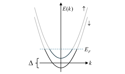
where for , respectively. Figure 1 shows the energy dispersions: two parabolas, separated by and occupied up to the Fermi energy . We note that we here assume that the magnetic field only couples to the electronic spins, not to the orbital motion; in other words, we do not consider effects related to Landau level quantization of the electron gas.
The spin-split HEG is characterized by the density and spin polarization . In 3D we find the following relations:
| (9) | |||||
| (10) |
From this, the spin-resolved Fermi wavevectors follow as
| (11) |
The corresponding relations in 2D are
| (12) | |||||
| (13) | |||||
| (14) |
A useful quantity to characterize the HEG is the Wigner-Seitz radius, defined as in 3D and in 2D. The definitions of are independent of the spin polarization.
II.3 Linear spin-density matrix response
In the following it will be convenient to use an alternative formulation of SDFT based on the spin-density matrix instead of the -based formulation of Sec. II.1. Details of the transformation between the two formulations are given in Appendix A.
The linear response equation of the spin-density matrix has the individual components
| (15) |
where is the effective spin-dependent perturbing potential (see below) and is the noninteracting response function, defined as
| (16) | |||||
Here, is the zero-temperature occupation number of the th eigenstate (0 if empty, 1 if occupied), and is a positive infinitesimal.
For spin waves we need the spin-flip response functions, and . For a spin-split HEG, these are given by
| (17) | ||||
| (18) | ||||
where and 3 in 2D and 3D, respectively, and is the zero-temperature Fermi function with respect to and using the single-particle energies of Eq. (8).
The noninteracting spin-flip response functions (17) and (18) can be evaluated analytically for the real and imaginary part, similarly to the derivation of the spin-conserving response functions of the HEG [37]. The results are presented in Appendix B.
The frequency- and spin-dependent perturbing KS potential is in general given by
| (19) |
where is the external perturbation, the linearized Hartree potential is given by
| (20) |
with the Hartree kernel , and the linearized xc potential is defined in Appendix A.2, featuring the xc kernel .
II.4 Spin Waves in a spin-polarized HEG
The excitation spectrum of any system is characterized by the condition that the response equation (15) has finite solutions in the absence of any external perturbation, i.e., . This condition can be written in a form in which an integral operator consisting of and the Hartree and xc kernels has the eigenvalue 1 [38].
For the HEG, this reduces to the condition in which the matrix has eigenvalue 1. For the xc matrix elements we use Eqs. (62)–(65) for the HEG, and Eq. (97) if the source-free correction is included. Both cases show that in a spin-polarized (para- or ferromagnetic) HEG the spin-conserving and spin-flip excitation channels are decoupled and can be considered independently of each other [37]. The spin-conserving channel includes the plasmon modes, which are dominated by classical Coulomb effects, i.e., the linearized Hartree potential (20). The spin-flip excitations, on the other hand, are solely determined by linearized xc effects.
Thus, to calculate the spin waves we can consider the matrix product
| (21) |
which leads to the condition
| (22) |
The xc kernel of the HEG in LSDA (without the SF correction) is given by
| (23) | |||||
| (24) |
where , and in the following we will abbreviate . Equation (22) then gives the following condition for spin waves:
| (25) |
This can be used to determine the spin-wave dispersion numerically.
Using condition (25) and the analytic expressions for the spin-flip Lindhard function, we can find small- expressions for the LSDA spin wave dispersion [39]:
| (26) |
| (27) |
Larmor’s Theorem [40, 41] states that in a system of identical particles with sufficiently weak magnetic field , the particles carry out a collective precession at exactly the noninteracting frequency, which is determined only by . For the HEG, this means . As shown by the small- dispersion, this is true within LSDA in both 2D and 3D.
If the SF correction is applied on top of the LSDA, see Appendix C, then the ground state of the HEG remains fundamentally unchanged since a uniform magnetic field is per definition source free. However, the linear response of the system does not remain unchanged: the xc kernels now become
| (28) | |||||
| (29) |
Equation (22) then gives a new condition:
| (30) | |||||
After simplification, this becomes
| (31) |
Using Eq. (31) and the analytic expressions for the spin-flip Lindhard function, we can find small- expressions for the SF-LSDA spin wave dispersion:
| (32) | |||
| (33) | |||
We now see that Larmor’s Theorem is violated if the SF correction is made: using , we obtain in both 2D and 3D,
| (34) |
We will investigate the severity of this violation below.
III Numerical Results and Discussion
III.1 Paramagnetic HEG
We first consider the paramagnetic case, where a uniform applied magnetic field is required to induce the spin polarization .
III.1.1 Spin-wave dispersions and Larmor’s theorem
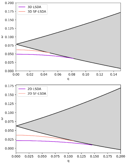
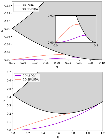
Using the conditions for LSDA spin waves and SF-LSDA spin waves, as well as the spin-flip Lindhard functions, we can solve numerically for the frequency and obtain spin wave dispersions in 2D and 3D. Examples are shown in Fig. 2, where we choose and in both cases. In 3D this implies and in 2D it implies .
The shaded areas shown in Fig. 2 are the regions of single-particle spin-flip (Stoner) excitations. The boundaries of these regions follow from the poles of Eqs. (17) or (18) for positive or negative polarization values, respectively. Here we have , and so the upper () and lower () boundaries are given by
| (35) |
The energy dispersions of the spin waves are found below the single-particle continuum. As discussed above, the SF spin wave dispersions violate the Larmor condition , and, as seen from Fig. 2, the discrepancy is substantial: the SF spin wave dispersions in 3D and 2D have similar shapes as the LSDA ones, but are significantly offset to higher frequencies.
To further quantify this observation, we introduce a parameter , which measures the relative violation of Larmor’s Theorem:
| (36) |
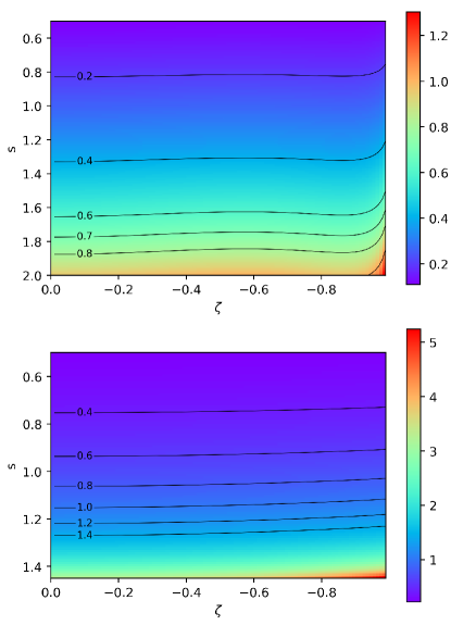
where is given in Eq. (34). depends on the HEG parameters and , as well as on the empirical scaling factor . The results are shown in Fig. 3, for =4 and and a range of values of .
Generally, a mild violation of Larmor’s Theorem would correspond to values of order . For around 1.1, we find that in 3D and in 2D, which is certainly not small. We also calculated for other values of , and found the general trend that the degree of violation of Larmor’s theorem increases with .
III.1.2 Spin-wave stiffness
A useful quantity to characterize spin-wave dispersions is the spin-wave stiffness , which is defined via the small- dispersion:
| (37) |
In other words, is a measure of the curvature of the small- limit of the spin-wave dispersion; can be read off from Eqs. (26), (27) and (32), (33), respectively.
In Fig. 4 we compare the spin-wave stiffnesses in 2D and 3D within LSDA and SF-LSDA, where we assume in the SF case. The overall behavior of as a function of and is similar with and without the SF correction; however, for given values of and , the SF-LSDA stiffness tends to be greater (i.e., more negative) than the LSDA stiffness by roughly a factor of 2–3 (in 3D) and 2.5–4 (in 2D). The reason for this is easily seen from the spin-wave dispersion curves in Fig. 2: the SF dispersions are always above the non-SF dispersions, and therefore reach the spin-flip continuum earlier. This causes the SF dispersions to bend down more rapidly, thus enhancing . Similar trends are observed for scaling factors different from 1.
III.2 Ferromagnetic HEG
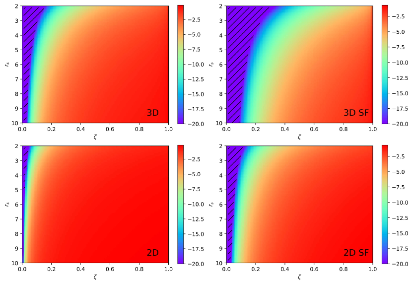
The phase diagram of the ground state of the HEG is quite rich [37]. It is know that the ground state undergoes a transition from paramagnetic to ferromagnetic for decreasing density, eventually leading to Wigner crystallization. One finds that the paramagnetic to ferromagnetic transition occurs in 3D at (using the xc functional of Ref. [42]) and in 2D at (using the xc functional of Ref. [43]). If the correlation energy of the HEG is not included, i.e., in exchange-only, then the HEG becomes ferromagnetic at much smaller values of (in 3D at and in 2D at ).
In the ferromagnetic case, the magnon dispersion of the HEG follows from Eqs. (26) and (27) by setting and :
| (38) |
| (39) |
We thus obtain a gapless dispersion with behavior at small , which is characteristic for ferromagnetic magnons.
A very different behavior is observed in the SF case. Setting and we find
| (40) |
| (41) |
These are gapless mode dispersions linear in , which is a behavior one would find in an antiferromagnet, but certainly not in the ferromagnetic HEG.
Figure 5 gives an explicit illustration, using exchange-only LSDA and SF-LSDA (since in exchange-only the HEG turns ferromagnetic for reasonably small values of ). The spin waves all start correctly at for but then approach the Stoner continuum in a different manner; the linear behavior of SF-LSDA is clearly visible.
IV Conclusions
Under certain constraints and assumptions, the xc magnetic field of SDFT can be expressed as , i.e., it can be chosen to be purely transverse. In practice, this condition does not hold for most commonly used approximations, and it is an attractive idea to enforce it by construction. This defines the SF condition, see Eq. (6). The literature suggests [31, 32, 33] that this indeed leads to improved results for the ground state of magnetic materials.
The drawback of the SF construction is that it is an ad-hoc prescription that is directly applied as a fix for a given approximation to . By contrast, the exact xc magnetic field is derived as the (unconstrained) functional derivative of the xc energy functional . This is not the case for the SF-corrected : in other words, it is not a functional derivative. While this appears to be relatively benign for the ground state, we have found it to cause serious problems if the SF construction is extended into the dynamical regime.
We have tested the SF prescription for one of the most important model systems in condensed matter, the HEG. We calculated spin-wave dispersions of the paramagnetic and ferromagnetic HEG for a broad range of densities and spin polarizations. While SF was capable of producing spin waves, it led to the violation of two exact conditions: Larmor’s theorem for the paramagnetic case, and the correct (quadratic) small- behavior of the magnons in the ferromagnetic case. While the HEG is admittedly an idealized model system, it nevertheless is very relevant for real materials. Specifically, any magnetic material which has a significant contribution to its magnetism coming from itinerant electrons requires a method that correctly describes the physics in the HEG limit.
There does not seem to be an easy way to fix these defects of the SF construction in the dynamical regime. Our study suggests that the SF construction in its present form should be limited to the magnetic ground state or to magnetic materials with localized magnetic moments. Magnetic excitations in materials with significant itinerant character should better be described using standard local or semilocal functionals. Finding an xc magnetic field functional that is source-free and yields the correct physics in both the ground state and in the dynamical regime will remain an important task for future studies.
Acknowledgements.
This work was supported by DOE Grant No. DE-SC0019109. We thank Sangeeta Sharma and Kay Dewhurst for very helpful comments.Appendix A Variables and transformations in SDFT
A.1 Densities and Kohn-Sham potentials
In Section II.1 we formulated SDFT using the density and magnetization as basic variables. Alternatively [24], SDFT can be formulated in terms of the spin-density matrix
| (42) |
For the Kohn-Sham system, the spin-density matrix is defined as , where the spin-up and spin-down components of follow from
| (43) |
Here, and are spin indices running over . The effective Kohn-Sham potential is a matrix in spin space whose xc part is defined as
| (44) |
The SDFT formulations in terms of and in terms of are physically equivalent. To transform between them, it is convenient to rearrange the basic variables as 4-component column vectors,
| (45) |
One finds [24]
| (46) |
where the transformation matrix is given by
| (47) |
with . Likewise, we can write the corresponding Kohn-Sham effective potentials and magnetic fields in 4-component vector form as
| (48) |
The connection between the two is
| (49) |
A.2 Linear response
We can formulate the frequency-dependent linear response equations within both the formulations discussed above. The density-magnetization response to a perturbing scalar potential and magnetic field is given by
| (50) |
and the spin-density-matrix response to a perturbation is given by
| (51) |
The connection between the response functions is
| (52) |
The same relations apply for the respective interacting and noninteracting response functions.
The key quantities in TD-SDFT are the linearized xc potentials, defined as follows:
| (53) | |||||
| (54) |
where the xc kernel matrices are related via
| (55) |
In the adiabatic approximation, the xc kernels are obtained from the xc energy functionals in the usual way. We have
| (56) |
where the right-hand side is evaluated at the ground-state density and magnetization , and the indices relate to , .
Likewise,
| (57) |
where the right-hand side is evaluated at the ground-state spin-density matrix .
Appendix B Spin-flip response functions of the HEG: analytic results
In this Appendix we present the results for the real and imaginary parts of the 3D and 2D spin-flip response functions of the HEG. The derivations are similar to those of the (spin-conserving) Lindhard functions of Ref. [37], and we won’t reproduce the technical details here.
B.0.1 3D case
In 3D, the real parts of and are given by
| (66) |
| (67) |
where
| (68) |
Here, the upper corresponds to the term and the lower corresponds to the term. and are the spin-resolved Fermi wavevectors, defined as , where the Fermi energy and is the spin polarization. For the calculation of the spin wave stiffness, it is helpful to use response functions to the lowest-order wavevector. That is, we let such that . In 3D, these are:
| (69) |
| (70) |
To compute and , we use the relation
| (71) |
After integration, we obtain the result:
| (72) | ||||
| (73) | ||||
B.0.2 2D case
In 2D, the real parts of and are given by
| (74) | ||||
| (75) | ||||
Expanding in the lowest-order wavevector gives the expressions:
| (76) |
| (77) |
For the imaginary part, we use the same relation (71) as in the 3D case, which gives the result:
| (78) | ||||
| (79) | ||||
Appendix C Source-free linear response formalism
In a spin-polarized HEG, the xc magnetic field
| (80) |
is uniform and hence source-free by default. To include this case in the definition of the functional (see Sec. II.1) requires some care, as discussed in Ref. [31], and the Helmholtz construction (6) is not really meaningful. In the following, we will consider a non-uniform system within the LSDA, derive the source-free construction, and only in the end take the uniform limit. As we will see, the SF construction will give rise to additional terms that do not vanish in this limit.
In LSDA, the source-free magnetic field (ignoring here the empirical scaling factor for simplicity) is given by the transverse component of the vector field:
| (81) |
or, explicitly for the LSDA,
| (82) |
where we use the short-hand notation
| (83) |
and we introduce the abbreviation
| (84) |
Now let us calculate the xc kernel . We first consider the components with , where
| (85) |
We obtain
| (86) |
where is the Levi-Civita symbol, and is the second derivative of with respect to , similarly to defined in Eq. (83). In the following, it will be convenient to express the integral over the delta function via Fourier transformation:
| (87) |
After some manipulation one then arrives at
| (88) | |||||
The first part is the collinear adiabatic LSDA, the second part is a new source-free correction.
We now consider the case of a spin-polarized HEG where , and . From Eq. (88) we then obtain a -dependent kernel:
| (89) |
We also need the derivatives with respect to the scalar density. and are unchanged with respect to the LSDA, but we get new results for , . Specifically, we find
| (90) |
and after some manipulation we end up with
| (91) | |||||
| (92) |
Again, first part is the collinear LSDA. For the HEG with , and , one then obtains the -dependent kernel
| (93) |
Let us now write the full xc kernel of the HEG, including source-free correction, in matrix form:
| (94) |
This matrix is obviously not symmetric. Since the xc kernel is defined as a second functional derivative, it should have the exact property
| (95) |
and so we would expect here that . Clearly, expression (94) does not behave like that. The reason is obvious: the source-free xc magnetic field is not variational (it is not a functional derivative). A quick and easy fix would be to symmetrize the matrix by hand, setting .
However, we are here considering a special case where the symmetry violation does not occur. Namely, we are considering spin waves that propagate perpendicular to the applied magnetic field (which sets the quantization axis). Hence, assuming that the magnetic field points along (or 3), we can set , and only consider a wavevector that is in the plane perpendicular to the external magnetic field. This simplifies things enormously, and we get
| (96) |
Transforming this using Eq. (55) finally leads to
| (97) |
References
- Barman et al. [2021] A. Barman, G. Gubbiotti, S. Ladak, A. O. Adeyeye, M. Krawczyk, J. Gräfe, C. Adelmann, S. Cotofana, A. Naeemi, V. I. Vasyuchka, B. Hillebrands, S. A. Nikitov, H. Yu, D. Grundler, A. V. Sadovnikov, A. A. Grachev, S. E. Sheshukova, J.-Y. Duquesne, M. Marangolo, G. Csaba, W. Porod, V. E. Demidov, S. Urazhdin, S. O. Demokritov, E. Albisetti, D. Petti, R. Bertacco, H. Schultheiss, V. V. Kruglyak, V. D. Poimanov, S. Sahoo, J. Sinha, H. Yang, M. Münzenberg, T. Moriyama, S. Mizukami, P. Landeros, R. A. Gallardo, G. Carlotti, J.-V. Kim, R. L. Stamps, R. E. Camley, B. Rana, Y. Otani, W. Yu, T. Yu, G. E. W. Bauer, C. Back, G. S. Uhrig, O. V. Dobrovolskiy, B. Budinska, H. Qin, S. van Dijken, A. V. Chumak, A. Khitun, D. E. Nikonov, I. A. Young, B. W. Zingsem, and M. Winklhofer, The 2021 magnonics roadmap, J. Phys.: Condens. Matter 337, 413001 (2021).
- McClarty [2022] P. A. McClarty, Topological magnons: A review, Annu. Rev. Condens. Matter Phys. 13, 171 (2022).
- Rezende [2020] S. M. Rezende, Fundamentals of Magnonics, Lecture Notes in Physics, Vol. 969 (Springer, Heidelberg, 2020).
- Savrasov [1998] S. Y. Savrasov, Linear response calculations of spin fluctuations, Phys. Rev. Lett. 81, 2570 (1998).
- Capelle et al. [2001] K. Capelle, G. Vignale, and B. L. Györffy, Spin currents and spin dynamics in time-dependent density-functional theory, Phys. Rev. Lett. 87, 206403 (2001).
- Buczek et al. [2009] P. Buczek, A. Ernst, P. Bruno, and L. M. Sandratskii, Energies and lifetimes of magnons in complex ferromagnets: A first-principle study of Heusler alloys, Phys. Rev. Lett. 102, 247206 (2009).
- Eriksson et al. [2017] O. Eriksson, A. Bergman, L. Bergqvist, and J. Hellsvik, Atomistic Spin Dynamics: Foundations and Applications (Oxford University Press, Oxford, 2017).
- Eich et al. [2018] F. G. Eich, S. Pittalis, and G. Vignale, A shortcut to gradient-corrected magnon dispersion: exchange-only case, Eur. Phys. J. B 91, 173 (2018).
- D’Amico et al. [2019] I. D’Amico, F. Perez, and C. A. Ullrich, Chirality and intrinsic dissipation of spin modes in two-dimensional electron liquids, J. Phys. D: Appl. Phys. 52, 203001 (2019).
- Tancogne-Dejean et al. [2020] N. Tancogne-Dejean, F. G. Eich, and A. Rubio, Time-dependent magnons from first principles, J. Chem. Theory Comput. 16, 1007 (2020).
- Singh et al. [2020] N. Singh, P. Elliott, J. K. Dewhurst, E. K. U. Gross, and S. Sharma, Ab-initio real-time magnon dynamics in ferromagnetic and ferrimagnetic systems, Phys. Status Solidi B 257, 1900654 (2020).
- Anderson et al. [2021] M. J. Anderson, F. Perez, and C. A. Ullrich, Spin waves in doped graphene: A time-dependent spin density functional approach to collective excitations in paramagnetic two-dimensional Dirac fermion gases, Phys. Rev. B 104, 245422 (2021).
- von Barth and Hedin [1972] U. von Barth and L. Hedin, A local exchange-correlation potential for the spin polarized case: I, J. Phys. C 5, 1629 (1972).
- Gunnarsson and Lundqvist [1976] O. Gunnarsson and B. I. Lundqvist, Exchange and correlation in atoms, molecules, and solids by the spin-density-functional formalism, Phys. Rev. B 13, 4274 (1976).
- Gidopoulos [2007] N. I. Gidopoulos, Potential in spin-density-functional theory of noncollinear magnetism determined by the many-electron ground state, Phys. Rev. B 75, 134408 (2007).
- Kübler et al. [1988] J. Kübler, K.-H. Höck, J. Sticht, and A. R. Williams, Density functional theory of non-collinear magnetism, J. Phys. F: Met. Phys. 18, 469 (1988).
- Sandratskii [1998] L. M. Sandratskii, Noncollinear magnetism in itinerant-electron systems: theory and applications, Adv. Phys. 47, 91 (1998).
- Peralta et al. [2007] J. E. Peralta, G. E. Scuseria, and M. J. Frisch, Noncollinear magnetism in density functional calculations, Phys. Rev. B 75, 125119 (2007).
- Eich and Gross [2013] F. G. Eich and E. K. U. Gross, Transverse spin-gradient functional for noncollinear spin-density-functional theory, Phys. Rev. Lett. 111, 156401 (2013).
- Scalmani and Frisch [2012] G. Scalmani and M. J. Frisch, A new approach to noncollinear spin density functional theory beyond the local density approximation, J. Chem. Theory Comput. 8, 2193 (2012).
- Bulik et al. [2013] I. W. Bulik, G. Scalmani, M. J. Frisch, and G. E. Scuseria, Noncollinear density functional theory having proper invariance and local torque properties, Phys. Rev. B 87, 035117 (2013).
- Pittalis et al. [2017] S. Pittalis, G. Vignale, and F. G. Eich, gauge invariance made simple for density functional approximations, Phys. Rev. B 96, 035141 (2017).
- Goings et al. [2018] J. J. Goings, F. Egidi, and X. Li, Current development of noncollinear electronic structure theory, Int. J. Quantum Chem. 118, e25398 (2018).
- Ullrich [2018] C. A. Ullrich, Density-functional theory for systems with noncollinear spin: orbital-dependent exchange-correlation functionals and their application to the Hubbard dimer, Phys. Rev. B 98, 035140 (2018).
- Pluhar, III and Ullrich [2019] E. A. Pluhar, III and C. A. Ullrich, Exchange-correlation magnetic fields in spin-density-functional theory, Phys. Rev. B 100, 125135 (2019).
- Desmarais et al. [2021] J. K. Desmarais, S. Komorovsky, J.-P. Flament, and A. Erba, Spin–orbit coupling from a two-component self-consistent approach. II. Non-collinear density functional theories, J. Chem. Phys. 154, 204110 (2021).
- Tancogne-Dejean et al. [2023a] N. Tancogne-Dejean, A. Rubio, and C. A. Ullrich, Constructing semilocal approximations for noncollinear spin density functional theory featuring exchange-correlation torques, Phys. Rev. B 107, 165111 (2023a).
- Tancogne-Dejean et al. [2023b] N. Tancogne-Dejean, M. Lüders, and C. A. Ullrich, Self-interaction correction schemes for non-collinear spin-density functional theory, J. Chem. Phys. 159, 224110 (2023b).
- Hill et al. [2023] D. Hill, J. Shotton, and C. A. Ullrich, Magnetization dynamics with time-dependent spin-density functional theory: significance of exchange-correlation torques, Phys. Rev. B 107, 115134 (2023).
- Pu et al. [2023] Z. Pu, H. Li, N. Zhang, H. Jiang, Y. Gao, Y. Xiao, Q. Sun, Y. Zhang, and S. Shao, Noncollinear density functional theory, Phys. Rev. Res. 5, 013036 (2023).
- Sharma et al. [2018] S. Sharma, E. U. K. Gross, A. Sanna, and J. K. Dewhurst, Source-free exchange-correlation magnetic fields in density functional theory, J. Chem. Theor. Comput. 14, 1247 (2018).
- Krishna et al. [2019] J. Krishna, N. Singh, S. Shallcross, J. K. Dewhurst, E. K. U. Gross, T. Maitra, and S. Sharma, Complete description of the magnetic ground state in spinel vanadates, Phys. Rev. B 100, 081102(R) (2019).
- Moore et al. [2024] G. C. Moore, M. K. Horton, A. D. Kaplan, S. M. Griffin, and K. A. Persson, Realistic non-collinear ground states of solids with source-free exchange correlation functional, arXiv:2310.00114 (2024).
- Capelle and Gross [1997] K. Capelle and E. K. U. Gross, Spin-density functionals from current-density functional theory and vice versa: A road towards new approximations, Phys. Rev. Lett. 78, 1872 (1997).
- Vignale and Rasolt [1987] G. Vignale and M. Rasolt, Density-functional theory in strong magnetic fields, Phys. Rev. Lett. 59, 2360 (1987).
- Dewhurst et al. [2018] J. K. Dewhurst, A. Sanna, and S. Sharma, Effect of exchange-correlation spin torque on spin dynamics, Eur. Phys. J. B 91, 218 (2018).
- Giuliani and Vignale [2005] G. F. Giuliani and G. Vignale, Quantum Theory of the Electron Liquid (Cambridge University Press, Cambridge, 2005).
- Petersilka et al. [1996] M. Petersilka, U. J. Gossmann, and E. K. U. Gross, Excitation energies from time-dependent density-functional theory, Phys. Rev. Lett. 76, 1212 (1996).
- Yosida [1996] K. Yosida, Theory of Magnetism (Springer, Berlin, 1996).
- Lipparini [2008] E. Lipparini, Modern many-particle physics, 2nd ed. (World Scientific, Singapore, 2008).
- Karimi et al. [2018] S. Karimi, C. A. Ullrich, I. D’Amico, and F. Perez, Spin-helix Larmor mode, Sci. Rep. 8, 3470 (2018).
- Perdew and Wang [1992] J. P. Perdew and Y. Wang, Accurate and simple analytic representation of the electron-gas correlation energy, Phys. Rev. B 45, 13244 (1992).
- Attaccalite et al. [2002] C. Attaccalite, S. Moroni, P. Gori-Giorgi, and G. B. Bachelet, Correlation energy and spin polarization in the 2D electron gas, Phys. Rev. Lett. 88, 256601 (2002).