Low-overhead fault-tolerant quantum computation by gauging logical operators

Abstract

Quantum computation must be performed in a fault-tolerant manner to be realizable in practice. Recent progress has uncovered quantum error-correcting codes with sparse connectivity requirements and constant qubit overhead. Existing schemes for fault-tolerant logical measurement do not always achieve low qubit overhead. Here we present a low-overhead method to implement fault-tolerant logical measurement in a quantum error-correcting code by treating the logical operator as a symmetry and gauging it. The gauging measurement procedure introduces a high degree of flexibility that can be leveraged to achieve a qubit overhead that is linear in the weight of the operator being measured up to a polylogarithmic factor. This flexibility also allows the procedure to be adapted to arbitrary quantum codes. Our results provide a new, more efficient, approach to performing fault-tolerant quantum computation, making it more tractable for near-term implementation.

Quantum error-correcting codes are an essential ingredient to protect quantum information in a quantum computer from errors due to coupling to an external environment [1, 2, 3, 4, 5, 6, 7, 8, 9]. Recent progress [10, 11, 12, 13, 14, 15, 16, 17, 18] has led to the discovery in Ref. [19] of good quantum low-density parity-check (qLDPC) codes [19, 20, 21], which have constant encoding rate and relative distance. Such codes are far more efficient at protecting large amounts of quantum information [22, 23, 24] than standard approaches based on the surface code [25, 26, 27]. An important open question is whether the advantages that good qLDPC codes offer for quantum information storage come at the cost of straightforward and efficient logical quantum information processing.

A key requirement for logical quantum gates on a quantum error-correcting code is fault tolerance – they must function in the presence of errors while maintaining protection of the encoded quantum information throughout a computation. Existing approaches to performing fault-tolerant logical quantum gates can be roughly divided into code-preserving and code-deforming.

Code-preserving gates include transversal gates [4], which act via the same operator on all physical and logical qubits, and more general locality-preserving gates [28]. The definition of locality depends on the context, a loose notion is that the set of constant weight errors should be preserved. Nontrivial code-preserving gates are synonymous with symmetries of an underlying code [29, 30, 28, 31, 32, 33, 34]. As a consequence, such gates necessitate a degree of structure to exist in said code.

Code-deforming gates are more general and allow a code to be deformed through a sequence of different codes to enact a logical gate [35, 36, 37, 38, 39, 40, 41]. Unlike code-preserving gates, code-deforming gates are generic as they do not necessitate the existence of nontrivial symmetries of the code beyond the logical operators themselves. In particular, code-deforming gates allow for the fault-tolerant measurement of logical operators [36, 37]. This opens up the possibility of implementing measurement-only quantum computation, where Clifford gates and $T$-gate injections are implemented via measurement, or Pauli based computation (PBC) [42] where a quantum circuit is compiled into a sequence of generalized magic state injections [43]. Lattice surgery is a code-deforming approach to fault-tolerant computation for the surface code that has been studied extensively [36, 44, 43, 45].

There are a number of proposals for performing fault-tolerant logical gates on qLDPC codes in the literature [46, 47, 48, 49, 50, 51, 52]. These include code-preserving gates and code-deforming gates. The most direct generalization of surface code lattice surgery is the scheme proposed in Ref. [48] where surface codes are replaced by a general qLDPC code and an auxiliary code that is similar to a patch of surface code. The auxiliary code incurs a qubit overhead of $\Theta(Wd)$ where $W$ is the weight of the logical being measured and $d$ is the code distance. For low-distance codes with $d=O(\sqrt{n})$, where $n$ is the number of physical qubits, this suffices to implement measurement-only quantum computation with qubit overhead linear in $n$. However, for higher distance codes the qubit overhead becomes super-linear, increasing to $\Theta(n^{2})$ for good codes. Furthermore, for constant-rate codes with small polynomial distances, such as hypergraph product codes [11, 12], this scheme does not suffice to implement linear qubit overhead PBC as the weight of a generic product of logical operators is expected to scale as $\Theta(n)$.

Recent work [51] solves the overhead issues in some cases by pointing out that if constant expansion exists in the Tanner graph structure of the logical operator, the overhead can be reduced significantly to $\Theta(W)$. However, this in addition requires the existence of low-weight auxiliary gauge-fixing checks.

In this work we introduce a general procedure for the fault-tolerant measurement of a logical operator in a stabilizer code by treating it as physical symmetry and gauging it via measurement [53, 54, 55]. The gauging procedure is common in the theory of condensed matter and high energy physics, it enforces a global symmetry via a product of local symmetries. Our new measurement scheme is based on the fact that the gauging transformation makes it possible to infer the measurement of a logical operator via a product of local stabilizers in a deformed code. Gauging has been employed widely in theoretical physics to construct new models and establish relationships between known models [56, 57, 58]. The connection of gauging to quantum codes has also been studied [59, 60, 61, 62, 63]. Previous work focused on gauging procedures that correspond to the simultaneous initialization and readout of all logical qubits in a code and did not consider fault tolerance. The appearance of a similar procedure in recent work on weight reduction for quantum codes hints at wider applications of gauging in quantum error correction [64, 65, 66, 67].

Here, we go beyond previous work by developing a fault-tolerant gauging measurement procedure that can precisely address arbitrary individual logical operators in a large code block. We prove that the worst-case qubit overhead of the gauging measurement procedure applied to an arbitrary Pauli operator of weight $W$ is $O(W\log^{2}W)$, a significant improvement over existing results in the literature. We further demonstrate that the flexibility inherent to the gauging measurement procedure leads to better performance than existing schemes for logical measurement [68, 51] even for small instances of Bivariate Bicycle (BB) codes [23].

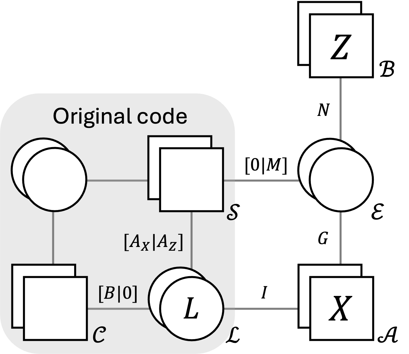
Figure 1: The Tanner graph of the deformed code can be represented compactly by creating ordered subsets of qubits (circles) and checks (squares) of $X$, $Z$, or mixed (unlabeled) type. Each edge connecting an $X$ or $Z$ check set $\mathcal{P}$ and qubit set $\mathcal{Q}$ is labeled by a binary matrix $H$ with $|\mathcal{P}|$ rows and $|\mathcal{Q}|$ columns, where $H_{ij}=1$ if and only if the $i^{\text{th}}$ check in $\mathcal{P}$ acts non-trivially on the $j^{\text{th}}$ qubit in $\mathcal{Q}$. Edges from mixed type check sets are instead labeled with a symplectic matrix $[H_{X}|H_{Z}]$ where $H_{X}$ indicates qubits acted on by $X$ and $H_{Z}$ those acted on by $Z$. The original code may not be CSS, but we assume without loss of generality that $L$, the operator being measured, is $X$-type and its qubit support is $\mathcal{L}$. Set $\mathcal{C}$ contains checks from the original code that do not have $Z$-type support on $\mathcal{L}$, while set $\mathcal{S}$ contains checks that do. Also, $\mathcal{A}$ is the set of Gauss’s law operators $A_{v}$, $\mathcal{B}$ is the set of flux operators $B_{p}$, and $\mathcal{E}$ is the set of edge qubits. Matrix $N$ specifies a cycle basis of $G$ and $M$ indicates how original stabilizers are deformed by perfect matching in $G$ (see Remark 4).

Gauging measurement— We now present the procedure to measure a logical operator via gauging. This procedure is summarized in Algorithm 1. We focus on the task of measuring a logical representative $L$ in an $[[n,k,d]]$ qLDPC stabilizer code on qubits specified by checks $\{s_{i}\}$ [4]. By choosing an appropriate basis for each qubit we ensure that $L$ is a product of Pauli-$X$ matrices without loss of generality. We view $L$ as a symmetry of the code by identifying the codespace with the groundspace of the Hamiltonan $H=-\sum_{i}s_{i}$ and noting that $L$ commutes with every stabilizer. From this point of view it is natural to project into an eigenspace of $L$ by gauging it.

To gauge $L$ we first pick a connected graph $G$ whose vertices are identified with the qubits in the support of $L$. We next introduce an auxiliary qubit on each edge of $G$, initialized in the $\ket{0}$ state. In the physics literature these edge qubits are referred to as gauge qubits. Finally, we introduce a set of Gauss’s law operators, $\mathcal{A}=\{A_{v}\}_{v\in V}$ where ${A_{v}=X_{v}\prod_{e\ni v}X_{e}}$, and project the code onto an eigenspace of each of these operators via measurement. This results in a deformed code, which is a subsystem code if the number of edge qubits exceeds the number of Gauss’s law operators. This subsystem code is gauge fixed by the choice of initial state for the edge qubits. The gauge fixed code is a stabilizer code specified by the deformed check operators of the original code and a set of flux operators $\mathcal{B}=\{B_{p}\}_{p\in C}$, where $B_{p}=\prod_{e\in p}Z_{e}$, and $p$ labels a generating set of cycles for $G$. The flux operators are obtained from a deformation of the initial single body $Z_{e}$ checks on the edge qubits. See Fig. 1 for a depiction of the Tanner graph of the deformed code.

The above gauging procedure maps the original code space into the code space of a deformed code which is known as the gauged code. To implement the eigenspace projections of the gauging procedure we rely on measuring the Gauss’s law operators [53, 54]. While the initial measurement of each Gauss’s law operator may return a random eigenvalue outcome, the product of all outcomes yields the measured eigenvalue of the logical $L$. We can return to the original code space by simply projecting onto the simultaneous $+1$ eigenspace of the $Z_{e}$ operators on all the edge qubits. To implement this step we measure $Z_{e}$ on each edge qubit. While the outcome of each measurement may be random, it is possible to find a Pauli-$X$ byproduct operator on the original qubits that can be applied to achieve the same effect as projecting onto the all $+1$ measurement outcome. This step is commonly referred to as ungauging.

Algorithm 1 Gauging measurement procedure

A Pauli stabilizer code specified by checks $\{s_{i}\}$ initialized in the physical code state $\ket{\psi}$.

A Pauli logical operator representative $L$.

A connected graph $G$ with an arbitrarily chosen vertex $v_{0}$ and an isomorphism that identifies the qubits in the support of $L$ with the vertices of $G$.

The result $\sigma=\pm 1$ of measuring $L$ and the post-measurement code state $\ket{\Psi}=\frac{1}{2}(\mathds{1}+\sigma L)\ket{\psi}$.

$\sigma\leftarrow 1$

$\ket{\Psi}\leftarrow\ket{\psi}$

$\{\omega_{e}\}_{e\in E_{G}}\leftarrow\{1\}_{e\in E_{G}}$

$\gamma\leftarrow\{\}$

for each edge $e$ in $G$ do

     $\ket{\Psi}\leftarrow\ket{\Psi}\otimes\ket{0}_{e}$ $\triangleright$ Initialize a qubit on $e$

end for

for each vertex $v$ in $G$ do

     Measure $A_{v}$ on $\ket{\Psi}$ $\triangleright$ $A_{v}=X_{v}\prod_{e\ni v}X_{e}$

     $\varepsilon\leftarrow$ Measurement result $\triangleright$ Measurement result is $\pm 1$

     $\ket{\Psi}\leftarrow\frac{1}{2}(\mathds{1}+\varepsilon A_{v})\ket{\Psi}$ $\triangleright$ Post-measurement state

     $\sigma\leftarrow\varepsilon\sigma$

end for

for each edge $e$ in $G$ do

     Measure $Z_{e}$ on $\ket{\Psi}$

     $\omega_{e}\leftarrow$ Measurement result $\triangleright$ Measurement result is $\pm 1$

     $\ket{\Psi}\leftarrow\frac{1}{2}(\mathds{1}+\omega_{e}Z_{e})\ket{\Psi}$ $\triangleright$ Post-measurement state

     Discard auxiliary qubit on $e$

end for

for each vertex $v$ in $G$ do

     $\gamma\leftarrow$ An arbitrary edge-path from $v_{0}$ to $v$

     if $\prod_{e\in\gamma}\omega_{e}=-1$ then

         $\ket{\Psi}\leftarrow X_{v}\ket{\Psi}$ $\triangleright$ Apply byproduct operator

     end if

end for

Remark 1 (Circuit implementation).

The gauging procedure can be implemented by a circuit with no additional qubits by implementing the $A_{v}$ measurements as follows. After initializing the edge qubits we perform the entangling circuit $\prod_{v}\prod_{e\ni v}CX_{v\rightarrow e}$. Next, we projectively measure $X_{v}$ on all vertices in $G$ and keep the post-measurement state. We then repeat the same entangling circuit, followed by a measurement of the edge operators $Z_{e}$ where the edge qubits are discarded.

Theorem 1 (Gauging measurement).

The gauging procedure defined in Algorithm 1 is equivalent to performing a projective measurement of $L$.

Proof.

See the supplementary material. ∎

Remark 2.

Algorithm 1 is an extremely flexible recipe due to the choice of an arbitrary graph $G$. The properties of the deformed code depend strongly on the choice of this graph. Below, we discuss desirable properties of the graph $G$ to achieve a fault-tolerant implementation of the gauging measurement with low overhead. The graph $G$ can be chosen to have additional vertices beyond the qubits in the support of a given logical operator. This is achieved by adding an auxiliary qubit, initialized in the $\ket{+}$ state, for each desired extra vertex and then gauging the desired logical operator multiplied by $X$ on each added vertex. We refer to the extra vertices as dummy vertices since they have no effect on the gauging measurement as they return the $+1$ result with certainty when $X_{v}$ is measured on them and hence they do not need to be included in practice and can be substituted for the classical value $+1$.

Remark 3 (Desiderata for $G$).

Our goals when picking a constant-degree graph $G$ are threefold. First, $G$ should contain a constant length edge-path between pairs of vertices that are in the $Z$-type support of a check from the original code. The $Z$-type support of a Pauli operator is the set of sites it acts on via $Y$ and $Z$ operators. Second, the Cheeger constant of $G$ should be at least 1, that is $h(G)\geq 1$, to ensure that $G$ is sufficiently exapnding. Third, there should be a generating set of cycles for $G$ with low weight (less than some constant). When such a graph is found the gauging measurement procedure has constant qubit overhead.

Remark 4 (Construction of a suitable $G$).

We now outline a construction that produces a graph $G$ with qubit overhead $O(W\log^{2}W)$ that satisfies the desiderata from the previous remark. First, we pick a $\mathbb{Z}_{2}$-perfect-matching of the vertices in the $Z$-type support of each check from the original code that overlaps the target logical $L$ and add an edge to $G$ for each pair of matched vertices. Second, we add edges to $G$ until $h(G)\geq 1$. This step can be performed by adding edges to $G$ at random while preserving constant degree, or by taking an existing constant degree expander graph with $h(G)\geq 1$ and adding its edges to $G$. We use $G_{0}$ to denote the graph that has been constructed thus far. Third, we add to $G$ a sufficient number of additional layers that are copies of the graph $G_{0}$ on a sequence of dummy vertices, which are connected sequentially back to the original vertices. We then add edges to the additional layers to sparsify the cycles of $G_{0}$ to achieve a desired constant weight and degree. This step is based on cellulation and the Freedman-Hastings decongestion lemma [69], and is explained in detail in the supplementary material. The Freedman-Hastings decongestion lemma establishes a $\log^{2}W$ upper bound on the number of layers needed to sparsify the cycles of an arbitrary constant degree graph $G$ with $W$ vertices when following this procedure. The lemma comes with an efficient algorithm to construct a sparsified basis of cycles, given a constant degree graph. See Fig. 2 for a depiction of the deformed code after these steps.

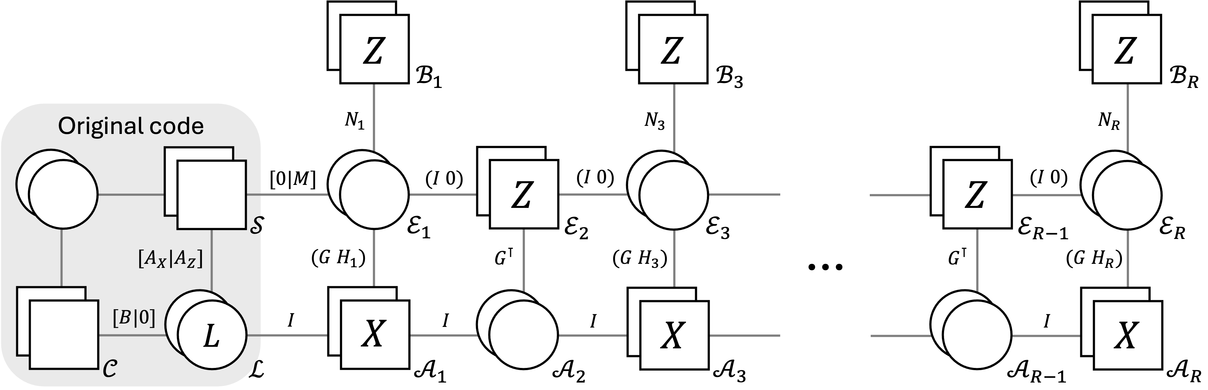
Figure 2: The Tanner graph of the complete construction including decongestion and cellulation to guarantee the deformed code is LDPC. We use the same notation as explained in Fig. 1. Additionally, $(B_{1}\text{ }B_{2})$ indicates a block matrix constructed from submatrices $B_{1}$ and $B_{2}$. We use block matrices where qubits of the left block are those on edges of the expanding graph $G$ and qubits of the right block are those added to cellulate cycles. Depending on the layer $i=1,2,\dots,R$, this cellulation is done to different elements of the cycle basis of $G$. Using $R=O(\log^{2}W)$ layers ensures the deformed code is LDPC by the decongestion lemma [69].

Remark 5 (Parallelization).

The gauging measurement can be applied to an arbitrary number of logical operators in parallel, provided that no pair of these logical operators act on a common qubit via different nontrivial Pauli operators. To maintain an LDPC code during the code deformation step it is required that only a constant number of logical operators being measured share support on any single qubit. For codes that support many disjoint logical representatives, this offers the potential of performing highly parallelized logical gates. It is also possible to trade-off time overhead for space overhead by performing $2m-1$ measurements of equivalent logical operators in parallel for $\frac{d}{m}$ rounds and then taking a majority vote to determine the classical outcome of the logical measurement.

Remark 6 (Generalizations).

The gauging measurement procedure is vastly generalizable. It can be applied to any representation of a finite group by operators that have a tensor product factorization. This representation need not form the logical operators of a quantum error-correcting code. This includes non-Pauli operators, whose measurement can produce magic states. An example of this is the measurement of Clifford operators in a topological code, see Ref. [70]. The generalization extends to qudit systems and nonabelian groups. However, for nonabelian a definite global charge is not fixed by measuring the charge locally. We leave further development of this direction to future work.

Remark 7 (Replacing $G$ with a hypergraph).

The gauging measurement procedure can also be generalized to measure a number of operators simultaneously. This procedure can be applied to measure any abelian group of operators that are describable as the $X$-type operators that commute with an auxiliary set of $k$-local $Z$-type checks. This type of group can equivalently be formulated as the kernel of a sparse linear map over $\mathbb{F}_{p}$ using the stabilizer formalism [4]. For qubits this is equivalent to replacing $G$ with a hypergraph. The generalized gauging procedure performs a code deformation by introducing a qubit for each hyperedge and measuring into new $A_{v}$ checks given by the product of $X$ on a vertex and the adjacent hyperedges.

Fault-tolerant implementation— Algorithm 1 can be implemented fault tolerantly by measuring the stabilizer checks of the original code for $d$ rounds, followed by measuring the checks of the deformed code for $d$ rounds, and finally measuring the checks of the original code for a further $d$ rounds.

Theorem 2 (Fault-tolerance).

The fault-tolerant implementation of Algorithm 1 with a suitable graph has spacetime fault-distance $d$.

Proof.

The proof follows several lemmas that are stated and proved in the supplementary material. The argument is structured as follows, the fault distance is shown to be lower bounded by the minimum of the space fault distance and the time fault distance. The time fault distance is lower bounded by the number of rounds between the start and end of the code deformation, which is chosen to be $d$. The space fault distance is lower bounded by the distance of the original code multiplied by $\min(1,h(G))$. This is because any logical in the deformed code can be cleaned such that it defines a logical of the original code. The distance reduction of the cleaning is determined by the connectivity of $G$. ∎

Remark 8.

The scaling of the fault distance holds even if the $B_{p}$ checks are measured much less often than the $A_{v}$ and $\tilde{s}_{j}$ checks. In fact, they never need to be measured directly as they can be inferred from the initialization and readout steps of the code deformation. While this is appealing for cases where the $B_{p}$ checks have high weight, it results in large detector cells and hence the code is not expected to have a threshold without further modifications. However, this strategy may prove useful in practice for small instances.

Remark 9.

The $d$ rounds of quantum error correction in the original code before and after the gauging measurement are for the purposes of establishing a proof and are overkill in practice. In a full fault-tolerant computation the number of rounds required before and after a gauging measurement depends on the surrounding operations. If the gauging measurement occurs in the middle of a large computation we expect that a constant number of rounds before and after are sufficient to ensure fault tolerance. However, this choice is expected to affect the distance and threshold depending on the surrounding operations.

Remark 10.

The circuit implementation introduced in Remark 1 leads to a different, but closely related, fault-tolerant implementation where the vertex qubits are decoupled and can be discarded during the code deformation. The main difference is that this can lead to a reduction in the distance by a constant multiple. However, this distance reduction can be avoided by adding an extra dummy vertex to divide each edge into a pair of edges.

Discussion— In this work we have introduced a method to implement low-overhead fault-tolerant quantum computation with high-distance qLDPC codes. Our method is based on the viewing a logical operator as a symmetry and gauging it via local measurements. The gauging measurement procedure allows a high degree of flexibility, making it a promising method that can be optimized for even small code instances with near-term applications. In the supplementary material we devise specific gauging measurements for examples of bivariate bicycle codes that are more efficient than all existing measurement schemes in the literature [51, 48]. The flexibility of the gauging measurement procedure can be used to recover a number of well-known existing schemes for logical measurement including surface code lattice surgery [36], the measurement scheme in Ref. [48] and the modified version in Ref. [51]. This is discussed in more detail in the supplementary material.

The progress reported in this work raises a number of directions that invite further investigation. For what families of good qLDPC codes can the gauging measurement be performed with linear qubit overhead? Can the generalization of the gauging measurement to a hypergraph be used to measure a large number of commuting but overlapping logical operators simultaneously? Can we introduce meta-checks to the generalized gauging measurement procedure to make the measurement single-shot with a constant time overhead? How should the fault-tolerant gauging measurement be decoded? We expect that a general purpose decoder based on belief propagation with ordered statistics post-processing can be used, however it should be possible to take advantage of the extra structure inherent to the procedure to find a decoder with better performance. Such a decoder could incorporate matching on the $A_{v}$ syndromes similar to the approach in Ref. [51].

The directions listed here can be interpreted as a list of desiderata for an ideal fault-tolerant logical measurement procedure: it should implement PBC, be fully parallelized, and have constant relative overhead in space and time. It remains an open question whether any fault-tolerant logical measurement can satisfy the above desiderata, or how close one can get. Even the answer to the classical analog of this question is not known.

I acknowledgements

We thank Tomas Jochym-O’Connor and Guanyu Zhu for useful discussions and Esha Swaroop for bringing our attention to the decongestion lemma. TY thanks Andrew Cross for sharing his method of using CPLEX to calculate code distances. DW thanks Lawrence Cohen for an inspiring discussion on the ferry back from Rottnest Island. This work was initiated while DW was visiting the Simons Institute for the Theory of Computing. While this work was being completed several related works appeared [51, 71, 50, 52] and we are aware of another related work [72] that is forthcoming.

Appendix A Relation to prior work

In this section we discuss how several existing schemes for logical measurement are related to gauging measurements.

Remark 11.

Lattice surgery is a widely used scheme for logical measurements on surface codes [36]. The gauging measurement can be interpreted as a direct generalization of lattice surgery as it recovers conventional lattice surgery when applied to copies of the surface code with an appropriate choice of $G$. For example, consider the logical operator $\overline{X}_{1}\otimes\overline{X}_{2}$ supported on the right and left edge of a pair of equally sized surface code blocks, respectively. Applying the gauging measurement with a choice of graph that is a ladder joining the edge qubits of the surface codes as shown in Figure. 3 results in a deformed code that is again the surface code on the union of the two patches. The final step of measuring out individual edges is the same as conventional lattice surgery. To implement a lattice surgery between surface codes that are not directly adjacent to one another, we can apply the gauging procedure with a graph that includes a grid of dummy vertices between the two edges, see Remark 2.

Interestingly, this procedure can be extended directly to measure any pair of matching logical $X$ operators on a pair of code blocks. The logical $X$ operators are further required to each have the same choice of graph $G$ which is allowed to have low expansion $h(G)<1$ but is required to satisfy the remaining two desiderata in Remark 3 for each code block. Additional bridge edges are then added between vertices in the two copies of $G$, generalizing the choice shown in Fig. 3. Similar to lattice surgery, the gauging measurement defined by such a choice of graph preserves the code distance when the individual logical $X$ operators have minimal weight and contain no sublogical operators. We remark that this procedure is similar to the joint logical measurement construction in Ref. [51]. This discussion demonstrates that the expansion condition we have used in this work is overkill in some settings. It appears that expansion is only required for subsets of qubits that are relevant to the logical operators of the codes being measured. Developing a better understanding of the neccessary expansion conditions is an interesting direction that might lead to more efficient logical measurement protocols.

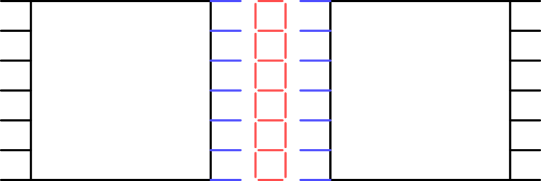
Figure 3: Applying the gauging measurement procedure to a product of $X$-type logicals on a pair of surface codes (blue edges) and choosing the graph $G$ to be a ladder (red edges) results in a standard surface code lattice surgery procedure.

Remark 12.

Shor-style logical measurement [3] involves entangling an auxiliary GHZ state to a code block via $CX$ gates that are applied transversally between the auxiliary qubits and the support of an $X$ logical. The logical is then measured by measuring $X$ on each of the auxiliary qubits and discarding them. We can perform a similar gauging measurement using a graph that has a separate dummy vertex connected by an edge to each qubit in the support of $L$, and then a connected graph on the dummy vertices. If we consider performing the gauging measurement where the edges of the connected graph on the dummy qubits are measured first, we are left with a state that corresponds to a GHZ state entangled with the support of $L$. This is similar to the Shor-style measurement where the final $X$ measurements have been commuted backwards through the $CX$ gates.

Remark 13.

A generalized version of the gauging measurement allows one to replace the auxiliary graph with a hypergraph whose adjacency matrix has the same kernel, see Remark 7. This is sufficient to capture the Cohen et al. scheme for logical measurement [48]. Consider the restriction of the $Z$-type checks to the support of an irreducible $X$ logical as was done in Ref. [48]. This defines a hypergraph of $Z$ constraints with the only nontrivial element in the kernel being the logical operator that is to be measured. Next, we add $d$ layers of dummy vertices for each qubit in the support of $L$, connect the $d$ copies of each vetex via a line graph, and join the vertices in each layer via a copy of the same underlying hypergraph. Applying the generalized gauging procedure to this hypergraph exactly reproduces the Cohen et al. measurement scheme. The logical measurement scheme from Ref. [51] can similarly be recovered by using fewer than $d$ layers of dummy vertices above. The procedures in Refs. [48, 51] for joining ancilla systems designed for irreducible logicals to measure their products can also be captured as a gauging measurement by adding edges between the graphs corresponding to the individual ancilla systems.

Remark 14.

Generalizing the gauging measurement to a hypergraph allows one to measure many logical operators simultaneously, see Remark 7. This approach can be used to implement the standard initialization of a CSS code by preparing $\ket{0}^{\otimes n}$ and measuring the $X$-type checks. This is achieved by starting with a trivial code with a dummy vertex for each $X$-type check of the CSS code and then performing the generalized gauging measurement using the hypergraph corresponding to the $Z$-type checks of the CSS code. Previous work on gauging quantum codes focused on this type of initialization measurement [53, 54, 55, 59, 60, 61, 62, 63]. In this case the ungauging step simply performs a read-out measurement of $Z$ on all qubits.

This state preparation and read-out gauging measurement procedure can be combined with another gauging measurement to implement a Steane-style measurement of a stabilizer group [73]. This can be achieved by first performing state preparation of an ancilla code block via gauging as described above. This is followed by a gauging measurement of $XX$ on pairs of matching qubits between the data code block and the ancilla code block. Finally, the ungauging step is performed to read-out $Z$ on all ancilla qubits.

Appendix B BB code examples

In this section we provide efficient gauging measurements for the bivariate bicycle (BB) codes introduced in Ref. [23]. Let $I_{r}$ be the $r\times r$ identity matrix and $C_{r}$ be the cyclic permutation matrix of $r$ items, i.e. $\langle i|C_{r}=\langle i+1\mod r|$ for all $i$. Define $x=C_{\ell}\otimes I_{m}$ and $y=I_{\ell}\otimes C_{m}$. Note $x^{\ell}=y^{m}=I_{\ell m}$ and $x^{\top}x=y^{\top}y=I_{\ell m}$.

BB codes are CSS codes using $n=2\ell m$ physical qubits divided into two sets, $\ell m$ left ($L$) qubits and $\ell m$ right ($R$) qubits. The parity check matrices of a BB code are

$$H_{X}=[A|B],\quad H_{Z}=[B^{\top}|A^{\top}],$$ (1)

where $A,B\in\mathbb{F}_{2}[x,y]$ are polynomials in the matrices $x$ and $y$. Also, $A^{\top}=A(x,y)^{\top}=A(x^{\top},y^{\top})=A(x^{-1},y^{-1})$ and likewise for $B^{\top}$. There are $\ell m$ $X$ checks and $\ell m$ $Z$ checks in this generating set, though only $(n-k)/2$ checks of either type are independent for a code encoding $k$ qubits.

The $X$ checks, $Z$ checks, $L$ qubits, and $R$ qubits are each in 1-1 correspondence with the $\ell m$ elements of

$$\mathcal{M}=\{x^{a}y^{b}:a,b\in\mathbb{Z}\}.$$ (2)

To label individual checks or qubits, we write $(\alpha,T)$ for $\alpha\in\mathcal{M}$ and $T\in\{X,Z,L,R\}$. A set of checks or qubits is more generally indicated by $(p,T)$ for a polynomial ${p\in\mathbb{F}_{2}[x,y]}$. For instance, by definition of the code, the $X$ check labeled $(\alpha,X)$ acts on qubits $(\alpha A,L)$ and $(\alpha B,R)$ while $Z$ check labeled $(\beta,Z)$ acts on qubits $(\beta B^{\top},L)$ and $(\beta A^{\top},R)$.

An $X$-type (resp. $Z$-type) Pauli acting on left qubits $(p,L)$ and right qubits $(q,R)$ for polynomials $p,q$ is more succinctly written $X(p,q)$ (resp. $Z(p,q)$). For example, the checks described previously are written $X(\alpha A,\alpha B)$ and $Z(\beta B^{\top},\beta A^{\top})$.

Gross code. The gross code is a $\llbracket 144,12,12\rrbracket$ BB code, and is so-called because a “gross” is a dozen dozens or 144. It is obtained from the BB construction by choosing $\ell=12$, $m=6$, and

$$A=x^{3}+y^{2}+y,\quad B=y^{3}+x^{2}+x.$$ (3)

We use $A_{i}$ and $B_{i}$ for $i=1,2,3$ to denote the individual monomial terms in these polynomials.

A convenient basis of logical operators for the gross code was provided in Ref. [23]. This basis is described using polynomials

$$f= 1+x+x^{2}+x^{3}+x^{6}+x^{7}+x^{8}+x^{9}$$ (4)

$$+(x+x^{5}+x^{7}+x^{11})y^{3},$$

$$g= x+x^{2}y+(1+x)y^{2}+x^{2}y^{3}+y^{4},$$

$$h= 1+(1+x)y+y^{2}+(1+x)y^{3}.$$

Then $\overline{X}_{\alpha}=X(\alpha f,0)$ and $\overline{X}^{\prime}_{\beta}=X(\beta g,\beta h)$ are logical operators for all choices of monomials $\alpha,\beta\in\mathcal{M}$. The symmetry in the BB code construction implies ${\overline{Z}_{\beta}=Z(\beta h^{\top},\beta g^{\top})}$ and $\overline{Z}^{\prime}_{\alpha}=Z(0,\alpha f^{\top})$ are also logical operators. This symmetry also means that if we construct gauging measurements for $\overline{X}_{\alpha}$ and $\overline{X}^{\prime}_{\beta}$, the same Tanner graph connectivity works for $\overline{Z}^{\prime}_{\alpha}$ and $\overline{Z}_{\beta}$, a fact that was used previously to reduce the number of ancilla systems required to measure a complete logical basis [51].

It was noted before [51, 68] that, while $\overline{X}^{\prime}_{\beta}$ can be measured by mono-layer versions of the CKBB method [48], $\overline{X}_{\alpha}$ requires several layers. This can be understood as the Tanner subgraph supported on $\overline{X}_{\alpha}$ lacking sufficient expansion [51].

The flexibility of gauging measurement allows us to measure $\overline{X}_{\alpha}$ with fewer additional qubits and checks than existing constructions. Our goal is to measure $\overline{X}_{\alpha}$ while not introducing any new checks or qubits with Tanner graph degree more than $6$ (note the 12 qubits in $\overline{X}_{\alpha}$ and the 18 adjacent $Z$ checks will necessarily become degree $7$). It happens that we can achieve this goal without decongestion or cellulation, i.e. Fig. 1 is sufficient. To specify the construction, we describe $G,M,N$.

The vertices of graph $G$ are in 1-1 correspondence with the qubits $\{(\gamma,L):\alpha\in f\}$, where $\gamma\in f$ means monomial $\gamma$ is a term in polynomial $f$. To ensure that each row of the matrix $M$ (see Fig. 1) has weight $1$, we connect two vertices $\gamma,\delta\in f$ of $G$ if qubits $(\gamma,L)$ and $(\delta,L)$ participate in the same $Z$ check. This is the case if and only if $\gamma=B_{i}^{\top}B_{j}\delta$ for some $i,j\in\{1,2,3\}$. From this step, $G$ acquires $18$ edges and is the same as it would be in the CKBB method [48].

Additional edges can now be added to $G$ to increase its expansion. This is done to ensure the deformed code has code distance equal to the original code, here distance 12. Constructing a graph with large Cheeger constant is sufficient but not necessary for this objective, so we instead randomly add edges to $G$. It is typically fast to eliminate random trials with low code distances using upper bounds provided by the BP+OSD decoder (as described in Ref. [23]). If a trial passes the BP+OSD test, then the deformed code distance can be proven to be 12 exactly with integer programming [74].

We find that four additional edges are sufficient to make a deformed code with distance 12. With vertices labeled by monomials from $f$, one choice of additional edges is

$$\begin{array}[]{cccc}(x^{2},x^{5}y^{3}),&(x^{2},x^{6}),&(x^{5}y^{3},x^{11}y^{3}),&(x^{7}y^{3},x^{11}y^{3}).\end{array}$$ (5)

As a connected graph with $12$ vertices and $22$ edges, $G$ has a minimal cycle basis consisting of $22-12+1=11$ cycles. Gaussian elimination can be used to find such a basis as the row nullspace of $G^{\top}$, i.e. find full-rank $N$ with $11$ rows such that $NG^{\top}=0$. However, because the $Z$ checks of a BB code are not all independent, the $Z$ checks in $\mathcal{B}$ implied by $N$ need not all be independent. Suppose $S$ is the sub-matrix of $H_{Z}$ containing just the rows describing $Z$ checks in $\mathcal{S}$ (i.e. checks overlapping $\overline{X}_{\alpha}$) and $C$ is the matrix describing the rest of the $Z$ checks. If $uS+vC=0$ for some vectors $u,v$, then $u,v$ identify a product of checks from sets $\mathcal{S}$ and $\mathcal{C}$ in the deformed code that is not supported on the original code and so must represent a cycle $uM$ supported on qubits $\mathcal{E}$ (possibly an empty cycle if $u=0$). Let $U=\{u:\exists v,uS+vC=0\}$. The number of redundant cycles in any cycle basis is then

$$\dim U=\mathrm{row\_nullity}(H_{Z})-\mathrm{row\_nullity}(C),$$ (6)

which evaluates to $4$ for the case at hand. Note this calculation would change if multiple logical operators were undergoing measurement simultaneously.

We therefore just need $11-4=7$ $Z$ checks in $\mathcal{B}$. We describe these checks as cycles on the vertices of $G$.

$$x^{9}\rightarrow x^{7}y^{3}\rightarrow x^{8}\rightarrow x^{9},$$

$$x^{9}\rightarrow x^{11}y^{3}\rightarrow x^{7}y^{3}\rightarrow x^{9},$$

$$x^{6}\rightarrow x^{7}\rightarrow x^{5}y^{3}\rightarrow x^{6},$$

$$x^{6}\rightarrow x^{2}\rightarrow x^{5}y^{3}\rightarrow x^{6},$$

$$x^{3}\rightarrow x^{2}\rightarrow x^{5}y^{3}\rightarrow x^{3},$$

$$x^{6}\rightarrow x^{7}\rightarrow x^{8}\rightarrow x^{7}y^{3}\rightarrow x^{6},$$

$$x\rightarrow x^{2}\rightarrow x^{5}y^{3}\rightarrow x^{11}y^{3}\rightarrow x.$$ (7)

This completes the description of the gauging measurement of $\overline{X}_{\alpha}$ in the gross code.

To summarize, Table 1 lists check weights and qubit degrees in the deformed code. Beyond the checks and qubits of the original gross code, the deformation adds $12$ $X$ checks in $\mathcal{A}$, $7$ $Z$ checks in $\mathcal{B}$, and $22$ qubits in $\mathcal{E}$. The additional checks and qubits total $41$.

$X$ checks
weight	count
4	7
5	2
6	75

$Z$ checks
weight	count
3	5
4	2
6	54
7	18

qubits
degree	count
3	8
4	9
5	5
6	132
7	12

Table 1: Check weights and qubit degrees of the deformed code for measuring $\overline{X}_{\alpha}$ in the gross code.

Double gross code. Twice as large as the gross code but with larger code distance, the $\llbracket 288,12,18\rrbracket$ double gross code is obtained from the BB code construction by taking $\ell,m=12,12$, and

$$A=x^{3}+y^{7}+y^{2},\quad B=y^{3}+x^{2}+x.$$ (8)

One set of logical operators for the double gross code are the weight-18 operators $\overline{X}_{\alpha}=X(\alpha f,0)$ for

$$f= 1+x+x^{2}+x^{7}+x^{8}+x^{9}+x^{10}+x^{11}$$

$$+(1+x^{6}+x^{8}+x^{10})y^{3}$$

$$+(x^{5}+x^{6}+x^{9}+x^{10})y^{6}+(x^{4}+x^{8})y^{9}$$ (9)

and all $\alpha\in\mathcal{M}$.

In order to measure $\overline{X}_{\alpha}=X(\alpha f,0)$ with gauging measurement, we use the construction of Fig. 1 and construct a graph $G$ with suitable properties. Just as for the gross code, each vertex $\gamma\in\mathcal{M}$ of the graph corresponds to a monomial term in $f$. An edge $(\gamma,\delta)$ is added if $\gamma=B_{i}^{\top}B_{j}\delta$ for some monomials $B_{i},B_{j}\in B$ to ensure a sparse matching matrix $M$. A total of $27$ edges are added this way.

We find we can also add an additional 7 edges to ensure the deformed code has distance $18$. Two of these edges connect the same two vertices, so the resulting graph is a multi-graph.

$$\begin{array}[]{lll}(x^{4}y^{9},x^{9}y^{6}),&(y^{3},x^{11}),&(x^{7},x^{10}y^{6}),\\ (x^{8}y^{3},x^{10}y^{6}),&(1,x^{8}),&(x^{2},x^{6}y^{3})\text{ twice}.\end{array}$$ (12)

We can then find a basis of $13$ cycles to complete the construction.

$$x^{2}\rightarrow x^{4}y^{9}\rightarrow x^{9}y^{6}\rightarrow x^{10}y^{6}\rightarrow x^{7}\rightarrow x^{6}y^{3}\rightarrow x^{2}$$

$$x^{4}y^{9}\rightarrow x^{6}y^{6}\rightarrow x^{8}y^{3}\rightarrow x^{10}y^{6}\rightarrow x^{8}y^{9}\rightarrow x^{9}y^{6}\rightarrow x^{4}y^{9}$$

$$1\rightarrow x\rightarrow y^{3}\rightarrow x^{10}y^{6}\rightarrow x^{7}\rightarrow x^{8}\rightarrow 1$$

$$1\rightarrow x\rightarrow x^{2}\rightarrow x^{6}y^{3}\rightarrow x^{8}\rightarrow 1$$

$$1\rightarrow x\rightarrow x^{2}\rightarrow y^{3}\rightarrow x^{11}\rightarrow 1$$

$$1\rightarrow x^{8}\rightarrow x^{9}\rightarrow x^{10}\rightarrow x^{11}\rightarrow 1$$

$$x^{2}\rightarrow x^{6}y^{3}\rightarrow x^{5}y^{6}\rightarrow x^{4}y^{9}\rightarrow x^{2}$$

$$x^{4}y^{9}\rightarrow x^{5}y^{6}\rightarrow x^{6}y^{6}\rightarrow x^{4}y^{9}$$

$$x^{7}\rightarrow x^{8}\rightarrow x^{6}y^{3}\rightarrow x^{7}$$

$$x^{9}\rightarrow x^{10}\rightarrow x^{8}y^{3}\rightarrow x^{9}$$

$$1\rightarrow x^{11}\rightarrow x^{10}y^{3}\rightarrow 1$$

$$x^{7}\rightarrow x^{8}y^{9}\rightarrow x^{10}y^{6}\rightarrow x^{7}$$

$$x^{2}\rightarrow x^{6}y^{3}\rightarrow x^{2}$$ (13)

Check weights and qubit degrees for this double gross code measurement are summarized in Table 2. As for the gross code, we find a deformed code with the minimal number of weight 7 checks and degree 7 qubits while requiring no higher connectivity. The deformation adds $18$ $X$ checks, $13$ $Z$ checks, and $34$ qubits, totaling $65$.

$X$ checks
weight	count
4	7
5	8
6	147

$Z$ checks
weight	count
2	1
3	5
4	1
5	3
6	120
7	27

qubits
degree	count
3	3
4	17
5	12
6	272
7	18

Table 2: Check weights and qubit degrees of the deformed code for measuring $\overline{X}_{\alpha}$ in the double gross code.

Appendix C Boundary and coboundary maps on a graph with specified cycles

In this section we introduce elementary definitions of boundary and coboundary maps on a graph $G$.

Definition 1 ($\mathbb{Z}_{2}$-Boundary and coboundary maps).

In this work we use binary vectors to indicate collections of vertices, edges, and cycles of the graph $G$. The boundary map $\partial$ on an edge vector is a $\mathbb{Z}_{2}$-linear map that is defined by its action on a single edge $\partial e=v+v^{\prime}$ where $v$ and $v^{\prime}$ are the adjacent edges of $e$. The coboundary map is given by the transpose of the boundary map $\delta=\partial^{T}$ and satisfies $\delta v=\sum_{e\ni v}e$. Given a choice of a collection of cycles in $G$ we also define a second boundary map $\partial_{2}$ whose action on a cycle is $\partial_{2}c=\sum_{e\in c}e$. Similarly, we define a second coboundary map $\delta_{2}=\partial_{2}^{T}$ which acts on a single edge as $\delta_{2}e=\sum_{c\ni e}c$.

Remark 15.

The maps $\partial_{2},$ and $\partial$ form an exact sequence if a generating set of cycles is chosen, and similarly for $\delta,\delta_{2}$. These sequences are not short exact as $\delta$ has a nontrivial kernel given by all vertices

Remark 16.

Throughout this work we abuse notation by identifying the binary vector associated to a set of vertices, edges, or cycles with the set itself. Where this is done, the meaning should be clear from context.

Appendix D Gauging measurement proof

In this section we prove Theorem 1.

Proof of Theorem 1.

Applying the gauging measurement to an initial state $\ket{\Psi}$ results in the state

$$\prod_{v}\frac{1}{2}(\mathds{1}+\varepsilon_{v}A_{v})\ket{\Psi}\ket{0}_{E}$$ (14)

up to an overall normalization. Here, $\varepsilon_{v}$ is the observed result of measuring the operator $A_{v}=X_{v}\prod_{e\ni v}X_{e}$ and $\ket{0}_{E}=\ket{0}^{\otimes E}$. Ungauging by measuring out the edge degrees of freedom in the $Z$ basis and discarding them results in the state

$$\bra{z_{e}}_{E}\prod_{v}\frac{1}{2}(\mathds{1}+\varepsilon_{v}A_{v})\ket{\Psi}\ket{0}_{E},$$ (15)

up to an overall normalization. Here, $\bra{z_{e}}_{E}=\otimes_{e}\bra{z_{e}}_{e}$ where $z_{e}$ is the observed result of measuring the operator $Z_{e}$. Next, we expand the product of projeciton operators into a sum

$$\bra{z_{e}}_{E}\frac{1}{2^{V}}\sum_{c\in C^{0}(G,\mathbb{Z}_{2})}\varepsilon(c)X_{V}(c)X_{E}(\delta c)\ket{\Psi}\ket{0}_{E},$$ (16)

where the sum is over $\mathbb{Z}_{2}$-valued 0-cochains on $G$,

$$\varepsilon(c) =\prod_{v}\varepsilon_{v}^{c_{v}},$$ (17)

$$X_{V}(c) =\prod_{v}X_{v}^{c_{v}},$$ (18)

$$X_{E}(\delta c) =\prod_{e}X_{e}^{\{\delta c\}_{e}},$$ (19)

and $\delta(\cdot)$ is the cochain map that sends a 0-chain $c$ on vertices to a 1-chain $\delta c$ on edges. Since ${\bra{z_{e}}_{E}X_{E}(\delta c)\ket{0}_{E}}$ is zero unless $z_{e}=\{\delta c\}_{e}$ on all edges, we can rewrite the ungauged state as

$$\frac{1}{2^{V}}\sum_{c\text{ s.t. }\delta c=z}\varepsilon(c)X_{V}(c)\ket{\Psi}$$

$$=\frac{1}{2^{V}}X_{V}(c^{\prime})\sum_{c\in Z^{0}(G,\mathbb{Z}_{2})}\varepsilon(c)X_{V}(c)\ket{\Psi}$$ (20)

for a fixed $c^{\prime}$ that satisfies $\delta c^{\prime}=z$ and $Z^{0}(G,\mathbb{Z}_{2})$ the group of 0-cocycles on $G$. For a connected graph $G$ there are only two elements $c\in Z^{0}(G,\mathbb{Z}_{2})$, either $c_{v}=1$ for all vertices or $c_{v}=0$ for all vertices. Hence, the ungauged state is

$$X_{V}(c^{\prime})\frac{1}{2}(\mathds{1}+\sigma L)\ket{\Psi}$$ (21)

where $L=\prod_{v}X_{v}$ is the logical operator being measured and $\sigma=\prod_{v}\epsilon_{v}$ is the observed outcome of the logical measurement. Here, $X_{V}(c^{\prime})$ is a Pauli byproduct operator determined by the observed measurement outcomes. ∎

Appendix E Properties of the deformed code

In this section we analyze the code that occurs during the application of the gauging measurement procedure to a logical operator $L$. After measuring the $A_{v}$ terms in the gauging measurement procedure we obtain a deformed code also known as the gauged code.

Definition 2 (Deformed operator).

A Pauli-operator that commutes with $L$ in the initial code can be written $P=i^{\sigma}\prod_{v\in\mathcal{S}_{X}}X_{v}\prod_{v\in\mathcal{S}_{Z}}Z_{v}$, for $\mathcal{S}_{X}$ the support of $X$ and $Y$ operators in $P$, and $\mathcal{S}_{Z}$ the support of $Y$ and $Z$ operators. Here $|\mathcal{S}_{Z}|=0\mod 2$ due to the commutativity condition. From this we define a deformed operator $\tilde{P}=s_{j}\prod_{e\in\gamma}Z_{e}$ where $\gamma$ is some edge-path in $G$ satisfying $\partial\gamma=\mathcal{S}_{Z}$. It is conventional to choose a minimum weight path.

Remark 17 (Noncommuting operators).

There is no deformed version of a Pauli-operator $P$ that does not commute with $L$. This is because there is no way to multiply such a $P$ with stabilizers $Z_{e}$ and $s_{j}$ to make it commute with all the star operators $A_{v}$ that are measured to implement the code deformation.

Remark 18 (Deformed checks).

The checks from the initial code $s_{j}=i^{\sigma}\prod_{v\in\mathcal{S}_{X}}X_{v}\prod_{v\in\mathcal{S}_{Z}}Z_{v}$ become ${\tilde{s}_{j}=s_{j}\prod_{e\in\gamma}Z_{e}}$ after the gauging measurement deformation, where $\gamma$ is some edge-path in $G$ satisfying $\partial\gamma=\mathcal{S}_{Z}$. For checks that share no $Z$-type support with $L$, i.e. those from the set $\mathcal{C}$, the deformed check is chosen to satisfy $\tilde{s}_{j}=s_{j}$. On the other hand, checks from the set $\mathcal{S}$ do share $Z$-type support with $L$ and hence are nontrivially deformed.

Lemma 1 (Deformed code).

The following form a generating set of checks for the deformed code:

• $A_{v}=X_{v}\prod_{e\ni v}X_{e}$ for all $v\in G$.

• $B_{p}=\prod_{e\in p}Z_{e}$ for a generating set of cycles $p\in G$.

• $\tilde{s}_{i}=s_{i}\prod_{e\in\gamma}Z_{e}$ for all checks in the input code $s_{i}$

Proof.

The $A_{v}$ operators become checks as they are measured during the gauging process. The $B_{p}$ operators originate from the $Z_{e}$ stabilizers on all edge qubits at the initialization step. For a product of these edge stabilizers to remain a check after measuring the $A_{v}$ operators it must commute with all $\prod_{e\ni v}X_{e}$ operators. This is equivalent to the product being over edges in a cycle $\gamma$ that satisfies $\partial\gamma=0$. Similarly, the $\tilde{s}_{i}$ operators arise from products of $s_{i}$ and $Z_{e}$ stabilizers from the initialization step that commute with all $A_{v}$ operators. This commutation condition is equivalent to the product of $Z_{e}$ operators over an edge-path $\gamma$ satisfying $\partial\gamma=\mathcal{S}_{Z}$. ∎

Remark 19.

By counting the qubtis and checks, it is simple to see that the dimension of the codespace is only reduced by a single qubit, corresponding to the logical $L$ that is measured by the gauging deformation. A total of $|E_{G}|$ new qubits are introduced along with $|V_{G}|$ new independent X-type checks and a number of new independent $Z$-type checks that is equal to $C$, the number of generating cycles of $G$. We then have $|E_{G}|-C-|V_{G}|=-1$ by counting. A simple example demonstrating the intuition behind the above formula is given by the cycle graph where $|E_{G}|=|V_{G}|$ and $C=1$. This provides an alternative method to Theorem 1 to see that no logical information is lost beyond the measurement of $L$.

Remark 20 (Freedom in defining deformed checks).

There is a large degree of freedom when specifying a generating set of checks in the deformed code. If we fix the choice of $A_{v}$ and $s_{i}$ checks, then the freedom can be associated to choosing edge-paths $p$ and $\gamma$. These choices do not affect the code space, as the $B_{p}$ operators for any generating set of cycles in $G$ generate the same algebra. Furthermore, the $\tilde{s}_{j}$ operator for two different choices of path $\gamma$ are related by multiplication with $B_{p}$ operators. In practice we aim to choose a set of paths $p$ and $\gamma$ that result in a set of checks with minimal weight and degree.

Definition 3 (Cycle-sparsified graph $\bar{\bar{G}}$).

Given a graph $G$ and a constant $c$ we call the cycle-degree, a cycle-sparsification of $G$ is a new graph that is built by adding edges to copies of $G$ numbered $0,\dots,R$. One type of additional edges connect each vertex to its copy in the subsequent layer. The other type of additional edges cellulate a cycle into triangles by connecting vertices as follows $\{(1,N-1),(N-1,2),(2,N-2),(N-2,3),\dots\}$ following an ordering of the vertices as they are visited when the cycle is traversed, see Figure 4. The cycle-sparsified graph has one copy of each chosen generating cycle cellulated, and the number of cycles any edge participates in must be $\leq c$ for some constant $c$. We use $R_{G}^{c}$ to denote the minimal number of layers to achieve a cycle-sparcification of $G$ with constant $c$. In this work we treat the $0$ layer as the original graph and follow a convention where none of the cycles in layer $0$ are cellulated.

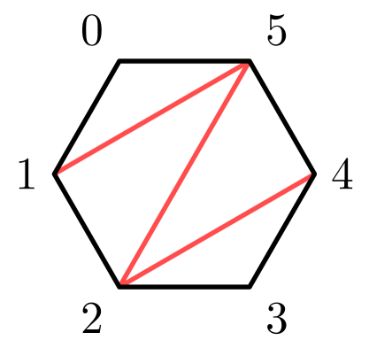
Figure 4: Cellulating a weight-six cycle (black) into a union of triangles by adding additional edges (red).

Remark 21.

Above we have chosen to cellulate the cycles into triangles as they have minimal weight. A similar procedure applies for squares, or even arbitrary polygons, which need not have a uniform number of edges. Using squares is natural in the sense that square cycles already appear between layers in the cycle-sparsified graph.

Remark 22.

For a constant degree graph there are $\Theta(|V_{G}|)$ cycles in a minimal generating set. For a random expander graph, making an appropriate choice, almost all generating cycles are expected to be of length $O(\log|V_{G}|)$. In this case we expect a cycle-degree of $O(\log|V_{G}|)$ and a number of layers $R_{G}^{c}=O(\log|V_{G}|)$ required for cycle-sparsification. We remark that the decongestion lemma [69] establishes a worst-case bound $R_{G}^{c}=O(\log^{2}|V_{G}|)$ for cycle-sparsification of a constant degree graph, see Remark 4. On the other hand, for some cases of the gauging measurement no sparsification is required, or more generally $R_{G}^{c}=O(1)$. It would be interesting to understand the conditions under which this occurs.

Remark 23 (Sparsified deformed checks).

When choosing a generating set of checks in a deformed code based on a cycle-sparsification of $G$ we take advantage of the layered structure. The basis of cycles, and corresponding $B_{p}$ terms, are picked to have weight $\leq 4$. This is achieved by using a generating set given by squares that connect each adjacent pair of copied edges, and the edges between the associated copied vertices, and the triangles that cellulate each cycle from the original generating set for $G$. The paths for the deformed $\tilde{s}_{i}$ checks remain unchanged in the sense that they are all routed through the $0$ layer. Assuming $G$ has been chosen such that the length of all paths are upper bounded by a constant $\kappa$, see Remark 3, this ensures the degree-sparsity of any edge in layer $0$. This is because there is a constant upper bound $2(\text{deg})^{\kappa}$ on the number of constant length paths that can reach a given edge, assuming $G$ has constant degree, and there are a constant number of checks, upper bounded by the check degree of the original code, that can be attached to a path at each vertex. It is possible to further sparsify the deformed checks by routing their paths into additional layers. We do not focus on this here as it is not required to achieve constant degree.

Lemma 2 (Space distance).

The distance of the deformed code satisfies $d^{*}\geq\min(h(G),1)d$, where $h(G)$ is the Cheeger constant of $G$ and $d$ is the distance of the original code.

Proof.

A logical operator on the deformed code can be written as $L^{\prime}=(i)^{\sigma}L_{X}^{V}L_{Z}^{V}L_{X}^{E}L_{Z}^{E}\tilde{L}$. Here $\tilde{L}$ captures the support of $L^{\prime}$ that does not intersect the gauged logical, $\mathcal{S}_{X}$ denotes the $X$ support of $L^{\prime}$, ${L_{X}^{V}=\prod_{v\in\mathcal{S}_{X}\cap V_{G_{0}}}X_{v}}$ captures the intersection of the $X$ support of $L^{\prime}$ with the gauged logical, ${L_{X}^{E}=\prod_{v\in\mathcal{S}_{X}\cap E_{\bar{\bar{G}}}}X_{e}}$ captures the $X$ support of $L^{\prime}$ on the edges introduced by the gauging procedure, and similarly for $Z$.

First, we consider the $X$-type component of the logical operator $L^{\prime}$. The logical operator must commute with the $B_{p}$ checks by definition, hence ${\mathcal{S}_{X}^{E}=\mathcal{S}_{X}\cap E_{\bar{\bar{G}}}}$ is a 1-cocycle on the graph $\bar{\bar{G}}$ as it satisfies ${\delta_{2}\mathcal{S}_{X}^{E}=0}$. Since the $B_{p}$ terms are defined on a generating set of cycles we have that the sequence formed by $\delta,\delta_{2}$ is exact, see Remark 15. Hence, $\mathcal{S}_{X}^{E}=\delta\tilde{\mathcal{S}}_{X}^{V}$ for some set of vertices $\tilde{\mathcal{S}}_{X}^{V}\subset V_{\bar{\bar{G}}}$. From this we have ${L_{X}^{E}=\overline{L}_{X}^{V}\prod_{v\in\tilde{\mathcal{S}}_{X}^{V}}A_{v}}$, where ${\overline{L}_{X}^{V}=\prod_{v\in\tilde{\mathcal{S}}_{X}^{V}\cap G_{0}}X_{v}}$. In the definition of $\overline{L}_{X}^{V}$, the product of operators is over vertices in $G_{0}$ since the vertices in other layers are dummy vertices which do not support qubits. We now have another logical representative that is equivalent to $L^{\prime}$, given by ${\overline{L}=i^{\sigma}L_{X}^{V}\overline{L}_{X}^{V}L_{Z}^{V}L_{Z}^{E}\tilde{L}=L^{\prime}\prod_{v\in\tilde{\mathcal{S}}_{X}^{V}}}A_{v}$.

Next, we consider the $Z$-type component of the logical operator $L^{\prime}$. We first point out that the deformed checks $\tilde{s}_{i}$ are given by the original checks, potentially multiplied with some $Z_{e}$ operators. Similarly, the equivalent logical operator $\overline{L}$ is some operator on the original qubits potentially multiplied by $Z_{e}$ operators.

From this we can see that the equivalent logical operator restricted to the qubits of the original code ${\overline{L}|_{V}=i^{\sigma}L_{X}^{V}\overline{L}_{X}^{V}L_{Z}^{V}\tilde{L}}$ must be a logical operator of the original code. This is because it must commute with the deformed checks, and since the additional operators on the edge qubits in the deformed checks are all of the form $Z_{e}$ they play no role in the commutation relations. From this we see that the full equivalent logical operator $\overline{L}$ is obtained from the restricted logical $\overline{L}|_{V}$ via the gauging code deformation.

Hence, any logical in the deformed code is equivalent to a logical on the original code $\overline{L}|_{V}$ potentially multiplied by some $Z_{e}$ operators. The weight of any nontrivial logical on the original code, such as $\overline{L}|_{V}$, is lower bounded by the distance $d$. Hence, the weight of the unrestricted logical $\overline{L}$ is also lower bounded by $d$. Furthermore, we can construct $\overline{L}$ to have support on no more than half the vertex qubits $\leq\frac{|V_{G}|}{2}$ by optionally multiplying $L^{\prime}$ with the stabilizer $\prod_{v\in V_{\bar{\bar{G}}}}A_{v}$.

We now lower bound the relative change in operator weight, induced by the equivalence under multiplication with vertex stabilizers that convert the deformed logical $\overline{L}$ back to the logical $L^{\prime}$, by the Cheeger constant $h(G)$ of a single layer of the graph $G$. For a single layer of $G$, where cycle-sparsification is not applied, this step is straightforward. In the worst case, multiplication with $\prod_{v\in\tilde{\mathcal{S}}_{X}^{V}}A_{v}$ to convert $\overline{L}$ to $L^{\prime}$ removes the support on the vertex set $\tilde{\mathcal{S}}_{X}^{V}$ and adds support on the edge coboundary set $\delta\tilde{\mathcal{S}}_{X}^{V}$. Then we apply $|\delta\tilde{\mathcal{S}}_{X}^{V}|\geq h(G)|\tilde{\mathcal{S}}_{X}^{V}|$ to achieve the distance bound on the logical $L^{\prime}$.

For a cycle-sparsified graph $\bar{\bar{G}}$ this step is more complicated. We partition the vertices in $\tilde{\mathcal{S}}_{X}^{V}\cap G_{0}$ into two types. The first type are the vertices for which not all copies of $v$ appear in $\tilde{\mathcal{S}}_{X}^{V}$. The second type are the vertices for which all copies of $v$ appear in $\tilde{\mathcal{S}}_{X}^{V}$. For a vertex of the first type, multiplication with $A_{v}$ stabilizers for $v\in\tilde{\mathcal{S}}_{X}^{V}$ leaves the support of an $X$ operator on at least one edge that connects copies of that vertex. For the second type of vertices, multiplication with $A_{v}$ stabilizers for $v\in\tilde{\mathcal{S}}_{X}^{V}$ cleans the support into the adjacent edges on all copies of $G$ and potentially some additional edges introduced to cellulate cycles. We focus on the set of type-two vertices and notice that, after cleaning, the support on the boundary edge set cannot be fully cancelled by any adjacent vertices that have been partially cleaned. This is because for any edge, and its set of copies, that is in the coboundary edge set of the fully cleaned vertices, at least one copy of the edge must support an $X$ operator. This follows from the fact that the product of $A_{v}$ terms on the adjacent vertex, and its copies, must miss at least one of the copies of $G$ by assumption. Since the combined size of the type-one and type-two vertex sets can be taken $\leq\frac{|V_{G}|}{2}$ we can use the Cheeger constant $h(G)$ to bound the relative size of the coboundary edge set to the type-two vertex set. Finally, as at least one copy of each edge in the coboundary of the type-two vertices has $X$ support, the relative weight of $L^{\prime}$ and $\overline{L}$ is also lower bounded by $h(G)$. This is a worst case bound that is saturated for $X$-type logical operators when there is only a single copy of $G$. ∎

Remark 24.

Picking a graph with Cheeger constant 1 is optimal in the sense that it leads to no reduction in the distance and a larger Cheeger constant does not improve the distance as the logicals can be cleaned onto the vertices.

Remark 25.

The above provides another way to see that the code deformation preserves all quantum information besides the measurement of the desired logical. This is because it defines a 1-1 map between logical operators in the deformed code and logical operators in the original code that commute with the logical that is being gauged. In this mapping, operators that are equivalent to the logical being gauged are mapped to stabilizers in the deformed code while all distinct logicals that commute with the logical being gauged remain nontrivial as the algebra they generate is preserved under the gauging map.

Appendix F Fault-tolerant gauging measurement procedure

In this section we provide further details about the fault-tolerant gauging measurement procedure. We follow the general approach to fault tolerance via repeated measurements introduced in Ref. [27], and borrow some terminology from Ref. [75]. The procedure begins at time $t_{0}$ followed by at least $d$ rounds of syndrome measurements in the original $[[n,k,d]]$ code. Next, there is a code deformation step at time $t_{i}$ followed by at least $d$ rounds of syndrome measurements in the deformed code. Finally, there is another code deformation step at time $t_{o}$ back to the original code, followed by at least $d$ rounds of syndrome measurements in the original code.

Remark 26.

We use a convention for labelling time steps that has check measurements occurring with an offset of half from an integer. With this convention detectors and space errors are associated to integer time steps, while measurement errors are associated to integer + half time steps. The initial gauging code deformation measurements are made at time step $t_{i}+\frac{1}{2}$ and the final ungauging code deformation measurements are made at time step $t_{o}+\frac{1}{2}$.

Definition 4 (Space and time faults).

A space-fault is a Pauli error operator that occurs on some qubit during the implementation of the gauging measurement. A time-fault is a measurement error where the result of a measurement is reported incorrectly during the implementation of the gauging measurement. A general spacetime fault is a collection of space and time faults.

Remark 27.

For the purposes of our discussion, we consider state misintialization faults to be time-faults that are equivalent to space-faults by decomposing them into a perfect initialization followed by an error operator.

Definition 5 (Detectors).

A detector is a collection of state initializations and measurements that yield a deterministic result, in the sense that the product of the observed measurement results must be $+1$ independent of the individual measurement outcomes, if there are no faults in the procedure.

Definition 6 (Syndrome).

The syndrome caused by a spacetime fault is defined to be the set of detectors that are violated in the presence of the fault. That is, the set of detectors that do not satisfy the constraint that the observed measurement results multiply to $+1$ in the presence of the fault.

Lemma 3 (Spacetime code).

The following form a generating set of the local detectors in the fault-tolerant gauging measurement procedure:
For $t<t_{i}$ and $t>t_{o}$

• $s_{j}^{t}$ which is given by the collection of repeated $s_{j}$ checks in the original code at times $t-\frac{1}{2},t+\frac{1}{2}$.

For $t_{i}<t<t_{o}$

• $A_{v}^{t}$ which is defined by the repeated measurement of the $A_{v}$ check in the deformed code at times ${t-\frac{1}{2},}{t+\frac{1}{2}}$.

• $B_{p}^{t}$ which is defined similarly for the $B_{p}$ check at times $t-\frac{1}{2},t+\frac{1}{2}$.

• $\tilde{s}_{j}^{t}$ which is defined similarly for the deformed check $\tilde{s}_{j}$ at times $t-\frac{1}{2},t+\frac{1}{2}$.

For $t=t_{i}$

• $B_{p}^{t}$ which is given by the measurement of $B_{p}$ at time $t_{i}+\frac{1}{2}$ together with the initialization of the edge qubits $e\in p$ in the $\ket{0}_{e}$ state at time $t_{i}-\frac{1}{2}$.

• $\tilde{s}_{j}^{t_{i}}$ which is given by the measurement of $\tilde{s}_{j}$, and the initialization of the edge qubits $e\in\gamma$ in the $\ket{0}_{e}$ state, at time $t_{i}-\frac{1}{2}$, and the measurement of $\tilde{s}_{j}$ at time $t_{i}+\frac{1}{2}$

For $t=t_{o}$

• $B_{p}^{t}$ which is given by the measurement of $B_{p}$ at time $t_{o}-\frac{1}{2}$ and the measurement of $Z_{e}$ on the edge qubits $e\in p$ at time $t_{o}+\frac{1}{2}$

• $\tilde{s}_{j}^{t_{o}}$ which is given by the measurement of $\tilde{s}_{j}$ at time $t_{o}-\frac{1}{2}$, together with the measurement of $Z_{e}$ on the edge qubits $e\in\gamma$, and $s_{j}$ at time $t_{o}+\frac{1}{2}$

Proof.

Away from the initial and final steps of the code deformation, the fault-tolerant gauging measurement procedure consists of repeatedly measuring the same checks. In this setting any local detector must contain a pair of measurements of the same check. This step assumes there are no local relations in the original code, see the remark below. Any detector formed by the measurement of the same check at times $(t,t+\kappa),$ can be decomposed into detectors at time steps $(t,t+1)$, $(t+1,t+2),\dots,$ $(t+\kappa-1,t+\kappa)$. During the code deformation there are also detectors that involve the initialization of the edge qubits, and their final read-out. Due to the measurement of $A_{v}$ terms during the code deformation, any detector involving the initialization of edge qubits in the $Z$ basis must include a collection of edge qubits that corresponds to a product of $B_{p}$ and $\tilde{s}_{j}$ checks. A similar statement holds for detectors that involve the read-out of edge qubits in the $Z$ basis. Any such detector can be decomposed into one of the detectors involving edges at time $t_{i}$ or $t_{o}$ listed above, combined with repeated measurement checks. Local detectors that cross the $t_{i}$ or $t_{f}$ deformation steps must involve a check $s_{j}$ from the original code at some time step before or after the deformation, along with a deformed version $\tilde{s_{j}}$. Such a detector can be decomposed into repeated measurement detectors, and one of the detectors involving edge qubits introduced above. ∎

Remark 28 (Space-only detectors).

When stating the above lemma, we have assumed there are no local detectors formed by collections of checks at a single time step. Such detectors occur in codes with local relations, or meta-checks, and are useful for single-shot quantum error correction. The fault-tolerant gauging measurement procedure can be applied to codes with local relations. If such local relations are present, it is simple to modifty the above lemma to include the space-only local detectors at each time step. However, we have chosen not to focus on such codes as the single-shot property of these code does not help reduce the time overhead of the gauging logical measurement when our current scheme is used.

Remark 29 (Initial and final boundary conditions).

Following Ref. [76], we use the convention that the initial and final round of stabilizer measurements are perfect. This is to facilitate a clean statement of our results and should not be taken literally. The justification for why this convention does not fundamentally change our results is due to the $d$ rounds of error correction in the original code before and after the gauging measurement. This ensures that any error process that involves both the gauging measurement and the initial or final boundary condition must have distance greater that $d$. In practice the gauging measurement is intended to be one component of a larger fault-tolerant quantum computation which determines the appropriate realistic boundary conditions to use.

Remark 30 (Spacetime syndromes).

The syndrome of a fault is the set of detectors it causes to have result $-1$. We say that the fault violates these detectors. The faults can be organized according to the kind of syndrome they create:
For $t<t_{i}$ and $t>t_{o}$

• A Pauli $X_{v}$ (or $Z_{v}$) operator fault at time $t$ violates the $s_{j}^{t}$ detectors for all $s_{j}$ checks that do not commute with $X_{v}$ (or $Z_{v}$).

• An $s_{j}$-measurement fault at time $t+\frac{1}{2}$ violates the detectors $s_{j}^{t}$ and $s_{j}^{t+1}$.

For $t_{i}<t<t_{o}$

• A Pauli $X_{v}$ operator fault at time $t$ violates the $\tilde{s}_{j}^{t}$ detectors for all $\tilde{s}_{j}$ checks that do not commute with $X_{v}$.

• A Pauli $Z_{v}$ operator fault at time $t$ violates the $A_{v}^{t}$ detector and the $\tilde{s}_{j}^{t}$ detectors for all $\tilde{s}_{j}$ checks that do not commute with $Z_{v}$.

• A Pauli $X_{e}$ operator fault at time $t$ violates the $B_{p}^{t}$ detectors for all $p\ni e$ and the $\tilde{s}_{j}^{t}$ detectors for all $\tilde{s}_{j}$ checks that anticommute with $X_{e}$

• A Pauli $Z_{e}$ operator fault at time $t$ violates the $A_{v}$ detectors for $v\in e$.

• A $\tilde{s}_{j}$-measurement fault at time $t+\frac{1}{2}$ violates the detectors $\tilde{s}_{j}^{t}$ and $\tilde{s}_{j}^{t+1}$.

• An $A_{v}$-measurement fault at time $t+\frac{1}{2}$ violates the detectors $A_{v}^{t}$ and $A_{v}^{t+1}$.

• A $B_{p}$-measurement fault at time $t+\frac{1}{2}$ violates the detectors $B_{p}^{t}$ and $B_{p}^{t+1}$

For $t=t_{i}$

• A Pauli $X_{v}$ (or $Z_{v}$) operator fault at time $t$ violates the $\tilde{s}_{j}^{t}$ detectors for all $\tilde{s}_{j}$ checks that do not commute with $X_{v}$ (or $Z_{v}$)

• A Pauli $X_{e}$ operator fault at time $t$ violates the $B_{p}^{t}$ detectors for all $p\ni e$ and the $\tilde{s}_{j}^{t}$ detectors for all $\tilde{s}_{j}$ checks that anticommute with $X_{e}$

• A $\ket{0}_{e}$ initialization fault at time $t-\frac{1}{2}$ is equivalent to a Pauli $X_{e}$ operator fault at time $t$ and so violates the same detectors.

• A $\tilde{s}_{j}$-measurement fault at time $t+\frac{1}{2}$ violates the detectors $\tilde{s}_{j}^{t}$ and $\tilde{s}_{j}^{t+1}$.

• An $A_{v}$-measurement fault at time $t+\frac{1}{2}$ violates the detector $A_{v}^{t+1}$.

• A $B_{p}$-measurement fault at time $t+\frac{1}{2}$ violates the detectors $B_{p}^{t}$ and $B_{p}^{t+1}$

For $t=t_{o}$

• An $X_{v}$ (or $Z_{v}$) Pauli operator fault at time $t$ violates the $\tilde{s}_{j}^{t}$ detectors for all $\tilde{s}_{j}$ checks that do not commute with $X_{v}$ (or $Z_{v}$)

• A Pauli $X_{e}$ operator fault at time $t$ violates the $B_{p}^{t}$ detectors for all $p\ni e$ and the $\tilde{s}_{j}^{t}$ detectors for all $\tilde{s}_{j}$ checks that anticommute with $X_{e}$

• A $Z_{e}$-measurement read-out fault at time $t+\frac{1}{2}$ is equivalent to a Pauli $X_{e}$ fault at time $t$ and so violates the same detectors.

• An $s_{j}$-measurement fault at time $t+\frac{1}{2}$ violates the detectors $\tilde{s}_{j}^{t}$ and $s_{j}^{t+1}$.

• An $A_{v}$-measurement fault at time $t-\frac{1}{2}$ violates the detector $A_{v}^{t-1}$.

Remark 31 (Syndrome mobility).

For $t<t_{i}$ and $t>t_{o}$ the syndromes can be created and moved around the code by Pauli errors, and propagated forwards or backwards in time via measurement errors, as usual. For $t_{i}<t<t_{o}$ Pauli errors on vertex qubits behave similarly, with the exception that $Z_{v}$ errors cause additional $A_{v}$ syndromes. Pauli $Z_{e}$ errors on edge qubits form strings that move the $A_{v}$ syndromes along edge-paths in the graph $G$. Pauli $X_{e}$ errors on edge qubits produce $B_{p}$ syndromes and can also produce clusters of $\tilde{s}_{j}$ syndromes that cannot be generated by Pauli errors on the vertex qubits alone. Again measurement errors can propagate syndromes forwards and backwards in time. At the gauging and ungauging time steps $t=t_{i}$ and $t=t_{o}$, respectively, $A_{v}$ syndromes can condense that is be created or destroyed at the time slices where the $A_{v}$ stabilizer measurements start or end. On the other hand, $B_{p}$ and $\tilde{s}_{j}$ errors can propagate through the gauging and ungauging time steps by mapping into an error caused by Pauli operators on the vertices alone up to multiplication with spacetime stabilizers including $A_{v}$ operators, see Lemma 4.

Definition 7 (Spacetime logical fault).

A spacetime logical fault is a collection of space and time faults that does not violate any detectors.

Definition 8 (Spacetime stabilizer).

A spacetime stabilizer is a trivial spacetime logical fault in the sense that it is a collection of space and time faults that does not violate any detectors and does not affect the result of the gauging measurement procedure.

Lemma 4.

The following form a generating set of local spacetime stabilizers:
For $t<t_{i}$ and $t>t_{o}$

• A stabilizer check operator $s_{j}$ at time $t$.

• A pair of Pauli $X_{i}$ (or $Z_{i}$) faults at times $t,t+1,$ together with measurement faults on all checks $s_{j}$ that do not commute with $X_{i}$ (or $Z_{i}$) at time $t+\frac{1}{2}$.

For $t_{i}<t<t_{o}$

• A stabilizer check operator $\tilde{s}_{j}$, $A_{v}$, or $B_{p}$, at time $t$.

• A pair of vertex Pauli $X_{v}$ faults at times $t,t+1,$ together with measurement faults on all checks $\tilde{s}_{j}$ that do not commute with $X_{v}$ at time $t+\frac{1}{2}$.

• A pair of vertex Pauli $Z_{v}$ faults at times $t,t+1,$ together with measurement faults on $A_{v}$ and all checks $\tilde{s}_{j}$ that do not commute with $Z_{v}$ at time $t+\frac{1}{2}$.

• A pair of edge Pauli $X_{e}$ faults at times $t,t+1,$ together with measurement faults on checks $B_{p}$ with $p\ni e$ and all checks $\tilde{s}_{j}$that do not commute with $X_{e}$ at time $t+\frac{1}{2}$.

• A pair of edge Pauli $Z_{e}$ faults at times $t,t+1,$ together with measurement faults on checks $A_{v}$ with $v\in e$ at time $t+\frac{1}{2}$.

For $t=t_{i}$

• A stabilizer check operator $s_{j}$ or $Z_{e}$ at time $t$.

• A pair of vertex Pauli $X_{v}$ faults at times $t,t+1,$ together with measurement faults on all checks $\tilde{s}_{j}$ that do not commute with $X_{v}$ at time $t+\frac{1}{2}$.

• A pair of vertex Pauli $Z_{v}$ faults at times $t,t+1,$ together with measurement faults on $A_{v}$ and all checks $\tilde{s}_{j}$ that do not commute with $Z_{v}$ at time $t+\frac{1}{2}$.

• A pair of edge Pauli $X_{e}$ faults at times $t,t+1,$ together with measurement faults on checks $B_{p}$ with $p\ni e$ and all checks $\tilde{s}_{j}$that do not commute with $X_{e}$ at time $t+\frac{1}{2}$.

• A $\ket{0}_{e}$ initialization fault at time $t-\frac{1}{2}$ together with a Pauli $X_{e}$ fault at time $t$.

• A Pauli $Z_{e}$ edge fault at time $t+1$ together with a pair of $A_{v}$ measurement faults for $v\in e$ at time $t+\frac{1}{2}$.

For $t=t_{o}$

• A stabilizer check operator $\tilde{s}_{j}$, $A_{v}$, or $B_{p}$ at time $t$.

• A pair of vertex Pauli $X_{v}$ faults at times $t,t+1,$ together with measurement faults on all checks $s_{j}$ that do not commute with $X_{v}$ at time $t+\frac{1}{2}$.

• A pair of vertex Pauli $Z_{v}$ faults at times $t,t+1,$ together with measurement faults on all checks $s_{j}$ that do not commute with $Z_{v}$ at time $t+\frac{1}{2}$.

• A Pauli $X_{e}$ edge fault at time $t,$ together with a measurement fault on check $Z_{e}$ at time $t+\frac{1}{2}$.

• A Pauli $Z_{e}$ edge fault at time $t$.

• A Pauli $Z_{e}$ edge fault at time $t-1$ together with a pair of $A_{v}$ measurement faults for $v\in e$ at time $t-\frac{1}{2}$.

Proof.

Any nonempty local spacetime stabilizer must involve a Pauli operator, or equivalent initialization or read-out error, as otherwise the stabilizer would have to include measurement errors on all repeated measurements of some check. If a nontrivial local spacetime stabilizer contains a Pauli operator at some time, it must be a space stabilizer or contain a Pauli operator at another time, or an equivalent state intialization or measurement read-out error. The product of the Pauli operators from all time steps involved must itself be a space stabilizer, where we are treating initialization and read-out errors as equivalent to some Pauli operator error. Any local spacetime fault of this form can be constructed from a product of the spacetime stabilizers introduced above by first reconstructing the operators at the earliest time step at the cost of creating matching operators at the next time step, and so on until the final time step, where the product of the operators must now become trivial. This leaves a local spacetime stabilizer with only measurement errors, which must also be trivial. Hence, the original fault pattern is a product of the introduced spacetime stabilizers as claimed. ∎

Definition 9 (Spacetime fault-distance).

The spacetime fault distance is the weight, counted in terms of single-site Pauli errors and single measurement errors, of the minimal collection of faults that does not violate any detectors and is not a spacetime stabilizer.

Lemma 5 (Time fault-distance).

The fault-distance for measurement and initialization errors is $(t_{o}-t_{i})$.

Proof.

With the convention that includes one round of perfect measurements at the initial and final step of the whole procedure, see Remark 29, all pure measurement logical faults must start and end on the code deformation steps. Otherwise a measurement fault at time step $t$ must be followed and preceded by another measurement fault on the same type of check at time steps $t-1,t+1$. At this point it follows that a measurement and initialization logical fault must have distance at least $(t_{o}-t_{i})$ because that is the number of measurement rounds between $t_{i}$ and $t_{o}$.

We now proceed to discuss the measurement logical faults more explicitly. At the initial code deformation step logical measurement faults can terminate in two ways. First, a string of $A_{v}$ measurement faults can terminate since a fault on the initial measurement of $A_{v}$ only violates the $A_{v}^{t_{i}}$ detector. Second, a collection of measurement errors on the set of $B_{p}$ and $\tilde{s}_{j}$ checks that anticommute with some $X_{e}$ operator can terminate since a fault on a $\ket{0}_{e}$ edge initialization violates the $B_{p}^{t_{i}}$ and $\tilde{s}_{j}^{t_{i}}$ detectors for all $B_{p}$ and $\tilde{s}_{j}$ checks that anticommute with $X_{e}$. Similarly, at the final code deformation step a string of $A_{v}$ measurement errors can terminate and an appropriate collection of $B_{p}$ and $\tilde{s}_{j}$ measurement errors can terminate. From this, we see that all measurement and initialization logical faults are generated by repeated measurement errors on either a check $A_{v}$, or an appropriate collection of $B_{p}$ and $\tilde{s}_{j}$ checks, at all time steps between $t_{i}$ and $t_{o}$. The logical fault given by repeated measurement error on a collection of $B_{p}$ and $\tilde{s}_{j}$ checks is in fact a trivial logical fault as it can be decomposed into a product of spacetime stabilizers that consist of an initialization or $X_{e}$ error at some time step, followed by a read-out or $X_{e}$ error at the next time step, and a collection of measurement errors on all $B_{p}$ and $\tilde{s}_{j}$ checks that anticommute with $X_{e}$ between the time steps. On the other hand, a fault on all repeated measurements of an $A_{v}$ check results in a logical error as it changes the inferred value of the logical measurement. Hence, the lower bound $(t_{o}-t_{i})$ on the measurement fault distance is saturated. ∎

Remark 32.

If we do not assume a round of perfect stabilizer check measurements at the start and end of the procedure, it is possible that there are additional logical measurement faults that extend from the initial and final step of the code deformation to the start and end of the whole procedure. For this reason we have included $d$ rounds of repeated stabilizer measurements in the undeformed code before and after the gauging measurement code deformation.

Lemma 6 (Decoupling of space and time faults).

Any spacetime logical fault is equivalent to the product of a space logical fault and a time logical fault, up to multiplication with spacetime stabilizers.

Proof.

Consider an arbitrary spacetime logical fault $F$. The space component of $F$, consisting of Pauli operators, can be cleaned into any single timestep $t_{i}\leq t\leq t_{o}$ via multiplication with spacetime stabilizers that involve like Pauli operator faults at time steps $t,t+1$ together with appropriate measurement faults. In particular, we can clean the space component of the logical fault to time step $t_{i}$. In the cleaned spacetime logical fault all measurement errors must occur in the time steps $t_{i}\leq t\leq t_{o}$ as measurement errors outside this time window must propagate to the initial or final time boundary, which has no measurement errors by assumption. The measurement faults form strings that propagate through time from $t_{i}\pm\frac{1}{2}$ to $t_{o}\pm\frac{1}{2}$. These strings must end either at time step $t_{o}-\frac{1}{2}$ on an $A_{v}$ measurement fault, or at $t_{o}+\frac{1}{2}$ on a $Z_{e}$ measurement fault. The strings ending on $A_{v}$ measurement faults are timelike logical faults. The strings ending on a $Z_{e}$ measurement fault can all be assumed to originate from a corresponding $\ket{0}_{e}$ initialization fault at time step $t_{i}-\frac{1}{2}$ by multiplying with spacetime stabilizers that introduce pairs of $\ket{0}_{e}$ and $X_{e}$ faults. After this equivalence, the strings ending on $Z_{e}$ measurement faults are also timelike logical faults. Hence, up to spacetime stabilizer equivalence the original logical can be deformed into a product of timelike logical faults and a residual spacelike fault which must also be a logical fault due to linearity. ∎

Lemma 7 (Spacetime fault-distance).

The spacetime fault-distance of the fault-tolerant gauging measurement procedure is $d$. Here we are assuming that a sufficiently expanding graph, satisfying $h(G)\geq 1$, and a sufficient number of rounds of repeated measurements, satisfying $(t_{o}-t_{i})\geq d$, are used in the procedure.

Proof.

First, consider a spacetime logical fault that is not equivalent to a spacelike logical fault. Such logical faults must have support on all time steps $t_{i}<t<t_{o}$ and hence their distance is lower bounded by $d$, assuming $(t_{o}-t_{i})\geq d$. Now consider a spacetime logical fault that is equivalent to a spacelike logical fault. Following the proof of Lemma 6, such a fault can be deformed into a spacelike logical fault at time step $t_{i}$ via multiplication with spacetime stabilizers that involve like Pauli operators at time steps $t,t+1$, and spacetime stabilizers at time step $t_{i}$ that introduce $\ket{0}_{e}$ initialization faults along with an $X_{e}$ Pauli faults. Following Lemma 2, the space distance of the resulting spacelike logical is lower bounded by $d$ assuming the Cheeger constant of $G$ satisfies $h(G)\geq 1$. Undoing the spacetime stabilizer equivalence that cleaned the spacetime logical into a spacelike logical cannot reduce the distance, since the combined weight of Pauli and initialization faults cannot be reduced below that of the spacelike logical by the spacetime stabilizers that were used in the cleaning process. This is because each such stabilizer preserves the parity of the space and initialization faults along the timeline ata fixed position. ∎

Remark 33.

Our proof of the spacetime fault-distance applies equally well if the plaquette checks $B_{p}$ are high weight, and if they are measured less frequently than every time step. In fact, it even holds if the $B_{p}$ detectors are only inferred once, via initialization and final readout, avoiding the need to measure high weight operators. However, in this case the procedure is likely not scalable in the sense that it likely does not have a threshold against uncorrelated random Pauli and measurement noise on all fault sites. Applications of this procedure to small fixed instances remains an interesting direction.

References

- Shor [1995] P. W. Shor, Physical Review A 52, R2493 (1995).
- Steane [1996a] A. M. Steane, Physical Review Letters 77 (1996a), 10.1103/PhysRevLett.77.793.
- Shor [1996] P. W. Shor, in Proceedings of 37th conference on foundations of computer science (IEEE, 1996) pp. 56–65.
- Gottesman [1997] D. E. Gottesman, Stabilizer Codes and Quantum Error Correction, Ph.D. thesis, California Institute of Technology (1997).
- Aharonov and Ben-Or [1997] D. Aharonov and M. Ben-Or, in Proceedings of the twenty-ninth annual ACM symposium on Theory of computing (ACM, 1997) pp. 176–188.
- Knill et al. [1998] E. Knill, R. Laflamme, and W. H. Zurek, Science 279, 342 (1998).
- Kitaev [1997] A. Y. Kitaev, Russian Mathematical Surveys 52, 1191 (1997).
- Preskill [1998] J. Preskill, Proceedings of the Royal Society A: Mathematical, Physical and Engineering Sciences 454, 385 (1998), arXiv:9705031 [quant-ph] .
- Preskill [1997] J. Preskill, in Proceedings of 37th Conference on Foundations of Computer Science (WORLD SCIENTIFIC, 1997) pp. 56–65, arXiv:9712048 [quant-ph] .
- Gottesman [2014] D. Gottesman, Quantum Information & Computation 14, 1338 (2014).
- Tillich and Zémor [2014] J.-P. Tillich and G. Zémor, IEEE Transactions on Information Theory 60, 1193 (2014).
- Leverrier et al. [2015] A. Leverrier, J.-P. Tillich, and G. Zémor, in Foundations of Computer Science (FOCS), 2015 IEEE 56th Annual Symposium on (IEEE, 2015) pp. 810–824.
- Panteleev and Kalachev [2019] P. Panteleev and G. Kalachev, Quantum 5 (2019), 10.22331/q-2021-11-22-585.
- Evra et al. [2020] S. Evra, T. Kaufman, and G. Zémor, in 2020 IEEE 61st Annual Symposium on Foundations of Computer Science (FOCS) (IEEE, 2020) pp. 218–227.
- Hastings et al. [2020] M. B. Hastings, J. Haah, and R. O’Donnell, arXiv preprint arXiv:2009.03921 (2020).
- Panteleev and Kalachev [2020] P. Panteleev and G. Kalachev, arXiv preprint arXiv:2012.04068 (2020).
- Breuckmann and Eberhardt [2020] N. P. Breuckmann and J. N. Eberhardt, arXiv preprint arXiv:2012.09271 (2020).
- Breuckmann and Eberhardt [2021] N. P. Breuckmann and J. Eberhardt, arXiv preprint arXiv:2103.06309 (2021).
- Panteleev and Kalachev [2022] P. Panteleev and G. Kalachev, in Proceedings of the 54th Annual ACM SIGACT Symposium on Theory of Computing (2022) pp. 375–388.
- Leverrier and Zémor [2022] A. Leverrier and G. Zémor, in 2022 IEEE 63rd Annual Symposium on Foundations of Computer Science (FOCS) (IEEE, 2022) pp. 872–883.
- Dinur et al. [2023] I. Dinur, M. H. Hsieh, T. C. Lin, and T. Vidick, in Proceedings of the Annual ACM Symposium on Theory of Computing (2023).
- Panteleev and Kalachev [2021] P. Panteleev and G. Kalachev, Quantum 5, 585 (2021).
- Bravyi et al. [2024] S. Bravyi, A. W. Cross, J. M. Gambetta, D. Maslov, P. Rall, and T. J. Yoder, Nature 627, 778 (2024).
- Xu et al. [2023] Q. Xu, J. P. B. Ataides, C. A. Pattison, N. Raveendran, D. Bluvstein, J. Wurtz, B. Vasić, M. D. Lukin, L. Jiang, and H. Zhou, Nature Physics 20, 1084 (2023).
- Kitaev [2003] A. Y. Kitaev, Annals of Physics 303, 2 (2003).
- Bravyi and Kitaev [1998] S. Bravyi and A. Y. Kitaev, arXiv preprint quant-ph/9811052 (1998).
- Dennis et al. [2002] E. Dennis, A. Kitaev, A. Landahl, and J. Preskill, Journal of Mathematical Physics 43, 4452 (2002).
- Beverland et al. [2016] M. E. Beverland, O. Buerschaper, R. Koenig, F. Pastawski, J. Preskill, and S. Sijher, Journal of Mathematical Physics 57, 22201 (2016).
- Bombin and Martin-Delgado [2006] H. Bombin and M. A. Martin-Delgado, Physical Review Letters 97 (2006), 10.1103/PhysRevLett.97.180501.
- Yoshida [2017] B. Yoshida, Annals of Physics 377, 387 (2017).
- Moussa [2016] J. E. Moussa, Physical Review A 94, 042316 (2016).
- Quintavalle et al. [2022] A. O. Quintavalle, P. Webster, and M. Vasmer, Quantum 7, 1153 (2022).
- Webster et al. [2023] M. A. Webster, A. O. Quintavalle, and S. D. Bartlett, New Journal of Physics 25 (2023), 10.1088/1367-2630/acfc5f.
- Breuckmann and Burton [2024] N. P. Breuckmann and S. Burton, Quantum 8, 1372 (2024).
- Raussendorf and Harrington [2007] R. Raussendorf and J. Harrington, Physical Review Letters 98 (2007), 10.1103/PhysRevLett.98.190504.
- Horsman et al. [2012] D. Horsman, A. G. Fowler, S. Devitt, and R. Van Meter, New Journal of Physics 14, 123011 (2012).
- Landahl and Ryan-Anderson [2014] A. J. Landahl and C. Ryan-Anderson, (2014).
- Paetznick and Reichardt [2013] A. Paetznick and B. W. Reichardt, Physical Review Letters 111 (2013), 10.1103/PhysRevLett.111.090505.
- Jochym-O’Connor and Laflamme [2013] T. Jochym-O’Connor and R. Laflamme, Physical Review Letters 112 (2013), 10.1103/PhysRevLett.112.010505.
- Bombín [2015] H. Bombín, New Journal of Physics 17 (2015), 10.1088/1367-2630/17/8/083002.
- Anderson et al. [2014] J. T. Anderson, G. Duclos-Cianci, and D. Poulin, Physical Review Letters 113 (2014), 10.1103/PhysRevLett.113.080501.
- Bravyi et al. [2016] S. Bravyi, G. Smith, and J. A. Smolin, Physical Review X 6, 021043 (2016).
- Litinski [2019] D. Litinski, Quantum 3, 128 (2019).
- Fowler and Gidney [2018] A. G. Fowler and C. Gidney, (2018).
- Chamberland and Campbell [2021] C. Chamberland and E. T. Campbell, PRX Quantum 3 (2021), 10.1103/PRXQuantum.3.010331.
- Zhu et al. [2023] G. Zhu, S. Sikander, E. Portnoy, A. W. Cross, and B. J. Brown, (2023).
- Scruby et al. [2024] T. R. Scruby, A. Pesah, and M. Webster, (2024).
- Cohen et al. [2022] L. Z. Cohen, I. H. Kim, S. D. Bartlett, and B. J. Brown, Science Advances 8, eabn1717 (2022).
- Cowtan and Burton [2023] A. Cowtan and S. Burton, Quantum 8 (2023), 10.22331/q-2024-05-14-1344.
- Cowtan [2024a] A. Cowtan, arXiv:2407.09423 (2024a).
- Cross et al. [2024] A. Cross, Z. He, P. Rall, and T. Yoder, arXiv preprint arXiv:2407.18393 (2024).
- Zhang and Li [2024] G. Zhang and Y. Li, (2024).
- Williamson and Devakul [2021] D. J. Williamson and T. Devakul, Physical Review B 103 (2021), 10.1103/PhysRevB.103.155140.
- Tantivasadakarn et al. [2021] N. Tantivasadakarn, R. Thorngren, A. Vishwanath, and R. Verresen, Physical Review X 14 (2021), 10.1103/PhysRevX.14.021040.
- Tantivasadakarn et al. [2022] N. Tantivasadakarn, A. Vishwanath, and R. Verresen, PRX Quantum 4 (2022), 10.1103/PRXQuantum.4.020339.
- Kramers and Wannier [1941] H. A. Kramers and G. H. Wannier, Physical Review 60, 252 (1941).
- Wegner [1971] F. J. Wegner, Journal of Mathematical Physics 12 (1971), 10.1063/1.1665530.
- Kogut and Susskind [1975] J. Kogut and L. Susskind, Physical Review D 11, 395 (1975).
- Williamson [2016] D. J. Williamson, Physical Review B 94 (2016), 10.1103/physrevb.94.155128.
- Vijay et al. [2016] S. Vijay, J. Haah, and L. Fu, Physical Review B (2016), 10.1103/physrevb.94.235157.
- Kubica and Yoshida [2018] A. Kubica and B. Yoshida, , 1 (2018).
- Dolev et al. [2021] K. Dolev, V. Calvera, S. Cree, and D. J. Williamson, Journal of High Energy Physics 2022 (2021), 10.1007/JHEP05(2022)158.
- Rakovszky and Khemani [2023] T. Rakovszky and V. Khemani, (2023).
- Hastings [2016] M. B. Hastings, arXiv preprint arXiv:1611.03790 (2016).
- Hastings [2021] M. B. Hastings, arXiv preprint arXiv:2102.10030 (2021).
- Wills et al. [2023] A. Wills, T.-C. Lin, and M.-H. Hsieh, arXiv preprint arXiv:2309.05541 (2023).
- Sabo et al. [2024] E. Sabo, L. G. Gunderman, B. Ide, M. Vasmer, and G. Dauphinais, arXiv preprint arXiv:2402.05228 (2024).
- Cowtan [2024b] A. Cowtan, arXiv preprint arXiv:2407.09423 (2024b).
- Freedman and Hastings [2021] M. Freedman and M. Hastings, Geometric and Functional Analysis 31, 855 (2021).
- [70] M. Davydova et al., in preparation .
- Xu et al. [2024] Q. Xu, H. Zhou, G. Zheng, D. Bluvstein, J. Pablo, B. Ataides, M. D. Lukin, and L. Jiang, (2024).
- [72] B. Ide, M. G. Gowda, P. J. Nadkarni, and G. Dauphinais, to appear .
- Steane [1996b] A. Steane, Physical Review Letters 78, 2252 (1996b).
- cpl [2022] ILOG CPLEX Optimization Studio, International Business Machines, 22nd ed. (2022), available at https://www.ibm.com/docs/en/icos/22.1.1?topic=optimizers-users-manual-cplex.
- McEwen et al. [2023] M. McEwen, D. Bacon, and C. Gidney, Quantum 7 (2023), 10.22331/q-2023-11-07-1172.
- Beverland et al. [2024] M. E. Beverland, S. Huang, and V. Kliuchnikov, (2024).