Fast nonparametric feature selection with error control using integrated path stability selection

Abstract.

Feature selection can greatly improve performance and interpretability in machine learning problems. However, existing nonparametric feature selection methods either lack theoretical error control or fail to accurately control errors in practice. Many methods are also slow, especially in high dimensions. In this paper, we introduce a general feature selection method that applies integrated path stability selection to thresholding to control false positives and the false discovery rate. The method also estimates $q$-values, which are better suited to high-dimensional data than $p$-values. We focus on two special cases of the general method based on gradient boosting (IPSSGB) and random forests (IPSSRF). Extensive simulations with RNA sequencing data show that IPSSGB and IPSSRF have better error control, detect more true positives, and are faster than existing methods. We also use both methods to detect microRNAs and genes related to ovarian cancer, finding that they make better predictions with fewer features than other methods.

1.  Introduction

Identifying the important features in a dataset can greatly improve performance and interpretability in machine learning problems (Theng and Bhoyar, 2024). For example, in genomics, often only a small fraction of genes (features) are related to a disease of interest (response). By identifying these genes, scientists can save time and resources while gaining insights that would be difficult to uncover otherwise (Theng and Bhoyar, 2024). A common form of feature selection is thresholding: Given a function $\Phi$ that assigns a degree of importance $\Phi(j)$ to each feature $j$ in a dataset, one seeks a value $\lambda$ such that the selected set $\hat{S}_{\lambda}=\{j:\Phi(j)\geq\lambda\}$ contains important features and its complement, $\hat{S}^{c}_{\lambda}=\{j:\Phi(j)<\lambda\}$, does not. Choosing $\lambda$ can be challenging, and many methods for doing so come with few theoretical guarantees (Huynh-Thu et al., 2012).

Stability selection is a popular technique for improving the performance of feature selection algorithms (Meinshausen and Bühlmann, 2010). However, its implementation relies on relatively weak upper bounds on the expected number of false positives, E(FP), that is, on the expected number of unimportant features that are selected. Recently, Melikechi and Miller (2024) proved that much stronger bounds hold for integrated path stability selection (IPSS), which consequently identifies more true positives in practice than stability selection. Until now, IPSS has only been applied to parametric linear models, and its generalization to more complex models has not been explored.

In this work, we extend IPSS to nonlinear, nonparametric models by applying it to thresholding. The result is a feature selection method with tight upper bounds on E(FP) that are characterized by novel quantities called efp scores. In addition to controlling E(FP), efp scores also approximately control the false discovery rate (FDR) and estimate the $q$-values for each feature, which are more reliable and robust than $p$-values in genomics and other high-dimensional settings (Storey and Tibshirani, 2003). Lastly, by integrating over threshold values, IPSS for thresholding replaces the problem of specifying a single threshold $\lambda$ with the simpler task of specifying either a target E(FP) or a target FDR.

We develop two specific instances of the general method: IPSS for gradient boosting (IPSSGB) and IPSS for random forests (IPSSRF). In simulations, we find that IPSSGB has better false positive control and identifies more true positives than nine other feature selection methods, and that both IPSSGB and IPSSRF outperform IPSS for linear models when the linearity assumptions of the latter are violated. More generally, IPSSGB and IPSSRF control E(FP) and FDR more accurately than other stability selection and knockoff-based methods with theoretical error control. In Section 5, we find that IPSSGB and IPSSRF effectively identify microRNAs and genes related to ovarian cancer, achieving better predictive performance than other feature selection methods while using fewer features. Both also run faster than leading methods.

Organization. In Section 2, we introduce efp scores, IPSS for thresholding in general, and IPSS for gradient boosting and random forests. In Section 3, we describe several leading feature selection methods, which are compared to IPSSGB and IPSSRF in a simulation study in Section 4. In Section 5, we analyze ovarian cancer data. We conclude in Section 6 with a discussion.

2.  Methods

We introduce efp scores (Section 2.1), review IPSS (Section 2.2), introduce IPSS for thresholding (Section 2.3), and apply IPSS to gradient boosting and random forests (Section 2.4).

Notation. Throughout this work, $n$ and $p$ are the number of samples and features, respectively, and $Z_{1:n}=(Z_{1},\ldots,Z_{n})$ is a collection of independent and identically distributed (iid) samples $Z_{i}$. (The iid assumption is required for existing stability selection and IPSS theorems to hold.) For example, in the regression setting, $Z_{i}=(X_{i},Y_{i})$ where $X_{i}\in\mathbb{R}^{p}$ is a vector of features and $Y_{i}\in\mathbb{R}$ is a response variable, for $i\in\{1,\ldots,n\}$. Features are identified by their indices $j\in\{1,\dots,p\}$, $\operatorname{\mathds{1}}$ is the indicator function, that is, $\operatorname{\mathds{1}}(A)=1$ if $A$ is true and $\operatorname{\mathds{1}}(A)=0$ otherwise, $\lfloor\cdot\rfloor$ is the floor function, and E and $\mathbb{P}$ are expectation and probability, respectively.

2.1.  efp scores.

Suppose $S\subseteq\{1,\ldots,p\}$ is an unknown subset of true important features that we wish to estimate using $Z_{1:n}$. An efp (expected false positive) score is a function $\mathtt{efp}_{Z_{1:n}}:\{1,\dots,p\}\to[0,\infty)$ that depends on $Z_{1:n}$ and satisfies the following:

For all $$t\geq 0 \hat{S}(t)=\{j:\mathtt{efp}_{Z_{1:n}}(j)\leq t\} \mathrm{E}(\mathrm{FP}(t))\leq t$$, if then ,

where $\mathrm{E}(\mathrm{FP}(t))=\mathrm{E}\lvert\hat{S}(t)\cap S^{c}\rvert$ is the expected number of false positives in $\hat{S}(t)$. That is, the estimator $\hat{S}(t)$ of $S$ selects at most $t$ false positives on average. A trivial example of an efp score is $\mathtt{efp}_{Z_{1:n}}(j)=p$ for all $j$. This corresponds to selecting either no features or all features. Specifically, if $t\in[0,p)$, then $\hat{S}(t)=\varnothing$ and $\mathrm{E}(\mathrm{FP}(t))=0\leq t$, while if $t\in[p,\infty)$, then $\hat{S}(t)=\{1,\dots,p\}$ and $\mathrm{E}(\mathrm{FP}(t))\leq t$, since the number of false positives is at most $p$.

The quality of an efp score is measured by the tightness of its bounds $\mathrm{E}(\mathrm{FP}(t))\leq t$. Better efp scores have tighter bounds because tight bounds enable accurate false positive control via the parameter $t$. Accurate control in turn leads to more true positives in $\hat{S}(t)$ since weak bounds overestimate the number of false positives, reducing the total number of features selected.

E(FP) and efp scores are related to two other quantities of significant interest: the false discovery rate (FDR) and $q$-values. Informally, the false discovery rate is the expected ratio between the number of false positives and the total number of features selected, $\mathrm{FDR}=\mathrm{E(FP/(TP+FP))}$, and the $q$-value of feature $j$ is the smallest FDR when $j$ is selected (Storey, 2003). When $p$ is large, as is often the case in genomics, Storey (2003) showed that

$$\begin{split}\mathrm{pFDR}(t)&\approx\mathrm{FDR}(t)\approx\frac{\mathrm{E}(\mathrm{FP}(t))}{\mathrm{E}\lvert\hat{S}(t)\rvert}\leq\frac{t}{\mathrm{E}\lvert\hat{S}(t)\rvert},\end{split}$$ (2.1)

where $\mathrm{pFDR}(t)=\mathrm{E}(\mathrm{FP}(t)/\lvert\hat{S}(t)\rvert\mid\lvert\hat{S}(t)\rvert>0)$ is the positive false discovery rate, and the inequality holds by the definition of an efp score. It follows that the $q$-value of feature $j$ satisfies

$$\begin{split}q_{j}&=\inf_{\{t:\mathtt{efp}(j)\leq t\}}\mathrm{pFDR}(t)\lesssim\inf_{\{t:\mathtt{efp}(j)\leq t\}}\frac{t}{\mathrm{E}\lvert\hat{S}(t)\rvert},\end{split}$$ (2.2)

where the equality is the definition of the $q$-value (here, $\mathtt{efp}(j)$ denotes the observed value of the test statistic $\mathtt{efp}_{Z_{1:n}}(j)$) (Storey, 2003), and the approximate inequality $\lesssim$ holds by Equation 2.1. Thus, when the efp score has tight bounds, the $q$-value of feature $j$ is well-approximated by the rightmost term in Equation 2.2, which is easily estimated in practice by replacing $\mathrm{E}\lvert\hat{S}(t)\rvert$ with $\lvert\hat{S}(t)\rvert$. Similarly, by Equation 2.1, $\mathrm{FDR}(t)$ is approximately bounded by $t/\lvert\hat{S}(t)\rvert$. So, as an alternative to specifying the target E(FP) parameter $t$, one can control the FDR at level $\alpha$ by choosing the largest set $\hat{S}(t)$ such that $t/\lvert\hat{S}(t)\rvert\leq\alpha$. The largest such set is chosen to maximize true positives.

2.2.  Integrated path stability selection.

In Section 2.1, we showed that efp scores can be used to control E(FP), the FDR, and $q$-values. In this section, we review integrated path stability selection (IPSS), which constructs efp scores from arbitrary feature selection algorithms. The advantage of IPSS over other stability selection methods is that its efp scores have the tightest E(FP) bounds (Melikechi and Miller, 2024).

Let $S$ be the unknown subset of important features as before, and let $\hat{S}_{\lambda}\subseteq\{1,\ldots,p\}$ be an estimator of $S$ that depends on the data and a parameter $\lambda>0$, with larger values of $\lambda$ corresponding to fewer features being selected. Importantly, $\hat{S}_{\lambda}$ and $\hat{S}(t)$ are distinct estimators of $S$: The former is a baseline selection algorithm whose parameter $\lambda$ will always appear as a subscript, and the latter is an estimator based on efp scores whose parameter $t$ will always appear as a functional argument.

Stability selection uses subsampling to construct $\hat{S}(t)$ from $\hat{S}_{\lambda}$ (Meinshausen and Bühlmann, 2010; Shah and Samworth, 2013). Specifically, rather than estimate $S$ using all of the data at once, one randomly draws disjoint subsets $A_{1},A_{2}\subseteq\{1,\dots,n\}$ of size $\lfloor n/2\rfloor$ and evaluates $\hat{S}_{\lambda}(Z_{A_{1}})$ and $\hat{S}_{\lambda}(Z_{A_{2}})$ at all $\lambda$ in some interval $\Lambda\subseteq(0,\infty)$, where $Z_{A}=(Z_{i}:i\in A)$. After $B$ subsampling iterations, the estimated selection probability $\hat{\pi}_{j}(\lambda)$ is the proportion of times feature $j$ is selected over all $2B$ subsets, $\hat{\pi}_{j}(\lambda)=\frac{1}{2B}\sum_{b=1}^{2B}\operatorname{\mathds{1}}(j\in\hat{S}_{\lambda}(Z_{A_{b}}))$.

Melikechi and Miller (2024) prove that for any $\Lambda\subseteq(0,\infty)$, any probability measure $\mu$ on $\Lambda$, and certain functions $f:[0,1]\to\mathbb{R}$, the function $\mathtt{efp}_{Z_{1:n}}:\{1,\dots,p\}\to[0,p]$ defined by

$$\mathtt{efp}_{Z_{1:n}}(j) =\min\left\{\frac{\mathcal{I}(\Lambda)}{{\int}_{\Lambda}f(\hat{\pi}_{j}(\lambda))\mu(d\lambda)},\ p\right\},$$ (2.3)

is a valid efp score, where $\mathcal{I}(\Lambda)$ is a parameter that is described below and in Section S1. While several choices of $f$ are possible in Equation 2.3, we always use $f(x)=(2x-1)^{3}\operatorname{\mathds{1}}(x\geq 0.5)$ because the resulting efp score bounds $\mathrm{E}(\mathrm{FP}(t))\leq t$ are the tightest of any existing version of stability selection (Melikechi and Miller, 2024).

Additional details about IPSS, including descriptions of $\Lambda$ and $\mu$, an explicit form of $\mathcal{I}(\Lambda)$, and a derivation of its efp scores, are provided in Section S1. Notably, we show that IPSS is largely independent of the choices of $\mathcal{I}(\Lambda)$ and $\mu$; we always use $\mathcal{I}(\Lambda)=0.05$ and $\mu(d\lambda)=z^{-1}\lambda^{-1}d\lambda$ where $z=\int_{\Lambda}\lambda^{-1}d\lambda$ is a normalizing constant. The latter corresponds to averaging over $\Lambda$ on a log scale, as is common when working with regularization and threshold values. The choice of $\lfloor n/2\rfloor$ samples in the subsampling procedure is needed for existing stability selection theorems (not just ours) to hold. Thus, $\mathcal{I}(\Lambda)$ and $\mu$ are always fixed as above, and $f$ and $\lfloor n/2\rfloor$ are determined by theory. Finally, numerous works have noted that the number of subsamples $B$ is inconsequential provided it is sufficiently large; $B=50$ or 100 are common choices (Meinshausen and Bühlmann, 2010; Shah and Samworth, 2013). With the above choices fixed, the user only needs to specify the target E(FP) or FDR when implementing IPSS.

2.3.  IPSS for thresholding.

An importance function is a (possibly random) map $\Phi_{Z_{1:n}}:\{1,\dots,p\}\to\mathbb{R}$ that uses the data to assign an importance score $\Phi_{Z_{1:n}}(j)$ to each feature. The possible randomness, which is additional to the randomness in $Z_{1:n}$, can come from, for example, random subsampling in tree-based algorithms. Suppressing $Z_{1:n}$ from the notation for now, assume that $\Phi(j)<\Phi(k)$ means $j$ is less important than $k$ according to $\Phi$. For example, in linear regression where $Z_{i}=(X_{i},Y_{i})$ with $Y_{i}=\beta^{\mathtt{T}}X_{i}+\epsilon_{i}$ and $\epsilon_{i}\sim\mathcal{N}(0,\sigma^{2})$, a viable importance function is the magnitude of the estimated regression coefficient, $\Phi(j)=\lvert\hat{\beta}_{j}\rvert$. Another class of importance functions—the focus in this work—come from tree ensemble methods such as gradient boosted trees and random forests, where again we are in the supervised setting $Z_{i}=(X_{i},Y_{i})$ (Friedman, 2001; Breiman, 2001). Given a collection of binary decision trees, $\mathcal{T}$, these importance functions take the form

$$\Phi(j) =\frac{1}{\lvert\mathcal{T}\rvert}\sum_{T\in\mathcal{T}}\sum_{v\in T}\Delta\varphi(v)\operatorname{\mathds{1}}(j=j_{v})$$ (2.4)

where the outer sum is over all trees $T\in\mathcal{T}$, the inner sum is over all nodes $v\in T$, $j_{v}$ is the feature used to split node $v$, and $\varphi(v)$ measures the impurity of $v$. For regression, we use the squared error loss, $\varphi(v)=\sum_{i\in v}(Y_{i}-\overline{Y}_{v})^{2}/\lvert v\rvert$, where $v\subseteq\{1,\dots,n\}$ is identified with the subset of samples in node $v$, and $\overline{Y}_{v}=\sum_{i\in v}Y_{i}/\lvert v\rvert$ is the empirical mean of the responses in $v$. For binary classification, we use the Gini index, $\varphi(v)=2p_{0}(v)p_{1}(v)$ where, for $a\in\{0,1\}$, $p_{a}(v)=\sum_{i\in v}\operatorname{\mathds{1}}(Y_{i}=a)/\lvert v\rvert$ is the proportion of responses in $v$ that equal $a$. The change in impurity

$$\Delta\varphi(v) =\varphi(v)-\bigg{(}\frac{\lvert v_{L}\rvert}{\lvert v\rvert}\varphi(v_{L})+\frac{\lvert v_{R}\rvert}{\lvert v\rvert}\varphi(v_{R})\bigg{)}$$

is the impurity difference between $v$ and its children, $v_{L}$ and $v_{R}$. Large positive values of $\Delta\varphi(v)$ indicate that the feature $j_{v}$ used to split node $v$ successfully partitions the data in a manner that is consistent with the objective of the tree. Importance scores naturally lend themselves to thresholding: Given a $\Phi$ and a threshold $\lambda$, the selected set of features is $\hat{S}_{\lambda}=\{j:\Phi(j)\geq\lambda\}$.

Algorithm S1 outlines IPSS for thresholding. The main steps are as follows: First, features are preselected according to the procedure described in Section S1.4. This is a common preliminary step in many feature selection algorithms. Next, importance scores are evaluated for the preselected features using random, disjoint halves of the data. This process is repeated $B$ times, yielding $2B$ importance scores for each feature. We then construct a grid of $\lambda$ values. The largest, $\lambda_{\mathrm{max}}$, is the maximum importance score across all features and all $2B$ sets of scores (hence, $\hat{S}_{\lambda_{\mathrm{max}}}=\varnothing$). Next, starting from $\lambda_{\mathrm{min}}=\lambda_{\mathrm{max}}$, we decrease $\lambda_{\mathrm{min}}$ one step at a time, usually on a log scale, iteratively updating the integral $\mathcal{I}([\lambda_{\mathrm{min}},\lambda_{\mathrm{max}}])$ at each step in the form of a Riemann sum approximation until $\mathcal{I}([\lambda_{\mathrm{min}},\lambda_{\mathrm{max}}])$ surpasses the cutoff $C=0.05$. Once $C$ is surpassed, the $\mathtt{while}$ loop stops and the feature-specific selection probabilities and integrals are evaluated. The algorithm outputs the efp scores for each feature. Given a target E(FP), $t$, the set of selected features is $\hat{S}(t)=\{j:\mathtt{efp}_{Z_{1:n}}(j)\leq t\}$.

2.4.  IPSSGB and IPSSRF.

We consider two instances of the general method: IPSSGB uses gradient boosting for the baseline algorithm $\hat{S}_{\lambda}$, and IPSSRF uses random forests for $\hat{S}_{\lambda}$. All other IPSS parameters are identical, except we use $B=50$ for IPSSRF and $B=100$ for IPSSGB. The latter led to slightly more stable results with hardly any increase in runtimes (no such improvement was observed for IPSSRF).

In all that follows, random forests are implemented with scikit-learn (Pedregosa et al., 2011) and gradient boosting with XGBoost (Chen and Guestrin, 2016). For random forests, all parameters are set to their default settings except for the proportion of features considered when splitting each node (called $\mathtt{max\_features}$ in scikit-learn and often $\mathtt{mtry}$ elsewhere), which we change from $1$ to $1/3$. This is a standard choice (Biau and Scornet, 2016) and led to an approximately $3$-fold speedup in IPSSRF without any discernible effect on the results. For gradient boosting, we also change the proportion of features considered at each split from $1$ to $1/3$. Aside from this, the only non-default parameter is the maximum depth of each tree, which we change from $6$ to $1$, making each tree a stump. This significantly improved the performance of IPSSGB, both in terms of speed and feature selection. Finally, while many different importance functions exist for gradient boosting and random forests, we use mean decrease impurity, Equation 2.4, with the squared error loss for regression and the Gini index for classification, as defined in Section 2.3. Experimentation with other importance functions showed similar results, though a more detailed study of IPSS with different importance functions is a potentially direction for future work.

2.4.1.  Further background.

The seminal work on gradient boosting is Friedman (2001). For random forests, we refer to the original work of Breiman (2001), and to Biau and Scornet (2016) for an excellent review with a detailed description of importance scores. Gradient boosting, random forests, and their importance scores are also detailed in Hastie et al. (2009). Finally, our formulation of tree-based scores partly follows Louppe et al. (2013), who provide a clear and concise formulation of these quantities.

3.  Other methods

We describe several feature selection methods that are compared to IPSSGB and IPSSRF in Sections 4 and 5. We selected these methods due to their popularity and superior performance relative to other methods in several comparison studies (Degenhardt et al., 2019; Sanchez-Pinto et al., 2018; Speiser et al., 2019).

3.1.  Methods with error control.

The closest method to IPSSGB in terms of its underlying approach is that of Hofner et al. (2015), referred to here as SSBoost. Unlike IPSSGB—which uses importance scores from gradient boosting—SSBoost applies stability selection to choose the number of features used per boosting run. Furthermore, IPSSGB uses IPSS to construct efp scores, whereas SSBoost uses a version of stability selection introduced by Shah and Samworth (2013). This is perhaps the most significant difference since the efp scores for IPSS have much tighter bounds than those for other forms of stability selection (Melikechi and Miller, 2024). From a practical standpoint, this causes other versions of stability selection to identify fewer important features than IPSS for the same target E(FP).

IPSS has previously been used by Melikechi and Miller (2024) with lasso for regression and $\ell^{1}$-regularized logistic regression for classification (Tibshirani, 1996; Lee et al., 2006). These methods, abbreviated as IPSSL, are part of a more general class of $\ell^{1}$-regularized estimation techniques to which stability selection is commonly applied (Meinshausen and Bühlmann, 2010), namely,

$$\hat{\beta} =\operatorname*{arg\,min}_{\beta\in\mathbb{R}^{p}}\sum_{i=1}^{n}\mathcal{L}(Y_{i},\beta^{\mathtt{T}}X_{i})+\lambda\sum_{j=1}^{p}\lvert\beta_{j}\rvert,$$

where $\mathcal{L}$ is a log-likelihood function and $\lambda>0$ controls the strength of the $\ell^{1}$ penalty. By contrast, since decision trees are nonparametric, neither IPSSGB nor IPSSRF assume an underlying model. Furthermore, unlike linear regression and logistic regression, decision trees can effectively capture nonlinear relationships in data. The nonlinear and nonparametric nature of decision trees motivated our extension of IPSS to gradient boosting and random forests. In Section 4, we find that both methods significantly outperform IPSSL in the presence of nonlinearity.

Another method to which we compare is knockoff boosted trees (KOBT) (Jiang et al., 2021). KOBT applies the model-X knockoff framework of Candes et al. (2018) to boosted trees to obtain a method with theoretical FDR control. We use the R package KOBT, preselecting $\mathtt{bound}=200$ features and generating $\mathtt{num}=100$ knockoff matrices. The knockoff type is shrunken Gaussian. These choices were made to balance performance and runtime. Computation times were much longer for larger values of $\mathtt{bound}$ or $\mathtt{num}$, or when using a different version of KOBT that employs principal components to avoid the Gaussian assumption. Moreover, we found that these computationally more expensive choices did not noticeably improve performance or FDR control.

We also tested the method of Coleman et al. (2022), which achieves theoretical error control by using random forests for hypothesis testing. However, one test run with default parameters on simulated data with 500 samples, 500 features, and 20 true features took over 51 minutes, returning 15 true positives and 43 false positives. By contrast, IPSSGB with a target E(FP) of 2 took 11 seconds and returned 10 true positives and 0 false positives on the same data. This method is omitted from our study because its performance does not appear to justify its excessive runtime.

3.2.  Methods without error control.

We also compare to several popular methods without theoretical error control: Boruta (Kursa et al., 2010), random forests (RF) (Breiman, 2001), Vita (Janitza et al., 2018), VSURF (Genuer et al., 2010), and XGBoost (Chen and Guestrin, 2016). Boruta, Vita, and VSURF use random forests. In terms of performance, Speiser et al. (2019) found Boruta and VSURF were among the best out of $13$ random forest-based methods, and Degenhardt et al. (2019) found Boruta and Vita outperformed $5$ other methods on several metrics.

Method	Package	Error control	Base method	Non-default settings
IPSSGB	ipss (Python)	✓	Boosting	—
IPSSRF	ipss (Python)	✓	Random forest	—
IPSSL	ipss (Python)	✓	Lasso	—
SSBoost	XGBoost (Python)	✓	Boosting	$\tau=0.75$
	with stabs (R)
KOBT	KOBT (R)	✓	Boosting	$\texttt{num}=100$, $\texttt{bound}=200$,
				$\texttt{type}=$ shrink
Boruta	Boruta (R)	✗	Random forest	—
RF	scikit-learn (Python)	✗	Random forest	—
Vita	vita (R)	✗	Random forest	$p$-value threshold $=0$
VSURF	VSURF (R)	✗	Random forest	VSURF_pred
XGBoost	XGBoost (Python)	✗	Boosting	—

Table 1. Feature selection methods. Packages, when available, are listed with the language used to implement them in parentheses. Non-default settings are elaborated upon in Sections 3.1 and 3.2. For methods with no non-default settings, we use the default settings in their respective packages.

Table 1 summarizes the methods. Details regarding the implementation and choice of settings are as follows. Hofner et al. (2015) provide code for SSBoost that combines the R packages mboost (Hofner et al., 2014) and stabs (Hofner and Hothorn, 2017) in the form of a worked example, but the mboost implementation of boosting was prohibitively slow in the dimensions we consider. By adapting their code to use XGBoost in place of mboost for boosting and by preselecting features exactly as we do for IPSSGB (Section S1.4), we were able to reduce SSBoost runtimes considerably with no apparent change in results. The XGBoost parameters used for SSBoost are the same as those used for IPSSGB; specifically, all XGBoost parameters are set to their default values except the proportion of features considered at each split (changed from 1 to 1/3) and the depth of each tree (changed from 6 to 1). For the stability selection part of SSBoost we use the default parameters in stabs, and the selection threshold is set to $\tau=0.75$, which is the middle of the interval $(0.6,0.9)$ recommended by Meinshausen and Bühlmann (2010). For Vita, we set the $p$-value threshold to $0$, and for VSURF we use the function VSURF_pred rather than VSRUF_interp to select the final set of features (Genuer et al., 2010); both choices correspond to as few features as possible being selected under the constraints of the respective algorithms, a favorable quality due to the sparsity in our forthcoming studies. For XGBoost and RF, we run the respective algorithms on the full dataset with default parameters, then select the top ranked features by their importance scores.

4.  Simulation study

In this section, we conduct a simulation study to evaluate the performance of the methods in Table 1 when the true set of important features is known. To make the simulations more realistic, we use features from real data rather than generating them from known distributions. Specifically, given $n$ and $p$, in each trial we randomly select $n$ samples and $p$ features from RNA sequencing (RNA-seq) data from 569 ovarian cancer patients (samples) and 6426 genes (features) (Vasaikar et al., 2018). This publicly available dataset, part of The Cancer Genome Atlas (Weinstein et al., 2013), was chosen because it is high dimensional and the features follow a variety of distributions. For instance, Figure 2 shows the standardized empirical distributions of five randomly selected genes, which, from left to right, are relatively flat, skewed left, approximately Gaussian, skewed right, and contain outliers. Furthermore, the genes exhibit complex correlation structures, with maximum and average absolute pairwise correlations of approximately $0.95$ and $0.17$ after standardization, respectively.

Figure 1. Simulating the response. Random rows and columns are selected from the full RNA-seq dataset to create an $n$-by-$p$ design matrix $X$, whose columns are then split into important features, $X_{S}$, and unimportant features, $X_{S^{c}}$. The columns of $X_{S}$ are further partitioned into $G$ groups; the above figure shows the case $G=3$. The features in each group are summed to obtain $\xi_{g}$, and a different realization $f_{\theta_{g}}$ of $f_{\theta}$ is applied to $\xi_{g}$ for each $g$. The response is the sum of the resulting group-specific signals, plus noise.

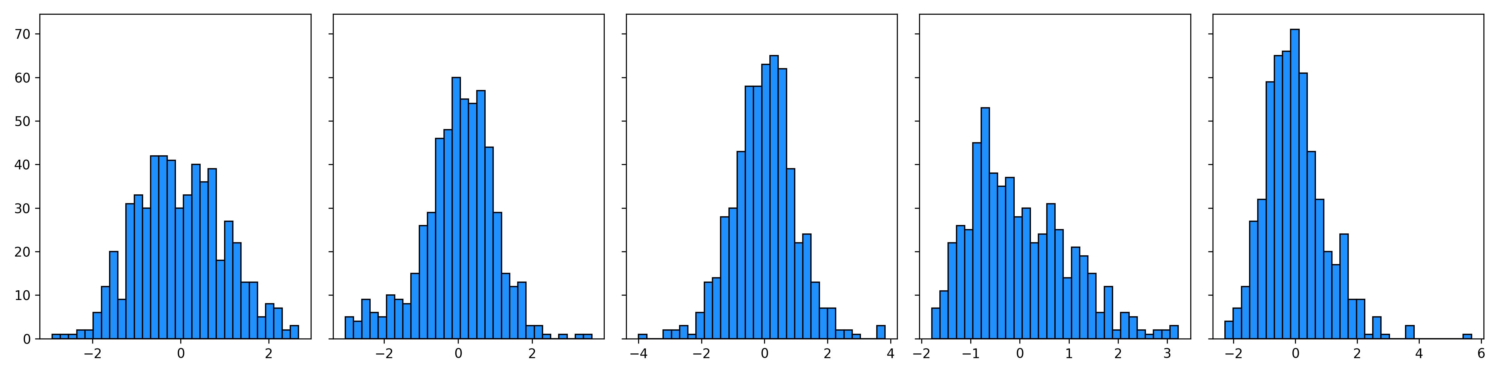
Figure 2. Distributions of five genes from the RNA-seq dataset.

4.1.  Simulation details.

Algorithm S2 describes the simulation procedure, which is also illustrated in Figure 1. In all steps, “randomly select” means select a parameter uniformly at random from its domain. The general outline is as follows: First, randomly select an $n$-by-$p$ submatrix $X$ of the full RNA-seq dataset and standardize its columns to have mean 0 and variance 1. Next, randomly select a true subset of $p_{\mathrm{true}}$ important features $S$, and partition it into $G$ groups, $S_{1},\dots,S_{G}$. A different realization of a randomized nonlinear function $f_{\theta_{g}}$, defined in Equation S2.1, is applied to the standardized sum $\xi_{g}=(\hat{\xi}_{g}-\bar{\xi}_{g})/\bar{\sigma}_{g}$ of the features in each group $S_{g}$, where $\bar{\xi}_{g}$ and $\bar{\sigma}_{g}$ are the empirical mean and standard deviation of $\hat{\xi}_{g}=\sum_{j\in S_{g}}X_{j}$. The resulting values are summed over all groups to generate a signal $\eta=\sum_{g=1}^{G}f_{\theta_{g}}(\xi_{g})$, and noise is added to this signal to generate a response $y$. This scheme produces data with highly complex interactions between features and the response, going well beyond the additive setting $y=\sum_{j\in S}f_{j}(X_{j})+\epsilon$.

Regression and classification data are simulated with $p=500$, $2000$, and $5000$ features for a total of six experiments. Each experiment consists of $100$ trials, outlined in Algorithm S2. Each trial uses $n=500$ samples and $\lvert S\rvert=p_{\mathrm{true}}$ important features. For regression, the response is $y=\sum_{g=1}^{G}f_{\theta}(\xi_{g})+\epsilon$, where $\epsilon\sim\mathcal{N}(0,\sigma^{2}I)$ and the variance $\sigma^{2}$ is selected according to a specified signal-to-noise ratio (SNR). For classification, we draw $y_{i}\sim\mathrm{Bernoulli}(\pi_{i})$ where $\pi_{i}=1/(1+\exp(-u\eta_{i}))$. A new $p_{\mathrm{true}}$ and SNR (or $u$), as well as new sets of samples, features, and important features, are drawn prior to each trial, with $p_{\mathrm{true}}$, SNR, and $u$ chosen according to Table S1. The many sources of randomness in our setup are introduced so that the simulations cover a wide range of settings.

4.2.  Simulation results.

Figures 3, LABEL:, 4, LABEL:, and 5 show the results. The empirical false discovery and true positive rates are $\mathrm{FDR}=\mathrm{FP}/(\mathrm{TP}+\mathrm{FP})$ and $\mathrm{TPR}=\mathrm{TP}/(\mathrm{TP}+\mathrm{FN})$, where FP, TP, and FN are the number of false positives, true positives, and false negatives, respectively. The upper left (high TP or TPR and low FP or FDR) corresponds to better performance in Figures 3 and 4. The ability of the different methods to control E(FP) (Figure 3) and FDR (Figure 4) at their target values is shown when applicable. Specifically, SSBoost and KOBT provide theoretical control of E(FP) and FDR, respectively, while the IPSS methods can be specified to control either E(FP) or FDR (Section 2.2). In Figure 3, the dashed vertical line signifies a target E(FP) of 3, with ✖ symbols showing the average FP and TP for the relevant methods at this target value. In particular, the ✖ for a method with perfect E(FP) control should lie on the dashed vertical line. Similarly, the ✖ and ★ symbols in Figure 4 correspond to target FDRs of 0.1 and 0.3, respectively.

IPSSGB has the best performance overall. Its curves are the farthest to the upper left in every plot in Figures 3 and 4, and it has the best control of both E(FP) and FDR. In Figure 3, for example, the ✖ for IPSSGB is the closest to the vertical dashed line in all experiments, and similarly in Figure 4. Furthermore, IPSSGB identifies the most true positives, both in terms of average TP and average TPR. Notably, at a target E(FP) of 3 and a target FDR of 0.3, IPSSGB has the largest average TP and highest TPR in nearly every setting, while having significantly fewer false positives than most other methods. Figure 5 also shows that IPSSGB is one of the fastest methods, running in under 20 seconds in all settings.

Among the other methods with theoretical error control, IPSSRF performs well in terms of identifying true positives while controlling false positives, though not as well as IPSSGB. IPSSL, whose model assumptions are violated, performs poorly, neither controlling false positives at the target E(FP) or FDR levels, nor identifying many true ones. SSBoost, whose curves are obtained by varying the target E(FP) between 0 and 10, has few false positives but also few true positives. Observe, for example, that the ✖ for SSBoost in Figure 3 is always significantly lower than those for IPSSGB and IPSSRF, despite all three methods having the same target E(FP). This is due in part to the weakness of the efp scores used by SSBoost relative to those used by IPSS (Melikechi and Miller, 2024). KOBT performs poorly in general; most notably, its actual FDRs far exceed its target FDRs of 0.1 and 0.3 in all of the simulation settings in Figure 4. KOBT also runs in around 90 seconds, making it one of the slowest methods. With the exception of IPSSL for classification, all of the stability selection-based methods run in at most 40 seconds, often less.

The absence of error control for Boruta and Vita is clearly apparent in Figures 3 and 4. Both methods usually have FDRs over 0.75—often 20 or more false positives on average—far surpassing IPSSGB and IPSSRF. Despite this, Boruta and Vita identify fewer true positives than IPSSGB with a target E(FP) of 3 and, in many cases, IPSSGB with a target FDR of 0.3. The RF and XGBoost curves are obtained by increasing the number of features selected, as ranked by their importance scores, from 0 to 30; that is, the first nonzero point along the curve is obtained by keeping only the feature with the highest importance score, the second point is obtained by keeping the features with the two largest importance scores, and so on. Interestingly, RF and XGBoost significantly underperform IPSSGB and IPSSRF in terms of true and false positives across the whole 0 to 30 range, indicating that IPSS is able to identify important features that simple thresholding of the baseline algorithm cannot, no matter how many features are kept. In terms of runtime, RF and XGBoost run quickly except in the $p=5000$ regression experiment. Boruta and Vita are typically slower than the IPSS methods, and this disparity grows with the number of features.

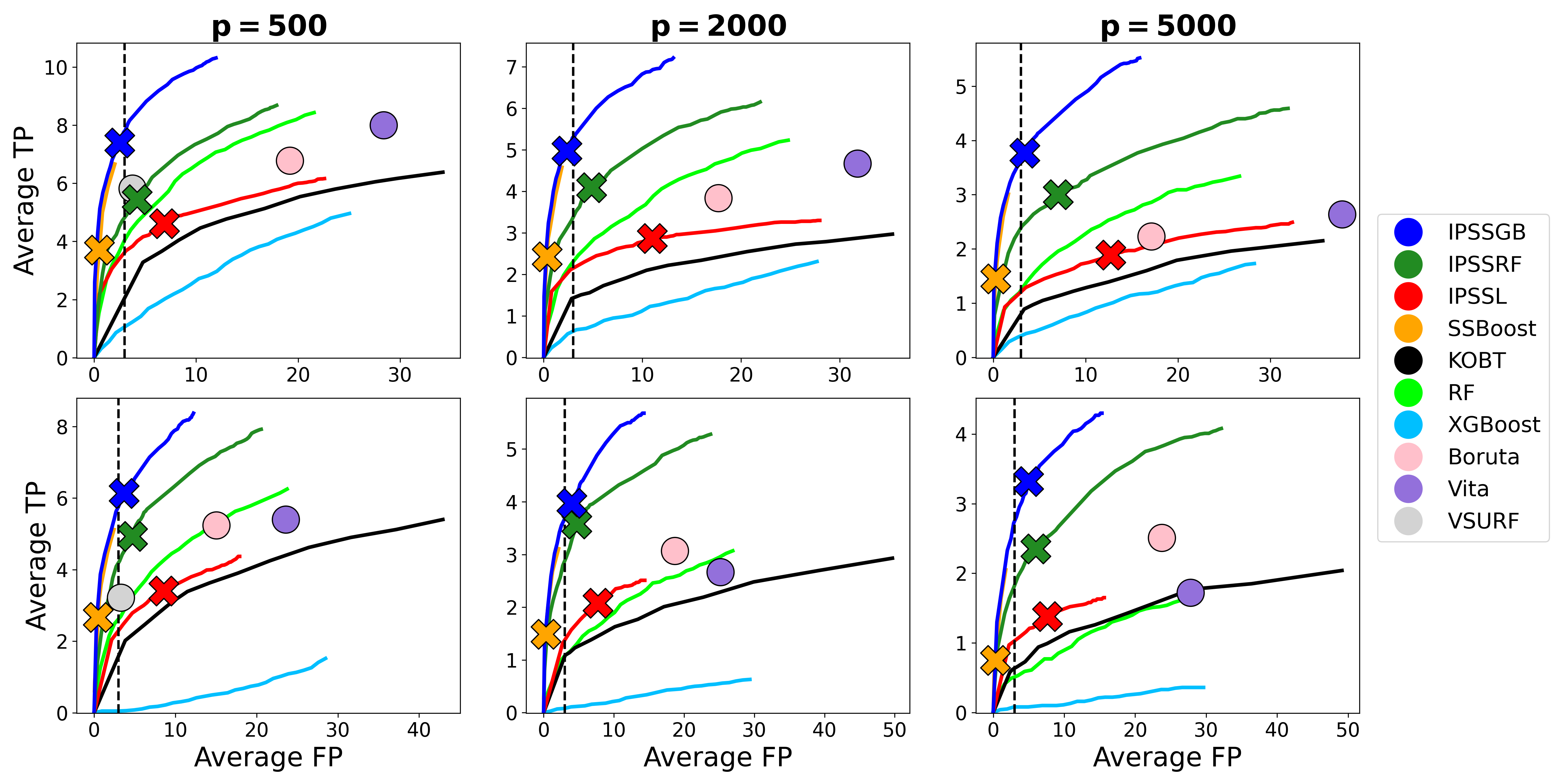
Figure 3. TP versus FP for the six simulation experiments. Columns correspond to the number of features, $p$, and the top and bottom rows correspond to regression and classification, respectively. Curves for the three IPSS methods and SSBoost are obtained by varying the target E(FP), with ✖ showing results when the target E(FP) is 3. The KOBT curve is obtained by varying the target FDR, and the RF and XGBoost curves are obtained by increasing the number of features selected (as ranked by their importance scores) from 0 to 30. The remaining methods, indicated by the ⚫ symbols, do not have curves because they select fixed sets of features.

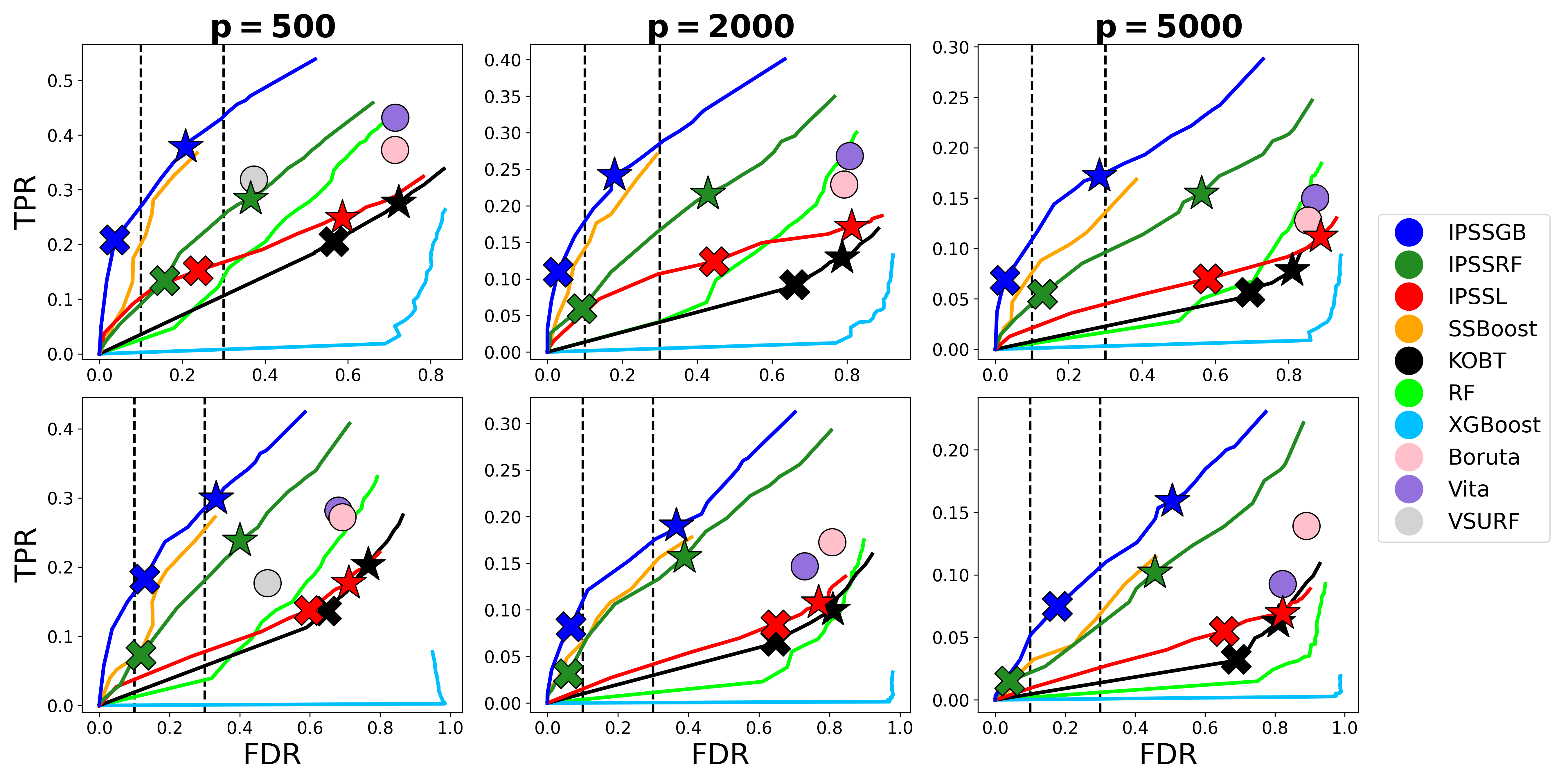
Figure 4. TPR versus FDR for the six simulation experiments. Results are similar to those in Figure 3, except now we show the FDR and TPR rather than E(FP) and E(TP), and curves for the three IPSS methods and KOBT are obtained by varying the target FDR, with ✖ and ★ showing results when the target FDR is 0.1 and 0.3.

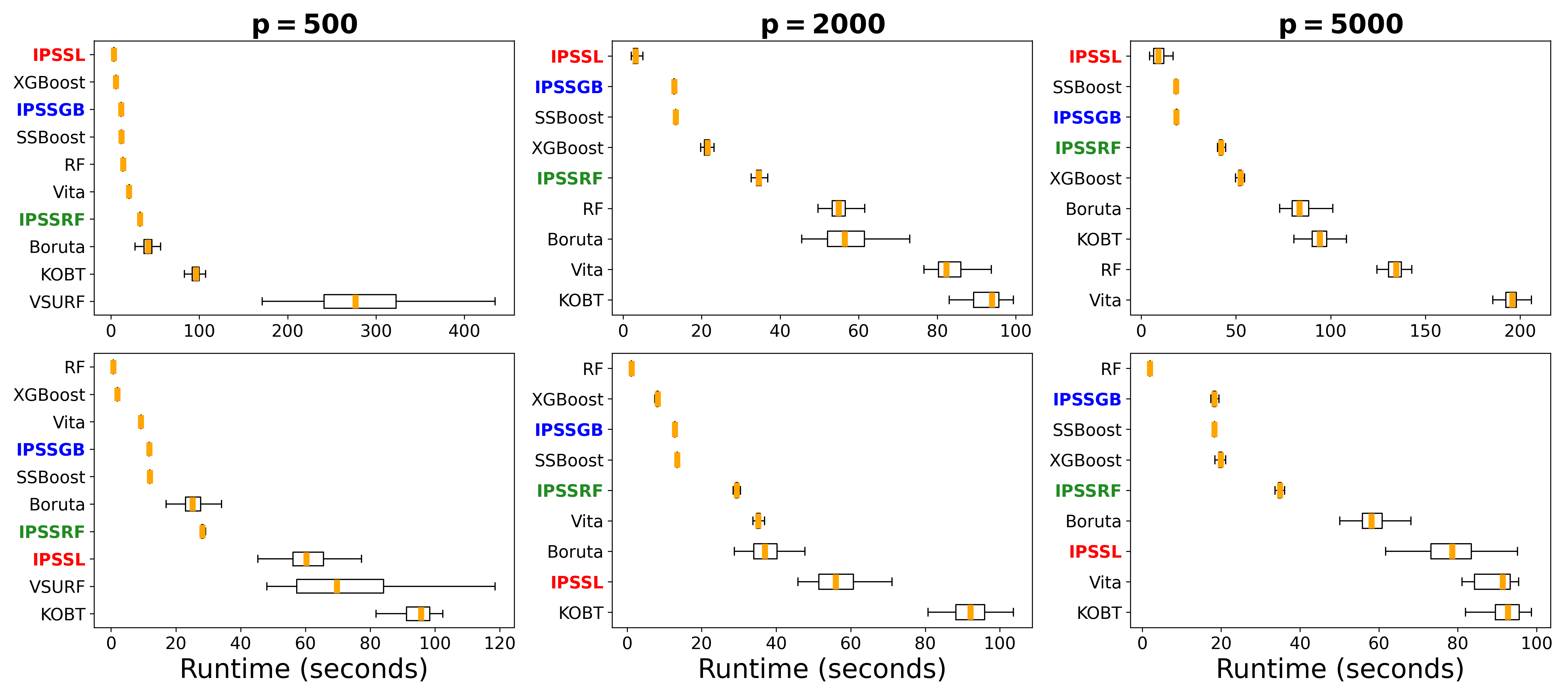
Figure 5. Runtimes for the six experiments. Columns correspond to the number of features, $p$, and the top and bottom rows correspond to regression and classification, respectively. Orange lines denote median runtime and whiskers extend to 1.5 times the interquartile range.

5.  Ovarian cancer

We apply IPSSGB, IPSSRF, and the other methods in Table 1 to microRNA (miRNA) data from the cohort of ovarian cancer patients described in Section 4 (Vasaikar et al., 2018). We report two studies here; see Section S3 for results from additional studies, including analyses of the RNA-seq data from this cohort. In the first study, the features are the 588 miRNAs and the response variable is prognosis, which is defined as whether the patient was still alive at the time of last follow-up. In the second study, the response is one of the miRNAs, miR-150, identified as important in the first stage, and the features are the remaining miRNAs. Thus, since miRNA measurements are continuous, the first study is a binary classification problem, and the second study is regression.

All analyses, both here and in Section S3, are conducted using 10-fold cross-validation (CV) as follows. First, all patients with missing values are removed, resulting in $n=442$ and $n=453$ for the first and second studies, respectively. The remaining patients are evenly partitioned into 10 groups. In each of the 10 CV steps and for each selection method, one group of patients is set aside (the test set), and a set of miRNAs is selected by applying the method to the data in the remaining groups (the training set). For the IPSS methods, we also compute the efp scores and $q$-values of each miRNA on the training set. Next, for each method we construct three predictive models—a linear model (either lasso or $\ell^{1}$-regularized logistic regression), a random forest model, and a gradient boosting model—using only the miRNAs selected by that method. Each model is then used to predict responses from the test set, and the smallest of the three prediction errors is recorded. We implement all three models so that no method has an inherent advantage over another. For example, the miRNAs selected by IPSSL may be better suited to minimizing error in a linear model than those selected by IPSSGB, while the miRNAs selected by IPSSGB may be better suited to minimizing error in a gradient boosting model than those selected by IPSSL. The linear and random forest predictive models are implemented with scikit-learn (Pedregosa et al., 2011) and gradient boosting with XGBoost (Chen and Guestrin, 2016), always with default parameters. For continuous responses, in each CV step we subtract the mean of the training responses from all responses, training and test, and scale all responses by the empirical standard deviation of the training responses.

Table 2 shows the top five miRNAs related to prognosis for each IPSS method, as ranked by their median $q$-values over the 10 CV steps. In Section S3, we further investigate the findings in Table 2 via a literature review. Notably, we find numerous studies that link several of the top miRNAs selected by IPSSGB and IPSSRF, namely miR-30d, miR-93, miR-96 and miR-150, to ovarian cancer prognosis. Among these, IPSSL only ranks miR-96 in its top five, and we found little literature identifying its top-ranked feature, miR-1-2, to ovarian cancer. The results of the second study, identifying miRNAs that are related to miR-150, are shown in Figure 6. Here, IPSSGB achieves the lowest average prediction error over the 10 cross-validation steps of any method, while using just 15 to 20 miRNAs, achieving lower prediction error than even the method that uses all 587 miRNAs to predict miR-150 levels (the dashed gray line in Figure 6). Figure 7 is similar to Figure 6, except now the response is tumor purity, the proportion of cancerous cells in a tissue sample. Here, we see IPSSGB performs best with the fewest features, while the top 30 features selected by IPSSRF achieve essentially identical predictive performance to the method that uses all 588 miRNAs.

IPSSGB	IPSSRF	IPSSL
miR-96(0.2)	miR-1270(0.27)	miR-1-2(0.07)
miR-150(0.28)	miR-93(0.36)	miR-1270(0.08)
miR-1270(0.43)	miR-30d(0.36)	miR-96(0.09)
miR-30d(0.43)	miR-342(0.36)	miR-342(0.09)
miR-1301(0.46)	miR-150(0.41)	miR-934(0.12)

Table 2. MicroRNA and prognosis. The top five miRNAs related to prognosis according to each IPSS method, as ranked by their median $q$-values over the 10 cross-validation steps.

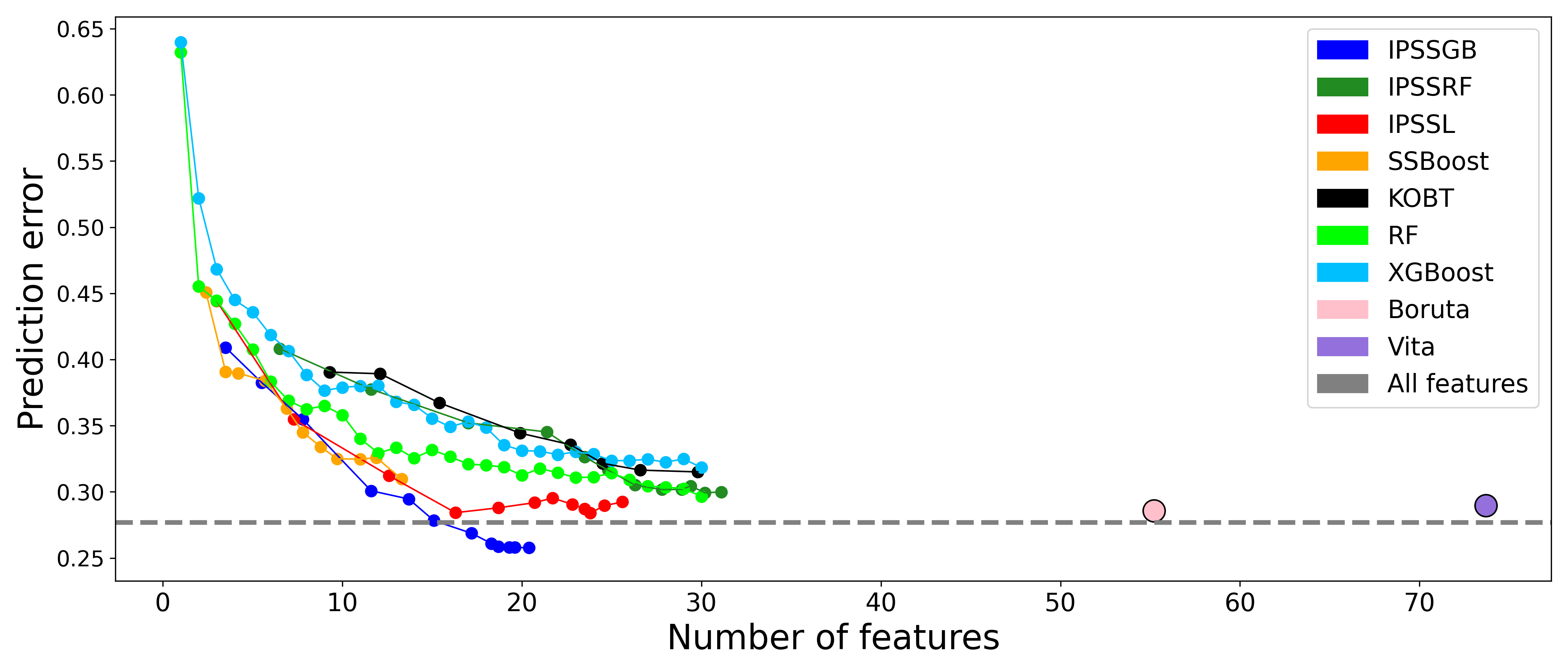
Figure 6. MicroRNA and miR-150. The horizontal and vertical axes show the average number of features selected and the average prediction error over the 10 cross-validation steps, respectively. Curves for the IPSS methods and SSBoost are obtained by varying the target E(FP) between 1/8 and 10. Points for these methods correspond to target E(FP)s of 1/8, 1/4, 1/2, 1, 2, 3, 4, 5, 6, 7, 8, 9, 10, with larger target E(FP)s generally corresponding to more features selected and lower prediction error. Similarly, points for KOBT correspond to target FDRs of 0.01, 0.025, 0.05, 0.1, 0.15, 0.2, 0.25, 0.3, and 0.4. The points for RF and XGBoost correspond to selecting between 1 and 30 features (hence, the number of features selected by these two methods is deterministic). Boruta and Vita do not have error control parameters and are therefore indicated by single points rather than curves.

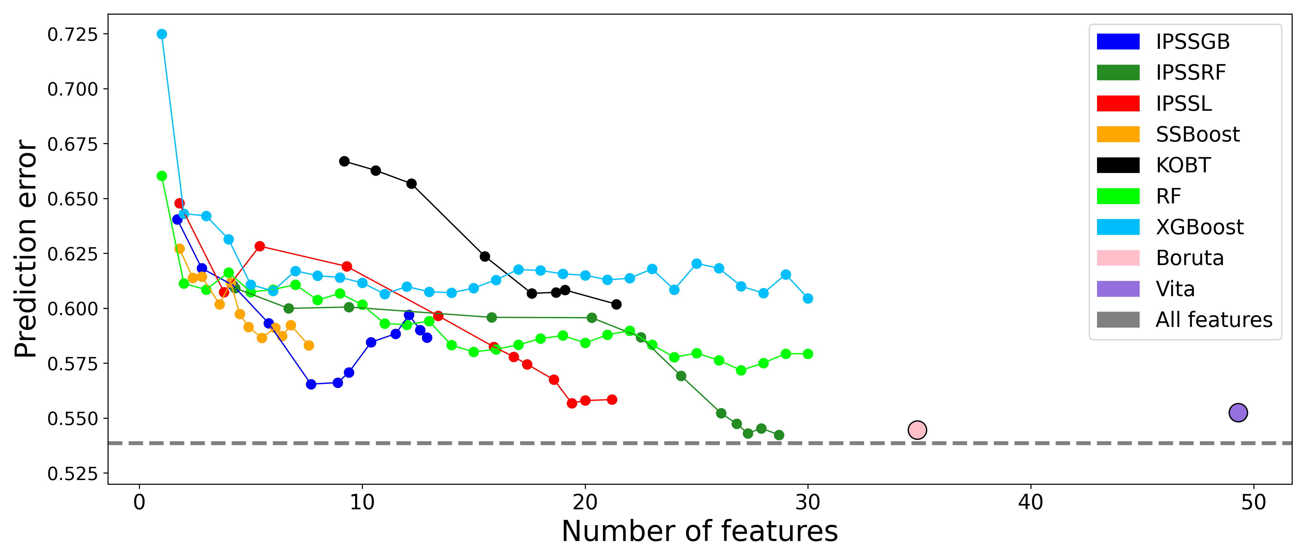
Figure 7. MicroRNA and tumor purity. This is the same as Figure 6, except now the response is tumor purity, the proportion of cancerous cells in a sample. We again see the IPSS methods outperform other methods, achieving similar or better predictive performance with relatively few features.

6.  Discussion

We have demonstrated that IPSSRF and IPSSGB achieve superior results in terms of false positive control, detecting true positives, and computation time. More broadly, IPSS for thresholding is a general framework whose theory and implementation apply to arbitrary importance scores. For instance, examples of other scores include $p$-values (with smaller $p$-values indicating greater importance), Shapley values (used to quantify the contribution of individual features to neural networks and other machine learning models), and loadings in principal components analysis (which quantify the contribution of each feature to a given principal component). The main practical limitation to consider is the cost of computing the relevant importance scores, since IPSS must compute these scores on many random subsamples of the data.

We have also introduced efp scores and shown that, in addition to controlling E(FP), they can control the FDR and estimate $q$-values. Storey (2003) showed that $q$-values admit a Bayesian interpretation, suggesting a link between IPSS and Bayesian feature selection that could be an interesting line of future work. It would also be interesting to study whether $q$-values estimated from efp scores are more accurate than $q$-values estimated from other quantities, such as $p$-values (Storey and Tibshirani, 2003).

Finally, a more ambitious goal is to extend IPSS to unsupervised feature selection problems (that is, feature selection when there is no response variable) and non-iid data. The PCA-based scores mentioned above provide at least one way to apply IPSS in an unsupervised setting. Developing a rigorous approach to IPSS for non-iid data could provide novel methods for nonparametric feature selection with error control for time series, networks, and longitudinal data.

Data availability and code

All of the code and data used in this work are freely available at https://github.com/omelikechi/ipss. A Python package for implementing integrated path stability selection, including IPSSGB and IPSSRF, is freely available at https://pypi.org/project/ipss/

S1.  Additional IPSS details

We provide an algorithm that implements integrated path stability selection (IPSS) for thresholding (Section S1.1), elaborate on the theory of IPSS and its connection to efp scores (Section S1.2), and describe and study the IPSS parameters in greater detail (Section S1.3).

S1.1.  Algorithm.

Algorithm S1, discussed in Section 2.3, implements IPSS for thresholding. The number of grid points used to evaluate the integrals in Algorithm S1 is always $K=100$. Like many of the other IPSS parameters, $K$ is inconsequential provided it is sufficiently large; in our experience, values greater than 25 suffice. This is because the function $f(x)=(2x-1)^{3}\operatorname{\mathds{1}}(x\geq 0.5)$, the paths $\lambda\mapsto\hat{\pi}_{j}(\lambda)$ (which are monotonically increasing functions of $\lambda$), the quantity $\mathcal{I}(\Lambda)$, and the measure $\mu$ are all very numerically stable.

Algorithm S1 Integrated path stability selection for thresholding

1:Data $Z_{1:n}$, importance function $\Phi$, number of grid points $K$, and number of iterations $B$.

2:(Optional) Preselect features, as described in Section S1.4.

3:for $b=1,\ldots,B$ do

4:     Randomly select $A_{2b-1},A_{2b}\subseteq\{1,\ldots,n\}$ with $A_{2b-1}\cap A_{2b}=\varnothing$ and $\lvert A_{2b-1}\rvert=\lvert A_{2b}\rvert=\lfloor n/2\rfloor$.

5:     Evaluate $\Phi_{Z_{A_{2b-1}}}(j)$ and $\Phi_{Z_{A_{2b}}}(j)$ for $j=1,\dots,p$.

6:end for

7: Set $\lambda_{\mathrm{max}}=\max\{\Phi_{Z_{A_{b}}}(j):1\leq b\leq 2B,\,1\leq j\leq p\}$.

8:Define a $\lambda$ grid with upper bound $\lambda_{\mathrm{max}}$, e.g., $\lambda_{\mathrm{max}}=\lambda_{0}>\lambda_{1}>\cdots>\lambda_{K}=\lambda_{\mathrm{max}}/10^{8}$.

9:Initialize $\lambda_{\mathrm{min}}\leftarrow\lambda_{\mathrm{max}}$ and $k\leftarrow 0$.

10:while $\mathcal{I}([\lambda_{\mathrm{min}},\lambda_{\mathrm{max}}])<0.05$ do

11:     $\hat{S}_{\lambda}(Z_{A_{b}})=\{j:\Phi_{Z_{A_{b}}}(j)\geq\lambda\}$ for $b=1,\dots,2B$.

12:     $\lambda_{\mathrm{min}}\leftarrow\lambda_{k+1}$ followed by $k\leftarrow k+1$.

13:end while

14:$\Lambda\leftarrow[\lambda_{\mathrm{min}},\lambda_{\mathrm{max}}]$.

15:Evaluate estimated selection probability $\hat{\pi}_{j}(\lambda)=\frac{1}{2B}\sum_{b=1}^{2B}\operatorname{\mathds{1}}\!\big{(}j\in\hat{S}_{\lambda}(Z_{A_{b}})\big{)}$ for $j=1,\dots,p$.

16:Evaluate the integral ${\int}_{\Lambda}f(\hat{\pi}_{j}(\lambda))\mu(d\lambda)$ for $j=1,\dots,p$.

17:$\mathtt{efp}_{Z_{1:n}}(j)=\mathcal{I}(\Lambda)/{\int}_{\Lambda}f(\hat{\pi}_{j}(\lambda))\mu(d\lambda)$ for $j=1,\dots,p$.

S1.2.  Theory: From IPSS to efp scores.

Given the estimated selection probabilities $\hat{\pi}_{j}$, an interval $\Lambda\subseteq(0,\infty)$, a probability measure $\mu$ on $\Lambda$, a function $f:[0,1]\to\mathbb{R}$, and a threshold $\tau$, Melikechi and Miller (2024) define the set of features selected by IPSS by

$$\hat{S}_{\mathrm{IPSS}}(\tau) =\Big{\{}j:{\int}_{\Lambda}f(\hat{\pi}_{j}(\lambda))\mu(d\lambda)\geq\tau\Big{\}}.$$ (S1.1)

The integral incorporates information about the selection probabilities over all of $\Lambda$, eliminating the need to select features based on individual $\lambda$ values. The function $f$ transforms the selection probabilities for better performance. Only certain choices of $f$ are known to yield valid efp scores. Melikechi and Miller (2024) prove the following result (see Theorem 4.1 therein). Let $q(\lambda)=\mathrm{E}\lvert\hat{S}_{\lambda}(Z_{1:\lfloor n/2\rfloor})\rvert$ be the expected number of features selected by $\hat{S}_{\lambda}$ on half the data and, for $m\in\mathbb{N}$, define $h_{m}(x)=(2x-1)^{m}\operatorname{\mathds{1}}(x\geq 0.5)$. For any $\Lambda$ and $\mu$, if

$$\max_{j\in S^{c}}\,\mathbb{P}\bigg{(}j\in\bigcap_{b=1}^{m^{\prime}}\big{(}\hat{S}_{\lambda}(Z_{A_{2b-1}})\cap\hat{S}_{\lambda}(Z_{A_{2b}})\big{)}\bigg{)} \leq(q(\lambda)/p)^{2m^{\prime}},$$ (S1.2)

for all $\lambda\in\Lambda$ and $m^{\prime}\in\{1,\dots,m\}$, then IPSS with $f=h_{m}$ satisfies

$$\mathrm{E}\lvert\hat{S}_{\mathrm{IPSS}}(\tau)\cap S^{c}\rvert \leq\frac{\mathcal{I}_{m}(\Lambda)}{\tau}$$ (S1.3)

for a constant $\mathcal{I}_{m}(\Lambda)$ whose explicit form is given in Theorem 4.1 in Melikechi and Miller (2024). Thus, setting $\mathtt{efp}_{Z_{1:n}}(j)=\mathcal{I}_{m}(\Lambda)/\int_{\Lambda}h_{m}(\hat{\pi}_{j}(\lambda))\mu(d\lambda)$ and $\hat{S}(t)=\{j:\mathtt{efp}_{Z_{1:n}}(j)\leq t\}$, we have

$$\hat{S}(t) =\bigg{\{}j:\frac{\mathcal{I}_{m}(\Lambda)}{\int_{\Lambda}h_{m}(\hat{\pi}_{j}(\lambda))\mu(d\lambda)}\leq t\bigg{\}}=\bigg{\{}j:{\int}_{\Lambda}h_{m}(\hat{\pi}_{j}(\lambda))\mu(d\lambda)\geq\frac{\mathcal{I}_{m}(\Lambda)}{t}\bigg{\}}=\hat{S}_{\mathrm{IPSS}}\bigg{(}\frac{\mathcal{I}_{m}(\Lambda)}{t}\bigg{)}$$

and hence

$$\mathrm{E}(\mathrm{FP}(t)) =\mathrm{E}\lvert\hat{S}(t)\cap S^{c}\rvert=\mathrm{E}\big{\lvert}\hat{S}_{\mathrm{IPSS}}\big{(}\tfrac{\mathcal{I}_{m}(\Lambda)}{t}\big{)}\cap S^{c}\big{\rvert}\leq t,$$

where the inequality holds by Equation S1.3.

The above derivation shows how valid efp scores for IPSS with $f=h_{m}$ are obtained under the conditions of Theorem 4.1 in Melikechi and Miller (2024). In particular, we see that by defining efp scores as above, the set $\hat{S}(t)=\{j:\mathtt{efp}_{Z_{1:n}}(j)\leq t\}$ is identical to $\hat{S}_{\mathrm{IPSS}}(\tau)$ when $\tau=\mathcal{I}_{m}(\Lambda)/t$. The main condition of the theorem, Equation S1.2, upper bounds the maximum probability that an unimportant feature is simultaneously selected on both halves of the data, $Z_{A_{2b-1}}$ and $Z_{A_{2b}}$, in $m^{\prime}$ independent tries; see Melikechi and Miller (2024) for details. The following result, part of Theorem 4.2 in Melikechi and Miller (2024), gives the form of $\mathcal{I}_{3}(\Lambda)$, which corresponds to the function $f=h_{3}$ that is used for IPSS throughout the main text.

Theorem S1.1.

Let $\mu$ be a probability measure on $\Lambda\subseteq(0,\infty)$, let $\tau\in(0,1]$, and define $\hat{S}_{\mathrm{IPSS}}(\tau)$ as in Equation S1.1 with $f=h_{3}$. If Equation S1.2 holds for all $\lambda\in\Lambda$ and $m^{\prime}\in\{1,2,3\}$, then

$$\mathrm{E}(\mathrm{FP}(\tau)) \leq\frac{1}{\tau}\int_{\Lambda}\bigg{(}\frac{q(\lambda)^{2}}{B^{2}p}+\frac{3q(\lambda)^{4}}{Bp^{3}}+\frac{q(\lambda)^{6}}{p^{5}}\bigg{)}\mu(d\lambda),$$ (S1.4)

where $\mathrm{E}(\mathrm{FP}(\tau))=\mathrm{E}\lvert\hat{S}_{\mathrm{IPSS}}(\tau)\cap S^{c}\rvert$ is the expected number of false positives selected by IPSS.

For some intuition about the bound in Equation S1.4, observe that taking $B\to\infty$ yields $\mathrm{E}(\mathrm{FP}(\tau))\leq\tau^{-1}\int_{\Lambda}\big{(}q(\lambda)^{6}/p^{5}\big{)}\mu(d\lambda)$. In comparison, other versions of stability selection upper bound $\mathrm{E}(\mathrm{FP}(\tau))$ by $q(\lambda)^{2}/p$ (Meinshausen and Bühlmann, 2010; Shah and Samworth, 2013), which is orders of magnitude larger than $q(\lambda)^{6}/p^{5}$ when $q(\lambda)\ll p$, as is often the case for most values of $\lambda$ in $\Lambda$. This and the contribution of $B$ in the denominators in Equation S1.4 largely explain the strength of the IPSS bound in Theorem S1.1 relative to previous bounds, and hence the tightness of the efp scores of IPSS with $f=h_{3}$ relative to the efp scores of other versions of stability selection. Further theoretical and empirical comparisons between Equation S1.4 and other stability selection bounds are available in Melikechi and Miller (2024).

S1.3.  Parameters.

As noted above, the function $f(x)=(2x-1)^{3}\operatorname{\mathds{1}}(x\geq 0.5)$ used when implementing IPSS in the main text is determined by the availability and strength of the theoretical bound in Theorem S1.1. Similarly, the choice of $\lfloor n/2\rfloor$ samples used to construct the selection probabilities $\hat{\pi}_{j}(\lambda)$ are required for stability selection theorems (not just Theorem S1.1) to hold, and it is unclear how to adapt their proofs to accommodate other sample sizes. Thus, $f$ and $\lfloor n/2\rfloor$ are theoretical necessities rather than free parameters.

The interval $\Lambda=[\lambda_{\mathrm{min}},\lambda_{\mathrm{max}}]$ is determined by setting $\lambda_{\mathrm{max}}$ large enough that no features are selected (see, for example, 7 in Algorithm S1), and setting $\lambda_{\mathrm{min}}$ such that the integral

$$\mathcal{I}(\Lambda) =\int_{\Lambda}\bigg{(}\frac{q(\lambda)^{2}}{B^{2}p}+\frac{3q(\lambda)^{4}}{Bp^{3}}+\frac{q(\lambda)^{6}}{p^{5}}\bigg{)}\mu(d\lambda),$$

in Equation S1.4 is equal to a fixed cutoff $C$. As noted in the main text, we always use $C=0.05$, but results are largely independent of this choice (Figures S1 and S2). Figures S3 and S4 show IPSS is also indifferent to $\mu$. Here, the parameter $\delta$ determines the measure $\mu_{\delta}(d\lambda)=z_{\delta}^{-1}\lambda^{-\delta}d\lambda$, where the normalizing constant $z_{\delta}$ is easily computed in closed form (Melikechi and Miller, 2024). The probability measure that we always use in the main text, $\mu_{1}$, averages over $\Lambda$ on a log scale, while $\mu_{0}$ averages on a linear scale. The insignificance of $C$ and $\mu$ is unsurprising: Intuitively, the efp scores for IPSS depend primarily on $f$ and the integrand in $\mathcal{I}(\Lambda)$. The actual value of $\mathcal{I}(\Lambda)$ is much less important since the efp scores depend on the relative quantities $\mathcal{I}(\Lambda)/\int_{\Lambda}f(\hat{\pi}_{j}(\lambda))\mu(d\lambda)$ rather than on $\mathcal{I}(\Lambda)$ itself. Since $C$ and $\mu$ only affect the value of the bound, not the integrand, they contribute little to the actual performance of IPSS.

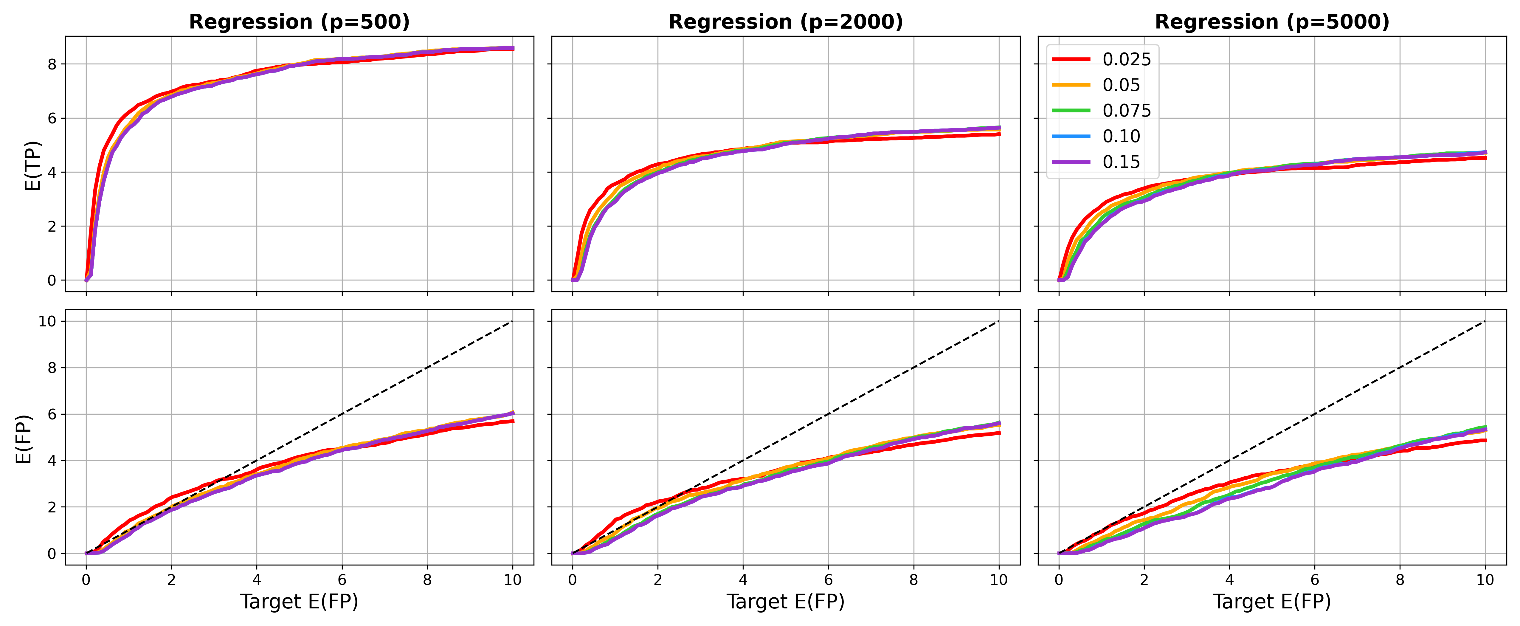
Figure S1. Dependence on cutoff (regression). IPSSGB is applied to regression data simulated as in Section 4 for cutoff values $C\in\{0.025,0.05,0.075,0.1,0.15\}$, averaged over 100 trials. There is little difference between the average true and false positive values for different choices of $C$ over a wide range of target E(FP) values. Figures S2, S3, and S4 show similar results for classification and dependence on $\mu$.

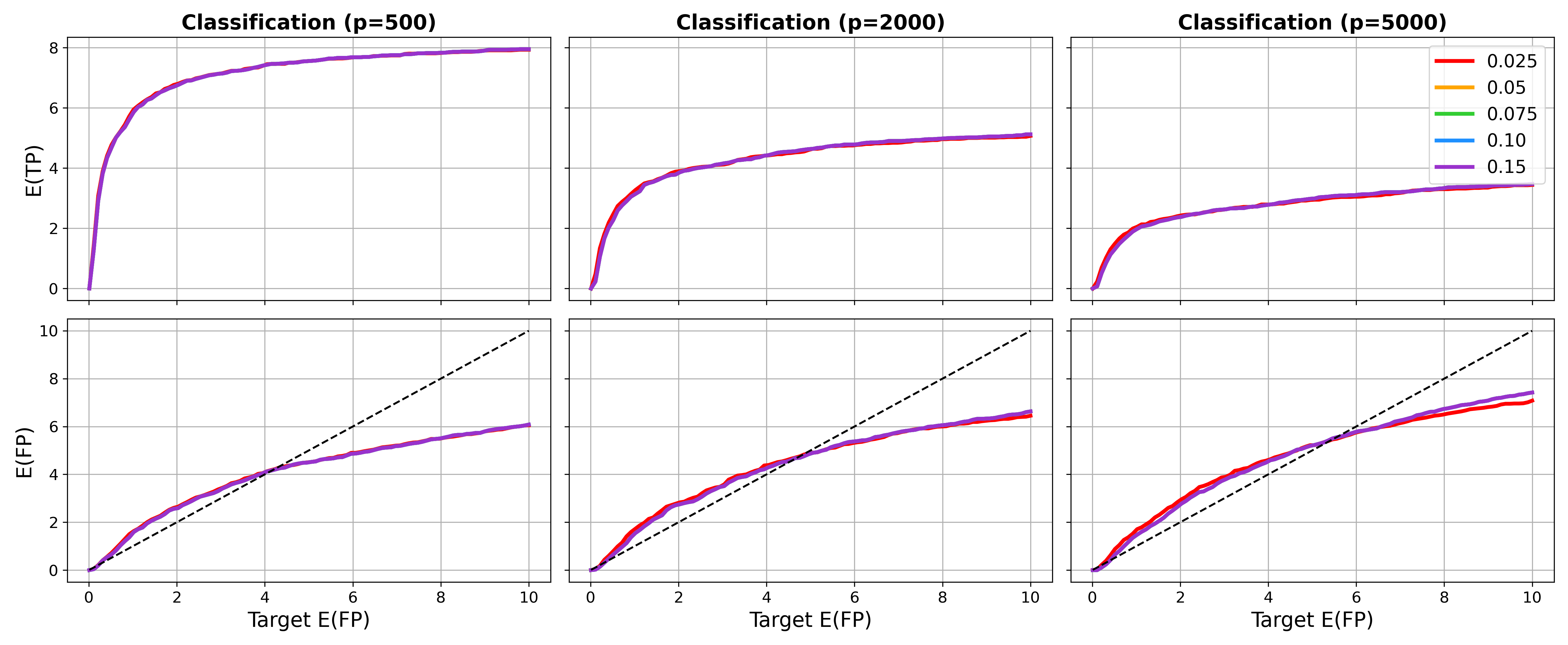
Figure S2. Dependence on cutoff (classification). IPSSGB is applied to classification data simulated as in Section 4 for cutoff values $C\in\{0.025,0.05,0.075,0.1,0.15\}$, averaged over 100 trials. There is little difference between the average true and false positive values for different choices of $C$ over a wide range of target E(FP) values.

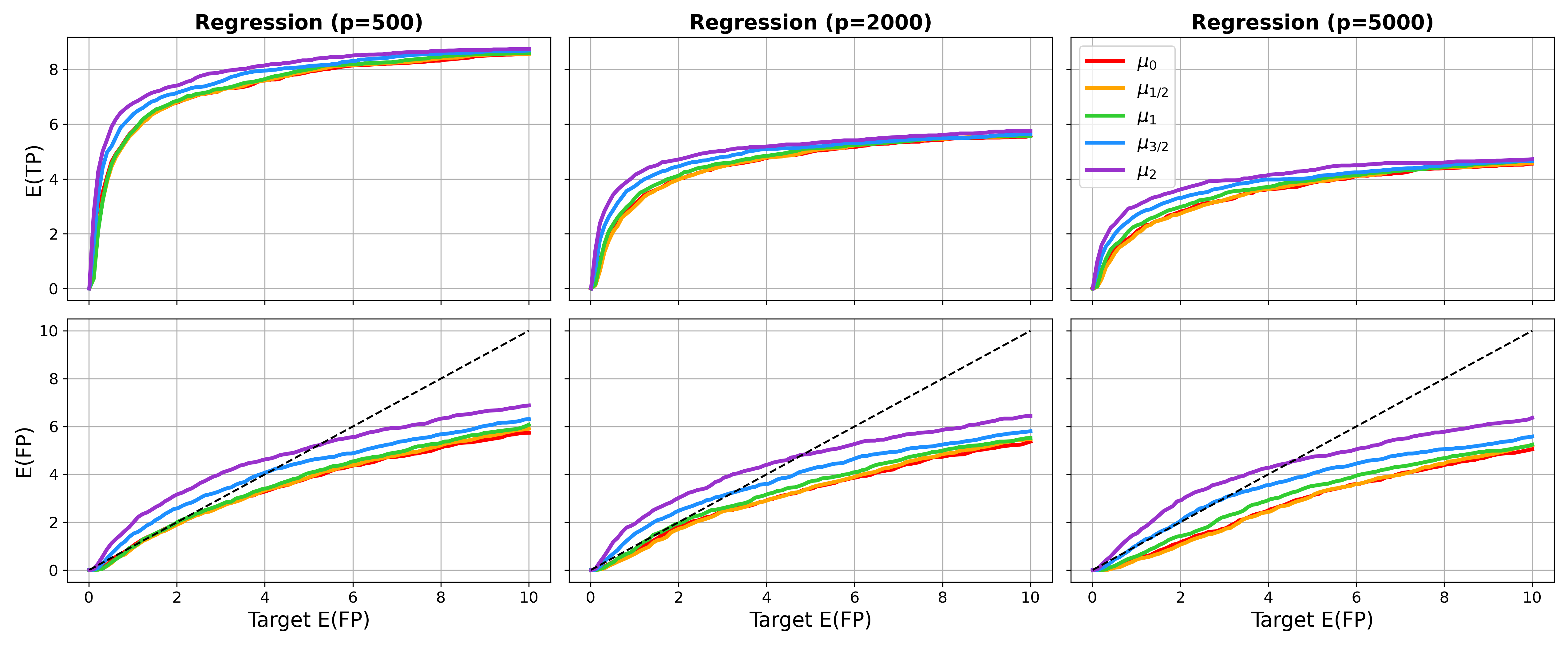
Figure S3. Dependence on $\mu$ (regression). IPSSGB is applied to regression data simulated as in Section 4 for cutoff values $\delta\in\{0,0.5,1,1.5,2\}$, averaged over 100 trials, where $\delta$ determines to the measure $\mu_{\delta}(d\lambda)=z_{\delta}^{-1}\lambda^{-\delta}d\lambda$. There is little difference between the average true and false positive values for different choices of $\delta$ over a wide range of target E(FP) values.

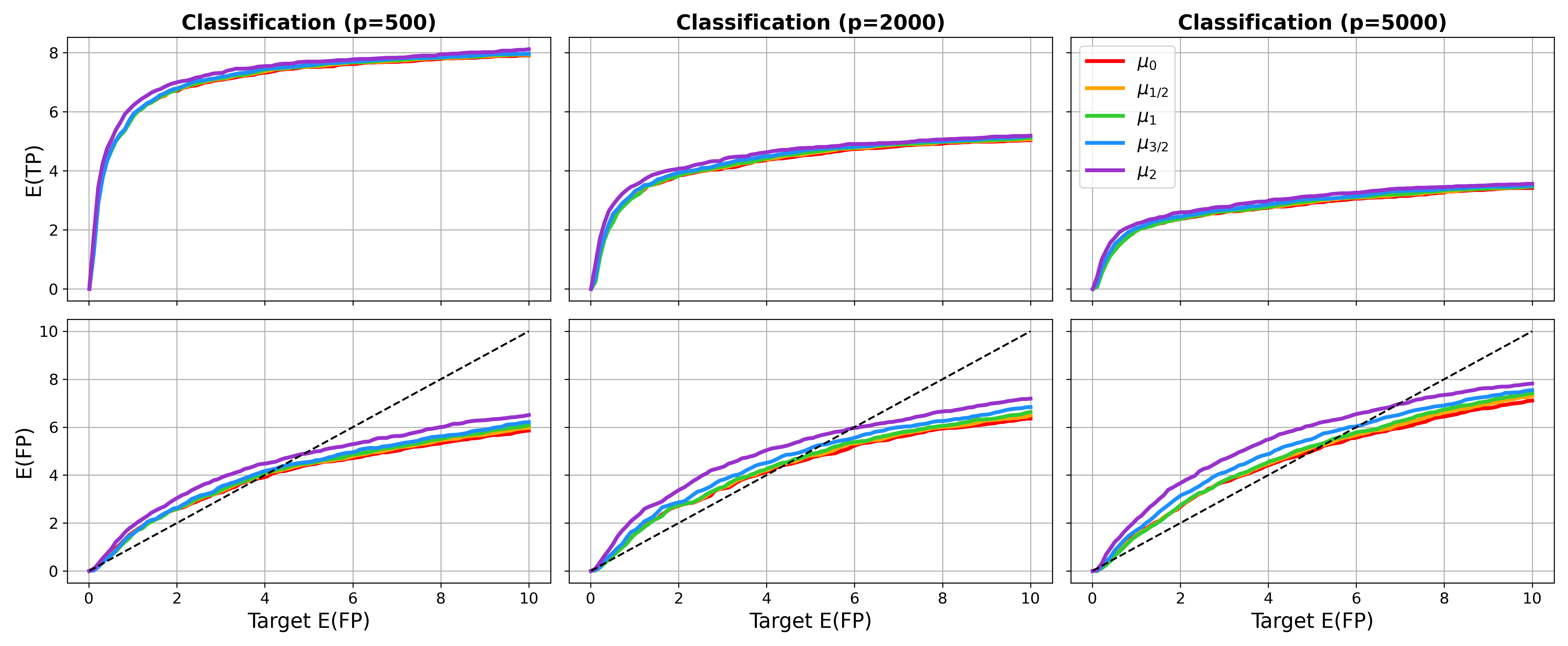
Figure S4. Dependence on $\mu$ (classification). IPSSGB is applied to classification data simulated as in Section 4 for cutoff values $\delta\in\{0,0.5,1,1.5,2\}$, averaged over 100 trials, where $\delta$ determines to the measure $\mu_{\delta}(d\lambda)=z_{\delta}^{-1}\lambda^{-\delta}d\lambda$. There is little difference between the average true and false positive values for different choices of $\delta$ over a wide range of target E(FP) values.

S1.4.  Preselection.

Many feature selection algorithms, including most in Section 3, employ some form of screening, or preselection, as an initial step in the selection process. This can be especially helpful in high dimensions for reducing noise and runtime. When $p>200$, we preselect features for IPSSGB, IPSSRF, and the other stability selection-based methods (IPSSL and SSBoost, detailed below) by running their respective selection algorithms on the full dataset three times—that is, computing $\Phi_{Z_{1:n}}$ three times—and keeping only the $p_{\text{pre}}=\max\{200,p/20\}$ features with the largest average scores across all three trials. Note that $\Phi_{Z_{1:n}}$ is stochastic, given $Z_{1:n}$, due to randomness in the gradient boosting and random forest algorithms. This preselection step does not affect the theoretical control on E(FP) since $\lvert\hat{S}_{\mathrm{IPSS},\mathrm{pre}}\cap S^{c}\rvert=\lvert\hat{S}_{\mathrm{IPSS},\mathrm{pre}}\cap S^{c}_{\mathrm{pre}}\rvert$, where $\hat{S}_{\mathrm{IPSS},\mathrm{pre}}$ are the features selected by IPSS using only the preselected features, and $S^{c}_{\mathrm{pre}}$ are the preselected features in $S^{c}$. Of course, preselection risks throwing away important features, potentially increasing the number of false negatives. However, we have yet to observe a case in which an important feature that was not in the top $p_{\mathrm{pre}}$ preselected features was selected by IPSS when the full set of features was used instead. In other words, a feature that does not make the top $p_{\mathrm{pre}}$ is highly unlikely to be selected by IPSS regardless of whether or not preselection is used.

S2.  Simulation details and additional results

Algorithm S2 describes the procedure we use to generate data in the simulation study in Section 4. See also Figure 1 in the main text for a diagrammatic representation of this process. In all steps, “randomly select” means select a parameter uniformly at random from its domain, which are shown in Table S1. The randomized function $f_{\theta}:\mathbb{R}\to[-1,1]$ that links the features to the response is

$$f_{\theta}(x) =\begin{cases}\frac{\delta_{1}}{2}\left(1+\tanh(\alpha(\delta_{2}x-\beta))\right)&\text{with probability}\ 1/2,\\ \delta_{1}\exp(-\gamma x^{2})&\text{with probability}\ 1/2,\end{cases}$$ (S2.1)

where each component of $\theta=(\alpha,\beta,\gamma,\delta_{1},\delta_{2})$ is drawn uniformly at random prior to each trial according to Table S1. The values of $\alpha$ and $\gamma$ determine steepness of the curves, $\beta$ shifts $\tanh$ horizontally, and $\delta_{1}$ and $\delta_{2}$ reflect the functions about the horizontal and vertical axes, respectively. Figure S7 shows five realizations of $f_{\theta}$, illustrating the many ways it can influence the response, $y$. For example, if the function in the left-most panel of Figure S7 is applied to the genes in a given partition of $S$, then those genes will only significantly affect $y$ if their collective expression level is positive, while collective expression levels less than $-1$ will have virtually no effect on $y$.

Parameter	$\alpha$	$\beta$	$\gamma$	$\delta_{1}$	$\delta_{2}$	$p_{\mathrm{true}}$	SNR	$u$
Range	$(0.5,1.5)$	$(-1,1)$	$(1,3)$	$\{-1,1\}$	$\{-1,1\}$	$\{10,\dots,30\}$	$(0.5,2)$	$(1,3)$

Table S1. Simulation parameters. Parameters are drawn uniformly at random from their corresponding ranges prior to each simulation trial.

Algorithm S2 Data generation for simulation study (one trial)

1:RNA-seq data $X_{\mathrm{full}}\in\mathbb{R}^{596\times 6426}$, number of samples $n$, number of features $p$, number of true features $p_{\mathrm{true}}$, signal-to-noise ratio SNR, function parameter domain $\Theta$.

2:Randomly select $n$ rows and $p$ columns of $X_{\mathrm{full}}$. Denote the resulting matrix by $X\in\mathbb{R}^{n\times p}$.

3:Standardize the columns of $X$ to have mean 0 and variance 1.

4:Randomly select true features $S\subseteq\{1,\dots,p\}$ with $\lvert S\rvert=p_{\mathrm{true}}$.

5:Randomly select $G\in\{\lfloor p_{\mathrm{true}}/2\rfloor,\dots,p_{\mathrm{true}}\}$. Partition $S$ into $G$ disjoint groups, $S=\bigsqcup_{g=1}^{G}S_{g}$.

6:Initialize the signal, $\eta\leftarrow(0,\ldots,0)^{\mathtt{T}}\in\mathbb{R}^{n}$.

7:for $g=1,\dots,G$ do

8:     $\xi_{g}\leftarrow\sum_{j\in S_{g}}X_{j}$ where $X_{j}\in\mathbb{R}^{n}$ is the $j$th column of $X$.

9:     Standardize $\xi_{g}$ to have mean 0 and variance 1.

10:     Randomly select a function parameter $\theta\in\Theta$.

11:     $\eta\leftarrow\eta+f_{\theta}(\xi_{g})$ with $f_{\theta}$ applied to $\xi_{g}\in\mathbb{R}^{n}$ componentwise.

12:end for

13:For regression: Draw $\epsilon_{i}\sim\mathcal{N}(0,\sigma^{2})$ with $\sigma^{2}=\sum_{i=1}^{n}\eta_{i}^{2}/(n\,\mathrm{SNR})$ and set $y_{i}\leftarrow\eta_{i}+\epsilon_{i}$.

14:For classification: Draw $u\sim\mathrm{Uniform}(1,3)$, then $y_{i}\sim\mathrm{Bernoulli}(\pi_{i})$ where $\pi_{i}=1/(1+\exp(-u\eta_{i}))$.

15:Features $X\in\mathbb{R}^{n\times p}$, responses $y\in\mathbb{R}^{n}$, and important features $S\subseteq\{1,\ldots,p\}$.

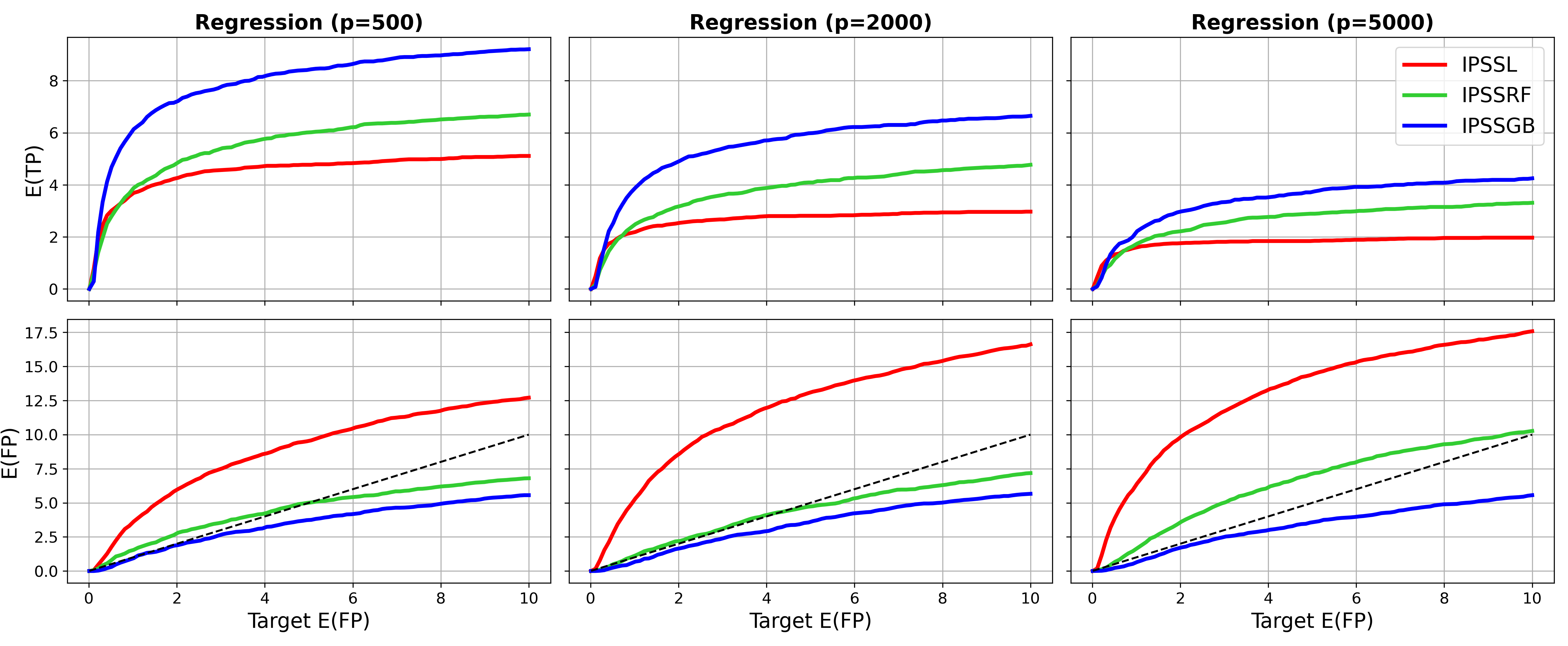
Figure S5. Regression simulation. Empirical E(FP) and E(TP) versus target E(FP) for each IPSS method. The dotted black line shows where E(FP) = target E(FP).

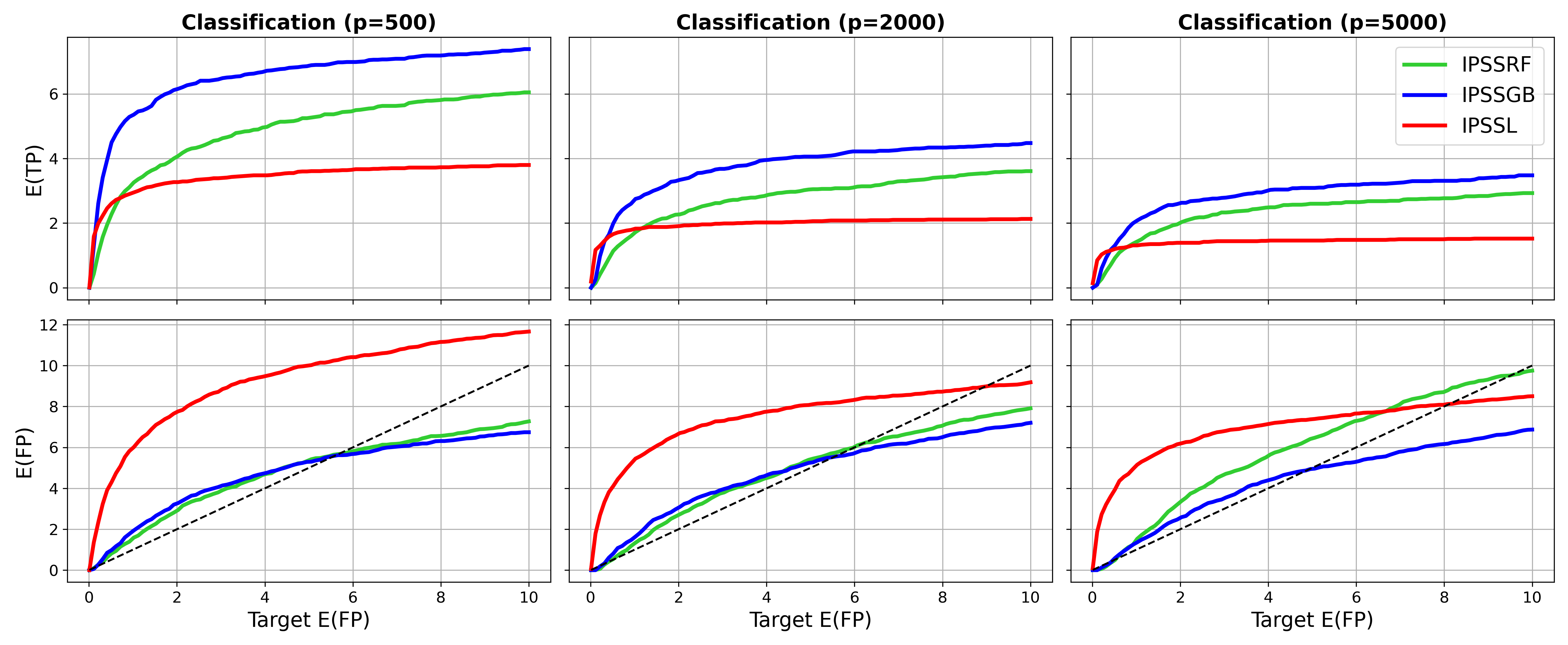
Figure S6. Classification simulation. Empirical E(FP) and E(TP) versus target E(FP) for each IPSS method. The dotted black line shows E(FP) = target E(FP).

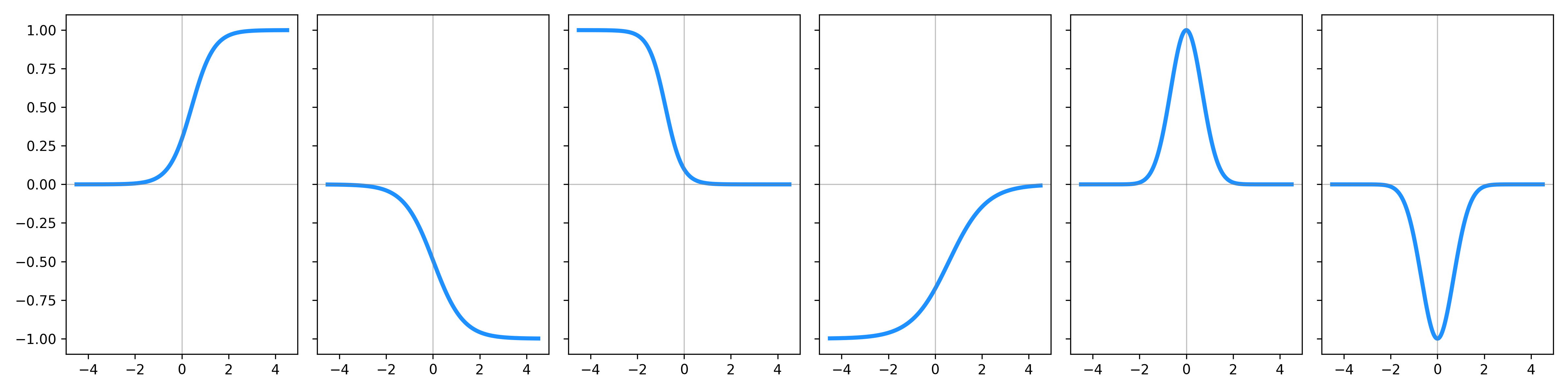
Figure S7. Some realizations of the randomized function $f_{\theta}$.

One benefit of IPSS is that changing the target E(FP) does not require rerunning the algorithm. Figures S5 and S6 show E(TP) and E(FP) as functions of the target E(FP). IPSSGB has the best performance in terms of true positives across essentially all target E(FP) values. IPSSGB and IPSSRF perform well in the regression setting, and both slightly overshoot the target E(FP) in classification for values less than 6. IPSSL performs poorly in general, having relatively few true positives on average and false positives that exceed the target E(FP).

S3.  Additional ovarian cancer results

In Section S3.1, we expand upon the ovarian cancer results presented in Section 5 of the main text, namely identifying miRNAs related to prognosis, and miRNAs related to miR-150, respectively. In Section S3.2, we perform a similar analysis but for RNA-seq data from the same cohort, identifying genes related to ovarian cancer prognosis, and genes related to one of the genes, AKT2, that was found to be related to prognosis.

S3.1.  MicroRNA and ovarian cancer.

We briefly summarize results from the literature that link the miRNAs in Table 2 to ovarian cancer, with a specific focus on prognosis. For many of these miRNAs, there are numerous studies connecting them to ovarian cancer beyond what we present. Thus, to roughly quantify the relevance of the miRNAs in Table 2 to ovarian cancer, we searched the specific miRNA together with “ovarian cancer” in the Web of Science database, and report both the number of publications and the total number of citations across all returned results. We emphasize that these metrics are less important than the papers themselves. For example, citation counts favor older publications, and our search criterion does not guarantee that the returned results are relevant to the problem at hand (though the summaries below show that at least some of them are).

Table S2 is similar to Table 2, except that it shows the total number of publications and citations from our Web of Science literature search and includes some $q$-values that were omitted from Table 2, since Table 2 only reported the five miRNA with the lowest $q$-values for each method. Dashed lines indicate that the feature was not identified by the corresponding method at all.

miRNA	Citations	Publications	IPSSGB	IPSSRF	IPSSL
miR-150	1635	26	0.28	0.41	0.2
miR-93	1270	28	–	0.36	–
miR-30d	596	12	0.43	0.36	0.16
miR-96	338	10	0.2	0.53	0.09
miR-342	201	9	–	0.36	0.09
miR-1270	175	5	0.43	0.27	0.08
miR-934	27	2	–	–	0.12
miR-1301	11	3	0.46	–	–
miR-1-2	5	1	–	–	0.07

Table S2. MicroRNA and prognosis. MiRNA are ordered by citations. A missing $q$-value means that miRNA was not selected by the corresponding version of IPSS.

miR-1-2. Kandettu et al. (2022) found that miR-1-2 is differentially expressed between cancerous and non-cancerous ovarian cancer cells, but we found no literature linking miR-1-2 to prognosis.

miR-30d. Ye et al. (2015) found that miR-30d suppresses ovarian cancer progression by reducing the levels of Snail, a protein involved in making cancer cells more invasive. They concluded that miR-30d could be used as a treatment for ovarian cancer. Lee et al. (2012) found that miR-30d is associated with “significantly better disease-free or overall survival” in ovarian cancer patients.

miR-93. Fu et al. (2012) found that miR-93 is significantly upregulated in ovarian cancer cells that are resistant to the chemotherapy drug cisplatin. They also found that miR-93 targets the tumor suppressor gene PTEN and plays a role in the AKT signaling pathway. They concluded that further study of miR-96 may yield therapeutic strategies for overcoming cisplatin-resistant ovarian cancer cells. Meng et al. (2015) found that miR-93 is a potential biomarker of ovarian cancer.

miR-96. Liu et al. (2019) found that overexpression of miR-96 promotes cell proliferation and migration in ovarian cancer cells. They conclude that targeting miR-96 is a potentially promising strategy for treating ovarian cancer. They also report that miR-96 inhibits phosphorylation of AKT, a gene identified by IPSSGB as being relevant to ovarian cancer prognosis (Section S3.2). Yang et al. (2020) found that individuals with low-levels of miR-96 “suffered more advanced tumor staging and a worse overall survival” and also identified miR-96 as a potential therapeutic target.

miR-150. Jin et al. (2014) found significant associations between miR-150 downregulation and “aggressive clinicopathological features” in ovarian cancer patients, as well as reduced overall and progression-free survival. They also identified miR-150 expression as a prognostic biomarker in ovarian cancer. Kim et al. (2017) found that downregulation of miR-150 is associated with resistance to paclitaxel, a chemotherapy drug used to treat ovarian cancer. They also report that treatment with pre-miR-150 resensitized cancer cells to paclitaxel, making the drug more effective.

miR-342. Dou et al. (2020) found that miR-342 inhibits the proliferation, invasion, and migration of ovarian cancer cells, and promotes the death of these cells. The study also showed that miR-342 decreases the expression of key proteins involved in the Wnt/$\beta$-catenin signaling pathway, which may explain its effects on reducing ovarian cancer cell viability and growth.

miR-934. Hu et al. (2019) found that miR-934 promotes ovarian cancer cell proliferation and inhibits the death of ovarian cancer cells by targeting the gene BRMS1L, making it is a potential biomarker or therapeutic target for ovarian cancer.

miR-1270. Ghafouri-Fard et al. (2022) found that miR-1270 plays a role in sensitivity to the chemotherapy drug cisplatin.

miR-1301. Yu and Gao (2020) found that targeting miR-1301 can inhibit the proliferation of cells that are resistant to the chemotherapy drug cisplatin, thus reducing the occurrence and development of drug-resistant ovarian cancer.

Tables S3 and S4 show the top ten features for each IPSS method, ranked by their median $q$-values over the 10 CV steps, when the features are miRNA and the responses are miR-150 (Table S3) and tumor purity (Table S4), respectively. Tumor purity is the proportion of cancerous cells in a sample. Observe that the $q$-values in Table S3 are much smaller than those in Table S2. This is to be expected since the signal between miRNAs, in particular, between miR-150 and certain other miRNAs, is likely much stronger than the signal between miRNAs and prognosis.

IPSSGB	IPSSRF	IPSSL
miR-142(0.031)	miR-146a(0.016)	miR-146a(0.028)
miR-146a(0.031)	miR-142(0.016)	miR-142(0.028)
miR-1247(0.031)	miR-223(0.016)	miR-1247(0.028)
miR-642(0.032)	miR-642(0.016)	miR-139(0.028)
miR-342(0.036)	miR-155(0.016)	miR-342(0.029)
miR-139(0.042)	miR-1247(0.016)	miR-642(0.029)
miR-1249(0.051)	miR-766(0.016)	miR-96(0.029)
miR-96(0.064)	miR-342(0.017)	miR-511-1(0.03)
miR-204(0.072)	miR-1228(0.018)	miR-34b(0.032)
miR-34b(0.074)	miR-21(0.02)	miR-184(0.033)

Table S3. MicroRNA and miR-150. Top ranked miRNAs for each method in terms of their $q$-values, shown in parentheses.

IPSSGB	IPSSRF	IPSSL
miR-150(0.05)	miR-150(0.02)	miR-150(0.05)
miR-22(0.05)	miR-22(0.02)	miR-22(0.05)
miR-140(0.08)	miR-140(0.02)	miR-142(0.05)
miR-142(0.08)	miR-142(0.02)	miR-140(0.05)
miR-1224(0.12)	miR-146a(0.03)	miR-25(0.06)
miR-103-2(0.16)	miR-223(0.03)	miR-1224(0.09)
miR-223(0.23)	miR-214(0.04)	miR-135a-2(0.1)
miR-181c(0.36)	miR-132(0.04)	miR-155(0.11)
miR-155(0.49)	miR-642(0.05)	miR-1247(0.12)
miR-25(0.52)	miR-199b(0.05)	miR-34c(0.13)

Table S4. MicroRNA and tumor purity. Top ranked miRNAs for each method in terms of their $q$-values, shown in parentheses.

S3.2.  RNA-seq and ovarian cancer.

In this section, we perform a similar analysis to the miRNA study in Sections 5 and S3.1, but with the 6426 genes from the RNA-seq data described in Section 4.

Gene	Citations	Publications	IPSSGB	IPSSRF	IPSSL
AKT2	9088	118	0.25	–	–
CD38	852	30	0.11	0.31	–
PPL	151	8	0.8	0.26	–
HOXB4	127	7	–	–	0.36
ZFHX4	105	7	0.78	–	0.17
SLAMF7	101	2	0.38	0.36	–
WNK1	96	3	–	0.42	0.23
SLAMF1	58	5	–	0.38	–
PARD6B	61	1	0.28	0.33	–
UGT8	37	1	0.17	0.41	–
AP2A1	37	2	–	0.4	–
PROSC	0	0	0.33	0.46	0.2
MRAP2∗	0	0	0.09	0.39	0.78
OR51A4	0	0	0.59	–	0.2
CCDC84	0	0	–	–	0.2
SH3BGR	0	0	–	–	0.07

Table S5. RNA-seq and prognosis. Genes are ordered by citations. A missing $q$-value means that gene was not selected by the corresponding version of IPSS. *A literature search revealed that the gene MRAP2 (also called C6orf117), while not directly related to ovarian cancer, is very much related to obesity, which is linked to poor prognosis and reduced survival times in cancer patients (Chan et al., 2009).

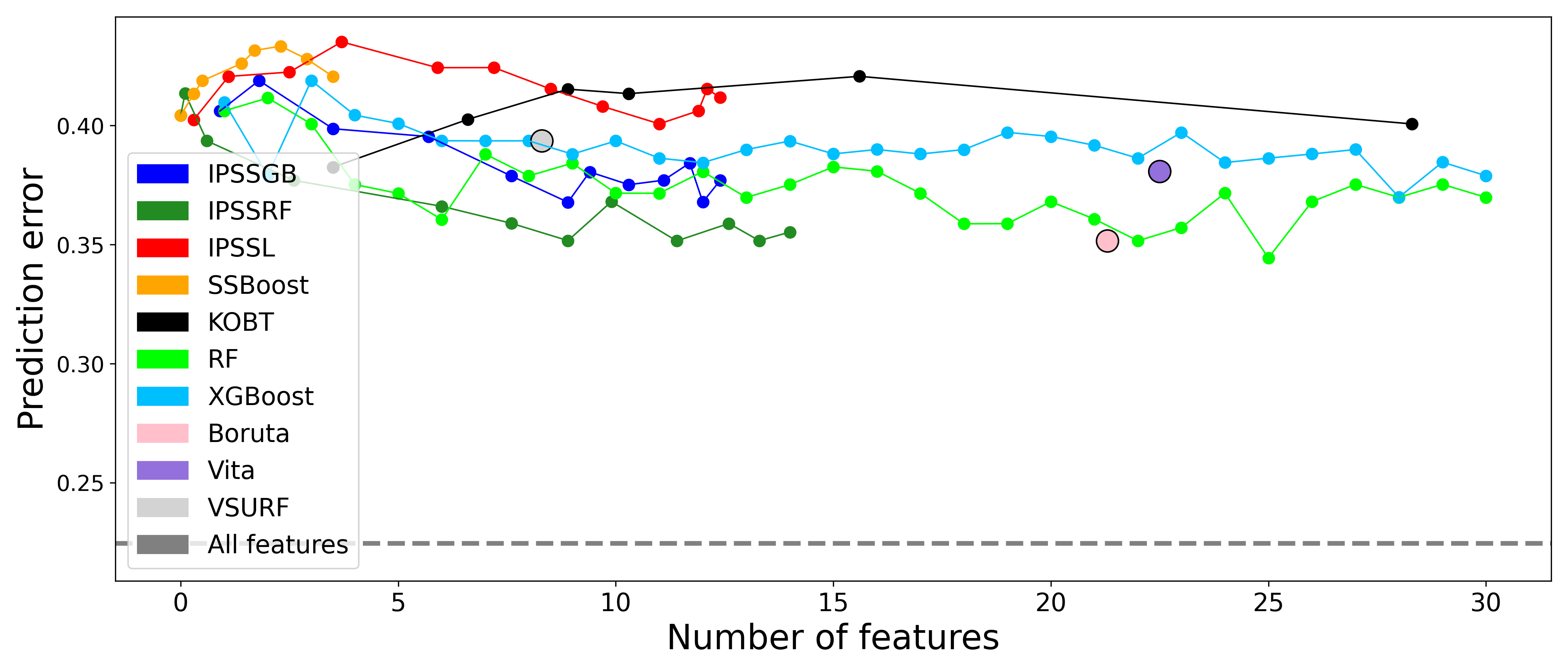
Figure S8. RNA-seq and prognosis. No method does well at predicting prognosis relative to the full dataset. This is unsurprising, given the many factors that can contribute to poor outcomes which are unlikely to be captured by RNA-seq data alone. Nevertheless, several of the genes identified by the various feature selection methods do appear to be related to ovarian cancer prognosis; see Table S5.

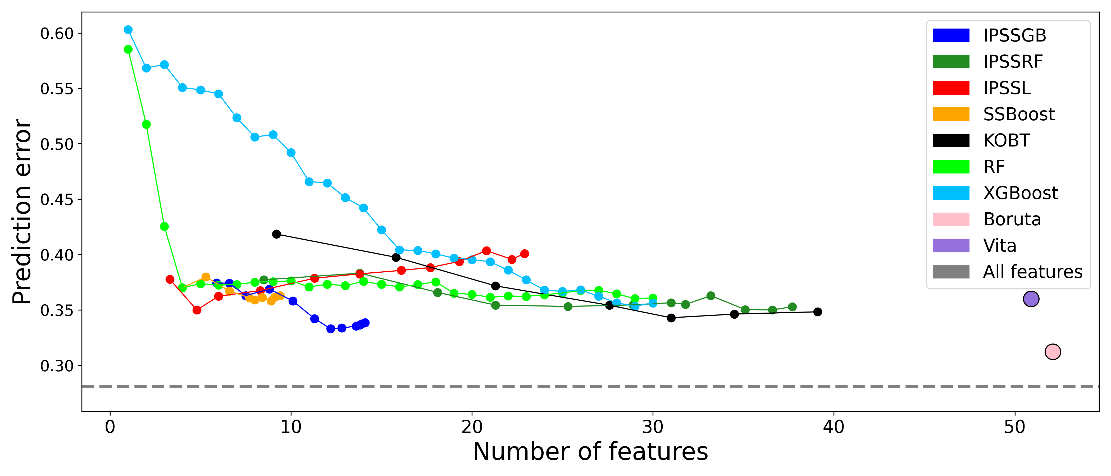
Figure S9. RNA-seq and AKT2. As in several of the other studies, IPSSGB achieves superior predictive performance with fewer features compared to other methods.

IPSSGB	IPSSRF	IPSSL
SUPT5H(0.01)	SUPT5H(0.01)	SUPT5H(0.02)
EGLN2(0.01)	PAK4(0.01)	EGLN2(0.02)
PAK4(0.01)	ADCK4(0.01)	ADCK4(0.02)
ADCK4(0.01)	EGLN2(0.01)	BLVRB(0.02)
BLVRB(0.01)	ZNF574(0.01)	SPSB3(0.03)
ITPKC(0.02)	GSK3A(0.01)	HKR1(0.03)
HKR1(0.04)	SARS2(0.01)	CAV2(0.04)
ZMYND17(0.14)	ITPKC(0.01)	MAP3K10(0.07)
U2AF2(0.19)	CLPTM1(0.01)	ACRC(0.08)
SPSB3(0.2)	ZNF526(0.01)	ITPKC(0.09)

Table S6. RNA-seq and AKT2. Top ranked genes for each method in terms of their $q$-values, shown in parentheses.

References

- Biau and Scornet (2016) G. Biau and E. Scornet. A random forest guided tour. Test, 25:197–227, 2016.
- Breiman (2001) L. Breiman. Random forests. Machine learning, 45:5–32, 2001.
- Candes et al. (2018) E. Candes, Y. Fan, L. Janson, and J. Lv. Panning for gold: ‘model-x’ knockoffs for high dimensional controlled variable selection. Journal of the Royal Statistical Society Series B: Statistical Methodology, 80(3):551–577, 2018.
- Chan et al. (2009) L. F. Chan, T. R. Webb, T.-T. Chung, E. Meimaridou, S. N. Cooray, L. Guasti, J. P. Chapple, M. Egertová, M. R. Elphick, M. E. Cheetham, et al. Mrap and mrap2 are bidirectional regulators of the melanocortin receptor family. Proceedings of the National Academy of Sciences, 106(15):6146–6151, 2009.
- Chen and Guestrin (2016) T. Chen and C. Guestrin. Xgboost: A scalable tree boosting system. In Proceedings of the 22nd acm sigkdd international conference on knowledge discovery and data mining, pages 785–794, 2016.
- Coleman et al. (2022) T. Coleman, W. Peng, and L. Mentch. Scalable and efficient hypothesis testing with random forests. Journal of Machine Learning Research, 23(170):1–35, 2022.
- Degenhardt et al. (2019) F. Degenhardt, S. Seifert, and S. Szymczak. Evaluation of variable selection methods for random forests and omics data sets. Briefings in bioinformatics, 20(2):492–503, 2019.
- Dou et al. (2020) Y. Dou, F. Chen, Y. Lu, H. Qiu, and H. Zhang. Effects of wnt/-catenin signal pathway regulated by mir-342-5p targeting cbx2 on proliferation, metastasis and invasion of ovarian cancer cells. Cancer Management and Research, pages 3783–3794, 2020.
- Friedman (2001) J. H. Friedman. Greedy function approximation: a gradient boosting machine. Annals of statistics, pages 1189–1232, 2001.
- Fu et al. (2012) X. Fu, J. Tian, L. Zhang, Y. Chen, and Q. Hao. Involvement of microrna-93, a new regulator of pten/akt signaling pathway, in regulation of chemotherapeutic drug cisplatin chemosensitivity in ovarian cancer cells. FEBS letters, 586(9):1279–1286, 2012.
- Genuer et al. (2010) R. Genuer, J.-M. Poggi, and C. Tuleau-Malot. Variable selection using random forests. Pattern recognition letters, 31(14):2225–2236, 2010.
- Ghafouri-Fard et al. (2022) S. Ghafouri-Fard, T. Khoshbakht, B. M. Hussen, S. Sarfaraz, M. Taheri, and S. A. Ayatollahi. Circ_cdr1as: A circular rna with roles in the carcinogenesis. Pathology-Research and Practice, 236:153968, 2022.
- Hastie et al. (2009) T. Hastie, R. Tibshirani, J. H. Friedman, and J. H. Friedman. The elements of statistical learning: data mining, inference, and prediction, volume 2. Springer, 2009.
- Hofner and Hothorn (2017) B. Hofner and T. Hothorn. stabs: Stability selection with error control. R package version 0.6-3, 2017.
- Hofner et al. (2014) B. Hofner, A. Mayr, N. Robinzonov, and M. Schmid. Model-based boosting in r: a hands-on tutorial using the r package mboost. Computational statistics, 29:3–35, 2014.
- Hofner et al. (2015) B. Hofner, L. Boccuto, and M. Göker. Controlling false discoveries in high-dimensional situations: boosting with stability selection. BMC Bioinformatics, 16:1–17, 2015.
- Hu et al. (2019) Y. Hu, Q. Zhang, J. Cui, Z.-J. Liao, M. Jiao, Y.-B. Zhang, Y.-H. Guo, and Y.-M. Gao. Oncogene mir-934 promotes ovarian cancer cell proliferation and inhibits cell apoptosis through targeting brms1l. European Review for Medical & Pharmacological Sciences, 23(13), 2019.
- Huynh-Thu et al. (2012) V. A. Huynh-Thu, Y. Saeys, L. Wehenkel, and P. Geurts. Statistical interpretation of machine learning-based feature importance scores for biomarker discovery. Bioinformatics, 28(13):1766–1774, 2012.
- Janitza et al. (2018) S. Janitza, E. Celik, and A.-L. Boulesteix. A computationally fast variable importance test for random forests for high-dimensional data. Advances in Data Analysis and Classification, 12(4):885–915, 2018.
- Jiang et al. (2021) T. Jiang, Y. Li, and A. A. Motsinger-Reif. Knockoff boosted tree for model-free variable selection. Bioinformatics, 37(7):976–983, 2021.
- Jin et al. (2014) M. Jin, Z. Yang, W. Ye, H. Xu, and X. Hua. Microrna-150 predicts a favorable prognosis in patients with epithelial ovarian cancer, and inhibits cell invasion and metastasis by suppressing transcriptional repressor zeb1. PloS one, 9(8):e103965, 2014.
- Kandettu et al. (2022) A. Kandettu, D. Adiga, V. Devi, P. S. Suresh, S. Chakrabarty, R. Radhakrishnan, and S. P. Kabekkodu. Deregulated mirna clusters in ovarian cancer: Imperative implications in personalized medicine. Genes & Diseases, 9(6):1443–1465, 2022.
- Kim et al. (2017) T. H. Kim, J.-Y. Jeong, J.-Y. Park, S.-W. Kim, J. H. Heo, H. Kang, G. Kim, and H. J. An. mir-150 enhances apoptotic and anti-tumor effects of paclitaxel in paclitaxel-resistant ovarian cancer cells by targeting notch3. Oncotarget, 8(42):72788, 2017.
- Kursa et al. (2010) M. B. Kursa, A. Jankowski, and W. R. Rudnicki. Boruta–a system for feature selection. Fundamenta Informaticae, 101(4):271–285, 2010.
- Lee et al. (2012) H. Lee, C. S. Park, G. Deftereos, J. Morihara, J. E. Stern, S. E. Hawes, E. Swisher, N. B. Kiviat, and Q. Feng. Microrna expression in ovarian carcinoma and its correlation with clinicopathological features. World journal of surgical oncology, 10:1–10, 2012.
- Lee et al. (2006) S.-I. Lee, H. Lee, P. Abbeel, and A. Y. Ng. Efficient -regularized logistic regression. In Proceedings of the 21st National Conference on Artificial Intelligence (AAAI), volume 6, pages 401–408, 2006.
- Liu et al. (2019) B. Liu, J. Zhang, and D. Yang. mir-96-5p promotes the proliferation and migration of ovarian cancer cells by suppressing caveolae1. Journal of Ovarian Research, 12:1–9, 2019.
- Louppe et al. (2013) G. Louppe, L. Wehenkel, A. Sutera, and P. Geurts. Understanding variable importances in forests of randomized trees. Advances in neural information processing systems, 26, 2013.
- Meinshausen and Bühlmann (2010) N. Meinshausen and P. Bühlmann. Stability selection. Journal of the Royal Statistical Society Series B: Statistical Methodology, 72(4):417–473, 2010.