Deep Koopman-layered Model with Universal Property Based on Toeplitz Matrices

Abstract

We propose deep Koopman-layered models with learnable parameters in the form of Toeplitz matrices for analyzing the dynamics of time-series data. The proposed model has both theoretical solidness and flexibility. By virtue of the universal property of Toeplitz matrices and the reproducing property underlined in the model, we can show its universality and the generalization property. In addition, the flexibility of the proposed model enables the model to fit time-series data coming from nonautonomous dynamical systems. When training the model, we apply Krylov subspace methods for efficient computations. In addition, the proposed model can be regarded as a neural ODE-based model. In this sense, the proposed model establishes a new connection among Koopman operators, neural ODEs, and numerical linear algebraic methods.

1 Introduction

Koopman operator has been one of the important tools in machine learning (Kawahara, 2016; Ishikawa et al., 2018; Lusch et al., 2017; Brunton & Kutz, 2019; Hashimoto et al., 2020). Koopman operators are linear operators that describe the composition of functions and are applied to analyzing time-series data generated by nonlinear dynamical systems (Koopman, 1931; Budišić et al., 2012; Klus et al., 2020; Giannakis & Das, 2020; Mezić, 2022). By computing the eigenvalues of Koopman operators, we can understand the long-term behavior of the undelined dynamical systems. An important feature of Applying Koopman operators is that we can estimate them with given time-series data through fundamental linear algebraic tools such as projection. A typical approach to estimate Koopman operators is extended dynamical mode decomposition (EDMD) (Williams et al., 2015). For EDMD, we need to choose the dictionary functions to determine the representation space of the Koopman operator, and what choice of them gives us a better estimation is far from trivial. In addition, since we construct the estimation in an analytical way, the model is not flexible enough to incorporate additional information about dynamical systems. With EDMD as a starting point, many DMD-based methods are proposed (Kawahara, 2016; Colbrook & Townsend, 2024; Schmid, 2022). For autonomous systems, we need to estimate a single Koopman operator. In this case, Ishikawa et al. (2024) proposed to choose derivatives of kernel functions as dictionary functions based on the theory of Jet spaces. Several works deal with nonautonomous systems. Maćešić et al. (2018) applied EDMD to estimate a time-dependent Koopman operator for each time window. However, as far as we know, no existing works show proper choices of dictionary functions for nonautonomous systems based on theoretical analysis. In addition, since each Koopman operator for a time window is estimated individually in these frameworks, we cannot take the information of other Koopman operators into account.

To find a proper representation space and gain the flexibility of the model, neural network-based Koopman methods have been proposed (Lusch et al., 2017; Azencot et al., 2020; Shi & Meng, 2022). These methods set the encoder from the data space to the representation space where the Koopman operator is defined, and the decoder from the representation space to the data space, as deep neural networks. Then, we train them. Neural network-based Koopman methods for nonautonomous systems have also been proposed. Liu et al. (2023) proposed to decompose the Koopman operator into a time-invariant part and a time-variant part. The time-variant part of the Koopman operator is constructed individually for each time window using EDMD. Xiong et al. (2024) assumed the ergodicity of the dynamical system and considered time-averaged Koopman operators for nonautonomous dynamical systems. However, their theoretical properties have not been fully understood, and since the representation space changes as the learning process proceeds, their theoretical analysis is challenging.

In this work, we propose a framework that estimates multiple Koopman operators over time with the Fourier basis representation space and learnable Toeplitz matrices. Using our framework, we can estimate multiple Koopman operators simultaneously and can capture the transition of properties of data along time via multiple Koopman operators. We call each Koopman operator the Koopman-layer, and the whole model the deep Koopman-layered model. The proposed model has both theoretical solidness and flexibility. We show that the Fourier basis is a proper basis for constructing the representation space even for nonautonomous dynamical systems in the sense that we can show its theoretical properties such as universality and generalization bound. In addition, the proposed model has learnable parameters, which makes the model more flexible to fit nonautonomous dynamical systems than the analytical methods such as EDMD. The proposed model resolves the issue of theoretical analysis for the neutral network-based methods and that of the flexibility for the analytical methods simultaneously.

We show that each Koopman operator is represented by the exponential of a matrix constructed with Toeplitz matrices and diagonal matrices. This allows us to apply Krylov subspace methods (Gallopoulos & Saad, 1992; Güttel, 2013; Hashimoto & Nodera, 2016) to compute the estimation of Koopman operators with low computational costs. By virtue of the universal property of Toeplitz matrices (Ye & Lim, 2016), we can show the universality of the proposed model with a linear algebraic approach. We also show a generalization bound of the proposed model using a reproducing kernel Hilbert space (RKHS) associated with the Fourier functions. We can analyze both the universality and generalization error with the same framework.

The proposed model can also be regarded as a neural ODE-based model (Chen et al., 2018; Teshima et al., 2020a; Li et al., 2023). While in the existing method, we train the models with numerical analysis approaches, in the proposed method, we train the models with a numerical linear algebraic approach. The universality and generalization results of the proposed model can also be seen as those for the neural ODE-based models. Our method sheds light on a new linear algebraic approach to the design of neural ODEs.

Our contributions are summarized as follows:

• We propose a model for analyzing nonautonomous dynamical systems that has both theoretical solidness and flexibility. We show that the Fourier basis provides us with a proper representation space, in the sense that we can show the universality and the generalization bound regarding the model. As for the flexibility, we can learn multiple Koopman operators simultaneously, which enables us to extract the transition of properties of dynamical systems along time.

• We apply Krylov subspace methods to compute the estimation of Koopman operators. This establishes a new connection between Koopman operator theoretic approaches and Krylov subspace methods, which opens up future directions for extracting further information about dynamical systems using numerical linear algebraic approaches.

• We provide a new implementation method for neural ODEs purely with numerical linear algebraic approaches, not with numerical analysis approaches.

2 Preliminary

In this section, we provide notations and fundamental notions required in this paper.

2.1 Notations

In this paper, we use a generalized concept of matrices. For a finite index set $N\subset\mathbb{Z}^{d}$ and $a_{j,l}\in\mathbb{C}$ $(j,l\in N)$, we call $A=[a_{j,l}]_{j,l\in N}$ an $N$ by $N$ matrix and denote by $\mathbb{C}^{N\times N}$ the space of all $N$ by $N$ matrices. Indeed, by constructing a bijection $I:N\to\{1,\ldots,|N|\}$ and setting $\tilde{a}_{I(j),I(l)}=a_{j,l}$, we obtain a standard matrix $[\tilde{a}_{I(j),I(l)}]_{I(j),I(l)}$ corresponding to $A$.

2.2 $L^{2}$ space and Reproducing kernel Hilbert space on the torus

We consider two function spaces, the $L^{2}$ space and RKHS, in this paper. Let $\mathbb{T}$ be the torus $\mathbb{R}/2\pi\mathbb{Z}$. We denote by $L^{2}(\mathbb{T}^{d})$ the space of square-integrable complex-valued functions on $\mathbb{T}^{d}$, equipped with the Lebesgue measure. As for the RKHS, let $\kappa:\mathbb{T}^{d}\times\mathbb{T}^{d}\to\mathbb{C}$ be a positive definite kernel, which satisfies the following two properties:

1. ${\kappa}(x,y)=\overline{\kappa(y,x)}$  for $x,y\in\mathbb{T}^{d}$,

2. $\sum_{n,m=1}^{N}\!\overline{c_{n}}c_{m}\kappa(x_{n},x_{m})\!\geq\!0$  for $N\in\mathbb{N}$, $c_{n}\in\mathbb{C}$, $x_{n}\in\mathbb{T}$.

Let ${\phi}$ be a map defined as $\phi(x)=\kappa(\cdot,x)$, which is called the feature map. The RKHS $\mathcal{H}_{\kappa}$ is the Hilbert space spanned by $\{\phi(x)\,\mid\,x\in\mathbb{T}^{d}\}$. The inner product $\left\langle\cdot,\cdot\right\rangle:\mathcal{H}_{\kappa}\times\mathcal{H}_{\kappa}\to\mathbb{C}$ in $\mathcal{H}_{\kappa}$ is defined as

$$\bigg{\langle}\sum_{n=1}^{N}c_{n}{\phi}(x_{n}),\sum_{m=1}^{M}d_{m}{\phi}(y_{m})\bigg{\rangle}=\sum_{n=1}^{N}\sum_{m=1}^{M}\overline{c_{n}}d_{m}\kappa(x_{n},y_{m})$$

for $c_{n},d_{n}\in\mathbb{C}$ and $x_{n},y_{n}\in\mathbb{T}^{d}$. Note that by the definition of $\kappa$, $\left\langle\cdot,\cdot\right\rangle$ is well-defined and satisfies the axiom of inner products. An important property for RKHSs is the reproducing property. For $x\in\mathbb{T}^{d}$ and $v\in\mathcal{H}_{\kappa}$, we have $\left\langle\phi(x),v\right\rangle=v(x)$, which is useful for deriving a generalization bound.

2.3 Koopman generator and operator

Consider an ODE $\frac{\mathrm{d}x}{\mathrm{d}t}(t)=f(x(t))$ on $\mathbb{T}^{d}$. Let $g:\mathbb{R}\times\mathbb{T}^{d}$ be the flow of the ODE, that is, $g$ satisfies $g(0,x)=x$ and $g(s,g(t,x))=g(s+t,x)$ for $x\in\mathbb{T}^{d}$. We assume $g$ is continuous and invertible. For $t\in\mathbb{R}$, we define the Koopman operator $K^{t}$ on $L^{2}(\mathbb{T}^{d})$ by the composition with $g(t,\cdot)$ as $K^{t}h(x)=h(g(t,x))$ for $h\in L^{2}(\mathbb{T}^{d})$ and $x\in\mathbb{T}^{d}$. The Koopman operator is a linear operator that maps a function $h$ to a function $h(g(t,\cdot))$. Note that the Koopman operator $K^{t}$ is linear even if $g(t,\cdot)$ is nonlinear. Since $K^{t}$ depends on $t$, we can consider the family of Koopman operators $\{K^{t}\}_{t\in\mathbb{R}}$. For $h\in C^{1}(\mathbb{T}^{d})$, where $C^{1}(\mathbb{T}^{d})$ is the space of continuous differentiable functions on $\mathbb{T}^{d}$, let $L$ be the linear operator defined as

$$Lh=\lim_{t\to\infty}\frac{K^{t}h-h}{t},$$

where the limit is by means of $L^{2}(\mathbb{T})$. We call $L$ the Koopman generator. We write $K^{t}=\mathrm{e}^{tL}$. If $L$ is bounded, then it coincides with the standard definition $\mathrm{e}^{tL}=\sum_{i=1}^{\infty}(tL)^{i}/i!$. If $L$ is unbounded, it can be justified by approximating $L$ by a sequence of bounded operators and considering the strong limit of the sequence of the exponential of the bounded operators (Yosida, 1980).

3 Deep Koopman-layered model

We propose deep Koopman-layered models based on the Koopman operator theory, which have both theoretical solidness and flexibility.

3.1 Multiple dynamical systems and Koopman generators

Consider $J$ ODEs $\frac{\mathrm{d}x}{\mathrm{d}t}(t)=f_{j}(x(t))$ on $\mathbb{T}^{d}$ for $j=1,\ldots,J$. Let $g_{j}:\mathbb{R}\times\mathbb{T}^{d}$ be the flow of the $j$th ODE. For $v\in L^{2}(\mathbb{T}^{d})$, consider the following model:

$$G(x)=v\circ g_{J}(t_{J},\cdot)\circ\cdots\circ g_{1}(t_{1},\cdot)(x)=v(g_{J}(t_{J},\cdots g_{1}(t_{1},x))).$$ (1)

This model describes a switching dynamical system, and also is regarded as a discrete approximation of a nonautonomous dynamical system.

Remark 1

Since we are focusing on the complex-valued function space $L^{2}(\mathbb{T})$, $G$ itself is a complex-valued function. However, we can easily extend the model to the flow $g_{J}(t_{J},\cdot)\circ\cdots\circ g_{1}(t_{1},\cdot)$, which is a map from $\mathbb{T}^{d}$ to $\mathbb{T}^{d}$. We can obtain a complex-valued function on $\mathbb{T}^{d+1}$ that describes a map from $\mathbb{T}^{d}$ to $\mathbb{T}^{d}$. Indeed, let $\tilde{g}_{j}(x,y)=[g_{j}(t_{j},x),y]$ for $x\in\mathbb{T}^{d}$ and $y\in\mathbb{T}$. Let $\tilde{v}$ be a function that satisfies $\tilde{v}(x,k/d)=x_{k}$, and let $G=\tilde{v}\circ\tilde{g}_{J}\circ\cdots\circ\tilde{g}_{1}$. Then, $G(\cdot,k/d)$ is the $k$th element of $g_{J}(t_{J},\cdot)\circ\cdots\circ g_{1}(t_{1},\cdot)$.

3.2 Approximation of Koopman generators using Toeplitz matrices

We consider training the model (1) using given time-series data. For this purpose, we apply the Koopman operator theory. Let $L_{j}$ be the Koopman generator associated with the flow $g_{j}$. Since the Koopman operator $K^{t_{j}}_{j}$ of $g_{j}$ is represented as $\mathrm{e}^{t_{j}L_{j}}$, the model (1) is represented as

$$G=\mathrm{e}^{t_{1}L_{1}}\cdots\mathrm{e}^{t_{J}L_{J}}v.$$

To deal with the Koopman generators defined on the infinite-dimensional space, we approximate them using Fourier functions. Let $q_{n}(x)=\mathrm{e}^{\mathrm{i}n\cdot x}$ for $n\in\mathbb{Z}^{d}$ and $x\in\mathbb{T}^{d}$, where $\mathrm{i}$ is the imaginary unit. Let $M^{j}_{r}\subset\mathbb{Z}^{d}$ be a finite index set for $r=1,\ldots,R_{j}$. We set the $k$th element of the function $f_{j}$ in the ODE as

$$\sum_{m_{R_{j}}\in M^{j}_{R_{j}}}a^{j,k}_{m_{R_{j}},R_{j}}q_{m_{R_{j}}}\cdots\sum_{m_{1}\in M^{j}_{1}}a^{j,k}_{m_{1},1}q_{m_{1}}$$ (2)

with $a^{j,k}_{m_{r},r}\in\mathbb{C}$, the product of weighted sums of Fourier functions. Then, we approximate the Koopman generator $L_{j}$ by projecting the input vector onto the space $V_{N}:=\operatorname{Span}\{q_{n}\,\mid\,n\in N\}$, where $N\subset\mathbb{Z}^{d}$ is a finite index set, applying $L_{j}$, and projecting it back to $V_{N}$ as $Q_{N}Q_{N}^{*}L_{j}Q_{N}Q_{N}^{*}$. Here, $Q_{N}:\mathbb{C}^{N}\to V_{N}$ is the linear operator defined as $Q_{N}c=\sum_{n\in N}c_{n}q_{n}$ for $c=(c_{n})_{n\in N}\in\mathbb{C}^{N}$ and ^∗ is the adjoint. Note that $Q_{N}Q_{N}^{*}$ is the projection onto $V_{N}$. Then, the representation matrix $Q_{N}^{*}L_{j}Q_{N}$ of the approximated Koopman generator $Q_{N}Q_{N}^{*}L_{j}Q_{N}Q_{N}^{*}$ is written as follows. Throughout the paper, all the proofs are documented in Appendix A.

Proposition 2

The $(n,l)$-entry of the representation matrix $Q_{N}^{*}L_{j}Q_{N}$ of the approximated operator is

$$\sum_{k=1}^{d}\sum_{n_{R_{j}}-l\in M^{j}_{R_{j}}}\sum_{n_{R_{j}-1}-n_{R_{j}}\in M^{j}_{R_{j}-1}}\cdots\sum_{n_{2}-n_{3}\in M^{j}_{2}}\sum_{n-n_{2}\in M^{j}_{1}}$$

$$\qquad\qquad\qquad\qquad a^{j,k}_{n_{R_{j}}-l,R_{j}}a^{j,k}_{n_{R_{j}-1}-n_{R_{j}},R_{j-1}}\cdots a^{j,k}_{n_{2}-n_{3},2}a^{j,k}_{n-n_{2},1}\mathrm{i}l_{k},$$ (3)

where $l_{k}$ is the $k$th element of the index $l\in\mathbb{Z}^{d}$. Moreover, we set $n_{r}=m_{R_{j}}+\cdots+m_{r}+l$, thus $n_{1}=n$, $m_{r}=n_{r}-n_{r+1}$ for $r=1,\ldots,R_{j}-1$, and $m_{R_{j}}=n_{R_{j}}-l$.

Note that since the sum involves the differences of indices, it can be written using Toeplitz matrices, whose $(n,l)$-entry depends only on $n-l$. We approximate the sum appearing in Eq. (3) by restricting the index $n_{r}$ to $N$, combine with the information of time $t_{j}$, and set a matrix $\mathbf{L}_{j}\in\mathbb{C}^{N\times N}$ as

$$\mathbf{L}_{j}=t_{j}\sum_{k=1}^{d}A_{1}^{j,k}\cdots A_{R_{j}}^{j,k}D_{k},$$

where $A_{r}^{j,k}$ is the Toeplitz matrix defined as $A_{r}^{j,k}=[a_{n-l,r}^{j,k}]_{n,l\in N}$ and $D_{k}$ is the diagonal matrix defined as $(D_{k})_{l,l}=\mathrm{i}l_{k}$. We finally regard $Q_{N}\mathbf{L}_{j}Q_{N}^{*}$ as an approxitation of the Koopman genertor $L_{j}$.

Then, we construct the approximation $\mathbf{G}$ of $G$, defined in Eq. (1), as

$$\mathbf{G}=\mathrm{e}^{Q_{N}\mathbf{L}_{1}Q_{N}^{*}}\cdots\mathrm{e}^{Q_{N}\mathbf{L}_{J}Q_{N}^{*}}v=Q_{N}\mathrm{e}^{\mathbf{L}_{1}}\cdots\mathrm{e}^{\mathbf{L}_{J}}Q_{N}^{*}v.$$ (4)

We call the model $\mathbf{G}$ deep Koopman-layered model.

To compute the product of the matrix exponential $\mathrm{e}^{\mathbf{L}_{j}}$ and the vector $\mathrm{e}^{\mathbf{L}_{j+1}}\cdots\mathrm{e}^{\mathbf{L}_{J}}Q_{N}^{*}v$, we can use Krylov subspace methods. If the number of indices for describing $f_{j}$ is smaller than that for describing the whole model, i.e., $|M^{j}_{r}|\ll|N|$, then the Toeplitz matrix $A^{j,k}_{r}$ is sparse. In this case, the matrix-vector product can be computed with the computational cost of $O(\sum_{r=1}^{R_{j}}|M^{j}_{r}||N|)$. Thus, one iteration of the Krylov subspace method costs $O(\sum_{r=1}^{R_{j}}|M^{j}_{r}||N|)$, which makes the computation efficient compared to direct methods without taking the structure of the matrix into account, whose computational cost results in $O(|N|^{3})$.

Remark 3

To restrict $f_{j}$ to be a real-valued map and reduce the number of parameters $a_{m,r}^{j,k}$, we can set $M^{j}_{r}$ as $\{-m^{j}_{1,r},\ldots,m^{j}_{1,r}\}\times\cdots\times\{-m^{j}_{d,r},\ldots,m^{j}_{d,r}\}$ for $m^{j}_{k,r}\in\mathbb{N}$ for $k=1,\ldots,d$. In addition, we set $a_{m,r}^{j,k}=\overline{a_{-m,r}^{j,k}}$ for $m\in M_{r}^{j}$. Then, we have $a_{m,r}^{j,k}q_{m}=\overline{a_{-m,r}^{j,k}q_{-m}}$, and $f_{j}$ is real-valued.

Remark 4

An advantage of applying Koopman operators is that their spectra describe the properties of dynamical systems. For example, if the dynamical system is measure preserving, then the corresponding Koopman operator is unitary. Since each Koopman layer is an estimation of the Koopman operator, we can analyze time-series data coming from nonsutonomous dynamical systems by computing the eigenvalues of the Koopman layers. We will observe the eigenvalues of Koopman layers numerically in Subsection 6.2.

4 Universality

In this section, we show the universal property of the proposed deep Koopman-layered model. We can interpret the model $\mathbf{G}$ as the approximation of the target function by transforming the function $v$ into the target function using the linear operator $Q_{N}\mathrm{e}^{\mathbf{L}_{1}}\cdots\mathrm{e}^{\mathbf{L}_{J}}Q_{N}^{*}$. If we can represent any linear operator by $\mathrm{e}^{\mathbf{L}_{1}}\cdots\mathrm{e}^{\mathbf{L}_{J}}$, then we can transform $v$ into any target function in $V_{N}$, which means we can approximate any function as $N$ goes to the whole set $\mathbb{Z}^{d}$. Thus, this property corresponds to the universality of the model. In Section 3, by constructing the model with the matrix $\mathrm{e}^{\mathbf{L}_{1}}\cdots\mathrm{e}^{\mathbf{L}_{J}}$ based on the Koopman operators with the Fourier functions, we restrict the number of parameters of the linear operator that transforms $v$ into the target function. The universality of the model means that this restriction is reasonable in the sense of representing the target functions using the deep Koopman-layered model.

Let $T(N,\mathbb{C})=\{\sum_{k=1}^{d}A_{1}^{k}\cdots A_{R_{k}}^{k}D_{k},\,\mid\,R_{k}\in\mathbb{N},\ A_{1}^{k}\cdots A_{R_{k}}^{k}\in\mathbb{C}^{N\times N}\mbox{ : Toeplitz}\}$. Let $L_{0}^{2}(\mathbb{T}^{d})=\overline{\operatorname{Span}\{q_{n}\,\mid\,n\neq 0\}}$ be the space of $L^{2}$ functions whose average is $0$. We show the following fundamental result of the universality of the model:

Theorem 5

Assume $v\in L_{0}^{2}(\mathbb{T}^{d})$ and $v\neq 0$. For any $f\in L_{0}^{2}(\mathbb{T}^{d})$ with $f\neq 0$ and for any $\epsilon>0$, there exist a finite set $N\subset\mathbb{Z}\setminus\{0\}$, a positive integer $J$, and matrices $\mathbf{L}_{1},\ldots,\mathbf{L}_{J}\in T(N,\mathbb{C})$ such that $\|f-\mathbf{G}\|\leq\epsilon$ and $\mathbf{G}=Q_{N}\mathrm{e}^{\mathbf{L}_{1}}\cdots\mathrm{e}^{\mathbf{L}_{J}}Q_{N}^{*}v$.

Theorem 5 is for a single function $f$, but applying Theorem 5 for each component of $\mathbf{G}$, we obtain the following result for the flow $g_{\tilde{J}}(t_{\tilde{J}},\cdot)\circ\cdots\circ g_{1}(t_{1},\cdot)$ with $\tilde{J}\in\mathbb{N}$, which is considered in Eq. (1).

Corollary 6

Assume $v\in L_{0}^{2}(\mathbb{T}^{d})$ and $v\neq 0$. For any sequence $g_{1}(t_{1},\cdot),\ldots,g_{\tilde{J}}(t_{\tilde{J}},\cdot)$ of flows that satisfies $v\circ g_{\tilde{J}}(t_{\tilde{J}},\cdot)\circ\cdots\circ g_{j}(t_{j},\cdot)\in L^{2}_{0}(\mathbb{T}^{d})$ and $v\circ g_{\tilde{J}}(t_{\tilde{J}},\cdot)\circ\cdots\circ g_{j}(t_{j},\cdot)\neq 0$ for $j=1,\ldots\tilde{J}$, and for any $\epsilon>0$, there exist a finite set $N\subset\mathbb{Z}\setminus\{0\}$, integers $0<J_{1}<\cdots<J_{\tilde{J}}$, and matrices $\mathbf{L}_{1},\ldots,\mathbf{L}_{J_{\tilde{J}}}\in T(N,\mathbb{C})$ such that $\|v\circ g_{\tilde{J}}(t_{\tilde{J}},\cdot)\circ\cdots\circ g_{j}(t_{j},\cdot)-\mathbf{G}_{j}\|\leq\epsilon$ and $\mathbf{G}_{j}=Q_{N}\mathrm{e}^{\mathbf{L}_{J_{j-1}+1}}\cdots\mathrm{e}^{\mathbf{L}_{J_{\tilde{J}}}}Q_{N}^{*}v$ for $j=1,\ldots,\tilde{J}$, where $J_{0}=1$.

Remark 7

The function space $L_{0}^{2}(\mathbb{T}^{d})$ for the target function is not restrictive. By adding a constant to the functions in $L_{0}^{2}(\mathbb{T}^{d})$, we can represent any function in $L^{2}(\mathbb{T}^{d})$. Thus, by adding one additional learnable parameter $c\in\mathbb{C}$ to the model $\mathbf{G}$ in Theorem 5 and consider the model $\mathbf{G}(x)+c$ for an input $x\in\mathbb{T}^{d}$, we can represent any function in $L^{2}(\mathbb{T}^{d})$.

The proof of Theorem 5 is obtained by a linear algebraic approach. By virtue of setting $f_{j}$ as the product of weighted sums of Fourier functions as explained in Eq. (2), the approximation of the Koopman generator is composed of Toeplitz matrices. As a result, we can apply the following proposition regarding Toeplitz matrices by Ye & Lim (2016, Theorem 2).

Proposition 8

For any $B\in\mathbb{C}^{N\times N}$, there exists $R=\lfloor|N|\rfloor+1$ Toeplitz matrices $A_{1},\ldots,A_{R}$ such that $B=A_{1}\cdots A_{R}$.

We use Proposition 8 to show the following lemma regarding the representation with $T(N,\mathbb{C})$.

Lemma 9

Assume $N\subset\mathbb{Z}^{d}\setminus\{0\}$. Then, we have $\mathbb{C}^{N\times N}=T(N,\mathbb{C})$.

Since $\mathbb{C}^{N\times N}$ is a Lie algebra and the corresponding Lie group $GL(N,\mathbb{C})$, the group of nonsingular $N$ by $N$ matrices, is connected, we have the following lemma (Hall, 2015, Corollary 3.47).

Lemma 10

We have $GL(N,\mathbb{C})=\{\mathrm{e}^{\mathbf{L}_{1}}\cdots\mathrm{e}^{\mathbf{L}_{J}}\,\mid\,J\in\mathbb{N},\ \mathbf{L}_{1},\ldots,\mathbf{L}_{J}\in\mathbb{C}^{N\times N}\}$.

We also use the following transitive property of $GL(N,\mathbb{C})$ and finally obtain Theorem 5.

Lemma 11

For any $\mathbf{u},\mathbf{v}\in\mathbb{C}^{N}\setminus\{0\}$, there exists $A\in GL(N,\mathbb{C})$ such that $\mathbf{u}=A\mathbf{v}$.

Training deep Koopman-layered model with time-series data

Based on Corollary 6, we can train the deep Koopman-layered model using time-series data as follows: We first fix the final nonlinear transform $v$ in the model $\mathbf{G}$ taking Remark 1 into account, the number of layers $\tilde{J}$, and the index sets $N$, $M_{r}^{j}$. We input a family of time-series data $\{x_{s,0},\ldots,x_{s,\tilde{J}}\}_{s=1}^{S}$ to $\mathbf{G}$. We learn the parameter $a_{m,r}^{j,k}$ in $\mathbf{G}$ by minimizing $\sum_{s=1}^{S}\ell(v(x_{s,\tilde{J}}),\mathbf{G}_{j}(x_{s,j-1}))$ for $j=1,\ldots,\tilde{J}$ using an optimization method. For example, we can set an objective function $\sum_{j=1}^{\tilde{J}}\sum_{s=1}^{S}\ell(v(x_{s,\tilde{J}}),\mathbf{G}_{j}(x_{s,j-1}))$. Here $\ell:\mathbb{C}\times\mathbb{C}\to\mathbb{R}$ is a loss function. For example, we can set $\ell$ as the squared error. We will show examples of the training of deep Koopman-layered models and numerical results in Section 6.

5 Generalization bound

We investigate the generalization property of the proposed deep Koopman-layered model in this section. Our framework with Koopman operators enables us to derive a generalization bound involving the norms of Koopman operators.

Let $\mathcal{G}_{N}=\{Q_{N}\mathrm{e}^{\mathbf{L}_{1}}\cdots\mathrm{e}^{\mathbf{L}_{J}}Q_{N}^{*}v\,\mid\,\mathbf{L}_{1},\ldots,\mathbf{L}_{J}\in T(N,\mathbb{C})\}$ be the function class of deep Koopman-layered model (4). Let $\ell(\mathcal{G}_{N})=\{(x,y)\mapsto\ell(f(x),y)\,\mid\,f\in\mathcal{G}_{N}\}$ for a function $\ell$ that is bounded by $C>0$. Then, we have the following result of a generalization bound for the deep Koopman-layered model.

Proposition 12

Let $h\in\ell(\mathcal{G}_{N})$, $x$ and $y$ be random variables, $S\in\mathbb{N}$, and $x_{1},\ldots,x_{S}$ and $y_{1},\ldots,y_{S}$ be i.i.d. samples drawn from the distributions of $x$ and $y$, respectively. For any $\delta>0$, with probability at least $1-\delta$, we have

$$\mathrm{E}[h(x,y)]\leq\frac{1}{S}\sum_{s=1}^{S}h(x_{n},y_{n})+\frac{\alpha}{\sqrt{S}}\max_{j\in N}\mathrm{e}^{\tau\|j\|_{1}}\!\!\!\!\!\!\!\!\!\sup_{\mathbf{L}_{1},\ldots,\mathbf{L}_{J}\in T(N,\mathbb{C})}\!\!\!\!\!\|\mathrm{e}^{\mathbf{L}_{1}}\|\cdots\|\mathrm{e}^{\mathbf{L}_{J}}\|\,\|v\|+3C\sqrt{\frac{\log(\delta/2)}{S}}.$$

We use the Rademacher complexity to derive Proposition 12. For this purpose, we regard the model (1) as a function in an RKHS. For $j\in\mathbb{Z}^{d}$ and $x\in\mathbb{T}^{d}$, let $\tilde{q}_{j}(x)=\mathrm{e}^{-\tau\|j\|_{1}}\mathrm{e}^{\mathrm{i}j\cdot x}$, where $\tau>0$ is a fixed parameter and $\|[j_{1},\ldots,j_{d}]\|_{1}=|j_{1}|+\cdots+|j_{d}|$ for $[j_{1},\ldots,j_{d}]\in\mathbb{Z}^{d}$. Let $\kappa(x,y)=\sum_{j\in\mathbb{Z}^{d}}\overline{\tilde{q}_{j}(x)}\tilde{q}_{j}(y)$, and consider the RKHS $\mathcal{H}_{\kappa}$ associated with the kernel $\kappa$. Note that $\{\tilde{q}_{j}\,\mid\,j\in\mathbb{Z}^{d}\}$ is an orthonormal basis of $\mathcal{H}_{\kappa}$. Giannakis et al. (2022) and Das et al. (2021) used this kind of RKHSs for simulating dynamical systems on a quantum computer based on the Koopman operator theory and for approximating Koopman operators by a sequence of compact operators. Here, we use the RKHS $\mathcal{H}_{\kappa}$ for deriving a generalization bound. To regard the function $\mathbf{G}\in V_{N}=\operatorname{Span}\{q_{j}\,\mid\,j\in N\}\subset L^{2}(\mathbb{T}^{d})$ as a function in $\mathcal{H}_{\kappa}$, we define an inclusion map $\iota_{N}:V_{N}\to\mathcal{H}_{\kappa}$ as $\iota_{N}q_{j}=\mathrm{e}^{\tau\|j\|_{1}}\tilde{q}_{j}$ for $j\in N$. Then, the operator norm of $\iota_{N}$ is $\|\tau_{N}\|=\max_{j\in N}\mathrm{e}^{\tau\|j\|_{1}}$.

Let $S\in\mathbb{N}$, $\sigma_{1},\ldots,\sigma_{S}$ be i.i.d. Rademacher variables, and $x_{1},\ldots,x_{S}$ be given samples. Then, the empirical Rademacher complexity $\hat{R}_{S}(\mathcal{G}_{N})$ is bounded as follows.

Lemma 13

We have

$$\hat{R}_{S}(\mathcal{G}_{N})\leq\frac{\alpha}{\sqrt{S}}\max_{j\in N}\mathrm{e}^{\tau\|j\|_{1}}\sup_{\mathbf{L}_{1},\ldots,\mathbf{L}_{J}\in T(N,\mathbb{C})}\|\mathrm{e}^{\mathbf{L}_{1}}\|\cdots\|\mathrm{e}^{\mathbf{L}_{J}}\|\,\|v\|,$$

where $\alpha=\sum_{j\in\mathbb{Z}^{d}}\mathrm{e}^{-2\tau\|j\|_{1}}$.

We can see that the complexity of the model depends exponentially on both $N$ and $J$. Combining Lemma 4.2 in Mohri et al. (2012) and Lemma 13, we can derive Proposition 12.

Remark 14

The exponential dependence of the generalization bound on the number of layers is also typical for standard neural networks (Neyshabur et al., 2015; Bartlett et al., 2017; Golowich et al., 2018; Hashimoto et al., 2024).

Remark 15

Based on Proposition 12, we can control the generalization error by adding a regularization term to the loss function to make $\|\mathrm{e}^{\mathbf{L}_{1}}\|\cdots\|\mathrm{e}^{\mathbf{L}_{J}}\|$ smaller.

6 Numerical results

We empirically confirm the fundamental properties of the proposed deep Koopman-layered model.

6.1 Representation power and generalization

To confirm the fundamental property of the Koopman layer, we first consider an autonomous system. Consider the van der Pol oscillator on $\mathbb{T}$

$$\frac{\mathrm{d}^{2}x(t)}{\mathrm{d}t^{2}}=-\mu(1-x(t)^{2})\frac{\mathrm{d}x(t)}{\mathrm{d}t}+x(t),$$ (5)

where $\mu=3$. By setting $\mathrm{d}x/\mathrm{d}t$ as a new variable, we regard Eq. (5) as a first-ordered system on the two-dimensional space. We discretized Eq. (5) with the time-interval $\Delta t=0.01$, and generated 1000 time-series $\{x_{s,0},\ldots x_{s,100}\}$ for $s=1,\ldots,1000$ with different initial values distributed uniformly on $[-1,1]\times[-1,1]$. We added a random noise, which was drawn from the normal distribution of mean 0 and standard deviation 0.01, to each $x_{s,j}$ and set it as $\tilde{x}_{s,j}$. For training, we used the pairs $\{\tilde{x}_{s,0},\tilde{x}_{s,100}\}$ for $s=1,\ldots,1000$. Then, we trained deep Koopman-layered models on $\mathbb{T}^{3}$ by minimizing the loss $\sum_{s=1}^{1000}\|Q_{N}\mathrm{e}^{\mathbf{L}_{1}}\cdots\mathrm{e}^{\mathbf{L}_{J}}Q_{N}^{*}v(\tilde{x}_{s,0})-\tilde{x}_{s,100}\|^{2}$ using the Adam optimizer (Kingma & Ba, 2015) with the learning rate $0.001$. We created data for testing in the same manner as the training dataset. We set $v(x,y)=\sin(y)x_{1}+\cos(y)x_{2}$ for $x=[x_{1},x_{2}]\in\mathbb{T}^{2}$ and $y\in\mathbb{T}$. Note that based on Remark 1, we constructed Kooman-layers on $\mathbb{T}^{d+1}$ for the input dimension $d$, and we designed the function $v$ so that it recovers $x_{1}$ by $v(x,\pi/2)$ and $x_{2}$ by $v(x,0)$. We used the sine and cosine functions for designing $v$ since the representation space is constructed with the Fourier functions. We set $N=\{n=[n_{1},n_{2},n_{3}]\in\mathbb{Z}^{3}\,\mid\,-5\leq n_{1},n_{2},n_{3}\leq 5\}\setminus\{0\}$, $R=1$, and $M_{1}=\{n=[n_{1},n_{2},n_{3}]\in\mathbb{Z}^{3}\,\mid\,-2\leq n_{1},n_{2}\leq 2,-1\leq n_{3}\leq 1\}\setminus\{0\}$ for all the layers. We applied the Arnoldi method (Gallopoulos & Saad, 1992) to compute the exponential of $\mathbf{L}_{j}$.

Figure 1 (a) shows the test error for $J=1$ and $J=2$. We can see that the performance becomes higher when $J=2$ than $J=1$. Note that Theorem 5 is a fundamental result for autonomous systems, and according to Theorem 5, we may need more than one layer even for the autonomous systems. The result reflects this theoretical result. In addition, based on Remark 15, we added the regularization term $10^{-5}(\|\mathrm{e}^{\mathbf{L}_{1}}\|+\cdots+\|\mathrm{e}^{\mathbf{L}_{J}}\|)$ and observed the behavior. We consider the case where the training data is noisy, and its sample size is small. We generated training data as above, but the sample size was 30, and the standard deviation of the noise was 0.03. We used the test data without the noise. The sample size of the test data was 1000. We set $J=3$ to consider the case where the number of parameters is large. The result is illustrated in Figure 1 (b). We can see that with the regularization, we can achieve smaller test errors than without the regularization, which implies that with the regularization, the model generalizes well.

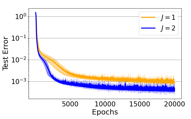
(a) Without the regularization

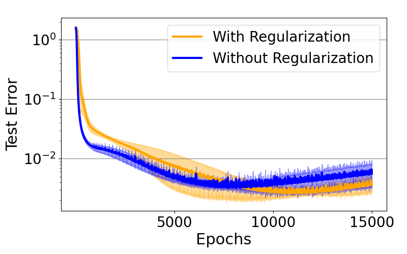
(b) With and without the regularization

Figure 1: Test error for different values of $J$ with and without the regularization based on the norms of the Koopman operators. The result is the average $\pm$ the standard deviation of three independent runs.

6.2 Eigenvalues of the Koopman-layers for nonautonomous systems

To confirm that we can extract information about the underlined nonautonomous dynamical systems of time-series data using the deep Koopman-layered model, we observed the eigenvalues of the Koopman-layers.

6.2.1 Measure-preserving dynamical system

Consider the nonautonomous dynamical system on $\mathbb{T}^{2}$

$$\bigg{(}\frac{\mathrm{d}x_{1}(t)}{\mathrm{d}t},\frac{\mathrm{d}x_{2}(t)}{\mathrm{d}t}\bigg{)}=\bigg{(}-\frac{\partial\zeta}{\partial x_{2}}(t,x(t)),\frac{\partial\zeta}{\partial x_{1}}(t,x(t))\bigg{)}=:f(t,x),$$ (6)

where $\zeta(t,[x_{1},x_{2}])=\mathrm{e}^{\kappa(\cos(x_{1}-t)+\cos x_{2})}$. Since the dynamical system $f(t,\cdot)$ is measure-preserving for any $t\in\mathbb{R}$, the corresponding Koopman operator $K^{t}$ is unitary for any $t\in\mathbb{R}$. Thus, the spectrum of $K^{t}$ is on the unit disk in the complex plane. We discretized Eq. (6) with the time-interval $\Delta t=0.01$, and generated 1000 time-series $\{x_{s,0},\ldots x_{s,119}\}$ for $s=1,\ldots,1000$ for training with different initial values distributed uniformly on $[-1,1]\times[-1,1]$. We split the data into 6 subsets $S_{t}=\{x_{s,j}\,\mid\,s\in\{1,\ldots,1000\},\ j\in\{20t,\ldots,20(t+1)-1\}\}$ for $t=0,\ldots,5$. Then, we trained the model with 5 Kooman-layers on $\mathbb{T}^{3}$ by minimizing the loss $\sum_{j=1}^{5}\sum_{s=1}^{1000}\sum_{l=0}^{19}\|Q_{N}\mathrm{e}^{\mathbf{L}_{j}}\cdots\mathrm{e}^{\mathbf{L}_{5}}Q_{N}^{*}v(x_{s,20(j-1)+l})-x_{s,100+l}\|^{2}$ using the Adam optimizer with the learning rate $0.001$. In the same manner as Subsection 6.1, we set $v(x,y)=\sin(y)x_{1}+\cos(y)x_{2}$ for $x=[x_{1},x_{2}]\in\mathbb{T}^{2}$ and $y\in\mathbb{T}$. Note that we trained the model so that $Q_{N}\mathrm{e}^{\mathbf{L}_{j}}\cdots\mathrm{e}^{\mathbf{L}_{5}}Q_{N}^{*}v$ maps samples in $S_{j-1}$ to $S_{5}$. We set $N=\{n=[n_{1},n_{2},n_{3}]\in\mathbb{Z}^{3}\,\mid\,-5\leq n_{1},n_{2}\leq 5,-2\leq n_{3}\leq 2\}$, $R=1$, and $M_{1}=\{n=[n_{1},n_{2},n_{3}]\in\mathbb{Z}^{3}\,\mid\,-2\leq n_{1},n_{2}\leq 2,-1\leq n_{3}\leq 1\}$ for all the layers. We applied the Arnoldi method to compute the exponential of $\mathbf{L}_{j}$. In addition, we assumed the continuity of the flow of the nonautonomous dynamical system and added a regularization term $0.01\sum_{j=2}^{5}\|\mathrm{e}^{\mathbf{L}_{j}}-\mathrm{e}^{\mathbf{L}_{j-1}}\|$ to make the Koopman layers next to each other become close. After training the model sufficiently (after 3000 epochs), we computed the eigenvalues of the approximation $\mathrm{e}^{\mathbf{L}_{j}}$ of the Koopman operator for each layer $j=1,\ldots,5$. For comparison, we estimated the Koopman operator $K^{t_{j}}_{j}$ using EDMD and KDMD (Kawahara, 2016) with the dataset $S_{j-1}$ and $S_{j}$ separately for $j=1,\ldots,5$. For EDMD, we used the same Fourier functions $\{q_{j}\,\mid\,j\in N\}$ as the deep Koopman-layered model for the dictionary functions. For KDMD, we transformed $[x_{1},x_{2}]\in\mathbb{T}^{2}$ into $\tilde{x}=[\mathrm{e}^{\mathrm{i}x_{1}},\mathrm{e}^{\mathrm{i}x_{2}}]\in\mathbb{C}^{2}$ and applied the Gaussian kernel $k(x,y)=\mathrm{e}^{-0.1\|\tilde{x}-\tilde{y}\|^{2}}$. For estimating $K^{t_{j}}_{j}$, we applied the principal component analysis to the space spanned by $\{k(\cdot,x)\,\mid\,x\in S_{j-1}\}$ to obtain $|N|$ principal vectors $p_{1},\ldots,p_{|N|}$. We estimated $K^{t_{j}}_{j}$ by constructing the projection onto the space spanned by $p_{1},\ldots,p_{|N|}$. Figure 2 illustrates the results. We can see that the eigenvalues of the estimated Koopman operators by the deep Koopman-layered model are distributed on the unit circle for $j=1,\ldots,5$, which enables us to observe that the dynamical system is measure-preserving for any time. On the other hand, the eigenvalues of the estimated Koopman operators with EDMD and KDMD are not on the unit circle, which implies that the separately applying EDMD and KDMD failed to capture the property of the dynamical system since the system is nonautonomous.

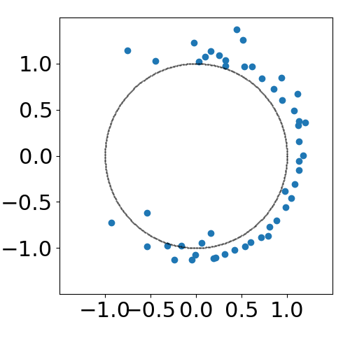
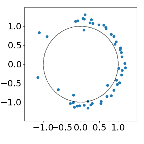
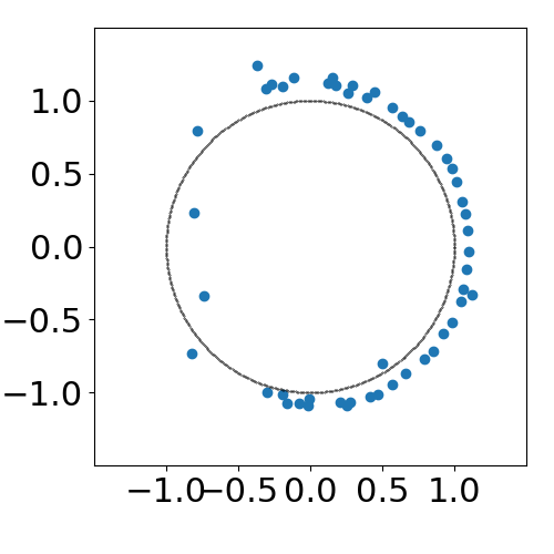
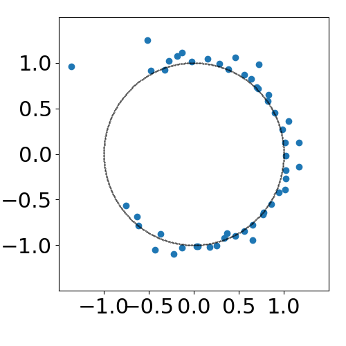
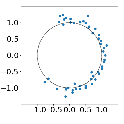
$j=1$	$j=2$	$j=3$	$j=4$	$j=5$

(a) Deep Koopman-layerd model

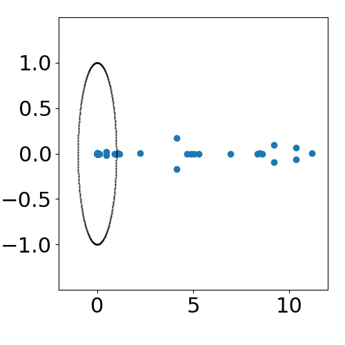
$j=1$	$j=2$	$j=3$	$j=4$	$j=5$

(b) EDMD

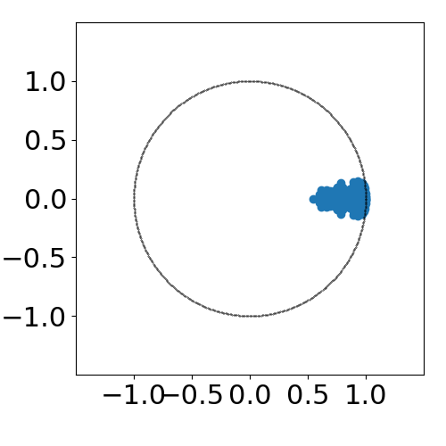
$j=1$	$j=2$	$j=3$	$j=4$	$j=5$

(c) KDMD

Figure 2: Eigenvalues of the estimated Koopman operators for the nonautonomous measure preserving system.

6.2.2 Damping oscillator with external force

Consider the nonautonomous dynamical system regarding a damping oscillator on a compact subspace of $\mathbb{R}$

$$\frac{\mathrm{d}^{2}x(t)}{\mathrm{d}t^{2}}=-\alpha\frac{\mathrm{d}x(t)}{\mathrm{d}t}-x(t)-a\sin(bt),$$ (7)

where $\alpha=0.1$, $a=b=1$. By setting $\mathrm{d}x/\mathrm{d}t$ as a new variable, we regard Eq. (7) as a first-ordered system on the two-dimensional space. We generated data, constructed the deep Koopman-layered model, and applied EDMD and KDMD for comparison in the same manner as Subsection 6.2.1. Figure 3 illustrates the results. In this case, since the dynamical system is not measure preserving, it is reasonable that the estimated Koopman operators have eigenvalues inside the unit circle. We can see that many eigenvalues for the deep Koopman-layered model are distributed inside the unit circle, and the distribution changes along the layers. Since the external force becomes large as $t$ becomes large, the damping effect becomes small as $t$ becomes large (corresponding to $j$ becoming large). Thus, the number of eigenvalues distributed inside the unit circle becomes small as $j$ becomes large. On the other hand, we cannot obtain this type of observation from the separate estimation of the Koopman operators by EDMD and KDMD.

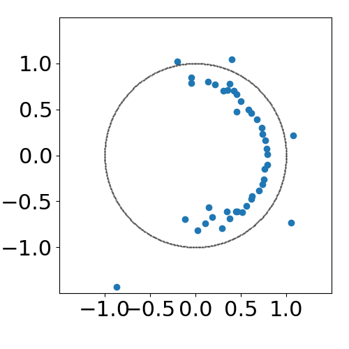
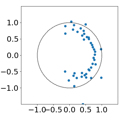
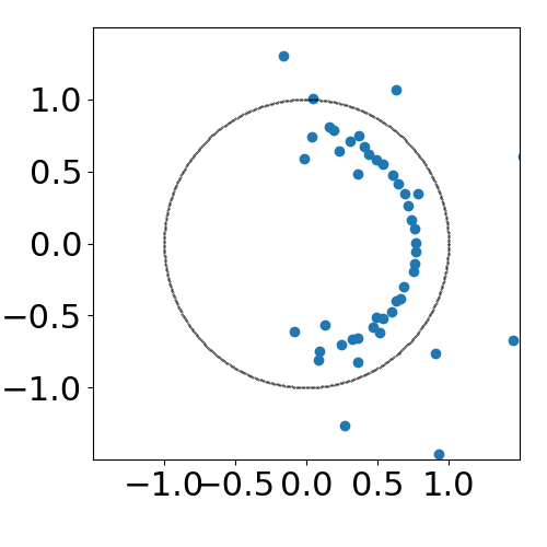
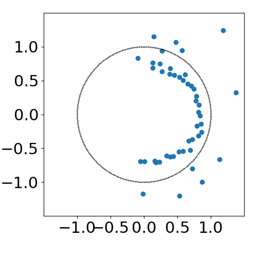
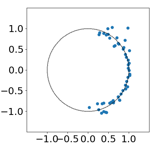
$j=1$	$j=2$	$j=3$	$j=4$	$j=5$

(a) Deep Koopman-layerd model

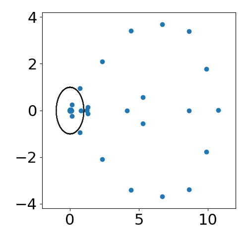
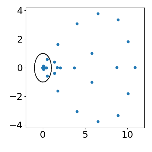
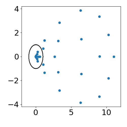
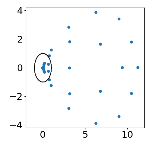
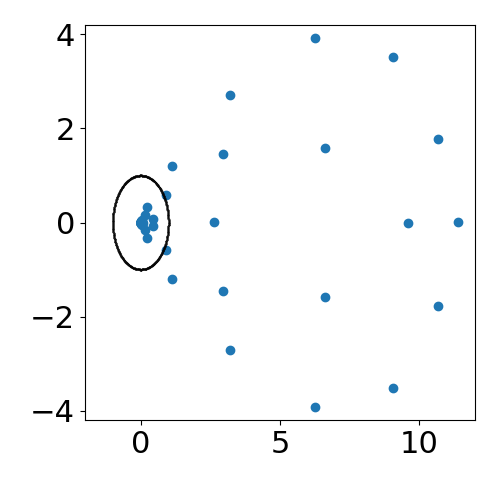
$j=1$	$j=2$	$j=3$	$j=4$	$j=5$

(b) EDMD

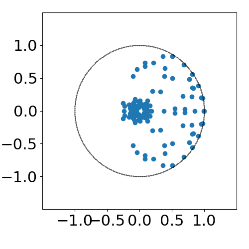
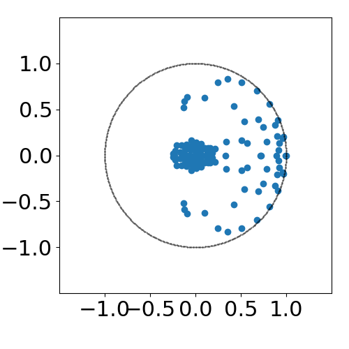
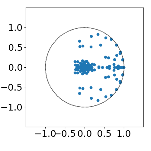
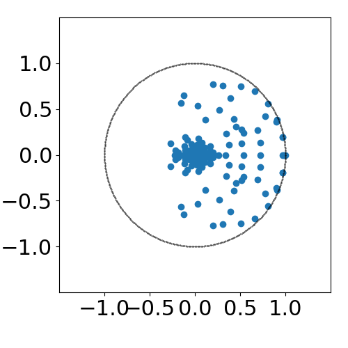
$j=1$	$j=2$	$j=3$	$j=4$	$j=5$

(c) KDMD

Figure 3: Eigenvalues of the estimated Koopman operators for the nonautonomous damping oscillator.

7 Connection with other methods

7.1 Deep Koopman-layered model as a neural ODE-based model

The model (1) can also be regarded as a model with multiple neural ODEs (Teshima et al., 2020b; Li et al., 2023, Section 3.3). From this perspective, we can also apply the model to standard tasks with ResNet. For existing Neural ODE-based models, we use numerical methods, such as Runge-Kutta methods, to solve the ODE (Chen et al., 2018). In our framework, solving the ODE corresponds to computing $\mathrm{e}^{\mathbf{L}_{j}}u$ for a matrix $\mathbf{L}_{j}$ and a vector $u$. As we stated in Subsection 3.2, we use Krylov subspace methods to compute $\mathrm{e}^{\mathbf{L}_{j}}u$. In this sense, our framework provides numerical linear algebraic way to train Neural ODE-based models by virtue of introducing Koopman generators and operators.

7.2 Connection with neural network-based Koopman approaches

In the framework of neural network-based Koopman approaches, we train an encoder $\phi$ and a decoder $\psi$ that minimizes $\|x_{t+1}-\psi(K\phi(x_{t}))\|$ for the given time-series $x_{0},x_{1},\ldots$ (Lusch et al., 2017; Azencot et al., 2020; Shi & Meng, 2022). Here, $K$ is a linear operator, and we can construct $K$ using EDMD or can train $K$ simultaneously with $\phi$ and $\psi$. For neural network-based Koopman approaches, since the encoder $\phi$ changes along the learning process, the representation space of the operator $K$ also changes. Thus, the theoretical analysis of these approaches is challenging. On the other hand, our deep Koopman-layered approach fixes the representation space using the Fourier functions and learns only the linear operators corresponding to Koopman generators by restricting the linear operator to a form based on the Koopman operator.

8 Conclusion and discussion

In this paper, we proposed deep Koopman-layered models based on the Koopman operator theory combined with Fourier functions and Toeplitz matrices. We showed that the Fourier basis forms a proper representation space of the Koopman operators in the sense of the universal and generalization property of the model. In addition to the theoretical solidness, the flexibility of the proposed model allows us to train the model to fit time-series data coming from nonautonomous dynamical systems.

According to Lemma 10 and Theorem 5, to represent any function, we need more than one Koopman layer. Investigating how many layers we need and how the representation power grows as the number of layers increases theoretically remains for future work. In addition, we applied Krylov subspace methods to approximate the actions of the Koopman operators to vectors. Since the Krylov subspace methods are iterative methods, we can control the accuracy of the approximation by controlling the iteration number. How to decide and change the iteration number throughout the learning process for more efficient computations is also future work.

Acknowledgements

We would like to thank Dr. Isao Ishikawa for a constructive discussion.

Appendix

Appendix A Proofs

We provide the proofs of statements in the main text.

Proposition 2    The $(n,l)$-entry of the representation matrix $Q_{N}^{*}L_{j}Q_{N}$ of the approximated operator is

$$\sum_{k=1}^{d}\sum_{n_{R_{j}}-l\in M^{j}_{R_{j}}}\sum_{n_{R_{j}-1}-n_{R_{j}}\in M^{j}_{R_{j}-1}}\cdots\sum_{n_{2}-n_{3}\in M^{j}_{2}}\sum_{n-n_{2}\in M^{j}_{1}}$$

$$\qquad\qquad\qquad\qquad a^{j,k}_{n_{R_{j}}-l,R_{j}}a^{j,k}_{n_{R_{j}-1}-n_{R_{j}},R_{j-1}}\cdots a^{j,k}_{n_{2}-n_{3},2}a^{j,k}_{n-n_{2},1}\mathrm{i}l_{k},$$

where $l_{k}$ is the $k$th element of the index $l\in\mathbb{Z}^{d}$. Moreover, we set $n_{r}=m_{R_{j}}+\cdots+m_{r}+l$, thus $n_{1}=n$, $m_{r}=n_{r}-n_{r+1}$ for $r=1,\ldots,R_{j}-1$, and $m_{R_{j}}=n_{R_{j}}-l$.

Proof  We have

$$\left\langle q_{n},L_{j}q_{l}\right\rangle =\bigg{\langle}q_{n},\sum_{k=1}^{d}\sum_{m_{R_{j}}\in M^{j}_{R_{j}}}a^{j,k}_{m_{R_{j}},R_{j}}q_{m_{R_{j}}}\cdots\sum_{m_{1}\in M^{j}_{1}}a^{j,k}_{m_{1},1}q_{m_{1}}\mathrm{i}l_{k}q_{l}\bigg{\rangle}$$

$$=\bigg{\langle}q_{n},\sum_{k=1}^{d}\sum_{m_{R_{j}}\in M^{j}_{R_{j}}}\cdots\sum_{m_{1}\in M^{j}_{1}}a^{j,k}_{m_{R_{j}},R_{j}}\cdots a^{j,k}_{m_{1},1}q_{m_{R_{j}}+\cdots+m_{1}+l}\mathrm{i}l_{k}\bigg{\rangle}$$

$$=\sum_{k=1}^{d}\sum_{\begin{subarray}{c}m_{R_{j}}+\cdots+m_{1}+l=n\\ m_{R_{j}}\in M^{j}_{R_{j}}\cdots m_{1}\in M^{j}_{1}\end{subarray}}a^{j,k}_{m_{R_{j}},R_{j}}\cdots a^{j,k}_{m_{1},1}\mathrm{i}l_{k}$$

$$=\sum_{k=1}^{d}\sum_{n_{R_{j}}-l\in M^{j}_{R_{j}}}\sum_{n_{R_{j}-1}-n_{R_{j}}\in M^{j}_{R_{j}-1}}\cdots\sum_{n_{2}-n_{3}\in M^{j}_{2}}\sum_{n-n_{2}\in M^{j}_{1}}$$

$$\qquad\qquad\qquad\qquad a^{j,k}_{n_{R_{j}}-l,R_{j}}a^{j,k}_{n_{R_{j}-1}-n_{R_{j}},R_{j-1}}\cdots a^{j,k}_{n_{2}-n_{3},2}a^{j,k}_{n-n_{2},1}\mathrm{i}l_{k}.$$

$\Box$

Corollary 6    Assume $v\in L_{0}^{2}(\mathbb{T}^{d})$ and $v\neq 0$. For any sequence $g_{1}(t_{1},\cdot),\ldots,g_{\tilde{J}}(t_{\tilde{J}},\cdot)$ of flows that satisfies $v\circ g_{\tilde{J}}(t_{\tilde{J}},\cdot)\circ\cdots\circ g_{j}(t_{j},\cdot)\in L^{2}_{0}(\mathbb{T}^{d})$ and $v\circ g_{\tilde{J}}(t_{\tilde{J}},\cdot)\circ\cdots\circ g_{j}(t_{j},\cdot)\neq 0$ for $j=1\ldots\tilde{J}$, and for any $\epsilon>0$, there exist a finite set $N\subset\mathbb{Z}\setminus\{0\}$, integers $0<J_{1}<\cdots<J_{\tilde{J}}$, and matrices $\mathbf{L}_{1},\ldots,\mathbf{L}_{J_{\tilde{J}}}\in T(N,\mathbb{C})$ such that $\|v\circ g_{\tilde{J}}(t_{\tilde{J}},\cdot)\circ\cdots\circ g_{j}(t_{j},\cdot)-\mathbf{G}_{j}\|\leq\epsilon$ and $\mathbf{G}_{j}=Q_{N}\mathrm{e}^{\mathbf{L}_{J_{j-1}+1}}\cdots\mathrm{e}^{\mathbf{L}_{J_{\tilde{J}}}}Q_{N}^{*}v$ for $j=1,\ldots,\tilde{J}$, where $J_{0}=1$.

Proof  Since $v\circ g_{\tilde{J}}(t_{\tilde{J}},\cdot)\circ\cdots\circ g_{j}(t_{j},\cdot)\in L^{2}_{0}(\mathbb{T}^{d})$ and $v\circ g_{\tilde{J}}(t_{\tilde{J}},\cdot)\circ\cdots\circ g_{j}(t_{j},\cdot)\neq 0$, there exist finite $N_{j}\subset\mathbb{Z}^{d}\setminus\{0\}$ and $\mathbf{G}_{j}\in V_{N_{j}}$, $\mathbf{G}_{j}\neq 0$ such that $\|v\circ g_{\tilde{J}}(t_{\tilde{J}},\cdot)\circ\cdots\circ g_{j}(t_{j},\cdot)-\mathbf{G}_{j}\|\leq\epsilon$ for $j=1,\ldots,\tilde{J}$. Since $v\in L_{0}^{2}(\mathbb{T}^{d})$ and $v\neq 0$, there exist finite $N_{\tilde{J}+1}\subset\mathbb{Z}^{d}\setminus\{0\}$ such that $Q_{N_{\tilde{J}+1}}^{*}v\neq 0$. Let $N=\bigcup_{j=1}^{\tilde{J}+1}N_{j}$. By Lemma 11, since $Q_{N}^{*}v\neq 0$, there exist $J_{\tilde{J}-1},J_{\tilde{J}}\in\mathbb{N}$ and $\mathbf{L}_{J_{\tilde{J}-1}+1},\ldots,\mathbf{L}_{J_{\tilde{J}}}\in T(N,\mathbb{C})$ such that $\mathbf{G}_{\tilde{J}}=Q_{N}\mathrm{e}^{\mathbf{L}_{J_{\tilde{J}-1}+1}}\cdots\mathrm{e}^{\mathbf{L}_{J_{\tilde{J}}}}Q_{N}^{*}v$. Since $\mathbf{G}_{\tilde{J}}\neq 0$, again by Lemma 11, there exist $J_{\tilde{J}-2}\in\mathbb{N}$ and $\mathbf{L}_{J_{\tilde{J}-2}+1},\ldots,\mathbf{L}_{J_{\tilde{J}-1}}\in T(N,\mathbb{C})$ such that $\mathbf{G}_{\tilde{J}-1}=Q_{N}\mathrm{e}^{\mathbf{L}_{J_{\tilde{J}-2}+1}}\cdots\mathrm{e}^{\mathbf{L}_{J_{\tilde{J}-1}}}\mathrm{e}^{\mathbf{L}_{J_{\tilde{J}-1}+1}}\cdots\mathrm{e}^{\mathbf{L}_{J_{1}}}Q_{N}^{*}v=Q_{N}\mathrm{e}^{\mathbf{L}_{J_{\tilde{J}-2}+1}}\cdots\mathrm{e}^{\mathbf{L}_{J_{\tilde{J}-1}}}Q_{N}^{*}\mathbf{G}_{\tilde{J}}$. We continue to apply Lemma 11 to obtain the result. $\Box$

Lemma 9    Assume $N\subset\mathbb{Z}^{d}\setminus\{0\}$. Then, we have $\mathbb{C}^{N\times N}=T(N,\mathbb{C})$.

Proof  We show $\mathbb{C}^{N\times N}\subseteq T(N,\mathbb{C})$. The inclusion $\mathbb{C}^{N\times N}\supseteq T(N,\mathbb{C})$ is trivial. Since $N\subset\mathbb{Z}^{d}\setminus\{0\}$, for any $n=[n_{1},\ldots,n_{d}]\in N$, there exists $k\in\{1,\ldots,d\}$ such that $\mathrm{i}n_{k}=(D_{k})_{n,n}\neq 0$. We denote by $k_{\operatorname{min}}(n)$ the minimal index $k\in\{1,\ldots,d\}$ that satisfies $(D_{k})_{n,n}\neq 0$. Let $B\in\mathbb{C}^{N\times N}$. We decompose $B$ as $B=B_{1}+\ldots+B_{d}$, where $(B_{k})_{:,n}=B_{:,n}$ if $k=k_{\operatorname{min}}(n)$ and $(B_{k})_{:,n}=\mathbf{0}$ otherwise. Here, $(B_{k})_{:,n}$ is the $n$th column of $B_{k}$. Then, we have $(B_{k})_{:,n}=\mathbf{0}$ if $(D_{k})_{n,n}=0$. Let $D_{k}^{+}$ be the diagonal matrix defined as $(D_{k}^{+})_{n,n}=1/(D_{k})_{n,n}$ if $(D_{k})_{n,n}\neq 0$ and $(D_{k}^{+})_{n,n}=0$ if $(D_{k})_{n,n}=0$. In addition, let $C_{k}=B_{k}D_{k}^{+}$. Then, we have $B=\sum_{k=1}^{d}C_{k}D_{k}$. Applying Propostion 8, we have $B\in T(N,\mathbb{C})$, and obtain $\mathbb{C}^{N\times N}\subseteq T(N,\mathbb{C})$. $\Box$

Lemma 11    For any $\mathbf{u},\mathbf{v}\in\mathbb{C}^{N}\setminus\{0\}$, there exists $A\in GL(N,\mathbb{C})$ such that $\mathbf{u}=A\mathbf{v}$.

Proof  Let $n_{0}\in N$ and let $B\in\mathbb{N\times N}$ be defined as $B_{n,:}=1/\|\mathbf{v}\|^{2}\mathbf{v}^{*}$ for $n=n_{0}$ and so that $B_{n,:}$ and $B_{m,:}$ becoming orthogonal if $n\neq m$. Then, the $n$th element of $B\mathbf{v}$ is $1$ for $n=n_{0}$ and is $0$ for $n\neq n_{0}$. Let $C\in\mathbb{N\times N}$ be defined as $C_{n,:}=\mathbf{u}$ for $n=n_{0}$ and so that $C_{n,:}$ and $C_{m,:}$ becoming orthogonal if $n\neq m$. Then, $B,C\in GL(N,\mathbb{C})$ and $CB\mathbf{v}=\mathbf{u}$. $\Box$

Lemma 13    We have

$$\hat{R}_{S}(\mathcal{G}_{N})\leq\frac{\alpha}{\sqrt{S}}\max_{j\in N}\mathrm{e}^{\tau\|j\|_{1}}\sup_{\mathbf{L}_{1},\ldots,\mathbf{L}_{J}\in T(N,\mathbb{C})}\|\mathrm{e}^{\mathbf{L}_{1}}\|\cdots\|\mathrm{e}^{\mathbf{L}_{J}}\|\,\|v\|,$$

where $\alpha=\sum_{j\in\mathbb{Z}^{d}}\mathrm{e}^{-2\tau\|j\|_{1}}$.

Proof 

$$\hat{R}_{S}(\mathcal{G}_{N}) =\frac{1}{S}\mathrm{E}\bigg{[}\sup_{\mathbf{G}\in\mathcal{G}_{N}}\sum_{s=1}^{S}\mathbf{G}(x_{s})\sigma_{s}\bigg{]}=\frac{1}{S}\mathrm{E}\bigg{[}\sup_{\mathbf{G}\in\mathcal{G}_{N}}\sum_{s=1}^{S}\iota_{N}\mathbf{G}(x_{s})\sigma_{s}\bigg{]}$$

$$=\frac{1}{S}\mathrm{E}\bigg{[}\sup_{\mathbf{G}\in\mathcal{G}_{N}}\bigg{\langle}\sum_{s=1}^{S}\sigma_{s}\phi(x_{s}),\iota_{N}\mathbf{G}\bigg{\rangle}\bigg{]}\leq\frac{1}{S}\sup_{\mathbf{G}\in\mathcal{G}_{N}}\|\iota_{N}\mathbf{G}\|_{\mathcal{H}_{K}}\bigg{(}\sum_{s=1}^{S}K(x_{s},x_{s})\bigg{)}^{1/2}$$

$$\leq\frac{\alpha}{\sqrt{S}}\sup_{\mathbf{G}\in\mathcal{G}_{N}}\|\iota_{N}\|\|\mathbf{G}\|_{L^{2}(\mathbb{T}^{d})}\leq\frac{\alpha}{\sqrt{S}}\max_{j\in N}\mathrm{e}^{\tau\|j\|_{1}}\sup_{\mathbf{L}_{1},\ldots,\mathbf{L}_{J}\in T(N,\mathbb{C})}\|Q_{N}\mathrm{e}^{\mathbf{L}_{1}}\cdots\mathrm{e}^{\mathbf{L}_{J}}Q_{N}^{*}v\|$$

$$\leq\frac{\alpha}{\sqrt{S}}\max_{j\in N}\mathrm{e}^{\tau\|j\|_{1}}\sup_{\mathbf{L}_{1},\ldots,\mathbf{L}_{J}\in T(N,\mathbb{C})}\|\mathrm{e}^{\mathbf{L}_{1}}\|\cdots\|\mathrm{e}^{\mathbf{L}_{J}}\|\,\|v\|,$$

where $\alpha=\sum_{j\in\mathbb{Z}^{d}}\mathrm{e}^{-2\tau\|j\|_{1}}$. $\Box$

References

- Azencot et al. (2020) Omri Azencot, N. Benjamin Erichson, Vanessa Lin, and Michael Mahoney. Forecasting sequential data using consistent Koopman autoencoders. In Proceedings of the 37th International Conference on Machine Learning (ICML), 2020.
- Bartlett et al. (2017) Peter L Bartlett, Dylan J Foster, and Matus J Telgarsky. Spectrally-normalized margin bounds for neural networks. In Proceedings of the 31st Conference on Neural Information Processing Systems (NIPS), 2017.
- Brunton & Kutz (2019) Steven L. Brunton and J. Nathan Kutz. Data-Driven Science and Engineering: Machine Learning, Dynamical Systems, and Control. Cambridge University Press, 2019.
- Budišić et al. (2012) Marko Budišić, Ryan Mohr, and Igor Mezić. Applied Koopmanism. Chaos (Woodbury, N.Y.), 22:047510, 2012.
- Chen et al. (2018) Ricky T. Q. Chen, Yulia Rubanova, Jesse Bettencourt, and David K Duvenaud. Neural ordinary differential equations. In Proceedings of the 32rd Conference on Neural Information Processing Systems (NeurIPS), 2018.
- Colbrook & Townsend (2024) Matthew J. Colbrook and Alex Townsend. Rigorous data-driven computation of spectral properties of Koopman operators for dynamical systems. Communications on Pure and Applied Mathematics, 77(1):221–283, 2024.
- Das et al. (2021) Suddhasattwa Das, Dimitrios Giannakis, and Joanna Slawinska. Reproducing kernel Hilbert space compactification of unitary evolution groups. Applied and Computational Harmonic Analysis, 54:75–136, 2021.
- Gallopoulos & Saad (1992) Efstratios Gallopoulos and Yousef Saad. Efficient solution of parabolic equations by Krylov approximation methods. SIAM Journal on Scientific and Statistical Computing, 13(5):1236–1264, 1992.
- Giannakis & Das (2020) Dimitrios Giannakis and Suddhasattwa Das. Extraction and prediction of coherent patterns in incompressible flows through space-time Koopman analysis. Physica D: Nonlinear Phenomena, 402:132211, 2020.
- Giannakis et al. (2022) Dimitrios Giannakis, Abbas Ourmazd, Philipp Pfeffer, Jörg Schumacher, and Joanna Slawinska. Embedding classical dynamics in a quantum computer. Physical Review A, 105(5):052404, 2022.
- Golowich et al. (2018) Noah Golowich, Alexander Rakhlin, and Ohad Shamir. Size-independent sample complexity of neural networks. In Proceedings of the 2018 Conference On Learning Theory (COLT), 2018.
- Güttel (2013) Stefan Güttel. Rational Krylov approximation of matrix functions: Numerical methods and optimal pole selection. GAMM-Mitteilungen, 36(1):8–31, 2013.
- Hall (2015) Brian C. Hall. Lie Groups, Lie Algebras, and Representations –An Elementary Introduction–. Springer, 2nd edition, 2015.
- Hashimoto & Nodera (2016) Yuka Hashimoto and Takashi Nodera. Inexact shift-invert Arnoldi method for evolution equations. ANZIAM Journal, 58:E1–E27, 2016.
- Hashimoto et al. (2020) Yuka Hashimoto, Isao Ishikawa, Masahiro Ikeda, Yoichi Matsuo, and Yoshinobu Kawahara. Krylov subspace method for nonlinear dynamical systems with random noise. Journal of Machine Learning Research, 21(172):1–29, 2020.
- Hashimoto et al. (2024) Yuka Hashimoto, Sho Sonoda, Isao Ishikawa, Atsushi Nitanda, and Taiji Suzuki. Koopman-based generalization bound: New aspect for full-rank weights. In Proceedings of the 12th International Conference on Learning Representations (ICLR), 2024.
- Ishikawa et al. (2018) Isao Ishikawa, Keisuke Fujii, Masahiro Ikeda, Yuka Hashimoto, and Yoshinobu Kawahara. Metric on nonlinear dynamical systems with Perron-Frobenius operators. In Proceedings of the 32nd Conference on Neural Information Processing Systems (NeurIPS), 2018.
- Ishikawa et al. (2024) Isao Ishikawa, Yuka Hashimoto, Masahiro Ikeda, and Yoshinobu Kawahara. Koopman operators with intrinsic observables in rigged reproducing kernel Hilbert spaces. arXiv:2403.02524, 2024.
- Kawahara (2016) Yoshinobu Kawahara. Dynamic mode decomposition with reproducing kernels for Koopman spectral analysis. In Proceedings of the 30th Conference on Neural Information Processing Systems (NIPS), 2016.
- Kingma & Ba (2015) Diederik P. Kingma and Jimmy Ba. Adam: A method for stochastic optimization. In Proceedings of the 3rd International Conference on Learning Representations (ICLR), 2015.
- Klus et al. (2020) Stefan Klus, Ingmar Schuster, and Krikamol Muandet. Eigendecompositions of transfer operators in reproducing kernel Hilbert spaces. Journal of Nonlinear Science, 30:283–315, 2020.
- Koopman (1931) Bernard Koopman. Hamiltonian systems and transformation in Hilbert space. Proceedings of the National Academy of Sciences, 17(5):315–318, 1931.
- Li et al. (2023) Qianxiao Li, Ting Lin, and Zuowei Shen. Deep learning via dynamical systems: An approximation perspective. Journal of the European Mathematical Society, 25(5):1671–1709, 2023.
- Liu et al. (2023) Yong Liu, Chenyu Li, Jianmin Wang, and Mingsheng Long. Koopa: Learning non-stationary time series dynamics with Koopman predictors. In Proceedings of the 37th Conference on Neural Information Processing Systems (NeurIPS), 2023.
- Lusch et al. (2017) Bethany Lusch, J. Nathan Kutz, and Steven L. Brunton. Deep learning for universal linear embeddings of nonlinear dynamics. Nature Communications, 9:4950, 2017.
- Maćešić et al. (2018) Senka Maćešić, Nelida Črnjarić Žic, and Igor Mezić. Koopman operator family spectrum for nonautonomous systems. SIAM Journal on Applied Dynamical Systems, 17(4):2478–2515, 2018.
- Mezić (2022) Igor Mezić. On numerical approximations of the Koopman operator. Mathematics, 10(7):1180, 2022.
- Mohri et al. (2012) Mehryar Mohri, Afshin Rostamizadeh, and Ameet Talwalkar. Foundations of Machine Learning. MIT press, 1st edition, 2012.
- Neyshabur et al. (2015) Behnam Neyshabur, Ryota Tomioka, and Nathan Srebro. Norm-based capacity control in neural networks. In Proceedings of the 2015 Conference on Learning Theory (COLT), 2015.
- Schmid (2022) Peter J. Schmid. Dynamic mode decomposition and its variants. Annual Review of Fluid Mechanics, 54:225–254, 2022.
- Shi & Meng (2022) Haojie Shi and Max Q.-H. Meng. Deep Koopman operator with control for nonlinear systems. IEEE Robotics and Automation Letters, 7(3):7700–7707, 2022.
- Teshima et al. (2020a) Takeshi Teshima, Isao Ishikawa, Koichi Tojo, Kenta Oono, Masahiro Ikeda, and Masashi Sugiyama. Coupling-based invertible neural networks are universal diffeomorphism approximators. In Proceedings of the 34th Conference on Neural Information Processing Systems (NeurIPS), 2020a.
- Teshima et al. (2020b) Takeshi Teshima, Koichi Tojo, Masahiro Ikeda, Isao Ishikawa, and Kenta Oono. Universal approximation property of neural ordinary differential equations. In NeurIPS 2020 Workshop on Differential Geometry meets Deep Learning, 2020b.
- Williams et al. (2015) Matthew O. Williams, Ioannis G. Kevrekidis, and Clarence W. Rowley. A data-driven approximation of the Koopman operator: extending dynamic mode decomposition. Journal of Nonlinear Science, 25:1307–1346, 2015.
- Xiong et al. (2024) Wei Xiong, Xiaomeng Huang, Ziyang Zhang, Ruixuan Deng, Pei Sun, and Yang Tian. Koopman neural operator as a mesh-free solver of non-linear partial differential equations. Journal of Computational Physics, 513:113194, 2024.
- Ye & Lim (2016) Ke Ye and Lek-Heng Lim. Every matrix is a product of Toeplitz matrices. Foundation of Computational Mathematics, 16:577–598, 2016.
- Yosida (1980) Kôsaku Yosida. Functional Analysis. Springer, 6th edition, 1980.