Contrasting dynamical properties of single-Q and triple-Q magnetic orderings in a triangular lattice antiferromagnet

Abstract

Multi-$\mathbf{Q}$ magnetic structures on triangular lattices, with their two-dimensional topological spin texture, have attracted significant interest. However, unambiguously confirming their formation by excluding the presence of three equally-populated single-$\mathbf{Q}$ domains remains challenging. In the metallic triangular lattice antiferromagnet Co1/3TaS2, two magnetic ground states have been suggested at different temperature ranges, with the low-temperature phase being a triple-$\mathbf{Q}$ structure corresponding to the highest-density Skyrmion lattice. Using inelastic neutron scattering (INS) and advanced spin dynamics simulations, we demonstrate a clear distinction in the excitation spectra between the single-${\mathbf{Q}}$ and triple-${\mathbf{Q}}$ phases of Co1/3TaS2 and, more generally, a triangular lattice. First, we refined the spin Hamiltonian by fitting the excitation spectra measured in its paramagnetic phase, allowing us to develop an unbiased model independent of magnetic ordering. Second, we observed that the two magnetically ordered phases in Co1/3TaS2 exhibit markedly different behaviors in their long-wavelength Goldstone modes. Our spin model, derived from the paramagnetic phase, confirms that these behaviors originate from the single-${\mathbf{Q}}$ and triple-${\mathbf{Q}}$ nature of the respective ordered phases, providing unequivocal evidence of the single-$\mathbf{Q}$ to triple-$\mathbf{Q}$ phase transition in Co1/3TaS2. Importantly, we propose that the observed contrast in the long-wavelength spin dynamics between the single-${\mathbf{Q}}$ and triple-${\mathbf{Q}}$ orderings is universal, offering a potentially unique way to distinguish a generic triple-$\mathbf{Q}$ ordering on a triangular lattice from its multi-domain single-${\mathbf{Q}}$ counterparts. Furthermore, we observe a sizable discrepancy between the measured and simulated magnon spectra exclusively at 5 K (a triple-$\mathbf{Q}$ phase), while there is a satisfactory agreement at 30 K (a single-$\mathbf{Q}$ phase). We conjecture that this discrepancy arises from magnon energy renormalization due to magnon-magnon interactions, which is order-of-magnitude enhanced during the single-$\mathbf{Q}$ to triple-$\mathbf{Q}$ transition because of the non-collinear configuration of the latter structure. Finally, we summarize our finding and describe its applicability, with examples of similar hexagonal systems forming potential triple-${\mathbf{Q}}$ orderings. This work represents a rare experimental success in systematically contrasting the characteristic dynamical property of single-${\mathbf{Q}}$ and the triple-${\mathbf{Q}}$ phases on triangular lattices. With the identification of the triple-$\mathbf{Q}$ order in the intercalated van der Waals (vdW) system, it also highlights the potential of vdW materials in studying two-dimensional topological spin texture.

I Introduction

Symmetry and topology are central themes in modern magnetism, with antiferromagnetism gaining increasing recognition for its potential in these areas. The diverse configurations of antiferromagnetic spins give rise to various combinations of magnetic symmetry and topological properties, each capable of producing unique phenomena [1, 2]. Since diffraction techniques are commonly used to reveal the structure of antiferromagnetic textures, these textures are often characterized by their Fourier components ${\mathbf{S}}_{\mathbf{Q}}$, where their magnitudes $|{\mathbf{S}}_{\mathbf{Q}}|^{2}$ correspond to Bragg peak intensities. Complex spin textures typically involve multiple Bragg peaks located at symmetry-related wave vectors ${\mathbf{Q}}_{\nu}$, generally referred to as multi-${\mathbf{Q}}$ orderings.

Recent studies on various antiferromagnetic orders have renewed interest in multi-${\mathbf{Q}}$ magnetic orderings. Notably, these orderings can give rise to topologically non-trivial spin textures, such as skyrmion, meron, or vortex crystals [3, 4, 5, 6, 7, 8, 9, 10, 11, 12]. Among them, magnetic skyrmions are a representative example of two-dimensional (2D) topological spin textures, where the spins twist in a manner that wraps around the Bloch sphere [13, 14]. The integer topological invariant, or skyrmion charge $Q_{\rm Skx}$, corresponds to the number of times the spin texture wraps the Bloch sphere. Due to the conservation of this charge under continuous deformations, skyrmions behave as emergent mesoscale particles, potentially playing a crucial role in future spintronic memory devices [14, 15, 16, 17]. However, identifying such multi-${\mathbf{Q}}$ orderings experimentally can be challenging, often requiring specialized techniques beyond conventional diffraction to probe key aspects of their structure.

Hexagonal 2D structures provide ideal platforms for stabilizing triple-$\mathbf{Q}$ skyrmion, meron, or vortex crystals, as the sum of the three ordering wave vectors ${\mathbf{Q}}_{1}$, ${\mathbf{Q}}_{2}$ and ${\mathbf{Q}}_{3}$ related by the three-fold symmetry equals zero: ${\mathbf{Q}}_{1}+{\mathbf{Q}}_{2}+{\mathbf{Q}}_{3}={\mathbf{0}}$. For generic values of $|{\mathbf{Q}}_{\nu}|$, multi-${\mathbf{Q}}$ magnetic orderings are always accompanied by higher harmonics to fulfil the constraint $|{\mathbf{S}}_{j}|=S$ of fixed spin length across all sites ($j$) in real space. However, generating higher harmonics is penalized by isotropic exchange interactions as their Fourier-transform $J({\mathbf{q}})$ has global minima at the ordering wave vectors ${\mathbf{q}}={\mathbf{Q}}_{\nu}$. In other words, except for very particular values of $|{\mathbf{Q}}_{\nu}|$, single-${\mathbf{Q}}$ magnetic orderings are favored by Heisenberg interactions, necessitating additional terms–such as the Zeeman coupling to external fields or anisotropic single-ion or exchange terms–to stabilize multi-${\mathbf{Q}}$ structures. The advantage of hexagonal systems is that since ${\mathbf{Q}}_{1}+{\mathbf{Q}}_{2}+{\mathbf{Q}}_{3}={\mathbf{0}}$, the first harmonic generated by the superposition of the two symmetry-related ordering wave vectors is the remaining third ordering wave vector, i.e., ${\mathbf{Q}}_{\mu}+{\mathbf{Q}}_{\nu}=-|\epsilon_{\mu\nu\eta}|{\mathbf{Q}}_{\eta}$, where $\epsilon_{\mu\nu\eta}$ is the Levi-Civita symbol. Thus, this harmonic is not penalized by the Heisenberg exchange interactions.

As the simplest hexagonal structure capable of hosting magnetic skyrmion, meron, or vortex crystals, triangular lattices have been frequently utilized to study multi-$\mathbf{Q}$ magnetic orderings [3, 4, 5, 7, 18, 8, 19, 20, 11, 10, 12]. However, even for these relatively simple lattice structures, it remains challenging how one can experimentally distinguish between a triple-${\mathbf{Q}}$ magnetic ordering and the superposition of multiple single-${\mathbf{Q}}$ domains. Since the three ${\mathbf{Q}}_{\nu}$ vectors in a triple-${\mathbf{Q}}$ magnetic ordering are related by the three-fold rotational symmetry of the triangular lattice, both single-${\mathbf{Q}}$ and triple-${\mathbf{Q}}$ orderings produce a similar hexagonal pattern of magnetic Bragg peaks with equal intensities in their neutron diffraction experiments. As a result, identifying triple-${\mathbf{Q}}$ magnetic structures requires advanced experimental tools to distinguish them from alternative scenarios involving three equally-populated domains of single-${\mathbf{Q}}$ or double-${\mathbf{Q}}$ spin configurations, which spontaneously break the C₃ lattice symmetry.

While various advanced techniques have successfully confirmed triple-${\mathbf{Q}}$ magnetic structures in several systems [21, 22, 23], a promising approach for addressing this challenge is to complement diffraction measurements with inelastic neutron scattering (INS), which captures the collective modes (magnons) of each magnetic ordering. Due to their distinct spin configurations, triple-${\mathbf{Q}}$ and single-${\mathbf{Q}}$ magnetic orderings are expected to exhibit different magnetic excitation spectra. This perspective has been suggested by previous studies [24], but a systematic experimental comparison of spin dynamics between these two types of orderings is still lacking. In particular, it would be valuable to clarify the characteristic dynamical properties of each phase, independent of specific conditions, as this could greatly aid in distinguishing between single-${\mathbf{Q}}$ and triple-${\mathbf{Q}}$ orderings. Ideally, this could be experimentally addressed using a system that exhibits both single-${\mathbf{Q}}$ and triple-${\mathbf{Q}}$ magnetic orderings as external variables (e.g., temperature) are varied. This would allow for a direct comparison of their dynamical characteristics under the same spin Hamiltonian, which is the main object of this work.

The layered metallic triangular lattice antiferromagnet Co1/3TaS2 has recently gained attention due to its unique non-coplanar triple-${\mathbf{Q}}$ magnetic ground state. Co1/3TaS2 undergoes two antiferromagnetic phase transitions at $T_{\mathrm{N}1}$ = 38 K and $T_{\mathrm{N}2}$ = 26.5 K [Fig. 1(a)], and neutron diffraction measurements revealed that both phases develop magnetic Bragg peaks on the M points of the Brillouin zone [i.e., $\mathbf{Q}_{\nu}=\mathbf{G}_{\nu}/2$ with $\nu=1,2,3$, where $\mathbf{G}_{\nu}$ are reciprocal lattice vectors related by 120 degree rotations about the $c$-axis] [25, 26]. However, the observation of a large spontaneous Hall conductivity $\sigma_{xy}(\mathbf{H}=0)$ below $T_{\mathrm{N}2}$ rules out the possibility of a multi-domain single-${\mathbf{Q}}$ scenario for $T<T_{\mathrm{N2}}$: such a quantity is strictly forbidden under a single-${\mathbf{Q}}$ long-range order with $\mathbf{Q}_{\nu}=\mathbf{G}_{\nu}/2$, due to the symmetry of time reversal combined with the translation of a lattice vector ($\tau_{1a}T$) [25, 26]. Consequently, the presence of triple-${\mathbf{Q}}$ ordering below $T_{\mathrm{N}2}$ has been confirmed through a combination of neutron diffraction and bulk electrical transport measurement, which can together determine the symmetry of the magnetic ordering. In addition, the potential for obtaining atomically-thin flakes of Co1/3TaS2 via mechanical exfoliation [27] or chemical intercalation [28, 29] highlights its promise as a platform for exploring the genuine 2D limit of triple-${\mathbf{Q}}$ magnetism exhibiting topologically nontrivial spin textures.

The fundamental importance of this commensurate triple-${\mathbf{Q}}$ ordering merits more explanation. This ordering only consists of four sublattices pointing along the principal directions of a regular tetrahedron [Fig. 1(c)], thereby referred to as the tetrahedral triple-${\mathbf{Q}}$ ordering [30, 25]. Notably, alongside two-sublattice stripe and three-sublattice 120^∘ magnetic orderings, it is one of the three fundamental antiferromagnetic configurations in a triangular lattice system [25]. Moreover, this spin configuration is the highest density limit of a skyrmion lattice, sharing the same topological characteristics as skyrmions despite lacking a continuous real-space texture [12, 25]. The dense real-space Berry curvature owing to its small Skyrmion radius can indeed result in a substantial topological Hall effect (THE), explaining the observed spontaneous Hall effect in Co1/3TaS2 ($\rho_{xy}\sim 4\,\mu\Omega\,\mathrm{cm}$, or $\sigma_{xy}\sim 70\,\Omega^{-1}\mathrm{cm}^{-1}$) [27, 26] that is a few orders of magnitude larger than that observed in typical Skyrmion crystals, such as FeGe [31] and MnSi [32].

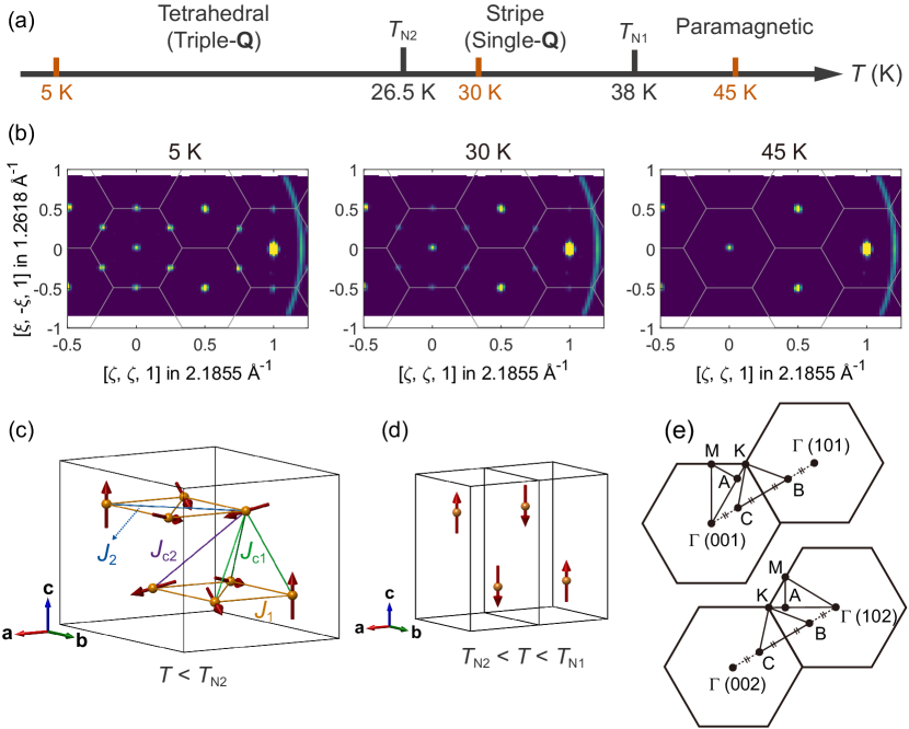
Figure 1: Basic information on the magnetism in Co1/3TaS2. (a) Schematic temperature-dependent phase diagram of Co1/3TaS2 as suggested by neutron diffraction and transport measurements [25, 26]. The three orange vertical ticks indicate the temperatures at which the INS data were collected. (b) Elastic component ($-0.52\,\mathrm{meV}<E<0.52\,\mathrm{meV})$ of the single-crystal INS data ($E_{i}=13\,\mathrm{meV}$) at 5 K ($T<T_{\mathrm{N2}}$), 30 K ($T_{\mathrm{N2}}<T<T_{\mathrm{N1}}$), and 45 K ($T_{\mathrm{N}1}$ $<T$). (c)–(d) Tetrahedral triple-${\mathbf{Q}}$ and stripe single-${\mathbf{Q}}$ magnetic ground states at $T<T_{\mathrm{N2}}$ and $T_{\mathrm{N2}}<T<T_{\mathrm{N1}}$, respectively [25, 26]. The exchange interaction paths considered in this work are illustrated in (c). (e) Brillouin zones on [$H$, $K$, 1] and [$H$, $K$, 2] planes. Labels of high-symmetry ${\mathbf{q}}$ points and corresponding high-symmetry contours used throughout this work are also plotted.

Another significant observation in Co1/3TaS2 relevant to this study is the presence of an intermediate phase between the tetrahedral triple-${\mathbf{Q}}$ ($T<T_{\mathrm{N2}}$) and the paramagnetic phase ($T>T_{\mathrm{N1}}$). This intermediate phase is characterized by zero $\sigma_{xy}(\mathbf{H}=0)$ and $M_{z}(\mathbf{H}=0)$, and Co²⁺ magnetic moments are aligned along the out-of-plane direction according to neutron diffraction results [25, 26]. Based on these findings, previous studies have suggested that the intermediate phase likely corresponds to a stripe single-${\mathbf{Q}}$ ordering [Fig. 1(a) and 1(d)] [25, 26]. Together with the low-temperature (low-$T$) triple-${\mathbf{Q}}$ phase, this intermediate phase can be reproduced using a simple model Hamiltonian with small isotropic four-spin interactions, breaking the accidental degeneracy between the stripe single-${\mathbf{Q}}$ and tetrahedral triple-${\mathbf{Q}}$ orderings present in the pure Heisenberg model (see Section III. A) [25].

Therefore, Co1/3TaS2 would provide a rare ideal system for studying the dynamics of both single-${\mathbf{Q}}$ and triple-${\mathbf{Q}}$ magnetic orderings within the same spin Hamiltonian, simply by adjusting the temperature [Fig. 1(a)]. Notably, modelling the spin dynamics of temperature-dependent magnetic structures can be accomplished by combining Landau-Lifshitz dynamics (LLD) simulations with a recently-developed technique that accounts for the renormalization of the classical dynamics due to quantum effects. This latest theoretical approach has proven successful in describing experimental inelastic neutron scattering (INS) data measured at finite temperatures [33, 34, 35, 36].

In this article, we present a comprehensive study on the spin dynamics of Co1/3TaS2, unambiguously identifying the stripe single-${\mathbf{Q}}$ and tetrahedral triple-${\mathbf{Q}}$ orderings in Co1/3TaS2 and highlighting the distinctive dynamical properties of each. Through INS measurements and theoretical calculations, we analyzed the magnetic excitation spectra of the paramagnetic phase ($T>T_{\mathrm{N1}}$) and the two ordered phases ($T_{\mathrm{N2}}<T<T_{\mathrm{N1}}$ and $T<T_{\mathrm{N2}}$) in single-crystal Co1/3TaS2. The core achievement of this work is the successful determination of bilinear exchange parameters by fitting dynamical spin structure factor maps [$S(\mathbf{q},\omega)$] of paramagnetic Co1/3TaS2, utilizing our state-of-the-art LLD simulation protocol (see Methods) and Bayesian optimization algorithm. This analysis allows us to obtain the optimal exchange parameter set independently of the magnetic ordering information, enabling a fair comparison of the single-$\mathbf{Q}$ and triple-$\mathbf{Q}$ spin dynamics based on the same Hamiltonian.

Most importantly, we present the distinct long-wavelength spin dynamics of the two ordered phases in Co1/3TaS2. While the intermediate phase ($T_{\mathrm{N2}}<T<T_{\mathrm{N1}}$) exhibits anisotropic velocity in the linear magnon modes along the principal in-plane momentum directions, these velocities become nearly isotropic at $T<T_{\mathrm{N2}}$. The LLD simulations based on our optimal spin model demonstrate that these observations can only be explained by the tetrahedral triple-${\mathbf{Q}}$ and stripe single-${\mathbf{Q}}$ phases, thereby unequivocally confirming the triple-${\mathbf{Q}}$ (single-${\mathbf{Q}}$) magnetic ground state at $T<T_{\mathrm{N2}}$ ($T_{\mathrm{N2}}<T<T_{\mathrm{N1}}$).

We further extend our analysis of the magnon velocities to more general sets of exchange parameters and suggest that anisotropic (nearly isotropic) velocities are likely characteristic dynamical properties of single-${\mathbf{Q}}$ (triple-${\mathbf{Q}}$) orderings. Since this insight is derived from a long-wavelength analysis of the models, it can be applied to distinguish between single-${\mathbf{Q}}$ and triple-${\mathbf{Q}}$ magnetic structures in hexagonal materials more broadly.

The final key observation we report is the presence of magnon linewidth broadening and energy renormalization in Co1/3TaS2. Notably, our comparison between experimental data and LLD simulations based on our optimal parameter set reveals that the latter feature is significantly enhanced in the tetrahedral triple-${\mathbf{Q}}$ phase ($T<T_{\mathrm{N2}}$). We provide a plausible interpretation on this result based on the magnon-magnon interactions, which are substantially enhanced in a non-collinear magnetic ground state. This distinction further contrasts the spin dynamics of the tetrahedral triple-${\mathbf{Q}}$ and stripe single-${\mathbf{Q}}$ phases, as only the former exhibits non-collinearity.

The paper is organized as follows: after the Methods section (Section II), we first introduce our effective spin Hamiltonian for Co1/3TaS2, along with its corresponding magnetic ground states and low-energy spin dynamics (Section III. A). Second, we describe our analysis of the paramagnetic spin dynamics, where we determine the strength of multiple bilinear interaction terms and validate their reliability through various means (Section III. B). We then present the experimental and theoretical spin wave spectra of the low-$T$ ($T<T_{\mathrm{N2}}$) and intermediate ($T_{\mathrm{N2}}<T<T_{\mathrm{N1}}$) phases in the long-wavelength limit, highlighting key features that allow us to distinguish between the triple-${\mathbf{Q}}$ and single-${\mathbf{Q}}$ orderings (Section III. C). In this section, we also argue that a nearly-isotropic (highly-anisotropic) dispersion of the low-energy magnon modes is the characteristic dynamical property of the triple-${\mathbf{Q}}$ (single-${\mathbf{Q}}$) phase. Fourth, we extend the analysis to full magnon spectra beyond the long-wavelength limit, revealing a more pronounced discrepancy between the data and the semi-classical LLD calculations in the low-$T$ triple-${\mathbf{Q}}$ phase, alongside a theoretical interpretation based on magnon-magnon interactions (Section III. D). Finally, in Section IV, we summarize our generalized protocol for distinguishing between single-${\mathbf{Q}}$ and triple-${\mathbf{Q}}$ orderings using INS and discuss its potential applications to other intriguing materials similar to Co1/3TaS2 or general two-dimensional magnets. We also provide remarks on our scenario of magnon-magnon interactions in the triple-${\mathbf{Q}}$ phase of Co1/3TaS2 and consider the validity and limitations of our isotropic spin Hamiltonian.

II Methods

Single-crystal Co1/3TaS2 was synthesized following the recipes described in Refs. [27, 25, 37]. The obtained crystals were meticulously characterized by measuring the temperature-dependent magnetization along the $c$-axis, which serves as a reliable indicator of Co composition [37]. Notably, only samples exhibiting $T_{\mathrm{N}2}$ = 26.5 K were selected for the measurements in this study, ensuring high quality with minimal Co vacancies [37]: this transition temperature is sensitive to the exact amount of Co compositions. Using CYTOP (CTL-809M, Asahi Glass, Japan), a total of 172 single-crystal Co1/3TaS2 pieces (12.05 g) were co-aligned on multiple aluminum plates, achieving a mosaicity within approximately 2^∘. The co-aligned assembly was oriented in the $(HHL)$-horizontal geometry (see Fig. 7 in Appendix). A sample holder without Co1/3TaS2 crystals was also prepared to measure background signals, independently.

INS data were collected at the 4SEASONS time-of-flight spectrometer at J-PARC, Japan [38]. Using the repetition-rate-multiplication (RRM) technique [39], we simultaneously collected data from multiple incident neutron energies: 46.7, 22.0, 12.8, 8.3, and 5.8 meV from a chopper frequency of 200 Hz. Data were acquired at 5, 30, and 45 K, with azimuthal sample rotation over 160^∘, and symmetrized according to the symmetry operations of the Co1/3TaS2 crystal structure. We used the Horace [40] and Utsusemi [41] software packages to analyze and visualize four-dimensional $S(\mathbf{q},\omega)$ maps. Background estimation was conducted by measuring the empty sample holder under identical conditions. Unless otherwise specified, the INS data are shown in this work after background subtraction.

Magnon dispersion [$\omega(\mathbf{q})$] and energy- and momentum-resolved $S(\mathbf{q},\omega)$ without temperature effects were calculated using the linear spin-wave theory (LSWT) within the SpinW [42] software package. Energy and momentum-resolved $S(\mathbf{q},\omega)$ at finite temperatures were calculated by the LLD simulations of a spin system, using the su(n)ny package [43, 44]. Renormalization of the scalar bi-quadratic interaction term from higher-order 1/$S$ corrections was applied based on the description in Ref. [45] (or see Appendix B). In our LLD simulations, a temperature-dependent renormalization scheme for the spin length was used, which allows for accurate simulations of magnetic excitation energies even under sizable thermal fluctuations. Further details on this treatment are provided in Refs. [33, 36].

For the calculations of $S(\mathbf{q},\omega)$ at 45 K ($T>T_{\mathrm{N1}}$), we simulated the time evolution of a Co1/3TaS2 supercell of size $24\times 24\times 16$ (18432 Co sites) using a Langevin time step ($\mathrm{d}t$) and a damping constant of 0.02 meV^-1 and 0.1, respectively. An initial equilibration phase ($t_{\mathrm{eq}}$) was performed for 4000 Langevin timesteps. The resulting $S(\mathbf{q},\omega)$ was averaged over 4 supercell replicas. For the simulations at 5 and 30 K, we used a larger supercell size of $30\times 30\times 24$, with $\mathrm{d}t=0.025$ meV^-1 and $t_{\mathrm{eq}}=10000$ time steps. In this case, $S(\mathbf{q},\omega)$ was averaged over 30 independent replicas to ensure an equal population of multiple magnetic domains: three magnetic domains related by a three-fold rotation about the $c$-axis for the single-${\mathbf{Q}}$ ordering, and two magnetic domains with opposite signs of scalar spin chirality for the triple-${\mathbf{Q}}$ ordering.

The resultant $S(\mathbf{q},\omega)$ was multiplied by the neutron polarization factor and the magnetic form factor of Co²⁺. It was then convolved with the instrumental energy and momentum resolutions, each derived from the geometry of 4SEASONS spectrometer and the full width at half-maximum (FWHM) of the (1/2, 0, 1) magnetic Bragg peak along the [$H$, 0, 0], [$-K$, 2$K$, 0], and [0, 0, $L$] directions, respectively. The effects of finite integration range perpendicular to the plotting axes of $S(\mathbf{q},\omega)$ slices were incorporated into the simulations by accounting for the same pixel histogram as the experimental $S(\mathbf{q},\omega)$ slices. Unless noted otherwise, all simulation results presented in this work include the aforementioned treatments.

III Results

III.1 Model Hamiltonian and its low-energy excitations

Previous studies have suggested that Co1/3TaS2 undergoes two magnetic phase transitions at $T_{\mathrm{N}2}$ and $T_{\mathrm{N}1}$ [Fig. 1(a)], leading to the formation of stripe single-${\mathbf{Q}}$ and tetrahedral triple-${\mathbf{Q}}$ magnetic orderings, as depicted in Fig. 1(c)–(d) [25, 26]. This two-step phase transition can be modelled using the following phenomenological spin Hamiltonian including Heisenberg and scalar biquadratic interactions [25] :

$$\mathcal{\hat{H}}=\mathcal{\hat{H}}_{\rm Heis}+\mathcal{\hat{H}}_{\rm Bq}$$ (1)

with

$$\mathcal{\hat{H}}_{\rm Heis} = \frac{1}{2}\sum_{\begin{subarray}{c}{\mathbf{r}},{\bm{\delta}}\\ a,b\end{subarray}}J^{ab}_{\bm{\delta}}\hat{\mathbf{S}}^{a}_{\mathbf{r}}\cdot\hat{\mathbf{S}}^{b}_{{\mathbf{r}}+{\bm{\delta}}},$$

$$\mathcal{\hat{H}}_{\rm Bq} = \frac{K}{2}\sum_{{\mathbf{r}},{\bm{\delta}}_{1},a}(\hat{\mathbf{S}}^{a}_{\mathbf{r}}\cdot\hat{\mathbf{S}}^{a}_{{\mathbf{r}}+{\bm{\delta}}_{1}})^{2},$$ (2)

where ${\bm{\delta}}$ runs over the position vectors of each unit cell, expressed in the basis of primitive vectors $\{{\mathbf{a}},{\mathbf{b}},{\mathbf{c}}\}$ shown in Fig. 1(c), when the origin is at the unit cell ${\mathbf{r}}$ and $a,b\in\{o,e\}$ run over the two Co sublattices corresponding to even and odd Co-layers. The factor of $1/2$ is included to avoid double-counting of each exchange interaction (each bond is shared between two sites). Finally, ${\bm{\delta}}_{1}$ runs only over nearest-neighbor sites on the same layer.

First, to describe magnetic orderings with wave vectors $\mathbf{Q}_{\nu}=\mathbf{G}_{\nu}/2$ [see Fig. 1(b)], it is convenient to Fourier transform the Heisenberg term:

$$\mathcal{\hat{H}}_{\rm Heis}=\sum_{\mathbf{Q},a,b}\tilde{J}^{ab}_{\mathbf{q}}\tilde{\mathbf{S}}^{a}_{\mathbf{Q}}\cdot\tilde{\mathbf{S}}^{b}_{\bar{\mathbf{Q}}},$$ (3)

with $\bar{\mathbf{Q}}\equiv-\mathbf{Q}$,

$$\tilde{\mathbf{S}}^{a}_{\mathbf{Q}}=\frac{1}{\sqrt{N}}\sum_{\mathbf{r}}e^{-i\mathbf{Q}\cdot{\mathbf{r}}}\mathbf{S}^{a}_{\mathbf{r}},$$ (4)

$N$ is the number of unit cells and the Fourier-transformed interaction matrix is given by

$$\tilde{J}^{ab}_{\mathbf{q}}\equiv\frac{1}{2}\sum_{\bm{\delta}}J^{ab}_{\bm{\delta}}e^{-i\mathbf{q}\cdot\bm{\delta}}.$$ (5)

Notably, to ensure $\mathbf{Q}_{\nu}=\mathbf{G}_{\nu}/2$, $\tilde{J}^{ab}_{\mathbf{q}}$ should possess its global minimum in the $\mathbf{q}$-space at $\mathbf{q}=\mathbf{G}_{\nu}/2$ (at the M points). The Fourier components obey the sum rule

$$\sum_{\mathbf{q}}\tilde{\mathbf{S}}^{a}_{\mathbf{q}}\cdot\tilde{\mathbf{S}}^{a}_{-\mathbf{q}}=N{\mathbf{S}}\cdot{\mathbf{S}},$$ (6)

that arises from the real space Casimir invariant ${\mathbf{S}}_{\mathbf{r}}\cdot{\mathbf{S}}_{\mathbf{r}}=S(S+1)$, which becomes $S^{2}$ in the classical limit ($S\to\infty$).

For the two Co sublattices configuring a hexagonal close packed stacking [see Fig. 1(c)], antiferromagnetic exchange interactions between even and odd layers [25] guarantees that a spin configuration of each layer conincides with the other after being translated along the vector $\mathbf{t}=(1,1,1/2)$. Thus, the vector amplitudes on even and odd sublattices are related in the following simple expression:

$$\tilde{\mathbf{S}}^{o}_{\mathbf{Q}_{\nu}}=e^{i{\bf Q}_{\nu}\cdot{\mathbf{t}}}\,\tilde{\mathbf{S}}^{e}_{\mathbf{Q}_{\nu}}.$$ (7)

However, when only the Heisenberg interactions are present, the stripe single-${\mathbf{Q}}$ and tetrahedral triple-${\mathbf{Q}}$ orderings remain accidentally degenerate. More generally, the single-$\mathbf{Q}$ ordering has exactly the same energy as any multi-$\mathbf{Q}$ ordering of the form:

$$\tilde{\mathbf{S}}^{a}_{\mathbf{q}}=\tilde{\mathbf{S}}^{a}_{\mathbf{Q}_{1}}\delta_{\mathbf{q},\mathbf{Q}_{1}}+\tilde{\mathbf{S}}^{a}_{\mathbf{Q}_{2}}\delta_{\mathbf{q},\mathbf{Q}_{2}}+\tilde{\mathbf{S}}^{a}_{\mathbf{Q}_{3}}\delta_{\mathbf{q},\mathbf{Q}_{3}},$$ (8)

where $\mathbf{Q}_{\nu}=\mathbf{G}_{\nu}/2$ ($\nu=1,2,3$). The three vector amplitudes $\mathbf{S}_{\mathbf{Q}_{\nu}}$ ($\nu=1,2,3$) are mutually orthogonal and obey the normalization condition (6)

$$|\tilde{\mathbf{S}}^{a}_{\mathbf{Q}_{1}}|^{2}+|\tilde{\mathbf{S}}^{a}_{\mathbf{Q}_{2}}|^{2}+|\tilde{\mathbf{S}}^{a}_{\mathbf{Q}_{3}}|^{2}=NS^{2}.$$ (9)

Notably, despite this degeneracy, the single-${\mathbf{Q}}$ phase becomes the true ground state at any $T>0$ since thermal fluctuations favor a collinear magnetic order [46, 47]. Thus, it is necessary to consider four-spin interactions to realize the tetrahedral triple-${\mathbf{Q}}$ ground state within the spin Hamiltonian framework. The scalar biquadratic interaction in Eq. 1 with $K>$ 0 is the simplest example of such. Yet it is important to note that other forms of four-spin interactions (e.g. see Ref. [48]) should also be considered to develop a complete spin model, although they are often omitted in experimental studies due to the extensive number of interaction coefficients that largely complicates the analysis.

While $K>0$ indeed favors the noncollinear tetrahedral ordering at $T=0$, the collinear single-${\mathbf{Q}}$ ordering can still emerge as a ground state at finite temperatures due to an order-by-thermal-disorder mechanism [46, 47]. Thus, tuning the magnitude of $K$ controls the presence and position of the single-${\mathbf{Q}}$ to triple-${\mathbf{Q}}$ transition at $T=$ $T_{\mathrm{N}2}$ [Fig. 1(a)] [25]. Our choice of $K\sim 0.06J_{1}$ reproduces $T_{\mathrm{N}2}$/$T_{\mathrm{N}1}$ $\sim 0.7$ observed in Co1/3TaS2, where the higher-order renormalization for the biquadratic term is considered (see Appendix B).

For the long-wavelength limit, we introduce the relative coordinate ${\mathbf{k}}=\mathbf{q}-\mathbf{Q}_{\nu}$ with $|{\mathbf{k}}|\ll 1$, which measures a deviation from the ordering wave vector. In this limit, both the three-domain single-$\mathbf{Q}$ and single-domain triple-$\mathbf{Q}$ phase result in the universal profile of magnons consisting of linear and quadratic dispersion. We will use subscripts “$s$” and “$t$” to indicate the low-energy dispersions of the single domain single-$\mathbf{Q}$ and triple-$\mathbf{Q}$ orderings, respectively.

For a mono-domain single-${\mathbf{Q}}_{\nu}$ ordering, there is a Goldstone mode centered at $\mathbf{Q}_{\nu}$ with the linear dispersion [25]

$$\omega_{\mathrm{L,s}}({\mathbf{k}})=\sqrt{v_{\parallel,s}^{2}k_{\parallel}^{2}+v_{\perp,s}^{2}k_{\perp}^{2}},$$ (10)

where ${\mathbf{k}}=k_{\parallel}\hat{{\mathbf{Q}}}_{\nu}+k_{\perp}\hat{{\mathbf{Q}}}^{\perp}_{\nu}$,

$$v_{\parallel,s} = \sqrt{c_{\parallel}(\tilde{J}_{\mathbf{0}}^{aa}-\tilde{J}_{\mathbf{Q}_{\nu}}^{aa})},$$

$$v_{\perp,s} = \sqrt{c_{\perp}(\tilde{J}_{\mathbf{0}}^{aa}-\tilde{J}_{\mathbf{Q}_{\nu}}^{aa})},$$ (11)

with the constants defined through the expansion

$$\tilde{J}^{aa}_{{\mathbf{Q}}_{\nu}+{\mathbf{k}}}\simeq\tilde{J}^{aa}_{{\mathbf{Q}}_{\nu}}+c_{\parallel}{k_{\parallel}}^{2}+c_{\perp}{k_{\perp}}^{2}.$$ (12)

There are two branches of quadratic modes centered at $\mathbf{Q}_{\nu^{\prime}}$ ($\nu^{\prime}\neq\nu$) with anisotropic dispersion [25]

$$\omega_{\mathrm{Q,s}}(\mathbf{k})=\sqrt{(\alpha-\beta){k_{\parallel}}^{4}+(\alpha+\beta){k_{\perp}}^{4}},$$ (13)

where $(k_{\parallel},k_{\perp})$ are coordinates of ${\mathbf{k}}$ along the two principal axes of $\mathbf{Q}_{\nu^{\prime}}$ ($\nu^{\prime}\neq\nu$), and

$$\alpha = 5c_{\parallel}^{2}+6c_{\parallel}c_{\perp}+5c_{\perp}^{2},$$

$$\beta = \sqrt{25(c_{\parallel}^{4}+c_{\perp}^{4})-132(c_{\parallel}^{3}c_{\perp}+c_{\parallel}c_{\perp}^{3})+470c_{\parallel}^{2}c_{\perp}^{2}}.$$

However, with three equally populated magnetic domains, $\mathbf{Q}_{1}$, $\mathbf{Q}_{2}$, and $\mathbf{Q}_{3}$ (i.e., all M points) exhibit the same long-wavelength excitation spectrum with both the linear and quadratic magnon modes.

For the triple-$\mathbf{Q}$ ordering, there is one Goldstone mode around each ordering wave vector, whose velocities along the local principal axes are given by

$$v_{\parallel,t} = \sqrt{(\tilde{J}_{\mathbf{0}}^{aa}-\tilde{J}_{\mathbf{Q}_{\nu}}^{aa})(3c_{\parallel}+c_{\perp})/6},$$

$$v_{\perp,t} = \sqrt{(\tilde{J}_{\mathbf{0}}^{aa}-\tilde{J}_{\mathbf{Q}_{1}}^{aa})(c_{\parallel}+3c_{\perp})/6}.$$ (15)

There is also a quadratic mode,

$$\omega_{\mathrm{Q},t}(\mathbf{k})\simeq\frac{1}{4}\sqrt{(3c_{\parallel}+c_{\perp})(c_{\parallel}+3c_{\perp})}k^{2}.$$ (16)

with $k\equiv(k^{2}_{\parallel}+k^{2}_{\perp})^{1/2}$, which results from the accidental degeneracy of multi-$\mathbf{Q}$ orderings defined by Eqs. (8) and (9).

To describe Co1/3TaS2 using Eq. (1), we incorporated intra-layer exchange interactions up to third nearest neighbors ($J_{n}\equiv J^{aa,bb}_{\bm{\delta}}$ where $\bm{\delta}$ connects $n^{\mathrm{th}}$ intralayer nearest neighbors) and inter-layer exchange interactions up to second nearest neighbors (NNs)($J_{\mathrm{c}m}\equiv J^{ab}_{\bm{\delta}}$ where $\bm{\delta}$ connects $m^{\mathrm{th}}$ interlayer NNs), as illustrated in Fig. 1(c). This inclusion of multiple interactions accounts for the long-ranged nature of magnetic interactions mediated by conduction electrons, such as the Ruderman–Kittel–Kasuya–Yosida (RKKY) mechanism, which plays a key role in the collective behavior of localized Co²⁺ moments in Co1/3TaS2 [25]. These interactions cover all possible paths up to a bond length of approximately $11.5$ Å (see Table 1).

Although varying $J_{n}$ and $J_{\mathrm{c}m}$ does not alter the presence of linear and quadratic magnon modes, it does affect their momentum-dependent profile. In particular, as derived above, the velocity of the linear mode [$\mathbf{v}_{\mathrm{L}}({\mathbf{k}})\equiv(v_{\parallel},v_{\perp})$] is always direction-dependent in momentum space ($v_{\parallel}\neq v_{\perp}$), with its quantitative profile determined by the relative ratios between multiple $J_{n}$ and $J_{\mathrm{c}m}$ parameters. Remarkably, as we will demonstrate in the following sections, the stripe single-${\mathbf{Q}}$ and tetrahedral triple-${\mathbf{Q}}$ magnetic orderings exhibit distinct ${\mathbf{k}}$-dependence of $\mathbf{v}_{\mathrm{L}}({\mathbf{k}})$, even for the same set of $J_{n}$ and $J_{\mathrm{c}m}$. Thus, once the bilinear exchange parameters are known, comparing the experimental $\mathbf{v}_{\mathrm{L}}({\mathbf{k}})$ with its theoretical expectation from each phase serves as an effective method for distinguishing between the single-${\mathbf{Q}}$/triple-${\mathbf{Q}}$ phases, which is the central idea of this work.

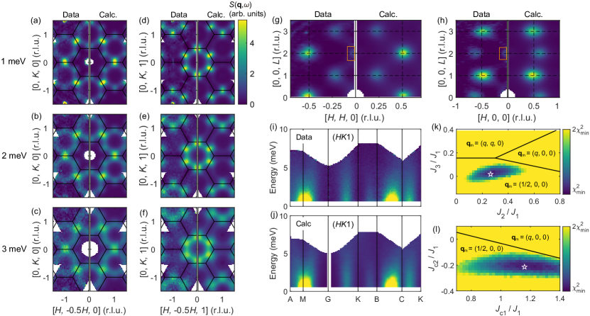
Figure 2: Least-squares fitting of the four-dimensional $S(\mathbf{q},\omega)$ maps from the paramagnetic phase of Co1/3TaS2 ($T>T_{\mathrm{N1}}$) using the LLD technique. (a)–(f) The left side of each panel shows the measured constant-$\omega$ cuts on the [$H$, $K$, 0] and [$H$, $K$, 1] planes with $\hbar\omega=1,2,$ and 3 meV. The right side shows the corresponding LLD simulation results from the optimal exchange parameter set suggested by our Bayesian optimization algorithm (Table 1). For better presentation, overall scaling factors of 2 and 3 are multiplied to $S(\mathbf{q},\omega)$ for $\hbar\omega=2,$ and 3 meV, respectively. (g)–(h) Similar cuts to (a)–(f) but on the [$H$, $H$, $L$] and [$H$, $0$, $L$] planes and at $\hbar\omega=1.5$ meV. Orange rectangular boxes in (g) and (h) denote the acoustic phonon signals, which were masked during the optimization process. All constant-$\omega$ cuts are based on data measured with $E_{i}=$ 8.3 meV and include energy and momentum integrations of $\pm 0.5$ meV and $\pm 0.08L$ (r.l.u.), respectively. (i)–(j) Measured and simulated energy-momentum slices along the high-symmetry lines in momentum space [see Fig. 1(e)]. Data from different $E_{i}$ values are overlaid. The masked low-energy region ($E<0.5\,$meV), dominated by quasi-elastic background signals, was not used for the fitting. (k)–(l) Goodness-of-fit (i.e., $\chi^{2}$-metric) maps around the optimal solution calculated by brute-force scans of the parameter space. White stars denote the best parameter set found by the Bayesian optimization algorithm, listed in Table 1 with uncertainty.

III.2 Analysis of paramagnetic excitation spectra

Rather than using the conventional method of spin-wave fitting in magnetically ordered states, we determined the exchange parameters $J_{n}$ and $J_{\mathrm{c}m}$ in Co1/3TaS2 by analyzing its energy-resolved paramagnetic excitation spectra through semi-classical LLD simulations. This approach offers the following two key advantages for studying Co1/3TaS2.

First, it does not rely on a predefined magnetic ground state, allowing for the determination of optimal exchange parameters independent of the magnetic structure. This flexibility enables a systematic comparison between experimental data and theoretical spin-wave spectra for both single-${\mathbf{Q}}$ and triple-${\mathbf{Q}}$ magnetic structures using a consistent set of exchange parameters. Such consistency is crucial for accurately identifying the correct ground state from spin-wave analysis. Notably, this approach was not employed in Ref. [25], which limited the ability of the previous work in discerning critical differences between the spin dynamics of single-${\mathbf{Q}}$ and triple-${\mathbf{Q}}$ magnetic structures below $T_{\mathrm{N}}$.

Second, analyzing the paramagnetic phase provides a more reliable estimate of the spin Hamiltonian, particularly when significant quantum effects beyond the LSWT are expected in the excitation spectrum below $T_{\mathrm{N}}$. These quantum effects, such as magnon decay, are generally pronounced in $S=1/2$ systems. Analyzing the paramagnetic phase using LLD has recently been recognized as a highly effective method for estimating the spin Hamiltonian in such cases [36, 35, 34]. Notably, as we discuss in Section III.D, the INS data of Co1/3TaS2 indicates the presence of nonlinear effects beyond LSWT in the triple-${\mathbf{Q}}$ phase.

The left panels of Figs. 2(a)-(h) and Fig. 2(i) display nine slices from a four-dimensional $S(\mathbf{q},\omega)$ map measured at 45 K ($T=1.18$$T_{\mathrm{N}1}$), covering all principal directions in the $\mathbf{q}-\omega$ space. Despite broadening due to large thermal fluctuations, each slice shows a distinct distribution of $S(\mathbf{q},\omega)$ along both the ${\mathbf{q}}$ and $\omega$ axes. For example, the strongest diffuse scattering signal at the M points of the Brillouin zones exhibits an elongated shape towards the [H, 0, 0] or its symmetry-equivalent directions in constant-$\omega$ cuts [e.g., Fig. 2(a) and 2(d)]. These patterns across the nine slices put sufficient constraints on estimating multiple bilinear exchange parameters with high accuracy (see Appendix D and Fig. 9). The exchange parameters of Co1/3TaS2 were refined through least-squares fitting of our LLD simulations to the nine measured $S(\mathbf{q},\omega)$ slices in Fig. 2. To efficiently search for a global minimum of the goodness-of-fit in a reasonable time frame, we adopted an advanced optimization algorithm, specifically Bayesian optimization, detailed in Appendix C.

The right panels of Figs. 2(a)-(h) and Fig. 2(j) show the LLD simulation results obtained using the best-fit parameter set ($J_{1},J_{2},J_{3},J_{c1},J_{c2}$) suggested by the Bayesian optimization algorithm. These results demonstrate remarkable agreement with the observed $S(\mathbf{q},\omega)$, indicating that these five exchange interactions effectively capture the spin Hamiltonian of Co1/3TaS2. The optimal parameter set and their uncertainties are summarized in Table 1. Notably, the nearest-neighbor interlayer exchange $J_{c1}$ is larger than the nearest-neighbor intralayer exchange $J_{1}$, reflecting the 3D nature of the spin Hamiltonian. The solution suggested by our optimization algorithm has been further validated by examining the $\chi^{2}$ metric — the measure of goodness-of-fit — around the optimal solution in the ($J_{1},J_{2},J_{3},J_{c1},J_{c2}$) parameter space [Figs. 2(k)–(l)]. A well-defined minimum of $\chi^{2}$ ($\chi^{2}_{\mathrm{min}}$) is indeed found at the position indicated by the optimization algorithm (white stars). Additional diagnostic analyses, as described in Appendix D, further corroborate the solution.

Table 1: Optimal parameter set for the five exchange interactions ($J$) and individual standard deviations ($\sigma_{J}$). We used $S=3/2$ for the spin length. The relative magnitudes to $J_{1}$ are also listed for easier comparison with theoretical magnetic phase diagrams in Fig. 2(k)–(l).

	$J_{1}$	$J_{2}$	$J_{3}$	$J_{c1}$	$J_{c2}$
$J$ (meV)	1.212	0.320	0.022	1.406	-0.260
$\sigma_{J}$ (meV)	$\pm$0.104	$\pm$0.061	$\pm$0.036	$\pm$0.097	$\pm$0.036
$J/J_{1}$	1	0.264	0.018	1.160	-0.215
Bond length (Å)	5.75	9.96	11.5	6.80	8.91

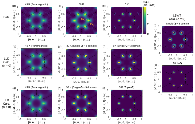
Figure 3: Distinct long-wavelength magnetic excitation spectra of the paramagnetic, stripe single-${\mathbf{Q}}$ and tetrahedral triple-${\mathbf{Q}}$ states. (a)–(c) Constant-$\omega$ slices at $\hbar\omega=1.2$ meV measured at (a) 45 K ($T_{\mathrm{N}1}$ $<T$), (b) 30 K ($T_{\mathrm{N2}}<T<T_{\mathrm{N1}}$), and (c) 5 K ($T<T_{\mathrm{N2}}$). $v_{\parallel}$ and $v_{\perp}$ in (b) denote $v_{1}(\mathbf{q}\,//\,\mathbf{Q}_{\nu})$ and $v_{1}(\mathbf{q}\perp\mathbf{Q}_{\nu})$, respectively; see Section III. A. (d)–(f) LLD simulation results corresponding to (a)–(c) obtained from the Hamiltonian determined above $T_{\mathrm{N}1}$, but without finite $K$. This results in single-${\mathbf{Q}}$ spin dynamics at both (e) 30 K and (f) 5 K. (g)–(i) Same as (d)–(f) but with finite $K>0$, resulting in single-${\mathbf{Q}}$ and triple-${\mathbf{Q}}$ spin dynamics at 30 and 5 K, respectively (see Fig. 10 in Appendix E). All constant-$\omega$ cuts are based on the data measured with $E_{i}=$ 5.8 meV and include energy and momentum integrations of $\pm 0.3$ meV and $\pm 0.08L$ (r.l.u.), respectively. (j)–(k) LSWT simulation results of the INS spectra in (b)–(c), which, unlike the LLD simulations, do not include any thermal fluctuation effects.

Overlaying the $\chi^{2}(J_{1},J_{2},J_{3},J_{c1},J_{c2})$ map on a theoretical magnetic phase diagram at $T=0$ elucidates the magnetic order suggested by our spin model. The phase boundaries, calculated from classical Monte-Carlo simulations, are shown on the $\chi^{2}$ map in Figs. 2(k)–(l). The optimal parameter set indeed stabilizes a magnetic order with $\mathbf{Q}_{\nu}$ = $\mathbf{G}_{\nu}/2$ or its symmetry-equivalent vectors [i.e., $\tilde{J}_{\mathbf{q}}$ has a global minimum at ${\mathbf{Q}}$ = $\mathbf{G}_{\nu}/2$], in accordance with observations in Co1/3TaS2 [Fig. 1(b)] [25, 26]. However, this does not reveal whether the ground state is triple-${\mathbf{Q}}$ or single-${\mathbf{Q}}$, as they are degenerate under isotropic bilinear exchange interactions. It should be noted that estimating $K$ from the high-temperature spectrum fitting is subject to substantial uncertainty due to its smaller magnitude relative to $|J_{1}|$. For instance, Figs. 3(d) and 3(g), which show constant-$\omega$ slices without and with finite $K$, are almost identical. Nevertheless, as we will demonstrate in the next section, successfully determining the bilinear interaction coefficients is sufficient to distinguish single-${\mathbf{Q}}$ and triple-${\mathbf{Q}}$ magnetic ground states from spin-wave spectra.

III.3 Long-wavelength magnon spectra

With the bilinear exchange interactions determined at $T>$ $T_{\mathrm{N}}$, we show that analyzing long-wavelength magnetic excitations in an ordered phase can effectively differentiate between a single-domain triple-${\mathbf{Q}}$ phase and a triple-domain single-${\mathbf{Q}}$ phase. As described in Section III. A, the acoustic magnon branches of Co1/3TaS2 around $\mathbf{Q}_{\nu}$ (${\mathbf{k}}=\mathbf{q}-\mathbf{Q}_{\nu}$ with $|{\mathbf{k}}|\ll 1$) consist of linear and quadratic modes for both the triple-${\mathbf{Q}}$ and single-${\mathbf{Q}}$ orderings. However, the anisotropy of the linear magnon mode [$\mathbf{v}_{\mathrm{L}}({\mathbf{k}})$] can be largely different depending on the specific magnetic structure.

The in-plane profile of $\mathbf{v}_{\mathrm{L}}(\mathbf{k})$ can be visualized by plotting a constant-$\omega$ slice of $S(\mathbf{q},\omega)$ with $\hbar\omega$ set sufficiently below the overall energy bandwidth of the magnetic excitations. For example, an isotropic $\mathbf{v}_{\mathrm{L}}({\mathbf{k}})$ will produce a circular pattern centered at $\mathbf{q}=\mathbf{Q}_{\nu}$ in the constant-$\omega$ slice, while a higher velocity along $\mathbf{k}\,//\,\mathbf{Q}_{\nu}$ ($v_{\parallel}>v_{\perp}$) will result in an ellipsoidal pattern elongated in the direction perpendicular to $\mathbf{Q}_{\nu}$. See the orange text and arrows in Fig. 3 (b) or Fig. 11 in Appendix F.

Figs. 3(a)-(c) show the constant-$\omega$ slices of $S(\mathbf{q},\omega)$ at $\hbar\omega=1.2$ meV, each measured from the paramagnetic (45 K, $T>T_{\mathrm{N1}}$), the intermediate (30  K, $T_{\mathrm{N2}}<T<T_{\mathrm{N1}}$), and the low-$T$ (5 K, $T<T_{\mathrm{N2}}$) phases, respectively. While, as shown in Fig. 3(b), the intermediate phase possesses strong in-plane anisotropy of $\mathbf{v}_{\mathrm{L}}({\mathbf{k}})$, the low-$T$ phase exhibits nearly isotropic $\mathbf{v}_{\mathrm{L}}({\mathbf{k}})$, as shown in Fig. 3(c). This contrast suggests a distinct nature of the magnetic structures in the temperature $T_{\mathrm{N2}}<T<T_{\mathrm{N1}}$ and $T<T_{\mathrm{N2}}$, despite both having the same $\mathbf{Q}_{\nu}$.

Comparing the observed spectra with the corresponding LLD simulation results with and without finite $K>0$ demonstrates that the intermediate and low-$T$ phases are single-${\mathbf{Q}}$ and triple-${\mathbf{Q}}$, respectively. It is important to note that for these simulations, we consistently use the optimal bilinear exchange parameter set determined at $T>T_{\mathrm{N1}}$. First, as shown in Fig. 10(b) of Appendix E, the triple-${\mathbf{Q}}$ ordering does not appear in the classical thermodynamic phase diagram for $K=0$, thereby yielding a single-${\mathbf{Q}}$ magnon spectrum at both 30 and 5 K, as shown in Figs. 3(e) and 3(f) respectively. Contrary to the experimental observations, the simulated spectra at 30 and 5 K display nearly the same $\mathbf{v}_{\mathrm{L}}({\mathbf{k}})$, except that the 30 K spectrum is broader due to enhanced thermal fluctuations. The calculation result remain similar for negative $K$, as the system still retains the stripe single-${\mathbf{Q}}$ ground state.

On the other hand, the simulation results with $K=0.06J_{1}$ successfully capture the measured spectra. LLD simulations of this model reproduce the two-step phase transition process depicted in Fig. 1(a) [see also Fig. 10(a) in Appendix E] and consequently provide triple-${\mathbf{Q}}$ magnon spectra at 5 K [Fig. 3(i)] and single-${\mathbf{Q}}$ spectra at 30 K [Fig. 3(h)]. Notably, such an intermediate phase stabilized by thermal disorder can only be simulated by techniques that incorporate thermal fluctuations, such as the LLD. The LLD simulations reproduce both the anisotropic $\mathbf{v}_{\mathrm{L}}({\mathbf{k}})$ observed at 30 K [Fig. 3(b)] and the isotropic $\mathbf{v}_{\mathrm{L}}({\mathbf{k}})$ at 5 K [Fig. 3(c)]. In other words, the combination of the optimal exchange parameter set determined at $T>T_{\mathrm{N1}}$ and $K>0$ describes the spin dynamics observed in all three phases simultaneously. This result not only supports the parameters presented in Table 1, but also provides evidence that the phases at $T<T_{\mathrm{N2}}$ and $T_{\mathrm{N2}}<T<T_{\mathrm{N1}}$ correspond to the triple-${\mathbf{Q}}$ and single-${\mathbf{Q}}$ orderings, respectively.

Another noticeable contrast between these two magnetic orderings is the intensity of quadratic magnon modes. This contrast is more clearly illustrated in Figs. 3(j)–(k), showing the single-${\mathbf{Q}}$ and triple-${\mathbf{Q}}$ magnon spectra calculated at 0 K using LSWT, which does not include thermal fluctuation effects. Although a quadratic mode signal is still present in both the single-${\mathbf{Q}}$ and triple-${\mathbf{Q}}$ calculations, its relative spectral weight compared to the linear mode is extremely weak in the triple-${\mathbf{Q}}$ phase. This observation is consistent with our data at 30 and 5 K, further supporting that $T_{\mathrm{N}2}$ marks to the transition between the tetrahedral triple-${\mathbf{Q}}$ and stripe single-${\mathbf{Q}}$ orderings.

We further investigate whether the observed anisotropic (nearly isotropic) $\mathbf{v}_{\mathrm{L}}({\mathbf{k}})$ is a characteristic dynamical property of the single-${\mathbf{Q}}$ (triple-${\mathbf{Q}}$) phase in a triangular lattice system. To confirm this, in Fig. 4, we analyze the degree of anisotropy in $\mathbf{v}_{\mathrm{L}}({\mathbf{k}})$ across a wide parameter space. This anisotropy can be quantified by the ratio $v_{\perp}/v_{\parallel}$, where $v_{\parallel}$ and $v_{\perp}$ are $\mathbf{v}_{\mathrm{L}}({\mathbf{k}})$ for $\mathbf{k}\parallel\mathbf{Q}_{\nu}$ and $\mathbf{k}\perp\mathbf{Q}_{\nu}$, respectively [see Section III. A and orange texts in Fig. 3(b)]. Figs. 4(a)–(b) show $v_{\perp}/v_{\parallel}$ for the triple-${\mathbf{Q}}$ and single-${\mathbf{Q}}$ orderings as a function of $J_{3}/J_{1}$ and $J_{2}/J_{1}$, using the optimal interlayer exchange parameters: $J_{c1}=1.16J_{1}$ and $J_{c2}=-0.22J_{1}$. Interestingly, $v_{\perp,t}/v_{\parallel,t}$ (anisotropy ratio for the triple-${\mathbf{Q}}$ phase) remains close to 1 across the wide parameter space, whereas $v_{\perp}/v_{\parallel}$ of the single-${\mathbf{Q}}$ phase ($v_{\perp,s}/v_{\parallel,s}$) generally deviates significantly from 1.

Furthermore, this contrast remains qualitatively intact even with reduced or zero interlayer interactions (i.e., 2D spin Hamiltonian). This is illustrated in Fig. 4(c)–(f), which display the $v_{\perp,t}/v_{\parallel,t}$ and $v_{\perp,s}/v_{\parallel,s}$ maps resulting from much weaker or zero $J_{c1}$ and $J_{c2}$. Thus, the distinction in $\mathbf{v}_{\mathrm{L}}({\mathbf{k}})$ between the single-${\mathbf{Q}}$ and triple-${\mathbf{Q}}$ phases persists across a broad range of exchange parameters. See Fig. 11 in Appendix F for a more explicit presentation of this contrast.

Figure 4: Distinct anisotropy in the linear magnon’s velocity [$v_{\mathrm{L}}(\mathbf{k})$] between the tetrahedral triple-${\mathbf{Q}}$ and stripe single-${\mathbf{Q}}$ magnetic structures. (a) $J_{2}/J_{1}$ and $J_{3}/J_{1}$ dependence of $v_{\perp}/v_{\parallel}$ for the triple-${\mathbf{Q}}$ phase calculated by LSWT, where $v_{\parallel}$ and $v_{\perp}$ are $v_{\mathrm{L}}(\mathbf{k}\,//\,\mathbf{Q}_{\nu})$ and $v_{\mathrm{L}}(\mathbf{k}\perp\mathbf{Q}_{\nu})$, respectively; see Fig. 3(b). (b) Same as (a), but for the single-${\mathbf{Q}}$ phase. For the calculations in (a) and (b), the optimal values of $J_{\mathrm{c1}}$ and $J_{\mathrm{c2}}$ were used (Table 1). (c)–(f) Same as (a)-(b), but calculated with (c)–(d) reduced and (e)–(f) zero interlayer interactions $J_{\mathrm{c1}}$ and $J_{\mathrm{c2}}$. Empty regions in the color plots indicate instability of the stripe single-${\mathbf{Q}}$ or tetrahedral triple-${\mathbf{Q}}$ magnetic orderings for given $J_{2}/J_{1}$ and $J_{3}/J_{1}$. (g)–(h) Illustrations of tetrahedral triple-${\mathbf{Q}}$ and stripe single-${\mathbf{Q}}$ orderings, providing an intuitive understanding on their inherently isotropic and anisotropic Fourier-transformed interaction matrix $J(\mathbf{q})$, respectively.

The nearly isotropic $v_{\perp,t}/v_{\parallel,t}$ and strongly anisotropic $v_{\perp,s}/v_{\parallel,s}$ can also be understood from our analytic theory calculations in Section III. A. Specifically, $v_{\perp,s}/v_{\parallel,s}$ can vary from 0 to infinity (i.e., no upper or lower bound), whereas $v_{\perp,t}/v_{\parallel,t}$ is strictly limited from $\sqrt{1/3}=0.58$ to $\sqrt{3}=1.732$. Furthermore, the variation of $v_{\perp,t}/v_{\parallel,t}$ within the parameter space is not uniform; it changes rapidly around the phase boundary of $\mathbf{Q}_{\nu}$ = $1/2\mathbf{G}_{\nu}$ and converges toward its upper or lower bound at the boundary. As a result, the expected deviation of $v_{\perp,t}/v_{\parallel,t}$ from 1 across the entire parameter space is much smaller than what is implied by the upper ($\sqrt{3}$) and lower ($\sqrt{1/3}$) bounds. Indeed, average and standard deviation values of the $v_{\perp,t}/v_{\parallel,t}$ map in Fig. 4(a) and 4(e) are $1.07\pm 0.02$ and $1.00\pm 0.04$, demonstrating its narrow distribution centered around 1. On the other hand, the variation of $v_{\perp,s}/v_{\parallel,s}$ in the parameter space is much more pronounced, meaning that $v_{\perp,s}/v_{\parallel,s}\sim 1$ is realized only in a very confined region of the parameter space. These observations consistently suggest the robust capability of $\mathbf{v}_{\mathrm{L}}({\mathbf{k}})$ in distinguishing between single-${\mathbf{Q}}$ and triple-${\mathbf{Q}}$ orderings, which would be even valid for the 2D spin Hamiltonian (i.e. 2D magnets). We also note that $K$ has little impact on these results mainly due to its order-of-magnitude smaller size than the bilinear exchange parameters, which is typically the case in real materials (see Appendix F). The only role of $K$ is to select the triple-${\mathbf{Q}}$ ordering and consequently gap out the quadratic mode associated with the aforementioned accidental degeneracy.

An intuitive understanding of the nearly isotropic (strongly anisotropic) $\mathbf{v}_{\mathrm{L}}({\mathbf{k}})$ in the triple-${\mathbf{Q}}$ (single-${\mathbf{Q}}$) phase can be gained from its real-space spin configuration [Fig. 4(g)–(h)]. The tetrahedral triple-${\mathbf{Q}}$ ground state preserves the three-fold rotation symmetry about the $c$-axis, i.e., the six exchange paths of $J_{n}$ ($n$ is integer) always connect two spins with the same relative angle $\theta=\mathrm{cos}^{-1}(-1/3)$. This information enters $\tilde{J}_{\mathbf{q}}^{aa}$–a quantity directly related to magnon velocity (see section III. A)–as a momentum-independent phase factor. However, the stripe single-${\mathbf{Q}}$ ground state breaks the three-fold symmetry, meaning that two exchange paths perpendicular to $\mathbf{Q}_{\nu}$ connect ferromagnetically aligned spins, while the other four paths connect antiferromagnetically aligned spins. This difference appears in $\tilde{J}_{\mathbf{q}}^{aa}$ as reversed phase factors for ${\mathbf{q}}$$\,//\,$$\mathbf{Q}_{\nu}$ and ${\mathbf{q}}$$\,\perp\,$$\mathbf{Q}_{\nu}$, naturally introducing anisotropy between $v_{\parallel}$ and $v_{\perp}$.

Notably, the context above suggests that the distinct $\mathbf{v}_{\mathrm{L}}({\mathbf{k}})$ characteristics between the single-${\mathbf{Q}}$ and triple-${\mathbf{Q}}$ ground states may qualitatively persist even in the case of incommensurate ordering wave vectors ($\mathbf{Q}_{\nu}$ $=(q,0,0)$ with $0<q<1/2$). Regardless of its modulation period, a single-${\mathbf{Q}}$ spiral phase always has a ferromagnetic spin alignment along the bond vectors ($\mathbf{\delta}$) perpendicular to $\mathbf{Q}_{\nu}$, whereas three-fold symmetry ($C_{3z}$) of the triple-${\mathbf{Q}}$ structure guarantees a uniform relative spin angle for all six bonds of $J_{n}$. This implies that $\mathbf{v}_{\mathrm{L}}({\mathbf{k}})$ could serve as an effective diagnostic tool for a general single-${\mathbf{Q}}$ versus triple-${\mathbf{Q}}$ problem on a triangular lattice.

Figure 5: Full magnon spectra of the stripe single-${\mathbf{Q}}$ and tetrahedral triple-${\mathbf{Q}}$ magnetic orderings. (a)–(b) Magnetic spectrum measured at 30 K along the high-symmetry lines on the [$H$, $K$, 1] and [$H$, $K$, 2] planes [see Fig. 1(e)]. (c)–(d) Same as (a)–(b), but measured at 5 K. The energy range not shown in these plots is dominated by quasi-elastic background signals. (e)–(h) LLD simulation results corresponding to (a)–(d), respectively. Note that the colorplots in this figure shows dynamical susceptibility ($\chi^{\prime\prime}(\mathbf{q},\omega)$). Orange arrows in (c)–(d) and (g)–(h) indicate apparent discrepancies between the data and simulation results for the triple-${\mathbf{Q}}$ phase, suggesting the presence of additional effects beyond the non-interacting magnon picture.

Figure 6: Magnon energy renormalization in the tetrahedral triple-${\mathbf{Q}}$ phase. (a)–(b) Comparison between the INS data and LLD simulation results at 30 K through constant-$\omega$ (4 meV) and ${\mathbf{Q}}$ ($\mathbf{q}_{\alpha}$) cuts from Figs. 5(a) and 5(e). The dashed brown line in (b) represents the estimated quasielastic background signal based on a single Gaussian peak fitting. (c)–(d) Same as (a)–(b), but for 5 K [Figs. 5(c) and 5(g)]. (e) Momentum positions $\{\mathbf{q}_{h}\}$ (dashed orange lines) where sizable magnon energy renormalization is observed at 5 K. Red-, orange-, and yellow-filled circles indicate $\mathbf{q}_{\alpha}$, $\mathbf{q}_{\beta}$, and $\mathbf{q}_{\gamma}$ in (c), respectively. The three solid arrows illustrate a decay process of a single magnon on $\{\mathbf{q}_{h}\}$ (red) into two magnons. (f) Diagrammatic representation of the magnon decay process depicted in (e). $\mathbf{Q}_{\nu}$ denotes three ordering wave vectors ($\nu=1,2,3$) corresponding to the three M points of the Brillouin zone. (g) A constant-$\omega$ slice at 3.5 meV on the [$H$, $K$, 1] plane, demonstrating the magnon signal along the line $\{\mathbf{q}_{h}\}$. (h) Non-interacting two-magnon density of states (DOS) calculated from bare one-magnon dispersion. Black solid lines show the one-magnon dispersion obtained from LSWT.

III.4 Failure of non-interacting magnon picture in the triple-${\mathbf{Q}}$ phase

In addition to our comprehensive analysis of long-wavelength magnetic excitations, the full spin-wave spectrum of Co1/3TaS2 provides more insights into the nature of the triple-${\mathbf{Q}}$ and single-${\mathbf{Q}}$ spin dynamics. Figs. 5(a)–(b) and 5(c)–(d) show the magnon spectra over a wide energy-momentum space at 5 K (single-${\mathbf{Q}}$) and 30 K (triple-${\mathbf{Q}}$), respectively. The most conspicuous feature of these spectra is their broadness. For the 5 K spectra, where thermal fluctuations are minimal, this broadness is undoubtedly an intrinsic feature rather than an artifact of sample mosaicity or instrumental resolution effects. This is evidenced by the fact that the phonon branches observed in the high-${\mathbf{Q}}$ region of the same dataset exhibit much sharper spectra (see Fig. 13 in Appendix H). This observation, at least for the triple-${\mathbf{Q}}$ phase, indicates a clear breakdown of the non-interacting magnon picture. On the other hand, sizable thermal fluctuations contribute significantly to the broadness for the single-${\mathbf{Q}}$ spectra measured at 30 K, (= 0.79$T_{\mathrm{N}1}$), which is difficult to disentangle from the intrinsic linewidth broadening relevant to finite magnon lifetime. Thus, although some intrinsic broadening likely exists at 30 K as well, it is less clear than at 5 K.

Figs. 5(e)–(h) show the magnon spectra simulated by LLD using the parameters in Table 1 and $K=0.06J_{1}$. For $\hbar\omega>10\,$meV, where the optical branches appear in our LLD simulation [Figs. 5(f) and 5(h)], the INS spectra are heavily damped for both the single-${\mathbf{Q}}$ and triple-${\mathbf{Q}}$ phases compared to the simulation results. While this makes a more detailed comparison with the LLD simulations challenging, such deviations from the spin-wave theory’s predictions, which are based on a fully localized picture of the magnetic moments, are commonly observed for high-energy excitations in metallic antiferromagnets [49, 50, 51, 52, 53]. This phenomenon is associated with the prevalence of the Stoner continuum in their energy-momentum space, whose influence generally increases with energy transfer [49, 50, 51, 54]. This metallic character may also be responsible for the reduced ordered moment of Co1/3TaS2 in the triple-${\mathbf{Q}}$ phase: $\mu_{s}=1.3\mu_{\mathrm{B}}$ [25], which is less than half of the value expected for a fully localized scenario ($gS=3\mu_{\mathrm{B}}$) [55].

Nevertheless, further analysis of the low-energy region ($\hbar\omega<10$ meV) suggests that the Stoner continuum may not fully explain the spin dynamics beyond LSWT in Co1/3TaS2. A clear magnon dispersion observed in this low-energy region still offers insights when comparing the data with the results of LLD simulations. At 30 K, LLD shows overall satisfactory agreement with the data regarding magnon dispersion [Figs. 5(a)–(b) and 5(e)–(f)], which is further demonstrated by the constant-${\mathbf{Q}}$ and constant-$\omega$ cuts in 6(a)–(b). While LLD overestimates the intensity at low energy transfer values around the M point [see Fig. 5(a) and 5(e)], this is partially attributed to a calculation artifact: the gapless linear mode at the M point possesses a diverging structure factor in the calculation, which, due to resolution convolution, generates sizable intensity that extends up to finite energy transfer values in the simulation.

Despite exhibiting a similar magnon spectrum to that of the single-${\mathbf{Q}}$ phase, the spectrum of the triple-${\mathbf{Q}}$ phase measured at 5 K shows an apparent inconsistency with the magnon dispersion obtained from LLD simulations. The orange arrows indicate this discrepancy in Figs. 5(c)–(d) and 5(g)–(h): although our calculation reproduces a local minimum of the magnon dispersion at these ${\mathbf{Q}}$ points, it predicts a much shallower dip into lower energy [see also Fig. 6(c)–(d)]. Importantly, such steep downward dispersion cannot be reproduced by any reasonable set of exchange parameters in LLD; see Appendix H and Fig. 14 therein. We note that the LLD simulation result is nearly identical to that of LSWT at this temperature, suggesting the presence of substantial magnon energy renormalization beyond LSWT in the triple-${\mathbf{Q}}$ phase. This contrasts with he single-${\mathbf{Q}}$ phase at 30 K, where the LLD calculation, incorporating thermal fluctuations, largely captures the deep downward dispersion. Note that the deep downward dispersion observed at 30 K is attributed to both a steeper magnon dispersion in the single-$\mathbf{Q}$ phase and the sizable thermal fluctuations at 30 K, further depressing the dispersion minimum in the spectrum.

Our findings from this comparative analysis–the magnon energy renormalization is more pronounced in the triple-${\mathbf{Q}}$ phase–hints at its microscopic origin. In Co1/3TaS2, potential origins for this renormalization include: (i) interactions between magnons and conduction electrons (i.e., renormalization by the Stoner continuum), and (ii) magnon-magnon interactions (i.e., renormalization by the multi-magnon continuum). However, these two factors depend differently on the detailed spin configuration. The second mechanism is significantly enhanced when a magnetic structure becomes noncollinear due to the generation of cubic vertices [56, 57, 58]. This leads to significantly larger magnon decay and renormalization in the noncollinear triple-${\mathbf{Q}}$ ordering compared to the collinear single-${\mathbf{Q}}$ ordering. On the other hand, the effect of the Stoner continuum is anticipated to be similar in both magnetic structures or even smaller in a noncollinear magnet since a Stoner excitation process requires a full spin flip. See Appendix I for further explanation. Thus, our observation agrees better with the magnon-magnon interaction mechanism, suggesting that it is the primary origin of energy renormalization.

Interestingly, the ${\mathbf{q}}$ positions where pronounced energy renormalization occurs provide unique insights into the three-magnon process of the tetrahedral triple-${\mathbf{Q}}$ ordering. These ${\mathbf{q}}$ positions, $\mathbf{q}_{\alpha,\beta,\gamma}$ in Figs. 5(c) and 6(c)–(d), lie on the hexagon that connects the six M points of a Brillouin zone [denoted as $\{\mathbf{q}_{h}\}$ in Fig. 6(e)]. The intuition behind why this specific ${\mathbf{q}}$-path might be significant for the three-magnon process of the triple-$\mathbf{Q}$ phase relates to its stabilization mechanism, which involves Fermi surface nesting (or quasi-nesting). The M–ordering wave vectors extensively connect different positions on $\{\mathbf{q}_{h}\}$, thereby acting as nesting wave vectors when $\{\mathbf{q}_{h}\}$ corresponds to the Fermi surface and thus stabilizing the tetrahedral triple-${\mathbf{Q}}$ ordering [30, 59]. An analogous scattering process can occur for magnons: a magnon with $\mathbf{q}_{1}\in\{\mathbf{q}_{h}\}$ can decay into two magnons with $\mathbf{q}_{2}=\mathbf{Q}_{\nu}$ and $\mathbf{q}_{3}\in\{\mathbf{q}_{h}\}$, where $\mathbf{q}_{3}$ is equivalent to $\mathbf{q}_{1}$. An example of such a process is illustrated in Fig. 6(e)–(f). Importantly, the kinematic conditions for these three-magnon processes can always be satisfied since Goldstone modes arising from Eq. 1 has zero energy at $\mathbf{q}=\mathbf{Q}_{\nu}$. This implies observing the pronounced magnon-magnon interaction effects specifically at $\mathbf{q}\in\{\mathbf{q}_{h}\}$ is feasible. Indeed, a signal from the renormalized magnon mode is observed consistently across all positions on $\{\mathbf{q}_{h}\}$ [Fig. 6(g)].

For a deeper understanding, we calculated the energy and momentum-dependent two-magnon density-of-states (DOS), $D(\mathbf{q},\omega_{\mathbf{q}})$. Although accurate magnon energy renormalization can only be determined through non-linear spin-wave theory (NLSWT) [57, 60], applying NLSWT to the triple-$\mathbf{Q}$ ordering in Co1/3TaS2 is quite cumbersome due to its multiple magnetic sublattices. Instead, $D(\mathbf{q},\omega_{\mathbf{q}})$ can serve as a simple yet effective quantity to qualitatively examine the extent of the three-magnon process [54, 61, 34]. $D(\mathbf{q},\omega_{\mathbf{q}})$ is calculated by counting the number of three-magnon channels at $(\mathbf{q},\omega_{\mathbf{q}})$ that satisfy the kinematic condition:

$$D(\mathbf{q},\omega_{\mathbf{q}})=\,\frac{1}{N}\sum_{i,j}{\sum_{\mathbf{k}}{\delta(\omega_{\mathbf{q}}-(\omega_{\mathbf{k}}+\omega_{\mathbf{q-k}}))}},$$ (17)

where $N$ is a normalization factor, $\mathbf{k}$ runs over the set of $\mathbf{q}$ points in the first Brillouin zone, and $i$ and $j$ are the magnon band indices. Fig. 6(h) shows the calculated $D(\mathbf{q},\omega_{\mathbf{q}})$ on the $\Gamma-K-B$ lines, which encompasses $\mathbf{q}_{\alpha}$ and $\mathbf{q}_{\beta}$. Indeed, all magnon branches at around $\mathbf{q}_{\alpha}$ and $\mathbf{q}_{\beta}$ are embedded in the two-magnon continuum with sizable $D(\mathbf{q},\omega_{\mathbf{q}})$, supporting our interpretation of magnon decay and renormalization due to magnon-magnon interactions. Nonetheless, a more detailed analysis based on NLSWT is necessary to rigorously confirm our scenario, and we leave this as a future theoretical challenge.

IV Summary and Discussion

Using Co1/3TaS2, which exhibits both the single-$\mathbf{Q}$ and triple-$\mathbf{Q}$ magnetic ground states at different temperatures, we have successfully highlighted the distinct characteristic dynamical properties of these phases on a triangular lattice. Our comprehensive analysis suggests that measuring long-wavelength (= low-energy) magnetic excitation spectra in both the paramagnetic and ordered phases can significantly aid in identifying the nature of long-range order. A crucial step in this process was obtaining an unbiased optimal exchange parameter set from the paramagnetic phase using the high-temperature simulation techniques based on LLD [33]. We note that this approach remains accurate even in quantum spin systems $S=1/2$, as demonstrated in recent studies [36, 34, 35]. To better convey our findings, we summarize our distinction protocol below:

1. Measure the magnetic excitation spectra of the paramagnetic phase ($T>T_{\mathrm{N}}$) and refine the spin Hamiltonian by fitting these spectra.

2. Measure long-wavelength excitation spectra of the ordered phase of interest ($T<T_{\mathrm{N}}$) and compare the results with the theoretical spectra of the single-${\mathbf{Q}}$ and triple-${\mathbf{Q}}$ phases. The theoretical calculations should use the spin Hamiltonian refined from the paramagnetic excitation spectra, which will likely yield different profiles of Goldstone mode dispersion for the triple-$\mathbf{Q}$ and single-$\mathbf{Q}$ orderings.

Identifying a triple-${\mathbf{Q}}$ ground state through long-wavelength excitations has significant merits from both theoretical and experimental perspectives. Theoretically, the long-wavelength approximation simplifies the profile of magnon dispersion into a universal scheme governed by the Goldstone theorem. This not only enables simple analytic calculations of the magnon dispersion but also ensures robustness against additional effects that could complicate the picture. For instance, magnons in metallic systems usually experience substantial decay or renormalization, especially in higher energies, due to interactions with conduction electrons. Moreover, in systems with highly itinerant magnetism, the Heisenberg model itself might not be a valid Hamiltonian for describing their magnetic dynamics [55]. Nevertheless, the Goldstone theorem indicates the presence of well-defined collective excitations in the long-wavelength limit (linear modes in Eq. 10), ensuring that our analysis based on Eq. 1 and LSWT remains valid even in such situations. This also applies to systems influenced by significant quantum fluctuations (e.g., $S=1/2$ systems); while the non-interacting magnon picture may fail across a wide energy-momentum space, it still holds in the long-wavelength limit. Experimentally, long-wavelength excitations around ${\mathbf{q}}$=$\mathbf{Q}_{\nu}$ typically exhibit the strongest dynamical structure factor in a magnetic excitation spectrum, allowing for high-quality measurements even in systems with weak magnetic signals. These considerations suggest that identifying the single-$\mathbf{Q}$ and triple-${\mathbf{Q}}$ phases based on $\mathbf{v}_{\mathrm{L}}({\mathbf{k}})$ may be applicable to a broad range of magnetic materials, regardless of their specific characteristics.

There are a few intriguing materials that warrant the application of this approach. First, Co1/3NbS2, a metallic antiferromagnet isostructural to Co1/3TaS2, also exhibits magnetic Bragg peaks at $\mathbf{Q}_{\nu}=\mathbf{G}_{\nu}/2$ or its symmetry-related positions [62] and a sizable $\sigma_{xy}(\mathbf{H}=0)$ [63]. Notably, however, it possesses an additional incommensurate ordering wave vector perpendicular to $\mathbf{Q}_{\nu}=\mathbf{G}_{\nu}/2$ [64], which compromises the symmetry argument associated with the $\tau_{1a}T$ operation used in Co1/3TaS2 to confirm the triple-${\mathbf{Q}}$ ground state. For the spin configuration of $\mathbf{Q}_{\nu}=\mathbf{G}_{\nu}/2$, both tetrahedral triple-${\mathbf{Q}}$ and stripe single-${\mathbf{Q}}$ orderings have been suggested as candidate ground states [26, 64, 62, 65]. Although the origin of the co-existing commensurate and incommensurate modulations is unclear, measuring its long-wave excitation spectra will tell which ground state is correct for $\mathbf{Q}_{\nu}=\mathbf{G}_{\nu}/2$.

Another promising candidate for the application is Na2Co2TeO6, which has recently garnered significant interest as a candidate material for the Kitaev honeycomb model with a putative proximate spin-liquid phase [66, 67, 68]. Notably, Na2Co2TeO6 shares the same space group and $\mathbf{Q}_{\nu}$ as Co1/3TaS2. In this compound, both collinear single-${\mathbf{Q}}$ [69, 70, 71] and non-coplanar triple-${\mathbf{Q}}$ [72, 73, 74] magnetic structures have been suggested as potential ground states. While the latter scenario has been supported convincingly, applying the approach introduced in this work could help undoubtedly confirm the true magnetic ground state of this intriguing compound. In addition, successful application to Na2Co2TeO6 could be a meaningful milestone in extending this approach to a more 2D magnetism: unlike Co1/3TaS2, Na2Co2TeO6 has negligible interlayer interactions and can be considered a 2D hexagonal antiferromagnet [72]. While our analysis of $\mathbf{v}_{\mathrm{L}}({\mathbf{k}})$ already implies the feasibility of our approach even in the case of negligible inter-layer interactions, an experimental demonstration would further promote the investigation of triple-${\mathbf{Q}}$ spin textures in 2D systems.

In the context of 2D magnetism above, an intriguing question arises: would the triple-$\mathbf{Q}$ structure demonstrated in this study persist in atomically-thin Co1/3TaS2? Notably, recent studies on the isostructural family TM1/3TaS2 [28, 29] suggest the capability of producing a few nm-thick or even monolayer Co1/3TaS2 via chemical intercalation (Co1/3TaS2 refers to Co-intercalated 2H-TaS₂). The bilinear exchange parameters determined in this work (Table 1) offer important insights into this question: even assuming zero interlayer interactions, $J_{cm}$, the in-plane exchange parameter set $J_{n}$ remain within the region of $\mathbf{Q}_{\nu}=\mathbf{G}/2$ [see Fig. 4]. Also, the source of the four-spin interaction $K$–the coupling between Co²⁺ localized moments and 5$d$ conduction electrons of Ta [25]– would remain present in the 2D limit. Thus, we speculate that the tetrahedral triple-$\mathbf{Q}$ state could persist in atomically-thin or monolayer Co1/3TaS2, even without the interlayer couplings. This possibility urges the exploration of reduced material thickness as a promising direction for future research on Co1/3TaS2.

The suggested significance of magnon-magnon interactions in Co1/3TaS2 also warrants more discussion. While magnon-magnon interaction is the most plausible explanation, to our best knowledge, for the enhanced renormalization in the triple-$\mathbf{Q}$ phase, it is rather unusual to observe such significant influence in a classical spin system ($S>1/2$). Previous studies consistently suggested that Co²⁺ ions in Co1/3TaS2 develop localized magnetic moments of $S=3/2$ via a high-spin $d^{7}$ configuration [75, 76, 62, 27, 25, 26]. In a triangular lattice antiferromagnet that develops coplanar 120^∘ ordering, quantum effects beyond LSWT are expected to be marginal for $S=3/2$ [60]. One possibility is that the non-coplanar triple-${\mathbf{Q}}$ phase exhibits much stronger magnon-magnon interactions than those in the 120^∘ phase. To confirm this, the analytic $1/S$ expansion calculation for the tetrahedral triple-${\mathbf{Q}}$ magnetic structure should be conducted, which, to our best knowledge, has not yet been done.

Even though it does not align well with our observation of temperature-dependent renormalization at $\{\mathbf{q}_{h}\}$, the Stoner continuum should not be excluded from a source of magnon decay and renormalization in the overall low-energy spectra ($<10$ meV) of Co1/3TaS2. While the two-magnon continuum can dominate over that of the Stoner continuum at specific momentum positions in a non-collinear magnet [54], the Stoner continuum would still play a role in the observed spectrum to some extent, considering that broad magnetic spectra are consistently observed in any metallic antiferromagnets [55, 49, 50, 51, 52, 77]. Possible Stoner excitation processes at $\mathbf{q}\in\{\mathbf{q}_{h}\}$ are qualitatively discussed in Appendix I. Generally, disentangling these two factors in an INS spectrum is very challenging and thus requires a specific situation where these two contributions behave differently [54]. We note that the contrasting magnitude of the magnon-magnon interactions between triple-${\mathbf{Q}}$ and single-${\mathbf{Q}}$ orderings–the key feature that led us to interpret our observation as being due to the two-magnon continuum rather than the Stoner continuum–applies only when $\mathbf{Q}_{\nu}$ = (1/2, 0, 0). For $\mathbf{Q}_{\nu}$ = ($q$, 0, 0) with $0<q<1/2$, the single-${\mathbf{Q}}$ phase is also non-collinear and can manifest nonzero three-magnon terms (except in the case of spin density wave).

We finally acknowledge one limitation of the spin Hamiltonian suggested in this work (Eq. 1): omission of magnetic anisotropy. Although the isotropic spin model in Eq. 1 captures the phase diagram and key spin dynamics we observed, the presence of a few small anisotropy terms is implied in its static and dynamic magnetic properties. First, as reported in Ref. [25], the triple-${\mathbf{Q}}$ phase develops a magnon energy gap (approximately 0.5 meV or smaller) at the M points. Interestingly, any symmetry-allowed single-ion anisotropy terms in Co1/3TaS2 cannot open this energy gap, indicating the presence of slight exchange anisotropy. Bond-dependent exchange anisotropy $J_{\pm\pm}$ is a rare term that can open this gap in the tetrahedral triple-$\mathbf{Q}$ phase; see Ref. [78] for its definition. Another component is the easy-axis anisotropy along the $c$-axis, which is necessary to describe the out-of-plane spin configuration of the single-${\mathbf{Q}}$ phase at $T_{\mathrm{N2}}<T<T_{\mathrm{N1}}$. This can be included in Eq. 1 as either the $XXZ$-type exchange anisotropy or single-ion anisotropy [$\hat{H}_{i}=K_{z}(\mathbf{S}^{z}_{i})^{2}$ where $K<0$ and $i$ indices triangular sites].

However, we emphasize that the observation of the tetrahedral triple-${\mathbf{Q}}$ ground state limits the size of these anisotropy terms to be smaller than $K$, as they would incur energy costs to its spatially uniform tetrahedral configuration. The observed energy gap of 0.5 meV at 5 K and the absence of any energy gap at 30 K (down to the precision of $0.3$ meV) further support their small magnitude. As the four-spin interaction term with the coefficient $K$ is shown to have marginal effects on the observed spin dynamics (Appendix F), these anisotropy terms with smaller coefficients than $K$ are unlikely to affect the spin dynamics analysis presented in this study.

Appendix A Co-aligned single crystals

Fig. 7 shows photos of the co-aligned Co1/3TaS2 single crystals used in this study. Their good alignment is evident in the diffraction spectra presented in Fig. 1(b).

Figure 7: The co-aligned Co1/3TaS2 single crystals used for the INS experiment. More details can be found in the Methods section of the main text.

Appendix B Higher-order renormalization of scalar bi-quadratic interactions

If a Hamiltonian term involves a nonlinear order of spin operators at a single site (i.e., higher than the first order), its amplitude becomes renormalized in higher-order spin wave theory [45]. The scalar biquadratic term used in Eq. 1 falls into this category. Based on the 1/$S$ expansion, the renormalized magnitude of $K$ ($\tilde{K}$) is derived as follows [45]:

$$\tilde{K}=(1-\frac{1}{S}+\frac{1}{4S^{2}})K$$ (18)

In other words, in Co1/3TaS2 ($S=3/2$), the actual magnitude of biquadratic interactions in the simulation ($=\tilde{K}$) is 4/9 of the input value ($K$). Since $\tilde{K}\sim 0.027J_{1}$ is needed to reproduce $T_{\mathrm{N}2}$/$T_{\mathrm{N}1}$ = 0.7, the input value of $K$ should be $\sim 0.06J_{1}$.

Appendix C Procedure of fitting paramagnetic excitation spectra

In this section, we describe the optimization process used to fit the paramagnetic excitation spectra using LLD. The optimal solution was found by performing the least-squares fitting between the nine measured and simulated $S(\mathbf{q},\omega)$ slices in Fig. 2. Completing this optimization job within a reasonable time frame requires a good understanding of its characteristics. A LLD simulation to calculate spin dynamics at finite temperatures is a forward simulation. Since this is fairly time-consuming (a few minutes for each slice of $S(\mathbf{q},\omega)$ in Fig. 2), it is crucial to minimize the number of times the optimization process runs this simulation. For this reason, using common gradient-based optimization methods, which require repeated evaluations of the simulation to calculate gradients, would be computationally expensive. This is especially true for our problem, as it deals with a high-dimensional space of variables due to multiple exchange interactions for both intralayer and interlayer bonds, and should fit a four-dimensional profile of $S(\mathbf{q},\omega)$. Moreover, forward simulations contain noise in their results, which further compromises the accuracy of gradient calculations.

To address this challenge, we adopted a Bayesian optimization algorithm, which is gradient-free and very effective for problems where the fitting object is difficult to evaluate due to computational costs. This approach reaches an optimal solution with relatively fewer iterations by performing intelligent parameter space searches based on the surrogate modeling and the acquisition function [79]. We used the Bayesian optimization package implemented in Python [80], with the Gaussian process for the surrogate model [81, 80]. The optimization algorithm searched a wide 5D parameter space of $J_{1}$, $J_{2}/J_{1}$, $J_{3}/J_{1}$, $J_{\mathrm{c1}}/J_{1}$, and $J_{\mathrm{c2}}/J_{1}$, with each parameter allowed to range as follows: $0.8\,\mathrm{meV}<J_{1}<1.4\,\mathrm{meV}$, $0<J_{2}/J_{1}<0.8$, $-0.15<J_{3}/J_{1}<0.4$, $0.7<J_{\mathrm{c1}}/J_{1}<1.4$, and $-0.4<J_{\mathrm{c2}}/J_{1}<0.1$.

The algorithm converged on the optimal parameter set shown in Table 1, or an equivalent set within the uncertainty range, after 150–200 Bayesian optimization steps. To ensure the credibility of the suggested solution, optimization was performed starting from several different initial parameter sets, and all trials reached the same solution. Additionally, to check if other non-trivial solutions exist or if the suggested solution is merely a local minimum of $\chi^{2}$, we conducted a brute-force exploration of the $\chi^{2}$ map around the optimal parameter set, as shown in Figs. 2(k)–(l). As mentioned in the main text, a unique minimum of $\chi^{2}$ ($\chi^{2}_{\mathrm{min}}$) was found at the solution’s position suggested by the optimization algorithm. Further assessment of this optimal solution is described in Appendix D.

Appendix D Reliability of the optimal parameter set found by Bayesian optimization

In addition to the nice agreement between the data and the simulations as shown in Figs. 2(a)–(j) and the well-identified $\chi^{2}$ minimum in Figs. 2(k)–(l), we further assess the reliability of the bilinear exchange parameters suggested by our Bayesian optimization algorithm.

First, the magnitudes of the interlayer exchange parameters $J_{c1}$ and $J_{c2}$ in Table 1 can be validated by examining the magnon spectrum along the [0, 0, $L$] direction, which exhibits simple V-shaped magnon branches [Figs. 8(a)–(b)]. In Figs. 8(a)–(b), we overlay the LSWT magnon dispersion calculated with the optimal exchange parameters and the triple-${\mathbf{Q}}$ magnetic ordering on the data. Also, the corresponding $S(\mathbf{q},\omega)$ maps calculated by LSWT, convoluted with instrumental resolution and momentum integration effects, are plotted in Figs. 8(c)–(d). Indeed, the optimal $J_{c1}$ and $J_{c2}$ parameters in Table 1 accurately capture the measured bandwidth along the [0, 0, $L$] direction.

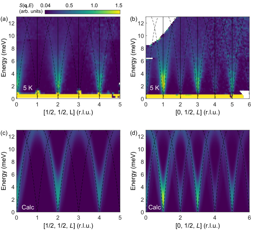
Figure 8: (a)–(b) Measured and (c)–(d) simulated magnon spectra along the [0, 0, $L$] direction at 5 K (i.e., the triple-${\mathbf{Q}}$ phase). The data collected from different $E_{i}$ are overlaid. Dashed black lines are the dispersion of linear magnon modes. The calculation results in this figure was obtained using LSWT.

Furthermore, we directly compared the paramagnetic excitation spectra of the optimal parameter set with those of surrounding parameter sets to evaluate the degradation in fit quality for these alternative solutions. Fig. 9 in Appendix D shows constant-$\omega$ slices of $S(\mathbf{q},\omega)$ simulated from the optimal parameter set [panel (c)] and from suboptimal sets [panels (d)–(e)] near the optimal solution. The $\chi^{2}$ metric of the chosen suboptimal solutions (white triangular and square symbols) is 1.25$\chi^{2}_{min}$, which is not far from $\chi^{2}_{\mathrm{min}}$. However, their $S(\mathbf{q},\omega)$ spectra exhibit clear discrepancies with the data; the signal’s pattern around the M point is more elongated to the [$H$, 0, 0] direction than observed while being narrower along the [$-0.5K$, $K$, 0] direction. Fig. 9(f) demonstrates this more explicitly. This comparison further confirms the reliability of the fitted exchange parameters.

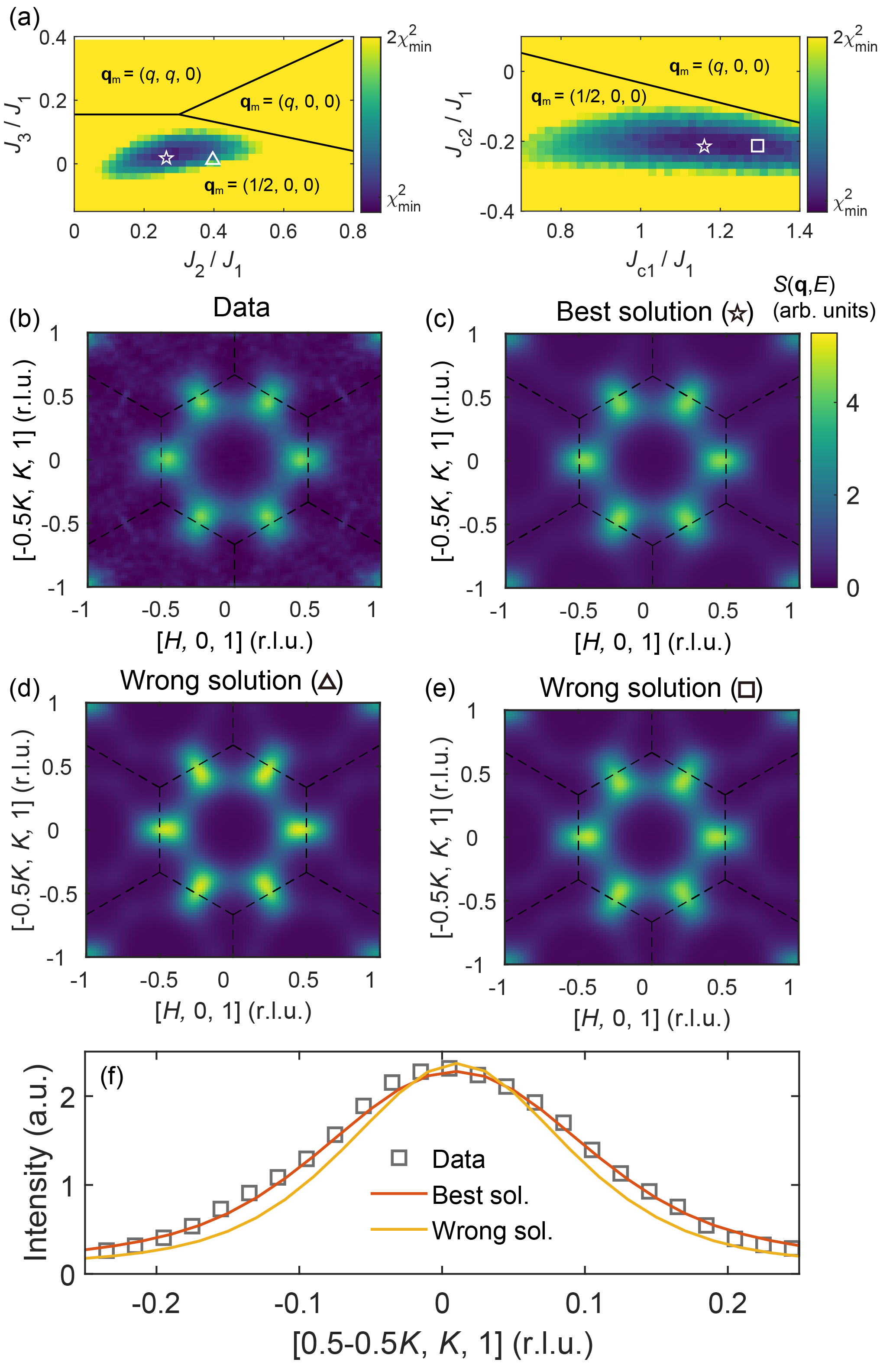
Figure 9: Comparing paramagnetic excitation spectra obtained from multiple exchange parameter sets that yield different level of goodness-of-fit (i.e., $\chi^{2}$ metric). (a) The same color plots as Figs. 2(k)–(l), which additionally marks two parameter sets (a white square and triangle) possessing worse $\chi^{2}$ than the optimal solution (a white star). (b) The same color plot as Fig. 3(a). (c)–(e) Corresponding LLD spectra obtained from the three different parameter sets indicated in (a). (f) A vertical cut of the constant-$\omega$ spectra in (b)–(d). Error bars are much smaller than the data symbol.

Appendix E Temperature-dependent magnetic ground state revealed by classical Monte Carlo simualtions

Finite-temperature magnetic ground states of our optimal spin model (see Table 1) with finite $K>0$ were investigated using classical Monte Carlo simulations, combined with the LLD equation and simulated annealing technique. We created a $30\times 30\times 8$ sized Co1/3TaS2 supercell (14,400 Co sites) and sampled its time evolution at each temperature point while cooling down the system from 50 K to 5 K. The Langevin time step ($\mathrm{d}t$) and damping constant were set to 0.02 meV^-1 and 0.1, respectively. Each temperature was sampled over 512,000 Langevin time steps. From the collected samples, we calculated staggered magnetization and scalar spin chirality using the equations below, which represent an order parameter for the stripe single-${\mathbf{Q}}$ and tetrahedral triple-${\mathbf{Q}}$ magnetic orderings, respectively:

$$M_{\mathrm{stagg}}=\frac{1}{N}\sum_{i}{(-1)^{2\pi(\mathbf{q}^{\nu}_{\mathrm{m}}\cdot\mathbf{r}_{i})}\langle\mathbf{S}_{i}\rangle},$$ (19)

$$\chi_{ijk}=\frac{\sum_{\Delta}{\langle\mathbf{S}_{\Delta 1}\cdot(\mathbf{S}_{\Delta 2}\times\mathbf{S}_{\Delta 3})\rangle}}{N_{t}},$$ (20)

where $i$ is a Co site index, $\Delta$ indexes a single triangular plaquette on a Co triangular lattice consisting of three sites ($\Delta 1$, $\Delta 2$, $\Delta 3$), $\mathbf{q}^{\nu}_{\mathrm{m}}$ ($\nu=1,2,3$) is three possible ordering wave vectors for the stripe single-${\mathbf{Q}}$ order, and $N$ ($N_{t}$) is the total number of spins (triangular plaquettes). We used S = 3/2 for the simulations.

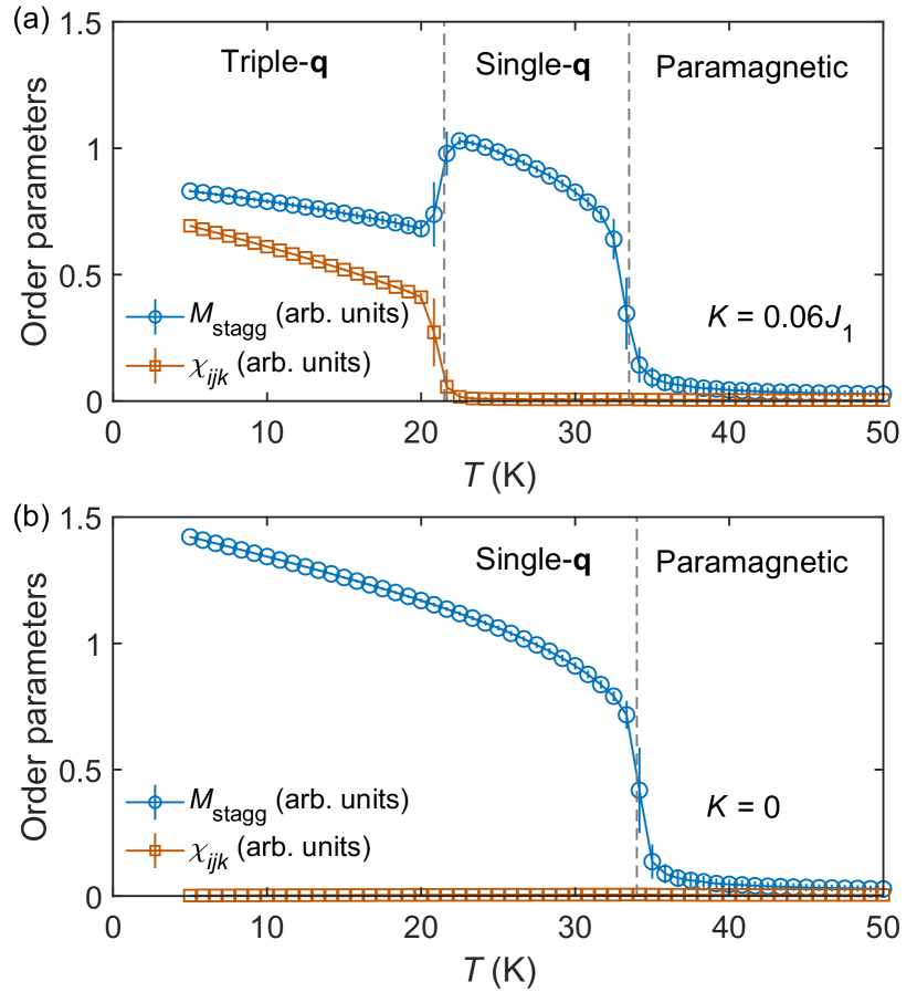
Figure 10: Temperature-dependent staggered magnetization ($M_{\mathrm{stagg}}$) and scalar spin chirality calculated by classical Monte-Carlo simulations. The bilinear exchange parameters in Table 1 are used for the calculation. Panel (a) [panel (b)] shows the result with $K=0.06J_{1}$ ($K=0)$.

Fig. 10(a) shows the resultant temperature-dependent order parameters obtained with finite $K$. Our optimal exchange parameter set yields $T_{\mathrm{N}1}$ = 34 K very close to the experimental observation $T_{\mathrm{N}1}$ = 38 K, again supporting our solution in addition to other features described Appendix D. Moreover, $K=0.06J_{1}=0.07$ meV reproduces not only the two-step transition process illustrated in Fig. 1(a) but also its quantitative interval $T_{\mathrm{N}1}$/$T_{\mathrm{N}2}$ = 0.7. Thus, the LLD simulations with $K=0.06J_{1}$ successfully provide the triple-${\mathbf{Q}}$ and single-${\mathbf{Q}}$ spin dynamics at 5 K and 30 K, enabling a direct comparison with our experimental data.

For comparison, we also plotted the results without $K$ in Fig. 10(b). As expected, the single-${\mathbf{Q}}$ stripe ordering becomes the magnetic ground state. Notably, this outcome is not captured in a simple classical energy comparison, as the single-${\mathbf{Q}}$ and triple-${\mathbf{Q}}$ states are simply degenerate. However, thermal fluctuations break this degeneracy in both the simulation and reality.

Appendix F Parameter-dependent anisotropy of $v_{\mathrm{L}}(\mathbf{k})$

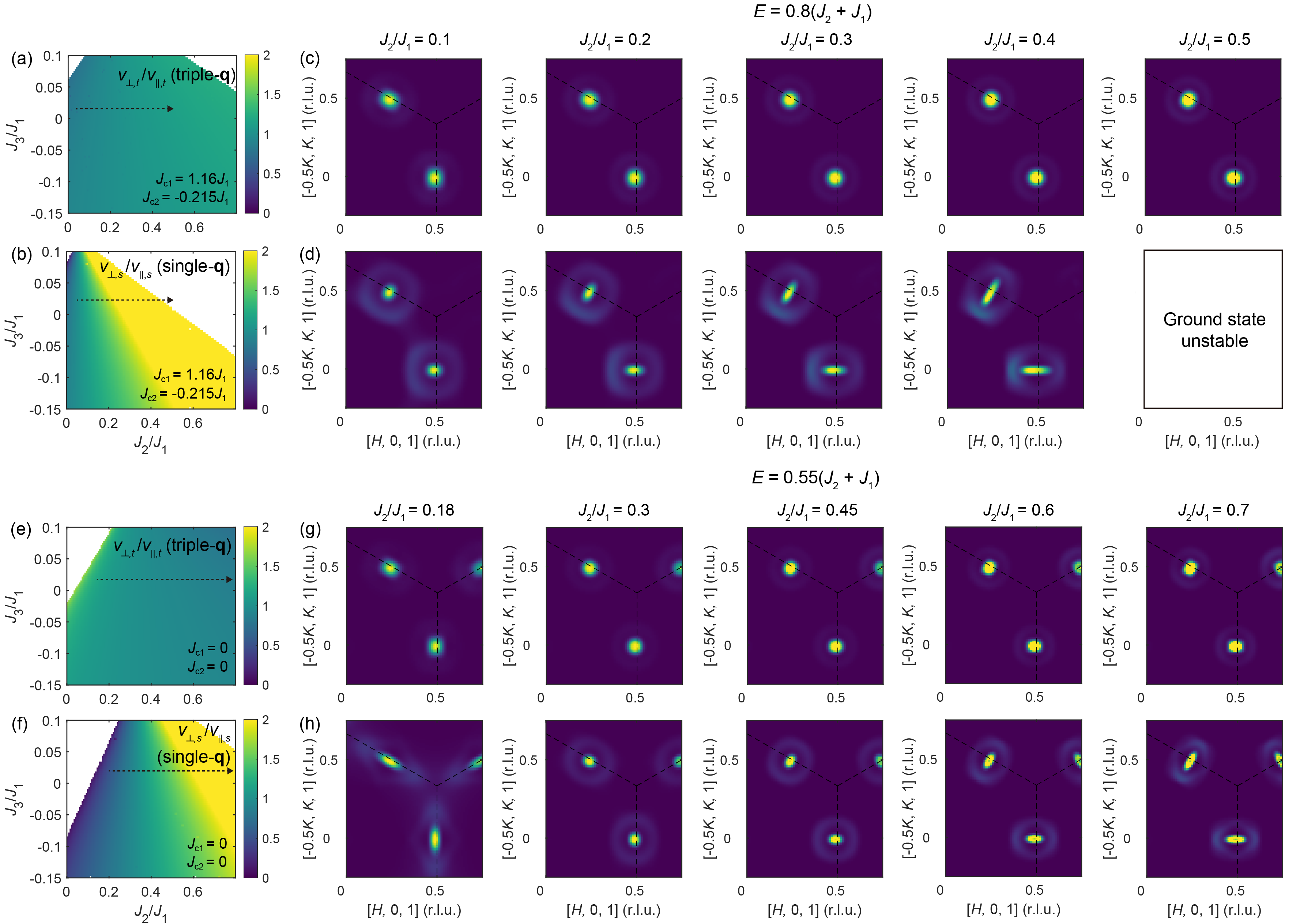
Figure 11: Visualizing characteristic patterns of the constant-$\omega$ cut stemming from the anisotropic $v_{\mathrm{L}}(\mathbf{k})$. (a)–(b) Parameter-dependent anisotropy of $v_{\mathrm{L}}(\mathbf{k})$ for the triple-${\mathbf{Q}}$ and single-${\mathbf{Q}}$ phases, quantified by $v_{\perp}/v_{\parallel}$ [same as the plots shown in Fig. 4(a)–(b)]. (c)–(d) Constant-$\omega$ cuts of the triple-${\mathbf{Q}}$ and single-${\mathbf{Q}}$ magnon spectrum at $\hbar\omega=0.8(J_{2}+J_{1})$ from several different $J_{2}/J_{1}$. They visualize individual $v_{\perp}/v_{\parallel}$ as an eccentricity of the linear magnon’s signal at the M Points. (e)–(h) Same as (a)–(d), but based on the spin model without any interlayer interactions $J_{\mathrm{c1}}$ and $J_{\mathrm{c2}}$.

Figure 12: A marginal effect of $K$ on theoretical $v_{\perp}/v_{\parallel}$. (a)–(b) $J_{2}$ and $J_{3}$ dependence of $v_{\perp}/v_{\parallel}$ for the triple-${\mathbf{Q}}$ and single-${\mathbf{Q}}$ phase with finite $K$, respectively. Note that we used an opposite sign of $K$ for each calculation to stabilize the magnetic ground state. (c)–(d) The same calculation result as (a)–(b), but without finite $K$.

In this section, we provide a more detailed analysis of the parameter dependence of $v_{\mathrm{L}}(\mathbf{k})$. First, Fig. 11 visualizes the consequence of contrasting $v_{\mathrm{L}}(\mathbf{k})$ between the stripe single-${\mathbf{Q}}$ and tetrahedral triple-${\mathbf{Q}}$ orderings through constant-$\omega$ cuts at low energies. Indeed, different profiles of $v_{\mathrm{L}}(\mathbf{k})$ across most of the parameter space generally result in distinct constant-$\omega$ spectra for these two magnetic ground states [Fig. 11(a)–(b)]. This contrast remains clear even without interlayer interactions [i.e. 2D limit, Fig, 11(e)–(f)]. However, $v_{\mathrm{L}}(\mathbf{k})$ of these two magnetic orderings can coincidentally be very similar for specific parameter sets, e.g., $J_{2}/J_{1}=0.3$ in Fig. 11(g)–(h). Thus, even though the likelihood is low, caution is advised when analyzing $v_{\mathrm{L}}(\mathbf{k})$ to distinguish single-${\mathbf{Q}}$ and triple-${\mathbf{Q}}$ magnetic structures if the exchange parameter set of a system, derived independently from the spin-wave analysis, happens to lie in such a region.

We also examine the effect of $K$ on $v_{\mathrm{L}}(\mathbf{k})$, in addition to the effect of interlayer interactions shown in Fig. 4. Fig. 12 compares $v_{\perp,t}/v_{\parallel,t}$ and $v_{\perp,s}/v_{\parallel,s}$ calculated with and without finite $K$. For the the single-${\mathbf{Q}}$ phase calculation, we used $K<0$ to ensure its stabilization. The magnitude of $K$ was set to 0.06$J_{1}$, as determined from reproducing $T_{\mathrm{N}2}$/$T_{\mathrm{N}1}$ = 0.6 in classical Monte Carlo simulations (see Appendix E).

The results show that $K$ has a very marginal effect on the momentum dependence of $v_{\mathrm{L}}(\mathbf{k})$. Unlike $J_{\mathrm{c1}}$ and $J_{\mathrm{c2}}$, $K$ hardly changes the parameter dependence of $v_{\perp,t}/v_{\parallel,t}$ [Fig. 12(a) and 12(c)]. Also, the variation of $v_{\perp,s}/v_{\parallel,s}$ due to $J_{2}$ and $J_{3}$ remains qualitatively the same, except for a uniform shift toward the right when adding $K=-0.06J_{1}$. We attribute this outcome primarily to the smaller magnitude of $K$ compared to bilinear exchange parameters. Such an order-of-magnitude smaller $K$ is expected to arise in most materials, considering its higher-order nature. Thus, $K$ or other four-spin interactions generally would not play a significant role in determining the momentum dependence of $v_{\mathrm{L}}(\mathbf{k})$ for both single-${\mathbf{Q}}$ and triple-${\mathbf{Q}}$ orderings. Consequently, refining only bilinear exchange interactions in the paramagnetic phase still leads to the successful identification of single-${\mathbf{Q}}$ and triple-${\mathbf{Q}}$ magnetic orderings by comparing the resultant $v_{\mathrm{L}}(\mathbf{k})$.

Appendix G Dynamical susceptibility and dynamical structure factor

When analyzing a spin-wave spectrum with sizable thermal fluctuations, it can sometimes be useful to visualize the dynamical susceptibility [$\chi^{\prime\prime}(\mathbf{q},\omega)$] instead of the dynamical structure factor [$S(\mathbf{q},\omega)$] [36]. $\chi^{\prime\prime}(\mathbf{q},\omega)$ can be easily calculated from $S(\mathbf{q},\omega)$ through the following equation:

$$\chi^{\prime\prime}(\mathbf{q},\omega)=\pi(1-e^{-\hbar\omega/k_{\mathrm{B}}T})\times S(\mathbf{q},\omega),$$ (21)

where $T$ is the measurement or LLD simulation temperatures. This conversion effectively deconvolutes the Bose factor $\frac{1}{\pi(1-e^{-\hbar\omega/k_{\mathrm{B}}T})}$ and removes an increased spectral weight in the low-$E$ region due to thermal excitations, which often conceals the low-energy structure of the magnetic excitations in the color plot of $S(\mathbf{q},\omega)$. However, it is important to note that the INS data measured at 5 K (i.e., the triple-${\mathbf{Q}}$ phase) show no noticeable different between $\chi^{\prime\prime}(\mathbf{q},\omega)$ and $S(\mathbf{q},\omega)$, as the thermal energy at 5 K is marginal compared to the energy of the magnon spectrum (see Fig. 5).

Appendix H Linewidth broadening and renormalization of magnon branches

We describe in more detail the evidence suggesting intrinsic magnon linewidth broadening (i.e., magnon decay) and renormalization beyond LSWT in Co1/3TaS2. The most unambiguous way to demonstrate intrinsic magnon linewidth broadening is to compare a magnon spectrum to a phonon spectrum measured in the same experiment. Except for a few special cases, phonons typically have a fairly long lifetime and thus represent a reference spectrum broadened only by instrumental resolution. Thus, a magnon spectrum that is significantly broader than the phonon signal directly indicates a finite magnon lifetime. Indeed, Fig. 13 shows that the magnon spectrum of Co1/3TaS2 is much broader than its phonon spectrum, indicating the prevalence of magnon decay channels over a wide energy-momentum space. Meanwhile, analyzing the intrinsic linewidth broadening quantitatively (e.g., its momentum dependence) is very challenging due to the complex resolution ellipsoid of the time-of-flight spectrometer [54].

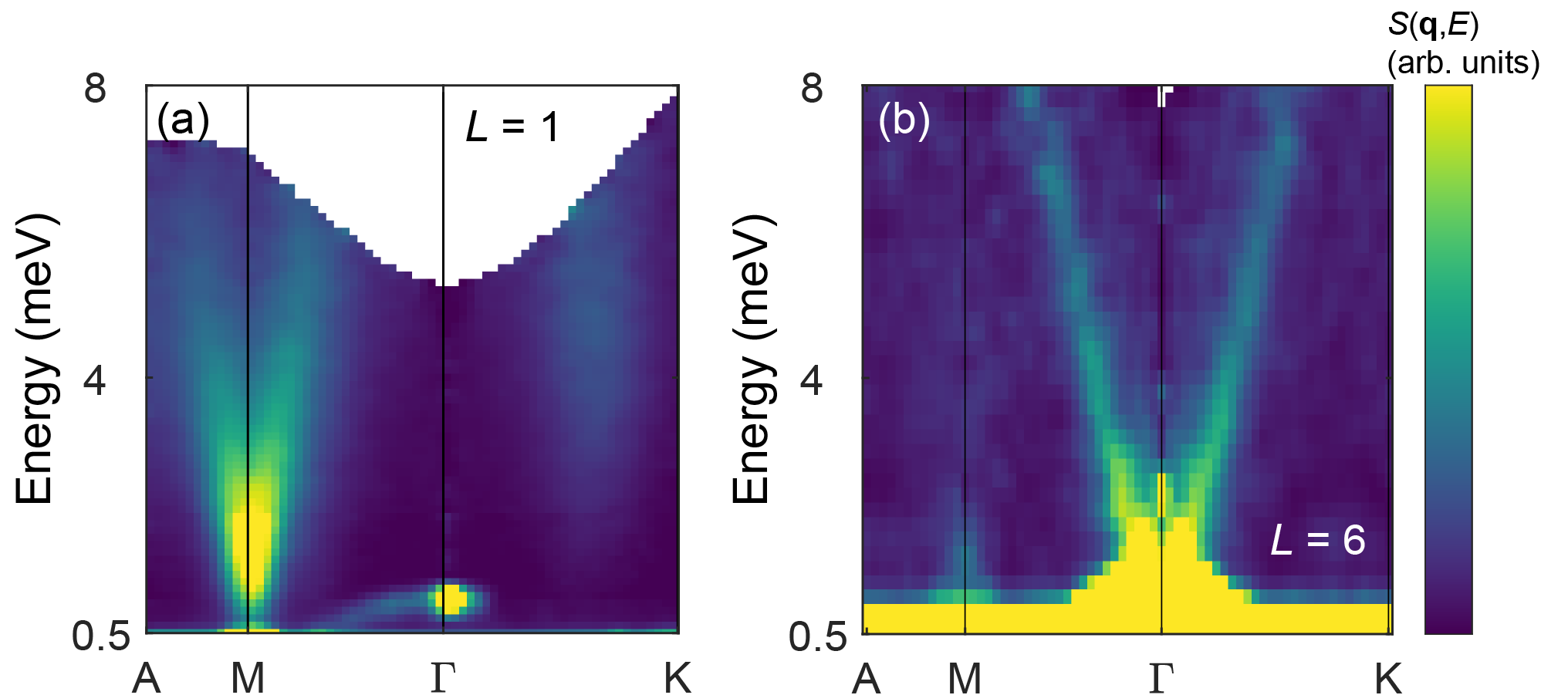
Figure 13: Two energy-momentum slices of the INS data ($T=5$ K) from different Brillouin zones. (a) A data slice on the [HK1] plane (low-${\mathbf{q}}$), showing a magnon spectrum. (b) A data slice on the [HK6] plane (high-${\mathbf{q}}$), showing a phonon spectrum. The phonon spectrum is much sharper than the magnon spectrum, indicating the presence of intrinsic linewidth broadening for the magnon modes in Co1/3TaS2.

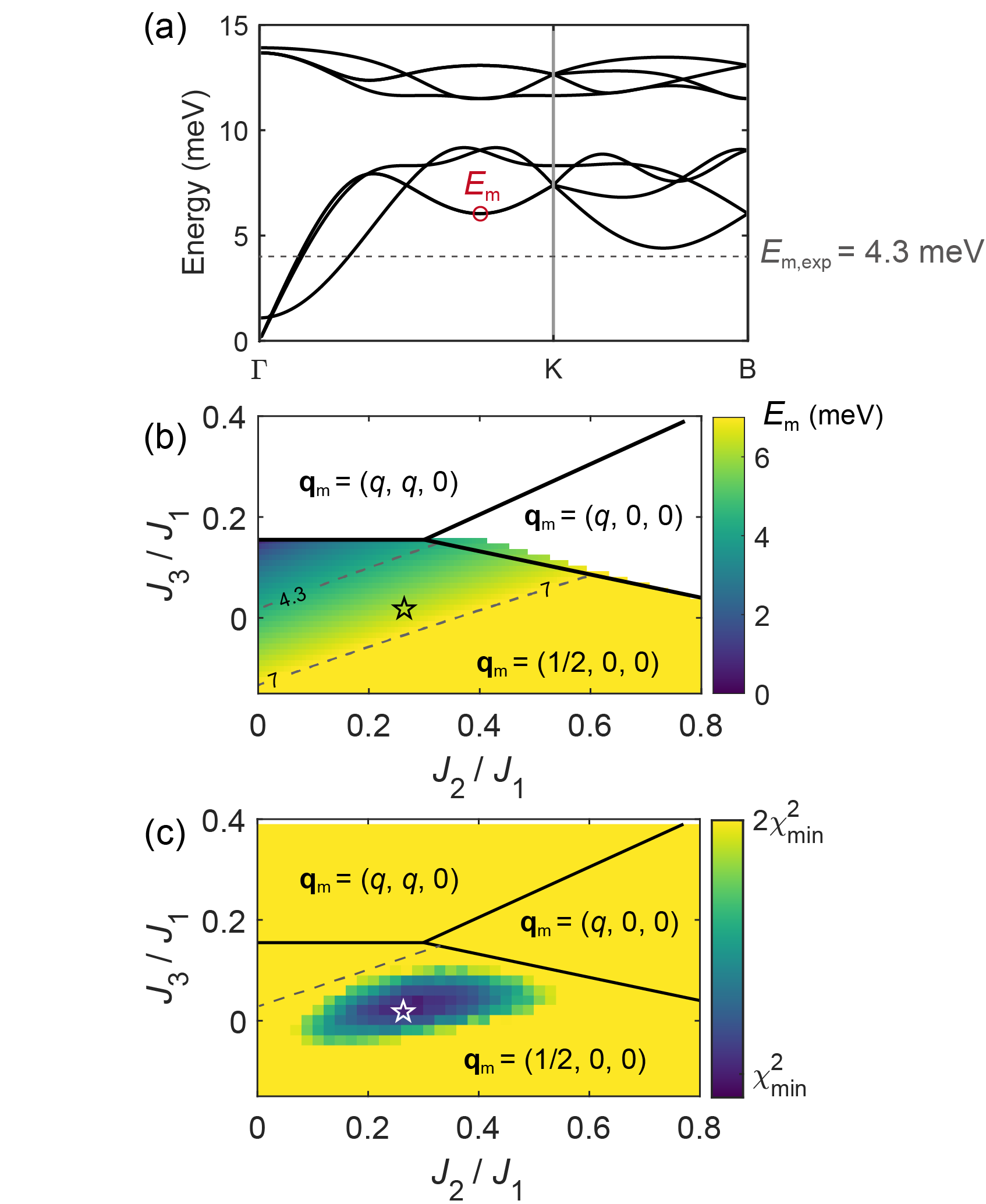
Figure 14: Failure of LSWT in describing the observed magnon spectrum of Co1/3TaS2 in the triple-${\mathbf{Q}}$ phase. (a) The magnon dispersion of the tetrahedral triple-${\mathbf{Q}}$ phase calculated using LSWT with the parameters in Table 1 and $K=0.06J_{1}$. The red circle in (a) denotes the lowest magnon eigenvalue ($E_{\mathrm{m}}$) at ${\mathbf{Q}}$ = $\mathbf{q}_{\alpha}$ [see Figs. 6(c)] where the magnon dispersion forms a local minimum. The dashed grey line in (a) indicates the experimental $E_{\mathrm{m}}$ [Fig. 6(d)]. (b) $J_{2}/J_{1}$ and $J_{3}/J_{1}$ dependence of $E_{\mathrm{m}}$. The dashed grey lines in (b) are the trajectory of $E_{\mathrm{m}}=4.3$ and 7 meV. (c) The goodness-of-fit map ($\chi^{2}$ metric) from the paramagnetic phase analysis (Fig. 2), plotted in the same axes ranges as (b). The dashed grey line in (c) is the trajectory of $E_{\mathrm{m}}=4.3$ meV.

The magnon energy renormalization suggested at $\mathbf{q}_{\alpha,\beta,\gamma}$ in the triple-${\mathbf{Q}}$ phase (see the main text) is further supported by our advanced analysis illustrated in Fig. 14. Fig. 14(b) shows $J_{2}/J_{1}$ and $J_{3}/J_{1}$ dependence of the lowest magnon eigenvalue at ${\mathbf{q}}$ $=\mathbf{q}_{\alpha}$ calculated by LSWT for the triple-${\mathbf{Q}}$ ordering [$E_{\mathrm{m}}$, see Fig. 14(a)], where we used $J_{1},J_{\mathrm{c1}},$ and $J_{\mathrm{c2}}$ shown in Table 1. The optimal parameter set is different from those yielding $E_{\mathrm{m}}=4.3$ meV observed experimentally [Fig. 6((d))]. Notably, the parameter sets that produce $E_{\mathrm{m}}=4.3$ meV [the dashed lines with the number 4.3 in Fig. 14(b)] exhibits a very poor $\chi^{2}$-metric (=$2.8\chi^{2}_{\mathrm{min}}$) in the paramagnetic excitation analysis [Fig. 14(c)]. This metric is much worse than that of the parameter sets that already show apparent disagreement with the measured $S(\mathbf{q},\omega)$ (see Fig. 9 in Appendix D). Moreover, using the parameter sets that give $E_{\mathrm{m}}=4.3$ meV introduces additional discrepancies between the measured and simulated spectra at momentum positions other than $\mathbf{q}=\mathbf{q}_{\alpha}$. Thus, the observed $E_{\mathrm{m}}=4.3$ meV at $\mathbf{q}=\mathbf{q}_{\alpha}$ suggests the presence of magnon energy renormalization beyond LSWT, which indeed could be present in the triple-${\mathbf{Q}}$ phase of Co1/3TaS2 as described in the main text.

Appendix I Magnon decay/renormalization by the Stoner continuum

In the main text, we suggested that the pronounced magnon decay/renormalization observed on the edges of the hexagon that connects the M points in the momentum space (${\mathbf{q}}\in\{\mathbf{q}_{h}\}$) is primarily attributed to the two-magnon continuum. Nevertheless, the Stoner continuum may also partially contribute to our observations. This is because, for metallic antiferromagnets with a Fermi surface lying at ${\mathbf{q}}\in\{\mathbf{q}_{h}\}$, a gapless Stoner continuum should be present at ${\mathbf{q}}\in\{\mathbf{q}_{h}\}$. Notably, the Fermi surface of Co1/3TaS2 is close to this condition [25].

Fig. 15(a) illustrates the decay of a magnon into a spin-flip electron-hole pair around the Fermi energy ($E_{\mathrm{F}}$), where both the electron and hole are on the same band index. Such intraband spin-flip excitations can occur in antiferromagnets that retain the spin degeneracy of electron bands (mostly due to $PT$ symmetry). Thus, for momentum vectors $\mathbf{k}$ that connect two different positions on the Fermi level, a Stoner excitation process with momentum transfer $\mathbf{k}$ can occur with infinitesimally small energy transfer. In other words, a gapless Stoner continuum is present at $\mathbf{k}$, allowing magnons with ${\mathbf{q}}=\mathbf{k}$ and any finite energy to decay. Fig. 15(b) shows that when the Fermi surface lies on ${\mathbf{q}}\in\{\mathbf{q}_{h}\}$, any momentum vectors on $\mathbf{q}_{h}$ satisfies this condition. Thus, a gapless Stoner continuum is expected along ${\mathbf{q}}\in\{\mathbf{q}_{h}\}$, potentially leading to sizable decay and renormalization of magnons at these momentum positions, such as $\mathbf{q}_{\alpha}$ in Fig. 6. A more quantitative understanding of the effects of the Stoner continuum would require calculating the Stoner continuum DOS based on the full electron band structure of Co1/3TaS2 (e.g. see [54]), which is beyond the scope of this study.

However, it is important to note that the magnon decay process via the Stoner continuum could be more complex in non-collinear magnets than the simple conjecture described above. A noncollinear spin configuration complicates the spin index of electron bands in momentum space (rather than simply spin-up or spin-down, the spin index will also be non-collinear), which would affect the Stoner excitation process as it involves a full flip of a single spin [54]. This complication would suppress the intraband Stoner excitation processes to some extent and potentially remove some magnon decay channels discussed in the previous paragraph.

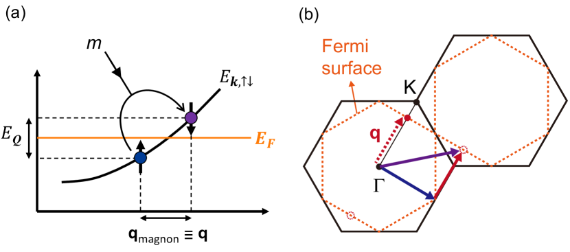
Figure 15: (a) Schematic illustration of a spin-flip electron-hole pair creation (i.e., a Stoner excitation) in a metallic antiferromagnet with spin-degenerate electron band structure. (b) The Stoner excitation process with momentum transfer $\mathbf{Q}\in\{\mathbf{q}_{h}\}$ and infinitesimally small energy transfer for a three-quarter-filled Fermi surface geometry. In this situation, the Stoner continuum becomes gapless at $\mathbf{Q}\in\{\mathbf{q}_{h}\}$.