The non-perturbative adiabatic invariant is all you need

Abstract

Perturbative guiding center theory adequately describes the slow drift motion of charged particles in the strongly-magnetized regime characteristic of thermal particle populations in various magnetic fusion devices. However, it breaks down for particles with large enough energy. We report on a data-driven method for learning a non-perturbative guiding center model from full-orbit particle simulation data. We show the data-driven model significantly outperforms traditional asymptotic theory in magnetization regimes appropriate for fusion-born $\alpha$-particles in stellarators, thus opening the door to non-perturbative guiding center calculations.

In contrast to tokamaks, which rely on strongly self-organized plasma states for confinement, stellarators achieve confinement predominantly through application of external magnetic fields generated by highly optimized three-dimensional current-carrying coils. This confinement method affords plasma relatively few opportunities to tap free energy sources that lead to deleterious instabilities. But greater stability comes at the price of complicated particle confinement theory. The theory is so complex that early stellarators failed to compete with their tokamak counterparts. Modern understanding of quasisymmetric Bo2_1983 ; NZ_1988 ; Burby_phase_2013 ; Helander_review_2014 ; BKM_2020 ; Rodriguez_2020 , omnigeneous Hall_1975 ; Helander_review_2014 ; Landreman_2012 ; Parra_2015 , quasi-isodynamic QI_2023 , and isodrastic BMN_2023 magnetic fields provides practical optimization metrics that lead to stellarator designs with confinement quality for thermal plasma comparable to tokamaks. However, as we will show, these metrics cannot be trusted for $3.5\text{ MeV}$ fusion-born $\alpha$-particles.

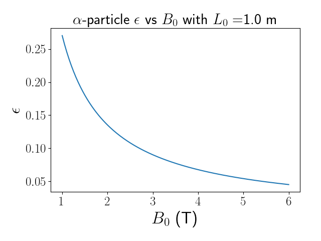
Figure 1: Fusion-born $\alpha$-particle $\epsilon=\rho_{0}/L_{0}$ vs magnetic field strength $B_{0}$ in a device with scale length $L_{0}=1\,\text{m}$

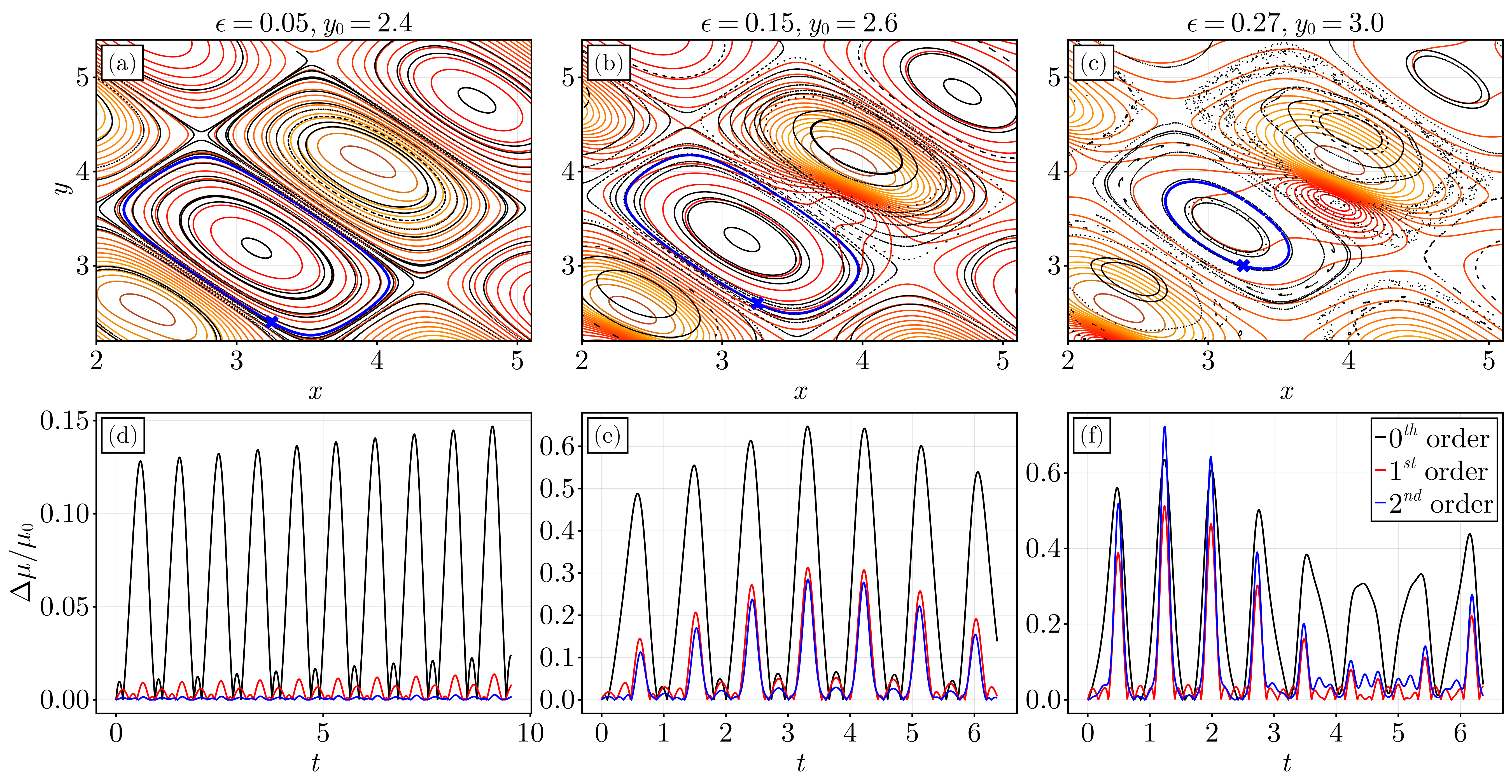
Figure 2: (Top) Poincaré sections ($z=v_{z}=v_{y}=0,v_{x}>0$) of the full-orbit dynamics of Eq. (1) (black) and level sets of an adiabatic invariant truncation (color) for different values of $\epsilon$. Second-order truncation is used in (a); first-order truncation is used in (b) and (c). (Bottom) Relative error time traces of three truncations of adiabatic invariant series for the same $\epsilon$ values. Underlying trajectories are denoted by a blue cross in (a)-(c).

All of advanced stellarator confinement theory assumes that an asymptotic expansion, known as the guiding center model Kruskal_1962 ; Littlejohn_1981 ; Littlejohn_1983 ; Littlejohn_1984 ; Cary_2009 ; Burby_loops_JMP , adequately describes dynamics of any given plasma particle. The dimensionless parameter $\epsilon=\rho_{0}/L_{0}$, equal to the ratio of a particle’s gyroradius $\rho_{0}$ to the scale length of the magnetic field $L_{0}$, measures the quality of this assumption; smaller values of $\epsilon$ imply greater accuracy. The gyroradius of a fusion-born $\alpha$ is 19.6 times larger than that of a triton in $10\text{ keV}$ burning magnetized plasma. Thus, traditional guiding center theory always describes $\alpha$-dynamics somewhat less accurately than thermal particle dynamics. While this observation alone need not cause concern, numerical study of $\alpha$-particle trajectories with $\epsilon$ in the realistic range shown in Fig. 1 suggests a serious issue as well as an exciting theoretical opportunity.

For particles with $\epsilon\in\{0.05,0.15,0.27\}$ (cf. Fig. 1) moving in the simple $z$-symmetric field geometry $\bm{B}=B(x,y)\,\bm{e}_{z}$, where

$$B(x,y)=1+\sum_{i=1}^{2}a_{i}\,\cos(k_{xi}\,x+k_{yi}\,y),$$ (1)

$$k_{x1}=k_{y2}=3,\quad k_{y1}=k_{x2}=1,\quad a_{1}=a_{2}=.3,$$

the leading-order perturbative adiabatic invariant $\mu_{0}={m\,v_{\perp}^{2}}/{(2|\bm{B}|)}$ suffers strikingly-large variations in time. Worse yet, for $\epsilon\in\{0.15,0.27\}$, when $\mu_{0}$ is replaced with higher-order asymptotic corrections Burby_gc_2013 conservation need not improve, indicating collapse of the adiabatic invariant’s optimal truncation order Berry_1991 . See Fig. 2. It follows that the guiding center asymptotic expansion may grossly mischaracterize $\alpha$-particle trajectories in today’s stellarator optimization codes. On the other hand, the phase portraits in Fig. 2 reveal that a large fraction of $\alpha$ trajectories do enjoy an adiabatic invariant, even though it cannot be captured using standard guiding center theory; its level sets coincide with the invariant circles in the phase portrait. (Note there is probably no true smooth invariant, even for $\epsilon\in\{0.05,0.15\}$, due to presence of very thin chaotic bands.) This suggests there may yet be a good notion of adiabatic invariant, and perhaps even guiding center dynamics, for $\alpha$’s that break the traditional guiding center model. Whatever that notion may be, collapse of the optimal truncation order indicates it lies beyond the reach of traditional asymptotic expansions.

In this Letter we describe a non-perturabative guiding center model suitable for $\alpha$-particles in stellarators. First we deduce non-perturbative guiding center equations of motion assuming the non-perturbative adiabatic invariant $\mathcal{J}$ is known. Remarkably, these equations are completely determined by first-order derivatives of $\mathcal{J}$ and the magnetic field. They enjoy a Hamiltonian structure comparable with that of the usual asymptotic theory Littlejohn_1981 . Then we describe a data-driven method for learning $\mathcal{J}$ from a dataset of full-orbit $\alpha$-particle trajectories. We apply this method to $\alpha$ dynamics in the fields underlying Fig. 2 and find that the non-perturbative guiding center model determined by our learned $\mathcal{J}$ significantly outperforms the standard guiding center expansion. Our work establishes the need for a non-perturbative adiabatic invariant that can be applied in any magnetic field configuration; the method of finding $\mathcal{J}$ reported here can only be applied on a per-magnetic-field basis. The fact that such a general-purpose adiabatic invariant exists in the perturbative regime suggests a non-perturbative general-purpose adiabatic invariant may exist as well.

In a seminal paper, Kruskal Kruskal_1962 showed that the traditional guiding center expansion originates from a hidden perturbative $U(1)$-symmetry found in the ordinary differential equations describing single-particle motion, $X=\dot{\bm{x}}\cdot\partial_{\bm{x}}+\dot{\bm{v}}\cdot\partial_{\bm{v}}$, where $\dot{\bm{v}}=\bm{v}\times\bm{B}$ and $\dot{\bm{x}}=\epsilon\,\bm{v}$. He dubbed the infinitesimal generator of the perturbative hidden symmetry the roto rate $R$ and showed that its formal expansion in powers of $\epsilon$ is uniquely determined to all orders, with first term given by $R_{0}=\bm{v}\times\bm{b}\cdot\partial_{\bm{v}}$.

Our non-perturbative guiding center model assumes (I) existence of a non-perturbative $U(1)$-symmetry with infinitesimal generator $\mathcal{R}$ such that $\mathcal{R}|_{\epsilon=0}=R_{0}$. We refer to streamlines of $\mathcal{R}$ as $U(1)$-orbits. Here symmetry means the non-perturbative roto rate $\mathcal{R}$ is a Hamiltonian vector field with Hamiltonian function $\mathcal{J}$ that commutes with the kinetic energy $E=|\bm{v}|^{2}/2$ under the Lorentz force Poisson bracket,

$$\{F,G\}=\bm{B}\cdot\partial_{\bm{v}}F\times\partial_{\bm{v}}G+\epsilon\,(\partial_{\bm{x}}F\cdot\partial_{\bm{v}}G-\partial_{\bm{x}}G\cdot\partial_{\bm{v}}F),$$

i.e. $\{E,\mathcal{J}\}=0$. We will refer to $\mathcal{J}$ as the non-perturbative adiabatic invariant.

To ensure topological similarity with the known $U(1)$-symmetry at $\epsilon=0$, we also assume (II) that each $U(1)$-orbit generated by $\mathcal{R}$ transversally intersects a certain phase space Poincaré section $\Sigma$ exactly once. To define $\Sigma$, introduce phase space coordinates $(\bm{x},v_{\parallel},v_{\perp},\zeta)$ such that $\bm{v}=v_{\parallel}\,\bm{b}+v_{\perp}\,(\cos\zeta\bm{e}_{1}+\sin\zeta\bm{e}_{2})$. Here $\bm{e}_{1},\bm{e}_{2}$ are unit vector fields chosen to ensure $(\bm{e}_{1},\bm{e}_{2},\bm{b})$ is a right-handed orthonormal frame. Then set $\Sigma=\{(\bm{x},v_{\parallel},v_{\perp},0)\}$. We will refer to $\Sigma$ as the guiding center Poincaré section.

Since $\mathcal{R}|_{\epsilon=0}=R_{0}=-\partial_{\zeta}$, (I) $\Rightarrow$ (II) when $\epsilon=0$. Due to persistence of transversal intersections under deformations GP_1974 , (I) $\Rightarrow$ (II) for $\epsilon$ in some open interval $(-\epsilon_{0},\epsilon_{0})$, $\epsilon_{0}>0$, and $v_{\perp}$ not too close to $0$. However, (II) is still essential because we cannot predict $\epsilon_{0}$ in advance.

Intrinsically, a particle’s guiding center is equal to the $U(1)$-orbit passing through that particle’s phase space location. Guiding center phase space is therefore intrinsically the collection of all $U(1)$-orbits. Constructing a guiding center model, perturbative or non-perturbative, requires equipping this space with coordinates and identifying an evolution law for $U(1)$-orbits in that coordinate system. Traditional guiding center theory painstakingly constructs such coordinates order-by-order in $\epsilon$, resulting in non-unique model equations with exploding complexity that cannot be applied in the non-perturbative regime identified in Fig. 2.

Breaking with tradition, we coordinatize $U(1)$-orbits by assigning to each orbit its point of intersection with $\Sigma$, $(\bm{x},v_{\parallel},v_{\perp},\zeta)=(\bm{X},u,r,0)$. In this manner we regard $\Sigma$ as a concrete realization of the abstract space of $U(1)$-orbits. We will use $\pi$ to denote the map that sends each particle-space point $(\bm{x},v_{\parallel},v_{\perp},\zeta)$ to its $U(1)$-orbit-mate on $\Sigma$, $\pi(\bm{x},v_{\parallel},v_{\perp},\zeta)=(\bm{X},u,r)$. We will refer to $\pi$ as the footpoint map and the image of $(\bm{x},v_{\parallel},v_{\perp},\zeta)$ under $\pi$ as that phase point’s footpoint. Note that $\pi(\bm{x},v_{\parallel},v_{\perp},0)=(\bm{x},v_{\parallel},v_{\perp})$, indicating that a particle’s footpoint coincides with its phase space location whenever the particle’s trajectory intersects $\Sigma$. We define the guiding center of any particle as that particle’s footpoint on $\Sigma$.

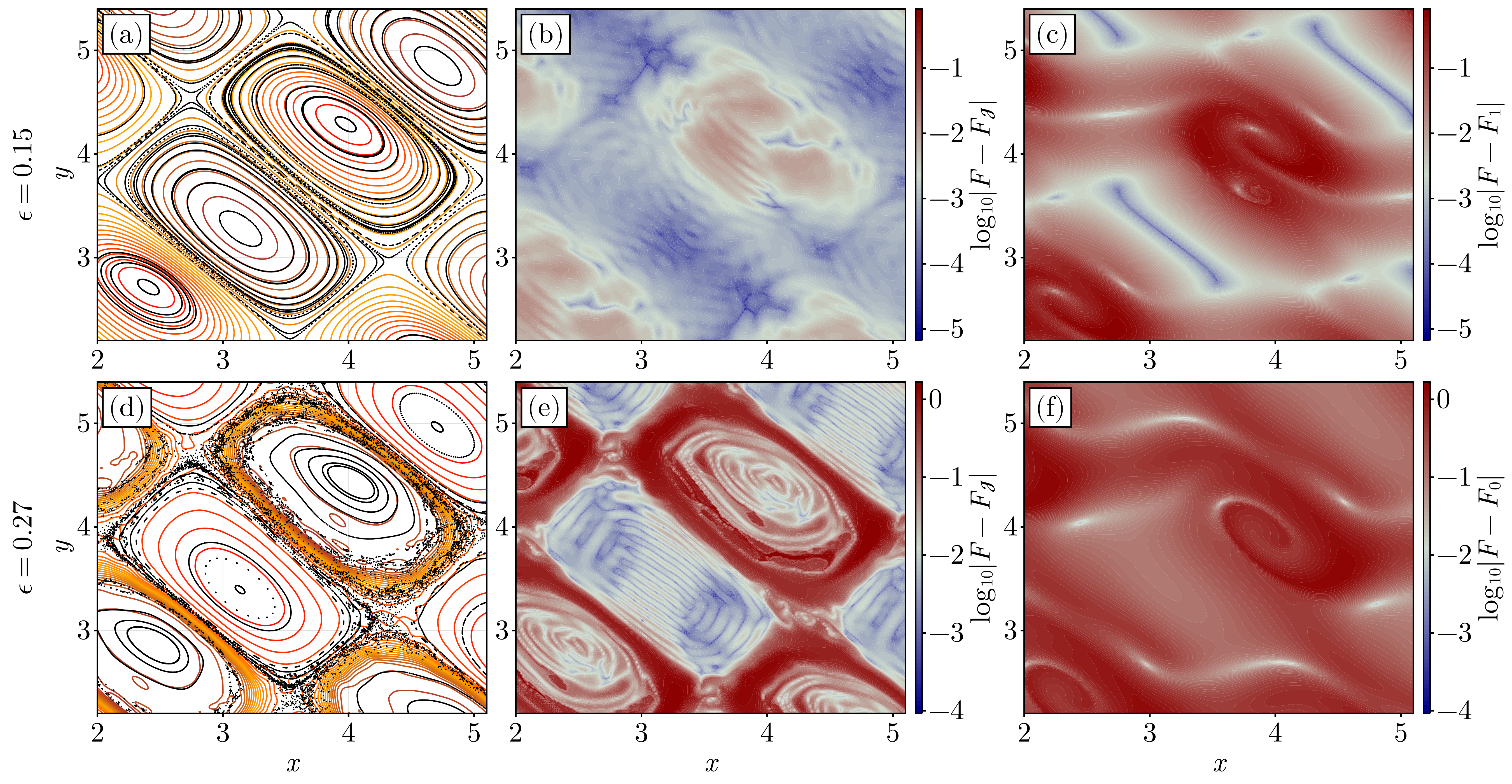
Figure 3: (a,d) Poincaré sections of the full-orbit dynamics (black) and level sets of the learned $\mathcal{J}_{\Sigma}$ (color) for $\epsilon\in\{0.15,0.27\}$ (cf. Fig. 2 (b,c)). (b,e) Error of $\mathcal{J}_{\Sigma}$ prediction of the dynamics from the full-orbit dynamics over a gyroperiod. (c,f) Error of the order-$j$ truncated dynamics (4) over a gyroperiod with $j=(1,0)$.

As a particle moves through phase space its footpoint traces an image curve on $\Sigma$. Because the Lorentz force equations of motion are $U(1)$-invariant by hypothesis that image curve is a streamline for a uniquely defined vector field on $\Sigma$, $X_{\Sigma}=\dot{\bm{X}}\cdot\partial_{\bm{X}}+\dot{u}\,\partial_{u}+\dot{r}\,\partial_{r}$. See Theorem 1 in supplementary material. We refer to $X_{\Sigma}$ as the footpoint flow field. By identifying $\Sigma$ with the space of $U(1)$-orbits we identify footpoint dynamics with $U(1)$-orbit dynamics as a byproduct. Thus, the components of the footpoint flow field define the non-perturbative guiding center equations of motion. We identify explicit formulas for these components involving only $\mathcal{J}$, $\bm{B}$, and the unit vectors $\bm{e}_{1},\bm{e}_{2}$ as follows.

Any pair of functions $f,g$ on $\Sigma$ determines a pair of $U(1)$-invariant functions $F=f\circ\pi$, $G=g\circ\pi$ on all of phase space by precomposing with the footpoint map. Because $\mathcal{R}$ is a Hamiltonian vector field the function $\{F,G\}$ is also $U(1)$-invariant. It follows that the restriction $\{f,g\}_{\Sigma}=\{F,G\}\mid\Sigma$ defines a Poisson bracket on $\Sigma$. This bracket, together with the r estricted kinetic energy, $E_{\Sigma}=E\mid\Sigma=u^{2}/2+r^{2}/2$, determines a Hamiltonian system on $\Sigma$. Theorem 2 in supplementary material shows that this system coincides with the footpoint flow field. Thus, the components of the footpoint flow field $X_{\Sigma}$ may be computed explicitly given an explicit formula for the Poisson bracket $\{f,g\}_{\Sigma}$. Remarkably, this bracket can be expressed entirely in terms of $\mathcal{J}$, $\bm{B}$, and the unit vectors $\bm{e}_{1},\bm{e}_{2}$. The general formula is contained in the proof of Theorem 2 in supplementary material. For the $4D$ $(x,y,v_{\perp},\zeta)$-phase space appropriate for magnetic fields of the form $\bm{B}=B(x,y)\,\bm{e}_{z}$ the result is

$$\{f,g\}_{\Sigma} =\epsilon\,(\partial_{X}f\,\partial_{r}g-\partial_{r}f\,\partial_{X}g)$$

$$+\epsilon\,(\partial_{X}\mathcal{J}_{\Sigma}\partial_{r}f-\partial_{r}\mathcal{J}_{\Sigma}\partial_{X}f)\frac{\partial_{r}g+\epsilon\,B^{-1}\,\partial_{Y}g}{\partial_{r}\mathcal{J}_{\Sigma}+\epsilon\,B^{-1}\,\partial_{Y}\mathcal{J}_{\Sigma}}$$

$$-\epsilon\,(\partial_{X}\mathcal{J}_{\Sigma}\partial_{r}g-\partial_{r}\mathcal{J}_{\Sigma}\partial_{X}g)\frac{\partial_{r}f+\epsilon\,B^{-1}\,\partial_{Y}f}{\partial_{r}\mathcal{J}_{\Sigma}+\epsilon\,B^{-1}\,\partial_{Y}\mathcal{J}_{\Sigma}}.$$

Theorem 3 in supplementary material gives explicit formulas for the non-perturbative guiding center equations of motion for general $\bm{B}$. For $\bm{B}=B(x,y)\,\bm{e}_{z}$, the results simplify to $\dot{X}=U/D,\dot{Y}=V/D,\dot{r}=0$, where

$$U=-\epsilon^{2}\,\partial_{Y}\mathcal{J}_{\Sigma},\quad V=\epsilon^{2}\,\partial_{X}\mathcal{J}_{\Sigma},$$ (2)

$$D=(B/r)\,(\partial_{r}\mathcal{J}_{\Sigma}+\epsilon\,B^{-1}\,\partial_{Y}\mathcal{J}_{\Sigma}).$$ (3)

Here $\mathcal{J}_{\Sigma}=\mathcal{J}\mid\Sigma$ denotes restriction of the non-perturbative adiabatic invariant to the guiding center Poincaré section. We remark that these non-perturbative guiding center evolution laws are exact granted existence of the non-perturbative $U(1)$-symmetry generated by $\mathcal{R}$.

Although the formulas (2)-(3) reveal the central role played by the adiabatic invariant in guiding center modeling, they cannot be numerically simulated without an expression for $\mathcal{J}_{\Sigma}$. In the perturbative regime, $\epsilon\ll 1$, truncations of the magnetic moment asymptotic series, such as the second-order result Burby_gc_2013 for $\bm{B}=B(x,y)\,\bm{e}_{z}$,

$$\mathcal{J}_{\Sigma}=\frac{r^{2}}{2B}-\epsilon\,\frac{r^{3}\,\partial_{y}B}{2B^{3}}+\epsilon^{2}\frac{r^{4}}{16B^{5}}\left(3\left[\left(\partial_{x}B\right)^{2}+5\left(\partial_{y}B\right)^{2}\right]-B\left(\partial_{x}^{2}B+5\partial_{y}^{2}B\right)\right),$$ (4)

can be used to overcome this challenge. On the other hand, in the non-perturbative regime identified in Fig. 2, the traditional truncated series representation for $\mathcal{J}_{\Sigma}$ fails.

We instead choose to learn $\mathcal{J}_{\Sigma}$ directly from trajectories of the Lorentz force equations for (1). To do this, we minimize the Rayleigh quotient

$$\min_{\mathcal{J}_{\Sigma}}\frac{R_{\mathrm{Dyn}}^{2}(\mathcal{J}_{\Sigma})+R_{\mathrm{Inv}}^{2}(\mathcal{J}_{\Sigma})}{\left\lVert\mathcal{J}_{\Sigma}\right\rVert^{2}_{L^{2}(\Omega)}},\quad\mathrm{s.t.}\int_{\Omega}\mathcal{J}_{\Sigma}\,\mathrm{d}^{3}\bm{r}=0,$$ (5)

where $\mathcal{J}_{\Sigma}$ is discretized by $39\times 39\times 2$ Fourier by Fourier by Chebyshev modes in $\bm{r}=(x,y,r)\in\Omega=\Omega_{xy}\times[\sqrt{2}-0.01,\sqrt{2}+0.01]$ and $\Omega_{xy}$ is a periodic cell of the magnetic field. The first residual

$$R_{\mathrm{Dyn}}^{2}=\frac{1}{\hat{N}}\sum_{i}[(D(\hat{\bm{r}}_{i};\mathcal{J}_{\Sigma})\,\dot{X}_{i}-U(\hat{\bm{r}}_{i};\mathcal{J}_{\Sigma}))^{2}+(D(\hat{\bm{r}}_{i};\mathcal{J}_{\Sigma})\,\dot{Y}_{i}^{n}-V(\hat{\bm{r}}_{i};\mathcal{J}_{\Sigma}))^{2}]$$

attempts to minimize the difference between the dynamics in $\mathcal{J}_{\Sigma}$ and and the full trajectory on the Poincaré section. A similar objective function appeared previously in Messenger_2024 , where a parametric averaged Hamiltonian appeared in place of our parametric $\mathcal{J}_{\Sigma}$. For the sum, $1000$ points $\hat{\bm{r}}_{i}$ are initially sampled from a low-discrepancy sequence on $\Omega$. Then, for the $\hat{N}$ points $\hat{\bm{r}}_{i}$ that correspond to integrable trajectories, footpoint time derivatives $(\dot{X}_{i},\dot{Y}_{i})$ are estimated using a technique based on Ruth:2024 , while the non-integrable trajectories are discarded (see supplementary materials). To define the second residual, let $F:\Omega\to\Omega$ be the Poincaré map from intersections of the Lorentz dynamics with $\Sigma$. We define $R_{\mathrm{Inv}}^{2}=\frac{1}{N}\sum_{i}(\mathcal{J}_{\Sigma}(\bm{r}_{i})-\mathcal{J}_{\Sigma}(F(\bm{r}_{i})))^{2}$ and $\lVert\mathcal{J}_{\Sigma}\rVert_{L^{2}(\Omega)}^{2}=\frac{1}{N}\sum_{i}\mathcal{J}_{\Sigma}(\bm{r}_{i})^{2}$, where the $\bm{r}_{i}$ are sampled on a $79\times 79\times 3$ Fourier by Fourier by Chebyshev-Lobatto quadrature grid on $\Omega$ and $N=51^{2}\times 9$. The residual $R_{\mathrm{Inv}}$ is minimized when $\mathcal{J}_{\Sigma}$ is invariant Ruth:2023 . This, along with the oversampling in $\bm{r}_{i}$, serves to smooth $\mathcal{J}_{\Sigma}$ in the chaotic regions. Note that both residuals in (5) are quadratic in $\mathcal{J}_{\Sigma}$, so the quotient can be minimized via a single generalized eigenvalue problem.

Fig. 3 compares predictions using our learned $\mathcal{J}_{\Sigma}$ to ground-truth full-orbit simulation data previously shown in Fig. 2 at $\epsilon\in\{0.15,0.27\}$. The global phase portraits in Fig. 3 (a,d) reveal visually-obvious improvements over the invariants of the asymptotic theory shown in Fig. 2 (b,c). Note the elimination of unphysical protrusions present in level sets of the perturbative adiabatic invariant visible in Fig. 2 (b,c). To quantitatively measure the error in the invariant, let $F_{\mathcal{J}}$ be the map obtained by evolving Eqs. (2)-(3) over a gyroperiod for the learned invariant, and $F_{j}$ be the equivalent map for the order-$j$ truncation of (4). The log-absolute error $\log_{10}|F_{\mathcal{J}}-F|$ is plotted in Fig. 3 (b,e), which can be compared to the log-absolute error $\log_{10}|F_{j}-F|$ with $j=1$ for $\epsilon=0.15$ and $j=0$ for $\epsilon=0.05$ (higher orders result in zero denominators $D$ in both cases). For both values of $\epsilon$, the guiding center dynamics predicted using the learned $\mathcal{J}_{\Sigma}$ outperforms the traditional asymptotic theory by orders of magnitude over most of the phase portrait.

Our non-perturbative guiding center model offers transformative improvements in the optimization of stellarators for $\alpha$-particle confinement. It can improve trajectory accuracy in efforts to improve $\alpha$-confinement through direct calculation of $\alpha$-particle dynamics albert_accelerated_2020 ; albert_alpha_2023 . It promises to broaden the scope of advanced confinement concepts like quasisymmetry to include $\alpha$-particles, for instance by targeting symmetries of the non-perturbative guiding center model. We aim to realize these improvements by extending our $\mathcal{J}_{\Sigma}$-learning technique to general candidate stellarator configurations and by developing a data-driven functional representation of the non-perturbative adiabatic invariant, either by neural networks LuLu_2021 or sparse regression Brunton_2016 ; Messenger_2021 .

Acknowledgements– This material is based on work supported by the U.S. Department of Energy, Office of Science, Office of Advanced Scientifc Computing Research, as a part of the Mathematical Multifaceted Integrated Capability Centers program, under Award Number DE-SC0023164.

I Dynamical systems underpinning

This Section provides statements and proofs of some basic results in the theory of ordinary differential equations (ODEs) with $U(1)$-symmetry and Hamiltonian structure. It also shows how these results generalize the theory presented in the main text from magnetic fields of the special form $\bm{B}=B(x,y)\,\bm{e}_{z}$ to general non-vanishing magnetic fields. Throughout, $\dot{z}=X(z)$ denotes a system of first-order ODEs on the phase space $Z\ni z$. Note that $X$ may be understood as a vector field on $Z$ that encodes the ODE. We make no distinction between the ODE system and the vector field $X$. We will always use the symbol $F_{t}=\exp(t\,X):Z\rightarrow Z$ to denote the time-$t$ flow map for $X$. This discussion assumes smoothness of the various geometric objects that appear.

As is standard, the symbol $U(1)$ denotes the group of complex numbers with unit modulus $e^{i\theta}$. We identify this group with the set of real numbers $\theta$ modulo $2\pi$. To formalize the notion of $U(1)$-symmetry we refer to $U(1)$-actions. A $U(1)$-action on $Z$ is a family of mappings $\Phi_{\theta}:Z\rightarrow Z$, parameterized by $\theta\in U(1)$, such that $\Phi_{0}=\Phi_{2\pi}=\text{id}_{Z}$ and $\Phi_{\theta_{1}+\theta_{2}}=\Phi_{\theta_{1}}\circ\Phi_{\theta_{2}}$ for each $\theta_{1},\theta_{2}\in U(1)$.

We think of a $U(1)$-action as a collection of generalized rotations. Given $z\in Z$ the $U(1)$-orbit containing $z$ is the set $\mathcal{O}_{z}=\{\Phi_{\theta}(z)\mid\theta\in U(1)\}$ comprising all possible rotations of $z$. The vector field $R(z)=(\partial_{\theta}\Phi_{\theta}(z))|_{\theta=0}$ is the infinitesimal generator of the $U(1)$-action, which is tangent to the collection of $U(1)$-orbits. We say that $X$ is $U(1)$-invariant with respect to a $U(1)$-action $\Phi_{\theta}$ if $F_{t}\circ\Phi_{\theta}=\Phi_{\theta}\circ F_{t}$ for every $\theta\in U(1)$ and $t\in\mathbb{R}$. If the $U(1)$-action is contextually clear, we will simply say $X$ is $U(1)$-invariant.

Fix a $U(1)$-action $\Phi_{\theta}$ and suppose that $X$ is $U(1)$-invariant. Assume there is a global Poincaré section $\Sigma\subset Z$ for $\Phi_{\theta}$ . Then, by definition of global Poincaré sections, $\Sigma$ is a hypersurface in $Z$ and each $U(1)$-orbit intersects $\Sigma$ uniquely and transversally. Let $\pi:Z\rightarrow\Sigma$ denote the mapping that sends $z\in Z$ to the unique point of intersection between $\Sigma$ and $\mathcal{O}_{z}$. The main text refers to $\pi$ as the footpoint map. A basic result referred to in the main text shows that $\pi$ maps the ODE system $X$ on $Z$ to another ODE system $X_{\Sigma}$ (i.e. a vector field) on $\Sigma$. The main text refers to $X_{\Sigma}$ as the footpoint flow field.

Theorem 1.

There is a unique vector field $X_{\Sigma}$ on $\Sigma$ such that, for every streamline $z(t)$ of $X$, $\sigma(t)=\pi(z(t))$ is a streamline of $X_{\Sigma}$.

Proof.

Commutativity of $F_{t}$ and $\Phi_{\theta}$ implies there is a $1$-parameter family of mappings $f_{t}:\Sigma\rightarrow\Sigma$, $t\in\mathbb{R}$, such that $\pi\circ F_{t}=f_{t}\circ\pi$. To see this, let $z_{0}\in\mathcal{O}_{\sigma}$ be an arbitrary point in the $U(1)$-orbit containing $\sigma\in\Sigma$. The image point $z(t)=F_{t}(z_{0})$ is contained in the $U(1)$-orbit $\mathcal{O}_{\pi(z(t))}$. If $z_{0}^{\prime}\in\mathcal{O}_{\sigma}$ is any other point in the $U(1)$-orbit containing $\sigma$ then there is a $\theta\in U(1)$ such that $z_{0}^{\prime}=\Phi_{\theta}(z_{0})$. By commutativity, the new image point $z^{\prime}(t)=F_{t}(z_{0}^{\prime})$ is related to the previous one according to $z^{\prime}(t)=F_{t}(\Phi_{\theta}(z_{0}))=\Phi_{\theta}(F_{t}(z_{0}))=\Phi_{\theta}(z(t))$. Thus, $z^{\prime}(t)$ and $z(t)$ lie on a common $U(1)$-orbit. The projected image $\pi(F_{t}(\mathcal{O}_{\sigma}))$ is therefore the singleton set $\{\sigma(t)\}$, where $\sigma(t)=\pi(F_{t}(z_{0}))$, for any $z_{0}\in\mathcal{O}_{\sigma}$. We define $f_{t}(\sigma)=\sigma(t)$. Let $z_{0}\in Z$ be any point in phase space and set $\sigma=\pi(z_{0})$. By definition of $f_{t}$, we have

$$f_{t}(\pi(z_{0}))=f_{t}(\sigma)=\sigma(t)=\pi(F_{t}(z_{0})),$$

as claimed.

The commuting property $\pi\circ F_{t}=f_{t}\circ\pi$ implies the $1$-parameter family of mappings $f_{t}:\Sigma\rightarrow\Sigma$ satisfies the flow property $\forall t_{1},t_{2}\in\mathbb{R},\quad f_{t_{1}+t_{2}}=f_{t_{1}}\circ f_{t_{2}}$. Indeed, if $\sigma\in\Sigma$ there is some $z\in Z$ with $\pi(z)=\sigma$, which implies

$$f_{t_{1}+t_{2}}(\sigma)=f_{t_{1}+t_{2}}(\pi(z)) =\pi(F_{t_{1}+t_{2}}(z))=\pi(F_{t_{1}}(F_{t_{2}}(z)))$$

$$=f_{t_{1}}(\pi(F_{t_{2}}(z)))=f_{t_{1}}(f_{t_{2}}(\pi(z)))=f_{t_{1}}(f_{t_{2}}(\sigma)).$$

Therefore $f_{t}$ is the flow map for a vector field $X_{\Sigma}$ on $\Sigma$.

If $z(t)$ is any streamline for $X$ then $\sigma(t)=\pi(z(t))$ is a streamline for $X_{\Sigma}$. To see this first let $z_{0}=z(0)$, $\sigma_{0}=\sigma(0)$, and observe that $\sigma(t)=\pi(F_{t}(z_{0}))=f_{t}(\sigma_{0})$. Since $f_{t}$ is the flow map for $X_{\Sigma}$ it follows that $\sigma(t)$ is a streamline for $X_{\Sigma}$.

Suppose that $Y_{\Sigma}$ were a second vector field on $\Sigma$ sharing the previous property with $X_{\Sigma}$. For $\sigma_{0}\in\Sigma$ let $z_{0}$ be any point in the $U(1)$-orbit containing $\sigma_{0}$. There is a unique $X$-streamline $z(t)$ with $z(0)=z_{0}$. Moreover $\sigma(t)=\pi(z(t))$ is a streamline for both $X_{\Sigma}$ and $Y_{\Sigma}$. In particular,

$$Y_{\Sigma}(\sigma_{0})=Y_{\Sigma}(\sigma(0))=\frac{d}{dt}\bigg{|}_{0}\sigma(t)=X_{\Sigma}(\sigma(0))=X_{\Sigma}(\sigma_{0}),$$

which implies $X_{\Sigma}=Y_{\Sigma}$. ∎

Remark 1.

This result has an interesting interpretation when $\Sigma$ is also a Poincaré section for $X$, the ODE system of interest, as happens in the case of charged particles moving in a strong magnetic field. Since $\Sigma$ is a Poincaré section for $X$ there is a well-defined poincaré map and associated discrete-time dynamics for $X$ on $\Sigma$. It is generally interesting to inquire as to whether there is a continuous-time dynamical system on $\Sigma$ that provides continuous-time interpolation of discrete-time Poincaré map dynamics. Theorem 1 says that, owing to the presence of $U(1)$-symmetry with a common Poincaré section, there is indeed such a dynamical system on $\Sigma$ – that defined by the footpoint flow field $X_{\Sigma}$.

Remark 2.

Fig. 4 gives a visual representation of Theorem 1.

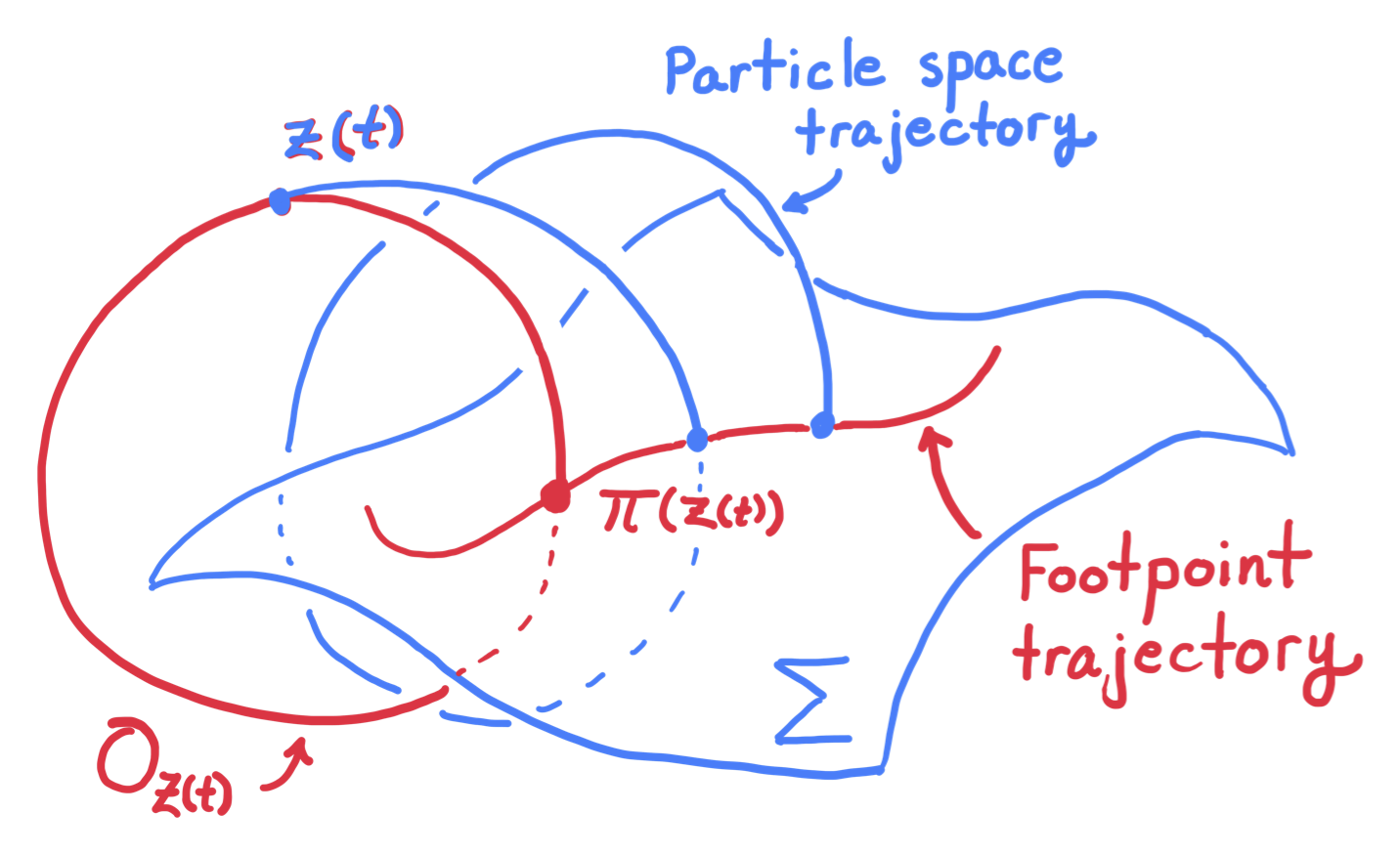
Figure 4: An illustration of Theorem 1. Although only a single $U(1)$-orbit is shown, there is such an orbit containing $z(t)$ for all times $t$.

Without further information about the ODE system $X$ finding its footpoint flow field requires detailed knowledge of the $U(1)$-orbits. These orbits are known when the underlying $U(1)$-symmetry is known in advance, but not when dealing with “hidden” symmetries, as in non-perturbative guiding center modeling. Fortunately, matters simplify considerably when $X$ is a Hamiltonian system like the Lorentz force Law. The following Theorem shows that in the Hamiltonian setting the footpoint flow field is completely determined by $\Sigma$, the Poisson bracket for $X$, the Hamiltonian for $X$, and the conserved quantity $J$ associated with the $U(1)$-action $\Phi_{\theta}$; detailed knowledge of the $U(1)$-orbits is not required.

Theorem 2.

If $X$ is a Hamiltonian system with Hamiltonian $H$ and Poisson bracket $\{\cdot,\cdot\}$ that satisfy

• $\{\cdot,\cdot\}$ and $H$ are each $U(1)$-invariant: for all $\theta\in U(1)$, $f,g:Z\rightarrow\mathbb{R}$, we have $H\circ\Phi_{\theta}=H$, $\{f\circ\Phi_{\theta},g\circ\Phi_{\theta}\}=\{f,g\}\circ\Phi_{\theta}$,

• the infinitesimal generator $R$ for the $U(1)$-action is a Hamiltonian vector field with Hamiltonian $J$,

then the following is true.

1. The hypersurface $\Sigma$ has a natural Poisson bracket $\{\cdot,\cdot\}_{\Sigma}$ with $J_{\Sigma}=J\mid\Sigma$ as a Casimir invariant. If $Z$ is equipped with coordinates $(\sigma^{i},\zeta)$, where $\zeta$ is an angular coordinate, and $\Sigma=\{\zeta=0\}$ then the $\sigma^{i}$ parameterize $\Sigma$. Moreover the Poisson bracket $\{f,g\}_{\Sigma}$ between functions $f=f(\sigma)$, and $g=g(\sigma)$ on $\Sigma$ is given explicitly by

   $$\{f,g\}_{\Sigma} =\partial_{\sigma}f^{T}\mathbb{J}_{\Sigma}\partial_{\sigma}g+\partial_{\sigma}J_{\Sigma}^{T}\mathbb{J}_{\Sigma}\,\partial_{\sigma}f\,\frac{N_{\Sigma}^{T}\partial_{\sigma}g}{N_{\Sigma}^{T}\partial_{\sigma}J_{\Sigma}}-\partial_{\sigma}J_{\Sigma}^{T}\mathbb{J}_{\Sigma}\,\partial_{\sigma}g\,\frac{N_{\Sigma}^{T}\partial_{\sigma}f}{N_{\Sigma}^{T}\partial_{\sigma}J_{\Sigma}},$$ (6)

   where the matrix $\mathbb{J}_{\Sigma}$ has components $\mathbb{J}_{\Sigma}^{ij}=\{\sigma^{i},\sigma^{j}\}(\sigma,0)$, and the column vector $N$ has components $N^{i}_{\Sigma}=\{\sigma^{i},\zeta\}(\sigma,0)$.

2. The footpoint flow field $X_{\Sigma}$ on $\Sigma$ is a Hamiltonian vector field with respect to the Poisson bracket $\{\cdot,\cdot\}_{\Sigma}$ and the Hamiltonian function $H_{\Sigma}=H\mid\Sigma$.

Proof.

Let $\{\cdot,\cdot\}$ denote the Poisson bracket on ambient phase space $Z$. If $F,G:Z\rightarrow\mathbb{R}$ are smooth functions then

$$\mathcal{L}_{R}\{F,G\}=\{\{F,G\},J\}=\{\{F,J\},G\}+\{F,\{G,J\}\}=\{\mathcal{L}_{R}F,G\}+\{F,\mathcal{L}_{R}G\},$$

because $J$ is the Hamiltonian for $R$ and $\{\cdot,\cdot\}$ satisfies the Jacobi identity. In particular, if $F,G$ are both $U(1)$-invariant, so that $\mathcal{L}_{R}F=\mathcal{L}_{R}G=0$, then so is their Poisson bracket, $\mathcal{L}_{R}\{F,G\}=0$.

Let $\iota_{\Sigma}:\Sigma\rightarrow Z$ denote the inclusion map for the Poincaré section $\Sigma$. Given smooth functions $f,g:\Sigma\rightarrow\mathbb{R}$ define their bracket according to

$$\{f,g\}_{\Sigma}=\iota_{\Sigma}^{*}\{\pi^{*}f,\pi^{*}g\},$$

where $\pi:Z\rightarrow\Sigma$ denotes the footpoint map. This bracket is clearly bilinear and skew-symmetric. It satisfies the Leibniz property because

$$\{f,gh\}_{\Sigma} =\iota_{\Sigma}^{*}\bigg{(}\{\pi^{*}f,\pi^{*}g\}\,\pi^{*}h+\{\pi^{*}f,\pi^{*}h\}\,\pi^{*}g\bigg{)}$$

$$=\{f,g\}_{\Sigma}\,\iota_{\Sigma}^{*}\pi^{*}h+\{f,h\}_{\Sigma}\,\iota_{\Sigma}^{*}\pi^{*}g$$

$$=\{f,g\}_{\Sigma}\,h+\{f,h\}_{\Sigma}\,g,$$

where we have used the Leibniz property for $\{\cdot,\cdot\}$ and $\iota_{\Sigma}^{*}\pi^{*}=(\pi\circ\iota_{\Sigma})^{*}=\text{id}_{\Sigma}^{*}=1$. It satisfies the Jacobi identity because (a) $\{\pi^{*}f,\pi^{*}g\}$ is $U(1)$-invariant since both $\pi^{*}f$ and $\pi^{*}g$ are $U(1)$-invariant, (b) $\pi^{*}\iota_{\Sigma}^{*}\{\pi^{*}f,\pi^{*}g\}=\{\pi^{*}f,\pi^{*}g\}$ since $\iota_{\Sigma}\circ\pi$ shifts points along $U(1)$-orbits, and (c) the Jacobi identity involves a cyclic sum of terms like

$$\{\{f,g\}_{\Sigma},h\}_{\Sigma} =\iota_{\Sigma}^{*}\{\pi^{*}\iota_{\Sigma}^{*}\{\pi^{*}f,\pi^{*}g\},\pi^{*}h\}=\iota_{\Sigma}^{*}\{\{\pi^{*}f,\pi^{*}g\},\pi^{*}h\},$$

which must vanish by the Jacobi identity for $\{\cdot,\cdot\}$. Thus, $\{\cdot,\cdot\}_{\Sigma}$ defines a Poisson bracket on $\Sigma$. The restriction of $J$ to $\Sigma$, $J_{\Sigma}=J\mid\Sigma=\iota_{\Sigma}^{*}J$, is a Casimir for $\{\cdot,\cdot\}_{\Sigma}$ because

$$\{f,J_{\Sigma}\}_{\Sigma}=\iota_{\Sigma}^{*}\{\pi^{*}f,\pi^{*}J_{\Sigma}\}=\iota_{\Sigma}^{*}\{\pi^{*}f,J\}=\iota_{\Sigma}^{*}(\mathcal{L}_{R}\pi^{*}f)=0,$$

for each smooth function $f$ on $\Sigma$.

The footpoint map $\pi:Z\rightarrow\Sigma$ is a Poisson map between $(Z,\{\cdot,\cdot\})$ and $(\Sigma,\{\cdot,\cdot\}_{\Sigma})$ because

$$\pi^{*}\{f,g\}_{\Sigma}=\pi^{*}\iota_{\Sigma}^{*}\{\pi^{*}f,\pi^{*}g\}=\{\pi^{*}f,\pi^{*}g\}.$$

The Hamiltonian $H$ is $U(1)$-invariant by hypothesis and therefore determined by its values on the Poincaré section, i.e. by the restriction $H_{\Sigma}=H\mid\Sigma$, in the sense that $\pi^{*}H_{\Sigma}=H$. It now follows from Guillemin-Sternberg collectivization Guillemin_Sternberg_1980 that if $z(t)$ is any solution of Hamilton’s equations on $Z$ with Hamiltonian $H=\pi^{*}H_{\Sigma}$ then the corresponding footpoint trajectory $\sigma(t)=\pi(z(t))$ is a solution of Hamilton’s equations on $\Sigma$ with Hamiltonian $H_{\Sigma}$. In other words, the footpoint trajectories are streamlines for the Hamiltonian vector field on $\Sigma$ with Hamiltonian $H_{\Sigma}$. But, by Theorem 1, the only vector field on $\Sigma$ that has footpoint trajectories as streamlines is the footpoint flow field $X_{\Sigma}$. This establishes the second part of the theorem.

To complete the proof, we must now confirm the formula (6) for the Poisson bracket $\{\cdot,\cdot\}_{\Sigma}$ in the coordinates $(\sigma^{i},\zeta)$. Without loss of generality, suppose the index $i$ takes values in $\{1,\dots,d\}$, for some integer $d$. There must be a skew-symmetric matrix $\mathbb{J}^{ij}(\sigma,\zeta)$ and a column vector $N^{i}(\sigma,\zeta)$ such that

$$\{F,G\} =\begin{pmatrix}\partial_{\sigma^{1}}F&\dots&\partial_{\sigma^{d}}F&\partial_{\zeta}F\end{pmatrix}\begin{pmatrix}\mathbb{J}&N\\ -N^{T}&0\end{pmatrix}\begin{pmatrix}\partial_{\sigma^{1}}G\\ \vdots\\ \partial_{\sigma^{d}}G\\ \partial_{\zeta}G\end{pmatrix}$$

$$=\partial_{\sigma}F^{T}\mathbb{J}\partial_{\sigma}G+\partial_{\zeta}G\,N^{T}\partial_{\sigma}F-\partial_{\zeta}F\,N^{T}\partial_{\sigma}G.$$

Setting $F=\sigma^{i}$ and $G=\sigma^{j}$ shows that the components of $\mathbb{J}$ are given by

$$\mathbb{J}^{ij}=\{\sigma^{i},\sigma^{j}\},$$

while setting $F=\sigma^{i}$ and $G=\zeta$ shows that the components of $N$ are given by

$$N^{i}=\{\sigma^{i},\zeta\}.$$

The inclusion map $\iota_{\Sigma}:\Sigma\rightarrow Z$ is given by $\sigma\mapsto(\sigma,0)$ in these coordinates. The Poisson bracket $\{\cdot,\cdot\}_{\Sigma}$ is therefore given by

$$\{f,g\}_{\Sigma}=\partial_{\sigma}f^{T}\mathbb{J}_{\Sigma}\partial_{\sigma}g+\partial_{\zeta}(\pi^{*}g)(\sigma,0)\,N_{\Sigma}^{T}\partial_{\sigma}f-\partial_{\zeta}(\pi^{*}f)(\sigma,0)\,N_{\Sigma}^{T}\partial_{\sigma}g,$$ (7)

where $\mathbb{J}_{\Sigma}=\mathbb{J}(\sigma,0)$ and $N_{\Sigma}=N(\sigma,0)$. This would be an explicit formula for $\{f,g\}_{\Sigma}$ were it not for the appearance of the $\zeta$-derivatives $\partial_{\zeta}(\pi^{*}f)(\sigma,0)$ and $\partial_{\zeta}(\pi^{*}g)(\sigma,0)$. These $\zeta$-derivatives can be expressed in terms of derivatives of $f,g$ as follows. By definition of the footpoint map $\pi$, the functions $\pi^{*}f,\pi^{*}g$ are each constant along $U(1)$-orbits. Equivalently, $\mathcal{L}_{R}\pi^{*}f=\mathcal{L}_{R}\pi^{*}g=0$. Writing the infinitesimal generator in components as $R=R^{\zeta}\,\partial_{\zeta}+\bm{R}^{i}\,\partial_{\sigma^{i}}$ therefore implies $R^{\zeta}\,\partial_{\zeta}(\pi^{*}f)+\bm{R}^{T}\,\partial_{\sigma}(\pi^{*}f)=0$, or

$$\partial_{\zeta}(\pi^{*}f)=-\frac{\bm{R}^{T}\,\partial_{\sigma}(\pi^{*}f)}{R^{\zeta}},\quad\partial_{\zeta}(\pi^{*}g)=-\frac{\bm{R}^{T}\,\partial_{\sigma}(\pi^{*}g)}{R^{\zeta}}.$$

These expressions can be simplified further using the fact that $J$ is the Hamiltonian for $R$. In particular, the components of $R$ must be given in terms of derivatives of $J$ according to

$$R^{\zeta}=\{\zeta,J\}=-N^{T}\partial_{\sigma}J,\quad\bm{R}=\{\sigma,J\}=\mathbb{J}\partial_{\sigma}J+N\,\partial_{\zeta}J.$$

The $\zeta$-derivatives are therefore

$$\partial_{\zeta}(\pi^{*}f)=\frac{(\mathbb{J}\partial_{\sigma}J+N\,\partial_{\zeta}J)^{T}\,\partial_{\sigma}(\pi^{*}f)}{N^{T}\partial_{\sigma}J},\quad\partial_{\zeta}(\pi^{*}g)=\frac{(\mathbb{J}\partial_{\sigma}J+N\,\partial_{\zeta}J)^{T}\,\partial_{\sigma}(\pi^{*}g)}{N^{T}\partial_{\sigma}J},$$

and the Poisson bracket (7) becomes

$$\{f,g\}_{\Sigma} =\partial_{\sigma}f^{T}\mathbb{J}_{\Sigma}\partial_{\sigma}g$$

$$+\frac{(\mathbb{J}_{\Sigma}\partial_{\sigma}J_{\Sigma}+N_{\Sigma}\,\partial_{\zeta}J(\sigma,0))^{T}\,\partial_{\sigma}g}{N_{\Sigma}^{T}\partial_{\sigma}J_{\Sigma}}\,N_{\Sigma}^{T}\partial_{\sigma}f$$

$$-\frac{(\mathbb{J}_{\Sigma}\partial_{\sigma}J_{\Sigma}+N_{\Sigma}\,\partial_{\zeta}J(\sigma,0))^{T}\,\partial_{\sigma}f}{N_{\Sigma}^{T}\partial_{\sigma}J_{\Sigma}}\,N_{\Sigma}^{T}\partial_{\sigma}g$$

$$=\partial_{\sigma}f^{T}\mathbb{J}_{\Sigma}\partial_{\sigma}g+\frac{(\mathbb{J}_{\Sigma}\partial_{\sigma}J_{\Sigma})^{T}\,\partial_{\sigma}g}{N_{\Sigma}^{T}\partial_{\sigma}J_{\Sigma}}\,N_{\Sigma}^{T}\partial_{\sigma}f-\frac{(\mathbb{J}_{\Sigma}\partial_{\sigma}J_{\Sigma})^{T}\,\partial_{\sigma}f}{N_{\Sigma}^{T}\partial_{\sigma}J_{\Sigma}}\,N_{\Sigma}^{T}\partial_{\sigma}g$$

$$=\partial_{\sigma}f^{T}\mathbb{J}_{\Sigma}\partial_{\sigma}g+\partial_{\sigma}J_{\Sigma}^{T}\mathbb{J}_{\Sigma}\,\partial_{\sigma}f\,\frac{N_{\Sigma}^{T}\partial_{\sigma}g}{N_{\Sigma}^{T}\partial_{\sigma}J_{\Sigma}}-\partial_{\sigma}J_{\Sigma}^{T}\mathbb{J}_{\Sigma}\,\partial_{\sigma}g\,\frac{N_{\Sigma}^{T}\partial_{\sigma}f}{N_{\Sigma}^{T}\partial_{\sigma}J_{\Sigma}}.$$

∎

Remark 3.

For the purposes of non-perturbative guiding center modeling, $\Sigma$; the Poisson bracket for $X$; and the Hamiltonian for $X$; are each known explicitly in advance. Theorem 2 therefore implies that the conserved quantity $\mathcal{J}$ associated with the “hidden” $U(1)$-symmetry of the Lorentz force Law is all that is needed to find an explicit formula for the footpoint flow field, and therefore the non-perturbatibe guiding center model. The underlying mechanism that enables this remarkable simplification is Noether’s theorem. Finding a formula for the footpoint flow field in general requires detailed knowledge of the underlying $U(1)$-symmetry. On the other hand, Noether’s theorem implies that any Hamiltonian $U(1)$-symmetry is completely determined by its corresponding conservation law. Thus, in the Hamiltonian setting complete knowledge of the Noether conserved quantity implies complete knowledge of the corresponding $U(1)$-symmetry and therefore complete knowledge of the footpoint flow field.

When Theorem 2 is applied to the Lorentz force Law written in dimensionless variables as $\dot{\bm{v}}=\bm{v}\times\bm{B}(\bm{x})$, $\dot{\bm{x}}=\epsilon\,\bm{v}$ it leads to the following characterization of the non-perturbative guiding center equations of motion in general non-vanishing magnetic fields. This result shows explicitly how to remove the assumption $\bm{B}=B(x,y)\,\bm{e}_{z}$ used in the main text. It also recovers the main text’s non-perturbative guiding center equations of motion when $\bm{B}$ is translation-invariant along $z$.

Theorem 3.

Parameterize the guiding center Poincaré section $\Sigma$ using coordinates $\bm{\mathsf{X}}=\bm{x}$, $u=v_{\parallel}$, $r=v_{\perp}$. Let $J_{\Sigma}$ denote the restriction of the non-perturbative action integral to $\Sigma$. The footpoint flow field $X_{\Sigma}=\dot{\bm{\mathsf{X}}}\cdot\partial_{\bm{\mathsf{X}}}+\dot{u}\,\partial_{u}+\dot{r}\,\partial_{r}$ on $\Sigma$ for the Lorentz force system is given explicitly by

$$D_{\epsilon}\,\dot{\bm{\mathsf{X}}}\cdot\bm{b} =\epsilon\,D_{\epsilon}\,u-{\epsilon\,\partial_{u}J_{\Sigma}\bigg{(}|\bm{B}|+\epsilon\,{(u\,\bm{b}+r\,\bm{e}_{1})\cdot[u\,r^{-1}\,\nabla\bm{b}\cdot\bm{e}_{2}+\nabla\bm{e}_{1}\cdot\bm{e}_{2}]}\bigg{)}}$$ (8)

$$D_{\epsilon}\,\dot{\bm{\mathsf{X}}}\cdot\bm{e}_{1} =\epsilon\,D_{\epsilon}\,r-\epsilon\,{\partial_{r}J_{\Sigma}\bigg{(}|\bm{B}|+\epsilon\,{(u\,\bm{b}+r\,\bm{e}_{1})\cdot[u\,r^{-1\,}\nabla\bm{b}\cdot\bm{e}_{2}+\nabla\bm{e}_{1}\cdot\bm{e}_{2}]}\bigg{)}}$$ (9)

$$D_{\epsilon}\,\dot{\bm{\mathsf{X}}}\cdot\bm{e}_{2} =-\epsilon^{2}\,{r^{-1}(u\,\bm{b}+r\,\bm{e}_{1})\cdot\partial_{\bm{\mathsf{X}}}J_{\Sigma}+\epsilon^{2}\,r^{-1}(u\,\bm{b}+r\,\bm{e}_{1})\cdot(\nabla\bm{b}\cdot\bm{e}_{1})(r\,\partial_{u}J_{\Sigma}-u\,\partial_{r}J_{\Sigma})}$$ (10)

$$D_{\epsilon}\,\dot{u} =\epsilon\,\bigg{(}\bm{B}+\epsilon\,(\bm{b}\cdot\nabla\times\bm{b})[u\,\bm{b}+r\,\bm{e}_{1}]$$

$$\hskip 30.00005pt+\epsilon\,\bm{b}\times([u\,\bm{b}+r\,\bm{e}_{1}]\cdot\nabla\bm{b})-\epsilon\,r\,\bm{e}_{2}\times(\nabla\bm{e}_{1}\cdot\bm{e}_{2})\bigg{)}\cdot\partial_{\bm{\mathsf{X}}}J_{\Sigma}$$ (11)

$$D_{\epsilon}\,\dot{r} =-\epsilon\,u\,r^{-1}\,\bigg{(}\bm{B}+\epsilon\,(\bm{b}\cdot\nabla\times\bm{b})[u\,\bm{b}+r\,\bm{e}_{1}]$$

$$\hskip 60.00009pt+\epsilon\,\bm{b}\times([u\,\bm{b}+r\,\bm{e}_{1}]\cdot\nabla\bm{b})-\epsilon\,r\,\bm{e}_{2}\times(\nabla\bm{e}_{1}\cdot\bm{e}_{2})\bigg{)}\cdot\partial_{\bm{\mathsf{X}}}J_{\Sigma},$$ (12)

where the denominator $D$ is given by

$$D_{\epsilon} =\epsilon\,r^{-1}\bm{e}_{2}\cdot\partial_{\bm{\mathsf{X}}}J_{\Sigma}+\epsilon\,r^{-1}([u\,\bm{b}+r\,\bm{e}_{1}]\cdot\nabla\bm{b}\cdot\bm{e}_{1})\,\partial_{u}J_{\Sigma}+r^{-1}|\bm{B}|\partial_{r}J_{\Sigma}$$

$$+\epsilon\,r^{-1}\,(\bm{b}\cdot\nabla\times\bm{b})(u\partial_{r}J_{\Sigma}-r\partial_{u}J_{\Sigma})+\epsilon\,(\partial_{u}J_{\Sigma}\,\bm{b}+\partial_{r}J_{\Sigma}\,\bm{e}_{1})\cdot(\nabla\bm{e}_{1}\cdot\bm{e}_{2}).$$ (13)

Proof.

We will perform the calculation for the system $\dot{\bm{v}}=\bm{v}\times\bm{B}$, $\dot{\bm{x}}=\bm{v}$. The result in the Theorem statement follows from this calculation after applying the substitutions $t\rightarrow t/\epsilon$ and $\bm{B}\rightarrow\bm{B}/\epsilon$.

In coordinate-independent form, the Poisson bracket $\{\cdot,\cdot\}$ for the Lorentz force is given by

$$\{F,G\}=\partial_{\bm{x}}F\cdot\partial_{\bm{v}}G-\partial_{\bm{x}}G\cdot\partial_{\bm{v}}F+\bm{B}\cdot\partial_{\bm{v}}F\times\partial_{\bm{v}}G.$$

In terms of the coordinates $(\bm{x},v_{\parallel},v_{\perp},\zeta)$ defined by $\bm{v}=v_{\parallel}\bm{b}+v_{\perp}(\cos\zeta\,\bm{e}_{1}+\sin\zeta\,\bm{e}_{2})$, the bracket is instead

$$\{F,G\} =\bm{b}\cdot(\partial_{\bm{x}}F\,\partial_{v_{\parallel}}G-\partial_{\bm{x}}G\,\partial_{v_{\parallel}}F)+\bm{a}\cdot(\partial_{\bm{x}}F\,\partial_{v_{\perp}}G-\partial_{\bm{x}}G\,\partial_{v_{\perp}}F)$$

$$+(v_{\perp}\,\bm{a}\cdot\nabla\bm{b}\cdot\bm{a}+v_{\parallel}\,\bm{b}\cdot\nabla\bm{b}\cdot\bm{a})(\partial_{v_{\parallel}}F\,\partial_{v_{\perp}}G-\partial_{v_{\parallel}}G\,\partial_{v_{\perp}}F)$$

$$+\bigg{(}N^{\bm{x}}\cdot\partial_{\bm{x}}F+N^{v_{\parallel}}\,\partial_{v_{\parallel}}F+N^{v_{\perp}}\,\partial_{v_{\perp}}F\bigg{)}\,\partial_{\zeta}G$$

$$-\bigg{(}N^{\bm{x}}\cdot\partial_{\bm{x}}G+N^{v_{\parallel}}\,\partial_{v_{\parallel}}G+N^{v_{\perp}}\,\partial_{v_{\perp}}G\bigg{)}\,\partial_{\zeta}F,$$

where $\bm{a}=\cos\zeta\,\bm{e}_{1}+\sin\zeta\,\bm{e}_{2}$, $\bm{c}=\bm{a}\times\bm{b}=-\cos\zeta\,\bm{e}_{2}+\sin\zeta\,\bm{e}_{1}$, and the components of $N$ are given by

$$N^{\bm{x}} =-\frac{1}{v_{\perp}}\bm{c}$$ (14)

$$N^{v_{\parallel}} =-\bm{c}\cdot\nabla\bm{b}\cdot\bm{a}-\frac{v_{\parallel}}{v_{\perp}}(\bm{b}\cdot\nabla\bm{b})\cdot\bm{c}+\bm{b}\cdot\nabla\bm{e}_{1}\cdot\bm{e}_{2}$$ (15)

$$N^{v_{\perp}} =\frac{|\bm{B}|}{v_{\perp}}+\frac{v_{\parallel}}{v_{\perp}}\,\bm{b}\cdot\nabla\times\bm{b}+\bm{a}\cdot\nabla\bm{e}_{1}\cdot\bm{e}_{2}.$$ (16)

Theorem 2 therefore implies that the Poisson bracket $\{\cdot,\cdot\}_{\Sigma}$ on the guiding center Poincaré section is given by,

$$\{f,g\}_{\Sigma} =\bm{b}\cdot(\partial_{\bm{\mathsf{X}}}f\,\partial_{u}g-\partial_{\bm{\mathsf{X}}}g\,\partial_{u}f)+\bm{e}_{1}\cdot(\partial_{\bm{\mathsf{X}}}f\,\partial_{r}g-\partial_{\bm{\mathsf{X}}}g\,\partial_{r}f)$$

$$+(r\,\bm{e}_{1}\cdot\nabla\bm{b}\cdot\bm{e}_{1}+u\,\bm{b}\cdot\nabla\bm{b}\cdot\bm{e}_{1})(\partial_{u}f\,\partial_{r}g-\partial_{u}g\,\partial_{r}f)$$

$$+\bigg{(}\bm{b}\cdot(\partial_{\bm{\mathsf{X}}}J_{\Sigma}\,\partial_{u}f-\partial_{\bm{\mathsf{X}}}f\,\partial_{u}J_{\Sigma})+\bm{e}_{1}\cdot(\partial_{\bm{\mathsf{X}}}J_{\Sigma}\,\partial_{r}f-\partial_{\bm{\mathsf{X}}}f\,\partial_{r}J_{\Sigma})$$

$$+(r\,\bm{e}_{1}\cdot\nabla\bm{b}\cdot\bm{e}_{1}+u\,\bm{b}\cdot\nabla\bm{b}\cdot\bm{e}_{1})(\partial_{u}J_{\Sigma}\,\partial_{r}f-\partial_{u}f\,\partial_{r}J_{\Sigma})\bigg{)}\frac{N^{\bm{\mathsf{X}}}_{\Sigma}\cdot\partial_{\bm{\mathsf{X}}}g+N^{u}_{\Sigma}\,\partial_{u}g+N^{r}_{\Sigma}\,\partial_{r}g}{N^{\bm{\mathsf{X}}}_{\Sigma}\cdot\partial_{\bm{\mathsf{X}}}J_{\Sigma}+N^{u}_{\Sigma}\,\partial_{u}J_{\Sigma}+N^{r}_{\Sigma}\,\partial_{r}J_{\Sigma}}$$

$$-\bigg{(}\bm{b}\cdot(\partial_{\bm{\mathsf{X}}}J_{\Sigma}\,\partial_{u}g-\partial_{\bm{\mathsf{X}}}g\,\partial_{u}J_{\Sigma})+\bm{e}_{1}\cdot(\partial_{\bm{\mathsf{X}}}J_{\Sigma}\,\partial_{r}g-\partial_{\bm{\mathsf{X}}}g\,\partial_{r}J_{\Sigma})$$

$$+(r\,\bm{e}_{1}\cdot\nabla\bm{b}\cdot\bm{e}_{1}+u\,\bm{b}\cdot\nabla\bm{b}\cdot\bm{e}_{1})(\partial_{u}J_{\Sigma}\,\partial_{r}g-\partial_{u}g\,\partial_{r}J_{\Sigma})\bigg{)}\frac{N^{\bm{\mathsf{X}}}_{\Sigma}\cdot\partial_{\bm{\mathsf{X}}}f+N^{u}_{\Sigma}\,\partial_{u}f+N^{r}_{\Sigma}\,\partial_{r}f}{N^{\bm{\mathsf{X}}}_{\Sigma}\cdot\partial_{\bm{\mathsf{X}}}J_{\Sigma}+N^{u}_{\Sigma}\,\partial_{u}J_{\Sigma}+N^{r}_{\Sigma}\,\partial_{r}J_{\Sigma}},$$

where

$$N^{\bm{\mathsf{X}}}_{\Sigma} =r^{-1}\bm{e}_{2}$$

$$N^{u}_{\Sigma} =r^{-1}(u\bm{b}+r\bm{e}_{1})\cdot\nabla\bm{b}\cdot\bm{e}_{2}-\bm{b}\cdot\nabla\times\bm{b}+\bm{b}\cdot\nabla\bm{e}_{1}\cdot\bm{e}_{2}$$

$$N^{r}_{\Sigma} =r^{-1}|\bm{B}|+r^{-1}u\,\bm{b}\cdot\nabla\times\bm{b}+\bm{e}_{1}\cdot\nabla\bm{e}_{1}\cdot\bm{e}_{2}.$$

By Theorem 2, the footpoint flow field for the Lorentz force is given by Hamilton’s equations $\dot{\sigma}^{i}=\{\sigma^{i},H_{\Sigma}\}_{\Sigma}$. The above explicit expression for $\{\cdot,\cdot\}_{\Sigma}$, together with $H_{\Sigma}=\frac{1}{2}u^{2}+\frac{1}{2}r^{2}$, therefore implies the following explicit expressions for the components of the footpoint flow field. The $\bm{X}$-component is

$$\{\bm{\mathsf{X}},H_{\Sigma}\}_{\Sigma} =u\,\bm{b}+r\,\bm{e}_{1}$$

$$+\bigg{(}-\partial_{u}J_{\Sigma}\,\bm{b}-\partial_{r}J_{\Sigma}\,\bm{e}_{1}\bigg{)}\frac{N^{u}_{\Sigma}\,u+N^{r}_{\Sigma}\,r}{N^{\bm{\mathsf{X}}}_{\Sigma}\cdot\partial_{\bm{\mathsf{X}}}J_{\Sigma}+N^{u}_{\Sigma}\,\partial_{u}J_{\Sigma}+N^{r}_{\Sigma}\,\partial_{r}J_{\Sigma}}$$

$$-\bigg{(}(u\,\bm{b}+r\,\bm{e}_{1})\cdot\partial_{\bm{\mathsf{X}}}J_{\Sigma}$$

$$+(r\,\bm{e}_{1}\cdot\nabla\bm{b}\cdot\bm{e}_{1}+u\,\bm{b}\cdot\nabla\bm{b}\cdot\bm{e}_{1})(\partial_{u}J_{\Sigma}\,r-u\,\partial_{r}J_{\Sigma})\bigg{)}\frac{N^{\bm{\mathsf{X}}}_{\Sigma}}{N^{\bm{\mathsf{X}}}_{\Sigma}\cdot\partial_{\bm{\mathsf{X}}}J_{\Sigma}+N^{u}_{\Sigma}\,\partial_{u}J_{\Sigma}+N^{r}_{\Sigma}\,\partial_{r}J_{\Sigma}},$$

$$=u\,\bm{b}+r\,\bm{e}_{1}$$

$$-\frac{(\partial_{u}J_{\Sigma}\,\bm{b}+\partial_{r}J_{\Sigma}\,\bm{e}_{1})(N^{u}_{\Sigma}\,u+N^{r}_{\Sigma}\,r)}{N^{\bm{\mathsf{X}}}_{\Sigma}\cdot\partial_{\bm{\mathsf{X}}}J_{\Sigma}+N^{u}_{\Sigma}\,\partial_{u}J_{\Sigma}+N^{r}_{\Sigma}\,\partial_{r}J_{\Sigma}}$$

$$-\frac{(u\,\bm{b}+r\,\bm{e}_{1})\cdot\partial_{\bm{\mathsf{X}}}J_{\Sigma}\,N^{\bm{\mathsf{X}}}_{\Sigma}}{N^{\bm{\mathsf{X}}}_{\Sigma}\cdot\partial_{\bm{\mathsf{X}}}J_{\Sigma}+N^{u}_{\Sigma}\,\partial_{u}J_{\Sigma}+N^{r}_{\Sigma}\,\partial_{r}J_{\Sigma}}$$

$$-\frac{(r\,\bm{e}_{1}\cdot\nabla\bm{b}\cdot\bm{e}_{1}+u\,\bm{b}\cdot\nabla\bm{b}\cdot\bm{e}_{1})(\partial_{u}J_{\Sigma}\,r-u\,\partial_{r}J_{\Sigma})N^{\bm{\mathsf{X}}}_{\Sigma}}{N^{\bm{\mathsf{X}}}_{\Sigma}\cdot\partial_{\bm{\mathsf{X}}}J_{\Sigma}+N^{u}_{\Sigma}\,\partial_{u}J_{\Sigma}+N^{r}_{\Sigma}\,\partial_{r}J_{\Sigma}}$$

$$=u\,\bm{b}+r\,\bm{e}_{1}$$

$$-\frac{\partial_{u}J_{\Sigma}(uN^{u}_{\Sigma}+r\,N^{r}_{\Sigma})}{N^{\bm{\mathsf{X}}}_{\Sigma}\cdot\partial_{\bm{\mathsf{X}}}J_{\Sigma}+N^{u}_{\Sigma}\,\partial_{u}J_{\Sigma}+N^{r}_{\Sigma}\,\partial_{r}J_{\Sigma}}\,\bm{b}$$

$$-\frac{\partial_{r}J_{\Sigma}(uN^{u}_{\Sigma}+r\,N^{r}_{\Sigma})}{N^{\bm{\mathsf{X}}}_{\Sigma}\cdot\partial_{\bm{\mathsf{X}}}J_{\Sigma}+N^{u}_{\Sigma}\,\partial_{u}J_{\Sigma}+N^{r}_{\Sigma}\,\partial_{r}J_{\Sigma}}\,\bm{e}_{1}$$

$$-\frac{(\frac{u}{r}\bm{b}+\bm{e}_{1})\cdot\partial_{\bm{\mathsf{X}}}J_{\Sigma}+(\bm{e}_{1}\cdot\nabla\bm{b}\cdot\bm{e}_{1}+\frac{u}{r}\,\bm{b}\cdot\nabla\bm{b}\cdot\bm{e}_{1})(r\,\partial_{u}J_{\Sigma}-u\,\partial_{r}J_{\Sigma})}{N^{\bm{\mathsf{X}}}_{\Sigma}\cdot\partial_{\bm{\mathsf{X}}}J_{\Sigma}+N^{u}_{\Sigma}\,\partial_{u}J_{\Sigma}+N^{r}_{\Sigma}\,\partial_{r}J_{\Sigma}}\,\bm{e}_{2}$$

$$=u\,\bm{b}+r\,\bm{e}_{1}$$

$$-\frac{\partial_{u}J_{\Sigma}(|\bm{B}|+u\,\bm{b}\cdot\nabla\times\bm{b}+u\,\bm{e}_{2}\cdot\nabla\bm{b}\cdot\bm{e}_{1}+\frac{u^{2}}{r}\bm{b}\cdot\nabla\bm{b}\cdot\bm{e}_{2}+(u\bm{b}+r\,\bm{e}_{1})\cdot\nabla\bm{e}_{1}\cdot\bm{e}_{2})}{N^{\bm{\mathsf{X}}}_{\Sigma}\cdot\partial_{\bm{\mathsf{X}}}J_{\Sigma}+N^{u}_{\Sigma}\,\partial_{u}J_{\Sigma}+N^{r}_{\Sigma}\,\partial_{r}J_{\Sigma}}\,\bm{b}$$

$$-\frac{\partial_{r}J_{\Sigma}(|\bm{B}|+u\,\bm{b}\cdot\nabla\times\bm{b}+u\,\bm{e}_{2}\cdot\nabla\bm{b}\cdot\bm{e}_{1}+\frac{u^{2}}{r}\bm{b}\cdot\nabla\bm{b}\cdot\bm{e}_{2}+(u\bm{b}+r\,\bm{e}_{1})\cdot\nabla\bm{e}_{1}\cdot\bm{e}_{2})}{N^{\bm{\mathsf{X}}}_{\Sigma}\cdot\partial_{\bm{\mathsf{X}}}J_{\Sigma}+N^{u}_{\Sigma}\,\partial_{u}J_{\Sigma}+N^{r}_{\Sigma}\,\partial_{r}J_{\Sigma}}\,\bm{e}_{1}$$

$$-\frac{(\frac{u}{r}\bm{b}+\bm{e}_{1})\cdot\partial_{\bm{\mathsf{X}}}J_{\Sigma}+(\bm{e}_{1}\cdot\nabla\bm{b}\cdot\bm{e}_{1}+\frac{u}{r}\,\bm{b}\cdot\nabla\bm{b}\cdot\bm{e}_{1})(r\,\partial_{u}J_{\Sigma}-u\,\partial_{r}J_{\Sigma})}{N^{\bm{\mathsf{X}}}_{\Sigma}\cdot\partial_{\bm{\mathsf{X}}}J_{\Sigma}+N^{u}_{\Sigma}\,\partial_{u}J_{\Sigma}+N^{r}_{\Sigma}\,\partial_{r}J_{\Sigma}}\,\bm{e}_{2},$$

which reproduces Eqs. (8)-(10) in the Theorem statement. The $u$-component is

$$\{u,H_{\Sigma}\}_{\Sigma} =$$

$$+r\,(r\,\bm{e}_{1}\cdot\nabla\bm{b}\cdot\bm{e}_{1}+u\,\bm{b}\cdot\nabla\bm{b}\cdot\bm{e}_{1})$$

$$+\bigg{(}\bm{b}\cdot\partial_{\bm{\mathsf{X}}}J_{\Sigma}-(r\,\bm{e}_{1}\cdot\nabla\bm{b}\cdot\bm{e}_{1}+u\,\bm{b}\cdot\nabla\bm{b}\cdot\bm{e}_{1})\partial_{r}J_{\Sigma}\bigg{)}\frac{N^{u}_{\Sigma}\,u+N^{r}_{\Sigma}\,r}{N^{\bm{\mathsf{X}}}_{\Sigma}\cdot\partial_{\bm{\mathsf{X}}}J_{\Sigma}+N^{u}_{\Sigma}\,\partial_{u}J_{\Sigma}+N^{r}_{\Sigma}\,\partial_{r}J_{\Sigma}}$$

$$-\bigg{(}(u\,\bm{b}+r\,\bm{e}_{1})\cdot\partial_{\bm{\mathsf{X}}}J_{\Sigma}$$

$$+(r\,\bm{e}_{1}\cdot\nabla\bm{b}\cdot\bm{e}_{1}+u\,\bm{b}\cdot\nabla\bm{b}\cdot\bm{e}_{1})(\partial_{u}J_{\Sigma}\,r-u\,\partial_{r}J_{\Sigma})\bigg{)}\frac{N^{u}_{\Sigma}}{N^{\bm{\mathsf{X}}}_{\Sigma}\cdot\partial_{\bm{\mathsf{X}}}J_{\Sigma}+N^{u}_{\Sigma}\,\partial_{u}J_{\Sigma}+N^{r}_{\Sigma}\,\partial_{r}J_{\Sigma}}$$

$$=\frac{r\,(r\bm{e}_{1}\cdot\nabla\bm{b}\cdot\bm{e}_{1}+u\bm{b}\cdot\nabla\bm{b}\cdot\bm{e}_{1})\,N^{\bm{\mathsf{X}}}_{\Sigma}\cdot\partial_{\bm{\mathsf{X}}}J_{\Sigma}}{D}$$

$$+\frac{r(N^{r}_{\Sigma}\,\bm{b}-N^{u}_{\Sigma}\,\bm{e}_{1})\cdot\partial_{\bm{\mathsf{X}}}J_{\Sigma}}{D}$$

$$=\frac{(|\bm{B}|+u\bm{b}\cdot\nabla\times\bm{b}+r\,\bm{e}_{1}\cdot\nabla\bm{e}_{1}\cdot\bm{e}_{2})}{D}\bm{b}\cdot\partial_{\bm{\mathsf{X}}}J_{\Sigma}$$

$$-\frac{(r\bm{e}_{1}\cdot\nabla\bm{b}\cdot\bm{e}_{2}-r\bm{b}\cdot\nabla\times\bm{b}+u\bm{b}\cdot\nabla\bm{b}\cdot\bm{e}_{2}+r\bm{b}\cdot\nabla\bm{e}_{1}\cdot\bm{e}_{2})}{D}\bm{e}_{1}\cdot\partial_{\bm{\mathsf{X}}}J_{\Sigma}$$

$$+\frac{(r\,\bm{e}_{1}\cdot\nabla\bm{b}\cdot\bm{e}_{1}+u\bm{b}\cdot\nabla\bm{b}\cdot\bm{e}_{1})}{D}\bm{e}_{2}\cdot\partial_{\bm{\mathsf{X}}}J_{\Sigma}$$

$$=\frac{\bm{B}+(\bm{b}\cdot\nabla\times\bm{b})[u\,\bm{b}+r\,\bm{e}_{1}]+\bm{b}\times([u\bm{b}+r\bm{e}_{1}]\cdot\nabla\bm{b})-r\,\bm{e}_{2}\times(\nabla\bm{e}_{1}\cdot\bm{e}_{2})}{D}\cdot\partial_{\bm{\mathsf{X}}}J_{\Sigma},$$

which reproduces Eq. (11). Finally, the $r$-component is

$$\{r,H_{\Sigma}\}_{\Sigma} =-u(r\,\bm{e}_{1}\cdot\nabla\bm{b}\cdot\bm{e}_{1}+u\,\bm{b}\cdot\nabla\bm{b}\cdot\bm{e}_{1})$$

$$+\bigg{(}\bm{e}_{1}\cdot(\partial_{\bm{\mathsf{X}}}J_{\Sigma})$$

$$+(r\,\bm{e}_{1}\cdot\nabla\bm{b}\cdot\bm{e}_{1}+u\,\bm{b}\cdot\nabla\bm{b}\cdot\bm{e}_{1})(\partial_{u}J_{\Sigma})\bigg{)}\frac{N^{u}_{\Sigma}\,u+N^{r}_{\Sigma}\,r}{N^{\bm{\mathsf{X}}}_{\Sigma}\cdot\partial_{\bm{\mathsf{X}}}J_{\Sigma}+N^{u}_{\Sigma}\,\partial_{u}J_{\Sigma}+N^{r}_{\Sigma}\,\partial_{r}J_{\Sigma}}$$

$$-\bigg{(}(u\,\bm{b}+r\,\bm{e}_{1})\cdot\partial_{\bm{\mathsf{X}}}J_{\Sigma}$$

$$+(r\,\bm{e}_{1}\cdot\nabla\bm{b}\cdot\bm{e}_{1}+u\,\bm{b}\cdot\nabla\bm{b}\cdot\bm{e}_{1})(\partial_{u}J_{\Sigma}\,r-u\,\partial_{r}J_{\Sigma})\bigg{)}\frac{N^{r}_{\Sigma}}{N^{\bm{\mathsf{X}}}_{\Sigma}\cdot\partial_{\bm{\mathsf{X}}}J_{\Sigma}+N^{u}_{\Sigma}\,\partial_{u}J_{\Sigma}+N^{r}_{\Sigma}\,\partial_{r}J_{\Sigma}}$$

$$=-\frac{u\,(r\,\bm{e}_{1}\cdot\nabla\bm{b}\cdot\bm{e}_{1}+u\,\bm{b}\cdot\nabla\bm{b}\cdot\bm{e}_{1})\,N^{\bm{\mathsf{X}}}_{\Sigma}}{D}\cdot\partial_{\bm{\mathsf{X}}}J_{\Sigma}$$

$$+\frac{u\,N^{u}_{\Sigma}\,\bm{e}_{1}-u\,N^{r}_{\Sigma}\,\bm{b}}{D}\cdot\partial_{\bm{\mathsf{X}}}J_{\Sigma}$$

$$=\frac{-\frac{u}{r}\bm{b}\times([u\bm{b}+r\bm{e}_{1}]\cdot\nabla\bm{b})-\frac{u}{r}[u\bm{b}+r\bm{e}_{1}](\bm{b}\cdot\nabla\times\bm{b})+u\bm{e}_{2}\times(\nabla\bm{e}_{1}\cdot\bm{e}_{2})}{D}\cdot\partial_{\bm{\mathsf{X}}}J_{\Sigma},$$

which reproduced Eq. (12) from the Theorem statement.

∎

II Low-noise derivative estimation

This Section describes the method we used to estimate “ground truth” time derivatives of (presumptive) continuous-time trajectories on $\Sigma$ that interpolate iterates of the Poincaré map. To provide good input data to estimate $\mathcal{J}$, we need to be confident that we can both trust that a point $(x,y,r)$ is integrable and that we have a good estimate of the derivative $(\dot{x},\dot{y})$. For both of these tasks, we leverage the Birkhoff Reduced Rank Extrapolation (Birkhoff RRE) algorithm Ruth:2024 implemented in the SymplecticMapTools.jl Julia package. Using a single trajectory from the Poincaré map, here denoted $F$, Birkhoff RRE first classifies that trajectory as an invariant circle, an island, or chaos. Then, assuming the trajectory is an invariant circle with Diophantine rotation number $\omega$, it returns an approximate parameterization of an invariant circle $z:\mathbb{T}\to\Sigma$ and $\omega$ so that $F(z(\theta))=z(\theta+\omega)$. Clearly, the adiabatic invariant $\mathcal{J}$ should be constant on $z$, meaning that $\dot{z}\cdot\nabla\mathcal{J}=0$, giving the correct direction of the derivatives of $\dot{z}$ in 2D.

To obtain the magnitude of of the derivatives, we first observe that the dynamics predicted by the non-perturbative guiding center equations of motion on the invariant circle will have the form $(\dot{x},\dot{y})=({dz}/{d\theta})\dot{\theta}$. To estimate $\dot{\theta}$, we note it must satisfy a differential equation of the form

$$\dot{\theta}=f(\theta),\qquad\theta(t+T(\theta(t)))=\theta(t)+\omega,$$

where $T(\theta(t))$ is the gyroperiod at the point $z(\theta(t))$. We can lift and invert the dynamics to find

$$\frac{dt}{d\theta}=g(t),\qquad t(\theta+\omega)=t(\theta)+T(\theta).$$

For Diophantine $\omega$ and smooth enough $T$, we can solve the right expression for $t$ to find

$$t(\theta)=c+t_{0}\theta+\sideset{}{{}^{\prime}}{\sum}_{n=-N}^{N}t_{n}e^{in\theta},$$

where $c$ is a constant determined by initial conditions and

$$t_{n}=\begin{cases}\frac{1}{\omega}\langle T\rangle&n=0\\ \frac{1}{e^{in\omega}-1}\langle T(\cdot)e^{-in\cdot}\rangle&n\neq 0\end{cases},\quad\langle f\rangle=\frac{1}{2\pi}\int_{\mathbb{T}}f(\theta)\,d\theta.$$

Using a discrete Fourier transform to compute the above quantities and $\dot{\theta}=({dt}/{d\theta})^{-1}$, we have an approximation of $(\dot{x},\dot{y})$.

References

[1]
A. H. Boozer.
Transport and isomorphic equilibria.
Phys. Fluids, 26:496, 1983.
[2]
J. Nürenberg and R. Zille.
Quasihelically symmetric toroidal stellarators.
Phys. Lett. A, 129:113–117, 1988.
[3]
J. W. Burby and H. Qin.
Toroidal precession as a geometric phase.
Phys. Plasmas, 20:012511, 2013.
[4]
P. Helander.
Theory of plasma confinement in non-axisymmetric magnetic fields.
Rep. Prog. Phys., 77:087001, 2014.
[5]
J. W. Burby, N. Kallinikos, and R. S. MacKay.
Some mathematics for quasisymmetry.
J. Math. Phys., 61:093503, 2020.
[6]
E. Rodriguez, P. Helander, and A. Bhattacharjee.
Necessary and sufficient conditions for quasisymmetry.
Phys. Plasmas, 27:062501, 2020.
[7]
L. S. Hall and B. McNamara.
Three-dimensional equilibrium of the anisotropic , finite-pressure guiding-center plasma: Theory of the magnetic plasma.
Phys. Fluids, 18:552–565, 1975.
[8]
M. Landreman and P. J. Catto.
Omnigeneity as generalized quasisymmetry.
Phys. Plasmas, 19:056103, 2012.
[9]
F. I. Parra, I. Calvo, P. Helander, and M. Landreman.
Less constrained omnigeneous stellarators.
Nucl. Fusion, 55:033005, 2015.
[10]
A. G. Goodman, K. Camacho Mata, S. A. Henneberg, R. Jorge, M. Landreman, G. G. Plunk, H. M. Smith, R. J. J. Mackenbach, C. D. Beidler, and P. Helander.
Constructing precisely quasi-isodynamic magnetic fields.
J. Plasma Phys., 89:905890504, 2023.
[11]
J. W. Burby, R. S. MacKay, and S. Naik.
Isodrastic magnetic fields for suppressing transitions in guiding-centre motion.
Nonlinearity, 36:5884, 2023.
[12]
M. Kruskal.
Asymptotic theory of hamiltonian and other systems with all solutions nearly periodic.
J. Math. Phys., 3:806, 1962.
[13]
R. G. Littlejohn.
Hamiltonian formulation of guiding center motion.
Phys. Fluids, 24:1730, 1981.
[14]
R. G. Littlejohn.
Variational principles of guiding centre motion.
J. Plasma Phys., 29:111, 1983.
[15]
R. G. Littlejohn.
Geometry and guiding center motion.
In J. E. Marsden, editor, Fluids and Plasmas: Geometry and Dynamics, volume 28 of Contemporary mathematics, pages 151–167. American Mathematical Society, 1984.
[16]
J. Cary and A. J. Brizard.
Hamiltonian theory of guiding-center motion.
Rev. Mod. Phys., 81:693, 2009.
[17]
J. W. Burby.
Guiding center dynamics as motion on a formal slow manifold in loop space.
J. Math. Phys., 61:012703, 2020.
[18]
J. W. Burby, J. Squire, and H. Qin.
Automation of the guiding center expansion.
Phys. Plasmas, 20:072105, 2013.
[19]
M. Berry.
Asymptotics beyond all orders, chapter Asymptotics, superasymptotics, hyperasymptotics, pages 1–14.
Plenum, Amsterdam, 1991.
[20]
V. Guillemin and A. Pollack.
Differential topology.
Prentice-Hall, 1974.
[21]
D. A. Messenger, J. W. Burby, and D. M. Bortz.
Coarse-graining hamiltonian systems using wsindy.
Sci. Rep., 14:14457, 2024.
[22]
M. Ruth and D. Bindel.
Finding Birkhoff Averages via Adaptive Filtering, 2024.
arXiv:2403.19003 [math.DS].
[23]
M. Ruth and D. Bindel.
Level Set Learning for Poincaré Plots of Symplectic Maps, 2023.
arXiv:2312.00967 [physics].
[24]
C. G. Albert, S. V. Kasilov, and W. Kernbichler.
Accelerated methods for direct computation of fusion alpha particle losses within, stellarator optimization.
J. Plasma Phys., 86(2):815860201, 2020.
[25]
C. G. Albert, R. Buchholz, S. V. Kasilov, W. Kernbichler, and K. Rath.
Alpha particle confinement metrics based on orbit classification in stellarators.
J. Plasma Phys., 89(3):955890301, 2023.
[26]
L. Lu, P. Jin, G. Pang, Z. Zhang, and G. E. Karniadakis.
Learning nonlinear operators via DeepONet based on the universal approximation theorem of operators.
Nature Mach. Intell., 3:218–229, 2021.
[27]
S. L. Brunton, J. L. Proctor, and J. N. Kutz.
Discovering governing equations from data by sparse identification of nonlinear dynamical systems.
PNAS, 113:3932–3937, 2016.
[28]
D. A. Messenger and D. M. Bortz.
Weak sindy: Galerkin-based data-driven model selection.
Multiscale Model. Simul., 19:1474–1497, 2021.
[29]
V. Guillemin and S. Sternberg.
The moment map and collective motion.
Ann. Phys., 127:220–253, 1980.