Quantum Mutual Information in Time
Abstract
While the quantum mutual information is a fundamental measure of quantum information, it is only defined for spacelike-separated quantum systems. Such a limitation is not present in the theory of classical information, where the mutual information between two random variables is well-defined irrespective of whether or not the variables are separated in space or separated in time. Motivated by this disparity between the classical and quantum mutual information, we employ the pseudo-density matrix formalism to define a simple extension of quantum mutual information into the time domain. As in the spatial case, we show that such a notion of quantum mutual information in time serves as a natural measure of correlation between timelike-separated systems, while also highlighting ways in which quantum correlations distinguish between space and time. We also show how such quantum mutual information is time-symmetric with respect to quantum Bayesian inversion, and then we conclude by showing how mutual information in time yields a Holevo bound for the amount of classical information that may be extracted from sequential measurements on an ensemble of quantum states.
I Introduction
The mutual information of two quantum systems and whose joint state is represented by a bipartite density matrix is the real number given by
| (1) |
where denotes the von Neumann entropy and and are the reduced density matrices of Cerf and Adami (1997); Nielsen and Chuang (2011). As describes the joint state of two spacelike separated systems and , it follows that the quantum mutual information is essentially a static measure of information. This non-dynamical nature of quantum mutual information is in stark contrast with the notion of the classical mutual information of two random variables and , which is defined irrespective of whether and are separated in space or in time Cover and Thomas (2006).
In this work, we make use of the pseudo-density matrix (PDM) formalism Fitzsimons et al. (2015); Fullwood and Parzygnat (2024) to define a temporal extension of quantum mutual information, and we investigate its properties. A PDM is a generalization of a density matrix that encodes correlations across both space and time, thus providing a single mathematical formalism for the study of both static and dynamical aspects of quantum information (see Refs. Marletto et al. (2021); Zhao et al. (2018); Pisarczyk et al. (2019); Marletto et al. (2020, 2019); Liu et al. (2024, 2023); Fullwood and Parzygnat (2024); Song et al. (2024); Jia et al. (2023); Parzygnat and Fullwood (2024) for further development and applications of PDMs). In particular, PDMs provide a notion of a joint state associated with timelike separated quantum systems and whose reduced density matrices are the individual states and . However, while is Hermitian and of unit trace, it is not positive in general. Thus, the extension of the density matrix formalism to include non-positive PDMs is akin to the way in which the metric of space is extended into the time domain in special relativity, where such an extension results in a metric of Lorentzian (as opposed to Euclidean) signature French (1968); Hawking and Ellis (1973).
As for defining quantum mutual information in time, note that since the logarithm is not uniquely defined for non-positive matrices, simply replacing by in equation (1) will not in general yield a well-defined notion of quantum mutual information in time. To circumvent this issue, we use an extension of von Neumann entropy to Hermitian matrices given by Fullwood and Parzygnat (2023); Parzygnat et al. (2023); Tu et al. (2022); Salek et al. (2014)
| (2) |
While there are various justifications for our choice of over other alternatives (such as those used e.g. in Refs. Jia et al. (2023); Parzygnat et al. (2023)), a primary justification is that satisfies Fullwood and Parzygnat (2023)
-
•
(Additivity) for all Hermitian matrices and .
-
•
(Orthogonal Convexity) If is a collection of mutually orthogonal Hermitian matrices of unit trace and is a probability distribution, then
where is the Shannon entropy of the probability distribution .
While the properties of additivity and orthogonal convexity are certainly desirable from a purely mathematical perspective, we show in Section VI that additivity and orthogonal convexity of are also crucial for establishing a temporal analog of the Holevo bound Holevo (1973), thus providing an operational justification for the use of .
Employing such a Hermitian extension of von Neumann entropy and replacing by a pseudo-density matrix in equation (1) yields a well-defined notion of quantum mutual information for timelike separated quantum systems. In what follows, we prove general statements regarding such a notion of mutual information in time and present many examples. As in the spatial case, we find that such a mutual information in time provides a natural measure of correlation between timelike separated systems, while also highlighting the way in which quantum correlations distinguish between space and time. In particular, for sequential measurements performed on a system of qubits at two times, we show in Section III that the mutual information vanishes for a system which is discarded and re-prepared between measurements, while it is maximized for a system undergoing unitary evolution between measurements. However, contrary to spatial mutual information, which for a pair of spacelike separated qubits can attain a maximum value of 2 in the presence of entanglement, we show in Section IV that the mutual information in time between two timelike separated qubits never exceeds a value of 1. We argue that this is a reflection of the fact that, unlike spatial correlations, maximal correlations in time are non-monogamous Marletto et al. (2020), as a qubit at a fixed point in time may be maximally correlated with a qubit both at a time in the future and a time in the past.
While for mutual information in space it is manifest from definition (1) that , for mutual information in time the existence of such a symmetry is more subtle, as systems and may be related in time by a non-reversible process. However, we show in Section V that when the quantum channel establishing temporal correlations between and is Bayesian invertible in the sense defined in Ref. Parzygnat and Fullwood (2023), then it is fact that case that , in accordance with the spatial case.
II Pseudo-density matrices
Let denote the th Pauli matrix for , and let be a positive integer. For every , we let denote the th component of for all , and then define as
Suppose a sequential measurement of followed by is performed on a system of -qubits at times and with , and denote the Hilbert spaces of the system at the two times by and , respectively. If the system evolves according to the quantum channel between measurements (we use to denote the algebra of linear operators on a Hilbert space ), then the theoretical two-time expectation value of the sequential measurement of followed by is the real number given by
where is the initial state of the system, and is the orthogonal projection operator onto the -eigenspace of .
In such a two-time measurement scenario, the associated pseudo-density matrix (PDM) is defined to be the bipartite hermitian operator on given by
| (3) |
It follows from the definition of PDM together with properties of Pauli matrices that for all and ,
| (4) |
Thus, PDMs extend the operational meaning of bipartite density matrices to the temporal domain for Pauli observables.
Although the definition of PDM is conceptually simple, it is not always practical for calculations. In Refs. Horsman et al. (2017); Liu et al. (2023); Fullwood and Parzygnat (2024), it was shown that the PDM defined by (3) may be given by the formula
| (5) |
where denotes the anticommutator and is the Jamiołkowski matrix of the channel Jamiołkowski (1972). When we wish to emphasize the dependence of the PDM on the initial state and channel as part of a two-time measurement scenario, we denote the RHS of Eq. (5) by and refer to it as the spatiotemporal product of the channel and the initial state .
The notion of PDM naturally extends to -sequential measurements on a system of -qubits for arbitrary , yielding an operator on the -fold tensor product , where denotes the system at time , with . We denote such an -time PDM simply by . If the system evolves according to a channel between measurements at times and for , it was shown in Refs. Liu et al. (2023); Fullwood (2023a) that may be given by the recursive formula
| (6) |
where is the partial trace over the subsystems and denotes the spatiotemporal product.
We note that while PDMs are not positive in general, they are always Hermitian and of unit trace. Moreover, the reduced marginals onto a single factor are always density matrices, representing the state of the system at time . Interestingly, positive PDMs admit dual interpretations as being extended across space on the one hand, and time on the other. We refer to such PDMs as dual states.
III Mutual Information in Time
Let be an -time PDM as in (6), let denote the associated system at time for , let , and let and be the PDMs corresponding to the first measurements and final measurements, respectively, which may be obtained from the PDM by tracing out the associated complementary subsystems. We then define the mutual information in time between the joint temporal systems and to be the element given by
where is the Hermitian extension of the von Neumann entropy given by .
We now present some examples of mutual information in time.
Example 1 (A dual state).
Let be the bipartite density matrix given by
The density matrix is an entangled state Werner (1989) that has been shown to also be a 2-time PDM Song et al. (2024), and hence is a dual state. As such, the associated systems and may either be viewed as being spacelike separated or timelike separated. Thus, their mutual information in space is equal to their mutual information in time, which is approximately .
Example 2 (A single qubit at two times).
Let be the 2-time PDM associated associated a maximally mixed qubit that undergoes trivial dynamics between measurements, which is given by
As the eigenvalues of are , it follows that , which coincides with the von Neumann entropy of the initial maximally mixed state. We note that although the temporal correlations between the qubit at two times in this example can violate CHSH inequalities Brukner et al. (2004), thus exhibiting maximal correlations in time, the mutual information between the qubit at two times is not 2, as one would expect from the case of a pair of maximally entangled qubits in space Cerf and Adami (1997). We will further address this disparity between the temporal and spatial cases in Section IV.
The previous example is a special case of the following:
Theorem 1.
Suppose is a 2-time PDM associated with a multi-qubit system initially in state that evolves according to a unitary channel between measurements. Then .
Proof.
Let be the number of qubits of the system represented by , let , let denote the multiset of eigenvalues of a matrix , and suppose . It then follows from Lemma 5.7 in Ref. Fullwood and Parzygnat (2023) that
Since is an odd function, it follows that
| (7) |
where the final equality follows from the unitary invariance of the entropy function . We then have
as desired. ∎
The next two examples illustrate cases when the evolution between measurements is non-unitary.
Example 3 (Discard and prepare).
Let be the discard-and-prepare channel given by for some state . It then follows that if is a 2-time PDM of the form , then (and hence is a dual state). In such a case, the timelike separated systems and represented by the PDM are such that .
Example 4 (Decoherence).
Let be the 2-time PDM associated with a single qubit in an initial state , which between measurements is to evolve according to the decoherence map given by
The associated PDM has eigenvalues
from which it follows that . In Ref. Brody and Hughston (2024) it is argued that contrary to conventional wisdom, decoherence is a process of information flowing into the system from its environment (as opposed to the other way around). In support of this claim, we conjecture that in such a case then quantifies the information gained by the system due to decoherence.
In the next example, we consider a single qubit at multiple times, with a varying initial state.
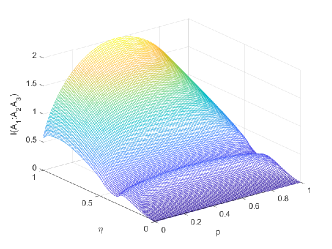
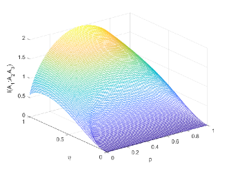
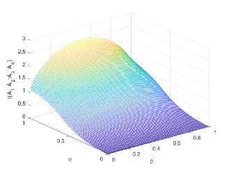
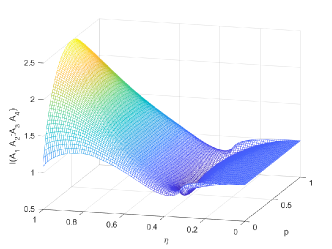
Example 5 (A single qubit at multiple times).
Let be a multiple time single qubit PDM with initial state with . Denote the channel responsible for the evolution of the system between times and by , and let be the depolarizing channel given by
where is the depolarization parameter. We then consider several cases of mutual information in time where is either the identity channel or the depolarizing channel for and , the results of which are plotted as functions of and in Figure 1.
Remark 1 (Lack of monotonicity).
While the spatial quantum mutual information satisfies monotonicity, namely, for every local operation on the system , local operations can either increase or decrease mutual information in time. In particular, while tracing out a subsystem of a multipartite spatial system essentially discards the information contained in , tracing out a subsystem of a multipartite dynamical system results in a redistribution of information across time to form a distinct dynamical system , where then has direct causal influence on . As such, the local operation of tracing out a subsystem of a dynamical system may result in an increase in the mutual information between different timelike separated subsystems, thus resulting in a failure of monotonicity.
IV A single qubit at two times: The general case
For a single qubit at two-times we obtain the following theorem, whose proof can be found in Appendix A.
Theorem 2.
Let be a 2-time PDM associated with a single qubit whose initial state is maximally mixed and which evolves according to a channel that is either unital or has Choi rank no greater than 2 between measurements. Then .
While we conjecture that holds for an arbitrary qubit at two times, our proof of Theorem 2 relies on the hypotheses that the initial state is maximally mixed and that the channel corresponding to the evolution between measurements is either unital or has Choi rank no greater than 2. We note that it follows from Theorem 1 that the bound also holds for arbitrary initial states provided that the evolution between measurements is unitary.
Assuming holds for an arbitrary qubit at two times, such a feature of temporal correlations is in stark contrast with the case of two qubits separated in space, which can achieve a maximum mutual information of 2 in the presence of entanglement Cerf and Adami (1997). This is a reflection of the fact that unlike the monogamy spatial correlations, a single qubit can be maximally correlated both with a qubit in its immediate future and it immediate past. In particular, given a 3-time measurement scenario, the qubit at time can violate CHSH inequalities both with the qubits at times and , which is a consequence of the fact that two-time correlation functions associated with Pauli observables are independent of initial conditions Brukner et al. (2004); Fritz (2010).
An interesting consequence of the bound for a qubit at two times, is that if a pair of spatially entangled qubits has a mutual information greater than 1, then it follows that the two qubits do not admit a dual description of being timelike separated. The converse to this statement however does not hold in general. In particular, a pair of spatially entangled qubits not admitting a dual description of being timelike separated can have mutual information less than one, as in the case of the entangled qubits described by the pure state for small .
We also note that it follows from Example 3 that the lower bound of for the mutual information in the context of Theorem 2 is achieved when a qubit evolves according to a completely depolarizing channel between measurements. This is consistent with the fact that all information about the initial measurement is lost in such a scenario. On the other hand, we know from Theorem 1 that the upper bound of 1 for is achieved when a maximally mixed qubit undergoes unitary evolution between the two measurements, which is consistent with the fact that no information is lost (or gained) under unitary evolution.
V Time-reversal Symmetry
For spatial mutual information it is always the case that , as there is no preferred directionality in space between spacelike separated systems. In particular, applying the swap transformation to a bipartite density matrix yields a density matrix which is physically indistinguishable from , so that .
When and are timelike separated the situation is more subtle, as a quantum channel establishing temporal correlations between and may be non-reversible due to noise. In such a case, the non-reversibility of is reflected in the associated PDM by the fact that the swap is not a PDM. However, when is in fact a PDM, so that , where and is a quantum channel from to , then is said to be a Bayesian inverse of the channel with respect to the state Parzygnat and Fullwood (2023). As such, the notion of a Bayesian inverse provides a novel form of reversibility for timelike separated quantum systems, even when the systems are temporally correlated via a noisy channel.
As solving for a Bayesian inverse involves solving a linear system, the number of solutions is either 0,1 or , with 0 corresponding to no Bayesian inverse existing, 1 corresponding to a unique Bayesian inverse and corresponding to the notion of Bayesian inverse being non-unique. However, in the case of non-uniqueness, given two Bayesian inverses and of with respect to , then it follows from the definition of Bayesian inverse that , so that the notion of a PDM corresponding to a time-reversal of the process described by is well-defined.
In the context of mutual information in time, suppose we have a PDM with Bayesian invertible with respect to , so that the swap , where and is a quantum channel from to corresponding to a Bayesian inverse of with respect to . Now since the eigenvalues of a matrix are invariant under the swap map , it follows that . Moreover, since and , we have
Thus, the existence of a Bayesian inverse of a channel establishes a symmetry in time which extends the symmetry of spatial mutual information into the time domain.
VI A Holevo Bound in Time
Suppose Alice sends a pure state to Bob with probability , after which Bob performs a measurement on corresponding to a POVM . Then the probability of the measurement outcome given the state is given by . If is a random variable associated with the probability distribution , and is a random variable associated with the probability distribution , then the classical mutual information is bounded above by the Holevo quantity given by
| (8) |
The inequality is referred to as the Holevo bound Holevo (1973), and thus provides a fundamental limit on the amount of classical information which may be extracted from an ensemble of quantum states. Moreover, if we form the joint classical-quantum state associated with Alice’s classical register and Bob’s random acquisition of the state , namely,
| (9) |
then it is straightforward to show that the mutual information associated with is such that . This, together with the Holevo bound, provides an operational interpretation for the quantum mutual information . In this section, we obtain analogous results for mutual information in time.
For this, we first note that from a dynamical perspective, the state is in fact the PDM given by , where is the channel given by and is the state given by . In such a 2-time scenario, the channel is then viewed as a channel from Alice to Bob. If Bob then makes two sequential measurements on , with the system evolving according to a channel between measurements, then it follows from (6) that the associated 3-time PDM (with and ) is then given by
| (10) |
where is the 2-time PDM associated with Bob’s sequential measurements. We then obtain the following:
Theorem 3.
Let be the 2-time PDM associated with Bob’s sequential measurements of , and let be the mutual information associated with the classical-quantum PDM given by (10). Then the following statements hold.
-
i.
.
-
ii.
If Bob’s system evolves unitarily between measurements, then , where is the Holevo quantity (8).
Proof.
First, we have and , so that
| (11) |
where denotes the Shannon entropy associated with the probability distribution . Now since is additive and orthogonally convex (as defined in the introduction), we have
Substituting into equation (11) then yields
| (12) |
which proves item i. Now if Bob’s system evolves according to a unitary channel between measurements, so that , it follows from (7) that . Moreover, as the spatiotemporal product is linear in , we have
where the final equation follows again from (7). It then follows from equation (12) that , which proves item ii. ∎
Now let be the random variable associated with Alice’s classical register, and let be the bivariate random variable corresponding to the joint statistics of Bob’s classical register when performing sequential measurements of the POVMs and . We assume that after a measurement outcome of when measuring that Bob’s system updates to (suitably normalized) for some fixed unitary which is independent of and . It then follows that the joint distribution corresponding to the bivariate random variable is given by , where the conditional distribution is given by
Now since the mapping given by
is a quantum channel, it follows from Lemma 1 of Appendix B that the mutual information between Alice’s classical register and the bivariate register corresponding to Bob’s sequential measurements is also bounded above by the Holevo quantity . Thus, it follows from Theorem 3 that
where again is the mutual information in time associated with the classical-quantum PDM given by (10). By taking a supremum over all possible POVMs and , it then follows that the amount of classical information that may be extracted from such sequential measurements is bounded above by the mutual information in time .
VII Concluding Remarks
In this work, we have employed the pseudo-density matrix formalism to define an extension of quantum mutual information into the time domain. Such a measure of quantum information naturally quantifies correlations between timelike separated quantum systems, and recovers the usual spatial mutual information for systems which admit a dual description of either being timelike or spacelike separated. We have proved such a notion of mutual information in time satisfies various properties one would expect from such a dynamical measure of information, highlighting the ways in which quantum correlations distinguish between space and time.
We note that while an alternative formulation of quantum mutual information for timelike separated systems has recently appeared in Glorioso et al. (2024), such a quantity is defined in terms of optimizing a relative entropy over all possible system-ancilla coupling schemes, resulting in a quantity which often diverges, even for systems consisting of a single qubit. From the dynamical perspective espoused in this work, the limitations of the aforementioned approach stem from the fact that a spatial notion of relative entropy is being utilized, rather than a dynamical extension of relative entropy using the entropy function .
As for the quantum mutual information in time defined in this work, we have shown that a single qubit at two times can never exceed a mutual information of . This is consistent with the fact that for two qubits to be correlated in time there must necessarily be a causal transfer of information between the two qubits via a quantum channel, and hence two timelike separated qubits can share at most one bit of information. An interesting consequence of such an upper bound for the mutual information between a qubit at two times, is that if two spatially separated qubits have mutual information exceeding 1, then it necessarily follows that the correlations between such qubits may not be realized in a dynamical setting where the two qubits are separated in time.
Another interesting aspect of quantum mutual information in time is that in all known 2-time examples it is non-negative, despite the fact that the entropy function is not subadditive on general hermitian matrices of unit trace. In particular, in Ref. Fullwood and Parzygnat (2023), an example of a unit trace bipartite Hermitian matrix was constructed whose marginals are density matrices, and yet
| (13) |
In such a case, is of the form with not a CPTP map, which the entropy function seems to be detecting via the failure of subadditivity (13).
Finally, it is worth noting that quantum mutual information in time may be used to define a notion of channel capacity for a quantum channel which is directly analogous to Shannon’s original definition in the classical case, i.e., by taking a supremum of mutual information with respect to all possible input states for the channel . It would be interesting then to compare such a notion of channel capacity with other notions of quantum capacity Lloyd (1997); Devetak (2005); Holevo (2020), especially since such a quantity is often computable.
VIII Acknowledgements
VV acknowledges support from the Templeton and the Gordon and Betty Moore foundations, and WZ would like to thank the Institute of Mathematical Science at Hainan University for hospitality during the course of this project.
References
- Cerf and Adami (1997) N. J. Cerf and C. Adami, “Negative entropy and information in quantum mechanics,” Phys. Rev. Lett. 79, 5194–5197 (1997).
- Nielsen and Chuang (2011) Michael A. Nielsen and Isaac L. Chuang, Quantum computation and quantum information, 10th ed. (Cambridge University Press, Cambridge, 2011) pp. xxvi+676.
- Cover and Thomas (2006) Thomas M. Cover and Joy A. Thomas, Elements of Information Theory (Wiley Series in Telecommunications and Signal Processing) (Wiley-Interscience, 2006).
- Fitzsimons et al. (2015) Joseph F. Fitzsimons, Jonathan A. Jones, and Vlatko Vedral, “Quantum correlations which imply causation,” Sci. Rep. 5, 18281 (2015), arXiv:1302.2731 [quant-ph] .
- Fullwood and Parzygnat (2024) James Fullwood and Arthur J. Parzygnat, “Operator representation of spatiotemporal quantum correlations,” (2024), arXiv:2405.17555 [quant-ph] .
- Marletto et al. (2021) Chiara Marletto, Vlatko Vedral, Salvatore Virzì, Alessio Avella, Fabrizio Piacentini, Marco Gramegna, Ivo Pietro Degiovanni, and Marco Genovese, “Temporal teleportation with pseudo-density operators: How dynamics emerges from temporal entanglement,” Sci. Adv. 7, eabe4742 (2021), arXiv:2103.12636 [quant-ph] .
- Zhao et al. (2018) Zhikuan Zhao, Robert Pisarczyk, Jayne Thompson, Mile Gu, Vlatko Vedral, and Joseph F. Fitzsimons, “Geometry of quantum correlations in space-time,” Phys. Rev. A 98, 052312 (2018), arXiv:1711.05955 [quant-ph] .
- Pisarczyk et al. (2019) Robert Pisarczyk, Zhikuan Zhao, Yingkai Ouyang, Vlatko Vedral, and Joseph F. Fitzsimons, “Causal limit on quantum communication,” Physical Review Letters 123 (2019), 10.1103/physrevlett.123.150502.
- Marletto et al. (2020) Chiara Marletto, Vlatko Vedral, Salvatore Virzì, Enrico Rebufello, Alessio Avella, Fabrizio Piacentini, Marco Gramegna, Ivo Pietro Degiovanni, and Marco Genovese, “Non-monogamy of spatio-temporal correlations and the black hole information loss paradox,” Entropy 22, 228 (2020).
- Marletto et al. (2019) Chiara Marletto, Vlatko Vedral, Salvatore Virzì, Enrico Rebufello, Alessio Avella, Fabrizio Piacentini, Marco Gramegna, Ivo Pietro Degiovanni, and Marco Genovese, “Theoretical description and experimental simulation of quantum entanglement near open time-like curves via pseudo-density operators,” Nature Communications 10 (2019), 10.1038/s41467-018-08100-1.
- Liu et al. (2024) Xiangjing Liu, Qian Chen, and Oscar Dahlsten, “Inferring the arrow of time in quantum spatiotemporal correlations,” Physical Review A 109 (2024), 10.1103/physreva.109.032219.
- Liu et al. (2023) Xiangjing Liu, Yixian Qiu, Oscar Dahlsten, and Vlatko Vedral, “Quantum causal inference with extremely light touch,” (2023), arXiv:2303.10544 [quant-ph] .
- Song et al. (2024) Minjeong Song, Varun Narasimhachar, Bartosz Regula, Thomas J. Elliott, and Mile Gu, “Causal classification of spatiotemporal quantum correlations,” Phys. Rev. Lett. 133, 110202 (2024), arXiv:2306.09336 [quant-ph] .
- Jia et al. (2023) Zhian Jia, Minjeong Song, and Dagomir Kaszlikowski, “Quantum space-time marginal problem: global causal structure from local causal information,” New J. Phys. 25, 123038 (2023).
- Parzygnat and Fullwood (2024) Arthur J. Parzygnat and James Fullwood, “Time-symmetric correlations for open quantum systems,” (2024), arXiv:2407.11123 [quant-ph] .
- French (1968) A. P. French, Special Relativity (W. W. Norton & Company, 1968).
- Hawking and Ellis (1973) Stephen W. Hawking and George F. R. Ellis, The Large Scale Structure of Space-Time, Cambridge Monographs on Mathematical Physics (Cambridge University Press, 1973).
- Fullwood and Parzygnat (2023) James Fullwood and Arthur J. Parzygnat, “On dynamical measures of quantum information,” (2023), arXiv:2306.01831 [quant-ph] .
- Parzygnat et al. (2023) Arthur J. Parzygnat, Tadashi Takayanagi, Yusuke Taki, and Zixia Wei, “SVD entanglement entropy,” JHEP 12, 123 (2023), arXiv:2307.06531 [hep-th] .
- Tu et al. (2022) Yi-Ting Tu, Yu-Chin Tzeng, and Po-Yao Chang, “Rényi entropies and negative central charges in non-hermitian quantum systems,” SciPost Physics 12 (2022), 10.21468/scipostphys.12.6.194.
- Salek et al. (2014) Sina Salek, Roman Schubert, and Karoline Wiesner, “Negative conditional entropy of postselected states,” Phys. Rev. A 90, 022116 (2014), arXiv:1305.0932 [quant-ph] .
- Holevo (1973) A. S. Holevo, “Bounds for the quantity of information transmitted by a quantum communication channel,” Problemy Peredači Informacii 9, 3–11 (1973).
- Parzygnat and Fullwood (2023) Arthur J. Parzygnat and James Fullwood, “From time-reversal symmetry to quantum Bayes’ rules,” PRX Quantum 4, 020334 (2023), arXiv:2212.08088 [quant-ph] .
- Horsman et al. (2017) Dominic Horsman, Chris Heunen, Matthew F. Pusey, Jonathan Barrett, and Robert W. Spekkens, “Can a quantum state over time resemble a quantum state at a single time?” Proc. R. Soc. A 473, 20170395 (2017), arXiv:1607.03637 [quant-ph] .
- Jamiołkowski (1972) Andrzej Jamiołkowski, “Linear transformations which preserve trace and positive semidefiniteness of operators,” Rep. Math. Phys. 3, 275–278 (1972).
- Fullwood (2023a) James Fullwood, “Quantum dynamics as a pseudo-density matrix,” (2023a), arXiv:2304.03954 [quant-ph] .
- Werner (1989) Reinhard F. Werner, “Quantum states with Einstein-Podolsky-Rosen correlations admitting a hidden-variable model,” Phys. Rev. A 40, 4277–4281 (1989).
- Brukner et al. (2004) Caslav Brukner, Samuel Taylor, Sancho Cheung, and Vlatko Vedral, “Quantum entanglement in time,” (2004), arXiv:quant-ph/0402127 [quant-ph] .
- Brody and Hughston (2024) Dorje C. Brody and Lane P. Hughston, “Decoherence implies information gain,” (2024), arXiv:2402.16740 [quant-ph] .
- Fritz (2010) Tobias Fritz, “Quantum correlations in the temporal Clauser-Horne-Shimony-Solt (CHSH) scenario,” New J. Phys. 12, 083055 (2010), arXiv:1005.3421 [quant-ph] .
- Glorioso et al. (2024) Paolo Glorioso, Xiao-Liang Qi, and Zhenbin Yang, “Space-time generalization of mutual information,” JHEP 05, 338 (2024), arXiv:2401.02475 [quant-ph] .
- Lloyd (1997) Seth Lloyd, “Capacity of the noisy quantum channel,” Physical Review A 55, 1613–1622 (1997).
- Devetak (2005) I. Devetak, “The private classical capacity and quantum capacity of a quantum channel,” IEEE Trans. Info. Theor. 51, 44–55 (2005).
- Holevo (2020) A. S. Holevo, “Quantum channel capacities,” Quantum Electron. 50, 440–446 (2020).
- Ruskai et al. (2002) Mary Beth Ruskai, Stanislaw Szarek, and Elisabeth Werner, “An analysis of completely-positive trace-preserving maps on ,” Linear Algebra Its Appl. 347, 159–187 (2002).
- Parzygnat et al. (2024) Arthur Parzygnat, James Fullwood, Francesco Buscemi, and Giulio Chiribella, “Virtual quantum broadcasting,” Phys. Rev. Lett. 132, 110203 (2024), arXiv:2310.13049 [quant-ph] .
- Fullwood (2023b) James Fullwood, “General covariance for quantum states over time,” (2023b), arXiv:2311.00162 [quant-ph] .
- Marshall et al. (2010) Albert W. Marshall, Ingram Olkin, and Barry C. Arnold, Inequalities: Theory of Majorization and Its Applications (Springer New York, NY, 2010).
Methods testing
Quantum Mutual Information in Time
— Supplementary Material —
Appendix A Proof of Theorem 2
Let and denote quantum systems corresponding to a single qubit at times and with , and suppose the system which is initially in the state evolves according to a quantum channel between measurements at times and . In such a case, the mutual information between the qubit at times and is given by
| (14) |
where
| (15) |
and
for all Hermitian matrices . In this section, we will prove Theorem 2, which states that if is maximally mixed, and if is either unital or of Choi rank no more than 2, then . We note that under the assumption that is maximally mixed, it follows from (15) that
| (16) |
for every channel .
A.1 Reduction to
Let be a quantum channel. As an arbitrary density matrix may be written with respect to the Pauli basis as
with and , it can be shown that the quantum channel takes the form
where and . Thus, a matrix representation of the channel with respect to the Pauli basis is of the form Ruskai et al. (2002)
| (17) |
Moreover, one can show that there exist unitary channels and such that
| (18) |
where the matrix representation of is given by
| (19) |
Now let be the maximally mixed state, and let and be the PDMs given by and . Since , the covariance property of PDMs Parzygnat et al. (2024); Fullwood (2023b) yields
| (20) |
where is the Hilbert-Schmidt adjoint of . If is the unitary operator such that for all , then it follows that
thus by (20) we have
Moreover, since we have . It then follows by the unitary-invariance of that and . Now let and denote the mutual information associated with and respectively. We then have
thus for any qubit channel with initial state . As such, when proving Theorem 2, we may compute in terms of , which we’ll refer to as ‘ reduction to ’.
A.2 Unital channels
In this section, we consider the case when is a unital channel. Before proceeding with the proof, we recall that a real vector is said to majorize a real vector , written if and only if for , where denotes the components of in decreasing order and denotes the components of in decreasing order. A function is then said to be Schur-Concave if and only if Marshall et al. (2010).
So now suppose is a unital channel, in which case the vector t in (17) is zero. This then implies that is a Pauli channel, i.e., for some probability vector and for all . Since is unital, it follows that for maximally mixed, so that the associated mutual information is then given by
| (21) |
As for the associated PDM , we have
| (22) |
from which it follows that the eigenvalues of are
We now consider two cases:
-
(1)
If all for all , then the eigenvalues of are all non-negative and is a dual state, thus . We now show . For this, let denote the probability vector of eigenvalues of with . Since for it follows that for , thus the probability vector majorizes , hence since the Shannon entropy is Schur-Concave. It then follows that by (21).
-
(2)
If there exists a , with loss of generality, assume that and for . We then have
(23) where we use the notion when we want to emphasize that we may view as a function of . We now wish to bound from above and below. To obtain a minimum value of , we only need compute the minimum value of for every fixed , i.e.,
Now for a fixed , it follows from (23) that is minimized by finding which minimize the entropy of the vector . As for , it follows that the vector i.e. and , majorizes , hence
so that
(24) Therefore, for every fixed , we always have , thus . To bound from above, notice that the vector majorizes the vector and can always be attained by choosing for every fixed , hence
Moreover, since
it follows that , thus by (21).
By reduction to , it follows that if is unital, then , as desired. We note that in such a case we have if and only if is the completely depolarizing channel, and if and only if there are at least two in equal to zero, i.e., when the Choi rank of is no more than 2.
A.3 Channels of Choi rank no greater than 2
In this section, we consider the case when the Choi rank of is no greater than 2. In such a case, one may show that for the matrix representation of the channel as given by (19), we have that , and . Therefore, let and , so that the matrix may be written in the form
| (25) |
with . It is then straightforward to verify that with respect to this parameterization, admits the Kraus representation given by Ruskai et al. (2002)
where
| (26) | ||||
Since is non-unital, we have , so that for the PDM is then given by
| (27) |
hence the eigenvalues of are
It then follows that , which yields
Since is a density matrix , thus . By reduction to , it follows that if the Choi rank of is no greater than 2, then , as desired.
Appendix B Holevo bound for sequential measurements
In this section, we prove a lemma which implies that the Holevo bound also holds for sequential measurements on an ensemble of quantum states.
Lemma 1.
Let be a random variable whose values are associated with a probability distribution , let be a family of bivariate probability distributions conditioned on , and suppose there exists a quantum channel and a collection of density matrices such that for all .Then for every bivariate random variable whose values are associated with the bivariate distribution ,
where is the mutual information of the random variables and .
Proof.
By the Stinespring dilation theorem there exists an isometry and an operator such that for all and for all . Now let be the density matrix given by
and let be the density matrix given by
where . We then have
thus monotonicity of (spatial) quantum mutual information implies , where is the quantum mutual information associated with the density matrix and is the quantum mutual information associated with the density matrix . Moreover, we have
and since , we then have
as desired. ∎