Fermionic Mean-Field Theory as a Tool for Studying Spin Hamiltonians

Abstract

The Jordan–Wigner transformation permits one to convert spin $1/2$ operators into spinless fermion ones, or vice versa. In some cases, it transforms an interacting spin Hamiltonian into a noninteracting fermionic one which is exactly solved at the mean-field level. Even when the resulting fermionic Hamiltonian is interacting, its mean-field solution can provide surprisingly accurate energies and correlation functions. Jordan–Wigner is, however, only one possible means of interconverting spin and fermionic degrees of freedom. Here, we apply several such techniques to the XXZ and $J_{1}\text{--}J_{2}$ Heisenberg models, as well as to the pairing or reduced BCS Hamiltonian, with the aim of discovering which of these mappings is most useful in applying fermionic mean-field theory to the study of spin Hamiltonians.

I Introduction

It is textbook material [1, 2] that the Jordan–Wigner (JW) transformation [3] can convert certain interacting Hamiltonians of spin 1/2 systems into noninteracting (therefore exactly solvable) Hamiltonians of spinless fermions. Perhaps less appreciated is that even when the JW transformation produces an interacting fermionic Hamiltonian, it can nevertheless be solved at the mean-field level with moderate computational cost and good accuracy [4, 5, 6, 7, 8, 9, 10, 11, 12, 13].

Historically, the JW mapping was the first transformation used to relate spin 1/2 objects to fermions. Recently, the prospect of simulating fermionic systems on quantum devices has reignited interest in such mappings [14, 15, 16, 17], largely due to the parallels between qubits and spin 1/2 systems. Representing many-fermion problems on a quantum computer requires a mapping from fermions to qubits. Although the inverse JW transformation is a natural choice for this purpose, the past several years have seen the development of a variety of alternatives [14, 18, 19, 20, 21, 22, 23, 24, 25, 26, 27, 28].

In this work, we focus on a subset of these alternative mappings and apply them in the other direction. That is, given a transformation converting spinless fermions to spin 1/2 objects, we can invert the mapping to convert spin 1/2 objects to spinless fermions, thereby enabling the solution of interacting spin Hamiltonians using fermionic methods. Of course, the inversion of these mappings is not an entirely trivial task and the resulting fermionic Hamiltonians can be very exotic, but we aim to survey the landscape and discern which, if any, of the many spin-to-fermion mappings we will consider might be particularly useful.

To help orient the reader, we will begin with a quick survey of the spin-to-fermion transformations that we will consider in this work. We certainly cannot do full justice to this topic here, but we hope to provide a reasonably concise summary of these ideas. Likewise, because the Hamiltonians we obtain after the spin-to-fermion transformation are generally quite unusual, we must employ equally unusual mean-field methods to solve them, and we also provide a brief introduction to the general Hartree–Fock–Bogoliubov–Fukutome (HFBF) mean-field theory [29, 30, 31, 32] we use to tackle these problems.

II Spin-to-Fermion Transformations

The Hilbert space for a spin 1/2 object is spanned by two states: $\ket{\uparrow}$ and $\ket{\downarrow}$. The same is true for the Hilbert space of a spinless fermion, spanned by states $\ket{0}$ and $\ket{1}$ in the occupation number representation. Since the Hilbert spaces have the same size, we can map states for a single spinless fermion onto states for a single spin 1/2, and vice versa. The only real difficulty in extending these ideas to map states for $M$ fermions onto states for $M$ spins is that operators acting on different fermions anticommute, while operators acting on different spins commute. This idea was discussed by Jordan and Wigner in 1928 [3], but as we have said, a plethora of different mappings have since been introduced. Here, we want to summarize those which we will explore in this work.

II.1 Notation, and Majorana and Pauli Operators

It will prove helpful to establish our basic concepts and notation first. The bare fermionic creation and annihilation operators for level $p$ will be denoted as $c_{p}^{\dagger}$ and $c_{p}$, respectively, and they interconvert the two fermionic states, via

$$c_{p}^{\dagger}\ket{0_{p}} =\ket{1_{p}},$$ (1a)

$$c_{p}\ket{1_{p}} =\ket{0_{p}}.$$ (1b)

These operators obey canonical anticommutation relations:

$$\{c_{p},c_{q}\} =0,$$ (2a)

$$\{c_{p},c_{q}^{\dagger}\} =\delta_{pq},$$ (2b)

where $\{A,B\}=AB+BA$ is the anticommutator. The number operator $n_{p}=c_{p}^{\dagger}\,c_{p}$ determines whether level $p$ is occupied or empty.

We can draw a close analogy between these fermionic operators and the spin operators. The spin raising and lowering operators, $S_{p}^{+}$ and $S_{p}^{-}$, interconvert the two spin states:

$$S_{p}^{+}\ket{\downarrow_{p}} =\ket{\uparrow_{p}},$$ (3a)

$$S_{p}^{-}\ket{\uparrow_{p}} =\ket{\downarrow_{p}}.$$ (3b)

Where the fermionic states $\ket{0_{p}}$ and $\ket{1_{p}}$ are eigenstates of the number operator $n_{p}$ with eigenvalues 0 and 1, respectively, the spin states $\ket{\uparrow_{p}}$ and $\ket{\downarrow_{p}}$ are instead eigenstates of the operator $S_{p}^{z}$ with respective eigenvalues $+1/2$ and $-1/2$. However, the spin operators obey $\mathfrak{su}(2)$ commutation rules:

$$[S_{p}^{+},S_{q}^{-}] =2\,\delta_{pq}\,S_{p}^{z},$$ (4a)

$$[S_{p}^{z},S_{q}^{\pm}] =\pm\delta_{pq}\,S_{p}^{\pm}.$$ (4b)

We also have the $x$ and $y$ spin operators, which we can obtain from

$$S_{p}^{\pm}=S_{p}^{x}\pm\mathrm{i}\,S_{p}^{y},$$ (5)

which together with $S_{p}^{z}$ satisfy

$$[S_{p}^{i},S_{q}^{j}]=\mathrm{i}\,\delta_{pq}\,\epsilon_{ijk}\,S_{p}^{k},$$ (6)

where $i,j,k\in\{x,y,z\}$. Since we are working purely with spin 1/2, we also have that

$$\left(S_{p}^{i}\right)^{2}=1/4.$$ (7)

It is helpful for our purposes to define the Majorana operators $\gamma_{1,p}$ and $\gamma_{2,p}$ as

$$\gamma_{1,p} =c_{p}+c_{p}^{\dagger},$$ (8a)

$$\gamma_{2,p} =\mathrm{i}\,\left(c_{p}-c_{p}^{\dagger}\right).$$ (8b)

These operators are Hermitian (e.g., $\gamma_{1,p}^{\dagger}=\gamma_{1,p}$), with $\gamma_{1,p}^{2}=\gamma_{2,p}^{2}=1$, and the different Majorana operators all anticommute with one another. Notice that

$$\mathrm{i}\,\gamma_{1,p}\,\gamma_{2,p}=1-2\,n_{p}.$$ (9)

Similarly, we can define Pauli operators, $\sigma_{p}^{i}$, from

$$S_{p}^{i}=\frac{1}{2}\,\sigma_{p}^{i}.$$ (10)

Like the Majoranas, the Pauli operators are Hermitian and are involutions ($O^{2}=1$). Paulis on different sites commute, while for Paulis on the same site we may use

$$\sigma_{p}^{i}\,\sigma_{p}^{j}=\delta_{ij}\,1+\mathrm{i}\,\epsilon_{ijk}\,\sigma_{p}^{k}.$$ (11)

II.2 The Jordan–Wigner Transformation

Based on the similarities we have noted between the spin operators on the one hand and the fermionic operators on the other, Jordan and Wigner [3] suggested a mapping which, when transforming fermions to spins, we may write as

$$c_{p}^{\dagger} \underset{\text{JW}}{\mapsto}S_{p}^{+}\,\phi_{p}^{z},$$ (12a)

$$c_{p} \underset{\text{JW}}{\mapsto}S_{p}^{-}\,\phi_{p}^{z},$$ (12b)

$$\phi_{p}^{z} =\prod_{q<p}(-2\,S_{q}^{z}),$$ (12c)

which just means that for states we map

$$\ket{0_{p}} \underset{\text{JW}}{\mapsto}\ket{\downarrow_{p}},$$ (13a)

$$\ket{1_{p}} \underset{\text{JW}}{\mapsto}\ket{\uparrow_{p}}.$$ (13b)

The Hermitian operator $\phi_{p}^{z}$ is the JW string and is responsible for yielding the correct anticommutation relationships. Note that in the quantum computing community, it is common to map $\ket{0_{p}}$ to $\ket{\uparrow_{p}}$, which means that the creation operator $c_{p}^{\dagger}$ maps to $S_{p}^{-}\,\hat{\phi}_{p}^{z}$, where $\hat{\phi}_{p}^{z}$ does not have signs in defining the JW strings.

This transformation can be inverted to map spin operators to fermions:

$$S_{p}^{+} \underset{\text{JW}}{\mapsto}c_{p}^{\dagger}\,\tilde{\phi}_{p},$$ (14a)

$$S_{p}^{-} \underset{\text{JW}}{\mapsto}c_{p}\,\tilde{\phi}_{p},$$ (14b)

$$S_{p}^{z} \underset{\text{JW}}{\mapsto}n_{p}-\frac{1}{2},$$ (14c)

$$\tilde{\phi}_{p} =\prod_{q<p}\mathrm{e}^{\mathrm{i}\,\pi\,n_{q}}=\prod_{q<p}\left(1-2\,n_{q}\right).$$ (14d)

The JW transformation has the virtue of simplicity. Moreover, because it maps the total $S^{z}$ operator into the total number operator $N$ (modulo an irrelevant shift) it converts fermionic Hamiltonians with number symmetry into spin Hamiltonians with $S^{z}$ symmetry and vice versa.

We note that the JW transformation depends on the labeling of the sites or fermions, because in the strings for level $p$ we have products over $q<p$. This dependence is of no practical significance if the Hamiltonian is solved exactly, but when mapped Hamiltonians are solved approximately, the result may depend on the ordering of the spins or fermions. One can take advantage of this additional degree of freedom and choose the ordering that minimizes a given cost function, such as the number of Pauli operators in the transformed Hamiltonian [33]. Alternatively, there is an extension of the JW transformation [34] which, at the mean-field level, eliminates this dependency [13].

Finally, we have given the JW transformation in terms of bare fermion and spin operators. In terms of Majorana and Pauli operators, we have instead

$$\gamma_{1,p} \underset{\text{JW}}{\mapsto}\sigma_{p}^{x}\,\phi_{p}^{z},$$ (15a)

$$\gamma_{2,p} \underset{\text{JW}}{\mapsto}\sigma_{p}^{y}\,\phi_{p}^{z},$$ (15b)

$$\phi_{p}^{z} =\prod_{q<p}\left(-\sigma_{q}^{z}\right),$$ (15c)

$$\sigma_{p}^{x} \underset{\text{JW}}{\mapsto}\gamma_{1,p}\,\tilde{\phi}_{p},$$ (15d)

$$\sigma_{p}^{y} \underset{\text{JW}}{\mapsto}\gamma_{2,p}\,\tilde{\phi}_{p},$$ (15e)

$$\sigma_{p}^{z} \underset{\text{JW}}{\mapsto}-\mathrm{i}\,\gamma_{1,p}\,\gamma_{2,p},$$ (15f)

$$\tilde{\phi}_{p} =\prod_{q<p}\left(\mathrm{i}\,\gamma_{1,q}\,\gamma_{2,q}\right).$$ (15g)

II.3 The Parity Transformation

The parity ($\Pi$) transformation [19] is in some sense the dual companion of the JW transformation. In the JW case, we map the occupation of fermionic level $p$ into the direction of spin $p$. Because fermions anticommute, occupation numbers alone are not enough to distinguish states, and we must also determine sign information, or parity. In the JW case, the sign information through site $p$ is found by looking at the occupations of all levels $q<p$. Thus, in JW, occupation is encoded locally but parity is encoded nonlocally. In contrast, the $\Pi$ transformation encodes parity information locally, but then must encode occupancy nonlocally.

Specifically, we have

$$\gamma_{1,p} \underset{\Pi}{\mapsto}\psi_{p}^{x}\,\sigma_{p-1}^{z},$$ (16a)

$$\gamma_{2,p} \underset{\Pi}{\mapsto}-\mathrm{i}\,\psi_{p}^{x}\,\sigma_{p}^{z},$$ (16b)

$$\psi_{p}^{x} =\prod_{q\geq p}\sigma_{q}^{x}.$$ (16c)

Inverting this transformation yields

$$\sigma_{p}^{x} \underset{\Pi}{\mapsto}\mathrm{i}\,\gamma_{2,p}\,\gamma_{1,p+1},$$ (17a)

$$\sigma_{p}^{y} \underset{\Pi}{\mapsto}\mathrm{i}\,\tilde{\phi}_{p}\,\gamma_{1,p}\,\gamma_{1,p+1},$$ (17b)

$$\sigma_{p}^{z} \underset{\Pi}{\mapsto}\mathrm{i}\,\tilde{\phi}_{p}\,\gamma_{1,p}\,\gamma_{2,p}.$$ (17c)

With $M$ sites, counting from 1, we must define $\sigma_{0}^{z}$ and $\gamma_{1,M+1}$, which we take to be, respectively,

$$\sigma_{0}^{z} \equiv 1,$$ (18a)

$$\gamma_{1,M+1} \equiv\Pi=\tilde{\phi}_{M+1}=\mathrm{e}^{\mathrm{i}\,\pi\,N}.$$ (18b)

The operator $\Pi$ is the global number parity operator and acts on number eigenstates to return eigenvalues of $\pm 1$, depending on whether the state has an even (eigenvalue $+1$) or an odd (eigenvalue $-1$) number of particles. The presence of this number parity operator leads us to use the symbol $\Pi$ to refer also to the parity transformation.

Note that the JW transformation singles out the $z$ axis for special treatment, in that $\sigma_{p}^{z}$ is the Pauli operator which does not get a string when it is mapped, while the $\Pi$ transformation instead singles out the $x$ axis. Of course these choices of axes are merely a matter of convention, and can be rotated arbitrarily. It will be useful to refer to a “rotated parity” transformation which, like the JW mapping, singles out the $z$ axis for special treatment. This rotated $\Pi$ transformation, denoted by $\Pi_{R}$, just has $\{\sigma_{p}^{x},\sigma_{p}^{y},\sigma_{p}^{z}\}\to\{\sigma_{p}^{z},\sigma_{p}^{x},\sigma_{p}^{y}\}$ so that

$$\gamma_{1,p} \underset{\Pi_{R}}{\mapsto}\psi_{p}^{z}\,\sigma_{p-1}^{y},$$ (19a)

$$\gamma_{2,p} \underset{\Pi_{R}}{\mapsto}-\mathrm{i}\,\psi_{p}^{z}\,\sigma_{p}^{y},$$ (19b)

$$\psi_{p}^{z} =\prod_{q\geq p}\sigma_{k}^{z},$$ (19c)

$$\sigma_{p}^{x} \underset{\Pi_{R}}{\mapsto}\mathrm{i}\,\tilde{\phi}_{p}\,\gamma_{1,p}\,\gamma_{1,p+1},$$ (19d)

$$\sigma_{p}^{y} \underset{\Pi_{R}}{\mapsto}\mathrm{i}\,\tilde{\phi}_{p}\,\gamma_{1,p}\,\gamma_{2,p},$$ (19e)

$$\sigma_{p}^{z} \underset{\Pi_{R}}{\mapsto}\mathrm{i}\,\gamma_{2,p}\,\gamma_{1,p+1},$$ (19f)

$$\sigma_{0}^{y} \equiv 1.$$ (19g)

Note that the $\Pi$ transformation converts a single Pauli into a product of two Majoranas, possibly times a string. Since the string is itself a product of an even number of Majoranas, it seems like the $\Pi$ transformation should convert each Pauli to a fermionic operator which conserves number parity (since operators which are products of an even number of Majoranas conserve number parity). Unfortunately, at the $M^{\text{th}}$ site, we instead have, for the $\Pi$ transformation, $\sigma_{M}^{x}\mapsto\mathrm{i}\,\gamma_{2,M}\,\Pi$, and this operator changes an even number parity state into an odd number parity state, and vice versa. Something similar happens for $\sigma_{M}^{y}$. This means that spin Hamiltonians which contain these two operators will typically transform into fermionic Hamiltonians which break number parity symmetry.

II.4 The Bravyi–Kitaev and Sierpinski Transformations

The JW and $\Pi$ transformations both use the spin state to represent the information of the occupied orbitals in the corresponding fermionic states, but they do so with a sub-optimal cost due to the need for long strings of Pauli operators to handle occupation changes and phase retrieval. In both cases, evaluating changes in occupation and fermionic phases scales as $M$, for $M$ spin states. However, we can choose our encoding so that it reduces the lookup and update cost associated with the phase and occupation number of fermionic states. The Bravyi–Kitaev (BK) transformation [14, 19] achieves this goal with $\mathcal{O}(\log_{2}(M))$ scaling in the following way.

The BK transformation improves the encoding efficiency by iteratively bisecting sets of fermionic modes to store partial sums in spin states. This approach enables efficient parity checks for any set of modes while minimizing the number of spins that need to be flipped during raising or lowering operations [35]. The transformation is captured by a matrix $\beta_{M}^{\text{BK}}$, which linearly maps Fock basis states $\ket{f}$ to encoded spin states $\ket{\sigma}^{\text{BK}}$ using addition modulo $2$. This matrix is illustrated below for $M=8$:

$$\ket{\sigma}^{\text{BK}}\equiv\beta_{M}^{\text{BK}}\ket{f}:=\begin{pmatrix}1&&&&&&&\\ 1&1&&&&&&\\ &&1&&&&&\\ 1&1&1&1&&&&\\ &&&&1&&&\\ &&&&1&1&&\\ &&&&&&1&\\ 1&1&1&1&1&1&1&1\\ \end{pmatrix}\begin{pmatrix}n_{1}\\ n_{2}\\ n_{3}\\ n_{4}\\ n_{5}\\ n_{6}\\ n_{7}\\ n_{8}\end{pmatrix},$$ (20)

resulting in

$$\begin{pmatrix}\sigma_{1}\\ \sigma_{2}\\ \sigma_{3}\\ \sigma_{4}\\ \sigma_{5}\\ \sigma_{6}\\ \sigma_{7}\\ \sigma_{8}\end{pmatrix}=\begin{pmatrix}n_{1}\\ n_{1}+n_{2}\\ n_{3}\\ n_{1}+n_{2}+n_{3}+n_{4}\\ n_{5}\\ n_{5}+n_{6}\\ n_{7}\\ n_{1}+n_{2}+n_{3}+n_{4}+n_{5}+n_{6}+n_{7}+n_{8}\end{pmatrix}.$$ (21)

All the information needed to replicate the group action of the fermionic raising and lowering operators is accessible from these spins. For each mode $i$, there are three sets of spin indices to consider. The Update set $U(i)$, comprises the spin sites needed to flip if the occupation of fermionic mode $i$ is changed. The Parity set $P(i)$, the minimum set of spins required to compute the parity of fermionic modes up to $i-1$. The Flip set $F(i)$, i.e., the smallest set of additional spin states needed to determine whether the $i$th spin state is equal to the $i$th fermionic occupation number or its opposite. For ease of notation, an operator with the subscript set $\mathcal{S}$ will be taken to mean “the tensor product of this operator on each element in $\mathcal{S}$” where appropriate; e.g., $(\sigma^{z})_{\mathcal{S}}=\prod_{s\in\mathcal{S}}(\sigma^{z})_{s}$.

To know whether to associate $c^{\dagger}_{i}$ with $S^{+}_{i}$ or $S^{-}_{i}$, consider the projection operators onto spaces of even or odd parity over a set $\mathcal{S}$:

$$\begin{split}E_{S}=\frac{1}{2}(I+(\sigma^{z})_{\mathcal{S}})\qquad O_{S}=\frac{1}{2}(I-(\sigma^{z})_{\mathcal{S}})\end{split}$$ (22)

and incorporate the knowledge from the Flip set to guarantee that the correct association is made with the new BK spin raising and lowering operators:

$$\begin{split}\Pi^{+}_{i}&=S^{+}_{i}\otimes E_{F(i)}-S^{-}_{i}\otimes O_{F(i)}\\ &=\frac{1}{2}\left((\sigma^{x})_{i}\otimes(\sigma^{z})_{F(i)}-(\mathrm{i}\,\sigma^{y})_{i}\right)\\ \Pi^{-}_{i}&=S^{-}_{i}\otimes E_{F(i)}-S^{+}_{i}\otimes O_{F(i)}\\ &=\frac{1}{2}\left((\sigma^{x})_{i}\otimes(\sigma^{z})_{F(i)}+(\mathrm{i}\,\sigma^{y})_{i}\right)\end{split}$$ (23)

Finally, with properly considered BK spin raising and lowering operators, and Update, Parity, and Flip sets, it is possible to define the fermionic creation and annihilation operators, as

$$\begin{split}c^{\dagger}_{i}&\underset{\text{BK}}{\mapsto}(\sigma^{z})_{P(i)}\otimes(\sigma^{x})_{U(i)}\otimes\Pi^{+}_{i},\\ c_{i}&\underset{\text{BK}}{\mapsto}(\sigma^{z})_{P(i)}\otimes(\sigma^{x})_{U(i)}\otimes\Pi^{-}_{i}.\end{split}$$ (24)

This formalism is completely generic. The only thing that determines the representation of the encoding is the occupation storage matrix $\beta_{M}$. For JW, this is the identity matrix, while for the $\Pi$ transformation, it is the lower-diagonal matrix with all 1s.

The bisections in the construction of the BK encoding matrix $\beta^{\text{BK}}_{M}$ ensure $O(\log_{2}(M))$ scaling for all three Update, Parity, and Flip sets. Meanwhile, the straightforward nature of the JW encoding matrix $\beta^{\text{JW}}_{M}$ allows for $O(1)$ size Update and Flip sets, but then requires an $O(M)$ size Parity set. Similarly, the $\Pi$ encoding matrix $\beta^{\Pi}_{M}$ allows for $O(1)$ size Parity and Flip sets, but then requires an $O(M)$ size Update set.

In the recently introduced Sierpinski tree (S) encoding [28], the authors extend the framework and define a $\beta^{S}_{M}$ which yields an encoding equivalent to the optimal ternary trees encoding [23], with the added advantage that the fermionic Fock states are mapped to spin basis states. In this case, the partial sums are allocated according to trisections, reflecting the fact that we get three anticommuting Pauli operators per spin site. This is illustrated for $M=13$:

$$\beta^{\text{S}}_{M}:=\setcounter{MaxMatrixCols}{13}\begin{pmatrix}1\\ 1&1&1\\ &&1\\ &&&1\\ 1&1&1&1&1&1&1&1&1\\ &&&&&1\\ &&&&&&1\\ &&&&&&1&1&1\\ &&&&&&&&1\\ &&&&&&&&&1\\ &&&&&&&&&1&1&1&\\ &&&&&&&&&&&1&\\ &&&&&&&&&&&&1\end{pmatrix}$$ (25)

This allows us to get Update, Parity, and Flip sets all of size $O(\log_{3}(M))$, an improvement still on BK which is provably optimal when $2M+1$ is a power of 3.

III Fermionic Mean-Field Methods

Fermionic mean-field theory is a surprisingly complex topic. Frequently when one hears the term, one envisions Hartree–Fock (HF), in which the bare fermionic operators $c$ and $c^{\dagger}$ are replaced by a transformed set of operators $a$ and $a^{\dagger}$, respectively, where

$$a_{p}^{\dagger}=\sum_{q}U_{qp}\,c_{q}^{\dagger}$$ (26)

and where the matrix $\boldsymbol{U}$ is unitary so that the transformation remains canonical. The mean-field state is then the product of an occupied set of $N$ creation operators acting on the physical vacuum $\ket{-}$:

$$\ket{\Phi_{\mathrm{HF}}}=\prod_{i=1}^{N}a_{i}^{\dagger}\ket{-},$$ (27)

and the resulting energy, defined as an expectation value, is minimized with respect to $\boldsymbol{U}$. It is convenient to represent $\boldsymbol{U}$ as the exponential of an antihermitian one-body matrix $\boldsymbol{\tau}$, and this is closely related to the Thouless representation [36] of the HF wave function, in which we write

$$\ket{\Phi_{\mathrm{HF}}} =\mathrm{e}^{\tau}\ket{\Phi_{0}},$$ (28a)

$$\tau =\sum_{ia}\left(\tau_{i}^{a}\,c_{a}^{\dagger}\,c_{i}-h.c.\right),$$ (28b)

$$\ket{\Phi_{0}} =\prod_{i}c_{i}^{\dagger}\,\ket{-},$$ (28c)

where $\ket{\Phi_{0}}$ is some suitably chosen reference; the index $i$ runs over levels occupied in $\ket{\Phi_{0}}$ and $a$ runs over levels empty in $\ket{\Phi_{0}}$.

It is frequently more convenient to use a non-unitary representation instead:

$$\ket{\Phi_{\mathrm{HF}}} =\mathcal{N}\,\mathrm{e}^{T}\ket{\Phi_{0}},$$ (29a)

$$T =\sum_{ia}T_{i}^{a}\,c_{a}^{\dagger}\,c_{i},$$ (29b)

where $\mathcal{N}$ is a normalization constant. So long as $\braket{\Phi_{0}}{\Phi_{\mathrm{HF}}}\neq 0$, this non-unitary approach is possible, though in practice we require the overlap $\braket{\Phi_{0}}{\Phi_{\mathrm{HF}}}$ to be sufficiently large so as to stave off numerical difficulties.

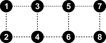
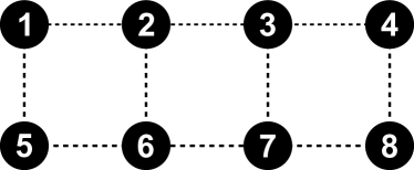
Figure 1: Labeling schemes for quasi-1D lattices. Left: the “$2\times n$” labeling for $n=4$. Right: the “$n\times 2$” labeling for $n=4$.

When the interaction is purely repulsive, HF is the optimal fermionic mean-field [37]. Interactions with attractive components, however, can lead to mean-field solutions with spontaneous number symmetry breaking. This mean-field theory is Hartree–Fock–Bogoliubov (HFB), and it is characterized by quasiparticle operators

$$\alpha_{p}^{\dagger}=\sum_{q}\left(U_{qp}\,c_{q}^{\dagger}+V_{qp}\,c_{q}\right),$$ (30)

where $\boldsymbol{U}$ and $\boldsymbol{V}$ are components of the unitary Bogoliubov transformation matrix ${\boldsymbol{W}=\left(\begin{smallmatrix}\boldsymbol{U}&\boldsymbol{V}^{\star}\\ \boldsymbol{V}&\boldsymbol{U}^{\star}\end{smallmatrix}\right)}$. The corresponding mean-field wave function is

$$\ket{\Phi_{\mathrm{HFB}}}=\prod_{p=1}^{M}\alpha_{p}\ket{-}$$ (31)

and we obtain $\boldsymbol{W}$ by minimizing the expectation value of the Hamiltonian. We can write the HFB mean-field state in terms of either a unitary Thouless transformation or a non-unitary transformation of, for example, the physical vacuum:

$$\ket{\Phi_{\mathrm{HFB}}} =\mathrm{e}^{Z}\ket{-}=\mathcal{N}\,\mathrm{e}^{\mathcal{T}}\ket{-},$$ (32a)

$$Z =\sum_{p<q}\left(Z_{pq}\,c_{p}^{\dagger}\,c_{q}^{\dagger}-h.c.\right),$$ (32b)

$$\mathcal{T} =\sum_{p<q}\mathcal{T}_{pq}\,c_{p}^{\dagger}\,c_{q}^{\dagger}.$$ (32c)

In addition to its use in number-conserving Hamiltonians, HFB is also the natural mean-field for fermionic Hamiltonians which lack number symmetry but have number parity symmetry. The number parity operator is a symmetry of, so far as we are aware, all physical fermionic Hamiltonians. Frequently, however, it is not a symmetry of spin Hamiltonians which have been transformed to fermions. When the number parity operator is not a symmetry of the fermionic Hamiltonian, we must step beyond more standard mean-field theories [32]. One approach, pioneered by Colpa [38], is the addition of a single extra fermionic degree of freedom, not used in the Hamiltonian but present in the Hilbert space, which permits us to then use standard HFB. Alternatively, we can use a mean-field directly constructed for these parity-violating Hamiltonians. We call this mean-field HFBF [29, 30, 31, 39, 32] and it is defined in analogy to HF and HFB. We can use a canonical transformation with a nonlinear component to define quasiparticle creation and annihilation operators, with a unitary transformation matrix. We can instead choose a Thouless parameterization, as we will prefer to do here, writing

$$\ket{\Phi_{\mathrm{HFBF}}} =\mathcal{N}\,\left(1+t\right)\,\mathrm{e}^{\mathcal{T}}\ket{-},$$ (33a)

$$t =\sum t_{p}\,c_{p}^{\dagger},$$ (33b)

or using an equivalent unitary form.

As a practical matter, for both HFB and HFBF, we use as a reference not the physical vacuum $\ket{-}$ but some well-chosen reference $\ket{\Phi_{0}}$, just as we do for HF. In this case, we employ a quasiparticle transformation so that $\mathcal{T}$ and $t$ are excitation operators acting on $\ket{\Phi_{0}}$:

$$\mathcal{T} =\sum_{i<j}\mathcal{T}_{ij}\,c_{i}\,c_{j}+\sum_{ia}\mathcal{T}_{ai}\,c_{a}^{\dagger}\,c_{i}+\sum_{a<b}\mathcal{T}_{ab}\,c_{a}^{\dagger}\,c_{b}^{\dagger},$$ (34a)

$$t =\sum_{i}t_{i}\,c_{i}+\sum_{a}t_{a}\,c_{a}^{\dagger},$$ (34b)

where $i$ and $j$ ($a$ and $b$) index levels occupied (empty) in $\ket{\Phi_{0}}$. Note that in making this quasiparticle transformation, we use bare fermion annihilation operators for the levels occupied in $\ket{\Phi_{0}}$ rather than creation operators.

Although the various mean-field methods we need can be implemented in a self-consistent field code, we have chosen instead for simplicity to implement all of them in a full configuration interaction code, using the conjugate gradient algorithm to minimize the mean-field energy with respect to the Thouless parameters. We have chosen a non-unitary Thouless representation, for which the analytic gradient of the wave function and energy is straightforward. Implementing these various techniques in an exact diagonalization scheme facilitates comparison between the various fermionizations, as we can implement each spin operator in a straightforward way, whereas in a self-consistent field code we would require either high-order density matrices or the use of a nonorthgonal version of Wick’s theorem [40, 41]. Unfortunately, this choice limits us to about a dozen sites for practical calculations.

IV Results

Now that we have outlined the various fermionizations we will consider and have touched on the mean-field methods we will employ, we can proceed to analyze the various techniques. With the exception of the JW transformation, the fermionizations map spin Hamiltonians which possess $S_{z}$ symmetry onto fermionic Hamiltonians which have neither number symmetry nor number parity symmetry, so we must use the general HFBF mean-field. In contrast, for JW the transformed Hamiltonian has number symmetry; this means that in the JW case we may try HF and HFB in addition to HFBF. To eliminate one variable from consideration, we will use HFBF for the JW-transformed Hamiltonian as well, except when indicated otherwise. Generally, however, we find that for the JW-transformed Hamiltonian, number parity symmetry does not spontaneously break at the mean-field level so that HFBF and HFB are entirely equivalent.

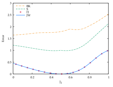
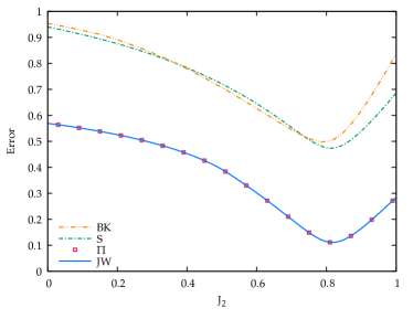
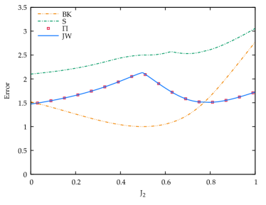
Figure 2: HFBF mean-field energy errors relative to the exact diagonalizations in the fermionized $2\times 4$ $J_{1}\text{--}J_{2}$ model with $J_{1}=1$ and either open boundary conditions (OBC) or periodic boundary conditions (PBC). Top left: $2\times 4$ labeling with OBC. Top right: $2\times 4$ labeling with PBC. Bottom left: $4\times 2$ labeling with OBC. Bottom right: $4\times 2$ labeling with PBC.

In this work, we will consider three $\mathfrak{su}(2)$ Hamiltonians: the $J_{1}\text{--}J_{2}$ Heisenberg model, the spin XXZ model, and the pairing Hamiltonian which we write in terms of spin operators. We will discuss results for each in turn. All of these Hamiltonians have $S_{z}$ symmetry, and we will always work in the $S_{z}=0$ sector for simplicity. In the parameter regimes we will consider, this is always the global ground state. In the thermodynamic limit, these Hamiltonians exhibit phase transitions which are of course absent in the exact solution for the finite systems we will consider here. Nevertheless, the presence of these multiple spin arrangements is reflected in mean-field solutions which frequently just cross one another. This leads to error curves which are not entirely smooth, because we have plotted, at each Hamiltonian parameter value, the lowest energy mean-field solution we could find.

Because our results depend on the labeling scheme chosen, we must say a bit about this first. In one dimension, we use the natural labeling scheme where sites connected in the lattice have sequential numbers, e.g., site 1 connects to site 2, site 2 to site 3, and so on. For the quasi-1D spin ladders, however, we have a “$2\times n$” labeling scheme and a “$n\times 2$” labeling scheme, depicted in Fig. 1. Put simply, the first number (“2” or “$n$”) denotes the faster-moving index in the 2D lattice.

IV.1 The $\boldsymbol{J_{1}}\text{--}\boldsymbol{J_{2}}$ Hamiltonian

The $J_{1}\text{--}J_{2}$ model has both nearest-neighbor and next-nearest neighbor interactions:

$$H_{J_{1}\text{--}J_{2}}=J_{1}\sum_{\langle pq\rangle}\vec{S}_{p}\cdot\vec{S}_{q}+J_{2}\,\sum_{\langle\langle pq\rangle\rangle}\vec{S}_{p}\cdot\vec{S}_{q},$$ (35)

where $\langle pq\rangle$ denotes nearest neighbors (sites connected in the lattice) and $\langle\langle pq\rangle\rangle$ denotes next-nearest neighbors. The physics is driven by the ratio $J_{2}/J_{1}$, where we will take both to be positive. For the 2D square lattice in the thermodynamic limit, the ground state is a Néel antiferromagnet for $J_{2}\lesssim 0.4\,J_{1}$ and a striped antiferromagnet for $J_{2}\gtrsim 0.6\,J_{1}$. In between, the magnetic structure is more complicated [42, 43, 44]. In this work we will focus on the quasi-1D spin ladders, i.e., $2\times n$ systems.

Figure 2 shows a comparison of the total energy errors with respect to the exact diagonalizations, resulting from the mean-field solutions with the four different fermionization schemes, both for open boundary conditions (OBC) and periodic boundary conditions (PBC), with $J_{1}=1$. As we have shown elsewhere [12, 13], resultings using mean-field theory in combination with the JW transformation are not quantitative but are greatly superior to what one obtains with an $\mathfrak{su}(2)$ mean-field technique. We can immediately see that the JW and $\Pi$ transformations give completely identical mean-field energies, which is sensible since, as we have noted, these two transformations are loosely speaking dual companions of one another. More formally, as we will discuss in future publications, the JW-transformed fermionic operators of Eqn. 15 and the $\Pi_{R}$-transformed operators of Eqn. 19 are, themselves, related by a mean-field canonical transformation of a form equivalent to HFBF; accordingly, the two seemingly different Hamiltonians have identical mean-field solutions.

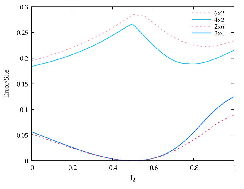
Figure 3: HFBF mean-field energy errors per site relative to the exact diagonalization in the $2\times 4$ and $2\times 6$ JW-transformed $J_{1}\text{--}J_{2}$ Hamiltonian.

The BK and Sierpinski mappings generally yield significantly worse mean-field results than do the other transformations we have considered. Mappings designed to minimize gate depth when mapping fermions to spins are not, evidently, the same as mappings designed to yield optimal mean-field solutions when mapping spins to fermions. The one apparent exception is in the $4\times 2$ case with PBC, where the BK mapping is, overall, superior in the physically interesting regime around $J_{2}=1/2$.

We also see the expected dependence on the labeling scheme, which we recall can be eliminated in the JW case (and, presumably, in the $\Pi$ case) by generalizing the strings $\tilde{\phi}_{p}$. It is interesting to note that we generally obtain superior results for OBC with the $4\times 2$ labeling and for PBC with the $2\times 4$ labeling where JW and $\Pi$ are exact at $J_{2}=1/2$, presumably related to the Majumdar–Ghosh point in the 1D $J_{1}\text{--}J_{2}$ model where the ground state at $J_{2}=1/2$ is exactly dimerized [45].

Finally, we compare results for the $2\times 4$ and $2\times 6$ models in Fig. 3. These results (consistent with those of Ref. 13) suggest that increasing system size does not necessarily degrade the quality of the mean-field results.

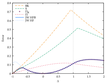
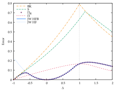
Figure 4: HFBF (BK, Sierpinski, $\Pi_{R}$, $\Pi$) and HF and HFB (JW) mean-field energy errors relative to the exact diagonalizations in the fermionized 8-site 1D XXZ model. Left panel: OBC. Right panel: PBC.

IV.2 The XXZ Hamiltonian

The XXZ Hamiltonian is also a spin lattice model, this time given by

$$H_{\mathrm{XXZ}}=\sum_{\langle pq\rangle}\left(S_{p}^{x}\,S_{q}^{x}+S_{p}^{y}\,S_{q}^{z}+\Delta\,S_{p}^{z}\,S_{q}^{z}\right).$$ (36)

Where the physics of the $J_{1}\text{--}J_{2}$ model depends on $J_{2}/J_{1}$, here it depends on $\Delta$. In one dimension, at $\Delta=0$ the JW-transformed XXZ model is exactly solved by HF with sites labeled in a natural sequential way. This is not the case in two or more dimensions, so we will consider both the 1D system and the 2D rectangular lattice. The point at $\Delta=1$ is the Heisenberg point, at which the Hamiltonian has $S^{2}$ symmetry, while $\Delta=-1$ is also a special point in which the exact ground state is given by the extreme antisymmetrized geminal power [46, 47].

The ground state over all $S_{z}$ sectors occurs at $S_{z}=0$ for $\Delta>-1$, while the different $S_{z}$ sectors are all degenerate with one another at $\Delta=-1$ and the global minimum of the energy occurs at maximal $S_{z}$ for $\Delta<-1$. Since we are focusing on $S_{z}=0$ we will only consider $\Delta\geq-1$ in this work. In the thermodynamic limit, for rectangular lattices, there is a phase transition at $\Delta=1$, where for $\Delta>1$ the ground state is antiferromagnetic with magnetization along the $z$ axis and for $|\Delta|<1$ the ground state is instead magnetized in the $xy$ plane [48].

We begin with the 1D case, depicted in Fig. 4, in which the JW strings do not contribute. Again, the $\Pi$ and JW transformations provide uniformly more accurate results than we obtain with the other two mappings considered, although all methods are exact at $\Delta=-1$ where, as we have indicated, the ground state energy for each $S_{z}$ sector is the same and spin mean field is already exact. As expected, we get the exact result at $\Delta=0$ with the JW transformation.

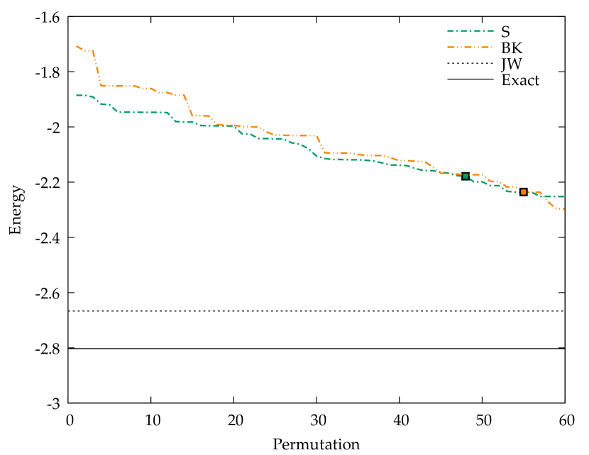
Figure 5: HFBF mean-field energy for the unique labelings of the 6-site 1D XXZ model at $\Delta=1$ with PBC, based on the BK and Sierpinski encodings. The lines marked “JW” and “Exact” denote, respectively, the energy of the mean-field solution based on the JW transformation with the natural labeling scheme 1-2-3-4-5-6, and the exact ground state energy. The squares indicate the result based on the natural labeling scheme.

Unlike with the $J_{1}\text{--}J_{2}$ model, the JW and $\Pi$ transformations do not generally give the same result, except at $\Delta=\pm 1$. At $\Delta=1$ the XXZ model is isotropic, but elsewhere it treats the $z$ component of spin differently from the other two. For this reason, we also show the $\Pi_{R}$ transformation which, like JW and like the Hamiltonian, treats the $z$ component of spin differently (because it does not include the string operator $\tilde{\phi}_{p}$). Indeed, the $\Pi_{R}$ transformation yields results completely equivalent to those we obtain with JW. We have also verified that a rotated JW transformation which has strings for the $y$ and $z$ spin components but not the $x$ component yields results identical to the original $\Pi$ transformation (data not shown).

We must mention one other consideration. For most $\Delta$ values, the fermionic mean-field for the JW-transformed Hamiltonian is HF. Near $\Delta=-1$, however, number symmetry breaks spontaneously and we can distinguish HF and HFB solutions. Where these two methods differ, it is the lower energy of the two (the HFB) with which the HFBF solution for the $\Pi_{R}$ transformation agrees.

One may wonder whether the poor performance of the BK or Sierpinski encodings in this context is simply due to having chosen the wrong labeling scheme. We have seen that labeling schemes matter for all of these encodings, and previous work has found that the natural labeling scheme we have chosen is, on the whole, the best available for the 1D XXZ model with the JW transformation. But is that the case for these encodings?

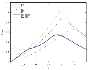
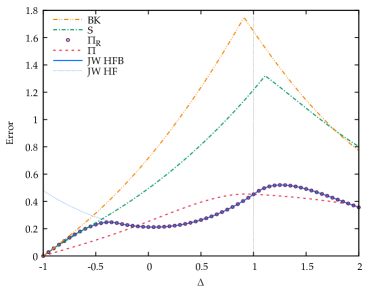
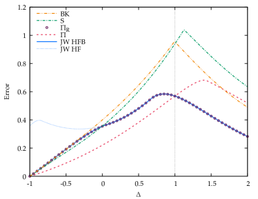
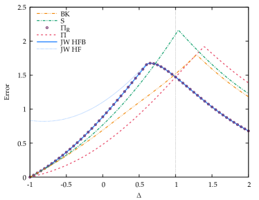
Figure 6: HFBF (BK, Sierpinski, $\Pi_{R}$, $\Pi$) and HF and HFB (JW) mean-field energy errors relative to the exact diagonalizations in the fermionized $2\times 4$ XXZ model with either open boundary conditions (OBC) or periodic boundary conditions (PBC). Top left: $2\times 4$ labeling with OBC. Top right: $2\times 4$ labeling with PBC. Bottom left: $4\times 2$ labeling with OBC. Bottom right: $4\times 2$ labeling with PBC.

To answer that question, we have looked at the 6-site 1D XXZ model with PBC. Here, there are 60 distinct labeling schemes ($6!$ ways of labeling the sites, reduced by a factor of 6 due to translational symmetry and by another factor of 2 due to reflection symmetry) and we have tried the BK and Sierpinski encodings at $\Delta=1$ for all 60 distinct labelings. The results in Fig. 5 make clear that no relabeling of the sites will suffice to remedy the poor performance of mean-field methods based on these encodings, at least at $\Delta=1$ but presumably also for other values of $\Delta$.

Results for the 2D XXZ model are roughly similar to those for the 1D case (see Fig. 6) although the mean-field methods are generally less accurate. For the JW and $\Pi$ transformations, this is presumably because the strings $\tilde{\phi}_{p}$ which vanished in 1D now contribute in 2D. The BK and Sierpinski encodings are more competitive with the JW and $\Pi$ encodings in this quasi-1D case than they are in the genuinely 1D case, but the JW and $\Pi$ encodings still generally appear to yield superior mean-field results.

IV.3 The Pairing Hamiltonian

The pairing Hamiltonian, also known as the reduced Bardeen–Cooper–Schrieffer Hamiltonian, is not really a Hamiltonian of spins at all. Instead, it is a Hamiltonian consisting of electron pair creation, pair annihilation, and number operators. As these operators satisfy the same $\mathfrak{su}(2)$ algebra as do the spin operators, however, we can write the pairing model as a spin Hamiltonian, in which case it takes the form

$$H_{P}=\sum_{p}\epsilon_{p}\,\left(2\,S_{p}^{z}-1\right)-G\,\sum_{pq}S_{p}^{+}\,S_{q}^{+}.$$ (37)

This Hamiltonian is exactly solvable with a form of Bethe ansatz [49, 50, 51], for any choice of $\epsilon_{p}$ and $G$.

We can eliminate the $p=q$ term in the interaction, using $S_{p}^{+}\,S_{p}^{-}=\frac{1}{2}+S_{p}^{z}$, thereby absorbing this diagonal contribution into the first, Zeeman-like, term. As a practical matter, we choose to work at half filling, in which case we can rewrite the Hamiltonian as

$$H_{P}^{\prime}=2\,\sum_{p}\epsilon_{p}\,S_{p}^{z}-G\,\sum_{p\neq q}S_{p}^{+}\,S_{q}^{+}=H_{P}-\lambda\,S_{z}$$ (38)

and pick the $\epsilon$ to be equally spaced and centered around 0. The chemical potential $\lambda$ enforces that the ground state is $S_{z}=0$ everywhere, and the physics is driven by the parameter $G$.

If we disregard the chemical potential for a moment and consider only the first form of the Hamiltonian, we can see that as $|G|$ tends to $\infty$, so that the Zeeman-like term is irrelevant, then

$$\frac{1}{|G|}\,H_{P}\to\mp\,S_{+}\,S_{-}=\mp\left(S^{2}-S_{z}^{2}+S_{z}\right),$$ (39)

where $S_{+}=\sum_{p}S_{p}^{+}$ and similarly for $S_{-}$ and $S_{z}$; the sign is $\mp$ as $G\to\pm\infty$. Accordingly, the $S_{z}=0$ ground state occurs for maximal $S^{2}$ in the $G\to\infty$ limit and for $S^{2}=0$ in the $G\to-\infty$ limit. Respectively, these amount to an extreme form of the antisymmetrized geminal power, and a kind of dimerized state obtained by taking one of the (many) degenerate $S^{2}=0$ states. See Refs. 52, 53, 54 for details.

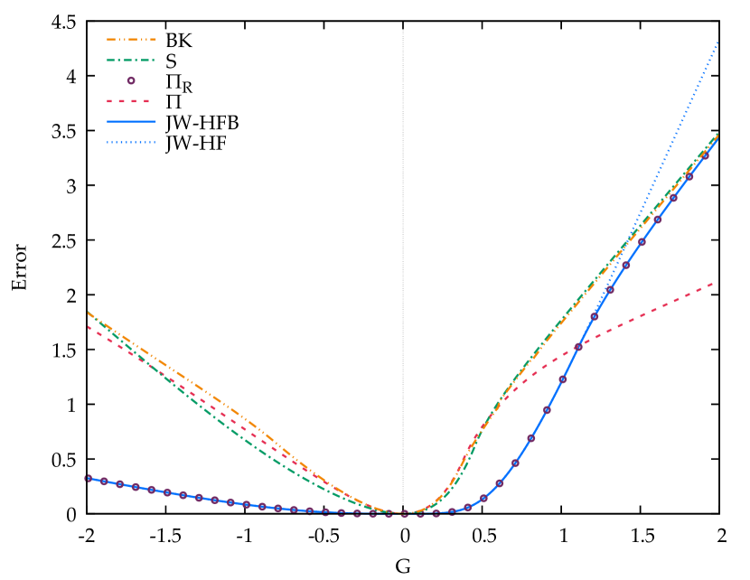
Figure 7: HFBF (BK, Sierpinski, $\Pi_{R}$, $\Pi$) and HF and HFB (JW) mean-field energy errors relative to the exact diagonalizations in the fermionized 8-site pairing model.

The pairing model presents a particular challenge. Where in the 2D XXZ models, each spin interacted with at most three other spins, in the pairing model, each spin interacts equivalently with every other spin. Indeed, Fig. 7 shows that for the pairing model, our results are generally rather poor away from $G=0$, though again the JW and (rotated) $\Pi$ transformations are superior to the other fermionizations on the repulsive side ($G<0$).

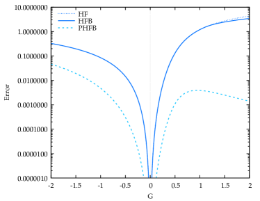
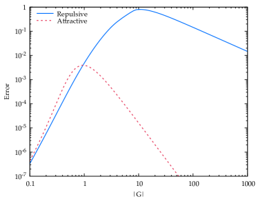
Figure 8: Mean-field energy errors relative to the exact diagonalizations in the 8-site pairing model transformed with JW. Left panel: Comparison between HF, HFB, and PHFB. Right panel: PHFB errors on a log-log scale to show the large $|G|$ behavior.

IV.4 Fermionic Number Projection

For most of these fermionizations, we have gone about as far as we can go with mean-field theory. For the JW transformation, however, we can do a bit better. This is because the JW transformation maps the global $S_{z}$ symmetry of the $\mathfrak{su}(2)$ Hamiltonian to global number symmetry of the fermionic Hamiltonian, and we can deliberately break and then projectively restore this number symmetry to do a JW-transformed number-projected HFB. For details about number projection, see Refs. 55, 56, 57, but the gist is that we write the projected HFB (PHFB) wave function as an HFB state and then project out those components with the incorrect particle number. We could do something analagous for any of the other encodings – the global $S_{z}$ symmetry maps under all of them to some symmetry of the fermionic Hamiltonian – but JW has the advantage that this symmetry is both obvious and, more importantly, given by a one-body operator. As such, the projection can be efficiently implemented in a self-consistent field code.

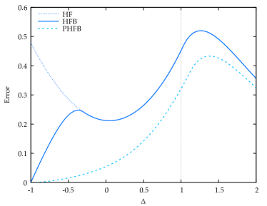
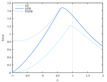
Figure 9: Energy errors relative to the exact diagonalizations in the $2\times 4$ JW-transformed XXZ model with PBC for HF, HFB, and PHFB. Left panel: $2\times 4$ labeling. Right panel: $4\times 2$ labeling.

Fortunately, PHFB provides quite reasonable accuracy for the JW-transformed pairing Hamiltonian, as seen in Fig. 8. In fact, it is energetically exact in both the strongly attractive ($G\to\infty$) and strongly repulsive ($G\to-\infty$) limits. We prove this in the appendix.

Figure 9 shows that PHFB is also a useful improvement upon HF or HFB in the JW-transformed XXZ model. Indeed, PHFB is variationally bounded from above by HFB (at least when we are looking at the ground state number sector), so it must be at least as good as the results we obtained for the $J_{1}\text{--}J_{2}$ and XXZ models with HFB on the JW-transformed Hamiltonian.

V Discussion

Each of the fermionizations we have considered preserves the exact spectrum of the spin Hamiltonian, but they generally give different results at the mean-field level. In other words, all fermionizations are equivalent in the full Fock space, but some fermionizations are more compatible with mean-field approaches than others. For the Hamiltonians we have considered, those fermion to $\mathfrak{su}(2)$ mappings designed to produce more efficient encodings seem to yield fermionic Hamiltonians whose mean-field solutions are energetically less accurate. This is so even though the JW or $\Pi$ transformations involve the very nonlocal JW strings $\tilde{\phi}_{p}$, which the BK and Sierpinski encodings eliminate. Fortunately, the action of the JW string on a fermionic mean-field state is to produce another mean-field state by virtue of the Thouless theorem [36]. This means that it is actually straightforward to account for the JW strings when evaluating matrix elements, by simply using the non-orthogonal Wick’s theorem [40], though some care must be taken to implement this idea in a numerically robust and efficient way [41].

Another advantage of the JW transformation is that by generalizing the string from $\tilde{\phi_{p}}=\exp(\mathrm{i}\,\pi\,\sum_{q<p}n_{q})$ to

$$\hat{\phi}_{p}=\mathrm{e}^{\mathrm{i}\,\sum_{q}\theta_{qp}\,n_{q}}\,\tilde{\phi}_{p}$$ (40)

where the matrix of parameters $\boldsymbol{\theta}$ is symmetric with vanishing diagonals, we can obtain results invariant to the labeling of the spin lattice [13] when $\boldsymbol{\theta}$ is optimized. This generalization, too, can be readily implemented using nonorthogonal Wick’s theorem. The same should be true for the $\Pi$ transformation.

There is one additional advantage which suggests we should prefer to use the JW transformation to the $\Pi$ mapping: the JW mapping converts an $\mathfrak{su}(2)$ Hamiltonian with $S_{z}$ symmetry to a fermionic Hamiltonian with number symmetry. This permits us to select several different levels of mean-field theory: HF, HFB, HFBF, as well as their number-projected counterparts. The other mappings all require us to use the rather more complicated HFBF mean-field theory or to employ Colpa’s trick to replace HFBF for $M$ fermions with HFB for $M+1$ fermions (and the latter is pragmatically simpler) and generally do not permit symmetry projection at all. This is not to say that these fermionized Hamiltonians do not inherit the symmetries of the underlying spin Hamiltonian, because naturally they do. Rather, these symmetries are not generally one-body symmetries and therefore are difficult to project efficiently.

For all of these reasons, it seems clear that the JW transformation, in addition to being the oldest mapping relating spins to fermions, is (in the context of mapping spin Hamiltonians to fermions for mean-field solution) also the most powerful (at least among those we have tried).

VI Data Availability

The data that support the findings of this study are available from the corresponding author upon reasonable request.

Appendix A Exactness of JW-PHFB for the Pairing Model

Here we demonstrate exactness of number-projected HFB in the $G\to\pm\infty$ limit of the JW–transformed pairing model. As we have noted, in the $S_{z}=0$ sector we can work with the simpler Hamiltonian

$$H_{\mathrm{eff}}=\mp S^{2};$$ (41)

see Eqn. 39.

Let us start with the attractive limit. In this case, we know that the ground state we seek has $S_{z}=0$ and maximal $S^{2}$. We can build this by starting with the state with all spins $\downarrow$ and applying the global raising operator the appropriate number of times to reach

$$\ket{\Psi_{A}}=\frac{1}{N!}\,\left(\sum_{p}S_{p}^{+}\right)^{N}\ket{\Downarrow}=P_{S_{z}}\,\mathrm{e}^{\sum_{p}S_{p}^{+}}\ket{\Downarrow}$$ (42)

where $N$ is the number of $\uparrow$ spins and $\ket{\Downarrow}$ is the vacuum in which each spin is $\downarrow$; $P_{S_{z}}$ is the projector onto the appropriate $S_{z}$ sector. The wave function $\exp(\sum_{p}S_{p}^{+})\ket{\Downarrow}$ is a spin mean-field state.

Now transform this wave function with the JW transformation. Because $S_{z}$ becomes particle number, $P_{S_{z}}$ transforms to the fermionic number projector. We have argued elsewhere [32] (and prove in the supplementary material) that a spin mean-field state maps into a fermionic HFBF state, which means that $\ket{\Psi_{A}}$ maps, under JW transformation, into a number-projected HFBF state. But a number-projected HFBF state is also a number-projected HFB state since HFBF is just a linear combination of an even-particle number HFB and an odd-particle number HFB. Ergo, the exact ground state in the $G\to\infty$ limit of the pairing model maps, under JW, into PHFB.

The repulsive limit is more complicated. As we have noted, it is an $S^{2}=0$ state, which we can get by the standard machinery of coupling angular momenta. One way to write (one of) the ground states is in a dimerized form:

$$\ket{\Psi_{R}} =\ket{s_{12}}\otimes\ket{s_{34}}\ldots\ket{s_{M-1,M}},$$ (43a)

$$\ket{s_{pq}} =\ket{\uparrow_{p}\downarrow_{q}}-\ket{\downarrow_{p}\uparrow_{q}},$$ (43b)

where we have a total of $M$ spins. That is, we divide the system into disjoint pairs and place each pair in a separate singlet state. We can express this wave function as

$$\ket{\Psi_{R}}=\left[\prod_{k=1}^{M/2}\left(1-S_{2k}^{+}\,S_{2k-1}^{-}\right)\right]\ket{\uparrow\downarrow\uparrow\downarrow\ldots}.$$ (44)

Now we transform the wave function with the JW transformation. The state $\ket{\uparrow\downarrow\uparrow\downarrow\ldots}$ becomes a fermionic state $\ket{1010\ldots}$ with odd levels occupied and even levels empty. The operator $S_{2k}^{+}\,S_{2k-1}^{-}$ transforms as

$$S_{2k}^{+}\,S_{2k-1}^{-} \underset{\text{JW}}{\mapsto}c_{2k}^{\dagger}\,\tilde{\phi}_{2k}\,\tilde{\phi}_{2k-1}\,c_{2k-1}$$ (45a)

$$=c_{2k}^{\dagger}\,c_{2k-1}$$ (45b)

where we have used that $\tilde{\phi}_{2k}\,\tilde{\phi}_{2k+1}=1-2\,c^{\dagger}_{2k-1}\,c_{2k-1}$ so that JW strings between sequential fermionic operators cancel out.

All of this means that

$$\ket{\Psi_{R}} \underset{\text{JW}}{\mapsto}\left[\prod_{k=1}^{M/2}\left(1-c_{2k}^{\dagger}\,c_{2k-1}\right)\right]]\ket{1010\ldots}$$ (46a)

$$=\left[\prod_{k=1}^{M/2}\mathrm{e}^{-c_{2k}^{\dagger}\,c_{2k-1}}\right]\ket{1010\ldots}$$ (46b)

$$=\mathrm{e}^{-\sum_{k=1}^{M/2}c_{2k}^{\dagger}\,c_{2k-1}}\ket{1010\ldots},$$ (46c)

which is the Thouless representation of an HF state. Thus, HF is already energetically exact in the $G\to-\infty$ limit of the JW–transformed pairing Hamiltonian, and as HF is a special case of PHFB, this means PHFB is also energetically exact.

Appendix B The 8-Site Bravyi-Kitaev and Sierpinski Transformations

For the JW and $\Pi$ transformations, it is straightforward to write down both the mapping from fermions to spins and the inverse mapping from spins back to fermions. For the BK and Sierpinski mappings, this is less easy. Accordingly, we note the 8-site mappings we have used here. More specifically, we record the mappings from the Pauli operators $\sigma^{x}$ and $\sigma^{z}$ to the Majoranas; we extract $\sigma^{y}$ from

$$\sigma_{p}^{z}\,\sigma_{p}^{x}=\mathrm{i}\,\sigma_{p}^{y}.$$ (47)

For brevity we define the Majorana products

$$A_{p} =\mathrm{i}\,\gamma_{1,p}\,\gamma_{2,p}=1-2\,c_{p}^{\dagger}\,c_{p},$$ (48a)

$$B_{p} =\mathrm{i}\,\gamma_{2,p}\,\gamma_{1,p+1}.$$ (48b)

These objects are Hermitian, mutually commuting, and satisfy $A_{p}^{2}=B_{p}^{2}=1$. They also commute with individual Majorana operators, except that they anticommute with their constitutents, i.e., $A_{p}$ anticommutes with $\gamma_{1,p}$ and $\gamma_{2,p}$ while $B_{p}$ anticommutes with $\gamma_{1,p+1}$ and $\gamma_{2,p}$.

The 8-site BK spin-to-fermion mapping is

$$\sigma_{1}^{x} \underset{\text{BK}}{\mapsto}B_{1}\qquad \sigma_{1}^{z} \underset{\text{BK}}{\mapsto}A_{1},$$ (49a)

$$\sigma_{2}^{x} \underset{\text{BK}}{\mapsto}B_{2}\,B_{3}\qquad \sigma_{2}^{z} \underset{\text{BK}}{\mapsto}A_{1}\,A_{2},$$ (49b)

$$\sigma_{3}^{x} \underset{\text{BK}}{\mapsto}B_{3}\qquad \sigma_{3}^{z} \underset{\text{BK}}{\mapsto}A_{3},$$ (49c)

$$\sigma_{4}^{x} \underset{\text{BK}}{\mapsto}B_{4}\,B_{5}\,B_{6}\,B_{7}\qquad \sigma_{4}^{z} \underset{\text{BK}}{\mapsto}A_{1}\,A_{2}\,A_{3}\,A_{4},$$ (49d)

$$\sigma_{5}^{x} \underset{\text{BK}}{\mapsto}B_{5}\qquad \sigma_{5}^{z} \underset{\text{BK}}{\mapsto}A_{5},$$ (49e)

$$\sigma_{6}^{x} \underset{\text{BK}}{\mapsto}B_{6}\,B_{7}\qquad \sigma_{6}^{z} \underset{\text{BK}}{\mapsto}A_{5}\,A_{6},$$ (49f)

$$\sigma_{7}^{x} \underset{\text{BK}}{\mapsto}B_{7}\qquad \sigma_{7}^{z} \underset{\text{BK}}{\mapsto}A_{7},$$ (49g)

$$\sigma_{8}^{x} \underset{\text{BK}}{\mapsto}-\mathrm{i}\,\Pi\,\gamma_{2,8}\qquad \sigma_{8}^{z} \underset{\text{BK}}{\mapsto}\Pi,$$ (49h)

while the 8-site Sierpinski spin-to-fermion mapping is instead

$$\sigma^{x}_{1} \underset{\text{S}}{\mapsto}B_{1}\qquad \sigma^{z}_{1} \underset{\text{S}}{\mapsto}A_{1},$$ (50a)

$$\sigma^{x}_{2} \underset{\text{S}}{\mapsto}B_{2}\,B_{3}\,B_{4}\qquad \sigma^{z}_{2} \underset{\text{S}}{\mapsto}A_{1}\,A_{2}\,A_{3},$$ (50b)

$$\sigma^{x}_{3} \underset{\text{S}}{\mapsto}B_{2}\qquad \sigma^{z}_{3} \underset{\text{S}}{\mapsto}A_{3},$$ (50c)

$$\sigma^{x}_{4} \underset{\text{S}}{\mapsto}B_{4}\qquad \sigma^{z}_{4} \underset{\text{S}}{\mapsto}A_{4},$$ (50d)

$$\sigma^{x}_{5} \underset{\text{S}}{\mapsto}B_{1}\,B_{2}\,B_{3}\,B_{4}\,\gamma_{1,1}\qquad \sigma^{z}_{5} \underset{\text{S}}{\mapsto}\Pi\,A_{7}\,A_{8},$$ (50e)

$$\sigma^{x}_{6} \underset{\text{S}}{\mapsto}B_{5}\qquad \sigma^{z}_{6} \underset{\text{S}}{\mapsto}A_{6},$$ (50f)

$$\sigma^{x}_{7} \underset{\text{S}}{\mapsto}B_{7}\qquad \sigma^{z}_{7} \underset{\text{S}}{\mapsto}A_{7},$$ (50g)

$$\sigma^{x}_{8} \underset{\text{S}}{\mapsto}\mathrm{i}\,\Pi\,\gamma_{2,8}\qquad \sigma^{z}_{8} \underset{\text{S}}{\mapsto}A_{7}\,A_{8}.$$ (50h)

Overall signs are arbitrary, but factors of $\mathrm{i}$ are not. Ultimately, this is because we can multiply any two Paulis by $-1$ without changing the $\mathfrak{su}(2)$ commutation rules.

Recall that $\Pi$ is the number parity operator (c.f. Eqn. (18b)), given in this notation as

$$\Pi=\prod_{p}A_{p}.$$ (51)

References

- Batista and Ortiz [2001] C. D. Batista and G. Ortiz, in Condensed Matter Theories, Vol. 16, edited by S. Hernandez and W. J. Clark (Nova Science Publishers, Inc, Huntington, New York, 2001) pp. 1–15.
- Nishimori and Ortiz [2011] H. Nishimori and G. Ortiz, Elements of Phase Transitions and Critical Phenomena (Oxford University Press, Oxford, 2011) p. 220.
- Jordan and Wigner [1928] P. Jordan and E. Wigner, Zeitschrift für Physik 47, 631 (1928).
- Gonçalves et al. [2005] L. L. Gonçalves, L. P. S. Coutinho, and J. P. de Lima, Physica A 345, 71 (2005).
- Verkholyak et al. [2006] T. Verkholyak, A. Honecker, and W. Brenig, Eur. Phys. J. B 49, 283 (2006).
- Kitaev and Laumann [2008] A. Kitaev and C. Laumann, Topological phases and quantum computation, Lectures given by Alexei Kitaev at the 2008 Les Houches summer school “Exact methods in low-dimensional physics and quantum computing.” (2008).
- Verkholyak et al. [2010] T. Verkholyak, J. Strečka, M. Jaščur, and J. Richter, Acta Phys. Pol. A 118, 978 (2010).
- Bardyn and İmamoǧlu [2012] C.-E. Bardyn and A. İmamoǧlu, Phys. Rev. Lett. 109, 253606 (2012).
- Zvyagin [2013] A. A. Zvyagin, Phs. Rev. Lett. 110, 217207 (2013).
- Greiter et al. [2014] M. Greiter, V. Schnells, and R. Thomale, Ann. Phys. 351, 1026 (2014).
- Gebhard et al. [2022] F. Gebhard, K. Bauerbach, and Ö. Legeza, Phys. Rev. B 106, 205133 (2022).
- Henderson et al. [2022] T. M. Henderson, G. P. Chen, and G. E. Scuseria, J. Chem. Phys. 157, 194114 (2022).
- Henderson et al. [2024a] T. M. Henderson, F. Gao, and G. E. Scuseria, Mol. Phys. 122, e2254857 (2024a).
- Bravyi and Kitaev [2002] S. B. Bravyi and A. Y. Kitaev, Ann. Phys. 298, 210 (2002).
- Cao et al. [2019] Y. Cao, J. Romero, J. P. Olson, M. Degroote, P. D. Johnson, M. Kieferová, I. D. Kivlichan, T. Menke, B. Peropadre, N. P. D. Sawaya, S. Sim, L. Veis, and A. Aspuru-Guzik, Chem. Rev. 119, 10856 (2019).
- Bauer et al. [2020] B. Bauer, S. Bravyi, M. Mottao, and G. K. Chan, Chem. Rev. 120, 12685 (2020).
- McArdle et al. [2020] S. McArdle, S. Endo, A. Aspuru-Guzik, S. C. Benjamin, and X. Yuan, Rev. Mod. Phys. 92, 015003 (2020).
- Verstraete and Cirac [2005] F. Verstraete and J. I. Cirac, J. Stat. Mech. 2005, P09012 (2005).
- Seeley et al. [2012] J. T. Seeley, M. J. Richard, and P. J. Love, J. Chem. Phys. 137, 224109 (2012).
- Havlíček et al. [2017] V. Havlíček, M. Troyer, and J. D. Whitfield, Phys. Rev. A 95, 032332 (2017).
- Bravyi et al. [2017] S. Bravyi, J. M. Gambetta, A. Mezzacapo, and K. Temme, Tapering off qubits to simulate fermionic hamiltonians (2017), arXiv:1701.08213 [quant-ph] .
- Setia et al. [2019] K. Setia, S. Bravyi, A. Mezzacapo, and J. D. Whitfield, Phys. Rev. Res. 1, 033033 (2019).
- Jiang et al. [2020] Z. Jiang, A. Kalev, W. Mruczkiewicz, and H. Neven, Quantum 4, 276 (2020).
- Picozzi and Tennyson [2023] D. Picozzi and J. Tennyson, Quantum Sci. Technol. 8, 035026 (2023).
- Liu et al. [2024] Y. Liu, S. Che, J. Zhou, Y. Shi, and G. Li, in ASPLOS 2024 (2024).
- Harrison et al. [2023] B. Harrison, D. Nelson, D. Adamiak, and J. Whitfield, Reducing the qubit requirement of Jordan-Wigner encodings of -mode, -fermion systems from to (2023), arXiv:2211.04501 [quant-ph] .
- O’Brien and Strelchuk [2024] O. O’Brien and S. Strelchuk, Phys. Rev. B 109, 115149 (2024).
- Harrison et al. [2024] B. Harrison, M. Chiew, J. Necaise, A. Projansky, S. Strelchuk, and J. D. Whitfield, A Sierpinski triangle fermion-to-qubit transform (2024), arXiv:2409.04348 [quant-ph] .
- Fukutome et al. [1977] H. Fukutome, M. Yamamura, and S. Nishiyama, Prog. Theor. Phys. 57, 1554 (1977).
- Fukutome [1977] H. Fukutome, Prog. Theor. Phys. 58, 1692 (1977).
- Moussa [2012] J. E. Moussa, Generalized unitary Bogoliubov transformation that breaks fermion number parity (2012), arXiv:1208.1086 [cond-mat.str-el] .
- Henderson et al. [2024b] T. M. Henderson, S. Ghassemi Tabrizi, G. P. Chen, and G. E. Scuseria, J. Chem. Phys. 160, 064103 (2024b).
- Chiew and Strelchuk [2023] M. Chiew and S. Strelchuk, Quantum 7, 1145 (2023).
- Wang [1991] Y. R. Wang, Phys. Rev. B 43, 3786 (1991).
- Tranter et al. [2015] A. Tranter, S. Sofia, J. Seeley, M. Kaicher, J. McClean, R. Babbush, P. V. Coveney, F. Mintert, F. Wilhelm, and P. J. Love, International Journal of Quantum Chemistry 115, 1431 (2015), https://onlinelibrary.wiley.com/doi/pdf/10.1002/qua.24969 .
- Thouless [1960] D. J. Thouless, Nucl. Phys. 21, 225 (1960).
- Bach et al. [1994] V. Bach, E. H. Lieb, and J. P. Solovej, J. Stat. Phys. 76, 3 (1994).
- Colpa [1979] J. H. P. Colpa, J. Phys. A: Math. Gen. 12, 49 (1979).
- Nishiyama and da Providência [2019] S. Nishiyama and J. da Providência, Internat. J. Geom. Meth. in Mod. Phys. 16, 1950184 (2019).
- Balian and Brezin [1969] R. Balian and E. Brezin, Il Nuovo Cimento B 64, 37 (1969).
- Chen and Scuseria [2023] G. P. Chen and G. E. Scuseria, J. Chem. Phys. 158, 231102 (2023).
- Darradi et al. [2008] R. Darradi, O. Derzhko, R. Zinke, J. Schulenburg, S. E. Krüger, and J. Richter, Phys. Rev. B 78, 214415 (2008).
- Gong et al. [2014] S.-S. Gong, W. Zhu, D. N. Sheng, O. I. Motrunich, and M. P. A. Fisher, Phys. Rev. Lett. 113, 027201 (2014).
- Richter et al. [2015] J. Richter, R. Zinke, and D. J. J. Farnell, Eur. Phys. J. B 88, 2 (2015).
- Majumdar and Ghosh [1969] C. Majumdar and D. K. Ghosh, J. Math. Phys. 10, 1388 (1969).
- Massaccesi et al. [2021] G. E. Massaccesi, A. Rubio-García, P. Capuzzi, E. Ríos, O. B. Oña, J. Dukelsky, L. Lain, A. Torre, and D. R. Alcoba, J. Stat. Mech. 2021, 013110 (2021).
- Liu et al. [2023] Z. Liu, F. Gao, G. P. Chen, T. M. Henderson, J. Dukelsky, and G. E. Scuseria, Phys. Rev. B 108, 085136 (2023).
- Farnell and Bishop [2004] D. J. J. Farnell and R. F. Bishop, The coupled cluster method applied to quantum magnetism, in Quantum Magnetism, edited by U. Schollwöck, J. Richter, D. J. J. Farnell, and R. F. Bishop (Springer, Berlin, Heidelberg, 2004) pp. 307–348.
- Richardson [1963] R. W. Richardson, Phys. Lett. 3, 277 (1963).
- Richardson and Sherman [1964] R. W. Richardson and N. Sherman, Nucl. Phys. 52, 221 (1964).
- Richardson [1965] R. W. Richardson, J. Math. Phys. 6, 1034 (1965).
- Yuzbashyan et al. [2003] E. A. Yuzbashyan, A. A. Baytin, and B. L. Altshuler, Phys. Rev. B 68, 214509 (2003).
- Faribault et al. [2010] A. Faribault, P. Calabrese, and J.-S. Caux, Phys. Rev. B 81, 174507 (2010).
- Johnson [2023] P. A. Johnson, Richardson-Gaudin States (2023), arXiv:2312.08804 [physics.chem-ph] .
- Sheikh and Ring [2000] J. A. Sheikh and P. Ring, Nucl. Phys. A 665, 71 (2000).
- Schmid [2004] K. Schmid, Prog. Part. Nucl. Phys. 52, 565 (2004).
- Scuseria et al. [2011] G. E. Scuseria, C. A. Jiménez-Hoyos, T. M. Henderson, K. Samanta, and J. K. Ellis, J. Chem. Phys. 135, 124108 (2011).