MixLinear: Extreme Low Resource Multivariate Time Series Forecasting with $0.1K$ Parameters

Abstract

Recently, there has been a growing interest in Long-term Time Series Forecasting (LTSF), which involves predicting long-term future values by analyzing a large amount of historical time-series data to identify patterns and trends. There exist significant challenges in LTSF due to its complex temporal dependencies and high computational demands. Although Transformer-based models offer high forecasting accuracy, they are often too compute-intensive to be deployed on devices with hardware constraints. On the other hand, the linear models aim to reduce the computational overhead by employing either decomposition methods in the time domain or compact representations in the frequency domain. In this paper, we propose MixLinear, an ultra-lightweight multivariate time series forecasting model specifically designed for resource-constrained devices. MixLinear effectively captures both temporal and frequency domain features by modeling intra-segment and inter-segment variations in the time domain and extracting frequency variations from a low-dimensional latent space in the frequency domain. By reducing the parameter scale of a downsampled $n$-length input/output one-layer linear model from $O(n^{2})$ to $O(n)$, MixLinear achieves efficient computation without sacrificing accuracy. Extensive evaluations with four benchmark datasets show that MixLinear attains forecasting performance comparable to, or surpassing, state-of-the-art models with significantly fewer parameters ($0.1K$), which makes it well-suited for deployment on devices with limited computational capacity.

1 Introduction

Time-series modeling is crucial for various fields, including climate science (Moon & Wettlaufer, 2017), biological research (Watson et al., 2021), medicine (Kim et al., 2014), retail (Nunnari & Nunnari, 2017), and finance (Sezer et al., 2020). Accurate time series forecasting is essential for informed decision-making and strategic planning in these domains. Traditional approaches, such as Autoregressive (AR) models (Nassar et al., 2004), exponential smoothing (Gardner Jr, 1985), and structural time-series models (Harvey, 1990), have established a strong foundation for time-series forecasting. In recent years, there has been a growing interest in Long-term Time Series Forecasting (LTSF), which aims to predict long-term future values by identifying patterns and trends in large amounts of historical time-series data. Recent research has demonstrated that leveraging advanced machine learning techniques, such as Gradient Boosted Regression Trees (GBRT) (Mohan et al., 2011), and deep learning models, including Recurrent Neural Networks (RNN) (Salehinejad et al., 2017) and Temporal Convolutional Networks (TCN) (He & Zhao, 2019), yields significant performance improvements over traditional methods.

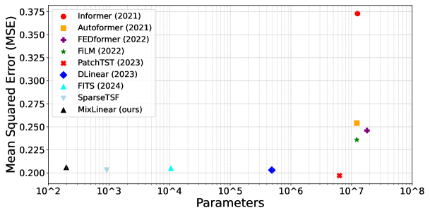
Figure 1: Comparison of MSE and parameters between MixLinear and other mainstream models of the Electricity dataset with a forecast horizon of $720$.

Over the last few years, significant efforts have been made to explore the use of Transformers for LTSF and produced many good models, such as LogTrans (Nie et al., 2022), Informer (Zhou et al., 2021), Autoformer (Wu et al., 2021), Pyraformer (Liu et al., 2021), Triformer (Cirstea et al., 2022), FEDformer (Zhou et al., 2022b), and PatchTST (Nie et al., 2023). Those models achieve good forecasting performance at the cost of introducing significant computation overhead due to the use of the self-attention mechanism, which scales quadratically with sequence length $L$. The high computational demands and large memory requirements of these models hinder their deployment for LTSF tasks on resource-constrained devices. To address this limitation and facilitate low-resource usage, researchers have proposed refined linear models based on decomposition techniques that achieve comparable performance with significantly fewer parameters. For instance, FITS (Xu et al., 2024) attains superior performance using interpolation in the complex frequency domain with only $10K$ parameters, while SparseTSF (Lin et al., 2024) further reduces the parameter count to $1K$ while maintaining robust performance.

However, current research in LTSF focuses on efficiently decomposing and capturing dependencies from either the time domain or frequency domain. For instance, Informer employs an attention-distilling method to reduce complexity (Zhou et al., 2021) in the time domain, PatchTST utilizes a patching technique to transform time series into subseries-level patches for increased efficiency (Nie et al., 2023), and SparseTSF simplifies forecasting by decoupling periodicity and trend (Lin et al., 2024). In the frequency domain, FEDformer decomposes sequences into multiple frequency domain modes using frequency transforms to extract features (Zhou et al., 2022b). TimesNet (Wu et al., 2022) employs a frequency-based method to separate intraperiod and interperiod variations. FITS utilizes a complex-valued neural network to capture both amplitude and phase information simultaneously, providing a more comprehensive and efficient approach to processing time series data (Xu et al., 2024).

In this paper, we introduce MixLinear a highly lightweight multivariate time series forecasting model, which efficiently captures the temporal and frequency features from both time and frequency domains. It captures intra-segment and inter-segment variations in the time domain by decoupling channel and periodic information from the trend components, breaking the trend information into smaller segments. In the frequency domain, it captures frequency domain variations by mapping the decoupled time series subsequences (trend) into a latent frequency space and reconstructing the trend spectrum. MixLinear reduces the parameter requirement from $O(n^{2})$ to $O(n)$ for $L$-length inputs/outputs with a known period $w$ and subsequence length $n=\left\lceil\frac{L}{w}\right\rceil$. Our comprehensive evaluation of LTSF with benchmark datasets shows that MixLinear provides comparable or better forecasting accuracy with much fewer parameters ($0.1K$) compared to state-of-the-art models. For instance, as Fig. 1 shows, MixLinear achieves a Mean Squared Error (MSE) of $0.208$ on the Electricity dataset with a forecast horizon of $720$ with $195$ parameters.

In summary, our contributions in the paper are as follows:

• We introduce an extremely lightweight model MixLinear that can achieve state-of-the-art comparable or better forecasting accuracy with only $0.1K$ parameters.

• To our knowledge, Mixlinear is the first lightweight LTSF model that captures temporal and frequency features from both time and frequency domains. MixLinear applies the trend segmentation in the time domain to capture the intra-segment and inter-segment variations. MixLinear captures amplitude and phase information by reconstructing the trend spectrum from low dimensional latent space in the frequency domain.

• To evaluate our model, we conduct experiments on several widely used LTSF benchmark datasets. MixLinear consistently delivers top-tier performance across a variety of time series tasks and achieves up to a $5.3\%$ reduction in MSE on these benchmarks.

2 Preliminaries

Long-term Time Series Forecasting.

The task of LTSF involves predicting future values over an extended horizon using previously observed multivariate time series data. It is formalized as $\hat{x}_{t+1:t+H}=f(x_{t-L+1:t})$, where $x_{t-L+1:t}\in\mathbb{R}^{L\times C}$ and $\hat{x}_{t+1:t+H}\in\mathbb{R}^{H\times C}$. In this formulation, $L$ denotes the length of the historical observation window, $C$ represents the number of distinct features or channels, and $H$ denotes the length of the forecast horizon. The main goal of LTSF is to extend the forecast horizon $H$ as it provides rich and advanced guidance in practical applications. However, an extended forecast horizon $H$ often requires more parameters and significantly increases the parameter scale of the forecasting model.

Lightweight Time Series Forecasting.

Recently, there has been a growing interest in developing lightweight models for LTSF. DLinear (Zeng et al., 2023) demonstrates that simple linear models can effectively capture temporal dependency and outperform transformer-based models. DLinear shares the weights across different variates, does not model spatial correlations, and transforms the multivariate input $x_{t-L+1:t}\in\mathbb{R}^{L\times C}$ to the output $\hat{x}_{t+1:t+H}\in\mathbb{R}^{H\times C}$ by reformulating it into a univariate mapping $x_{t-L+1:t}\in\mathbb{R}^{L}$ to $\hat{x}_{t+1:t+H}\in\mathbb{R}^{H}$. On the other hand, FITS (Xu et al., 2024) employs a harmonic content-based cutoff frequency selection method that reformulates the univariate input $x_{t-L+1:t}\in\mathbb{R}^{L}$ to output $\hat{x}_{t+1:t+H}\in\mathbb{R}^{H}$ by mapping it to the frequency domain and reduces the input length from $L$ to $n^{COF}$, where $n^{COF}$ is the cutoff frequency and $n^{COF}<<L$. FITS significantly reduces the parameter scale (from $140K$ to $10K$). SparseTSF takes a different approach by decoupling periodicity and trend components in time series data through aggregation and downsampling and reformulates the univariate input $x_{t-L+1:t}\in\mathbb{R}^{L}$ to output $\hat{x}_{t+1:t+H}\in\mathbb{R}^{H}$ by mapping the trend component $x_{t-n+1:t}$ to $\hat{x}_{t+1:t+m}$, where $n=\left\lceil\frac{L}{w}\right\rceil$, $m=\left\lceil\frac{H}{w}\right\rceil$, and $w$ is the period. SparseTSF reduces the parameter scale to as low as $1K$.

3 MixLinear

3.1 Overview

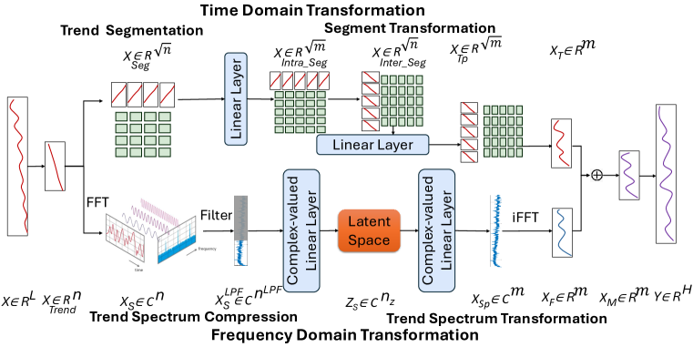
Figure 2: Architecture of MixLinear. MixLinear first extracts the trend information by downsampling the time series with a period of $w$. In the time domain, it divides the trend into segments and applies two linear transformations: one to capture intra-segment dependencies and the other to capture inter-segment dependencies. In the frequency domain, it performs the Fast Fourier Transform (FFT) to project the data into the frequency domain, followed by a low pass filter and two complex-valued linear layers for spectral compression and reconstruction. The inverse FFT (iFFT) is then used to revert the data back to the time domain. Finally, the outputs from both time and frequency domains are merged and the data is upsampled by the same period $w$.

Current research in LTSF focuses on efficiently decomposing and capturing temporal dependencies from the time or frequency domain. The key innovation of MixLinear lies in its ability to extract features from both domains while minimizing the number of neural network parameters. However, combining time and frequency domain models can significantly increase the parameter scale. MixLinear addresses such an issue by substantially reducing the parameter count without compromising prediction performance. Figure 2 illustrates the overall architecture of MixLinear, which consists of two key processes: Time Domain Transformation and Frequency Domain Transformation. Unlike the existing linear models that apply pointwise transformations, our Time Domain Transformation captures inter-segment and intra-segment dependencies by splitting the decoupled time series (trend) into segments. Such a method significantly reduces the model parameter scale and enhances the locality, which is unavailable in the pointwise methods. In contrast to the existing frequency-based models that perform transformation on the entire series, our Frequency Domain Transformation focuses on transforming more compact trend components in a lower-dimensional latent space, which reduces the model complexity by learning frequency variations more effectively. The overview workflow of MixLinear can be found in Appendix A.2.

3.2 Time Domain Transformation

The existing lightweight linear models, such as SparseTSF (Lin et al., 2024), decouple the periodic and trend components and apply a pointwise linear transformation to the trend components. In contrast, Time Domain Transformation in MixLinear divides the trend components into smaller segments and applies two linear transformations to capture intra-segment and inter-segment dependencies. Such an approach significantly reduces the model complexity while enhancing the locality of the model which is not available at the point level (Nie et al., 2023). Time Domain Transformation includes two main subprocesses: Trend Segmentation and Segment Transformation.

Trend Segmentation.

Given the time series data $X\in\mathbb{R}^{L}$ with the period $w$, we perform aggregation and downsampling to extract the trend components (Lin et al., 2024). For aggregation, we apply a 1D convolution with a kernel size of $w$, which allows us to aggregate all the information within each period at every time step. We then downsample the aggregated series by the period $w$, resulting in the trend component $X_{\text{Trend}}\in\mathbb{R}^{n}$, where $n=\left\lceil\frac{L}{w}\right\rceil$. This method effectively decouples the periodic and trend components, providing a more compact representation in which each trend time point encapsulates all the information from one period in the original series. Also, we do zero padding to $X_{\text{Trend}}$ to make $\sqrt{n}$ to be an integer. And then we split the trend components $X_{\text{Trend}}\in\mathbb{R}^{n}$ into smaller trend segments $X_{\text{Seg}}\in\mathbb{R}^{\sqrt{n}}$. We select the segment length as $\sqrt{n}$ to minimize the parameter size.

Segment Transformation.

Segment Transformation begins by applying a linear layer to trend segments $X_{\text{Seg}}$ to capture intra-segment dependencies. This produces the intra-segment prediction $X_{\text{Intra\_Seg}}\in\mathbb{R}^{\sqrt{m}}$, where $m=\lceil\frac{H}{w}\rceil$ and $H$ is the forecast horizon. $X_{\text{Intra\_Seg}}$ is then upsampled by $\sqrt{n}$, transposed, and downsampled by $\sqrt{m}$ to obtain the inter-segment series $X_{\text{Inter\_Seg}}\in\mathbb{R}^{\sqrt{n}}$. Another linear layer is applied to the inter-segment series $X_{\text{Inter\_Seg}}$ to obtain the inter-segment prediction $X_{\text{Tp}}\in\mathbb{R}^{\sqrt{m}}$. Finally, $X_{\text{Tp}}$ is upsampled by $\sqrt{m}$ to produce the time-domain output $X_{\text{T}}\in\mathbb{R}^{m}$. Leveraging Segment Transformation, MixLinear reduces the model complexity from $n\times m$ to $2\times\sqrt{n}\times\sqrt{m}$. When $m=n$, this method offers a significant reduction in complexity (from $O(n^{2})$ to $O(n)$). In addition, both inter-segment and intra-segment variations are captured.

3.3 Frequency Domain Transformation

The frequency domain representation of time series data promises a more compact and efficient portrayal of inherent patterns (Xu et al., 2024). Unlike FITS, MixLinear applies frequency domain transformation to downsampled time series subsequences (trend) and learns the frequency feature from latent space which focuses on the important bits of the data and trains in a lower dimensional, computationally much more efficient space (Rombach et al., 2022). It has two subprocesses: Trend Spectrum Compression and Trend Spectrum Transformation.

Trend Spectrum Compression.

Given the time series data $X\in\mathbb{R}^{L}$ with the period $w$, we first decompose the trend components to get $X_{Trend}\in\mathbb{R}^{n}$, where $n=\left\lceil\frac{L}{w}\right\rceil$. Then we apply FFT to the trend components $X_{Trend}$ and convert it into the frequency domain. The FFT computation for a discrete sequence $\{x_{k}\}_{k=0}^{n-1}$ is given by:

$$\bm{X}_{\text{S}}[k]=\sum_{m=0}^{n-1}x_{m}\cdot e^{-j\frac{2\pi}{n}km},$$ (1)

where $j$ is the imaginary unit, $k$ is the frequency index, and $m$ is the time index (Xu et al., 2024). $X_{S}\in\mathbb{C}^{n}$ is a complex-valued representation that concisely encapsulates the amplitude and phase of each frequency component in the Fourier domain. This transformation effectively converts the time-domain sequence into its frequency-domain representation, which captures key amplitude and phase features.

Next, we apply a Low-Pass Filter (LPF) to $X_{S}$ to remove the high-frequency components typically associated with noise and preserve the lower-frequency components that are more relevant for forecasting (Xu et al., 2024). A specified cutoff threshold is used to discard high-frequency components. LPF converts the complex-valued spectral $X_{S}\in\mathbb{C}^{n}$ to $X^{LPF}_{S}\in\mathbb{C}^{n^{LPF}}$, where $n^{LPF}$ is the cutoff frequency threshold, which is smaller than $n$.

Finally, MixLinear compresses the filtered spectral representation, $X^{LPF}_{S}$, into a lower-dimensional latent space. Specifically, a complex-valued linear layer is applied to the filtered spectral data to obtain the latent frequency space representation, $Z_{S}\in\mathbb{C}^{n_{z}}$.

Trend Spectrum Transformation.

Trend Spectrum Transformation reconstructs the trend spectrum from the latent space, and transforms it back to its original form by upsampling. The process applies a complex-valued linear layer to the latent space representation $Z_{S}\in\mathbb{C}^{n_{z}}$, transforms it into the spectrum $X_{Sp}\in\mathbb{C}^{m}$. Such a transformation is achieved through the operation $X_{Sp}=W\cdot Z_{S}+b$, where $W$ is a complex-valued weight matrix and $b$ is a bias term.

Once the spectrum $X_{Sp}$ is obtained, the iFFT is applied to convert the spectrum back to the time domain. The iFFT is mathematically defined as:

$$X_{F}(n)=\frac{1}{m}\sum_{k=0}^{m-1}X_{Sp}(k)e^{i2\pi kn/m},$$ (2)

where $m$ is the length of the spectrum, $X_{Sp}(k)$ represents the frequency domain values for each frequency $k$, and $e^{i2\pi kn/m}$ is the complex exponential term used to translate frequency components back into the time domain. This operation results in the time-domain signal $X_{F}\in\mathbb{R}^{m}$, which represents the trend prediction in the frequency domain.

The total parameter size used in the frequency domain is $(m+n)*n_{z}$. When $m=n$. the total parameter required becomes $2n*n_{z}$. As $n_{z}\ll n$, those two linear transformations reduces the parameter scale from $O(n^{2})$ to $O(n)$. We set $n_{z}$ to $2$ in the experiment section to reduce the parameter scale as much as possible.

4 Experiment

In this section, we first outline our experimental setup. We then compare MixLinear with the baseline models and assess its effectiveness in achieving high forecasting accuracy with minimal parameters by integrating both time and frequency domain features. Lastly, we evaluate the generalization capability of MixLinear. Detailed analyses of MixLinear’s performance in ultra-long period scenarios, as well as the impact of the low-pass filter cutoff frequency, are provided in the appendix.

4.1 Experiment Setup

Datasets.

We perform experiments with four benchmark LTSF datasets (i.e., ETTh1, ETTh2, Electricity, and Traffic) that exhibit daily periodicity. The ETTh1 and ETTh2 datasets contain hourly data collected from Informer (Zhou et al., 2021). The Electricity dataset contains the hourly electricity consumption of $321$ customers from the University of California, Irvine Machine Learning Repository website. The Traffic dataset is a collection of hourly data from the California Department of Transportation. More details about those datasets can be found in Appendix A.1.

Baselines.

We conduct a comparative analysis of MixLinear against state-of-the-art baselines in the field, including FEDformer (Zhou et al., 2022b), TimesNet (Wu et al., 2022), and PatchTST (Nie et al., 2023). In addition, we compare MixLinear against three lightweight models: DLinear (Zeng et al., 2023), FITS (Xu et al., 2024), and SparseTSF (Lin et al., 2024). More details about those baselines can be found in Appendix A.3.

Environment.

MixLinear and our baselines are implemented using PyTorch (Paszke et al., 2019). All experiments are performed on a single NVIDIA A100 GPU with $80GB$ of memory. More details on our experimental setup are presented in Appendix A.4.

4.2 Prediction Performance

Table 1: MSE results of multivariate long-term time series forecasting comparing MixLinear against baselines. The top three results are highlighted in bold. The best results are in bold and underlined. “Imp.” denotes the improvement compared to the best-performing baseline.

Dataset		ETTh1				ETTh2				Electricity				Traffic
Horizon		96	192	336	720	96	192	336	720	96	192	336	720	96	192	336	720
FEDformer (2022)		0.375	0.427	0.459	0.484	0.340	0.433	0.508	0.480	0.188	0.197	0.212	0.244	0.573	0.611	0.621	0.630
TimesNet (2023)		0.384	0.436	0.491	0.521	0.340	0.402	0.452	0.462	0.168	0.184	0.198	0.220	0.593	0.617	0.629	0.640
PatchTST (2023)		0.385	0.413	0.440	0.456	0.274	0.338	0.367	0.391	0.129	0.149	0.166	0.210	0.366	0.388	0.398	0.457
DLinear (2023)		0.384	0.443	0.446	0.504	0.282	0.340	0.414	0.588	0.140	0.153	0.169	0.204	0.413	0.423	0.437	0.466
FITS (2024)		0.382	0.417	0.436	0.433	0.272	0.333	0.355	0.378	0.145	0.159	0.175	0.212	0.398	0.409	0.421	0.457
SparseTSF (2024)		0.362	0.403	0.434	0.426	0.294	0.339	0.359	0.383	0.138	0.151	0.166	0.205	0.389	0.398	0.411	0.448
MixLinear (ours)		0.351	0.395	0.411	0.423	0.283	0.337	0.356	0.380	0.138	0.154	0.170	0.209	0.389	0.403	0.416	0.452
Imp.		+0.011	+0.008	+0.023	+0.003	-0.011	-0.004	-0.001	-0.002	-0.009	-0.002	-0.004	-0.005	-0.023	-0.015	-0.018	-0.004

We first evaluate MixLinear with four benchmark LTSF datasets. Table 1 lists the MSE values of prediction accuracy under MixLinear and our baseline models at the forecast horizons of $96$, $192$, $336$, and $720$.

Performance in Low-Channel Scenarios.

As Table 1 shows, MixLinear demonstrates strong performance in scenarios with fewer channels ($7$ channels), such as the ETTh1 and ETTh2 datasets. For instance, on ETTh1, MixLinear outperforms the baseline models, achieving the lowest MSE values of $0.351$, $0.395$, $0.411$, and $0.423$ at forecast horizons of $96$, $192$, $336$, and $720$, respectively. Specifically, MixLinear achieves an MSE reduction of $5.3\%$ ($+0.023$) on ETTh1 at the forecast horizon of $336$. On ETTh2, MixLinear ranks within the top two models across all horizons, except at the horizon of $96$. These results highlight that our linear time-domain and frequency-domain decomposition method is well-suited for datasets with fewer channels.

Performance in High-Channel Scenarios.

Table 1 further shows that MixLinear consistently delivers strong performance on datasets with a higher number of channels, such as Electricity ($321$ channels) and Traffic ($862$ channels). MixLinear ranks within the top two across most cases when compared with lightweight models like DLinear, FITS, and SparseTSF. Even when compared with parameter-heavy models, MixLinear still ranks within the top three in the majority of cases. Notably, MixLinear achieves this performance with only $0.1K$ parameters, significantly fewer than the baseline models, which require $6M$ parameters for PatchTST, $10K$ parameters for FITS, and $1K$ parameters for SparseTSF.

Performance at Extended Horizons.

At the extended forecast horizon of $720$, MixLinear consistently ranks within the top two models across all datasets, with the exception of the Electricity dataset (see Table 1). On ETTh1, MixLinear reduces the MSE by $0.003$ at the $720$ forecast horizon. On other datasets, the MSE increase at this horizon remains under $0.005$. These findings highlight the robustness of MixLinear in handling long-term forecasting tasks effectively.

The experimental results with the dataset with ultra-long periods can be found in Appendix B.1.

4.3 Efficiency

Table 2: Static and runtime metrics of MixLinear and the baselines on the Electricity dataset with a forecast horizon $720$. The look-back length for each model is set to the default value used in those papers.

Model	Parameters	MACs	Time(s)	MSE
Informer (2021)	12.53M	3.97G	70.1	0.373
Autoformer (2021)	12.92M	4.41G	107.7	0.254
FEDformer (2022)	17.98M	4.41G	238.7	0.244
FiLM (2022)	12.22M	4.41G	78.3	0.236
PatchTST (2023)	6.31M	11.21G	290.4	0.210
DLinear (2023)	485.3K	156M	36.2	0.204
FITS (2024)	10.5K	79.9M	25.7	0.212
SparseTSF (2024)	0.92K	12.71M	33	0.205
MixLinear (Ours)	0.195K	9.86M	23.9	0.209

To examine the efficiency of MixLinear, we measure three static and runtime metrics including:

• Parameters: The number of parameters in the model. This is a measure of the model’s complexity.

• MACs: The number of multiply-accumulate operations required per prediction. This is a measure of the model’s computational cost.

• Time(s): The amount of time (in seconds) it takes to train the model for one epoch. An epoch is one pass through the entire training dataset.

Table 2 lists the measurements when we apply MixLinear and our baselines on the Electricity dataset with a forecast horizon of $720$. As Table 2 lists, MixLinear is the most computationally efficient model among all solutions. To achieve a good prediction accuracy ($MSE=0.209$), it only needs $0.195K$ parameters and $9.86M$ MACs, and provides the shortest training time of $23.9s$ per epoch. As a comparison, DLinear requires $485.3K$ parameters, $156M$ MACs, and a training time of $36.2s$ per epoch to achieve the best prediction accuracy ($MSE=0.204$). The slight decreases in prediction accuracy are in exchange for a proportionally much larger enhancement in efficiency. We observe similar results in other datasets. The results show that MixLinear is well-suited for the scenarios where the computational resources are limited.

4.4 Effectiveness of Mixing the Time and Frequency Domain

Table 3: MSE results of multivariate LTSF with MixLinear when disabling part of the modules.

Dataset		ETTh1				ETTh2				Electricity				Traffic
Horizon		96	192	336	720	96	192	336	720	96	192	336	720	96	192	336	720
TLinear		0.376	0.398	0.412	0.425	0.317	0.366	0.369	0.389	0.181	0.192	0.209	0.245	0.485	0.483	0.520	0.528
FLinear		0.434	0.438	0.473	0.474	0.364	0.381	0.383	0.411	0.171	0.179	0.191	0.248	0.397	0.436	0.442	0.478
MixLinear		0.351	0.395	0.411	0.423	0.283	0.337	0.356	0.380	0.138	0.154	0.170	0.209	0.384	0.398	0.416	0.451

To evaluate the effectiveness of mixing time and frequency domain features, we compare MixLinear against two altered versions: TLinear and FLinear. TLinear is created by disabling the transformation in the frequency domain in MixLinear, while FLinear is implemented by disabling the transformation in the time domain. As Table 3 lists, TLinear achieves better performance on the ETTh1 and ETTh2 datasets compared to FLinear in the low-channel scenario. In the high-channel scenario, including the Electricity dataset with $321$ channels and the Traffic dataset with $862$ channels, FLinear tends to perform better. The reason behind is that the trend components of the time series data in the time domain are relatively easy to capture when there are a small number of channels because the model can focus on the long-term patterns in the individual time series. On the other hand, capturing the trend components becomes more effective in the frequency domain when facing a large number of variates, because the decomposition into different frequency bands benefits from the diversity of the channels. MixLinear outperforms both TLinear and FLinear in all cases because both Time Domain Transformation and Frequency Domain Transformation contribute significantly to the model’s high forecasting accuracy.

4.5 Generalization Ability of the MixLinear Model

Table 4: Comparison of generalization capabilities between MixLinear and other mainstream models. “Dataset A $\rightarrow$ Dataset B” denotes the training and validation on the training and validation sets of Dataset A, followed by testing on the test set of Dataset B.

Dataset	ETTh2 $\rightarrow$ ETTh1				Electricity $\rightarrow$ ETTh1
Horizon	96	192	336	720	96	192	336	720
Informer (2021)	0.844	0.921	0.898	0.829	\	\	\	\
Autoformer (2021)	0.978	1.058	0.944	0.921	\	\	\	\
FEDformer (2022)	0.878	0.927	0.929	0.976	\	\	\	\
FiLM (2022)	0.876	0.904	0.919	0.925	\	\	\	\
PatchTST (2023)	0.449	0.478	0.426	0.400	0.424	0.475	0.472	0.470
DLinear (2023)	0.430	0.478	0.458	0.506	0.397	0.424	0.477	0.470
FiTs (2024)	0.419	0.427	0.428	0.445	0.380	0.414	0.440	0.448
SparseTSF (2024)	0.370	0.401	0.412	0.419	0.373	0.409	0.433	0.439
MixLinear (Ours)	0.361	0.388	0.406	0.427	0.373	0.410	0.428	0.434

MixLinear enhances forecasting ability by combining time and frequency domain features, improving generalization across datasets with similar periodicities. To explore this, we examined the cross-domain generalization performance of the MixLinear model by training on one dataset and testing on another. We compare MixLinear with several other mainstream models for multivariate LTSF in two scenarios: training and validation on ETTh2 with testing on ETTh1, and training and validation on Electricity with testing on ETTh1. As Table 4 lists, MixLinear has the best generalization ability and consistently achieves the lowest MSE values on different datasets and prediction horizons. When we train the model on ETTh2 and validate it on ETTh1, MixLinear achieves the lowest MSE at forecast horizons of $96$, $192$, and $336$. Similarly, when we train the model on Electricity and validate it on ETTh1, it achieves the lowest MSE at horizons of $96$, $336$, and $720$, and offers an MSE of $0.410$ at the $192$ horizon which is just $0.001$ higher than the best-performing model, SparseTSF ($0.409$). By combining features from both time and frequency domains, MixLinear can avoid the shortcut learning (Geirhos et al., 2020) problem, which occurs when the model focuses on time-space features while overlooking crucial underlying concepts in the frequency-space domain or vice versa, leading to limited poor performance on data unseen during training (He et al., 2023). The results highlight the effectiveness of MixLinear in transferring knowledge learned from one dataset to another by combining both time domain and frequency domain features, which demonstrates its robustness and adaptability in various forecasting scenarios.

5 Related Work

5.1 Long-term Time Series Forecasting

LTSF aims to predict future values over extended horizons, which is challenging because the time series data is complex and high-dimensional Zheng et al. (2024; 2023). The traditional statistical methods, such as ARIMA (Contreras et al., 2003) and Holt-Winters (Chatfield & Yar, 1988), are effective for short-term forecasting but often fall short for long-term predictions. Machine learning models, such as SVM (Wang & Hu, 2005), Random Forests Breiman (2001), and Gradient Boosting Machines (Natekin & Knoll, 2013), have improved performance by capturing non-linear relationships but require extensive feature engineering. Recently, deep learning models, such as RNNs, LSTMs, GRUs, and Transformer-based models including Informer and Autoformer have excelled in efficiently modeling long-term dependencies. The hybrid models that combine statistical and machine learning or deep learning techniques have also shown enhanced accuracy. State-of-the-art models like FEDformer (Zhou et al., 2022b), FiLM (Zhou et al., 2022a), PatchTST Nie et al. (2023), and SparseTSF incorporate advanced mechanisms like frequency domain transformations and efficient self-attention to achieve remarkable performance.

Recently, there has been a notable trend towards designing lightweight LTSF models. DLinear (Zeng et al., 2023) shows that even simple models can capture significant temporal periodic dependencies effectively. LightTS (Campos et al., 2023), TiDE (Das et al., 2023), and TSMixer (Chen et al., 2023) show similar conclusions. FITS (Xu et al., 2024) has emerged as a significant advancement in the field and achieved a milestone by scaling LTSF models to around $10K$ parameters while maintaining high predictive accuracy. FITS accomplishes this by transforming time-domain forecasting tasks into frequency-domain equivalents and employing low-pass filters to minimize parameter requirements. SparseTSF (Lin et al., 2024) pushes the boundaries even further by leveraging the Cross-Period Sparse Forecasting technique.

5.2 Time Series Data Decomposition

Several decomposition methods in the time domain have been introduced in the literature to handle such a task, including STL (Robert, 1990), TBATS (De Livera et al., 2011), and STR (Dokumentov et al., 2015) for periodic series, as well as $l_{1}$ trend filtering (Moghtaderi et al., 2011) and mixed trend filtering (Tibshirani, 2014) for non-periodic data. Although these techniques have gained popularity and proven effective in various applications, they exhibit limitations due to three reasons: the inefficiency in handling time series with long seasonal periods, the frequent seasonal shifts and fluctuations in real-world data, and the lack of robustness to outliers and noise (Gao et al., 2020).

Decomposing time series data in the frequency domain provides compressed representations that capture rich underlying patterns (Xu et al., 2020). These representations offer a more compact and efficient depiction of the inherent characteristics within the data (Xu et al., 2024). FEDformer decomposes sequences into multiple frequency domain modes using frequency transforms to extract features (Zhou et al., 2022b). TimesNet (Wu et al., 2022) employs a frequency-based method to separate intraperiod and interperiod variations. FITS (Xu et al., 2024) leverages this property by transforming the time series into the frequency domain, treating the data as a signal that can be expressed as a linear combination of sinusoidal components, a process that ensures no information loss. Each sinusoidal component is defined by its own frequency, amplitude, and initial phase, allowing for a precise representation of different oscillatory patterns present in the data. Although there are many ways of frequency domain decomposition method, extracting features from the frequency domain requires suitable techniques. There will be many interferences in the signal, and suitable schemes for temporal features must be considered when combining deep learning methods.

6 Conclusion

There has been a growing interest in LTSF, which aims to predict long-term future values by identifying patterns and trends in large amounts of historical time-series data. A key challenge in LTSF is to manage long sequence inputs and outputs without incurring excessive computational or memory overhead, particularly in resource-constrained scenarios. In this paper, we introduce MixLinear, the first lightweight LTSF model that captures temporal and frequency features from both time and frequency domains. MixLinear applies the trend segmentation in the time domain to capture the intra-segment and inter-segment variations and captures the amplitude and phase information by reconstructing the trend spectrum from a low dimensional frequency domain latent space. Experimental results show that MixLinear can achieve comparable or better forecasting accuracy with only $0.1K$ parameters. Besides, MixLinear exhibits strong generalization capability and is well-suited for scenarios where the training data are limited.

Appendix A More Details of MixLinear

A.1 Detailed Dataset Description

Table 5: Statistics of seven datasets.

Dataset	Traffic	Electricity	Weather	ETTh1	ETTh2	ETTm1	ETTm2
Channels	862	321	21	7	7	7	7
Sampling Rate	1 hour	1 hour	10 min	1 hour	1 hour	15 min	15 min
Total Timesteps	17,544	26,304	52,696	17,420	17,420	69,680	69,680

The seven benchmark datasets used in our experiments are as follows:

(1) The ETT dataset, sourced from Informer (Zhou et al., 2021), consists of data collected every 15 minutes between July 2016 and July 2018, including load and oil temperature readings. The ETTh1 and ETTh2 subsets are sampled at 1-hour intervals, while ETTm1 and ETTm2 are sampled at 15-minute intervals.

(2) The Electricity dataset contains the hourly electricity consumption of 321 customers, spanning the period from 2012 to 2014.

(3) The Traffic dataset comprises hourly road occupancy rates, recorded by sensors placed on freeways in the San Francisco Bay Area. The data is provided by the California Department of Transportation.

(4) The Weather dataset includes local climatological data collected from approximately 1,600 locations across the United States, spanning a period of four years (2010 to 2013). Data points are recorded at 1-hour intervals.

A.2 Overview Workflow

1

Input : Historical look-back window $x_{t-L+1:t}\in\mathbb{R}^{L}$ and its period $w$

Output : Forecasted output $\hat{x}_{t+1:t+H}\in\mathbb{R}^{H}$

2

3

41:$x_{mean}\leftarrow\frac{1}{L}\sum_{i=t-L+1}^{t}x_{i}$ $\triangleright$ Compute the mean value of the historical look-back window

52:$x_{norm}\leftarrow x_{t-L+1:t}-x_{mean}$ $\triangleright$ Normalize the input by subtracting the mean

63:$x_{norm}\leftarrow\text{Conv1d}(x_{norm},w)+x_{norm}$ $\triangleright$ Apply a 1D convolution over the normalized input sequence

74:$n\leftarrow\lceil L/w\rceil$ $\triangleright$ Determine the downsampled sequence length $n$

85:$x_{trend}\leftarrow\text{Reshape}(x,(n,w))$ $\triangleright$ Reshape the input into an $n\times w$ matrix for further processing

96:$\hat{n}\leftarrow\lceil\sqrt{\text{n}}\rceil^{2}$ $\triangleright$ Adjust the sequence length $\hat{n}$ to ensure $\sqrt{\hat{n}}$ is an integer

107:$x_{trend}\leftarrow\text{Pad}(x_{trend},(\hat{n}-n))$ $\triangleright$ Apply zero-padding to extend the length $n$ to $\hat{n}$

118:$X_{Seg}\leftarrow\text{Reshape}(x_{trend},(\sqrt{\hat{n}},\sqrt{\hat{n}}))$ $\triangleright$ Reshape the trend data into a $\sqrt{\hat{n}}\times\sqrt{\hat{n}}$ matrix

129:$X_{Tp}\leftarrow\text{Linear}(\text{Linear}(X_{Seg})^{T})^{T}$ $\triangleright$ Apply two linear transformations

1310:$m\leftarrow\lceil H/w\rceil$ $\triangleright$ Compute the downsampled length of the forecast horizon $m$

1411:$x_{T}\leftarrow\text{Reshape}(X_{Tp},m)$ $\triangleright$ Reshape $X_{Tp}$ into a sequence of length $m$ for the forecast

1512:$x_{\text{S}}\leftarrow\text{FFT}(x_{trend})$ $\triangleright$ Apply the FFT on the trend data with Equation 1

1613:$x^{LPF}_{\text{S}}\leftarrow\text{LPF}(x_{\text{S}},n^{LPF})$ $\triangleright$ Apply a low-pass filter to the frequency-domain representation to reduce noise

1714:$z_{\text{S}}\leftarrow\text{Linear}(x^{LPF}_{\text{S}})$ $\triangleright$ Project the filtered frequency components into a latent space using a linear transformation

1815:$x_{\text{Sp}}\leftarrow\text{Linear}(z_{\text{S}})$ $\triangleright$ Apply a linear transformation to the latent frequency representation

1916:$x_{\text{F}}\leftarrow\text{iFFT}(x_{\text{Sp}})$ $\triangleright$ Apply the iFFT to reconstruct the frequency domain signal with Equation 2

2017:$x_{M}\leftarrow x_{T}+x_{F}+c_{mean}$ $\triangleright$ Combine the time-domain and frequency-domain components and add back the mean

2118:$\hat{x}_{t+1:t+H}\leftarrow\text{Reshape}(x_{M},H)$ $\triangleright$ Reshape the combined signal back into a sequence of length $H$ for the forecast output

Algorithm 1 Overall Pseudocode of MixLinear

The complete workflow of MixLinear is outlined in Algorithm 1, which takes a univariate historical look-back window $x_{t-L+1:t}$ as input and outputs the corresponding forecast results $\hat{x}_{t+1:t+H}$. Multivariate time series forecasting can be effectively achieved by integrating the CI strategy, i.e., modeling multiple channels using a model with shared parameters.

A.3 Detailed Baseline Model Description

We briefly describe the baseline models we used in this paper:

(1) Informer is a Transformer-based model that employs self-attention distillation to highlight dominant attention by halving the input to cascading layers, enabling efficient handling of extremely long input sequences. The source code is available at https://github.com/zhouhaoyi/Informer2020.

(2) Autoformer is a Transformer-based model that introduces the Auto-Correlation mechanism, leveraging the periodicity of time series to discover dependencies and aggregate representations at the sub-series level. The source code is available at https://github.com/thuml/Autoformer.

(3) Pyraformer is a Transformer-based model that captures temporal dependencies of different ranges in a compact multi-resolution fashion. The source code is available at https://github.com/ant-research/Pyraformer.

(4) FEDformer (Zhou et al., 2022b) is a Transformer-based model proposing seasonal-trend decomposition and exploiting the sparsity of time series in the frequency domain. The source code is available at https://github.com/DAMO-DI-ML/ICML2022-FEDformer.

(5) TimesNet (Wu et al., 2022) is a CNN-based model with TimesBlock as a task-general backbone. It transforms 1D time series into 2D tensors to capture intraperiod and interperiod variations. The source code is available at https://github.com/thuml/TimesNet.

(6) PatchTST (Nie et al., 2023) is a transformer-based model utilizing patching and CI technique. It also enables effective pre-training and transfer learning across datasets. The source code is available at https://github.com/yuqinie98/PatchTST.

(7) DLinear (Zeng et al., 2023) is an MLP-based model with just one linear layer, which outperforms Transformer-based models in LTSF tasks. The source code is available at https://github.com/cure-lab/LTSF-Linear.

(8) FITS (Xu et al., 2024) is a linear model that manipulates time series data through interpolation in the complex frequency domain. The source code is available at https://github.com/VEWOXIC/FITS.

(9) SparseTSF (Lin et al., 2024) is a novel, extremely lightweight model for LTSF, designed to address the challenges of modeling complex temporal dependencies over extended horizons with minimal computational resources. The source code is available at https://github.com/lss-1138/SparseTSF.

A.4 Detailed Experimental Setup

We implement MixLinear in PyTorch (Paszke et al., 2019) and train it using the Adam optimizer (Diederik, 2015) for $30$ epochs with early stopping based on a patience of 10 epochs. We follow the procedures outlined in FITS and Autoformer to split the dataset (Wu et al., 2021). Specifically, the ETT datasets are divided into training, validation, and test sets with a $6:2:2$ ratio. The other datasets are split with a $7:1:2$ ratio.

MixLinear has minimal hyperparameters due to its simple design. The period $w$ is chosen based on the inherent cycle of the data (e.g., $w=24$ for the ETTh1 dataset) or reduced when the dataset exhibits a longer cycle. The batch size is determined by the number of channels in each dataset. The batch size is set to $256$ for the datasets with fewer than $100$ channels (e.g., ETTh1). The batch size is set to $128$ for the datasets with fewer than $300$ channels (e.g., Electricity). Such a configuration maximizes the GPU parallelism while preventing any out-of-memory issues. In addition, given the small number of learnable parameters in MixLinear, we use a relatively large learning rate of $0.02$ to accelerate training.

The baseline results reported in this paper come from the first version of the FITS paper, where FITS uses a uniform input length of $720$. To ensure a fair comparison, we also use an input length of $720$. The input lengths of other baseline models are set according to the values used in their original implementations.

Appendix B More results and analysis

In this section, we evaluate MixLinear with the ultra-long period datasets and examine the effect of the low-pass filter cutoff frequency thresholds on its performance.

B.1 Ultra-long Period Scenario

Table 6: MSE results on the datasets with ultra-long periods.

Dataset	ETTm1				ETTm2				Weather
Horizon	96	192	336	720	96	192	336	720	96	192	336	720
Informer (2021)	0.672	0.795	1.212	1.166	0.365	0.533	1.363	3.379	0.300	0.598	0.578	1.059
Autoformer (2021)	0.505	0.553	0.621	0.671	0.255	0.281	0.339	0.433	0.266	0.307	0.359	0.419
Pyraformer (2022b)	0.543	0.557	0.754	0.908	0.435	0.730	2.308	3.625	0.389	0.622	0.739	1.004
FEDformer (2022b)	0.379	0.426	0.445	0.543	0.203	0.269	0.325	0.421	0.217	0.276	0.339	0.403
TimesNet (2023)	0.338	0.374	0.410	0.478	0.187	0.249	0.321	0.408	0.172	0.219	0.280	0.365
PatchTST (2023)	0.293	0.333	0.369	0.416	0.166	0.223	0.274	0.362	0.149	0.194	0.245	0.314
DLinear (2023)	0.299	0.335	0.369	0.425	0.167	0.221	0.274	0.368	0.176	0.218	0.262	0.323
FITS (2024)	0.305	0.339	0.367	0.418	0.164	0.217	0.269	0.347	0.145	0.188	0.236	0.308
SparseTSF (2024)	0.314	0.343	0.369	0.418	0.165	0.218	0.272	0.350	0.172	0.215	0.260	0.318
MixLinear (ours)	0.332	0.353	0.385	0.437	0.170	0.223	0.275	0.360	0.172	0.212	0.257	0.324

To evaluate the prediction performance of MixLinear in ultra-long period forecasting scenarios, we conduct additional experiments using the ETTm1, ETTm2, and Weather datasets. Table 6 presents the MSE values achieved by MixLinear and the baseline models when applied to ultra-long period forecasting tasks. As Table 6 shows, MixLinear demonstrates competitive performance across these datasets, with only $0.1K$ parameters, and even surpasses several transformer-based models that employ millions of parameters, including Informer, Autoformer, PyraFormer, and FEDFormer.

B.2 Effect of low pass filter cutoff frequency on performance

Table 7: MSE results of multivariate LTSF using MixLinear with different LPF.

Dataset		ETTh1				ETTh2				Electricity				Traffic
Horizon		96	192	336	720	96	192	336	720	96	192	336	720	96	192	336	720
MixLinear ($n^{LPF}$=1)		0.351	0.399	0.412	0.440	0.289	0.353	0.373	0.386	0.170	0.184	0.202	0.238	0.449	0.450	0.469	0.510
MixLinear ($n^{LPF}$=5)		0.356	0.395	0.412	0.426	0.290	0.349	0.360	0.389	0.151	0.163	0.179	0.243	0.407	0.422	0.430	0.473
MixLinear ($n^{LPF}$=10)		0.376	0.397	0.413	0.425	0.294	0.341	0.357	0.387	0.171	0.155	0.171	0.210	0.396	0.411	0.417	0.454
MixLinear ($n^{LPF}$=15)		0.358	0.398	0.413	0.427	0.284	0.343	0.356	0.383	0.139	0.154	0.171	0.209	0.392	0.404	0.421	0.454
MixLinear ($n^{LPF}$=19)		0.360	0.396	0.413	0.423	0.283	0.337	0.359	0.380	0.139	0.154	0.171	0.209	0.390	0.406	0.416	0.452

To evaluate the effect of the cutoff frequency used by the low-pass filter, we vary the LPF cutoff frequency threshold from $1$ to $19$ across the forecast horizons of $96$, $192$, $336$, and $720$ and measure MixLinear’s prediction performance. As Table 7 lists, the prediction performance of MixLinear decreases significantly as the LPF threshold decreases from $5$ to $1$. To achieve a balance between performance and computational efficiency, a cutoff frequency of $5$ is generally optimal for resource-constrained environments. However, the performance on the ETTh2 dataset is less sensitive to variations in the LPF cutoff frequency. The results indicate that while the LPF can help reduce the model complexity, a more adaptive filtering strategy may be required for LTSF tasks to maintain optimal performance.

References

- Breiman (2001) Leo Breiman. Random forests. Machine Learning, 45:5–32, 2001.
- Campos et al. (2023) David Campos, Miao Zhang, Bin Yang, Tung Kieu, Chenjuan Guo, and Christian S Jensen. Lightts: Lightweight time series classification with adaptive ensemble distillation. Proceedings of the ACM on Management of Data, 1(2):1–27, 2023.
- Chatfield & Yar (1988) Chris Chatfield and Mohammad Yar. Holt-winters forecasting: some practical issues. Journal of the Royal Statistical Society Series D: The Statistician, 37(2):129–140, 1988.
- Chen et al. (2023) Si An Chen, Chun Liang Li, Nate Yoder, Sercan O Arik, and Tomas Pfister. Tsmixer: An all-mlp architecture for time series forecasting. Transactions on Machine Learning Research, 2023.
- Cirstea et al. (2022) Razvan-Gabriel Cirstea, Chenjuan Guo, Bin Yang, Tung Kieu, Xuanyi Dong, and Shirui Pan. Triformer: Triangular, variable-specific attentions for long sequence multivariate time series forecasting–full version. In International Joint Conference on Artificial Intelligence (IJCAI), 2022.
- Contreras et al. (2003) Javier Contreras, Rosario Espinola, Francisco J Nogales, and Antonio J Conejo. Arima models to predict next-day electricity prices. IEEE Transactions on Power Systems, 18(3):1014–1020, 2003.
- Das et al. (2023) Abhimanyu Das, Weihao Kong, Andrew Leach, Shaan Mathur, Rajat Sen, and Rose Yu. Long-term forecasting with tide: Time-series dense encoder. Transactions on Machine Learning Research, 2023.
- De Livera et al. (2011) Alysha M De Livera, Rob J Hyndman, and Ralph D Snyder. Forecasting time series with complex seasonal patterns using exponential smoothing. Journal of the American Statistical Association, 106(496):1513–1527, 2011.
- Diederik (2015) P Kingma Diederik. Adam: A method for stochastic optimization. International Conference on Learning Representations (ICLR), 2015.
- Dokumentov et al. (2015) Alexander Dokumentov, Rob J Hyndman, et al. Str: A seasonal-trend decomposition procedure based on regression. INFORMS Journal on Data Science, 13(15):2015–13, 2015.
- Gao et al. (2020) Jingkun Gao, Xiaomin Song, Qingsong Wen, Pichao Wang, Liang Sun, and Huan Xu. Robusttad: Robust time series anomaly detection via decomposition and convolutional neural networks. In ACM SIGKDD Workshop on Mining and Learning from Time Series (KDD-MiLeTS), 2020.
- Gardner Jr (1985) Everette S Gardner Jr. Exponential smoothing: The state of the art. Journal of Forecasting, 4(1):1–28, 1985.
- Geirhos et al. (2020) Robert Geirhos, Jörn-Henrik Jacobsen, Claudio Michaelis, Richard Zemel, Wieland Brendel, Matthias Bethge, and Felix A Wichmann. Shortcut learning in deep neural networks. Nature Machine Intelligence, 2(11):665–673, 2020.
- Harvey (1990) Andrew C Harvey. Forecasting, structural time series models and the Kalman filter. Cambridge university press, 1990.
- He et al. (2023) Huan He, Owen Queen, Teddy Koker, Consuelo Cuevas, Theodoros Tsiligkaridis, and Marinka Zitnik. Domain adaptation for time series under feature and label shifts. In International Conference on Machine Learning (ICML), 2023.
- He & Zhao (2019) Yangdong He and Jiabao Zhao. Temporal convolutional networks for anomaly detection in time series. Journal of Physics: Conference Series, 1213(4):042050, 2019.
- Kim et al. (2014) Kibaek Kim, Changhyeok Lee, Kevin O’Leary, Shannon Rosenauer, and Sanjay Mehrotra. Predicting patient volumes in hospital medicine: A comparative study of different time series forecasting methods. Scientific Report, 2014.
- Lin et al. (2024) Shengsheng Lin, Weiwei Lin, Wentai Wu, Haojun Chen, and Junjie Yang. Sparsetsf: Modeling long-term time series forecasting with 1k parameters. In International Conference on Machine Learning (ICML), 2024.
- Liu et al. (2021) Shizhan Liu, Hang Yu, Cong Liao, Jianguo Li, Weiyao Lin, Alex X Liu, and Schahram Dustdar. Pyraformer: Low-complexity pyramidal attention for long-range time series modeling and forecasting. In International Conference on Learning Representations (ICLR), 2021.
- Moghtaderi et al. (2011) Azadeh Moghtaderi, Pierre Borgnat, and Patrick Flandrin. Trend filtering: empirical mode decompositions versus l1 and hodrick–prescott. Advances in Adaptive Data Analysis, 3(01n02):41–61, 2011.
- Mohan et al. (2011) Ananth Mohan, Zheng Chen, and Kilian Weinberger. Web-search ranking with initialized gradient boosted regression trees. In Proceedings of Machine Learning Research(PMLR), 2011.
- Moon & Wettlaufer (2017) Woosok Moon and John S Wettlaufer. A unified nonlinear stochastic time series analysis for climate science. Scientific Reports, 7(1):44228, 2017.
- Nassar et al. (2004) Sameh Nassar, Klaus-Peter Schwarz, Naser Elsheimy, and Aboelmagd Noureldin. Modeling inertial sensor errors using autoregressive (ar) models. Navigation, 51(4):259–268, 2004.
- Natekin & Knoll (2013) Alexey Natekin and Alois Knoll. Gradient boosting machines, a tutorial. Frontiers in Neurorobotics, 7:21, 2013.
- Nie et al. (2022) Xingqing Nie, Xiaogen Zhou, Zhiqiang Li, Luoyan Wang, Xingtao Lin, and Tong Tong. Logtrans: Providing efficient local-global fusion with transformer and cnn parallel network for biomedical image segmentation. In High Performance Computing and Communications (HPCC), 2022.
- Nie et al. (2023) Yuqi Nie, Nam H Nguyen, Phanwadee Sinthong, and Jayant Kalagnanam. A time series is worth 64 words: Long-term forecasting with transformers. International Conference on Learning Representations (ICLR), 2023.
- Nunnari & Nunnari (2017) Giuseppe Nunnari and Valeria Nunnari. Forecasting monthly sales retail time series: a case study. In 2017 IEEE 19th Conference on Business Informatics (CBI), volume 1, pp. 1–6. IEEE, 2017.
- Paszke et al. (2019) Adam Paszke, Sam Gross, Francisco Massa, Adam Lerer, James Bradbury, Gregory Chanan, Trevor Killeen, Zeming Lin, Natalia Gimelshein, Luca Antiga, et al. Pytorch: An imperative style, high-performance deep learning library. Advances in Neural Information Processing Systems (NeurIPS), 32, 2019.
- Robert (1990) Ceveland Robert, B. Stl: A seasonal-trend decomposition procedure based on loess. Journal of Official Statistics, 6:3–73, 1990.
- Rombach et al. (2022) Robin Rombach, Andreas Blattmann, Dominik Lorenz, Patrick Esser, and Björn Ommer. High-resolution image synthesis with latent diffusion models. In IEEE/CVF Computer Vision and Pattern Recognition Conference (CVPR), 2022.
- Salehinejad et al. (2017) Hojjat Salehinejad, Sharan Sankar, Joseph Barfett, Errol Colak, and Shahrokh Valaee. Recent advances in recurrent neural networks. arXiv preprint arXiv:1801.01078, 2017.
- Sezer et al. (2020) Omer Berat Sezer, Mehmet Ugur Gudelek, and Ahmet Murat Ozbayoglu. Financial time series forecasting with deep learning: A systematic literature review: 2005–2019. Applied Soft Computing, 90:106181, 2020.
- Tibshirani (2014) Ryan J Tibshirani. Adaptive piecewise polynomial estimation via trend filtering. The Annals of Statistics, 42(1):285–3, 2014.
- Wang & Hu (2005) Haifeng Wang and Dejin Hu. Comparison of svm and ls-svm for regression. In International Conference on Neural Networks and Brain (ICNNB), 2005.
- Watson et al. (2021) Gregory L Watson, Di Xiong, Lu Zhang, Joseph A Zoller, John Shamshoian, Phillip Sundin, Teresa Bufford, Anne W Rimoin, Marc A Suchard, and Christina M Ramirez. Pandemic velocity: Forecasting covid-19 in the us with a machine learning & bayesian time series compartmental model. PLoS Computational Biology, 17(3):e1008837, 2021.
- Wu et al. (2021) Haixu Wu, Jiehui Xu, Jianmin Wang, and Mingsheng Long. Autoformer: Decomposition transformers with auto-correlation for long-term series forecasting. Advances in Neural Information Processing Systems (NeurIPS), 2021.
- Wu et al. (2022) Haixu Wu, Tengge Hu, Yong Liu, Hang Zhou, Jianmin Wang, and Mingsheng Long. Timesnet: Temporal 2d-variation modeling for general time series analysis. International Conference on Learning Representations (ICLR), 2022.
- Xu et al. (2020) Kai Xu, Minghai Qin, Fei Sun, Yuhao Wang, Yen-Kuang Chen, and Fengbo Ren. Learning in the frequency domain. In IEEE/CVF Computer Vision and Pattern Recognition Conference (CVPR), 2020.
- Xu et al. (2024) Zhijian Xu, Ailing Zeng, and Qiang Xu. Fits: Modeling time series with parameters. In International Conference on Learning Representations (ICLR), 2024.
- Zeng et al. (2023) Ailing Zeng, Muxi Chen, Lei Zhang, and Qiang Xu. Are transformers effective for time series forecasting? In Association for the Advancement of Artificial Intelligence (AAAI), 2023.
- Zheng et al. (2023) Xu Zheng, Tianchun Wang, Wei Cheng, Aitian Ma, Haifeng Chen, Mo Sha, and Dongsheng Luo. Auto tcl: Automated time series contrastive learning with adaptive augmentations. In International Joint Conference on Artificial Intelligence (IJCAI), 2023.
- Zheng et al. (2024) Xu Zheng, Tianchun Wang, Wei Cheng, Aitian Ma, Haifeng Chen, Mo Sha, and Dongsheng Luo. Parametric augmentation for time series contrastive learning. In International Conference on Learning Representations (ICLR), 2024.
- Zhou et al. (2021) Haoyi Zhou, Shanghang Zhang, Jieqi Peng, Shuai Zhang, Jianxin Li, Hui Xiong, and Wancai Zhang. Informer: Beyond efficient transformer for long sequence time-series forecasting. In Association for the Advancement of Artificial Intelligence (AAAI), 2021.
- Zhou et al. (2022a) Tian Zhou, Ziqing Ma, Qingsong Wen, Liang Sun, Tao Yao, Wotao Yin, Rong Jin, et al. Film: Frequency improved legendre memory model for long-term time series forecasting. In Advances in Neural Information Processing Systems (NeurIPS), 2022a.
- Zhou et al. (2022b) Tian Zhou, Ziqing Ma, Qingsong Wen, Xue Wang, Liang Sun, and Rong Jin. Fedformer: Frequency enhanced decomposed transformer for long-term series forecasting. In International Conference on Machine Learning (ICML), 2022b.