Fast and Sample Efficient Multi-Task Representation Learning
in Stochastic Contextual Bandits

Abstract

We study how representation learning can improve the learning efficiency of contextual bandit problems. We study the setting where we play $T$ contextual linear bandits with dimension $d$ simultaneously, and these $T$ bandit tasks collectively share a common linear representation with a dimensionality of $r\ll d$. We present a new algorithm based on alternating projected gradient descent (GD) and minimization estimator to recover a low-rank feature matrix. Using the proposed estimator, we present a multi-task learning algorithm for linear contextual bandits and prove the regret bound of our algorithm. We presented experiments and compared the performance of our algorithm against benchmark algorithms.

1 Introduction

Contextual Bandits (CB) represent an online learning problem wherein sequential decisions are made based on observed contexts, aiming to optimize rewards in a dynamic environment with immediate feedback. In CBs, the environment presents a context in each round, and in response, the agent selects an action that yields a reward. The agent’s objective is to choose actions to maximize cumulative reward over $N$ rounds. This introduces the exploration-exploitation dilemma, as the agent must balance exploratory actions to estimate the environment’s reward function and exploitative actions that maximize the overall return (Bubeck & Cesa-Bianchi, 2012; Lattimore & Szepesvári, 2020). CB algorithms find applications in various fields, including robotics (Srivastava et al., 2014), clinical trials (Aziz et al., 2021), communications (Anandkumar et al., 2011), and recommender systems (Li et al., 2010).

Multi-task representation learning is the problem of learning a common low-dimensional representation among multiple related tasks (Caruana, 1997). Multi-task learning enables models to tackle multiple related tasks simultaneously, leveraging common patterns and improving overall performance (Zhang & Yang, 2018; Wang et al., 2016; Thekumparampil et al., 2021). By sharing knowledge across tasks, multi-task learning can lead to more efficient and effective models, especially when data is limited or expensive. Multi-task bandit learning has gained interest recently (Deshmukh et al., 2017; Fang & Tao, 2015; Cella et al., 2023; Hu et al., 2021; Yang et al., 2020; Lin & Moothedath, 2024). Many applications of CBs, such as recommending movies or TV shows to users and suggesting personalized treatment plans for patients with various medical conditions, involve related tasks. These applications can significantly benefit from this approach, as demonstrated in our empirical analysis in Section 6. This paper investigates the benefit of using representation learning in CBs theoretically and experimentally.

While representation learning has demonstrated remarkable success across various applications (Bengio et al., 2013), its theoretical understanding still remains underexplored. A prevalent assumption in the literature is the presence of a shared common representation among different tasks. (Maurer et al., 2016) introduced a general approach to learning data representation in both multi-task supervised learning and learning-to-learn scenarios. (Du et al., 2020) delved into few-shot learning through representation learning, making assumptions about a common representation shared between source and target tasks. (Tripuraneni et al., 2021) specifically addressed the challenge of multi-task linear regression with low-rank representation, presenting algorithms with robust statistical rates. Related parallel works address the same mathematical problem (referred to as low-rank column-wise compressive sensing) or its generalization (called low-rank phase retrieval) and provide better - sample-efficient and faster - solutions (Nayer et al., 2019; Nayer & Vaswani, 2021, 2023; Collins et al., 2021; Vaswani, 2024).

Motivated by the outcomes of multi-task learning in supervised learning, numerous recent works have explored the advantages of representation learning in the context of sequential decision-making problems, including reinforcement learning (RL) and bandit learning. Our paper studies the multi-task bandit problem similar to the setting in (Hu et al., 2021; Yang et al., 2020; Cella et al., 2023). We consider $T$ tasks of $d$-dimensional (infinte-arm) linear bandits are concurrently learned for $N$ rounds. The expected reward for choosing an arm $x$ for a context $c$ and task $t$ is $\phi_{t}(x,c)^{\top}\theta_{t}^{\star}$, where $\theta_{t}^{\star}$ is an unknown linear parameter and $\phi_{t}(x,c)\in\mathbb{R}^{d}$ is the feature vector. To take advantage of the multi-task representation learning framework, we assume that $\theta_{t}^{\star}$’s lie in an unknown $r$-dimensional subspace of $\mathbb{R}^{d}$, where $r$ is much smaller compared to $d$ and $T$ (Hu et al., 2021; Yang et al., 2020). The dependence on the tasks makes it possible to achieve a regret bound better than solving each task independently. A naive adaptation of the optimism in the face of uncertainty principle (OFUL) algorithm in (Abbasi-Yadkori et al., 2011) will lead to an $\tilde{O}(Td\sqrt{N})$ regret for solving the $T$ tasks individually. By leveraging the common representation structure of these tasks, we propose an alternating projected GD and minimization-based estimator to solve the multi-task CB problem. We provide the convergence guarantee for our estimator and the regret bound of the multi-task learning algorithm and, through extensive simulations, validate the advantage of the proposed approach over the state-of-the-art approaches.

2 Problem Setting

Notations: For any positive integer $n$, the set $[n]$ represents $\{1,2,\cdots,n\}$. For any vector $x$, we use $\left\lVert x\right\rVert$ to denote its $\ell_{2}$ norm. For a matrix $A$, we use $\left\lVert A\right\rVert$ to denote the $2$-norm of $A$, $\left\lVert A\right\rVert_{F}$ to denote the Frobenius norm, and $\left\lVert A\right\rVert_{\max}=\max_{i,j}|A_{i,j}|$ to denote the max-norm. $\top$ denotes the transpose of a matrix or vector, while $|x|$ represents the element-wise absolute value of a vector $x$. The symbol $I_{n}$ (or sometimes just $I$) represents the $n\times n$ identity matrix. We use $e_{k}$ to denote the $k-$th canonical basis vector, i.e., the $k-$th column of $I$. For any matrix $A$, $a_{k}$ denotes its $k-$th column.

2.1 Problem Formulation

This section introduces the standard linear bandit problem and extends it to our specific setting: representation learning in linear bandits with a low-rank structure. We denote the action set as $\pazocal{X}$ and the context set as ${\pazocal{C}}$. The environment interacts through a fixed but unknown reward function $y:\pazocal{X}\times{\pazocal{C}}\rightarrow\mathbb{R}$. In standard linear bandits, at each round $n\in[N]$, the agent observes a context $c_{n}\in{\pazocal{C}}$ and chooses an action $x_{n}\in\pazocal{X}$. For every combination of context and action $(x,c)$, there is a corresponding feature vector $\phi(x,c)\in\mathbb{R}^{d}$. When the agent chooses an action $x_{n}$ for a given context $c_{n}$, it receives a reward $y_{n}\in\mathbb{R}$, defined as

$$y_{n}:=\langle\phi(x_{n},c_{n}),\theta^{\star}\rangle+\eta_{n},$$

where $\theta^{\star}\in\mathbb{R}^{d}$ represents the unknown but fixed reward parameter, and $\eta_{n}$ denotes a zero-mean $\sigma$-Gaussian additive noise. The term $\langle\phi(x_{n},c_{n}),\theta^{\star}\rangle$ represents the expected reward for selecting action $x_{n}$ in context $c_{n}$ at round $n$, i.e., $r_{n}=\mathbb{E}[y_{n}]=\langle\phi(x_{n},c_{n}),\theta^{\star}\rangle$. The goal of the agent is to choose the best action $x_{n}^{\star}$ at each round $n\in[N]$ to maximize the cumulative reward $\sum_{n=1}^{N}y_{n}$, or in other words, to minimize the cumulative regret:

$$\pazocal{R}_{N}=\sum_{n=1}^{N}\langle\phi(x_{n}^{\star},c_{n}),\theta^{\star}\rangle-\sum_{n=1}^{N}\langle\phi(x_{n},c_{n}),\theta^{\star}\rangle,$$

where $x_{n}^{\star}$ represents the best action at round $n$ for context $c_{n}$, and $x_{n}$ denotes the action chosen by the agent.

This paper explores representation learning in linear bandits with a low-rank structure. We consider a scenario where $t\in[T]$ tasks deal with related sequential decision-making problems. For every round $n\in[N]$, each task $t$ observes a context $c_{n,t}\in{\pazocal{C}}_{n,t}$ and chooses an action $x_{n,t}\in{\pazocal{A}}_{n,t}$. After an action is chosen for each task $t$ at round $n$, the environment provides a reward $y_{n,t}$, where $y_{n,t}:=\langle\phi(x_{n,t},c_{n,t}),\theta_{t}^{\star}\rangle+\eta_{n,t}$ and $\theta_{t}^{\star}\in\mathbb{R}^{d}$ is the unknown reward parameter for task $t$. The goal is to choose the best action $x_{n,t}$ for each task $t\in[T]$ and each round $n\in[N]$ to maximize the cumulative reward $\sum_{n=1}^{N}\sum_{t=1}^{T}y_{n,t}$, which is equivalent to minimizing the cumulative (pseudo) regret

where $x^{\star}_{n,t}$ denotes the best action for task $t$ at round $n$ given context $c_{n,t}$. We assume that $\Theta^{\star}=[\theta_{1}^{\star}\cdots\theta_{T}^{\star}]$ is a rank-$r$ matrix where $r\ll\min\{d,T\}$. This low-rank structure improves collaborative learning among the agents, which enhances the overall learning efficiency.

2.2 Preliminaries

Let $\Theta^{\star}\overset{\mathrm{SVD}}{=}B^{\star}{\Sigma V^{\star}}:=B^{\star}W^{\star}$ denote its reduced (rank $r$) SVD, i.e., $B^{\star}$ and ${V^{\star}}^{\top}$ are matrices with orthonormal columns (basis matrices), $B^{\star}$ is $d\times r$, $V^{\star}$ is $r\times T$, and $\Sigma$ is an $r\times r$ diagonal matrix with non-negative entries (singular values). We let $W^{\star}:=\Sigma V^{\star}$. We use ${\sigma_{\max}^{\star}}$ and ${\sigma_{\min}^{\star}}$ to denote the maximum and minimum singular values of $\Sigma$ and we define its condition number as $\kappa:={\sigma_{\max}^{\star}}/{\sigma_{\min}^{\star}}.$ We now detail the assumptions we use in our analysis.

Assumption 2.1.

(Gaussian design and noise) We assume $\phi(x_{n,t},c_{n,t})$ follows an i.i.d. standard Gaussian distribution. Moreover, the additive noise variables $\eta_{n,t}$ follow i.i.d. Gaussian distribution with a zero mean and variance $\sigma_{\eta}^{2}$.

Throughout, we work in the setting of random design linear regression, and in this context, Assumption 2.1 is standard (Cella et al., 2023; Cella & Pontil, 2021). We note that while the assumption on $\phi(x_{n,t},c_{n,t})$ holds for the first epoch in our algorithm, i.e., during random exploration, it is restrictive for future epochs. Let the feature vector $\phi(x_{n,t},c_{n,t})$ has a mean value of $\mu_{x_{n,t},c_{n,t}}$. The reward $y_{n,t}$ is given by the equation $y_{n,t}=(\phi(x_{n,t},c_{n,t})-\mu_{x_{n,t},c_{n,t}})^{\top}\theta_{t}^{\star}+\eta_{n,t}+\mu_{x_{n,t},c_{n,t}}\theta_{t}^{\star}$, where the noise term is $\eta_{n,t}+\mu_{x_{n,t},c_{n,t}}\theta_{t}^{\star}$. Such a (re)formulation allows us to relax Assumption 2.1 into a scenario where $\phi(x_{n,t},c_{n,t})$ follows an independent Gaussian distribution with a mean of $\mu_{x_{n,t},c_{n,t}}$.

Assumption 2.2 (Incoherence of right singular vectors).

We assume that $\|w_{t}^{\star}\|^{2}\leqslant\mu^{2}\frac{r}{T}{\sigma_{\max}^{\star}}^{2}$ for a constant $\mu\geqslant 1$.

Recovering the feature matrix is impossible without any structural assumption. Notice that $y_{t}$s are not global functions of $\Theta^{\star}$: no $y_{n,t}$ is a function of the entire matrix $\Theta^{\star}$. We thus need an assumption that enables correct interpolation across the different columns. The following incoherence (w.r.t. the canonical basis) assumption on the right singular vectors suffices for this purpose. Such an assumption on both left and right singular vectors was first introduced in (Candes & Recht, 2008) and used in recent works on representation learning (Tripuraneni et al., 2021).

Assumption 2.3.

(Common Feature Extractor). There exists a linear feature extractor denoted as $B^{\star}\in\mathbb{R}^{d\times r}$, along with a set of linear coefficients $\{w_{t}\}_{t=1}^{T}$ such that the expected reward of the $t$-th task at the $n$-th round is given by $\mathbb{E}[y_{n,t}]=\langle\phi(x_{n,t},c_{n,t}),B^{\star}w_{t}^{\star}\rangle$, where $\Theta^{\star}=B^{\star}W^{\star}$.

Assumption 2.3 is our main assumption, which assumes the existence of a common feature extractor for the reward parameter $\Theta^{\star}$. Because of this we can write $\Theta^{\star}=B^{\star}W^{\star}$, where $W^{\star}=[w_{1}^{\star},w_{2}^{\star},\ldots,w^{\star}_{T}]$. This assumption is used in many earlier works on representation learning, including (Yang et al., 2020; Du et al., 2020; Hu et al., 2021).

2.3 Contributions

In this paper, we proposed a novel alternating GD and minimization estimator for representation learning in linear bandits in the presence of a common feature extractor. Our algorithm builds upon the recently introduced technique known as alternating gradient descent and minimization (altGDmin) for low-rank matrix learning (Nayer & Vaswani, 2023; Vaswani, 2024). Our work introduces two key extensions: (i) We adapt the AltGDMin approach to address sequential learning problems, specifically bandit learning, departing from static learning scenarios. Hence our focus is on optimizing the selection of actions in addition to learning unknown parameters from observed data. (ii) We account for noisy observed data, a common model in learning models, rather than non-noisy observations.

While there have been many recent works on multi-task learning for linear bandits (Hu et al., 2021; Yang et al., 2020; Cella et al., 2023; Tripuraneni et al., 2021), those works either assume an optimal estimator that can solve the non-convex cost function in Eq. (1) or considers a convex relaxation of the original cost function (Du et al., 2020; Cella et al., 2023). We propose a sample and time-efficient estimator to learn the feature matrix. Our approach is GD-based, which is known to be much faster than convex relaxation methods (Cella et al., 2023; Du et al., 2020) and provides a sample-efficient estimation with guarantees. We prove that the alternating GD and minimization estimator achieves $\epsilon-$optimal convergence with the number of samples of the order of $(d+T)r^{3}\log(1/\epsilon)$ and order $NTdr\log(1/\epsilon)$ time, provided the noise-to-signal ratio is bounded. Using the proposed estimator, we propose a multitask bandit learning algorithm. We provide the regret bound for our algorithm. We validated the advantage of our algorithm through numerical simulations on synthetic and real-world MNIST datasets and illustrated the advantage of our algorithm over existing state-of-the-art benchmarks.

3 Related Work

Multi-task supervised learning. Multi-task representation learning is a well-studied problem that dates back to at least (Caruana, 1997; Thrun & Pratt, 1998; Baxter, 2000). Empirically, representation learning has shown its great power in various domains (Bengio et al., 2013). The linear setting (multi-task linear regression or multi-task linear representation learning with a low rank model on the regression coefficients) was introduced in (Maurer et al., 2016; Tripuraneni et al., 2021; Du et al., 2020)

The above works required more samples per task than the feature vector length, even while assuming a low-rank model on the regression coefficients’ matrix. In interesting parallel works (Nayer & Vaswani, 2023; Collins et al., 2021), a fast and communication-efficient GD-based algorithm that was referred to as AltGDmin and FedRep, respectively, was introduced for solving the same mathematical problem that multi-task linear regression or multi-task linear representation learning solves. Follow-up work (Vaswani, 2024) improved the guarantees for AltGDmin while also simplifying the proof. AltGDmin and FedRep algorithms are identical except for the initialization step. AltGDmin uses a better initialization and hence also has a better sample complexity by a factor of $r$. A phaseless measurements generalization of this problem, referred to as low-rank phase retrieval, was studied in (Nayer et al., 2019, 2020; Nayer & Vaswani, 2021, 2023). These works were motivated by applications in dynamic MRI (Babu et al., 2023) and dynamic Fourier ptychography (Jagatap et al., 2020).

The primary emphasis of all the above works is on the statistical rate for multi-task supervised learning and does not address the exploration problem in online sequential decision-making problems such as bandits and RL.

Multi-task RL learning. Multi-task learning in RL domains is studied in many works, including (Taylor & Stone, 2009; Parisotto et al., 2015; D’Eramo et al., 2024; Arora et al., 2020). (D’Eramo et al., 2024) demonstrated that representation learning has the potential to enhance the rate of the approximate value iteration algorithm. (Arora et al., 2020) proved that representation learning can reduce the sample complexity of imitation learning. Both works require a probabilistic assumption similar to that in (Maurer et al., 2016) and the statistical rates are of similar forms as those in (Maurer et al., 2016).

Multi-task bandit learning. The most closely related works to ours are the recent papers on multitask bandit learning (Hu et al., 2021; Yang et al., 2020; Cella et al., 2023). (Hu et al., 2021) considered a concurrent learning setting with $T$ linear bandits with dimension $d$ that share a common $r$-dimensional linear representation. They proposed an optimism in the face of uncertainty principle (OFUL) algorithm that leverages the shared representation to achieve a $\tilde{O}(T\sqrt{drN}+d\sqrt{rNT})$ regret bound, where $N$ is the number of rounds per task. The algorithm in (Hu et al., 2021) requires solving a least-squares problem; however, the problem is nonconvex due to the rank condition ($r\ll\min\{d,T\}$). (Yang et al., 2020) considered the finite and infinite action case and proposed explore-then-commit algorithms. For the finite case, they utilize the estimator from (Du et al., 2020), and in the infinite case, they proposed a MoM-based estimator with $\tilde{O}(Tr\sqrt{N}+d^{1.5}r\sqrt{NT})$ regret bound. However, these works assumed that the representation learning problem can be solved. (Du et al., 2020) mentions that it should be possible to solve the original non-convex problem (Eq. (1)) by solving a trace norm-based convex relaxation of it. (Cella et al., 2023) proposed a low-rank matrix estimation-based algorithm using trace-norm regularization and achieved $\tilde{O}(T\sqrt{rN}+\sqrt{rNTd})$ regret bound under a restricted strong convexity condition when the rank is unknown. However, there are no known guarantees to ensure that the trace norm-based relaxation solution is indeed also a solution to the original low-rank representation learning problem. The regret analysis in these works assumed solvability and optimality of the nonconvex problem. We focus on GD-based solutions since these are known to be much faster than convex relaxation methods (Cella et al., 2023; Du et al., 2020) and provide a sample-efficient estimator with guarantees.

Low rank and sparse bandits. Some previous works also studied low rank and sparse bandits (Kveton et al., 2017). (Lale et al., 2019) considered a setting where the context vectors share a low-rank structure. Specifically, in their setting, the context vectors consist of two parts, i.e. $\hat{\phi}=\phi+\psi$, so that $\phi$ is from a hidden low-rank subspace and is i.i.d. drawn from an isotropic distribution. Works (Lu et al., 2021; Jun et al., 2019) studied bilinear bandits with low rank structure. They focus on estimating a low rank matrix $\Theta^{\star}$ when the reward function is given by $x^{\top}\Theta^{\star}y$, where $x,y$ denote the two actions chosen at each round. Sparse interactive learning settings (e.g., bandits and reinforcement learning) are also studied in the literature (Cella & Pontil, 2021; Calandriello et al., 2014; Hao et al., 2020, 2021).

4 The Proposed Algorithm: LRRL-AltGDMin

Algorithm 1 LRRL-AltGDMin Algorithm

1:  Let $M=\lceil\log_{2}\log_{2}N\rceil$, ${\pazocal{G}}_{0}=0$, ${\pazocal{G}}_{M}=N$, ${\pazocal{G}}_{m}=N^{1-2^{-m}}$ for $1\leqslant m\leqslant M-1$, let $\widehat{\theta}_{t}^{{\scalebox{0.6}{(0)}}}\leftarrow 0$

2:  for $m\leftarrow 1,\cdots,M$ do

3:     for $n\leftarrow{\pazocal{G}}_{m-1}+1,\cdots,{\pazocal{G}}_{m}$ do

4:        For each task $t\in[T]$: choose action $x_{n,t}^{\prime}=\operatorname*{arg\,max}_{\phi(x,c_{n,t})\in\Psi_{t}}\phi(x_{n,t},c_{n,t})^{\top}\widehat{\theta}_{t}^{{\scalebox{0.6}{(m-1)}}}$, obtain $y_{n,t}$, where $\Psi_{t}=\{\phi(x,c_{n,t}):x\in\cal{X}\}$, where $\phi(x,c_{n,t})\sim{\cal{N}}(\mu_{x,c},I)$.

5:     end for

6:     Compute $Y_{t}^{{\scalebox{0.6}{(m)}}}=[y_{{\pazocal{G}}_{m-1}+1,t},\cdots,y_{{\pazocal{G}}_{m},t}]^{\top}$, $\Phi_{t}^{{\scalebox{0.6}{(m)}}}=[\phi(x_{{\pazocal{G}}_{m-1}+1,t}^{\prime},c_{{\pazocal{G}}_{m-1}+1}),\cdots,\phi(x_{{\pazocal{G}}_{m},t}^{\prime},c_{{\pazocal{G}}_{m}})]^{\top}$ for $t\in[T]$

7:     if $m=1$ then

8:        Sample-split: Partition the measurements and measure matrices into $2L+1$ equal-sized disjoint sets: one for initialization and $2L$ sets for the iterations. Denote these by $Y_{t,\tau}^{{\scalebox{0.6}{(m)}}}$, $\Phi_{t,\tau}^{{\scalebox{0.6}{(m)}}}$, $\tau=00,01,\cdots 2L$.

9:        Initialize $\widehat{B}^{\scalebox{0.6}{(0)}}$ using Algorithm 2

10:        Compute $\widehat{B}^{\scalebox{0.6}{(m)}}$ and $\widehat{W}^{\scalebox{0.6}{(m)}}$ using Algorithm 3

11:     end if

12:     if $m\geqslant 2$ then

13:        Sample-split: Partition the measurements and measure matrices into $2L$ equal-sized disjoint sets. Denote these by $Y_{t,\tau}^{{\scalebox{0.6}{(m)}}}$, $\Phi_{t,\tau}^{{\scalebox{0.6}{(m)}}}$, $\tau=01,\cdots 2L$.

14:        Compute $\widehat{B}^{\scalebox{0.6}{(m)}}$ and $\widehat{W}^{\scalebox{0.6}{(m)}}$ using Algorithm 3

15:     end if

16:     For each task $t\in[T]$: let $\widehat{\theta}_{t}^{{\scalebox{0.6}{(m)}}}=\widehat{B}^{\scalebox{0.6}{(m)}}\widehat{w}_{t}^{{\scalebox{0.6}{(m)}}}$

17:  end for

Algorithm 2 Spectral Initialization for LRRL-AltGDMin

1:  Input: $Y_{t,00}^{{\scalebox{0.6}{(1)}}}$, $\Phi_{t,00}^{{\scalebox{0.6}{(1)}}}$, for $t\in[T]$

2:  Parameters: Multiplier in specifying $\alpha$ for init step, $\tilde{C}$

3:  Using $Y_{t}^{{\scalebox{0.6}{(1)}}}\equiv Y_{t,00}^{{\scalebox{0.6}{(1)}}}$, $\Phi_{t}^{{\scalebox{0.6}{(1)}}}\equiv\Phi_{t,00}^{{\scalebox{0.6}{(1)}}}$, set $\alpha=\frac{\tilde{C}}{{\pazocal{G}}_{1}T}\sum_{n=1,t=1}^{{\pazocal{G}}_{1},T}y_{n,t}^{2}$

4:  $y_{t,trunc}(\alpha):=Y_{t}^{{\scalebox{0.6}{(1)}}}\circ\mathds{1}_{\{|Y_{t}^{{\scalebox{0.6}{(1)}}}|\leqslant\sqrt{\alpha}\}}$

5:  $\widehat{\Theta}_{0}:=\frac{1}{{\pazocal{G}}_{1}}\sum_{t=1}^{T}{\Phi_{t}^{{\scalebox{0.6}{(1)}}}}^{\top}y_{t,trunc}(\alpha)e_{t}^{\top}$

6:  Set $\widehat{B}^{\scalebox{0.6}{(0)}}\leftarrow\text{top-}r\text{-singular-vectors of}\;\widehat{\Theta}_{0}$

Algorithm 3 GD-Minimization for LRRL-AltGDMin

1:  Input: $Y_{t,\tau}^{{\scalebox{0.6}{(m)}}}$, $\Phi_{t,\tau}^{{\scalebox{0.6}{(m)}}}$ for $t\in[T]$, $\tau=01,\cdots 2L$, $\widehat{B}^{\scalebox{0.6}{(m-1)}}$ (from Algorithm 1)

2:  Parameters: GD step size, $\gamma$; Number of iterations, $L$

3:  Set $B_{0}\leftarrow\widehat{B}^{\scalebox{0.6}{(m-1)}}$

4:  for $\ell=1$ to $L$ do

5:     Let $B\leftarrow B_{\ell-1}$

6:     Update $w_{t,\ell},\theta_{t,\ell}$: For each $t\in[T]$, set $w_{t,\ell}\leftarrow(\Phi_{t,l}^{{\scalebox{0.6}{(m)}}}B)^{\dagger}Y_{t,l}^{{\scalebox{0.6}{(m)}}}$ and set $\theta_{t,\ell}\leftarrow Bw_{t,\ell}$

7:     Gradient w.r.t $B$: With $Y_{t}^{{\scalebox{0.6}{(m)}}}\equiv Y_{t,L+\ell}^{{\scalebox{0.6}{(m)}}}$, $\Phi_{t}^{{\scalebox{0.6}{(m)}}}\equiv\Phi_{t,L+\ell}^{{\scalebox{0.6}{(m)}}}$, compute $\nabla_{B}f(B,W_{\ell})=\sum_{t=1}^{T}{\Phi_{t}^{{\scalebox{0.6}{(m)}}}}^{\top}(\Phi_{t}^{{\scalebox{0.6}{(m)}}}Bw_{t,\ell}-Y_{t}^{{\scalebox{0.6}{(m)}}})w_{t,\ell}^{\top}$

8:     GD step: Set $\widehat{B}^{+}\leftarrow B-\frac{\gamma}{{\pazocal{G}}_{m}-{\pazocal{G}}_{m-1}}\nabla_{B}f(B,W_{\ell})$

9:     Projection step: Compute $\widehat{B}^{+}\overset{QR}{=}B^{+}R^{+}$

10:     Set $B_{\ell}\leftarrow B^{+}$

11:  end for

12:  Set $\widehat{B}^{\scalebox{0.6}{(m)}}\leftarrow B_{L}$ and set $\widehat{W}^{\scalebox{0.6}{(m)}}\leftarrow W_{L}$

This section presents our proposed algorithm (see Algorithm 1). We refer to it as the Alternating Gradient Descent (GD) and Minimization algorithm for Low-Rank Representation Learning in linear bandits (LRRL-AltGDMin). This builds on the AltGDmin algorithm of (Nayer & Vaswani, 2023) mentioned earlier. Our algorithm uses a doubling schedule rule (Gao et al., 2019; Han et al., 2020; Simchi-Levi & Xu, 2019). We update our estimation of $\Theta^{\star}$ only after completing an epoch, utilizing solely the samples collected within that epoch. Our algorithm consists of three main components: an exploration phase (data collection), initialization, and alternating GD and minimization steps. The pseudocode of our algorithm is presented in Algorithm 1.

We partition the learning horizon $N$ into $M+1$ epochs, ${\pazocal{G}}_{0},{\pazocal{G}}_{1},\ldots,{\pazocal{G}}_{M}$, where ${\pazocal{G}}_{0}=0$ and ${\pazocal{G}}_{M}=N$. Our algorithm is based on a greedy strategy. At each round $n$, each task $t\in[T]$ independently chooses an action $x_{n,t}^{\prime}=\operatorname*{arg\,max}_{\phi(x,c_{n,t})\in\Psi_{t}}\phi(x_{n,t},c_{n,t})^{\top}\widehat{\theta}_{t}^{{\scalebox{0.6}{(m-1)}}}$, which effectively aiming to maximize the expected reward. After choosing these actions, each task receives a corresponding reward $y_{n,t}$. After completing $({\pazocal{G}}_{m}-{\pazocal{G}}_{m-1})$ rounds to collect data, the algorithm then proceeds to update the estimated parameters, which is achieved by finding a matrix $\widehat{\Theta}=\widehat{B}\widehat{W}$ that minimizes the cost function, defined as

$$f_{m}(\widehat{B},\widehat{W})=\sum_{n={\pazocal{G}}_{m-1}+1}^{{\pazocal{G}}_{m}}\sum_{t=1}^{T}\left\lVert y_{n,t}-\phi(x_{n,t},c_{n})^{\top}\widehat{B}\widehat{w}_{t}\right\rVert^{2}.$$ (1)

Here $\widehat{B}\in\mathbb{R}^{d\times r}$ and $\widehat{W}=[\widehat{w}_{1},\ldots,\widehat{w}_{T}]\in\mathbb{R}^{r\times T}$, and $\widehat{\Theta}=\widehat{B}\widehat{W}$ is the estimate of the parameter $\Theta^{\star}$ in the $m$-the epoch. This process effectively enhances the accuracy of future action selections.

Because of the non-convexity of the cost function $f_{m}(\widehat{B},\widehat{W})$, our approach needs careful initialization. We draw inspiration from the spectral initialization idea. The process begins by calculating the top $r$ singular vectors of

$$\widehat{\Theta}_{0,full} =\frac{1}{{\pazocal{G}}_{1}}[({\Phi_{1}^{{\scalebox{0.6}{(1)}}}}^{\top}Y_{1}^{{\scalebox{0.6}{(1)}}}),\cdots,({\Phi_{T}^{{\scalebox{0.6}{(1)}}}}^{\top}Y_{T}^{{\scalebox{0.6}{(1)}}})]$$

$$=\frac{1}{{\pazocal{G}}_{1}}\sum_{t=1}^{T}\sum_{n=1}^{{\pazocal{G}}_{1}}\phi(x_{n,t},c_{n})y_{n,t}e_{t}^{\top}$$

Here, $\Phi_{t}^{{\scalebox{0.6}{(m)}}}$, for $t\in[T]$, is the feature matrix obtained by stacking the feature vectors corresponding to task $t$ in the $m$-the epoch, i.e., $\Phi_{t}^{{\scalebox{0.6}{(m)}}}=[\phi(x_{{\pazocal{G}}_{m-1}+1,t},c_{{\pazocal{G}}_{m-1}+1}),\cdots,\phi(x_{{\pazocal{G}}_{m},t},c_{{\pazocal{G}}_{m}})]^{\top}$. Upon careful analysis of this matrix, it can be observed that the expected value of its $t-$th task equals $\theta_{t}^{\star}$ and $\mathbb{E}[\widehat{\Theta}_{0,full}]=\Theta^{\star}$. However, the large magnitude of the sum of independent sub-exponential random variables, which is defined by a maximum sub-exponential norm $\max_{t}\left\lVert\theta_{t}^{\star}\right\rVert\leqslant\mu\sqrt{\frac{r}{T}}\sigma_{\max}^{\star}$, causes a challenge. This magnitude limits the ability to bound $\left\lVert\widehat{\Theta}_{0,full}-\Theta^{\star}\right\rVert$ within the desired sample complexity. In order to solve this issue, we apply a truncation strategy borrowed from (Nayer & Vaswani, 2023). This involves initializing $\widehat{B}^{\scalebox{0.6}{(0)}}$ as the top $r$ left singular vectors of

$$\widehat{\Theta}_{0} =\frac{1}{{\pazocal{G}}_{1}}\sum_{t=1}^{T}\sum_{n=1}^{{\pazocal{G}}_{1}}\phi(x_{n,t},c_{n})y_{n,t}e_{t}^{\top}\mathds{1}_{\{y_{t,n}^{2}\leqslant\alpha\}}$$

$$=\frac{1}{{\pazocal{G}}_{1}}\sum_{t=1}^{T}\phi(x_{n,t},c_{n})y_{t,trunc}(\alpha)e_{t}^{\top}$$

where $\alpha=\frac{\tilde{C}}{{\pazocal{G}}_{1}T}\sum_{n=1,t=1}^{{\pazocal{G}}_{1},T}y_{n,t}^{2}$, $\tilde{C}=9\kappa^{2}\mu^{2}$, and $y_{t,trunc}(\alpha):=Y_{t}^{{\scalebox{0.6}{(1)}}}\circ\mathds{1}_{\{|Y_{t}^{{\scalebox{0.6}{(1)}}}|\leqslant\sqrt{\alpha}\}}$. Using Singular Value Decomposition (SVD), we extract the top $r$ left singular vectors from $\widehat{\Theta}_{0}$ to obtain our initial estimate $\widehat{B}^{\scalebox{0.6}{(0)}}$. This method efficiently filters large values while preserving others and provides a good starting point that ensures a robust guarantee in parameter estimation.

After finding a good initial point, the algorithm performs the Alternating Gradient Descent optimization method to update the estimated parameter. The goal is to minimize the squared-loss cost function $f(B,W)=\sum_{n={\pazocal{G}}_{m-1}+1}^{{\pazocal{G}}_{m}}\sum_{t=1}^{T}\left\lVert y_{n,t}-\phi(x_{n,t},c_{n})Bw_{t}\right\rVert^{2}$ by optimizing the estimated reward parameter matrix for all tasks. The process proceeds in the following manner. At each new iteration $\ell$,

• Min-$W$: Given that $w_{t}$ appears only in the $t-$th term of $f(B,W)$, optimizing each $w_{t}$ for the function $w_{t}\leftarrow\operatorname*{arg\,min}_{\widetilde{w}_{t}}\left\lVert Y_{t}^{{\scalebox{0.6}{(m)}}}-\Phi_{t}^{{\scalebox{0.6}{(m)}}}B\widetilde{w}_{t}\right\rVert^{2}$ individually is much simpler than optimizing $W$ for the function $W\leftarrow\operatorname*{arg\,min}_{\widetilde{W}}\left\lVert f(B,\widetilde{W})\right\rVert$. Consequently, we update the estimate $w_{t}$ by calculating $w_{t}=(\Phi_{t}^{{\scalebox{0.6}{(m)}}}B)^{\dagger}Y_{t}^{{\scalebox{0.6}{(m)}}}$ for every task $t\in[T]$.

• ProjGD-$B$: a single step of the Gradient Descent (GD) is performed to update $B$, which is given by $\widehat{B}^{+}\leftarrow B-\gamma\nabla_{B}f(B,W)$. The updated matrix $B^{+}$ is obtained using QR decomposition, represented as $\widehat{B}^{+}\overset{QR}{=}B^{+}R^{+}$.

Through this iterative process, the algorithm efficiently updates the estimated parameters, guaranteeing an optimized solution.

5 Analysis of LRRL-AltGDMin

We have the following guarantee for our initialization algorithm presented in Algorithm 2.

Theorem 5.1.

Assume that Assumptions 2.1 and 2.2 hold. Assume that $\sigma_{\eta}^{2}\leqslant c\frac{\delta_{0}^{2}}{r^{2}\kappa^{4}{\pazocal{G}}_{1}}\|\theta_{t}^{\star}\|^{2}$. Then with probability at least $1-\exp(\log T-c{\pazocal{G}}_{1})-\exp(d-\frac{c\delta_{0}^{2}{\pazocal{G}}_{1}T}{r^{2}\mu^{2}\kappa^{4}})$, we have

$$\mathrm{SD}(\widehat{B}^{\scalebox{0.6}{(0)}},B^{\star})\leqslant\delta_{0}.$$

Observe that Theorem 5.1 needs the noise-to-signal (NSR) ratio $\dfrac{\sigma_{\eta}^{2}}{\|\theta_{t}^{\star}\|^{2}}\leqslant\frac{c}{r^{2}}$, where $c<1$. This is necessary to demonstrate that the spectral initialization in Algorithm 2 produces a sufficiently good initialization.

In order to show that $\widehat{B}^{\scalebox{0.6}{(0)}}$ is a good enough initialization, we need to show that $\mathrm{SD}(\widehat{B}^{\scalebox{0.6}{(0)}},B^{\star})\leqslant\delta_{0}$ for a constant $\delta_{0}<1$ that is small enough. This is typically done using a $\sin\Theta$ theorem, e.g., Davis-Kahan or Wedin (Chen et al., 2020), which uses a bound on the error between $\widehat{\Theta}_{0}$ and a matrix whose span of top $r$ singular vectors equals that of $B^{\star}$. Such a matrix may be $\mathbb{E}[\widehat{\Theta}_{0}]$ or something else that can be shown to be close to $\widehat{\Theta}_{0}$. For our approach, it is not easy to compute $\mathbb{E}[\widehat{\Theta}_{0}]$ because the threshold, $\alpha$, used in the indicator function depends on all the $y_{n,t}^{2}$. Our approach to solving this by using the sample-splitting idea: use a different independent set of measurements to compute $\alpha$ than those used for the rest of $\widehat{\Theta}_{0}$. Since this is a one-time step, it does not change the sample complexity order. We present the proof of Theorem 5.1 in Appendix B.2.

Theorem 5.2.

Assume that Assumptions 2.1 and 2.2 hold, $\mathrm{SD}(B,B^{\star})\leqslant\delta_{\ell}$, and $\sigma_{\eta}^{2}\leqslant\frac{r}{T}\delta_{\ell}^{2}{\sigma_{\min}^{\star}}^{2}$. If $\delta_{\ell}\leqslant\frac{0.02}{\mu\sqrt{r}\kappa^{2}}$, $\gamma=\frac{c_{\gamma}}{{\sigma_{\max}^{\star}}^{2}}$ with $c_{\gamma}\leqslant 0.5$, and if

$$({\pazocal{G}}_{m}-{\pazocal{G}}_{m-1})T\geqslant C\kappa^{4}\mu^{2}dr\quad\mathrm{and}$$

$$({\pazocal{G}}_{m}-{\pazocal{G}}_{m-1})\gtrsim\max(\log d,\log T,r),$$

then with probability at least $O(1-d^{-10})$,

$$\mathrm{SD}(B^{+},B^{\star})\leqslant\delta_{\ell+1}:=(1-\frac{0.5472\mu c_{\gamma}}{\kappa^{2}})\delta_{\ell}.$$

The above result proves that the error decays exponentially. We present the proof in Appendix B.1. Using Theorems 5.1 and 5.2, we have the guarantee below on estimation error.

Theorem 5.3.

Assume that Assumptions 2.1 and 2.2 hold and $\sigma_{\eta}^{2}\leqslant\frac{c\|\theta_{t}^{\star}\|^{2}}{\mu r^{3}\kappa^{6}{\pazocal{G}}_{1}}$. Set $\gamma=\frac{0.4}{{\sigma_{\max}^{\star}}^{2}}$ and $L=C\kappa^{2}\log(\frac{1}{\max(\epsilon,\epsilon_{noise})})$. If

and

$${\pazocal{G}}_{m}-{\pazocal{G}}_{m-1}\geqslant C\max(\log{d},\log{T},r)\log(\frac{1}{\max(\epsilon,\epsilon_{noise})}),$$

then with probability at least $O(1-d^{-10})$,

$$\mathrm{SD}(B,B^{\star}) \leqslant\max(\epsilon,\epsilon_{noise})\quad\text{and}$$

$$\|\widehat{\theta}_{t}-\theta_{t}^{\star}\| \leqslant\max(\epsilon,\epsilon_{noise})\|\theta_{t}^{\star}\|\quad\text{for all}\quad t\in[T],$$

where $\epsilon_{noise}=C\kappa^{2}\sqrt{NSR}$, $NSR:=\frac{\sigma_{\eta}^{2}}{\min_{t}\|\theta_{t}^{\star}\|^{2}}$. The time complexity is $({\pazocal{G}}_{m}-{\pazocal{G}}_{m-1})Tdr\cdot L=C\kappa^{2}({\pazocal{G}}_{m}-{\pazocal{G}}_{m-1})Tdr\log(\frac{1}{\max(\epsilon,\epsilon_{noise})})$. The communication complexity is $dr$ per node per iteration.

This result shows that the error decays exponentially until it reaches the (normalized) “noise-level” ${\sigma_{\eta}}^{2}/\|\theta_{t}^{\star}\|^{2}$, but saturates after that. We present the proof in Appendix B.3.

Sample complexity. To understand the necessary lower bound on $({\pazocal{G}}_{m}-{\pazocal{G}}_{m-1})T$, it is crucial to consider it in terms of the sample complexity. This can be performed by assuming that $d\approx T$ approximately. When logarithmic factors are ignored and considering $\kappa$ and $\mu$ as constant values, our results indicate that an order value of $r^{3}$ samples per epoch is sufficient. Without making the low-rank assumption and without using our algorithm, if we were to perform matrix inversion for $\Phi_{t}^{{\scalebox{0.6}{(m)}}}$ in order to extract each vector $\theta_{t}^{\star}$ from $Y_{t}^{{\scalebox{0.6}{(m)}}}$, we would need at least ${\pazocal{G}}_{m}-{\pazocal{G}}_{m-1}\geq d$ samples per epoch, instead of just $r^{3}$. If the low-rank assumption holds and $r\ll d$ (e.g., $r=\log d$), our approach significantly lowers the amount of sample complexity needed in comparison to the requirement for inverting $\Phi_{t}^{{\scalebox{0.6}{(m)}}}$.

Time and communication complexity. When analyzing the time complexity of a given $m$-th epoch, we start by calculating the computation time needed for the initialization step. To calculate $\Theta_{0}$, it is necessary to give a time of order $({\pazocal{G}}_{m}-{\pazocal{G}}_{m-1})Td$. Furthermore, the time complexity of the $r$-SVD step $dTr$ times the number of iterations required. An important observation is that to obtain an initial estimate of the span of $B^{*}$ that is $\delta_{0}$-accurate, where $\delta_{0}=\frac{c}{\mu\sqrt{r}\kappa^{2}}$, it is sufficient to use an order $\log(\mu r\kappa)$ number of iterations. Therefore, the total complexity of this initialization phase can be expressed as $O(dT(({\pazocal{G}}_{m}-{\pazocal{G}}_{m-1})+r)\log(\mu r\kappa))=O(({\pazocal{G}}_{m}-{\pazocal{G}}_{m-1})Td\log\mu r\kappa)$, given that $({\pazocal{G}}_{m}-{\pazocal{G}}_{m-1})\geqslant r$. The time required for each gradient computation is $({\pazocal{G}}_{m}-{\pazocal{G}}_{m-1})Tdr$. The QR decomposition process requires a time complexity of order $dr^{2}$. Additionally, the time required to update the columns of matrix $W$ using the least squares method is $O(({\pazocal{G}}_{m}-{\pazocal{G}}_{m-1})Tdr)$. The number of iterations of these steps for each epoch can be expressed as $L=O(\kappa^{2}\log(\frac{1}{\max(\epsilon,\epsilon_{noise})}))$. In summary, the overall time complexity for the process can be determined as $O(({\pazocal{G}}_{m}-{\pazocal{G}}_{m-1})Td\log(\mu r\kappa)+\max(({\pazocal{G}}_{m}-{\pazocal{G}}_{m-1})Tdr,dr^{2},({\pazocal{G}}_{m}-{\pazocal{G}}_{m-1})Tdr)\cdot M\cdot L)=O(\kappa^{2}M({\pazocal{G}}_{m}-{\pazocal{G}}_{m-1})Tdr\log(\frac{1}{\max(\epsilon,\epsilon_{noise})})\log(\kappa))$.

The communication complexity for each task in each iteration is of the order of $dr$. Hence, the total is $O(dr\cdot\kappa\log(\frac{1}{\max(\epsilon,\epsilon_{noise})}))$.

We now present the regret bound for our algorithm.

Theorem 5.4.

Assume that Assumptions 2.1 and 2.2 hold, then with probability at least $O(1-\delta)$, the upper bound of cumulative regret for Algorithm 1 is

Proof of Theorem 5.4 and supporting results are presented in Appendix C. Our sample complexity on source task scales sublinearly with $T$ and improves the linear dependence in (Yang et al., 2020), while the target sample complexity scales with $k$ same as in (Yang et al., 2020).

6 Simulations

In this section, we present the experimental results of our LRRL-AltGDMin algorithm on both synthetic and real-world MNIST datasets. We performed a comparative analysis of our algorithm with the Method-of-Moments (MoM) algorithm proposed in (Yang et al., 2020; Tripuraneni et al., 2021), the trace-norm convex relaxation-based approach in (Cella et al., 2023), along with a baseline naive approach. The naive approach utilizes the Thompson Sampling (TS) algorithm to solve $T$ tasks independently. All experiments were conducted using Python.

6.1 Datasets

Synthetic data: We set the parameters as $d=100$, and $K=5$. We generate the entries of $B^{\star}$ by orthonormalizing an i.i.d standard Gaussian matrix. The entries of ${W}^{\star}\in\mathbb{R}^{r\times T}$ are generated from an i.i.d. Gaussian distribution. The matrices $\Phi_{t}$s were i.i.d. standard Gaussian. We considered a noise model with a mean of $0$ and a variance of $10^{-6}$ for the bandit feedback noise. The experiments were averaged over 100 independent trials. The plots also include the variance over the trials. In the synthetic experiment, we also considered another dataset with a smaller problem dimension $d=20$ and $K=5$.

MNIST data: We used the MNIST dataset to validate the performance of our algorithm when implemented with real-world data. We set the number of actions $K=2$ and created a total of $T=\binom{10}{2}$ tasks similar to (Yang et al., 2020). Each task is characterized by a distinct pair $(i,j)$, where $0\leqslant i<j\leqslant 9$. The set of MNIST images that represent the digit $i$ is denoted as $D_{i}$. For each round $n\in[N]$, we randomly choose one image from the set $D_{i}$ and another image from the set $D_{j}$ for every task $(i,j)$. The algorithm is presented with two images, and it assigns a reward of $1$ to the image with the larger digit value and a reward of $0$ to the other image. The feature matrix of each image is transformed into a feature vector $\phi\in\mathbb{R}^{784}$ through vectorization. In order to calculate the estimated reward, we add random Gaussian noise with a mean of $0$ and a variance of $10^{-6}$.

6.2 Results and Discussions

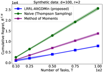
(a) Synthetic data: rank $r=2$

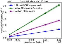
(b) Synthetic data: rank $r=4$

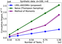
(c) Synthetic data: rank $r=8$

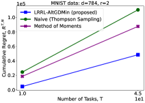
(d) MNIST data: rank $r=2$

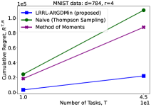
(e) MNIST data: rank $r=4$

(f) MNIST data: rank $r=8$

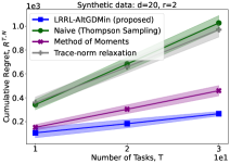
(g) Synthetic data: rank $r=2$

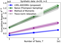
(h) Synthetic data: rank $r=3$

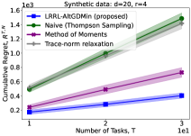
(i) Synthetic data: rank $r=4$

Figure 1: Synthetic data 1: We set the parameters as $d=100$, $K=5$, $N=200$, and noise variance $=10^{-6}$. We considered $M=4$ epochs each with $50$ data samples each. We varied the number of tasks as $T=10,25,50,75,100$. We also varied the rank of the feature matrix as $r=2,4,8$. As shown in the plots (Figures 1(a), 1(b), and 1(c)), our proposed approach outperforms the existing benchmarks. MNIST data: Parameters are $d=784$, $K=2$, $N=5000$, and noise variance $=10^{-6}$. We considered $M=5$ epochs each with $1000$ data samples each. We varied the number of tasks as $T=10,45$. We also varied the rank of the feature matrix as $r=2,4,8$. The plots for MNIST data are presented in Figures 1(d), 1(e), and 1(f). Synthetic data 2: We consider a smaller problem dimension here and also compare with the trace-norm relaxation method. In Figures 1(g), 1(h), and 1(i), we set $d=20$, $K=5$, $N=40$. We considered $M=4$ epochs each with $10$ data samples each, thus $N=40$.

Estimation error. We compared the estimation performance of our proposed LRRL-AltGDMin estimator with three existing approaches: (i) an alternating GD (LRRL-AltGD) estimator, (ii) Method-of-Moments (MoM) based estimator, and (iii) trace-norm convex relaxation-based estimator. The LRRL-AltGD is based on the alternating gradient descent algorithm proposed in (Yi et al., 2016) for solving the low-rank matrix completion problem. LRRL-AltGD alternatively solves for $\widehat{B}$ and $\widehat{W}$ in Eq. (1). The MoM estimator estimates the matrix $\widehat{B}$ using the top-$r$ Singular Value Decomposition (SVD) of $\widehat{\Theta}=\frac{1}{NT}\sum_{{n,t}}y_{{n,t}}^{2}\phi(x_{n,t},c_{n})\phi(x_{n,t},c_{n})^{\top}$. Then, it proceeds to calculate the estimated matrix $\widehat{W}$ through the method of least squares estimator in order to determine the values of $\widehat{\Theta}$. The trace-norm technique relaxes the rank constraint to a trace-norm convex constraint and then iteratively solves for the estimate $\widehat{\Theta}$ and the regularizing parameter $\lambda$. We initialized the LRRL-AltGD algorithm using our proposed spectral initialization approach (Algorithm 2). This is because spectral initialization guarantees a good initialization for solving the nonconvex problem.

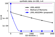
(a) Error vs. GD iteration for epoch-1

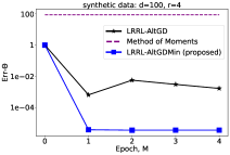
(b) Error vs. Epoch

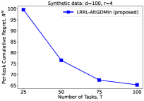
(c) Error vs. Number of tasks

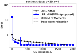
(d) Error vs. GD iteration for epoch-1

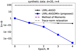
(e) Error vs. Epoch

Figure 2: Synthetic data 1: In Figures 2(a) and 2(b), we set the parameters as $d=100,T=100$, $K=5$, $N=200$, and noise variance $=10^{-6}$. We ran for $L=2000$ GD iterations. We considered $M=4$ epochs each with $50$ data samples each. In Figure 2(c), we separately present the per-task regret vs. number of task plot for $d=100$, $K=5$, $N=100$ (also shown in figure 1(i)) to showcase the sublinear decay. Synthetic data 2: We consider a smaller problem dimension and also compare with the trace-norm relaxation method. In Figures 2(e) and 2(d), we set the parameters as $d=20,T=30$, $K=5$, $N=40$, and noise variance $=10^{-6}$. We ran for $L=2000$ GD iterations. We considered $M=4$ epochs each with $10$ data samples each, thus $N=40$. As expected, the estimation error for our proposed algorithm saturates close to the noise.

We plot the empirical average of $\|\Theta-\Theta^{\star}\|_{F}/\|\Theta^{\star}\|_{F}$ at each iteration $\ell$ (Err-$\Theta$ in the plots) on the y-axis and the iteration by the algorithm until GD iteration $\ell$ on the x-axis. Averaging is over a 100 trials. We note that while LRRL-AltGD, trace-norm, and LRRL-AltGDMin are iterative algorithms, the MoM estimator is non-iterative. To showcase the baselines in our plots, we also show the error achieved by the MoM estimator. Figure 2 presents the error plot. Figure 2(a) presents the Err-$\Theta$ vs. GD iteration for the first epoch. In Figure 2(b), we present the Err-$\Theta$ vs. epoch. We set a total of $5$ epochs, including the zeroth epoch, which is the initialization step. From the plots, we notice that the proposed LRRL-AltGDMin estimator outperforms both the benchmark approaches. Further, the estimation error saturates close to $10^{-6}$. This can be explained using our result, Theorem 5.3, which shows that the error decays exponentially until it reaches the (normalized) “noise-level” ${\sigma_{\eta}}^{2}/\|\theta_{t}^{\star}\|^{2}$, but saturates after that. Although the error in the trace-norm approach improves as the iteration progresses, the improvement is very minimal.

Cumulative regret. We compared the performance of our proposed algorithm against three benchmarks: the Method-of-Moments (MoM)-based representation learning algorithm for bandits in (Yang et al., 2020; Tripuraneni et al., 2021), a Thompson Sampling (TS) algorithm that solves the $T$ tasks separately, and the trace-norm relaxation-based approach in (Cella et al., 2023). As noted, the MoM-based algorithm only estimates the unknown feature matrix $\widehat{\Theta}$ in the first epoch. In subsequent epochs, this $\widehat{\Theta}$ is consistently used to choose actions. On the other hand, the naive approach implements the TS method separately to determine the estimate of $\theta_{t}^{\star}$ for each task $t\in[T]$. The approach in (Cella et al., 2023) considered a trace-norm convex relaxation of the original non-convex cost function (Eqs. (4) and (11) in (Cella et al., 2023)). Figure 1 presents the cumulative regret plots for the different algorithms. We varied the number of tasks and the rank of the feature matrix and compared the results of our proposed algorithm with the MoM-based, trace-norm relaxation, and TS-based algorithms. Our plot demonstrates that as the number of tasks increases, the advantage of the proposed LRRL-AltGDMin algorithm increases compared to the naive approach, the MoM, and the trace-norm relaxation approaches. We varied the rank $r$ and compared the performances. The performance of the TS algorithm is unaltered by varying the rank. This is expected since the regret of the TS algorithm does not depend on the rank. In all experiments, our algorithm consistently outperforms the benchmarks, validating its effectiveness.

7 Conclusion and Future Work

In this work, we introduced an alternating gradient descent and minimization algorithm for multi-task representation learning in linear contextual bandits. Leveraging this estimator, we developed a bandit algorithm and established its regret bound for low dimensional contextual bandits. Our approach consistently outperformed existing methods in numerical experiments. Inspired by (Hu et al., 2021), as part of our future work, we plan to extend our algorithm to an upper confidence bound-based approach by computing the confidence interval. Further, one of the very interesting future directions is to relax the i.i.d standard Gaussian assumption on the feature vectors. While this assumption holds for the initial epoch during the random exploration, it becomes restrictive when we perform greedy exploration in subsequent epochs. As part of our future work, we intend to explore methods for relaxing the i.i.d assumption for epochs after the first one. One potential direction is to fix the $B$ estimate and solve only for $W$ after epoch one, similar to few-shot learning and online subspace tracking (Babu et al., 2023).

Impact Statement

This paper presents work whose goal is to advance the field of Machine Learning. There are many potential societal consequences of our work, none which we feel must be specifically highlighted here.

Appendix A Preliminaries

Proposition A.1 (Theorem 2.8.1, (Vershynin, 2018)).

Let $X_{1},\cdots,X_{N}$ be independent, mean zero, sub-exponential random variables. Then, for every $g\geqslant 0$, we have

$$\mathbb{P}\Bigl{\{}|\sum_{i=1}^{N}X_{i}\geqslant g|\Bigl{\}}\leqslant 2\exp\left[-c\min\left(\frac{g^{2}}{\sum_{i=1}^{N}\left\lVert X_{i}\right\rVert_{\psi_{1}}^{2}},\frac{g}{\max_{i}\left\lVert X_{i}\right\rVert_{\psi_{1}}}\right)\right],$$

where $c>0$ is an absolute constant.

Proposition A.2 (Chernoff bound for Gaussian).

Let $X\sim\pazocal{N}(\mu_{x},\sigma_{x}^{2})$, then

$$\mathbb{P}\Bigl{\{}X-\mu_{x}\geqslant g\Bigl{\}}\leqslant\exp(-\frac{g^{2}}{2\sigma_{x}^{2}}).$$

Appendix B Guarantees for LRRL-AltGDMin Estimator

Define

$$G :=B^{\top}\Theta^{\star}$$

$$P :=I-B^{\star}{B^{\star}}^{\top}$$

$$\mathrm{GradB} :=\nabla_{B}f(B,W)=\sum_{t=1}^{T}\Phi_{t}^{{\scalebox{0.6}{(m)}}}(\Phi_{t}^{{\scalebox{0.6}{(m)}}}Bw_{k}-Y_{t}^{{\scalebox{0.6}{(m)}}})w_{k}^{\top}$$

$$=\sum_{t=1}^{T}\sum_{n={\pazocal{G}}_{m-1}}^{{\pazocal{G}}_{m}}(y_{n,t}-\phi(x_{n,t},c_{n})^{\top}Bw_{t})\phi(x_{n,t},c_{n})w_{t}^{\top}$$

$$=\sum_{t=1}^{T}\sum_{n={\pazocal{G}}_{m-1}}^{{\pazocal{G}}_{m}}\phi(x_{n,t},c_{n})\phi(x_{n,t},c_{n})^{\top}(\theta_{t}-\theta_{t}^{\star})w_{t}^{\top}+\eta_{n,t}\phi(x_{n,t},c_{n})w_{t}^{\top}$$

$$\mathrm{GradB}^{\prime} =\sum_{t=1}^{T}\sum_{n={\pazocal{G}}_{m-1}}^{{\pazocal{G}}_{m}}\phi(x_{n,t},c_{n})\phi(x_{n,t},c_{n})^{\top}(\theta_{t}^{\star}-\theta_{t})w_{t}^{\top}.$$

and $g_{t}=B^{\top}\theta_{t}^{\star}$ for all $t\in[T]$, $\mathrm{SD}(B_{1},B_{2})=\|(I-B_{1}B_{1}^{\top})B_{2}\|_{F}$ as the Subspace Distance (SD) measure for basis matrices $B_{1},B_{2}$. Here, $\mathrm{GradB}$ represents the gradient that includes noise, while $\mathrm{GradB}^{\prime}$ represents the gradient without noise.

Proposition B.1.

Assume $\mathrm{SD}(B,B^{\star})\leqslant\delta_{\ell}$. Then, with probability at least $1-2T\exp(r-c({\pazocal{G}}_{m}-{\pazocal{G}}_{m-1}))$, it holds that

$$\|M^{-1}\|\leqslant\frac{1}{0.9({\pazocal{G}}_{m}-{\pazocal{G}}_{m-1})}\quad\text{and}\quad\|M^{-1}B^{\top}{\Phi_{t}^{{\scalebox{0.6}{(m)}}}}^{\top}{\Phi_{t}^{{\scalebox{0.6}{(m)}}}}(I-BB^{\top})\theta_{t}^{\star}\|\leqslant 0.12\delta_{\ell}\|w_{t}^{\star}\|,$$

where $M=B^{\top}{\Phi_{t}^{{\scalebox{0.6}{(m)}}}}^{\top}{\Phi_{t}^{{\scalebox{0.6}{(m)}}}}B$.

Proof.

To demonstrate the upper bound of $\|M^{-1}\|$, let’s consider a fixed $z\in{\pazocal{S}}_{r}$. We then have

$$z^{\top}B^{\top}{\Phi_{t}^{{\scalebox{0.6}{(m)}}}}^{\top}{\Phi_{t}^{{\scalebox{0.6}{(m)}}}}Bz=\sum_{n={\pazocal{G}}_{m-1}}^{{\pazocal{G}}_{m}}z^{\top}B^{\top}\phi(x_{n,t},c_{n})\phi(x_{n,t},c_{n})^{\top}Bz.$$

Furthermore, we find that

$$\mathbb{E}[\langle B^{\top}\phi(x_{n,t},c_{n}),z\rangle^{2}]=\mathbb{E}[z^{\top}B^{\top}\phi(x_{n,t},c_{n})\phi(x_{n,t},c_{n})^{\top}Bz]=z^{\top}B^{\top}\mathbb{E}[\phi(x_{n,t},c_{n})\phi(x_{n,t},c_{n})^{\top}]Bz=1,$$

and also

$$\mathbb{E}[z^{\top}B^{\top}\phi(x_{n,t},c_{n})] =0$$

$$\mathrm{Var}[z^{\top}B^{\top}\phi(x_{n,t},c_{n})] =\mathbb{E}[z^{\top}B^{\top}\phi(x_{n,t},c_{n})]^{2}$$

$$=\mathbb{E}[z^{\top}B^{\top}\phi(x_{n,t},c_{n})\phi(x_{n,t},c_{n})^{\top}Bz]$$

$$=z^{\top}B^{\top}\mathbb{E}[\phi(x_{n,t},c_{n})\phi(x_{n,t},c_{n})^{\top}]Bz$$

$$=1.$$

The summands are independent sub-exponential random variables with norm $K_{n}\leqslant 1$. We apply the sub-exponential Bernstein inequality stated in Proposition A.1 by setting $g=\epsilon_{2}({\pazocal{G}}_{m}-{\pazocal{G}}_{m-1})$. In order to implement this, we show that

$$\frac{g^{2}}{\sum_{n={\pazocal{G}}_{m-1}}^{{\pazocal{G}}_{m}}K_{n}^{2}} \geqslant\frac{\epsilon_{2}^{2}({\pazocal{G}}_{m}-{\pazocal{G}}_{m-1})^{2}}{({\pazocal{G}}_{m}-{\pazocal{G}}_{m-1})}=\epsilon_{2}^{2}({\pazocal{G}}_{m}-{\pazocal{G}}_{m-1})$$

$$\frac{g}{\max_{n}K_{n}} \geqslant\frac{\epsilon_{2}({\pazocal{G}}_{m}-{\pazocal{G}}_{m-1})}{\max_{n}1}=\epsilon_{2}({\pazocal{G}}_{m}-{\pazocal{G}}_{m-1})$$

Therefore, for a fixed $z\in{\pazocal{S}}_{r}$, with probability at least $1-\exp(-c\epsilon_{2}^{2}({\pazocal{G}}_{m}-{\pazocal{G}}_{m-1}))$,

$$z^{\top}B^{\top}{\Phi_{t}^{{\scalebox{0.6}{(m)}}}}^{\top}{\Phi_{t}^{{\scalebox{0.6}{(m)}}}}Bz-({\pazocal{G}}_{m}-{\pazocal{G}}_{m-1})I\geqslant-\epsilon_{2}({\pazocal{G}}_{m}-{\pazocal{G}}_{m-1}).$$

Using epsilon-net over all $z\in{\pazocal{S}}_{r}$ adds a factor of $\exp(r)$. Thus, with probability at least $1-\exp(r-c\epsilon_{2}^{2}({\pazocal{G}}_{m}-{\pazocal{G}}_{m-1}))$, we have $\min_{z\in{\pazocal{S}}_{r}}\sum_{n={\pazocal{G}}_{m-1}}^{{\pazocal{G}}_{m}}z^{\top}B^{\top}\phi(x_{n,t},c_{n})\phi(x_{n,t},c_{n})^{\top}Bz\geqslant(1-\epsilon_{2})({\pazocal{G}}_{m}-{\pazocal{G}}_{m-1})$. Setting $\epsilon_{2}=0.1$, we obtain

$$\|M^{-1}\| =\|(B^{\top}{\Phi_{t}^{{\scalebox{0.6}{(m)}}}}^{\top}{\Phi_{t}^{{\scalebox{0.6}{(m)}}}}B)^{-1}\|$$

$$=\frac{1}{\sigma_{\min}(B^{\top}{\Phi_{t}^{{\scalebox{0.6}{(m)}}}}^{\top}{\Phi_{t}^{{\scalebox{0.6}{(m)}}}}B)}$$

$$=\frac{1}{\min_{z\in{\pazocal{S}}_{r}}\sum_{n={\pazocal{G}}_{m-1}}^{{\pazocal{G}}_{m}}\langle B^{\top}\phi(x_{n,t},c_{n}),z\rangle^{2}}$$

$$\leqslant\frac{1}{0.9({\pazocal{G}}_{m}-{\pazocal{G}}_{m-1})}.$$

To demonstrate the upper bound of $\|M^{-1}B^{\top}{\Phi_{t}^{{\scalebox{0.6}{(m)}}}}^{\top}{\Phi_{t}^{{\scalebox{0.6}{(m)}}}}(I-BB^{\top})\theta_{t}^{\star}\|$, it is necessary to first determine the upper bound of $\|B^{\top}{\Phi_{t}^{{\scalebox{0.6}{(m)}}}}^{\top}{\Phi_{t}^{{\scalebox{0.6}{(m)}}}}(I-BB^{\top})\theta_{t}^{\star}\|$. Consider a fixed $z\in{\pazocal{S}}_{r}$, we have

$$z^{\top}B^{\top}{\Phi_{t}^{{\scalebox{0.6}{(m)}}}}^{\top}{\Phi_{t}^{{\scalebox{0.6}{(m)}}}}(I-BB^{\top})\theta_{t}^{\star}=\sum_{n={\pazocal{G}}_{m-1}}^{{\pazocal{G}}_{m}}(\phi(x_{n,t},c_{n})^{\top}Bz)^{\top}(\phi(x_{n,t},c_{n})^{\top}(I-BB^{\top})\theta_{t}^{\star}).$$

Furthermore, we find that

$$\mathbb{E}[(\phi(x_{n,t},c_{n})^{\top}Bz)^{\top}(\phi(x_{n,t},c_{n})^{\top}(I-BB^{\top})\theta_{t}^{\star})] =z^{\top}B^{\top}\mathbb{E}[\phi(x_{n,t},c_{n})\phi(x_{n,t},c_{n})^{\top}](I-BB^{\top})\theta_{t}^{\star}$$

$$=z^{\top}B^{\top}(I-BB^{\top})\theta_{t}^{\star}$$

$$=0,$$

and also we have

$$\mathbb{E}[(\phi(x_{n,t},c_{n})^{\top}Bz)^{\top}] =0$$

$$\mathrm{Var}((\phi(x_{n,t},c_{n})^{\top}Bz)^{\top}) =\mathbb{E}[(\phi(x_{n,t},c_{n})^{\top}Bz)^{\top}]^{2}$$

$$=\mathbb{E}[z^{\top}B^{\top}\phi(x_{n,t},c_{n})\phi(x_{n,t},c_{n})^{\top}Bz]$$

$$=z^{\top}B^{\top}\mathbb{E}[\phi(x_{n,t},c_{n})\phi(x_{n,t},c_{n})^{\top}]Bz$$

$$=1$$

and

$$\mathbb{E}[\phi(x_{n,t},c_{n})^{\top}(I-BB^{\top})\theta_{t}^{\star}] =0$$

$$\mathrm{Var}(\phi(x_{n,t},c_{n})^{\top}(I-BB^{\top})\theta_{t}^{\star}) =\mathbb{E}[\phi(x_{n,t},c_{n})^{\top}(I-BB^{\top})\theta_{t}^{\star}]^{2}$$

$$=\mathbb{E}[{\theta_{t}^{\star}}^{\top}(I-BB^{\top})^{\top}\phi(x_{n,t},c_{n})\phi(x_{n,t},c_{n})^{\top}(I-BB^{\top})\theta_{t}^{\star}]$$

$$={\theta_{t}^{\star}}^{\top}(I-BB^{\top})^{\top}\mathbb{E}[\phi(x_{n,t},c_{n})\phi(x_{n,t},c_{n})^{\top}](I-BB^{\top})\theta_{t}^{\star}$$

$$=\|(I-BB^{\top})\theta_{t}^{\star}\|^{2}$$

The summands are independent sub-exponential random variables with norm $K_{n}\leqslant\|(I-BB^{\top})\theta_{t}^{\star}\|$. We apply the sub-exponential Bernstein inequality stated in Proposition A.1 by setting $g=\epsilon_{3}({\pazocal{G}}_{m}-{\pazocal{G}}_{m-1})\|(I-BB^{\top})\theta_{t}^{\star}\|$. In order to implement this, we show that

$$\frac{g^{2}}{\sum_{n={\pazocal{G}}_{m-1}}^{{\pazocal{G}}_{m}}K_{n}^{2}} \geqslant\frac{\epsilon_{3}^{2}({\pazocal{G}}_{m}-{\pazocal{G}}_{m-1})^{2}\|(I-BB^{\top})\theta_{t}^{\star}\|^{2}}{({\pazocal{G}}_{m}-{\pazocal{G}}_{m-1})\|(I-BB^{\top})\theta_{t}^{\star}\|^{2}}=\epsilon_{3}^{2}({\pazocal{G}}_{m}-{\pazocal{G}}_{m-1})$$

$$\frac{g}{\max_{n}K_{n}} \geqslant\frac{\epsilon_{3}({\pazocal{G}}_{m}-{\pazocal{G}}_{m-1})\|(I-BB^{\top})\theta_{t}^{\star}\|}{\max_{n}\|(I-BB^{\top})\theta_{t}^{\star}\|}=\epsilon_{3}({\pazocal{G}}_{m}-{\pazocal{G}}_{m-1})$$

Therefore, for a fixed $z\in{\pazocal{S}}_{r}$, with probability at least $1-\exp(-c\epsilon_{3}^{2}({\pazocal{G}}_{m}-{\pazocal{G}}_{m-1}))$,

$$z^{\top}B^{\top}{\Phi_{t}^{{\scalebox{0.6}{(m)}}}}^{\top}{\Phi_{t}^{{\scalebox{0.6}{(m)}}}}Bz\leqslant\epsilon_{3}({\pazocal{G}}_{m}-{\pazocal{G}}_{m-1})\|(I-BB^{\top})\theta_{t}^{\star}\|.$$

Using epsilon-net over all $z\in{\pazocal{S}}_{r}$ adds a factor of $\exp(r)$. Thus, with probability at least $1-\exp(r-c\epsilon_{3}^{2}({\pazocal{G}}_{m}-{\pazocal{G}}_{m-1}))$, we have $\max_{z\in{\pazocal{S}}_{r}}\sum_{n={\pazocal{G}}_{m-1}}^{{\pazocal{G}}_{m}}(\phi(x_{n,t},c_{n})^{\top}Bz)^{\top}(\phi(x_{n,t},c_{n})^{\top}(I-BB^{\top})\theta_{t}^{\star})\leqslant\epsilon_{3}({\pazocal{G}}_{m}-{\pazocal{G}}_{m-1})\|(I-BB^{\top})\theta_{t}^{\star}\|$. Therefore, we have

$$\|B^{\top}{\Phi_{t}^{{\scalebox{0.6}{(m)}}}}^{\top}{\Phi_{t}^{{\scalebox{0.6}{(m)}}}}(I-BB^{\top})\theta_{t}^{\star}\| =\max_{z\in{\pazocal{S}}_{r}}z^{\top}B^{\top}\phi(x_{n,t},c_{n})^{\top}\phi(x_{n,t},c_{n})(I-BB^{\top})\theta_{t}^{\star}$$

$$=\max_{z\in{\pazocal{S}}_{r}}\sum_{n={\pazocal{G}}_{m-1}}^{{\pazocal{G}}_{m}}(\phi(x_{n,t},c_{n})^{\top}Bz)^{\top}(\phi(x_{n,t},c_{n})^{\top}(I-BB^{\top})\theta_{t}^{\star})$$

$$\leqslant\epsilon_{3}({\pazocal{G}}_{m}-{\pazocal{G}}_{m-1})\|(I-BB^{\top})\theta_{t}^{\star}\|$$

By combining these results, using a union bound over all $T$ vectors, and setting $\epsilon_{3}=0.1$, we conclude that with probability at least $1-2T\exp(r-c({\pazocal{G}}_{m}-{\pazocal{G}}_{m-1}))$,

$$\|M^{-1}B^{\top}{\Phi_{t}^{{\scalebox{0.6}{(m)}}}}^{\top}{\Phi_{t}^{{\scalebox{0.6}{(m)}}}}(I-BB^{\top})\theta_{t}^{\star}\| \leqslant\|M^{-1}\|\times\|B^{\top}{\Phi_{t}^{{\scalebox{0.6}{(m)}}}}^{\top}{\Phi_{t}^{{\scalebox{0.6}{(m)}}}}(I-BB^{\top})\theta_{t}^{\star}\|$$

$$\leqslant\frac{1}{0.9({\pazocal{G}}_{m}-{\pazocal{G}}_{m-1})}\epsilon_{3}({\pazocal{G}}_{m}-{\pazocal{G}}_{m-1})\|(I-BB^{\top})\theta_{t}^{\star}\|$$

$$\leqslant 0.12\|(I-BB^{\top})\theta_{t}^{\star}\|$$

$$\leqslant 0.12\delta_{\ell}\|w_{t}^{\star}\|.$$

∎

Lemma B.2.

Assume $\sigma_{\eta}^{2}\leqslant\frac{r}{T}\delta_{\ell}^{2}{\sigma_{\max}^{\star}}^{2}$, and $\mathrm{SD}(B,B^{\star})\leqslant\delta_{\ell}$, if $\delta_{\ell}\leqslant\frac{0.02}{\mu\sqrt{r}\kappa^{2}}$, and if $({\pazocal{G}}_{m}-{\pazocal{G}}_{m-1})\geqslant C\max(\log T,\log d,r)$, then with probability at least $1-3\exp(\log T+r-c({\pazocal{G}}_{m}-{\pazocal{G}}_{m-1}))$, the following bounds hold:

1. $\|w_{t}-g_{t}\|\leqslant 0.24\mu\delta_{\ell}\sqrt{\frac{r}{T}}\sigma_{\max}^{\star}$

2. $\|w_{t}\|\leqslant 1.24\mu\sqrt{\frac{r}{T}}\sigma_{\max}^{\star}$

3. $\|W-G\|_{F}\leqslant 0.24\mu\delta_{\ell}\sqrt{r}\sigma_{\max}^{\star}$

4. $\|\theta_{t}-\theta_{t}^{\star}\|\leqslant 1.24\mu\delta_{\ell}\sqrt{\frac{r}{T}}\sigma_{\max}^{\star}$

5. $\|\Theta_{l}-\Theta^{\star}\|_{F}\leqslant 1.24\mu\delta_{\ell}\sqrt{r}\sigma_{\max}^{\star}$

6. $\sigma_{\min}(W)\geqslant 0.9\sigma_{\min}^{\star}$

7. $\sigma_{\max}(W)\leqslant 1.1{\sigma_{\max}^{\star}}$

Proof.

Consider the expression for $w_{t}$, we obtain that

$$w_{t} =(\Phi_{t}^{{\scalebox{0.6}{(m)}}}B)^{\dagger}Y_{t}^{{\scalebox{0.6}{(m)}}}$$

$$=((\Phi_{t}^{{\scalebox{0.6}{(m)}}}B)^{\top}(\Phi_{t}^{{\scalebox{0.6}{(m)}}}B))^{-1}(\Phi_{t}^{{\scalebox{0.6}{(m)}}}B)^{\top}Y_{t}^{{\scalebox{0.6}{(m)}}}$$

$$=(B^{\top}{\Phi_{t}^{{\scalebox{0.6}{(m)}}}}^{\top}\Phi_{t}^{{\scalebox{0.6}{(m)}}}B)^{-1}B^{\top}{\Phi_{t}^{{\scalebox{0.6}{(m)}}}}^{\top}Y_{t}^{{\scalebox{0.6}{(m)}}}$$

$$=(B^{\top}{\Phi_{t}^{{\scalebox{0.6}{(m)}}}}^{\top}\Phi_{t}^{{\scalebox{0.6}{(m)}}}B)^{-1}(B^{\top}{\Phi_{t}^{{\scalebox{0.6}{(m)}}}}^{\top})\Phi_{t}^{{\scalebox{0.6}{(m)}}}BB^{\top}\theta_{t}^{\star}+(B^{\top}{\Phi_{t}^{{\scalebox{0.6}{(m)}}}}^{\top}\Phi_{t}^{{\scalebox{0.6}{(m)}}}B)^{-1}(B^{\top}{\Phi_{t}^{{\scalebox{0.6}{(m)}}}}^{\top})\Phi_{t}^{{\scalebox{0.6}{(m)}}}(I-BB^{\top})\theta_{t}^{\star}$$

$$+(B^{\top}{\Phi_{t}^{{\scalebox{0.6}{(m)}}}}^{\top}\Phi_{t}^{{\scalebox{0.6}{(m)}}}B)^{-1}(B^{\top}{\Phi_{t}^{{\scalebox{0.6}{(m)}}}}^{\top})\eta_{t}^{{\scalebox{0.6}{(m)}}}$$

$$=(B^{\top}{\Phi_{t}^{{\scalebox{0.6}{(m)}}}}^{\top}\Phi_{t}^{{\scalebox{0.6}{(m)}}}B)^{-1}(B^{\top}{\Phi_{t}^{{\scalebox{0.6}{(m)}}}}^{\top}\Phi_{t}^{{\scalebox{0.6}{(m)}}}B)B^{\top}\theta_{t}^{\star}+(B^{\top}{\Phi_{t}^{{\scalebox{0.6}{(m)}}}}^{\top}\Phi_{t}^{{\scalebox{0.6}{(m)}}}B)^{-1}(B^{\top}{\Phi_{t}^{{\scalebox{0.6}{(m)}}}}^{\top})\Phi_{t}^{{\scalebox{0.6}{(m)}}}(I-BB^{\top})\theta_{t}^{\star}$$

$$+(B^{\top}{\Phi_{t}^{{\scalebox{0.6}{(m)}}}}^{\top}\Phi_{t}^{{\scalebox{0.6}{(m)}}}B)^{-1}(B^{\top}{\Phi_{t}^{{\scalebox{0.6}{(m)}}}}^{\top})\eta_{t}^{{\scalebox{0.6}{(m)}}}$$

$$=g_{t}+M^{-1}B^{\top}{\Phi_{t}^{{\scalebox{0.6}{(m)}}}}^{\top}\Phi_{t}^{{\scalebox{0.6}{(m)}}}(I-BB^{\top})\theta_{t}^{\star}+M^{-1}B^{\top}{\Phi_{t}^{{\scalebox{0.6}{(m)}}}}^{\top}\eta_{t}^{{\scalebox{0.6}{(m)}}},$$

where $M=B^{\top}{\Phi_{t}^{{\scalebox{0.6}{(m)}}}}^{\top}\Phi_{t}^{{\scalebox{0.6}{(m)}}}B$. Consequently, $w_{t}-g_{t}=M^{-1}B^{\top}{\Phi_{t}^{{\scalebox{0.6}{(m)}}}}^{\top}\Phi_{t}^{{\scalebox{0.6}{(m)}}}(I-BB^{\top})\theta_{t}^{\star}+M^{-1}B^{\top}{\Phi_{t}^{{\scalebox{0.6}{(m)}}}}^{\top}\eta_{t}^{{\scalebox{0.6}{(m)}}}$. The first term is bounded in Proposition B.1. To bound the second term, let’s consider a fixed $z\in{\pazocal{S}}_{r}$. We analyze $z^{\top}B^{\top}{\Phi_{t}^{{\scalebox{0.6}{(m)}}}}^{\top}\eta_{t}^{{\scalebox{0.6}{(m)}}}=\sum_{n={\pazocal{G}}_{m-1}+1}^{{\pazocal{G}}_{m}}(Bz)^{\top}\phi(x_{n,t},c_{n})\eta_{n,t}$, leading to $\mathbb{E}[(Bz)^{\top}\phi(x_{n,t},c_{n})\eta_{n,t}]=0$ and

$$\mathrm{Var}((Bz)^{\top}\phi(x_{n,t},c_{n})) =\mathbb{E}[(Bz)^{\top}\phi(x_{n,t},c_{n})]^{2}-(\mathbb{E}[(Bz)^{\top}\phi(x_{n,t},c_{n})])^{2}$$

$$=\mathbb{E}[(Bz)^{\top}\phi(x_{n,t},c_{n})]^{2}$$

$$=\mathbb{E}[z^{\top}B^{\top}\phi(x_{n,t},c_{n})\phi(x_{n,t},c_{n})^{\top}Bz]$$

$$=z^{\top}B^{\top}\mathbb{E}[\phi(x_{n,t},c_{n})\phi(x_{n,t},c_{n})^{\top}]Bz$$

$$=z^{\top}B^{\top}Bz$$

$$=I.$$

Given $\eta_{n,t}\stackrel{{\scriptstyle\mathrm{iid}}}{{\thicksim}}{\cal{N}}(0,\sigma_{\eta}^{2})$, we have $\mathrm{Var}(\eta_{n,t})=\sigma_{\eta}^{2}$. Thus, $z^{\top}B^{\top}{\Phi_{t}^{{\scalebox{0.6}{(m)}}}}^{\top}\eta_{t}^{{\scalebox{0.6}{(m)}}}$ is a sum of $({\pazocal{G}}_{m}-{\pazocal{G}}_{m-1})$ subexponential random variables with parameter $K_{n}=\sigma_{\eta}$. We apply the sub-exponential Bernstein inequality stated in Proposition A.1 by setting $g=\epsilon_{3}({\pazocal{G}}_{m}-{\pazocal{G}}_{m-1})\sigma_{\eta}$. In order to implement this, we show that

$$\frac{g^{2}}{\sum_{n={\pazocal{G}}_{m-1}+1}^{{\pazocal{G}}_{m}}K_{n}^{2}} \geqslant\frac{\epsilon_{3}^{2}({\pazocal{G}}_{m}-{\pazocal{G}}_{m-1})^{2}\sigma_{\eta}^{2}}{({\pazocal{G}}_{m}-{\pazocal{G}}_{m-1})\sigma_{\eta}^{2}}=\epsilon_{3}^{2}({\pazocal{G}}_{m}-{\pazocal{G}}_{m-1})$$

$$\frac{g}{\max_{n}K_{n}} \geqslant\frac{\epsilon_{3}({\pazocal{G}}_{m}-{\pazocal{G}}_{m-1})\sigma_{\eta}}{\sigma_{\eta}}=\epsilon_{3}({\pazocal{G}}_{m}-{\pazocal{G}}_{m-1})$$

Therefore, for a fixed $z\in{\pazocal{S}}_{r}$, with probability at least $1-\exp(-c\epsilon_{3}^{2}({\pazocal{G}}_{m}-{\pazocal{G}}_{m-1}))$, $z^{\top}B^{\top}{\Phi_{t}^{{\scalebox{0.6}{(m)}}}}^{\top}\eta_{t}^{{\scalebox{0.6}{(m)}}}\leqslant\epsilon_{3}({\pazocal{G}}_{m}-{\pazocal{G}}_{m-1})\sigma_{\eta}$. Using epsilon-net over all $z$ adds a factor of $\exp(r)$. Thus, with probability at least $1-\exp(r-c\epsilon_{3}^{2}({\pazocal{G}}_{m}-{\pazocal{G}}_{m-1})\sigma_{\eta})$, we have $B^{\top}{\Phi_{t}^{{\scalebox{0.6}{(m)}}}}^{\top}\eta_{t}^{{\scalebox{0.6}{(m)}}}\leqslant\epsilon_{3}({\pazocal{G}}_{m}-{\pazocal{G}}_{m-1})\sigma_{\eta}$. Then, the above holds for all $t\in[T]$ with probability at least $1-\exp(\log T+r-c\epsilon_{3}^{2}({\pazocal{G}}_{m}-{\pazocal{G}}_{m-1}))$. According to Proposition B.1, with probability at least $1-2T\exp(r-c({\pazocal{G}}_{m}-{\pazocal{G}}_{m-1}))$, we have $\|M^{-1}\|\leqslant\frac{1}{0.9({\pazocal{G}}_{m}-{\pazocal{G}}_{m-1})}$. Combining these results, it follows that with probability at least $1-2T\exp(r-c({\pazocal{G}}_{m}-{\pazocal{G}}_{m-1}))$, $\|M^{-1}B^{\top}{\Phi_{t}^{{\scalebox{0.6}{(m)}}}}^{\top}\eta_{t}^{{\scalebox{0.6}{(m)}}}\|\leqslant\frac{\sigma_{\eta}}{9}$. Combining with bound on the first term, we then determine that with probability at least $1-3\exp(\log T+r-c({\pazocal{G}}_{m}-{\pazocal{G}}_{m-1}))$,

$$\|w_{t}-g_{t}\|\leqslant 0.12\delta_{\ell}\|w_{t}^{\star}\|+\frac{\sigma_{\eta}}{9}.$$

Given that $\sigma_{\eta}\leqslant\sqrt{\frac{r}{T}}\delta_{\ell}\sigma_{\max}^{\star}$, we then have

$$\|w_{t}-g_{t}\|\leqslant 0.24\delta_{\ell}\max(\|w_{t}^{\star}\|,\sqrt{\frac{r}{T}}\sigma_{\max}^{\star}).$$

Applying the Incoherence of right singular vectors in Assumption 2.2, we have

$$\|w_{t}-g_{t}\| \leqslant 0.24\delta_{\ell}\max(\mu\sqrt{\frac{r}{T}}{\sigma_{\max}^{\star}},\sqrt{\frac{r}{T}}\sigma_{\max}^{\star})\leqslant 0.24\mu\delta_{\ell}\sqrt{\frac{r}{T}}\sigma_{\max}^{\star}.$$ (2)

This proves 1).

Eq. (2) implies

$$\|W-G\|_{F}\leqslant 0.24\mu\delta_{\ell}\sqrt{r}\sigma_{\max}^{\star}.$$

This completes the proof of 3).

To bound $\|w_{t}\|$, we use $\|g_{t}\|\leqslant\|w_{t}^{\star}\|$, and then find

$$\|w_{t}\| =\|w_{t}-g_{t}+g_{t}\|$$

$$\leqslant\|w_{t}-g_{t}\|+\|w_{t}^{\star}\|$$

$$\leqslant 0.24\mu\delta_{\ell}\sqrt{\frac{r}{T}}\sigma_{\max}^{\star}+\mu\sqrt{\frac{r}{T}}\sigma_{\max}^{\star}$$

$$\leqslant 1.24\mu\sqrt{\frac{r}{T}}\sigma_{\max}^{\star}.$$

This completes the proof of 2).

For $\|\theta_{t}-\theta_{t}^{\star}\|$, we derive

$$\|\theta_{t}-\theta_{t}^{\star}\| =\|Bg_{t}+(I-BB^{\top})\theta_{t}^{\star}-Bw_{t}\|$$

$$=\|B(g_{t}-w_{t})+(I-BB^{\top})\theta_{t}^{\star}\|$$

$$\leqslant\|g_{t}-w_{t}\|+\|(I-BB^{\top})B^{\star}w_{t}^{\star}\|$$

$$\leqslant 0.24\mu\delta_{\ell}\sqrt{\frac{r}{T}}\sigma_{\max}^{\star}+\mu\delta_{\ell}\sqrt{\frac{r}{T}}\sigma_{\max}^{\star}$$

$$\leqslant 1.24\mu\delta_{\ell}\sqrt{\frac{r}{T}}\sigma_{\max}^{\star}.$$

This implies that

$$\|\Theta_{l}-\Theta^{\star}\|_{F}\leqslant 1.24\mu\delta_{\ell}\sqrt{r}\sigma_{\max}^{\star}.$$

This proves 4) and 5).

Furthermore,

$$\sigma_{\min}(W) =\sigma_{\min}(G-(G-W))$$

$$\geqslant\sigma_{\min}(G)-\|W-G\|$$

$$\geqslant\sigma_{\min}(G)-\|W-G\|_{F}$$

we have

$$\sigma_{\min}(G) =\sigma_{\min}(G^{\top})$$

$$=\sigma_{\min}({W^{\star}}^{\top}{B^{\star}}^{\top}B)$$

$$\geqslant\sigma_{\min}^{\star}\sigma_{\min}({B^{\star}}^{\top}B),$$

and

$$\sigma_{\min}({B^{\star}}^{\top}B) =\sqrt{\lambda_{\min}(B^{\top}B^{\star}{B^{\star}}^{\top}B)})$$

$$=\sqrt{\lambda_{\min}(B^{\top}(I-P)B)}$$

$$=\sqrt{\lambda_{\min}(I-B^{\top}PB)}$$

$$=\sqrt{\lambda_{\min}(I-B^{\top}P^{2}B)}$$

$$=\sqrt{1-\lambda_{\max}(B^{\top}P^{2}B)}$$

$$=\sqrt{1-\|PB\|^{2}}$$

$$\geqslant\sqrt{1-\delta_{\ell}^{2}}.$$

Combining the above three bounds, if $\delta_{\ell}<\frac{0.02}{\mu\sqrt{r}\kappa^{2}}$, we then have

$$\sigma_{\min}(W)\geqslant\sqrt{1-\delta_{\ell}^{2}}\sigma_{\min}^{\star}-0.24\mu\delta_{\ell}\sqrt{r}\sigma_{\max}^{\star}\geqslant 0.9\sigma_{\min}^{\star}$$

and

$$\sigma_{\max}(W) =\sigma_{\max}(G-(G-W))$$

$$\leqslant\sigma_{\max}(G)+\sigma_{\max}(G-W)$$

$$=\sigma_{\max}(B^{\top}B^{\star}W^{\star})+\sigma_{\max}(G-W)$$

$$\leqslant\sigma_{\max}(B^{\top}B^{\star})\sigma_{\max}(W^{\star})+\|G-W\|_{F}$$

$$\leqslant\sigma_{\max}^{\star}+0.24\mu\delta_{\ell}\sqrt{r}\sigma_{\max}^{\star}$$

$$=1.1{\sigma_{\max}^{\star}}$$

Thus, the proof is complete. ∎

Proposition B.3.

Assume $\mathrm{SD}(B,B^{\star})\leqslant\delta_{\ell}$. The following statements are true:

• $\mathbb{E}[\mathrm{GradB}^{\prime}]=({\pazocal{G}}_{m}-{\pazocal{G}}_{m-1})(\Theta^{\star}-\Theta)W^{\top}$

• With probability at least $1-3T\exp(r-c({\pazocal{G}}_{m}-{\pazocal{G}}_{m-1}))$, we have $\|\mathbb{E}[\mathrm{GradB}^{\prime}]\|\leqslant 1.37({\pazocal{G}}_{m}-{\pazocal{G}}_{m-1})\mu\delta_{\ell}\sqrt{r}{\sigma_{\max}^{\star}}^{2}$

• If $\delta_{\ell}\leqslant\frac{0.02}{\mu\sqrt{r}\kappa^{2}}$, then, with probability at least $1-\exp(C(d+r)-c\frac{\epsilon_{1}^{2}({\pazocal{G}}_{m}-{\pazocal{G}}_{m-1})T}{\mu^{2}r\kappa^{4}})-3\exp(\log T+r-c({\pazocal{G}}_{m}-{\pazocal{G}}_{m-1}))$, the inequality $\|\mathrm{GradB}^{\prime}-\mathbb{E}[\mathrm{GradB}^{\prime}]\|\leqslant\epsilon_{1}\delta_{\ell}({\pazocal{G}}_{m}-{\pazocal{G}}_{m-1}){\sigma_{\min}^{\star}}^{2}$ holds

where $\mathrm{GradB}^{\prime}=\sum_{t=1,n={\pazocal{G}}_{m-1}+1}^{T,{\pazocal{G}}_{m}}\phi(x_{n,t},c_{n})\phi(x_{n,t},c_{n})^{\top}(\theta_{t}^{\star}-\theta_{t})w_{t}^{\top}$.

Proof.

By using independence of $\Phi_{t}^{{\scalebox{0.6}{(m)}}}$ and $\{B,w_{t}\}$, we can derive

$$\mathbb{E}[\mathrm{GradB}^{\prime}] =\mathbb{E}\left[\sum_{t=1,n={\pazocal{G}}_{m-1}+1}^{T,{\pazocal{G}}_{m}}\phi(x_{n,t},c_{n})\phi(x_{n,t},c_{n})^{\top}(\theta_{t}^{\star}-\theta_{t})w_{t}^{\top}\right]$$

$$=\sum_{t=1,n={\pazocal{G}}_{m-1}+1}^{T,{\pazocal{G}}_{m}}\mathbb{E}[\phi(x_{n,t},c_{n})\phi(x_{n,t},c_{n})^{\top}](\theta_{t}^{\star}-\theta_{t})w_{t}^{\top}$$

$$=\sum_{t=1}^{T}({\pazocal{G}}_{m}-{\pazocal{G}}_{m-1})(\theta_{t}^{\star}-\theta_{t})w_{t}^{\top}$$

$$=({\pazocal{G}}_{m}-{\pazocal{G}}_{m-1})(\Theta^{\star}-\Theta)W^{\top}.$$

Utilizing the upper bound from Lemma B.2, if $\delta_{\ell}\leqslant\frac{0.02}{\mu\sqrt{r}\kappa^{2}}$, with probability at least $1-3\exp(\log T+r-c({\pazocal{G}}_{m}-{\pazocal{G}}_{m-1}))$,

$$\|\mathbb{E}[\mathrm{GradB}^{\prime}]\| =\|\sum_{t=1}^{T}({\pazocal{G}}_{m}-{\pazocal{G}}_{m-1})(\theta_{t}^{\star}-\theta_{t})w_{t}^{\top}\|$$

$$=({\pazocal{G}}_{m}-{\pazocal{G}}_{m-1})\|(\Theta^{\star}-\Theta)W^{\top}\|$$

$$\leqslant({\pazocal{G}}_{m}-{\pazocal{G}}_{m-1})\|\Theta^{\star}-\Theta\|\cdot\|W\|$$

$$\leqslant({\pazocal{G}}_{m}-{\pazocal{G}}_{m-1})\|\Theta^{\star}-\Theta\|_{F}\cdot\|W\|$$

$$\leqslant 1.6({\pazocal{G}}_{m}-{\pazocal{G}}_{m-1})\mu\delta_{\ell}\sqrt{r}{\sigma_{\max}^{\star}}^{2}$$

To bound $\|\mathrm{GradB}^{\prime}-\mathbb{E}[\mathrm{GradB}^{\prime}]\|=\max_{\|z\|=1,\|v\|=1}z^{\top}(\sum_{t=1}^{T}\sum_{n={\pazocal{G}}_{m-1}+1}^{{\pazocal{G}}_{m}}\phi(x_{n,t},c_{n})\phi(x_{n,t},c_{n})^{\top}(\theta_{t}^{\star}-\theta_{t})w_{t}^{\top}-\mathbb{E}[\phi(x_{n,t},c_{n})\phi(x_{n,t},c_{n})^{\top}(\theta_{t}^{\star}-\theta_{t})w_{t}^{\top}])v$, we consider fixed unit norm vectors $z,v$, applying the sub-exponential Berstein inequality as stated in Proposition A.1 and extend the bound to all unit norm vectors $z,v$ using a standard epsilon-net argument. For fixed unit norm $z,v$, we consider

$$\sum_{t=1}^{T}\sum_{n={\pazocal{G}}_{m-1}+1}^{{\pazocal{G}}_{m}}\left((z^{\top}\phi(x_{n,t},c_{n}))(w_{t}^{\top}v)\phi(x_{n,t},c_{n})^{\top}(\theta_{t}^{\star}-\theta_{t})-\mathbb{E}[z^{\top}\phi(x_{n,t},c_{n}))(w_{t}^{\top}v)\phi(x_{n,t},c_{n})^{\top}(\theta_{t}^{\star}-\theta_{t})]\right)$$

The analysis shows that

$$\mathbb{E}\left[(z^{\top}\phi(x_{n,t},c_{n}))(w_{t}^{\top}v)\phi(x_{n,t},c_{n})^{\top}(\theta_{t}^{\star}-\theta_{t})-\mathbb{E}[z^{\top}\phi(x_{n,t},c_{n}))(w_{t}^{\top}v)\phi(x_{n,t},c_{n})^{\top}(\theta_{t}^{\star}-\theta_{t})]\right]$$

$$=\left(\mathbb{E}[z^{\top}\phi(x_{n,t},c_{n}))(w_{t}^{\top}v)\phi(x_{n,t},c_{n})^{\top}(\theta_{t}^{\star}-\theta_{t})]-\mathbb{E}[z^{\top}\phi(x_{n,t},c_{n}))(w_{t}^{\top}v)\phi(x_{n,t},c_{n})^{\top}(\theta_{t}^{\star}-\theta_{t})]\right)$$

$$=0,$$

and also we have that

$$\mathbb{E}[(z^{\top}\phi(x_{n,t},c_{n}))(w_{t}^{\top}v)] =0,$$

$$\mathrm{Var}((z^{\top}\phi(x_{n,t},c_{n}))(w_{t}^{\top}v)) =\mathbb{E}[(z^{\top}\phi(x_{n,t},c_{n}))(w_{t}^{\top}v)(w_{t}^{\top}v)\phi(x_{n,t},c_{n})^{\top}z]$$

$$=(w_{t}^{\top}v)^{2}z^{\top}\mathbb{E}[\phi(x_{n,t},c_{n})\phi(x_{n,t},c_{n})^{\top}]z$$

$$=(w_{t}^{\top}v)^{2},$$

and

$$\mathbb{E}[\phi(x_{n,t},c_{n})^{\top}(\theta_{t}^{\star}-\theta_{t})] =0,$$

$$\mathrm{Var}(\phi(x_{n,t},c_{n})^{\top}(\theta_{t}^{\star}-\theta_{t})) =\mathbb{E}[(\theta_{t}^{\star}-\theta_{t})^{\top}\phi(x_{n,t},c_{n})\phi(x_{n,t},c_{n})^{\top}(\theta_{t}^{\star}-\theta_{t})]$$

$$=(\theta_{t}^{\star}-\theta_{t})^{\top}\mathbb{E}[\phi(x_{n,t},c_{n})\phi(x_{n,t},c_{n})^{\top}](\theta_{t}^{\star}-\theta_{t})$$

$$=\|\theta_{t}^{\star}-\theta_{t}\|^{2}$$

Based on the analysis provided, we determine that the summands are independent, zero mean, sub-exponential random variables with sub-exponential norm $K_{n,t}\leqslant|w_{t}^{\top}v|\|\theta_{t}^{\star}-\theta_{t}\|$. We apply the sub-exponential Bernstein inequality stated in Proposition A.1, with $g=\epsilon_{1}\delta_{\ell}({\pazocal{G}}_{m}-{\pazocal{G}}_{m-1}){\sigma_{\min}^{\star}}^{2}$. We have

$$\frac{g^{2}}{\sum_{t=1,n={\pazocal{G}}_{m-1}+1}^{T,{\pazocal{G}}_{m}}K_{n,t}^{2}} \geqslant\frac{\epsilon_{1}^{2}\delta_{\ell}^{2}({\pazocal{G}}_{m}-{\pazocal{G}}_{m-1})^{2}{\sigma_{\min}^{\star}}^{4}}{({\pazocal{G}}_{m}-{\pazocal{G}}_{m-1})\sum_{t=1}^{T}|w_{t}^{\top}v|^{2}\|\theta_{t}^{\star}-\theta_{t}\|^{2}}$$

$$\geqslant\frac{\epsilon_{1}^{2}\delta_{\ell}^{2}({\pazocal{G}}_{m}-{\pazocal{G}}_{m-1})^{2}{\sigma_{\min}^{\star}}^{4}}{({\pazocal{G}}_{m}-{\pazocal{G}}_{m-1})\max_{t}\|\theta_{t}^{\star}-\theta_{t}\|^{2}\sum_{t=1}^{T}|w_{t}^{\top}v|^{2}}$$

$$=\frac{\epsilon_{1}^{2}\delta_{\ell}^{2}({\pazocal{G}}_{m}-{\pazocal{G}}_{m-1})^{2}{\sigma_{\min}^{\star}}^{4}}{({\pazocal{G}}_{m}-{\pazocal{G}}_{m-1})\max_{t}\|\theta_{t}^{\star}-\theta_{t}\|^{2}\|v^{\top}W\|^{2}}$$

$$\geqslant\frac{\epsilon_{1}^{2}\delta_{\ell}^{2}({\pazocal{G}}_{m}-{\pazocal{G}}_{m-1})^{2}{\sigma_{\min}^{\star}}^{4}T}{1.24^{2}({\pazocal{G}}_{m}-{\pazocal{G}}_{m-1})\mu^{2}\delta_{\ell}^{2}r{\sigma_{\max}^{\star}}^{2}\|W\|^{2}}$$ (3)

$$\geqslant\frac{\epsilon_{1}^{2}\delta_{\ell}^{2}({\pazocal{G}}_{m}-{\pazocal{G}}_{m-1})^{2}{\sigma_{\min}^{\star}}^{4}T}{1.87({\pazocal{G}}_{m}-{\pazocal{G}}_{m-1})\mu^{2}\delta_{\ell}^{2}r{\sigma_{\max}^{\star}}^{4}}$$ (4)

$$=\frac{\epsilon_{1}^{2}({\pazocal{G}}_{m}-{\pazocal{G}}_{m-1})T}{1.87\mu^{2}r\kappa^{4}}$$

$$\frac{g}{\max_{n,t}K_{n,t}} \geqslant\frac{\epsilon_{1}\delta_{\ell}({\pazocal{G}}_{m}-{\pazocal{G}}_{m-1}){\sigma_{\min}^{\star}}^{2}}{\max_{n,t}|w_{t}^{\top}v|\|\theta_{t}^{\star}-\theta_{t}\|}$$

$$\geqslant\frac{\epsilon_{1}\delta_{\ell}({\pazocal{G}}_{m}-{\pazocal{G}}_{m-1}){\sigma_{\min}^{\star}}^{2}}{\max_{t}\|\theta_{t}^{\star}-\theta_{t}\|\max_{t}\|w_{t}\|}$$ (5)

$$\geqslant\frac{\epsilon_{1}\delta_{\ell}({\pazocal{G}}_{m}-{\pazocal{G}}_{m-1}){\sigma_{\min}^{\star}}^{2}T}{1.54\mu^{2}\delta_{\ell}r{\sigma_{\max}^{\star}}^{2}}$$ (6)

$$=\frac{\epsilon_{1}({\pazocal{G}}_{m}-{\pazocal{G}}_{m-1})T}{1.54\mu^{2}r\kappa^{2}}$$

where Eq. (3) follows from $\sum_{t=1}^{T}|w_{t}^{\top}v|^{2}=\|v^{\top}w_{t}\|^{2}\leqslant\|W\|^{2}$ and the upper bound of $\|\theta_{t}^{\star}-\theta_{t}\|$ resulting from Lemma B.2. Eq. (4) follows from the upper bound $\|W\|\leqslant 1.1\sigma_{\max}^{\star}$ obtained from Lemma B.2. Eq. (5) follows from $|w_{t}^{\top}v|\leqslant\|w_{t}\|$. Eq. (6) follows from the upper bound $\|W\|\leqslant 1.1\sigma_{\max}^{\star}$ and $\|w_{t}\|\leqslant 1.24\mu\sqrt{\frac{r}{T}}\sigma_{\max}^{\star}$ derived from Lemma B.2. Consequently, with probability at least $1-\exp(-c\frac{\epsilon_{1}^{2}({\pazocal{G}}_{m}-{\pazocal{G}}_{m-1})T}{\mu^{2}r\kappa^{4}})-3\exp(\log T+r-c({\pazocal{G}}_{m}-{\pazocal{G}}_{m-1}))$, for a given $z,v$,

$$z^{\top}(\mathrm{GradB}^{\prime}-\mathbb{E}[\mathrm{GradB}^{\prime}])v\leqslant\epsilon_{1}\delta_{\ell}({\pazocal{G}}_{m}-{\pazocal{G}}_{m-1}){\sigma_{\min}^{\star}}^{2}.$$

Applying a standard epsilon-net argument to bound the maximum of the above over all unit norm $z,v$. We conclude that

$$\|\mathrm{GradB}^{\prime}-\mathbb{E}[\mathrm{GradB}^{\prime}]\|\leqslant\epsilon_{1}\delta_{\ell}({\pazocal{G}}_{m}-{\pazocal{G}}_{m-1}){\sigma_{\min}^{\star}}^{2}$$

with probability at least $1-\exp(C(d+r)-c\frac{\epsilon_{1}^{2}({\pazocal{G}}_{m}-{\pazocal{G}}_{m-1})T}{\mu^{2}r\kappa^{4}})-3\exp(\log T+r-c({\pazocal{G}}_{m}-{\pazocal{G}}_{m-1}))$. The probability factor of $\exp(C(d+r))$ arises from the epsilon-net over $z$ and that over $v$: $z$ is an $d$-length unit norm vector while $v$ is an $r$-length unit norm vector. The size of the smallest epsilon net that covers the hyper-sphere of all $w$s is $(1+\frac{2}{\epsilon_{net}})^{d}$, where $\epsilon_{net}=c$. Similarly, the size of the epsilon net that covers $v$ is $C^{r}$. Applying the union bound over both results in a factor of $C^{d+r}$. This completes the proof. ∎

Now we have the following lemma for the gradient when noise is considerd.

Lemma B.4.

Assume that $\mathrm{SD}(B,B^{\star})\leqslant\delta_{\ell}$, and $\sigma_{\eta}^{2}\leqslant\frac{r}{T}\delta_{\ell}^{2}{\sigma_{\min}^{\star}}^{2}$. The following statements are true:

• $\mathbb{E}[\mathrm{GradB}]=({\pazocal{G}}_{m}-{\pazocal{G}}_{m-1})(\Theta-\Theta^{\star})W^{\top}=({\pazocal{G}}_{m}-{\pazocal{G}}_{m-1})(BWW^{\top}-\Theta^{\star}W^{\top})$

• With probability at least $1-3T\exp(r-c({\pazocal{G}}_{m}-{\pazocal{G}}_{m-1}))$, we have $\|\mathbb{E}[\mathrm{GradB}]\|\leqslant 1.37({\pazocal{G}}_{m}-{\pazocal{G}}_{m-1})\mu\delta_{\ell}\sqrt{r}{\sigma_{\max}^{\star}}^{2}$

• If $\delta_{\ell}\leqslant\frac{0.02}{\mu\sqrt{r}\kappa^{2}}$, then with probability at least $1-2\exp(C(d+r)-c\frac{\epsilon_{1}^{2}({\pazocal{G}}_{m}-{\pazocal{G}}_{m-1})T}{\mu^{2}r\kappa^{4}})-3\exp(\log T+r-c({\pazocal{G}}_{m}-{\pazocal{G}}_{m-1}))$,

  $$\|\mathrm{GradB}-\mathbb{E}[\mathrm{GradB}]\|\leqslant 2\epsilon_{1}({\pazocal{G}}_{m}-{\pazocal{G}}_{m-1})\delta_{\ell}{\sigma_{\min}^{\star}}^{2}.$$

Proof.

Recall the definition of $\mathrm{GradB}$.

$$\mathrm{GradB} =\sum_{t=1}^{T}\Phi_{t}^{{\scalebox{0.6}{(m)}}}(\Phi_{t}^{{\scalebox{0.6}{(m)}}}Bw_{k}-Y_{t}^{{\scalebox{0.6}{(m)}}})w_{t}^{\top}$$

$$=\sum_{t=1,n={\pazocal{G}}_{m-1}+1}^{T,{\pazocal{G}}_{m}}\phi(x_{n,t},c_{n})\phi(x_{n,t},c_{n})^{\top}(\theta_{t}-\theta_{t}^{\star})w_{t}^{\top}-\eta_{n,t}\phi(x_{n,t},c_{n})w_{t}^{\top}.$$

From this we obtain

$$\mathbb{E}[\mathrm{GradB}] =\mathbb{E}\left[\sum_{t=1,n={\pazocal{G}}_{m-1}+1}^{T,{\pazocal{G}}_{m}}\phi(x_{n,t},c_{n})\phi(x_{n,t},c_{n})^{\top}(\theta_{t}-\theta_{t}^{\star})w_{t}^{\top}+\eta_{n,t}\phi(x_{n,t},c_{n})w_{t}^{\top}\right]$$

$$=({\pazocal{G}}_{m}-{\pazocal{G}}_{m-1})\sum_{t=1}^{T}(\theta_{t}-\theta_{t}^{\star})w_{t}^{\top}$$

$$=({\pazocal{G}}_{m}-{\pazocal{G}}_{m-1})(\Theta-\Theta^{\star})W^{\top}$$

Applying bounds on $\|W\|$ and $(\Theta^{\star}-\Theta)$ from Lemma B.2, we have

$$\|\mathbb{E}[\mathrm{GradB}]\| =\|({\pazocal{G}}_{m}-{\pazocal{G}}_{m-1})(\Theta-\Theta^{\star})W^{\top}\|$$

$$\leqslant({\pazocal{G}}_{m}-{\pazocal{G}}_{m-1})\|\Theta-\Theta^{\star}\|_{F}\|W\|$$

$$\leqslant 1.37({\pazocal{G}}_{m}-{\pazocal{G}}_{m-1})\mu\delta_{\ell}\sqrt{r}{\sigma_{\max}^{\star}}^{2}.$$

Subsequently, we finish the proof of the bound for $\|\mathbb{E}[\mathrm{GradB}]\|$. Considering unit vectors $v,z$, we need to bound $\sum_{t=1,n={\pazocal{G}}_{m-1}+1}^{T,{\pazocal{G}}_{m}}\eta_{n,t}v^{\top}\phi(x_{n,t},c_{n})w_{t}^{\top}z$. This implies $\mathbb{E}[\eta_{n,t}v^{\top}\phi(x_{n,t},c_{n})w_{t}^{\top}z]=0$ and

$$\mathrm{Var}(v^{\top}\phi(x_{n,t},c_{n})w_{t}^{\top}z) =\mathbb{E}[v^{\top}\phi(x_{n,t},c_{n})w_{t}^{\top}z]^{2}-(\mathbb{E}[v^{\top}\phi(x_{n,t},c_{n})w_{t}^{\top}z])^{2}$$

$$=\mathbb{E}[v^{\top}\phi(x_{n,t},c_{n})w_{t}^{\top}zz^{\top}w_{t}\phi(x_{n,t},c_{n})^{\top}v]$$

$$=|w_{t}^{\top}z|^{2}v^{\top}\mathbb{E}[\phi(x_{n,t},c_{n})\phi(x_{n,t},c_{n})^{\top}]v$$

$$=|w_{t}^{\top}z|^{2}$$

Given $\eta_{n,t}\stackrel{{\scriptstyle\mathrm{iid}}}{{\thicksim}}{\cal{N}}(0,\sigma_{\eta}^{2})$, we have $\mathrm{Var}(\eta_{n,t})=\sigma_{\eta}^{2}$. Therefore, $\eta_{n,t}v^{\top}\phi(x_{n,t},c_{n})w_{t}^{\top}z$ is a sum of subexponential random variables with parameter $K_{n,t}\leqslant|w_{t}^{\top}z|\sigma_{\eta}$. Setting $g=\epsilon_{2}({\pazocal{G}}_{m}-{\pazocal{G}}_{m-1})\sigma_{\min}^{\star}\sigma_{\eta}\sqrt{\frac{T}{r}}$, we obtain

$$\frac{g^{2}}{\sum_{t=1,n={\pazocal{G}}_{m-1}+1}^{T,{\pazocal{G}}_{m}}K_{n,t}^{2}} \geqslant\frac{\epsilon_{2}^{2}({\pazocal{G}}_{m}-{\pazocal{G}}_{m-1})^{2}{\sigma_{\min}^{\star}}^{2}\sigma_{\eta}^{2}\frac{T}{r}}{\sigma_{\eta}^{2}\sum_{t=1,n={\pazocal{G}}_{m-1}+1}^{T,{\pazocal{G}}_{m}}(w_{t}^{\top}z)^{2}}$$

$$\geqslant\frac{\epsilon_{2}^{2}({\pazocal{G}}_{m}-{\pazocal{G}}_{m-1})^{2}{\sigma_{\min}^{\star}}^{2}\sigma_{\eta}^{2}\frac{T}{r}}{\sigma_{\eta}^{2}({\pazocal{G}}_{m}-{\pazocal{G}}_{m-1})\|W\|^{2}}$$

$$\geqslant\frac{\epsilon_{2}^{2}({\pazocal{G}}_{m}-{\pazocal{G}}_{m-1})^{2}{\sigma_{\min}^{\star}}^{2}\sigma_{\eta}^{2}\frac{T}{r}}{1.3({\pazocal{G}}_{m}-{\pazocal{G}}_{m-1})\sigma_{\eta}^{2}{\sigma_{\max}^{\star}}^{2}}$$

$$=\frac{\epsilon_{2}^{2}({\pazocal{G}}_{m}-{\pazocal{G}}_{m-1})T}{1.3r\kappa^{2}},$$

$$\frac{g}{\max_{n,t}K_{n,t}} \geqslant\frac{\epsilon_{2}({\pazocal{G}}_{m}-{\pazocal{G}}_{m-1})\sigma_{\min}^{\star}\sigma_{\eta}\sqrt{\frac{T}{r}}}{\sigma_{\eta}\max_{n,t}\|w_{t}\|}$$

$$\geqslant\frac{\epsilon_{2}({\pazocal{G}}_{m}-{\pazocal{G}}_{m-1})\sigma_{\min}^{\star}\sigma_{\eta}\sqrt{\frac{T}{r}}}{1.24\sigma_{\eta}\mu\sqrt{\frac{r}{T}}\sigma_{\max}^{\star}}$$

$$\geqslant\frac{\epsilon_{2}({\pazocal{G}}_{m}-{\pazocal{G}}_{m-1})T}{1.24\mu r\kappa}.$$

Consequently, with probability at least $1-\exp(-c\frac{\epsilon_{2}^{2}({\pazocal{G}}_{m}-{\pazocal{G}}_{m-1})T}{\mu r\kappa^{2}})$, for fixed $v,z$, $\sum_{t=1,n={\pazocal{G}}_{m-1}+1}^{T,{\pazocal{G}}_{m}}|\eta_{n,t}v^{\top}\phi(x_{n,t},c_{n})w_{t}^{\top}z|\leqslant\epsilon_{2}({\pazocal{G}}_{m}-{\pazocal{G}}_{m-1})\sigma_{\min}^{\star}\sigma_{\eta}\sqrt{\frac{T}{r}}$. Utilizing an epsilon-net to maximize over all unit vectors $v,z$. This will give a factor of $\exp(d+r)$ in probability. Thus, with probability at least $1-\exp((d+r)-c\frac{\epsilon_{2}^{2}({\pazocal{G}}_{m}-{\pazocal{G}}_{m-1})T}{\mu r\kappa^{2}})$,

$$\left\|\sum_{t=1,n={\pazocal{G}}_{m-1}+1}^{T,{\pazocal{G}}_{m}}\eta_{n,t}\phi(x_{n,t},c_{n})w_{t}^{\top}\right\|\leqslant\epsilon_{2}({\pazocal{G}}_{m}-{\pazocal{G}}_{m-1})\sigma_{\min}^{\star}\sigma_{\eta}\sqrt{\frac{T}{r}}.$$

Recall $\mathrm{GradB}^{\prime}=\sum_{t=1,n={\pazocal{G}}_{m-1}+1}^{T,{\pazocal{G}}_{m}}\phi(x_{n,t},c_{n})\phi(x_{n,t},c_{n})^{\top}(\theta_{t}^{\star}-\theta_{t})w_{t}^{\top}$. From Proposition B.3, if $\delta_{\ell}\leqslant\frac{0.02}{\mu\sqrt{r}\kappa^{2}}$, then, with probability at least $1-\exp(C(d+r)-c\frac{\epsilon_{1}^{2}({\pazocal{G}}_{m}-{\pazocal{G}}_{m-1})T}{\mu^{2}r\kappa^{4}})-3\exp(\log T+r-c({\pazocal{G}}_{m}-{\pazocal{G}}_{m-1}))$, it holds that $\|\mathrm{GradB}^{\prime}-\mathbb{E}[\mathrm{GradB}^{\prime}]\|\leqslant\epsilon_{1}\delta_{\ell}({\pazocal{G}}_{m}-{\pazocal{G}}_{m-1}){\sigma_{\min}^{\star}}^{2}$. By combining both and setting $\epsilon_{2}=\epsilon_{1}$, we conclude that with probability at least $1-2\exp(C(d+r)-c\frac{\epsilon_{1}^{2}({\pazocal{G}}_{m}-{\pazocal{G}}_{m-1})T}{\mu^{2}r\kappa^{4}})-3\exp(\log T+r-c({\pazocal{G}}_{m}-{\pazocal{G}}_{m-1}))$,

$$\|\mathrm{GradB}-\mathbb{E}[\mathrm{GradB}]\|\leqslant\epsilon_{1}({\pazocal{G}}_{m}-{\pazocal{G}}_{m-1})(\delta_{\ell}\sigma_{\min}^{\star}+\sigma_{\eta}\sqrt{\frac{T}{r}})\sigma_{\min}^{\star}.$$

Thus, if $\sigma_{\eta}^{2}\leqslant\frac{r}{T}\delta_{\ell}^{2}{\sigma_{\min}^{\star}}^{2}$, then we have

$$\|\mathrm{GradB}-\mathbb{E}[\mathrm{GradB}]\|\leqslant 2\epsilon_{1}({\pazocal{G}}_{m}-{\pazocal{G}}_{m-1})\delta_{\ell}{\sigma_{\min}^{\star}}^{2}.$$

This completes the proof. ∎

B.1 Proof of Theorem 5.2

Consider the Projected GD step for $B$: $\widehat{B}^{+}=B-\frac{\gamma}{({\pazocal{G}}_{m}-{\pazocal{G}}_{m-1})}\mathrm{GradB}$ and $\widehat{B}^{+}\overset{QR}{=}B^{+}R^{+}$. Given that $B^{+}=\widehat{B}^{+}(R^{+})^{-1}$ and $\|(R^{+})^{-1}\|=\frac{1}{\sigma_{min}(R^{+})}=\frac{1}{\sigma_{\min}(\widehat{B}^{+})}$, it follows that $\mathrm{SD}(B^{+},B^{\star})=\|PB^{+}\|$ can be bound as

$$\mathrm{SD}(B^{+},B^{\star})\leqslant\frac{\|P\widehat{B}^{+}\|}{\sigma_{\min}(\widehat{B}^{+})}\leqslant\frac{\|P\widehat{B}^{+}\|}{\sigma_{\min}(B)-\frac{\gamma}{({\pazocal{G}}_{m}-{\pazocal{G}}_{m-1})}\|\mathrm{GradB}\|}.$$ (7)

By considering the numerator and performing adding and subtracting of $\mathbb{E}[\mathrm{GradB}]$, left multiplying both sides by $P$, and utilizing the result from Lemma B.4, we derive

$$\widehat{B}^{+}=B-\frac{\gamma}{({\pazocal{G}}_{m}-{\pazocal{G}}_{m-1})}\mathbb{E}[\mathrm{GradB}]+\frac{\gamma}{({\pazocal{G}}_{m}-{\pazocal{G}}_{m-1})}(\mathbb{E}[\mathrm{GradB}]-\mathrm{GradB}).$$

Consequently,

$$P\widehat{B}^{+} =PB-\gamma PBWW^{\top}+\gamma P\Theta^{\star}W^{\top}+\frac{\gamma}{({\pazocal{G}}_{m}-{\pazocal{G}}_{m-1})}P(\mathbb{E}[\mathrm{GradB}]-\mathrm{GradB})$$

$$=PB-\gamma PBWW^{\top}+\frac{\gamma}{({\pazocal{G}}_{m}-{\pazocal{G}}_{m-1})}P(\mathbb{E}[\mathrm{GradB}]-\mathrm{GradB})$$

where the last step follows by $P\Theta^{\star}=(I-B^{\star}{B^{\star}}^{\top})\Theta^{\star}=\Theta^{\star}-B^{\star}{B^{\star}}^{\top}B^{\star}W^{\star}=0$. Thus,

$$\|P\widehat{B}^{+}\|\leqslant\|PB\|\|I-\gamma WW^{\top}\|+\frac{\gamma}{({\pazocal{G}}_{m}-{\pazocal{G}}_{m-1})}\|\mathbb{E}[\mathrm{GradB}]-\mathrm{GradB}\|.$$ (8)

Applying the result stated in Lemma B.2, we obtain

$$\lambda_{\min}(I-\gamma WW^{\top})=1-\gamma\|W\|^{2}\geqslant 1-1.21\gamma{\sigma_{\max}^{\star}}^{2}.$$

Therefore, for $\gamma<\frac{0.5}{{\sigma_{\max}^{\star}}^{2}}$, then the matrix mentioned above is a positive semidefinite. Furthermore, this along with Lemma B.2, leads to that

$$\|I-\gamma WW^{\top}\|=\lambda_{\max}(I-\gamma WW^{\top})\leqslant 1-0.81\gamma{\sigma_{\min}^{\star}}^{2}.$$

Based on the result mentioned above, Eq. (8), and the bound on $\|\mathbb{E}[\mathrm{GradB}]-\mathrm{GradB}\|$ from Lemma B.4, we conclude the following: If $\gamma<\frac{0.5}{{\sigma_{\max}^{\star}}^{2}}$ and $\delta_{\ell}\leqslant\frac{0.02}{\mu\sqrt{r}\kappa^{2}}$, then with probability at least $1-2\exp(C(d+r)-\frac{c\epsilon_{1}^{2}({\pazocal{G}}_{m}-{\pazocal{G}}_{m-1})T}{\mu^{2}r\kappa^{4}})-3\exp(\log T+r-c({\pazocal{G}}_{m}-{\pazocal{G}}_{m-1}))$,

$$\|P\widehat{B}^{+}\| \leqslant\|PB\|\|I-\gamma WW^{\top}\|+\frac{\gamma}{({\pazocal{G}}_{m}-{\pazocal{G}}_{m-1})}\|\mathbb{E}[\mathrm{GradB}]-\mathrm{GradB}\|$$

$$\leqslant(1-0.81\gamma{\sigma_{\min}^{\star}}^{2})\delta_{\ell}+2\epsilon_{1}\gamma\delta_{\ell}{\sigma_{\min}^{\star}}^{2}.$$ (9)

This probability is at least $O(1-d^{-10})$ if $({\pazocal{G}}_{m}-{\pazocal{G}}_{m-1})T\geqslant C\kappa^{4}\mu^{2}dr$ and $({\pazocal{G}}_{m}-{\pazocal{G}}_{m-1})\gtrsim\max(\log d,\log T,r)$. Subsequently, we use Eq. (9) with $\epsilon_{1}=\epsilon_{2}=0.1$ and Lemma B.4 in Eq. (7), and setting $\gamma=\frac{c_{\gamma}}{{\sigma_{\max}^{\star}}^{2}}$. If $c_{\gamma}\leqslant 0.5$, if $\delta_{\ell}\leqslant\frac{0.02}{\mu\sqrt{r}\kappa^{2}}$, and lower bounds on $({\pazocal{G}}_{m}-{\pazocal{G}}_{m-1})$ from above hold, then Eq. (7) implies that with high probability,

$$\mathrm{SD}(B^{+},B^{\star}) \leqslant\frac{\|P\widehat{B}^{+}\|}{\sigma_{\min}(\widehat{B}^{+})}$$

$$\leqslant\frac{\|P\widehat{B}^{+}\|}{\sigma_{\min}(B)-\frac{\gamma}{({\pazocal{G}}_{m}-{\pazocal{G}}_{m-1})}\|\mathrm{GradB}\|}$$

$$=\frac{\|P\widehat{B}^{+}\|}{\sigma_{\min}(B)-\frac{\gamma}{({\pazocal{G}}_{m}-{\pazocal{G}}_{m-1})}\|\mathrm{GradB}-\mathbb{E}[\mathrm{GradB}]+\mathbb{E}[\mathrm{GradB}]\|}$$

$$\leqslant\frac{\|PB\|\|I-\gamma WW^{\top}\|+\frac{\gamma}{({\pazocal{G}}_{m}-{\pazocal{G}}_{m-1})}\|\mathbb{E}[\mathrm{GradB}]-\mathrm{GradB}\|}{1-\frac{\gamma}{({\pazocal{G}}_{m}-{\pazocal{G}}_{m-1})}\|\mathbb{E}[\mathrm{GradB}]\|-\frac{\gamma}{({\pazocal{G}}_{m}-{\pazocal{G}}_{m-1})}\|\mathrm{GradB}-\mathbb{E}[\mathrm{GradB}]\|}$$

$$\leqslant\frac{(1-(0.81-0.2)\gamma{\sigma_{\min}^{\star}}^{2})\delta_{\ell}}{1-\frac{\gamma}{({\pazocal{G}}_{m}-{\pazocal{G}}_{m-1})}\|\mathbb{E}[\mathrm{GradB}]\|-\frac{\gamma}{({\pazocal{G}}_{m}-{\pazocal{G}}_{m-1})}\|\mathrm{GradB}-\mathbb{E}[\mathrm{GradB}]\|}$$

$$\leqslant\frac{(1-0.61\gamma{\sigma_{\min}^{\star}}^{2})\delta_{\ell}}{1-\gamma\delta_{\ell}\sqrt{r}{\sigma_{\max}^{\star}}^{2}(1.37\mu+\frac{0.2}{\kappa^{2}\sqrt{r}})}$$

$$\leqslant\frac{(1-0.61\gamma{\sigma_{\min}^{\star}}^{2})\delta_{\ell}}{1-1.57\mu\gamma\delta_{\ell}\sqrt{r}{\sigma_{\max}^{\star}}^{2}}$$ (10)

$$\leqslant(1-0.61\gamma{\sigma_{\min}^{\star}}^{2})(1+3.14\mu\gamma\delta_{\ell}\sqrt{r}{\sigma_{\max}^{\star}}^{2})\delta_{\ell}$$ (11)

$$\leqslant(1-0.61\gamma{\sigma_{\min}^{\star}}^{2}+3.14\gamma\mu\delta_{\ell}\sqrt{r}{\sigma_{\max}^{\star}}^{2})\delta_{\ell}$$

$$=(1-\gamma{\sigma_{\min}^{\star}}^{2}(0.61-3.14\mu\delta_{\ell}\sqrt{r}\kappa^{2}))\delta_{\ell}$$

$$\leqslant(1-\gamma{\sigma_{\min}^{\star}}^{2}(0.61-0.0628\mu))\delta_{\ell}$$ (12)

$$\leqslant(1-0.5472\mu\gamma{\sigma_{\max}^{\star}}^{2}/\kappa^{2})\delta_{\ell}$$

$$=(1-0.5472\mu\frac{c_{\gamma}}{\kappa^{2}})\delta_{\ell}$$ (13)

where Eq. (10) follows from $\kappa^{2}\sqrt{r}>1$. Eq. (11) follows from $(1-x)^{-1}<(1+2x)$ if $|x|\leqslant\frac{1}{2}$. Eq. (12) follows from $\delta_{\ell}\leqslant\frac{0.02}{\mu\sqrt{r}\kappa^{2}}$. Eq. (13) follows from $\gamma=\frac{c_{\gamma}}{{\sigma_{\max}^{\star}}^{2}}$. This completes the proof. ∎

B.2 Proof of Theorem 5.1

We analyze the initialization process by computing $\widehat{B}^{\scalebox{0.6}{(0)}}$ as top $r$ singular vectors of $Y_{B}=\sum_{t=1}^{T}\sum_{n=1}^{{\pazocal{G}}_{1}}y_{n,t}^{2}\phi(x_{n,t},c_{n})\phi(x_{n,t},c_{n})^{\top}\mathds{1}_{\{y_{n,t}^{2}\leqslant C_{0}\sum_{t=1}^{T}\sum_{n=1}^{{\pazocal{G}}_{1}}\frac{y_{n,t}^{2}}{{\pazocal{G}}_{1}T}\}}$. Subsequently, we use Claim B.15 from (Nayer & Vaswani, 2021) to analyze this. Claim B.15 shows that if

$$\|\eta_{t}^{{\scalebox{0.6}{(m)}}}\|^{2}\leqslant c\frac{\delta_{0}^{2}}{r^{2}\kappa^{4}}\|\theta_{t}^{\star}\|^{2},$$

then with probability at least $1-\exp(d-\frac{c\delta_{0}{\pazocal{G}}_{1}T}{r^{2}\mu^{2}\kappa^{4}})$,

$$\mathrm{SD}(\widehat{B}^{\scalebox{0.6}{(0)}},B^{\star})\leqslant\delta_{0}.$$

In order to determine an upper bound for $\|\eta_{t}^{{\scalebox{0.6}{(m)}}}\|^{2}=\sum_{n=1}^{{\pazocal{G}}_{1}}\eta_{n,t}^{2}$, we observe that $\eta_{n,t}\stackrel{{\scriptstyle\mathrm{iid}}}{{\thicksim}}{\cal{N}}(0,\sigma_{\eta}^{2})$. Thus, $\|\eta_{t}^{{\scalebox{0.6}{(m)}}}\|^{2}$ is a sum of subexponential random variables with parameter $K_{n}\leqslant\sigma_{\eta}\cdot\sigma_{\eta}=\sigma_{\eta}^{2}$. We apply the sub-exponential Bernstein inequality stated in Proposition A.1, with $g=0.1{\pazocal{G}}_{1}\sigma_{\eta}^{2}$. We have

$$\frac{g^{2}}{\sum_{n=1}^{{\pazocal{G}}_{1}}K_{n}^{2}} \geqslant\frac{0.01{\pazocal{G}}_{1}^{2}\sigma_{\eta}^{4}}{{\pazocal{G}}_{1}\sigma_{\eta}^{4}}=0.01{\pazocal{G}}_{1}$$

$$\frac{g}{\max_{n}K_{n}} \geqslant\frac{0.1{\pazocal{G}}_{1}\sigma_{\eta}^{2}}{\sigma_{\eta}^{2}}=0.1{\pazocal{G}}_{1}$$

Since $\mathbb{E}[\eta_{n,t}]=\sigma_{\eta}^{2}$, it can be proved that with probability at least $1-\exp(c{\pazocal{G}}_{1})$, $\sum_{n=1}^{{\pazocal{G}}_{1}}\eta_{n,t}^{2}\leqslant 0.1{\pazocal{G}}_{1}\sigma_{\eta}^{2}$. Thus, we can determine that with probability at least $1-\exp(c{\pazocal{G}}_{1})$,

$$\|\eta_{t}^{{\scalebox{0.6}{(m)}}}\|^{2} =\sum_{n=1}^{{\pazocal{G}}_{1}}\eta_{n,t}^{2}$$

$$\leqslant\sum_{n=1}^{{\pazocal{G}}_{1}}\mathbb{E}[\eta_{n,t}^{2}]+0.1{\pazocal{G}}_{1}\sigma_{\eta}^{2}$$

$$=1.1{\pazocal{G}}_{1}\sigma_{\eta}^{2}$$

By utilizing a union bound over all $T$ vectors, we conclude that with probability at least $1-\exp(\log T-c{\pazocal{G}}_{1})$, $\|\eta_{t}^{{\scalebox{0.6}{(m)}}}\|\leqslant 1.1{\pazocal{G}}_{1}\sigma_{\eta}^{2}$. By combining the results from (Nayer & Vaswani, 2021), we complete the proof. ∎

B.3 Proof of Theorem 5.3

From Theorem 5.1, we know that at the initialization round, we need

$$\sigma_{\eta}^{2}\leqslant c\frac{\delta_{0}^{2}}{r^{2}\kappa^{4}{\pazocal{G}}_{1}}\|\theta_{t}^{\star}\|^{2}.$$

At GD round $\ell$, we assume that $\mathrm{SD}(B,B^{\star})\leqslant\delta_{\ell}$, and we need $\sigma_{\eta}^{2}\leqslant\frac{r}{T}\delta_{\ell}^{2}{\sigma_{\min}^{\star}}^{2}$. By using Assumption 2.2, this holds if

$$\sigma_{\eta}^{2}\leqslant c\frac{\delta_{\ell}^{2}}{\mu^{2}\kappa^{2}}\|\theta_{t}^{\star}\|^{2}.$$

This implies that for the algorithm to converge to error level $\delta_{\ell}$, we need noise below this level. In other words, the error cannot go below the noise level. All rounds $\ell>0$ also need $\delta_{\ell}\leqslant\frac{0.02}{\mu\sqrt{r}\kappa^{2}}$. This is satisfied by setting $\delta_{0}=\frac{0.02}{\mu\sqrt{r}\kappa^{2}}$. Thus, the initialization round needs

$$\sigma_{\eta}^{2}\leqslant\frac{c\|\theta_{t}^{\star}\|^{2}}{\mu^{2}r^{3}\kappa^{6}{\pazocal{G}}_{1}}.$$

In summary, let $\epsilon_{noise}=C\kappa^{2}\sqrt{NSR}$, where $NSR:=\frac{\sigma_{\eta}^{2}}{\min_{t}\|\theta_{t}^{\star}\|^{2}}$. From Theorem 5.2, we haven shown that if $\delta_{\ell}\leqslant\frac{0.02}{\mu\sqrt{r}\kappa^{2}}$, $\gamma=\frac{c_{\gamma}}{{\sigma_{\max}^{\star}}^{2}}$ with $c_{\gamma}\leqslant 0.5$, and if $({\pazocal{G}}_{m}-{\pazocal{G}}_{m-1})T\geqslant C\kappa^{6}\mu^{2}(d+r)r(\kappa^{2}r^{2}+\log(\frac{1}{\max(\epsilon,\epsilon_{noise})}))$ and $({\pazocal{G}}_{m}-{\pazocal{G}}_{m-1})\gtrsim\max(\log d,\log T,r)\log(\frac{1}{\max(\epsilon,\epsilon_{noise})})$, then with probability at least $1-d^{-10}$, at each round $\ell$,

$$\mathrm{SD}(B,B^{\star})\leqslant\delta_{\ell}:=(1-\frac{0.5472\mu c_{\gamma}}{\kappa^{2}})^{\ell}\delta_{0}=(1-\frac{0.5472\mu c_{\gamma}}{\kappa^{2}})^{\ell}\frac{0.02}{\mu\sqrt{r}\kappa^{2}}.$$

Thus, to guarantee $\mathrm{SD}(B_{L},B^{\star})\leqslant\epsilon_{noise}$, we need

$$L=C\kappa^{2}\log(\frac{1}{\max(\epsilon,\epsilon_{noise})}),$$

where it follows by using $\log(1-x)<1-x$ for $|x|<1$ and using $\kappa^{2}\sqrt{r}\geqslant 1$. Thus, setting $c_{\gamma}=0.4$, our sample complexity become $({\pazocal{G}}_{m}-{\pazocal{G}}_{m-1})T\geqslant C\kappa^{6}\mu^{2}r(\kappa^{2}r^{2}+\log(\frac{1}{\max(\epsilon,\epsilon_{noise})}))$, and ${\pazocal{G}}_{m}-{\pazocal{G}}_{m-1}\geqslant C\max(\log{d}\log{T},r)\log(\frac{1}{\epsilon_{noise}})$. ∎

Appendix C Regret Analysis Proofs

Now, our goal is to bound the per-epoch regret. In order to minimize overall regret, we must ensure that the regret incurred in each epoch is not too large because the overall regret is dominated by the epoch that has the largest regret (Han et al., 2020). To the end, we need to choose the epoch length in such away that the total; number of epochs $M=\lceil\log_{2}\log_{2}N\rceil$.

Guided by this observation, we can see intuitively an optimal way of selecting the grid must ensure that each batch’s regret is the same (at least orderwise in terms of the dependence of $T$ and $d$): for otherwise, there is a way of reducing the regret order in one batch and increasing the regret order in the other, and the sum of the two will still have a smaller regret order than before (which is dominated by the batch that has a larger regret order). As we shall see later, the following grid choice satisfies this equal-regret-across-batches requirement.

Let $\pazocal{R}_{m}=\sum_{n={\pazocal{G}}_{m-1}+1}^{{\pazocal{G}}_{m}}\sum_{t=1}^{T}\langle\phi(x_{n,t}^{\star},c_{n,t})\theta_{t}^{\star}\rangle-\langle\phi(x_{n,t},c_{n,t})\theta_{t}^{\star}\rangle$ denotes the cumulative regret incurred for all tasks during the $m-$th epoch. We will utilize this definition to determine its upper bound.

Lemma C.1.

Assume that Assumptions 2.1 and 2.2 hold and $\sigma_{\eta}^{2}\leqslant\frac{c\|\theta_{t}^{\star}\|^{2}}{r^{3}\kappa^{6}{\pazocal{G}}_{1}}$. Set $\gamma=\frac{0.4}{{\sigma_{\max}^{\star}}^{2}}$ and $L=C\kappa^{2}\log(\frac{1}{\max(\epsilon,\epsilon_{noise})})$. If

$$({\pazocal{G}}_{m}-{\pazocal{G}}_{m-1})T\geqslant C\kappa^{6}\mu^{2}(d+T)r(\kappa^{2}r^{2}+\log(\frac{1}{\max(\epsilon,\epsilon_{noise})}))$$

and

$${\pazocal{G}}_{m}-{\pazocal{G}}_{m-1}\geqslant C\max(\log{d},\log{T},r)\log(\frac{1}{\max(\epsilon,\epsilon_{noise})}),$$

then for any epoch $m\in[M]$, with probability at least $O(1-\delta-d^{-10})$ that

$$\pazocal{R}_{m}\leqslant 2\mu\sigma_{\max}^{\star}\max(\epsilon,\epsilon_{noise})\sqrt{rNT\log{\frac{1}{\delta}}}.$$

Proof.

For any epoch $m\in[M]$, any task $t$, it follows that

$$\sum_{n={\pazocal{G}}_{m-1}+1}^{{\pazocal{G}}_{m}}\phi(x_{n,t}^{\star},c_{n,t})^{\top}\theta_{t}^{\star}-\phi(x_{n,t},c_{n,t})^{\top}\theta_{t}^{\star}$$

$$=\sum_{n={\pazocal{G}}_{m-1}+1}^{{\pazocal{G}}_{m}}\phi(x_{n,t}^{\star},c_{n,t})^{\top}(\theta_{t}^{\star}-\widehat{\theta}_{m-1,t})-\phi(x_{n,t},c_{n,t})^{\top}\theta_{t}^{\star}+\phi(x_{n,t}^{\star},c_{n,t})^{\top}\widehat{\theta}_{m-1,t}$$

$$\leqslant\sum_{n={\pazocal{G}}_{m-1}+1}^{{\pazocal{G}}_{m}}\phi(x_{n,t}^{\star},c_{n,t})^{\top}(\theta_{t}^{\star}-\widehat{\theta}_{m-1,t})-\phi(x_{n,t},c_{n,t})^{\top}\theta_{t}^{\star}+\phi(x_{n,t},c_{n,t})^{\top}\widehat{\theta}_{m-1,t}$$

$$=\sum_{n={\pazocal{G}}_{m-1}+1}^{{\pazocal{G}}_{m}}\phi(x_{n,t}^{\star},c_{n,t})^{\top}(\theta_{t}^{\star}-\widehat{\theta}_{m-1,t})-\phi(x_{n,t},c_{n,t})^{\top}(\theta_{t}^{\star}-\widehat{\theta}_{m-1,t})$$

Since $\phi(x_{n,t},c_{n,t})$ follows an i.i.d standard Gaussian distribution, we can determine that $\sum_{n={\pazocal{G}}_{m-1}+1}^{{\pazocal{G}}_{m}}\phi(x_{n,t}^{\star},c_{n,t})^{\top}(\theta_{t}^{\star}-\widehat{\theta}_{m-1,t})-\phi(x_{n,t},c_{n,t})^{\top}(\theta_{t}^{\star}-\widehat{\theta}_{m-1,t})\sim\pazocal{N}(0,2({\pazocal{G}}_{m}-{\pazocal{G}}_{m-1})\left\lVert\theta_{t}^{\star}-\widehat{\theta}_{m-1,t}\right\rVert_{2}^{2})$. By utilizing the Chernoff bound for Gaussian stated in Proposition A.2, with probability at least $1-\delta$,

$$\sum_{n={\pazocal{G}}_{m-1}+1}^{{\pazocal{G}}_{m}}\phi(x_{n,t}^{\star},c_{n,t})^{\top}(\theta_{t}^{\star}-\widehat{\theta}_{m-1,t})-\phi(x_{n,t},c_{n,t})^{\top}(\theta_{t}^{\star}-\widehat{\theta}_{m-1,t})\leqslant 2\sqrt{({\pazocal{G}}_{m}-{\pazocal{G}}_{m-1})\log{\frac{1}{\delta}}}\left\lVert\theta_{t}^{\star}-\widehat{\theta}_{m-1,t}\right\rVert_{2}$$

Using a union bound and combining the result with Theorem 5.3, we can find that with probability at least $O(1-\delta-d^{-10})$, we have

$$\pazocal{R}_{m} =\sum_{t=1}^{T}\sum_{n={\pazocal{G}}_{m-1}+1}^{{\pazocal{G}}_{m}}\phi(x_{n,t}^{\star},c_{n,t})^{\top}\theta_{t}^{\star}-\phi(x_{n,t},c_{n,t})^{\top}\theta_{t}^{\star}$$

$$\leqslant 2\sum_{t=1}^{T}\sqrt{({\pazocal{G}}_{m}-{\pazocal{G}}_{m-1})\log{\frac{1}{\delta}}}\left\lVert\theta_{t}^{\star}-\widehat{\theta}_{m-1,t}\right\rVert_{2}$$

$$=2\sqrt{({\pazocal{G}}_{m}-{\pazocal{G}}_{m-1})\log{\frac{1}{\delta}}}\sum_{t=1}^{T}\left\lVert\theta_{t}^{\star}-\widehat{\theta}_{m-1,t}\right\rVert_{2}$$

$$\leqslant 2\sqrt{({\pazocal{G}}_{m}-{\pazocal{G}}_{m-1})\log{\frac{1}{\delta}}}\sum_{t=1}^{T}\max\{\left\lVert\theta_{t}^{\star}\right\rVert_{2},\left\lVert\theta_{t}^{\star}-\widehat{\theta}_{m-1,t}\right\rVert_{2}\}$$ (14)

$$\leqslant 2\sqrt{({\pazocal{G}}_{m}-{\pazocal{G}}_{m-1})\log{\frac{1}{\delta}}}\cdot T\cdot\mu\sqrt{\frac{r}{T}}\sigma_{\max}^{\star}$$ (15)

$$\leqslant 2\mu\sigma_{\max}^{\star}\sqrt{rNT\log{\frac{1}{\delta}}}$$ (16)

where Eq. (14) is derived from the fact that in the first epoch, we perform random exploration since $\widehat{\theta}_{m-1,t}=0$. Eq. (15) is derived from Assumption 2.2, while Eq. (16) from ${\pazocal{G}}_{m}-{\pazocal{G}}_{m-1}\leqslant N$. ∎

Proof of Theorem 5.4. By applying the result of Lemma C.1, we can demonstrate that with probability at least $O(1-\delta)$,

$$\pazocal{R}_{N,T} =\sum_{m=1}^{M}\pazocal{R}_{m}$$

$$\leqslant M2\mu\sigma_{\max}^{\star}\sqrt{rNT\log{\frac{1}{\delta}}}$$

$$\leqslant 2\mu\sigma_{\max}^{\star}\sqrt{rNT\log{\frac{1}{\delta}}}(1+\log\log N)$$

$$=O(r^{\frac{1}{2}}N^{\frac{1}{2}}T^{\frac{1}{2}}\sqrt{\log{\frac{1}{\delta}}}\log\log N)$$

$$=\widetilde{O}(r^{\frac{1}{2}}N^{\frac{1}{2}}T^{\frac{1}{2}})$$

where the last inequality is derived from $M=\lceil\log_{2}\log_{2}N\rceil$. ∎

References

• Abbasi-Yadkori et al. (2011) Abbasi-Yadkori, Y., Pál, D., and Szepesvári, C. Improved algorithms for linear stochastic bandits. Advances in Neural Information Processing Systems, 24:2312–2320, 2011.
• Anandkumar et al. (2011) Anandkumar, A., Michael, N., Tang, A. K., and Swami, A. Distributed algorithms for learning and cognitive medium access with logarithmic regret. IEEE Journal on Selected Areas in Communications, 29(4):731–745, 2011.
• Arora et al. (2020) Arora, S., Du, S., Kakade, S., Luo, Y., and Saunshi, N. Provable representation learning for imitation learning via bi-level optimization. In International Conference on Machine Learning, pp. 367–376. PMLR, 2020.
• Aziz et al. (2021) Aziz, M., Kaufmann, E., and Riviere, M.-K. On multi-armed bandit designs for dose-finding clinical trials. The Journal of Machine Learning Research, 22(1):686–723, 2021.
• Babu et al. (2023) Babu, S., Lingala, S. G., and Vaswani, N. Fast low rank compressive sensing for accelerated dynamic MRI. IEEE Transactions on Computational Imaging, 2023.
• Baxter (2000) Baxter, J. A model of inductive bias learning. Journal of artificial intelligence research, 12:149–198, 2000.
• Bengio et al. (2013) Bengio, Y., Courville, A., and Vincent, P. Representation learning: A review and new perspectives. IEEE transactions on pattern analysis and machine intelligence, 35(8):1798–1828, 2013.
• Bubeck & Cesa-Bianchi (2012) Bubeck, S. and Cesa-Bianchi, N. Regret analysis of stochastic and nonstochastic multi-armed bandit problems. arXiv preprint arXiv:1204.5721, 2012.
• Calandriello et al. (2014) Calandriello, D., Lazaric, A., and Restelli, M. Sparse multi-task reinforcement learning. Advances in neural information processing systems, 27, 2014.
• Candes & Recht (2008) Candes, E. J. and Recht, B. Exact matrix completion via convex optimization. Found. of Comput. Math, (9):717–772, 2008.
• Caruana (1997) Caruana, R. Multitask learning. Machine learning, 28:41–75, 1997.
• Cella & Pontil (2021) Cella, L. and Pontil, M. Multi-task and meta-learning with sparse linear bandits. In Uncertainty in Artificial Intelligence, pp.  1692–1702. PMLR, 2021.
• Cella et al. (2023) Cella, L., Lounici, K., Pacreau, G., and Pontil, M. Multi-task representation learning with stochastic linear bandits. In International Conference on Artificial Intelligence and Statistics, pp.  4822–4847. PMLR, 2023.
• Chen et al. (2020) Chen, Y., Chi, Y., Fan, J., and Ma, C. Spectral methods for data science: A statistical perspective. arXiv preprint arXiv:2012.08496, 2020.
• Collins et al. (2021) Collins, L., Hassani, H., Mokhtari, A., and Shakkottai, S. Exploiting shared representations for personalized federated learning. In International conference on machine learning, pp. 2089–2099. PMLR, 2021.
• D’Eramo et al. (2024) D’Eramo, C., Tateo, D., Bonarini, A., Restelli, M., and Peters, J. Sharing knowledge in multi-task deep reinforcement learning. arXiv preprint arXiv:2401.09561, 2024.
• Deshmukh et al. (2017) Deshmukh, A. A., Dogan, U., and Scott, C. Multi-task learning for contextual bandits. Advances in neural information processing systems, 30, 2017.
• Du et al. (2020) Du, S. S., Hu, W., Kakade, S. M., Lee, J. D., and Lei, Q. Few-shot learning via learning the representation, provably. arXiv preprint arXiv:2002.09434, 2020.
• Fang & Tao (2015) Fang, M. and Tao, D. Active multi-task learning via bandits. In Proceedings of the 2015 SIAM International Conference on Data Mining, pp.  505–513, 2015.
• Gao et al. (2019) Gao, Z., Han, Y., Ren, Z., and Zhou, Z. Batched multi-armed bandits problem. Advances in Neural Information Processing Systems, 32, 2019.
• Han et al. (2020) Han, Y., Zhou, Z., Zhou, Z., Blanchet, J., Glynn, P. W., and Ye, Y. Sequential batch learning in finite-action linear contextual bandits. arXiv:2004.06321, 2020.
• Hao et al. (2020) Hao, B., Lattimore, T., and Wang, M. High-dimensional sparse linear bandits. Advances in Neural Information Processing Systems, 33:10753–10763, 2020.
• Hao et al. (2021) Hao, B., Lattimore, T., and Deng, W. Information directed sampling for sparse linear bandits. Advances in Neural Information Processing Systems, 34:16738–16750, 2021.
• Hu et al. (2021) Hu, J., Chen, X., Jin, C., Li, L., and Wang, L. Near-optimal representation learning for linear bandits and linear rl. In International Conference on Machine Learning, pp. 4349–4358, 2021.
• Jagatap et al. (2020) Jagatap, G., Chen, Z., Nayer, S., Hegde, C., and Vaswani, N. Sample efficient fourier ptychography for structured data. IEEE Transactions on Computational Imaging, 6:344–357, 2020.
• Jun et al. (2019) Jun, K.-S., Willett, R., Wright, S., and Nowak, R. Bilinear bandits with low-rank structure. In International Conference on Machine Learning, pp. 3163–3172. PMLR, 2019.
• Kveton et al. (2017) Kveton, B., Szepesvári, C., Rao, A., Wen, Z., Abbasi-Yadkori, Y., and Muthukrishnan, S. Stochastic low-rank bandits. arXiv preprint arXiv:1712.04644, 2017.
• Lale et al. (2019) Lale, S., Azizzadenesheli, K., Anandkumar, A., and Hassibi, B. Stochastic linear bandits with hidden low rank structure. arXiv preprint arXiv:1901.09490, 2019.
• Lattimore & Szepesvári (2020) Lattimore, T. and Szepesvári, C. Bandit algorithms. Cambridge University Press, 2020.
• Li et al. (2010) Li, L., Chu, W., Langford, J., and Schapire, R. E. A contextual-bandit approach to personalized news article recommendation. In Proceedings of the 19th international conference on World wide web, pp.  661–670, 2010.
• Lin & Moothedath (2024) Lin, J. and Moothedath, S. Distributed multi-task learning for stochastic bandits with context distribution and stage-wise constraints. arXiv:2401.11563, 2024.
• Lu et al. (2021) Lu, Y., Meisami, A., and Tewari, A. Low-rank generalized linear bandit problems. In International Conference on Artificial Intelligence and Statistics, pp.  460–468, 2021.
• Maurer et al. (2016) Maurer, A., Pontil, M., and Romera-Paredes, B. The benefit of multitask representation learning. Journal of Machine Learning Research, 17(81):1–32, 2016.
• Nayer & Vaswani (2021) Nayer, S. and Vaswani, N. Sample-efficient low rank phase retrieval. IEEE Transactions on Infomation Theory, Dec. 2021.
• Nayer & Vaswani (2023) Nayer, S. and Vaswani, N. Fast and sample-efficient federated low rank matrix recovery from column-wise linear and quadratic projections. IEEE Transactions on Infomation Theory, 2023.
• Nayer et al. (2019) Nayer, S., Narayanamurthy, P., and Vaswani, N. Phaseless PCA: Low-rank matrix recovery from column-wise phaseless measurements. In Intnl. Conf. Mach. Learning (ICML), 2019.
• Nayer et al. (2020) Nayer, S., Narayanamurthy, P., and Vaswani, N. Provable low rank phase retrieval. IEEE Transactions on Infomation Theory, March 2020.
• Parisotto et al. (2015) Parisotto, E., Ba, J. L., and Salakhutdinov, R. Actor-mimic: Deep multitask and transfer reinforcement learning. arXiv preprint arXiv:1511.06342, 2015.
• Simchi-Levi & Xu (2019) Simchi-Levi, D. and Xu, Y. Phase transitions and cyclic phenomena in bandits with switching constraints. Advances in Neural Information Processing Systems, 32, 2019.
• Srivastava et al. (2014) Srivastava, V., Reverdy, P., and Leonard, N. E. Surveillance in an abruptly changing world via multiarmed bandits. In IEEE Conference on Decision and Control (CDC), pp. 692–697, 2014.
• Taylor & Stone (2009) Taylor, M. E. and Stone, P. Transfer learning for reinforcement learning domains: A survey. Journal of Machine Learning Research, 10(7), 2009.
• Thekumparampil et al. (2021) Thekumparampil, K. K., Jain, P., Netrapalli, P., and Oh, S. Sample efficient linear meta-learning by alternating minimization. arXiv preprint arXiv:2105.08306, 2021.
• Thrun & Pratt (1998) Thrun, S. and Pratt, L. Learning to learn: Introduction and overview. In Learning to learn, pp.  3–17. Springer, 1998.
• Tripuraneni et al. (2021) Tripuraneni, N., Jin, C., and Jordan, M. Provable meta-learning of linear representations. In International Conference on Machine Learning, pp. 10434–10443. PMLR, 2021.
• Vaswani (2024) Vaswani, N. Efficient federated low rank matrix recovery via alternating gd and minimization: A simple proof. IEEE Transactions on Infomation Theory, 2024.
• Vershynin (2018) Vershynin, R. High-dimensional probability: An introduction with applications in data science, volume 47. Cambridge university press, 2018.
• Wang et al. (2016) Wang, J., Kolar, M., and Srerbo, N. Distributed multi-task learning. In Artificial intelligence and statistics, pp.  751–760, 2016.
• Yang et al. (2020) Yang, J., Hu, W., Lee, J. D., and Du, S. S. Impact of representation learning in linear bandits. arXiv preprint arXiv:2010.06531, 2020.
• Yi et al. (2016) Yi, X., Park, D., Chen, Y., and Caramanis, C. Fast algorithms for robust pca via gradient descent. In Advances in neural information processing systems, pp. 4152–4160, 2016.
• Zhang & Yang (2018) Zhang, Y. and Yang, Q. An overview of multi-task learning. National Science Review, 5(1):30–43, 2018.