Realizable Continuous-Space Shields for Safe Reinforcement Learning

Abstract

While Deep Reinforcement Learning (DRL) has achieved remarkable success across various domains, it remains vulnerable to occasional catastrophic failures without additional safeguards. One effective solution to prevent these failures is to use a shield that validates and adjusts the agent’s actions to ensure compliance with a provided set of safety specifications. For real-life robot domains, it is desirable to be able to define such safety specifications over continuous state and action spaces to accurately account for system dynamics and calculate new safe actions that minimally alter the agent’s output. In this paper, we propose the first shielding approach to automatically guarantee the realizability of safety requirements for continuous state and action spaces. Realizability is an essential property that confirms the shield will always be able to generate a safe action for any state in the environment. We formally prove that realizability can also be verified with a stateful shield, enabling the incorporation of non-Markovian safety requirements. Finally, we demonstrate the effectiveness of our approach in ensuring safety without compromising policy accuracy by applying it to a navigation problem and a multi-agent particle environment.

	Validate Action	Return Safe Action	Proper Shield (Def.1)	Optimization Criteria	Continuous State Space	Real Time
Naïve Conditions	✓	✗	✗	✗	✓	✓
Solver (e.g., Z3)	✓	✓	✗	✓	✓	✗
Alshiekh et al. (2018)	✓	✓	✓	✗	✗	✗
This Work	✓	✓	✓	✓	✓	✗

Table 1: Comparison of different shielding techniques, highlighting the contribution of our method compared to existing works. A naïve approach based on a sequence of conditions (e.g., if/else statements) can effectively constrain the action space and prevent undesired decisions, but it cannot return a safe action other than a default one (which is not always available). A solver-based approach (e.g., Z3) can provide safe alternatives to unsafe actions, but it cannot guarantee the crucial realizability property. This problem has been addressed in the work of Alshiekh et al. (2018) but not in the case of continuous state and action spaces. Among all these approaches, our algorithm is the only one that can satisfy all these requirements. The last column highlights the remaining open problem of the computational time required to provide a safe alternative action.

1 Introduction

Deep Reinforcement Learning (DRL) has achieved impressive results in a wide range of fields, demonstrating its potential to solve complex problems that were previously considered intractable. These include the mastery of large games like Go (Silver et al. 2016) and Dota 2 (Berner et al. 2019), as well as real-world applications ranging from healthcare (Pore et al. 2021) to autonomous driving (Tai, Paolo, and Liu 2017) and robotics (Aractingi et al. 2023). However, despite these noteworthy advancements, even the most sophisticated DRL algorithms (Schulman et al. 2017) face considerable challenges when analyzed on specific corner cases, where they persist in demonstrating a proclivity to commit critical mistakes (Corsi et al. 2024a; Szegedy et al. 2013). These limitations present a threat to the reliability of DRL systems, particularly when deployed in safety-critical applications, where even a single failure can have potentially catastrophic consequences (Srinivasan et al. 2020; Marvi and Kiumarsi 2021; Katz et al. 2019; Corsi, Marchesini, and Farinelli 2021).

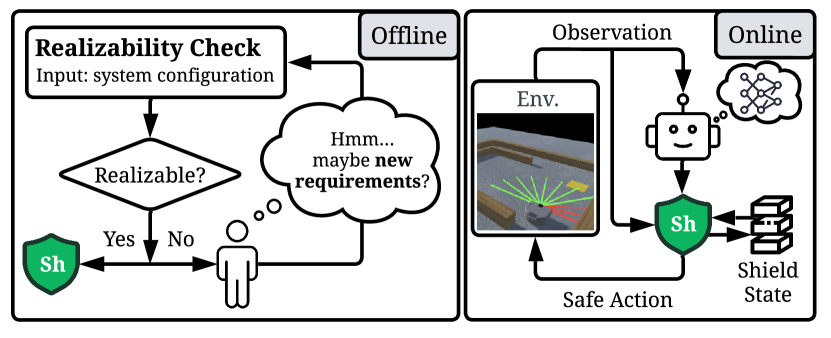
Figure 1: In the offline process, the realizability check verifies whether the system is realizable, taking the system configuration as input, i.e., the dynamics of the environment, the safety requirements, and the input domain. If not realizable, the system needs to be changed. When proved to be realizable (i.e., a Proper Shield), the shield can be safely deployed in the environment for the online process.

Traditional techniques to address safety concerns aim to embed this aspect as part of the learning process; some examples include reward shaping (Tessler, Mankowitz, and Mannor 2018), constrained reinforcement learning (Achiam et al. 2017; Ray, Achiam, and Amodei 2019), and adversarial training (Pinto et al. 2017). While these approaches can significantly improve the general reliability of the policy, they often provide only empirical guarantees, and the benefits are often presented in expectation (Srinivasan et al. 2020; He, Zhao, and Liu 2023). Although these may be sufficient for many problems, they cannot guarantee the safety of a system, which prevents their application in particularly safety-critical contexts.

In contrast, a promising family of approaches provides formal safety guarantees through the adoption of an external component, commonly referred to as a shield (Garcıa and Fernández 2015; Corsi et al. 2024b). In DRL, a shield acts as a protective wrapper over the agent to ensure that its actions remain within safe boundaries, effectively preventing it from making dangerous or undesired decisions. However, most of the shielding techniques presented in the literature face a critical challenge: there are instances where no available action exists that satisfies all safety criteria simultaneously (Alshiekh et al. 2018). In practice, when the shielding mechanism encounters such scenarios, it fails to provide a safe action, leading to unsafe outcomes.

In this paper, we consider this crucial aspect of safety requirement satisfiability for all states. We define a Proper Shield as a shield that is always able to return an action that respects the given specifications for any state of the system (a formal definition is presented as Def. 1).

In the logic community, ensuring this property is equivalent to guaranteeing the realizability property for the shield (a formal definition is provided in section 3). However, it is particularly challenging for a human to provide a shield with safety requirements that it can always satisfy due to the compounding complexity of multiple safety requirements over continuous state and action spaces with many possible scenarios that can occur. Thus to prevent deploying a shield with unrealizable safety requirements, we propose an approach that includes an automatic realizability check as part of an offline procedure performed before deployment (an overview of the overall pipeline is provided in Fig.1). Intuitively, if the shield is not realizable, it means that the system cannot be safe in the required sense, and it is necessary to modify the dynamics of the system or relax the safety specifications. However, there is a scarcity of tools in the literature that support automatic realizability checking. A prominent example is the work of Alshiekh et al. (2018), which proposes to design a shield relying on the concept of Linear Temporal Logic (LTL). Their approach in particular allows the synthesis of the shield as a formal tool to automatically guarantee the realizability of the system. However, this technique comes with a crucial limitation: the synthesizer for the LTL specifications is designed to handle only discrete states and actions. This constraint is overly restrictive for real-world reinforcement learning applications such as robotics where the state and action spaces are often continuous and high dimensional.

This paper primarily builds upon the recent work on Realizability Modulo Theories of Rodríguez and Sánchez (2023). Applying their proposed satisfiability and realizability solver, we introduce a framework that for the first time is able to generate a Proper Shield capable of handling continuous state and action spaces. This significant advance allows us to augment a realizable shield with the benefits that come with using continuous state and action spaces. Firstly, our approach allows us to use optimization techniques to return actions that are not only safe but also closely aligned with the original decisions proposed by the neural network. This ensures that the agent’s behavior remains as optimal and effective as possible while adhering to safety constraints. Secondly, our method allows us to incorporate robot dynamics directly into the safety requirements, allowing for a more accurate model-based representation of the physical world in which the agent’s shield operates.

In addition, we formally prove that with our approach realizability can be verified with a stateful shield. This capability is crucial as it allows us to encode and enforce safety requirements that span multiple steps in the environment. Moreover, we demonstrate the effectiveness of our shielding approach in a mapless navigation domain, with additional experiments in a particle world multi-agent environment. We guarantee the realizability of safety requirements and ensure safety with continuous states and actions without compromising policy performance. To better understand the main contributions of our method and its position in existing literature, Table 1 presents a comparison with alternative techniques, highlighting the strengths of our approach compared to the baselines.

2 Related Work

Safe reinforcement learning aims to develop policies that not only optimize performance but also respect safety constraints, preventing the agent from taking actions that could lead to harmful or undesirable outcomes. In the literature, this safety aspect can be approached from many different perspectives. A first family of approaches attempts to enforce safer behavior as part of the learning process. An example is constrained reinforcement learning, where the MDP is enriched with a cost function to minimize that represents the safety requirements (He, Zhao, and Liu 2023; Achiam et al. 2017; Liu, Ding, and Liu 2020; Ray, Achiam, and Amodei 2019). Other algorithms focus on reward shaping approaches (Tessler, Mankowitz, and Mannor 2018), policy transfer (Simão, Tindemans, and Spaan 2022), behavioral monitors (Corsi et al. 2022; Srinivasan et al. 2020), or on techniques that can guarantee safe exploration and data collection phases (Marvi and Kiumarsi 2021). However, these approaches are not designed to provide formal guarantees about the final policy, especially in the context of deep learning where neural networks are known to be vulnerable to specific input configurations even when trained with state-of-the-art algorithms (Szegedy et al. 2013). Other approaches rely on verification methods to provide guarantees about the behavior of the neural network (Katz et al. 2019; Wang et al. 2021; Katz et al. 2017); however, they suffer from significant scalability problems and are limited in neural network topology (Liu et al. 2021). Moreover, as many recent papers have shown, as the number of requirements grows, it becomes nearly impossible to find models that formally respect the requirements over the entire input space (Corsi et al. 2024a; Amir et al. 2023).

3 Preliminaries

Reinforcement Learning (RL). We model interaction with an environment with a Partially Observable Markov Decision Process (POMDP), defined by a tuple $(X,A,O,P,R,\Omega,\gamma)$, with a state space of $X$, action space $A$, and observation space $O$. $P:X\times A\to\Delta(X)$ represents the state transition function. $R:X\times A\to\mathbb{R}$ is the reward function. $\Omega:X\to\Delta(O)$ represents the observation function, and $\gamma\in[0,1]$ is the discount factor. Our objective is to learn a policy $\pi:O\to\Delta(A)$ that maximizes the expected sum of discounted rewards over time. This is defined as $\mathbb{E}\left[\sum_{t=0}^{T}\gamma^{t}R(x_{t},a_{t})\right]$, where $x_{t}$, $a_{t}$, and $o_{t}$ are the state, action, and observation at time $t$ until the episode horizon $T$.

Reactive Synthesis

LTL.

Linear Temporal Logic (LTL) is a formal system for reasoning about the behavior of discrete-time systems over an infinite timeline. Concretely, it is a modal logic that extends propositional logic with temporal operators that allow the expression of properties about the future evolution of the system. Some key temporal operators in LTL are defined as follows: (1) $\ocircle$ (next): The property holds in the next timstep; (2) $\diamond$ (eventually): The property will eventually hold at some future time; (3) $\square$ (globally): The property holds at all future timsteps and (4) $\mathcal{U}$ (until): A property holds until another property becomes true. Using these operators, LTL formulae can express a wide range of temporal properties such as safety (“something bad never happens”) and liveness (“something good eventually happens”). For instance, while in classic propositional logic we can express $v^{1}\rightarrow v^{2}$, in LTL we can also express $\square(v^{1}\rightarrow\ocircle v^{2})$, which means that at every step, if $v^{1}$ holds, then $v^{2}$ must hold in the next timestep. Recently, Rodríguez and Sánchez (2024b) solved the problem of reactive synthesis for LTL modulo theories (LTLt), an extension of LTL where literals may contain variables of a first-order theory T. They also studied the problem of shield synthesis in LTLt, allowing shields to enforce expressive properties such as $(v^{1}>2)\implies\ocircle(v^{2}>v^{1})$.

Satisfiability.

Given an LTL formula $\varphi$, the satisfiability problem determines if there is any possible execution that satisfies the specified temporal properties; i.e., we say $\varphi$ is satisfiable if there is a possible assignment of the variables in $\varphi$ such that $\varphi$ is satisfied. More formally, given variables $v=\{v^{0},v^{1},...\}$ in $\varphi$, if $\exists v$ s.t. $\varphi(v)$ holds, then $\varphi$ is satisfiable.

Figure 2: The Mapless Navigation environment (Left) and the Particle World environment (Right).

Realizability.

In reactive systems, the system must continuously interact with its environment and adapt its behavior accordingly. Thus, we need a property stronger than satisfiability: realizability, in which the variables of $\varphi$ are split into an uncontrollable player (i.e., the inputs provided by the environment) and a controllable player (i.e., the outputs provided by the system). Then, a formula $\varphi$ is realizable if for all possible valuations of the input variables, the output variables can be assigned so that the $\varphi$ is not violated. More formally, given environment variables $e^{0},e^{1},...$ and system variables $a^{0},a^{1},...$ of $\varphi$, if $(\forall e^{0},e^{1},...\exists a^{0},a^{1},...)^{*}$ s.t. $\varphi(e^{0},e^{1},...,a^{0},a^{1},...)$, then $\varphi$ is realizable. Moreover, if $\varphi$ is realizable, there is some strategy of the system: i.e., a way to assign the variables it controls such that $\varphi$ is never violated. The problem of computing such a strategy in realizable $\varphi$ is called reactive synthesis.

4 Continuous Shields

We now introduce our concept of a Proper Shield which is guaranteed to be realizable, providing safe alternatives to unsafe actions in all states. Working in a POMDP, we instantiate our shield as a stateful component where the shield’s state $h\in H$ is defined as the sequence of the constraints that held in the previous timesteps for an episode. To connect components in RL with the concepts in LTL, we consider the observation $o=\{o^{0},o^{1},...\},o\in O$ and $h\in H$ to be the uncontrollable variables and the action $a=\{a^{0},a^{1},...\},a\in A$ as the controllable variables.

Definition 1 (Proper Shield)

A Proper Shield is a function $\zeta:A\times O\times H\to A$, such that $\forall$ $o\in O$ and $h\in H$, $\varphi(\zeta(a,o,h),o,h)$ holds.

While we focus on the continuous case, this definition holds for both continuous and discrete spaces. In the following sections, we describe how we implement the offline realizability check and the online shielding process for continuous state and action spaces.

Architecture Overview

In this paper we show how to use shield-synthesis, where reactive synthesis computes a shield $\zeta$ from $\varphi$ (in LTL modulo real arithmetic, i.e., continuous domains) and $\zeta$ is combined with an external agent $\pi$ (in our case, an RL-trained agent) to ensure that the composition $\pi\cdot\zeta$ will never violate $\varphi$. In each timestep, given the shield history $h$: (1) $\pi$ receives observation inputs $o$ from the environment and produces action outputs $a$; (2) $\zeta$ checks whether $\varphi(a,o,h)$ holds; and (3) if $\varphi(a,o,h)$ holds, the shield does not intervene, whereas in case of a violation, it overrides $a$ with a correction $\hat{a}=\zeta(a,o,h)$ such that $\varphi(\hat{a},o,h)$ now holds in that step.

This online process translates to providing a valid action (i.e., the assignment of the variables controlled by the system) that satisfies the specified requirements given the current state of the environment. The shield will propagate the continuous constraints through time and will check if the agent’s action satisfies all requirements and otherwise provide an alternative safe action. In LTLt, this is done by performing a query to a constraint satisfaction solver. If the constraint specification is not realizable, the shield may return an unsatisfiable (UNSAT) result, indicating that no safe action is possible given the current state.

In our framework (see Fig. 1(left)) we first check offline whether $\varphi$ is realizable, which ensures that for any possible state of the environment, the shield can always return a safe action. Moreover, since the continuous domain is a metric space, we can measure how far the correction is from the original candidate output. Therefore, we can also optimize the shield’s safe-action correction by returning the safe value closest to the agent’s proposed action.

Non-Markovian Requirements

We now demonstrate how to encode complex non-Markovian requirements in a decidable way and how to enforce them using shields. In computational logic, a problem is considered decidable if there is an algorithm that can determine the truth of any statement in a finite amount of time. However, reactive synthesis for general Linear Temporal Logic modulo theories (LTLt) is not always decidable. For example, synthesis for expressions like $\square(y>\lhd x)$ is undecidable. In this context, the $\lhd$ operator represents a specific value that the variable $x$ has taken in previous timesteps, adding to the complexity of the synthesis problem.

Although semi-decidable methods can be used (Katis et al. 2018; Choi et al. 2022), in safety-critical contexts we are interested in sound and complete processes; thus, we need to specify in the decidable Non-Cross State (NCS) (Geatti et al. 2023) fragment that does not allow the $\lhd$ operator. Although NCS may not look expressive enough for shielding continuous reinforcement learning, we now show that we can effectively encode realistic dynamics of the environment in the predicates of $\varphi$, without the need of such expressive operators. Instead of using the value a variable assumed at timestep $t$, we rely on the boolean output of the LTLt expression at the same timestep.

Example 1

For instance, consider the following non-markovian specification: if the robot is in region $r\in R$, then it cannot visit $r$ again in at least $i$ timesteps. Moreover, let dynamics of positions $(x,y)$ of the robot in step $k$ be precisely characterized by valuations of variables in step $k-1$. We can formally state this in:

$$\square[(x= \lhd\cos(\theta)\cdot\lhd d+x)\wedge(y=\lhd\sin(\theta)\cdot\lhd d+y)]$$

$$\implies\varphi\wedge\square [\bigwedge_{r\in R}[(r_{b}^{x}\leq x\leq r_{u}^{x})\wedge(r_{b}^{y}\leq y\leq r_{u}^{y})]$$

$$\implies \square_{[1,i]}\neg[(r_{b}^{x}\leq x\leq r_{u}^{x})\wedge(r_{b}^{y}\leq y\leq r_{u}^{y})]],$$

where $\theta$ and $d$ correspond to the angle and distance decided by the system (based on environment observations that are modelled in the safety property $\varphi$). In natural language, the first line of the specification describes the dynamics of $(x,y)$, whereas the second and third line describe that if $(x,y)\in r$ then $(x,y)\notin r$ throughout $i$ timesteps. Note that this specification is syntactically encoded in a fragment of LTLt that is not decidable. However, we can rewrite it in the NCS fragment of LTLt with the formula $A\rightarrow G$, where $A$ are the following assumptions contraining the dynamics of the environment:

$$\square[\bigwedge_{r\in R}\neg[(r^{x_{b}}\leq\cos(\theta)\cdot d+x\leq r^{x_{u}})$$

$$\wedge(r^{y_{b}}\leq\sin(\theta)\cdot d+y\leq r^{y_{u}})]$$

$$\rightarrow\ocircle\neg[(r^{x_{b}}\leq x\leq r^{x_{u}})\wedge(r^{y_{b}}\leq y\leq r^{y_{u}})]],$$

which means that there is no situation in which $\theta$ and $d$ are in $r$ in timestep $k$ and $(x,y)$ of timestep $k+1$ is not in $i$). Moreover, $G$ are the following guarantees that encode what the system should enforce:

$$\square[\bigwedge_{r\in R}[[(r^{x_{b}}\leq\cos(\theta)\cdot d+x\leq r^{x_{u}})\wedge$$

$$(r^{y_{b}}\leq\sin(\theta)\cdot d+y\leq r^{y_{u}})]$$

$$\rightarrow\square_{[1,i]}\neg[(r^{x_{b}}\leq\cos(\theta)\cdot d+x\leq r^{x_{u}})$$

$$\wedge(r^{y_{b}}\leq\sin(\theta)\cdot d+y\leq r^{y_{u}})]]],$$

which means that, if $\theta$ and $d$ are in $r$ in timestep $k$, then throught $i$ timesteps, $\theta$ and $d$ must be chosen so that they are not in $r$).

In general, if $\varphi$ is an LTLt formula where all the appearances of the $\lhd$ operator are isolated and are used in assignments, then $\varphi$ can be rewritten in NCS, which means that realizability for $\varphi$ is decidable for a precise formalization).

5 Case Study: Mapless Navigation

In this section, we present the main case study of this work, describing the environment we use, the safety challenges it presents, and the safety specifications we aim to guarantee with a proper shield over our RL agent.

Navigation with Reinforcement Learning

The goal of our agent is to navigate through an unknown environment to reach a target position while avoiding collisions with obstacles. This problem is particularly challenging from a safety perspective due to the partial observability of the environment. In every episode, we randomly set the position of the agent’s starting point, target destination, and the placement of obstacles. The agent can only perceive its immediate environment via a lidar scan, providing scalar distances to nearby obstacles in a finite set of directions. In addition to lidar, observations include the agent’s current position, orientation, and target location. We define the environment’s action space as the linear and angular velocity of the robot (we provide additional details about the training environment in Appendix B). The reward function for this environment incentivizes the agent to reach its target position by avoiding the obstacles and additionally provides a penalty to encourage the robot to reach the target with the minimum possible number of steps; more formally:

$$R(s,a)=\begin{cases}1&\text{agent reaches the target}\\ -1&\text{agent collides with an obstacle}\\ -0.01&\text{at each timestep otherwise}\end{cases}$$

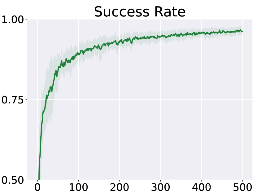
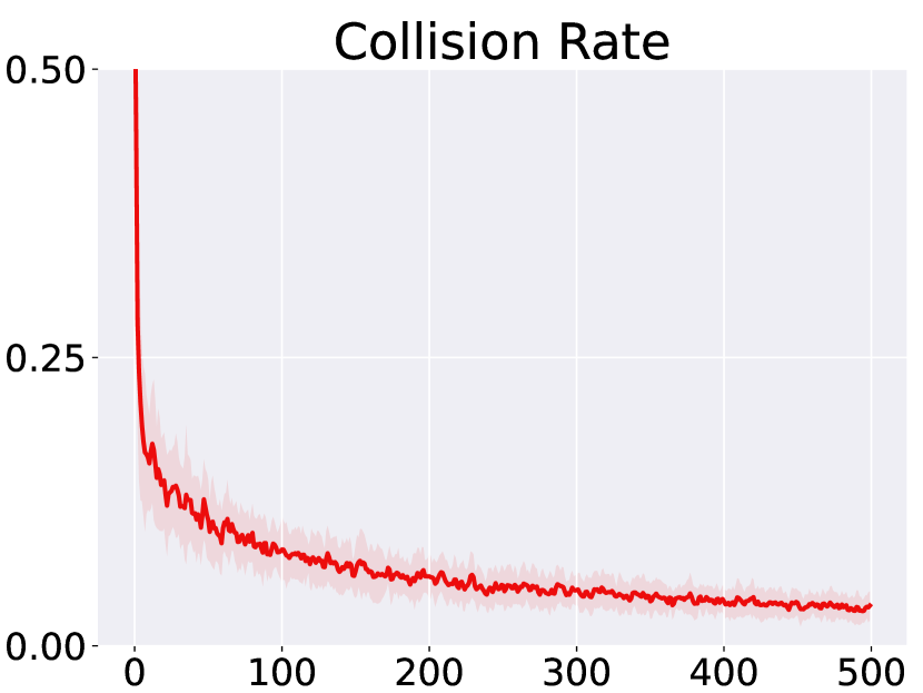
Figure 3: Average success rate and collision rate obtained during the DRL training process for 500 episodes (x-axis) without any shield applied (averaged over $5$ different random seeds). We reach an imperfect final collision rate of 1.2%, highlighting the need for a shield to prevent dangerous failures.

To train our agent, we employ Proximal Policy Optimization (PPO) (Schulman et al. 2017), which has been shown to be efficient on similar navigation tasks (Amir et al. 2023). For evaluation, we analyze the success and collision rates of trajectories executed by the agent. Fig.3 illustrates the PPO training process over time. Without any shielding, we see the agent achieve a success rate of 98.1% along with a complementarily low collision rate of 1.2%. However, the collision rate does not reach a constant value of zero, highlighting the persistent risk of unsafe behavior during deployment. This observation underscores the critical need for our proposed shielding approach, which aims to enforce robust safety guarantees and mitigate the remaining risks inherent in complex and dynamic environments.

Continuous Shield for Safe Navigation

In this section, we delineate the safety requirements we aim to enforce and how we specify them using LTLt to ensure robust and reliable performance. We consider two key aspects: safety (i.e. avoiding collisions) and liveliness (i.e. avoiding repeated action sequences that can lead to a loop).

Requirements for Collision Avoidance

In navigation tasks, ensuring collision avoidance is crucial under all circumstances. To achieve this, we encode specifications by leveraging the dynamics of the robot, made feasible by our framework’s ability to handle continuous spaces. Given an action $a=[a^{0},a^{1}]$, the robot first rotates by $a^{1}$ and then translates by $a^{0}$, where $a^{0}\in[-L^{0},L^{0}]$ and $a^{1}\in[-L^{1},L^{1}]$ and $L^{N}$ is a step size. Positive $a^{0}$ indicates forward motion and positive $a^{1}$ means a right turn. As the next pose of the robot is predictable through the dynamics, we can design requirements that strictly avoid collisions in the next timestep. Since robot rotation and translation are performed sequentially in the environment dynamics, requirements for each can be designed separately. Specifically, the red area in Fig. 4 (left) shows the robot’s trajectory when it makes a maximum right turn of $L^{1}$. To conservatively prevent collisions from right turns, we prohibit turning right if any lidar value $l^{i}$ is below a certain threshold $T^{i}$. These thresholds are precomputed based on the robot’s dynamics and maximum step size $L^{1}$ and they vary for each lidar (highlighted in blue). Formally, the specification for a right turn is: $\exists i$ s.t. $\,(l^{i}\leq T^{i})\rightarrow a^{1}\leq 0$. The same principle applies to left turns.

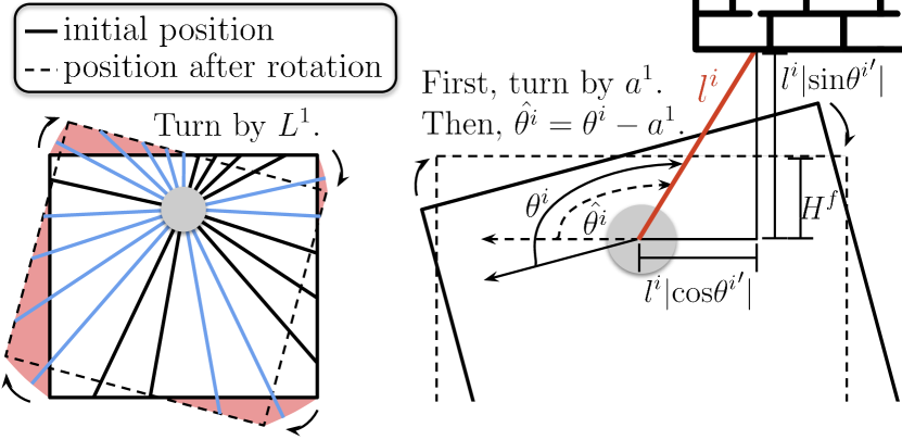
Figure 4: Description of collision avoidance requirements that include the dynamic of the robot as part of the formula.

For translation, we limit the maximum distance that we can translate based on the minimum distance of potential obstacles that any lidars sense in the direction of travel. Consider the $i^{th}$ lidar with value $l^{i}$ at an angular position $\theta^{i}$ relative to the robot’s horizontal line, measured clockwise from the left. Note that $\theta^{i}$ is known by construction as part of the system. After the robot rotates by $a^{1}$, the angular position w.r.t. the new horizontal line becomes $\hat{\theta^{i}}=\theta^{i}-a^{1}$. If this lidar reveals that the obstacle is in the path of forward translation, the translation $a^{0}$ cannot exceed the distance to the obstacle; otherwise, a collision will occur. Formally, the requirement for forward translation w.r.t. the $i^{th}$ lidar is: $l^{i}|\textrm{cos}{\theta^{i}}^{\prime}|\leq\frac{W}{2}\rightarrow a^{0}+H^{f}<l^{i}|\textrm{sin}{\theta^{i}}^{\prime}|$, where $W$ is the robot’s width and $H^{f}$ is the lidar’s forward offset. For forward translation, this requirement must hold for all lidars in front of the robot. Similar requirements apply for backward translation, with different signs, offsets, and considering lidars at the back.

		$G^{A}$
		3	5	30
$L^{Q}$	1	31	0	0
	13	288	6	0
	100	336	30	0

Table 2: Number of episodes where the shield returns unsat out of 500 test episodes with different $L^{Q}$ and $G^{A}$. Configurations verified as realizable are highlighted in green, otherwise in red. realizability checking can reveal the existence of situations in which specifications are unsatisfiable that empirical evaluation may fail to indicate.

Requirements for Liveness

While safety remains paramount in autonomous systems, ensuring collision avoidance, etc. alone can lead to overly conservative behavior, often characterized by repetitive or looping actions. The agent then can be particularly inefficient, wasting time and energy. To address this issue, we introduce a set of important liveness requirements. These prohibit repeating the same action in a state for a certain time window. This encourages the agent to explore new actions, potentially helping it escape from being stuck. We encode these requirements using a queue constructed from the shield state of length $L^{Q}$. Each queue element consists of the robot’s pose (x/y position and rotation) and actions, represented as $(x,y,r,a^{0},a^{1})$. To effectively check for repeated tuples of continuous values, we quantize the pose and action space into grids of $G^{P}$ and $G^{A}$ cells, respectively. In this way, the shield does not allow an action $(a^{0},a^{1})$ in a state $(x,y,r)$ if any of the previous tuples in the queue falls into the same cell. As the liveness requirements take stateful memory as an additional input, they are non-Markovian requirements and however, don’t affect the realizability check in our approach.

Realizability and Shielding Implementation

We specify the above requirements in LTLt and provide them to our offline realizability check process to guarantee that these safety and liveness requirements are always satisfiable. Our realizability check process follows the implementation established in (Rodríguez and Sánchez 2023, 2024a, 2024b; Rodríguez, Gorostiaga, and Sánchez 2024). After realizability for our requirements is guaranteed, at test-time, we deploy our agent with an online shield to provide safe alternative actions when the agent suggests an action that violates our constraints. We present our LTLt requirements and the overall algorithm for deploying the online shield in the appendices.

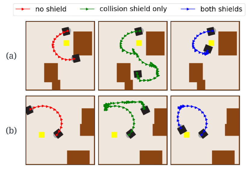
Figure 5: An unshielded agent collides with obstacles and avoids them when a collision shield is applied. By introducing liveness requirements, the agent also avoids oscillations and reaches its target destination.

No Shield Safety Shield Safety & Liveness Shield Optimizer Success Collision Success Collision Success Collision Success Collision Expert A 0.87 $\pm$ 0.05 0.03 $\pm$ 0.03 0.87 $\pm$ 0.04 0.00 $\pm$ 0.00 0.90 $\pm$ 0.02 0.00 $\pm$ 0.00 0.92 $\pm$ 0.02 0.00 $\pm$ 0.00 Expert B 0.88 $\pm$ 0.03 0.03 $\pm$ 0.02 0.87 $\pm$ 0.03 0.00 $\pm$ 0.00 0.90 $\pm$ 0.02 0.00 $\pm$ 0.00 0.90 $\pm$ 0.02 0.00 $\pm$ 0.00 Moderate A 0.77 $\pm$ 0.04 0.01 $\pm$ 0.01 0.76 $\pm$ 0.04 0.00 $\pm$ 0.00 0.79 $\pm$ 0.04 0.00 $\pm$ 0.00 0.80 $\pm$ 0.05 0.00 $\pm$ 0.00 Moderate B 0.85 $\pm$ 0.02 0.04 $\pm$ 0.02 0.85 $\pm$ 0.02 0.00 $\pm$ 0.00 0.87 $\pm$ 0.02 0.00 $\pm$ 0.00 0.87 $\pm$ 0.02 0.00 $\pm$ 0.00 Unsafe 0.22 $\pm$ 0.03 0.78 $\pm$ 0.03 0.40 $\pm$ 0.05 0.00 $\pm$ 0.00 0.47 $\pm$ 0.02 0.01* $\pm$ 0.01 0.69 $\pm$ 0.03 0.01* $\pm$ 0.00

Table 3: Comparison of success rate and collision rate with different settings of the shield on the mapless navigation environment. Mean scores over 5 seeds (100 runs per seed) with standard deviations are presented. *These collisions arose due to the partial observability in the environment and can be prevented by increasing the number of 1D lidar sensors.

6 Experimental Results

In this section, we present the results of our experiments, demonstrating the effectiveness of our proposed realizability check and shielding approach.

Mapless Navigation Experiments

Realizability Check

A crucial aspect of our shield is that it guarantees a safe action in any state through a realizability check. Ensuring realizability by hand is challenging with complex requirements like ours, and statistics-driven safety checks are also unreliable.

In Tab. 2 we evaluate a shielded agent for 500 episodes with multiple different queue lengths ($L^{Q}$) and action grid sizes ($G^{A}$) without performing a realizability check beforehand. We then tally the number of times we encountered a unsat output from the shield due to no safe action being available. Finally, we verify the realizability of each shield specification and highlight the realizable configuration in green. We see that performing a realizability check can warn us about potentially unsatisfiable and thus unsafe specifications even when empirical evaluations do not indicate a problem. For instance, no unsat situations occurred for our shield with evaluating $(L^{Q},G^{A})=(100,30)$, however, our realizability check reveals that there still are potential situations where $(100,30)$ is not satisfiable. For subsequent experiments, we use one of the verified realizable configurations, $(L^{Q},G^{A})=(30,13)$.

Online Shielding

In Table 3, we report the analysis of 5 different RL agents with different capabilities. Expert A and Expert B are fully trained PPO models. Moderate A and Moderate B are checkpoints collected during an intermediate phase of learning and are more prone to making mistakes and failing the task. Finally, Unsafe is Expert A deployed without access to lidar data, simulating a dangerous agent oriented toward unsafe behavior and collisions. We believe that the addition of unsafe models is particularly valuable for our analysis to show that the shield can be effective with any model and guarantee safety independently of the input policy.

The first column shows the success rate and collision rate when each policy is executed without any external shielding component. Although the success rates for the well-trained agents could be considered satisfactory, all agents made some collisions with an obstacle. The second column shows each policy’s performance with the collision avoidance shield added, clearly demonstrating the effectiveness of our shield, which reduces the number of collisions to zero. However, the shield alone leads to overly conservative behavior, resulting in the unsafe trajectories being converted into timeouts with oscillating behavior rather than successful episodes. Crucially, the third column shows the complete version of our shield (i.e., with both collision avoidance and liveness requirements), showing that the satisfaction of both properties allows the agent to recover from the conservative behavior and increase the success rate while ensuring the safety of the policy. Finally, the last column shows a small additional impact of optimizing the shield’s choice of safe action. Since we operate in a continuous space, our shield can employ an optimizer to return a safe action that minimizes distance to the original policy output. In this navigation domain, we minimize $|{\hat{a}^{1}}-a^{1}|$ where $a^{1}$ is the agent’s original angular velocity and ${\hat{a}^{1}}$ is the angular velocity of the shielded action. Fig. 5 illustrates a policy’s behavior both with and without a shield employed for collisions and liveness.

Particle World Experiments

To further demonstrate the generalizability and robustness of our shielding approach, we also experiment in a multi-agent Particle World environment (Mordatch and Abbeel 2017). Four agents are tasked with reaching target positions on the opposite side of the map while maintaining a safe distance from one another. Fig. 2 (Right) shows a screenshot of this environment where agents are represented as dots. The primary safety requirement in this environment is to ensure that the agents always keep a specified minimum distance between each other, illustrated as circles around the agents. The results, summarized in Table 4, demonstrate that our safety shield can be seamlessly applied to this new environment with a continuous state and action space. Notably, our shielding technique in Particle World successfully eliminates all violations of the safety requirements, effectively preventing any unsafe actions. This highlights the versatility and effectiveness of our shielding approach, showcasing its potential for broader applications across various continuous-space environments.

No Shield Safety Shield Success Collision Success Collision Model A 0.56 $\pm$ 0.06 0.46 $\pm$ 0.05 0.93 $\pm$ 0.02 0.00 $\pm$ 0.00 Model B 0.53 $\pm$ 0.05 0.49 $\pm$ 0.07 0.95 $\pm$ 0.01 0.00 $\pm$ 0.00 Model C 0.64 $\pm$ 0.03 0.36 $\pm$ 0.03 0.96 $\pm$ 0.00 0.00 $\pm$ 0.00 Model D 0.66 $\pm$ 0.02 0.35 $\pm$ 0.02 0.97 $\pm$ 0.01 0.00 $\pm$ 0.00

Table 4: Results on the Particle World environment. The No Shield agent is completely blind to the safety requirements and is therefore not trained to avoid collisions. Given the full observability of this environment, it is possible to exploit the dynamics of the system to cover all possible sources of collisions, reducing this number to zero.

7 Conclusion

In this paper, we introduce the concept of Proper Shield and develop a novel approach to creating a shield that can handle continuous action spaces while ensuring realizability. Our results demonstrate that this shielding technique effectively guarantees the safety of our reinforcement learning agent in a navigation problem. A significant achievement of our work is a theoretical and empirical integration of liveness requirements into the shielding process. This integration helps mitigate overly conservative behaviors, enabling the agent to recover from loops and repeated actions caused by strict safety specifications, maintaining efficient progress toward its goals. As a limitation, while our definition of a proper shield ensures a response for every state, an exhaustive realizability check may be overly cautious. Some states may not be reachable by a shielded agent and thus not require satisfiability, a factor not considered in our analysis. We plan to investigate this aspect and relax the constraints as a direction for future research.

A major bottleneck in deploying a safe agent for the navigation domain was generating reasonable safety requirements that were also realizable. Looking ahead, we plan to investigate ways to simplify the procedure for generating realizable safety requirements and allow safe RL agents to be more easily deployed across a wide variety of new domains.

Appendix A Algorithm and Implementation Details

In this section, we describe how the shield is deployed in the online process. Alg. 1 provides a pseudocode of the shielded reinforcement learning loop equipped with the optimizer. We define general rules for requirements $Reqs$ which is instantiated as $reqs$ for given state $s$ and queue $Q$ for each time step. Note that these $Reqs$ are verified realizable in the offline process. And, we have two shield components, $Sol$ and $Opt$, which return an action that respects the $reqs$. $Opt$ is more advanced as it can bake in additional criteria to optimize, which is possible as our shield is capable of handling continuous spaces. For example, one effective criterion can be minimizing the distance to the original action $a$. By doing so, the returned safe action will be closely aligned with the original decision. On the other hand, $Sol$ will return any safe action that satisfies the specifications which might not be optimal in terms of achieving a goal. For each time step, we first select an action from the policy $\pi$. If this action satisfies the requirements $reqs$, we perform that action as it is verified safe. Otherwise, we run the optimizer with a time limit $T_{Opt}$. If the optimizer fails to compute an action in time, we fall back to the action from $Sol$.

Algorithm 1 Shielded Reinforcement Learning Loop

0:  Trained RL agent $\pi$, environment $env$, episode length $T$, requirements $Reqs$, solver $Sol$, optimizer $Opt$ with timeout $T_{Opt}$, queue length $L_{Q}$

1:  Reset the environment: $s\leftarrow env.reset()$

2:  Initialize total reward $R\leftarrow 0$ and queue $Q\leftarrow\emptyset$ of length $L_{Q}$

3:  for each step $t=1,2,\ldots,T$ and not $terminated$ do

4:     Select action $a\leftarrow\pi(s)$

5:     $reqs\leftarrow Reqs(s,Q)$

6:     if $a$ satisfies $reqs$ then

7:        $a_{safe}\leftarrow a$

8:     else

9:        $a_{opt}\leftarrow Opt(reqs,T_{Opt})$

10:        if $a_{opt}$ is not $None$ then

11:           $a_{safe}\leftarrow a_{opt}$

12:        else

13:           $a_{safe}\leftarrow Sol(reqs)$

14:        end if

15:     end if

16:     $(s,r,terminated)\leftarrow env.step(a_{safe})$

17:     Update total reward: $R\leftarrow R+r$

18:     $Q.\text{enqueue}(s_{x},s_{y},s_{o},a_{safe}[0],a_{safe}[1])$ {Automatically pops oldest element if length exceeds $L_{Q}$}

19:  end for

20:  return  Total reward $R$

Appendix B Training Details

We ran our experiments on a distributed cluster with 255 CPUs and 1T RAM. Each individual training loop was performed on 2 CPUs and 6GB of RAM, for a total wall time of approximately 15 hours. We perform the training with a customized implementation of the Proximal Policy Optimization algorithm (Schulman et al. 2017) from the CleanRL repository. Following is the complete list of hyperparameters and a detailed explanation of the state and action spaces.

General Parameters

• training episodes: 500

• number of hidden layers: 2

• size of hidden layers: 32

• activation function: ReLU

• parallel environments: 1

• gamma ($\gamma$): 0.99

• learning rate: $0.0015$

PPO Parameters

For the advantage estimation and the critic update, we rely on the Generalized Advantage Estimation (GAE) strategy. The update rule follows the guidelines of the OpenAI’s Spinning Up documentation. Following is a complete list of the hyperparameters for our training:

• memory limit: None

• update frequency: 4096 steps

• trajectory reduction strategy: sum

• actor epochs: 30

• actor batch numbers: 32

• critic epochs: 30

• critic batch numbers: 32

• critic network size: 2x256

• PPO clip: 0.2

• GAE lambda: 0.8

• target kl-divergence: 0.02

• max gradient normal: 0.5

• entropy coefficent: 0.001

• learning rate annealing: yes

Random Seeds for Reproducibility:

To obtain the best performing models for our analysis, we applied the following random seeds [$2$, $12$, $18$, $9$, $5$, $1$, $11$] to the following Python modules Random, NumPy, and PyTorch.

State and Action Spaces:

The Mapless Navigation environment follows the structure proposed in Corsi et al. (2024b), more in details:

• The state space constitutes of $30$ continuous values: the first $23$ variables represent lidar sensor readings, that indicate the distance from an obstacle in a given direction (from left to right, with a step of $\approx 15^{\circ}$). The following $4$ variables represent the (x, y) position of respectively agent and target position. An additional variable indicates the orientation of the agent (i.e., compass). The last $3$ observations are the relative position of the target with respect to the agent in polar coordinates (i.e., heading and distance). All these values are normalized in the interval $[0,1]$ and can take on any continuous values within this interval.

• The action space consists of $2$ continuous variables: the first one indicates the linear velocity (i.e., the speed of the robot), and the second one provides the angular velocity (i.e., a single value indicating the rotation). These two actions can be executed simultaneously, providing the agent with richer movement options.

References

- Achiam et al. (2017) Achiam, J.; Held, D.; Tamar, A.; and Abbeel, P. 2017. Constrained policy optimization. In International conference on machine learning.
- Alshiekh et al. (2018) Alshiekh, M.; Bloem, R.; Ehlers, R.; Könighofer, B.; Niekum, S.; and Topcu, U. 2018. Safe reinforcement learning via shielding. In Proceedings of the AAAI conference on artificial intelligence.
- Amir et al. (2023) Amir, G.; Corsi, D.; Yerushalmi, R.; Marzari, L.; Harel, D.; Farinelli, A.; and Katz, G. 2023. Verifying learning-based robotic navigation systems. In International Conference on Tools and Algorithms for the Construction and Analysis of Systems. Springer.
- Aractingi et al. (2023) Aractingi, M.; Léziart, P.-A.; Flayols, T.; Perez, J.; Silander, T.; and Souères, P. 2023. Controlling the Solo12 quadruped robot with deep reinforcement learning. scientific Reports.
- Berner et al. (2019) Berner, C.; Brockman, G.; Chan, B.; Cheung, V.; Debiak, P.; Dennison, C.; Farhi, D.; Fischer, Q.; Hashme, S.; Hesse, C.; et al. 2019. Dota 2 with large scale deep reinforcement learning. arXiv preprint arXiv:1912.06680.
- Choi et al. (2022) Choi, W.; Finkbeiner, B.; Piskac, R.; and Santolucito, M. 2022. Can reactive synthesis and syntax-guided synthesis be friends? In Jhala, R.; and Dillig, I., eds., 43rd ACM SIGPLAN Int’l Conf. on Programming Language Design and Implementation (PLDI 2022), 229–243. ACM.
- Corsi et al. (2024a) Corsi, D.; Amir, G.; Katz, G.; and Farinelli, A. 2024a. Analyzing Adversarial Inputs in Deep Reinforcement Learning. arXiv preprint arXiv:2402.05284.
- Corsi et al. (2024b) Corsi, D.; Amir, G.; Rodriguez, A.; Sanchez, C.; Katz, G.; and Fox, R. 2024b. Verification-Guided Shielding for Deep Reinforcement Learning. The 1st Reinforcement Learning Conference (RLC).
- Corsi, Marchesini, and Farinelli (2021) Corsi, D.; Marchesini, E.; and Farinelli, A. 2021. Formal verification of neural networks for safety-critical tasks in deep reinforcement learning. In Uncertainty in Artificial Intelligence.
- Corsi et al. (2022) Corsi, D.; Yerushalmi, R.; Amir, G.; Farinelli, A.; Harel, D.; and Katz, G. 2022. Constrained reinforcement learning for robotics via scenario-based programming. arXiv preprint arXiv:2206.09603.
- Garcıa and Fernández (2015) Garcıa, J.; and Fernández, F. 2015. A comprehensive survey on safe reinforcement learning. Journal of Machine Learning Research.
- Geatti et al. (2023) Geatti, L.; Gianola, A.; Gigante, N.; and Winkler, S. 2023. Decidable Fragments of LTLf Modulo Theories (Extended Version). CoRR, abs/2307.16840.
- He, Zhao, and Liu (2023) He, T.; Zhao, W.; and Liu, C. 2023. Autocost: Evolving intrinsic cost for zero-violation reinforcement learning. In Proceedings of the AAAI Conference on Artificial Intelligence.
- Katis et al. (2018) Katis, A.; Fedyukovich, G.; Guo, H.; Gacek, A.; Backes, J.; Gurfinkel, A.; and Whalen, M. W. 2018. Validity-Guided Synthesis of Reactive Systems from Assume-Guarantee Contracts. In Proc. of the 24th International Conference on Tools and Algorithms for the Construction and Analysis of Systems, (TACAS 2018), volume 10806 of LNCS, 176–193. Springer.
- Katz et al. (2017) Katz, G.; Barrett, C.; Dill, D. L.; Julian, K.; and Kochenderfer, M. J. 2017. Reluplex: An efficient SMT solver for verifying deep neural networks. In Computer Aided Verification 2017. Springer.
- Katz et al. (2019) Katz, G.; Huang, D. A.; Ibeling, D.; Julian, K.; Lazarus, C.; Lim, R.; Shah, P.; Thakoor, S.; Wu, H.; Zeljić, A.; et al. 2019. The marabou framework for verification and analysis of deep neural networks. In Computer Aided Verification 2019.
- Lee (1982) Lee, E. T. 1982. An efficient algorithm for finding kleene closure of regular expression matrices. Int. J. Parallel Program., 11(6): 409–415.
- Liu et al. (2021) Liu, C.; Arnon, T.; Lazarus, C.; Strong, C.; Barrett, C.; Kochenderfer, M. J.; et al. 2021. Algorithms for verifying deep neural networks. Foundations and Trends® in Optimization.
- Liu, Ding, and Liu (2020) Liu, Y.; Ding, J.; and Liu, X. 2020. Ipo: Interior-point policy optimization under constraints. In Proceedings of the AAAI conference on artificial intelligence.
- Marvi and Kiumarsi (2021) Marvi, Z.; and Kiumarsi, B. 2021. Safe reinforcement learning: A control barrier function optimization approach. International Journal of Robust and Nonlinear Control.
- Mordatch and Abbeel (2017) Mordatch, I.; and Abbeel, P. 2017. Emergence of Grounded Compositional Language in Multi-Agent Populations. arXiv preprint arXiv:1703.04908.
- Pinto et al. (2017) Pinto, L.; Davidson, J.; Sukthankar, R.; and Gupta, A. 2017. Robust adversarial reinforcement learning. In International conference on machine learning.
- Pore et al. (2021) Pore, A.; Corsi, D.; Marchesini, E.; Dall’Alba, D.; Casals, A.; Farinelli, A.; and Fiorini, P. 2021. Safe reinforcement learning using formal verification for tissue retraction in autonomous robotic-assisted surgery. In 2021 IEEE/RSJ International Conference on Intelligent Robots and Systems (IROS). IEEE.
- Ray, Achiam, and Amodei (2019) Ray, A.; Achiam, J.; and Amodei, D. 2019. Benchmarking safe exploration in deep reinforcement learning. arXiv preprint arXiv:1910.01708.
- Rodríguez and Sánchez (2023) Rodríguez, A.; and Sánchez, C. 2023. Boolean abstractions for realizability modulo theories. In International Conference on Computer Aided Verification, 305–328. Springer.
- Rodríguez, Gorostiaga, and Sánchez (2024) Rodríguez, A.; Gorostiaga, F.; and Sánchez, C. 2024. Predictable and Performant Reactive Synthesis Modulo Theories via Functional Synthesis. In Proc. of the 22nd International Symposium on Automated Technology for Verification and Analysis (ATVA 2024).
- Rodríguez and Sánchez (2024a) Rodríguez, A.; and Sánchez, C. 2024a. Adaptive Reactive Synthesis for LTL and LTLf Modulo Theories. In Proc. of the 38th AAAI Conf. on Artificial Intelligence (AAAI 2024).
- Rodríguez and Sánchez (2024b) Rodríguez, A.; and Sánchez, C. 2024b. Realizability modulo theories. Journal of Logical and Algebraic Methods in Programming.
- Schulman et al. (2017) Schulman, J.; Wolski, F.; Dhariwal, P.; Radford, A.; and Klimov, O. 2017. Proximal policy optimization algorithms. arXiv preprint arXiv:1707.06347.
- Silver et al. (2016) Silver, D.; Huang, A.; Maddison, C. J.; Guez, A.; Sifre, L.; Van Den Driessche, G.; Schrittwieser, J.; Antonoglou, I.; Panneershelvam, V.; Lanctot, M.; et al. 2016. Mastering the game of Go with deep neural networks and tree search. Nature.
- Simão, Tindemans, and Spaan (2022) Simão, T.; Tindemans, S.; and Spaan, M. 2022. Training and transferring safe policies in reinforcement learning. In Sl: Adaptive and Learning Agents.
- Srinivasan et al. (2020) Srinivasan, K.; Eysenbach, B.; Ha, S.; Tan, J.; and Finn, C. 2020. Learning to be safe: Deep rl with a safety critic. arXiv preprint arXiv:2010.14603.
- Szegedy et al. (2013) Szegedy, C.; Zaremba, W.; Sutskever, I.; Bruna, J.; Erhan, D.; Goodfellow, I.; and Fergus, R. 2013. Intriguing properties of neural networks. arXiv preprint arXiv:1312.6199.
- Tai, Paolo, and Liu (2017) Tai, L.; Paolo, G.; and Liu, M. 2017. Virtual-to-real deep reinforcement learning: Continuous control of mobile robots for mapless navigation. In 2017 IEEE/RSJ international conference on intelligent robots and systems (IROS).
- Tessler, Mankowitz, and Mannor (2018) Tessler, C.; Mankowitz, D. J.; and Mannor, S. 2018. Reward Constrained Policy Optimization. In International Conference on Learning Representations.
- Wang et al. (2021) Wang, S.; Zhang, H.; Xu, K.; Lin, X.; Jana, S.; Hsieh, C.-J.; and Kolter, J. Z. 2021. Beta-crown: Efficient bound propagation with per-neuron split constraints for neural network robustness verification. Advances in Neural Information Processing Systems.