Diffusive interactions between photons and electrons:
an application to cosmology

Abstract

The gradient force is the conservative component of many types of forces exerted by light on particles. When it is derived from a potential, there is no heat transferred to the particle interacting with the light field. However, most theoretical descriptions of the gradient force use simplified configurations of the light field and particle interactions which overlook small amounts of heating. It is known that quantum fluctuations contribute to a very small but measurable momentum diffusion of atoms and a corresponding increase in their temperature. This paper examines the contribution to momentum diffusion from a gradient force described as a quantum interaction between electron wave packets and a classical electromagnetic field. Stimulated transfers of photons between interfering light beams produce a small amount of heating that is difficult to detect in laboratory experiments. However the solar corona, with its thermal electrons irradiated by an intense electromagnetic field, provides ideal conditions for such a measurement. Heating from stimulated transfers is calculated to contribute a large fraction of the observed coronal heating. Furthermore, the energy removed from the light field produces a wavelength shift of its spectrum as it travels through free electrons. Theory predicts a stimulated transfer redshift comparable to the redshift of distant objects observed in astronomy.

1 Introduction

The gradient force manifests itself as a conservative force derived from the gradient of light intensity $\boldsymbol{F}=\boldsymbol{\nabla}I$. A particle interacting with the field of a standing wave will periodically exchange energy and momentum with the intensity pattern generated by interfering light beams. This gives rise to a force without heat transfer from the radiation to the particle. Practical applications such as optical trapping and optical tweezers use the conservative property of the force to manipulate atoms without the temperature increase associated with large optical fields.

At the quantum level, gradient forces are produced by an exchange of momentum between photons and a particle. For the force to exist, the radiation field must have more than one momentum component[1], that is, two beams of light must interact simultaneously with a particle. In a standing wave such as the one depicted in Fig. 1, photons are removed from one plane wave ${\boldsymbol{k}}$ and stimulated into the counter propagating wave ${\boldsymbol{k}}^{\prime}=-{\boldsymbol{k}}$, where ${\boldsymbol{k}}$ is the angular wave vector of the wave. This stimulated transfer changes the momentum of the field by $-2\hbar{\boldsymbol{k}}$ which is taken by the particle as a momentum kick $\Delta{\boldsymbol{p}}=+2\hbar{\boldsymbol{k}}$. The force on the particle is then $\boldsymbol{F}={\mathrm{d}}{\boldsymbol{p}}/{\mathrm{d}}t=\Gamma\Delta{\boldsymbol{p}}$, where $\Gamma$ is the rate of stimulated transfers.

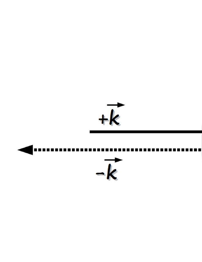
Figure 1: A particle with an initial momentum ${\boldsymbol{p}}=-\hbar{\boldsymbol{k}}$ interacts with a standing wave. One photon is absorbed from beam $+{\boldsymbol{k}}$ and is stimulated into beam $-{\boldsymbol{k}}$, resulting in a momentum $+2\hbar{\boldsymbol{k}}$ being transferred to the particle.

Because of the quantum nature of the gradient force, each momentum kick from a stimulated transfer increases the width of the momentum distribution of the particles.[2, 3] These quantum fluctuations produce momentum diffusion which indicates an increasing temperature of the particles as well as energy being taken away from the radiation field. In general however, quantum fluctuations of the gradient force are very small compared to the force itself. Because most experiments use configurations such as standing waves, far detuned excitation, narrow bandwidth lasers, or collimated particles and fields (plane waves) that minimize quantum fluctuations, contributions to momentum diffusion are neglected in most theoretical calculations of the gradient force.

In this paper I give the broad lines of a calculation of the momentum diffusion resulting from the gradient force on electrons that includes the small contributions from quantum fluctuations. The calculation uses these elements:

• a statistical mixture of travelling waves instead of standing waves,

• a light field with multiple components instead of pure quantum states,

• an electron wave packet instead of a plane wave,

• recoil shifts and Doppler shifts,

• the density matrix formalism for a large ensemble of particles, and

• a second order expansion of the Schrödinger equation.

With this more complex model of stimulated transfers, a number of effects appear as new properties of the gradient force. Two of these are examined in details in this paper: the energy transferred to the electron in the form of heat, and the energy lost by light resulting in a spectral shift toward longer wavelengths.

If a frame of reference contains at least two light beams that can interact with the electron, each stimulated transfer gives a momentum kick to the electron initially at rest in that reference frame. Electrons gain momentum which translates as momentum diffusion and an increase of their temperature. While the temperature increase would be difficult to detect in the laboratory, we will see that the effect is large enough to be observed in the solar corona.

The second effect is the energy lost by the radiation field as it is transferred to the electrons. Each stimulated transfer produces a recoil of the electron which Doppler shifts the stimulated photon to a lower energy. Because every photon transfer is done via stimulated emission, the direction of the beams is preserved while its photons are being replaced by photons with a slightly lower energy. The result is shift toward longer wavelengths of the entire spectrum that preserves its spectral features and directionality. While this frequency shift is difficult to detect in the laboratory, the effect is significant for light propagating over large astronomical distances through the free electrons of the intergalactic medium.

The rest of the paper is structured as follows: in Sec. 2, I define the framework of the quantum calculation and present the key steps of a calculation of the rate of diffusive stimulated transfers. Section 3 presents two of the emergent effects of diffusive stimulated transfers that have applications in astrophysics and cosmology. In Sec. 4, theoretical results are compared with observations of coronal heating and the astronomical redshift. I conclude in Sec. 5 that stimulated transfers play an important role in astrophysical processes.

2 Stimulated Transfers

The interaction is modelled as an electron interacting with optical plane wave modes

$$\boldsymbol{\hat{\epsilon}}_{i}E_{i}\exp\big{[}{\mathrm{i}}({\boldsymbol{k}}_{i}\cdot{\boldsymbol{r}}-\omega_{i}t)\big{]},$$

where ${\boldsymbol{k}}_{i}$ is the wave vector of wave $i$ with frequency $\omega_{i}=c|{\boldsymbol{k}}_{i}|$ and polarization in the direction of the unit vector $\boldsymbol{\hat{\epsilon}}_{i}$, and $E_{i}$ is the electric field amplitude. In the interaction picture, the sum of the electron’s kinetic energy, the energy of the photon field, and an interaction term gives the Hamiltonian

$$\tilde{H}=\frac{\tilde{p}^{2}}{2m_{e}}+\sum_{i}\hbar\omega_{i}\,\tilde{a}_{i}^{\dagger}\tilde{a}_{i}^{\phantom{\dagger}}+\tilde{V},$$

where $m_{e}$ is the mass of the electron, the momentum operator is defined as $\tilde{\boldsymbol{p}}|{\boldsymbol{p}}\rangle={\boldsymbol{p}}|{\boldsymbol{p}}\rangle$ with the translation property ${\mathrm{e}}^{+{\mathrm{i}}{\boldsymbol{k}}\cdot{\boldsymbol{r}}}|{\boldsymbol{p}}\rangle=|{\boldsymbol{p}}+\hbar{\boldsymbol{k}}\rangle$, the photon field operator $\tilde{a}|n\rangle=\sqrt{n}|n-1\rangle$, $|n;{\boldsymbol{k}};{\boldsymbol{p}}\rangle$ denotes an eigenstate vector of the photon number, the photon wave vector, and the electron momentum, respectively, and finally $\tilde{V}$ is the interaction potential.

The field operator for the transversal component of the vector potential[5]

$$\boldsymbol{A}({\boldsymbol{r}})=\sum_{i}{\mathrm{i}}\sqrt{\frac{\hbar}{2\varepsilon_{0}\omega_{i}L^{3}}}\left[\tilde{a}_{i}\boldsymbol{\hat{\epsilon}}_{i}{\mathrm{e}}^{{\mathrm{i}}{\boldsymbol{k}}_{i}\cdot{\boldsymbol{r}}}+\tilde{a}_{i}^{\dagger}\boldsymbol{\hat{\epsilon}}_{i}{\mathrm{e}}^{-{\mathrm{i}}{\boldsymbol{k}}_{i}\cdot{\boldsymbol{r}}}\right],$$

where $\varepsilon_{0}$ is the dielectric permittivity in free space, ${\boldsymbol{r}}$ is the position vector, and $L$ is the size of the quantization volume following standard QED procedures in the Coulomb gauge where $\boldsymbol{\nabla}\cdot\boldsymbol{A}=0$.

2.1 Conservative Stimulated Transfers

Typical derivations of the gradient force use a standing wave represented by a linear superposition $\big{|}\Psi\big{\rangle}=\sqrt{\frac{1}{2}}\big{(}|+\!{\boldsymbol{k}}\rangle-|-\!{\boldsymbol{k}}\rangle\big{)}$ of single photon states $|\pm{\boldsymbol{k}}\rangle$ produced by photons with momentum $+\hbar{\boldsymbol{k}}$ interfering with retro-reflected photons with momentum $-\hbar{\boldsymbol{k}}$, as depicted in Fig. 1.

The interaction potential for a standing wave[6] is

$$\tilde{V}(t)=\frac{e}{m_{e}}\boldsymbol{A}\cdot{\boldsymbol{p}}=\frac{e}{m_{e}}\sum_{i}{\mathrm{i}}\sqrt{\frac{\hbar}{2\varepsilon_{0}\omega_{i}L^{3}}}\left[\tilde{a}_{i}\left({\mathrm{e}}^{+{\mathrm{i}}{\boldsymbol{k}}_{i}\cdot{\boldsymbol{r}}}-{\mathrm{e}}^{-{\mathrm{i}}{\boldsymbol{k}}_{i}\cdot{\boldsymbol{r}}}\right)+\mbox{H.c.}\right]\boldsymbol{\hat{\epsilon}}_{i}\cdot{\boldsymbol{p}},$$

where the photon operator $\tilde{a}$ has an effect on both components of the photon state ${\mathrm{e}}^{+{\mathrm{i}}{\boldsymbol{k}}\cdot{\boldsymbol{r}}}-{\mathrm{e}}^{-{\mathrm{i}}{\boldsymbol{k}}\cdot{\boldsymbol{r}}}$ simultaneously because the wavefunction $\big{|}\Psi\big{\rangle}$ is not a statistical mixture of states but an inseparable quantum unit.[7]

For long interaction times, the result is Bragg scattering of a wave by the standing light-wave where the particle with an initial momentum ${\boldsymbol{p}}=\hbar{\boldsymbol{k}}$ transfers a photon from the $-{\boldsymbol{k}}$ beam to the $+{\boldsymbol{k}}$ beam via stimulated emission. After the interaction, the particle’s momentum is ${\boldsymbol{p}}=-\hbar{\boldsymbol{p}}$. The reverse process is also possible where the particle’s momentum is initially ${\boldsymbol{p}}=-\hbar{\boldsymbol{k}}$ and the interaction transfers a photon from beam $+{\boldsymbol{k}}$ to beam $-{\boldsymbol{k}}$. This force is derivable from a potential[4] and is practically conservative if we ignore the very small quantum fluctuations[2, 3]. The energy is maintained over long periods of time, with electrons and the light field exchanging $\pm 2\hbar{\boldsymbol{k}}$ of momentum in a periodic motion described as Pendellösung oscillations.

2.2 Diffusive Stimulated Transfers

This paper focuses on the electron-field interaction for travelling waves. In this case the interaction potential takes the form

$$\tilde{V}(t)=\frac{e}{m_{e}}\boldsymbol{A}\cdot{\boldsymbol{p}}=\frac{e}{m_{e}}\int{\mathrm{d}}{\boldsymbol{p}}\sum_{i}{\mathrm{i}}\sqrt{\frac{\hbar}{2\varepsilon_{0}\omega_{i}L^{3}}}\left[\tilde{a}_{i}{\mathrm{e}}^{+{\mathrm{i}}{\boldsymbol{k}}_{i}\cdot{\boldsymbol{r}}}+\tilde{a}_{i}^{\dagger}{\mathrm{e}}^{-{\mathrm{i}}{\boldsymbol{k}}_{i}\cdot{\boldsymbol{r}}}\right]\boldsymbol{\hat{\epsilon}}_{i}\cdot{\boldsymbol{p}}.$$

Here, the main difference is that the photon operator $\tilde{a}$ has an effect on only one component of the radiation field ${\mathrm{e}}^{+{\mathrm{i}}{\boldsymbol{k}}\cdot{\boldsymbol{r}}}$ at a time.

Expanding the Schrödinger equation to second order perturbation gives the equation of motion[5]

$$\Delta\tilde{\rho}(t)=\frac{1}{i\hbar}\int_{t_{0}}^{t_{0}+\Delta t}{\mathrm{d}}t\left[\tilde{V}(t),\tilde{\rho}(t_{0})\right]-\frac{1}{\hbar^{2}}\int_{t_{0}}^{t_{0}+\Delta t}{\mathrm{d}}t^{\prime}\int_{t_{0}}^{t^{\prime}}{\mathrm{d}}t\left[\tilde{V}(t^{\prime}),\left[\tilde{V}(t),\tilde{\rho}(t_{0})\right]\right],$$

where the density operator in the interaction representation is $\tilde{\rho}(t)={\mathrm{e}}^{+{\mathrm{i}}\tilde{V}t/\hbar}\tilde{\rho}(t){\mathrm{e}}^{-{\mathrm{i}}\tilde{V}t/\hbar}$, $\tilde{\rho}(t)\equiv\sum_{\chi}\bar{\rho}(t;\chi)|n^{\prime};{\boldsymbol{p}}^{\prime}\rangle\langle n;{\boldsymbol{p}}|$ with a summation is over $\chi\equiv\{n^{\prime},{\boldsymbol{p}}^{\prime},n,{\boldsymbol{p}}\}$, and $\bar{\rho}(t;\chi)$ are the matrix elements.

The first order term describes a conservative part of the force and can be ignored. The time evolution of the density matrix is then described by

$$\Delta\tilde{\rho}(t)=-\frac{1}{\hbar^{2}}\int_{t_{0}}^{t_{0}+\Delta t}{\mathrm{d}}t^{\prime}\int_{t_{0}}^{t^{\prime}}{\mathrm{d}}t\left[\tilde{V}(t^{\prime}),\left[\tilde{V}(t),\tilde{\rho}(t_{0})\right]\right].$$ (1)

The first commutator $[\tilde{V}(t),\tilde{\rho}(t_{0})]$ describes the annihilation of a photon associated with a momentum transfer ${\boldsymbol{k}}_{i}$, while the second commutator $[\tilde{V}(t^{\prime}),[...]]$ describes the creation of a photon stimulated with a momentum transfer ${\boldsymbol{k}}_{j}$. The net momentum transferred to the electron is $\Delta{\boldsymbol{p}}={\boldsymbol{k}}_{i}-{\boldsymbol{k}}_{j}$.

To evaluate Eq. (1) we first calculate factors arising from the energy terms. Without multiplicative constants, the double commutator has this form

$${\mathrm{e}}^{+{\mathrm{i}}[\,\omega({\boldsymbol{p}})-\omega({\boldsymbol{p}}^{\prime})\,]t_{0}}\ \mathcal{R}_{S}({\boldsymbol{k}}_{i},{\boldsymbol{p}})\ \mathcal{R}_{A}({\boldsymbol{k}}_{j},{\boldsymbol{p}}+\hbar{\boldsymbol{k}}_{i})\ \big{[}\boldsymbol{\hat{\epsilon}}_{i}\cdot{\boldsymbol{p}}\big{]}\big{[}\boldsymbol{\hat{\epsilon}}_{j}\cdot({\boldsymbol{p}}+\hbar{\boldsymbol{k}}_{i})\big{]}\,\rho(t_{0}).$$ (2)

These terms represent the time evolution related to kinetic energy, the Doppler and momentum recoils associated with stimulated emission $\mathcal{R}_{S}$ and annihilation $\mathcal{R}_{A}$ of a photon, and the energy of the free-electron quiver motion in the electric field, respectively. Here, $\omega({\boldsymbol{p}})\equiv p^{2}/(2m_{e})$, the momentum recoil term $\mathcal{R}_{A}({\boldsymbol{k}},{\boldsymbol{p}})\equiv\exp[+{\mathrm{i}}(\xi({\boldsymbol{k}},{\boldsymbol{p}})-\zeta({\boldsymbol{k}}))t]$ for the annihilation of a photon, the recoil term for stimulated emission $\mathcal{R}_{S}({\boldsymbol{k}},{\boldsymbol{p}})\equiv\exp[-{\mathrm{i}}(\xi({\boldsymbol{k}},{\boldsymbol{p}})+\zeta({\boldsymbol{k}}))t]$, where the Doppler frequency shift $\xi({\boldsymbol{k}},{\boldsymbol{p}})\equiv{\boldsymbol{k}}\cdot{\boldsymbol{p}}/m_{e}$, the recoil frequency shift

$$\zeta({\boldsymbol{k}})\equiv\hbar k^{2}/(2m_{e}),$$ (3)

and $k\equiv|{\boldsymbol{k}}|$.

Integrating Eq. (2) over ${\boldsymbol{p}}$ (from $\tilde{V}(t)$ in the first commutator of Eq. (1)) and ${\boldsymbol{p}}^{\prime}$ (from $\tilde{V}(t^{\prime})$ in the second commutator of Eq. (1)) gives a phase factor $\Phi\approx 2$. The approximation $\boldsymbol{\hat{\epsilon}}\cdot{\boldsymbol{p}}\simeq\hbar\omega/c=\hbar k$ can be used for the free-electron quiver motion. Inserting these results in Eq. (1) gives

$$\Delta\rho(t)=-\frac{\Phi}{\hbar^{2}} \int_{t_{0}}^{t_{0}+\Delta t}{\mathrm{d}}t^{\prime}\int_{t_{0}}^{t^{\prime}}{\mathrm{d}}t\sum_{i,j}$$

$$\left[\frac{e}{m_{e}}{\mathrm{i}}\sqrt{\frac{\hbar}{2\varepsilon_{0}\omega_{i}L^{3}}}\sqrt{n_{i}}\hbar k_{i}\right]\left[\frac{e}{m_{e}}{\mathrm{i}}\sqrt{\frac{\hbar}{2\varepsilon_{0}\omega_{j}L^{3}}}\sqrt{n_{j}}\hbar k_{j}\right]\rho(t_{0}),$$ (4)

where contributions from both commutators are displayed explicitly to show that the density matrix evolves at a rate proportional to $\sqrt{n_{i}}$, the electric field of wave ${\boldsymbol{k}}_{i}$, and $\sqrt{n_{j}}$, the electric field of a counter propagating wave ${\boldsymbol{k}}_{j}$.

Since $k\approx|{\boldsymbol{k}}_{i}|\approx|{\boldsymbol{k}}_{j}|$, Eq. (4) simplifies to

$$\Delta\rho(t)=\frac{\Phi}{\hbar}\left(\frac{e}{m_{e}}\right)^{2}\frac{(\hbar k)^{2}}{2\varepsilon_{0}\omega}\int_{t_{0}}^{t_{0}+\Delta t}{\mathrm{d}}t^{\prime}\int_{t_{0}}^{t^{\prime}}{\mathrm{d}}t\sum_{i,j}\frac{\sqrt{n_{i}n_{j}}}{L^{3}}\rho(t_{0}).$$

Next we evaluate the time integrals to get a factor $\tau_{c}\Delta t/2$. Here $\tau_{c}$ is a characteristic time on the order of the collision time and satisfies $\tau_{c}\ll\Delta t$, with $\Delta t$ a characteristic time involved in the slow rate of change of $\Delta\rho(t)$. Dividing the density matrix $\Delta\rho(t)$ by the coarse time interval $\Delta t$ gives its rate of change

$$\frac{\Delta\rho(t)}{\Delta t}=\Phi\frac{e^{2}}{m_{e}}\frac{\hbar k^{2}}{2m_{e}}\frac{1}{2\varepsilon_{0}\omega}\tau_{c}\sum_{i,j}\frac{\sqrt{n_{i}n_{j}}}{L^{3}}\rho(t_{0}).$$

Energy conservation appears from the integrals $\int{\mathrm{d}}t^{\prime}$ and $\int^{t^{\prime}}{\mathrm{d}}t$, which also imposes a time scale related to the coherence of the scattered waves $\tau_{c}\approx 1/\omega_{recoil}$. From Eq. (3), the recoil frequency is $\omega_{recoil}=\hbar k^{2}/(2m_{e})$ and the rate of change of the density matrix is

$$\frac{\Delta\rho(t)}{\Delta t}=\Phi\frac{e^{2}}{4\pi\varepsilon_{0}m_{e}c^{2}}\frac{2\pi c^{2}}{\omega}\sum_{i,j}\frac{\sqrt{n_{i}n_{j}}}{L^{3}}\rho(t_{0}).$$

Using $\lambda=2\pi/k$, the fine structure constant $\alpha=\frac{e^{2}}{4\pi\varepsilon_{0}\hbar c}$, and the Compton wavelength for the electron $\lambda_{e}=\frac{h}{m_{e}c}$, we get

$$\frac{\Delta\rho(t)}{\Delta t}=\frac{\alpha c\lambda_{e}\lambda}{2}\frac{\Phi}{\pi}\sum_{i,\,j}\frac{\sqrt{n_{i}n_{j}}}{L^{3}}\,\rho(t_{0}).$$ (5)

This describes the evolution of the density operator as a function of time which corresponds to the rate of stimulated transfers for an interaction between photons and an electron.

3 Emergent Effects

New effects appear as a result of this detailed calculation of the gradient force. In addition to the emergent physical effects that appear with stimulated transfers, Stimulated Transfer heating and Stimulated Transfer redshift produce effects that have direct applications to astrophysics and cosmology.

3.1 Emergent Physical Effects

Momentum Diffusion with counter propagating beams

An integration over the spatial coordinates $\int{\mathrm{d}}\vec{r}$ and $\int{\mathrm{d}}\vec{r}\,^{\prime}$ (implicit in Eq. (1)) is required for the evaluation of the density matrix. The result of Eq. (5) is only valid for nearly counter propagating beams, which implies that $|\vec{{\boldsymbol{k}}}_{i}-\vec{{\boldsymbol{k}}}_{j}|\approxeq 2k$. Combinations of beams intersecting at other angles have essentially no contribution to momentum diffusion.

Momentum Diffusion with an electron wave packet and a classical light field

The electron and field wave functions must contain a continuum of states in order to produce momentum diffusion. The integrals over the momentum of the electron $\int{\mathrm{d}}{\boldsymbol{p}}\int{\mathrm{d}}{\boldsymbol{p}}^{\prime}$ and the summations over the photon states $\sum_{i}\sum_{j}$ (implicit in an expansion of Eq. (1)) will then prevent a simple evolution of the momentum states that would otherwise oscillate between ${\boldsymbol{p}}=+\hbar{\boldsymbol{k}}$ and ${\boldsymbol{p}}=-\hbar{\boldsymbol{k}}$ and not dissipate any energy.

If the electron wave packet and the photon field are both in a superposition of plane waves that are rich enough to include electron and field quantum numbers both before and after a stimulated transfer,[1] the quantum states will evolve between the states of a continuum and move away from the initial state.

The magnitude of momentum diffusion is obtained from the increase of the electron’s momentum from ${\boldsymbol{p}}=0$ to ${\boldsymbol{p}}=\pm 2\hbar{\boldsymbol{k}}$ after a stimulated transfer. The process convolves an initial momentum distribution of width $\sigma_{0}$ with the deviation of stimulated transfers $\sigma_{ST}=2\hbar{\boldsymbol{k}}$ to produce a distribution with a final width $\sigma_{\boldsymbol{p}}$ that satisfies $\sigma_{\boldsymbol{p}}^{2}=\sigma_{0}^{2}+\sigma_{ST}^{2}$. The electrons gain an energy $\Delta E_{ST}=\sigma_{ST}^{2}/(2m_{e})=2(\hbar k)^{2}/m_{e}$ which is characterized by an increase of their temperature.

Rate of Stimulated Transfers

Setting $n_{i}=n_{j}=1$ in Eq. (5) gives the electron density $\sqrt{n_{i}n_{j}}\rho(t_{0})/L^{3}\rightarrow n_{e}$. The the rate of stimulated transfers per incident photon is then

$$\Gamma(n_{e})=\frac{\alpha c\lambda_{e}\lambda}{2}\frac{\Phi}{\pi}n_{e}.$$ (6)

Redshift per Stimulated Transfer

The momentum kick $\hbar|\vec{{\boldsymbol{k}}}_{i}-\vec{{\boldsymbol{k}}}_{j}|\approxeq 2\hbar k$ given to the electron produces a recoil frequency-shift $\hbar k^{2}/(2m_{e})$. Each stimulated transfer produces a redshift that is be written as

$$z_{0}=\frac{\Delta\lambda}{\lambda}=\frac{2\hbar k}{m_{e}c}=2\frac{\lambda_{e}}{\lambda},$$ (7)

where $\lambda_{e}=\frac{h}{m_{e}c}\simeq 2.4\times 10^{-12}\mbox{\,m}$ is the Compton wavelength for the electron.

3.2 Stimulated Transfer Heating of the Solar Corona

The high temperature of the solar corona seems counter intuitive, but because radiation losses are very small and thermal conductivity negligible, “the existence of so high a temperature is not physically impossible.”[8] Electrons heated by stimulated transfers absorb energy at a rate $L_{h}$, causing an increase of the plasma temperature[9] until it reaches equilibrium with the power $L_{r}$ radiated by resonance lines of ionized metals in the solar corona. At equilibrium $L_{h}\approx L_{r}$, which is what we will confirm here.

The emission of an optically thin plasma[10] above the surface of the sun at the radius $R_{\odot}$ is given by $L_{r}=n_{e}(R_{\odot})n_{H}(R_{\odot})P(T)$, where $n_{e}(R_{\odot})$ is the electron density, $n_{H}(R_{\odot})\approx n_{e}(R_{\odot})$ is the number density of protons, and $P(T)$ is the radiative loss function at a temperature $T$ for the solar corona.

The measured electron density[11] is $n_{e}(R_{\odot})=2.2\times 10^{14}$/m³ and the measured temperature of the corona[12] varies from $T_{R\odot}\approx 10^{6}\mbox{\,K}$ for the quiet sun upwards of $10^{7}\mbox{\,K}$ for the active sun.

With a typical temperature $T_{R\odot}=2\mbox{\,MK}$, the radiative loss function of the solar corona is modelled[10] as $P(T)=10^{-30.73}T^{-2/3}\mbox{\,Wm${}^{3}$}$, so that $P(T_{R\odot})=1.2\times 10^{-35}\mbox{\,Wm${}^{3}$}$ and the emission of the plasma is

$$L_{r}\approx 0.6\mu\mbox{W/m${}^{3}$}.$$

Now we turn to the heating rate $L_{h}$. Equation. (6) for stimulated transfers gives a cross section $\sigma_{z}=\alpha\lambda_{e}\lambda\Phi/(2\pi)\approx\,9\times 10^{-15}\mbox{\,[m]}\times\lambda$. The energy available to heat electrons in a unit volume is then given by $L_{h}=\sigma_{z}z_{0}F_{e}(T)n_{e}$, where $F_{e}(T)$ is an effective flux density defined below.

Taking the flux density near the solar surface[13] equal to $F(R_{\odot})=60$ MW/m² and approximating the central wavelength as $\lambda=550\mbox{\,nm}$, the cross section is $\sigma_{z}\approx 5.0\,\times\,10^{-21}$ m² and Eq. (7) gives $z_{0}=8.7\times 10^{-6}$. Electrons could potentially be heated at a rate $L_{h}^{*}=\sigma_{z}z_{0}F(R_{\odot})n_{e}(R_{\odot})\approx 6\times 10^{-4}\mbox{ W/m${}^{3}$}$ if counter propagating radiation existed to allow stimulated transfers to occur. However, radiation coming from the solar surface only covers half of the $4\pi\mbox{\,sr}$ solid angle and has no matching counterpart coming from space. The only counter propagating light that can be seen by an electron is produced by aberration of light in the frame of reference of an electron rapidly approaching the sun with its thermal velocity. The electrons’ velocity distribution along the radial direction

$$f_{v}(v_{r})=\sqrt{\frac{m_{e}}{2\pi kT}}\exp\left[-\frac{m_{e}v_{r}^{2}}{2kT}\right]$$

produces an aberration that lines up pairs of beams over a solid angle $\Omega(v_{r})=\pi v_{r}/c$, with $v_{r}$ defined as positive toward the sun. Electrons receding away from the sun are not heated by stimulated transfers. Integrating the radiance over the solid angle for which the electron sees counter propagating beams gives a much smaller effective flux density

$$F_{e}(T)=\frac{F(R_{\odot})}{2\pi}\int_{0}^{\infty}\Omega(v_{r})f_{v}(v_{r})\,{\mathrm{d}}v_{r}=\frac{1}{4}\sqrt{\frac{1}{\pi}}\sqrt{\frac{2kT}{m_{e}c^{2}}}F(R_{\odot})$$

that contributes to electron heating. At $T_{R\odot}=2\mbox{\,MK}$, the effective flux density $F_{e}(T)\approx 0.0052\times F(R_{\odot})$ and the energy absorbed by the plasma is

$$L_{h}=\sigma_{z}z_{0}F_{e}(T)\frac{n_{e}(R_{\odot})}{2}\approx 1.5\mu\mbox{W/m${}^{3}$},$$

a value similar to the radiated energy $L_{r}$ within the approximations of this simplified model.

This shows that Stimulated Transfer heating add sufficient amounts of energy to other known coronal heating mechanisms[13] to explain the observed high temperatures of the sun’s corona.

3.3 Stimulated Transfer Redshift

Light travelling from distant galaxies propagates over large distances through the electrons of the intergalactic medium. Stimulated transfers along the way will remove energy from the electromagnetic field if the interaction produces momentum diffusion. The process can be understood from Fig. 2, where a beam ${\boldsymbol{k}}$ coming from the object of interest has two spectral components labelled ${\boldsymbol{k}}_{B}$ and ${\boldsymbol{k}}_{R}$ representing a blue and a red component of its spectrum, respectively. Another beam ${\boldsymbol{k}}^{\prime}$ propagates in the opposite direction and is part of the general radiation field in space.

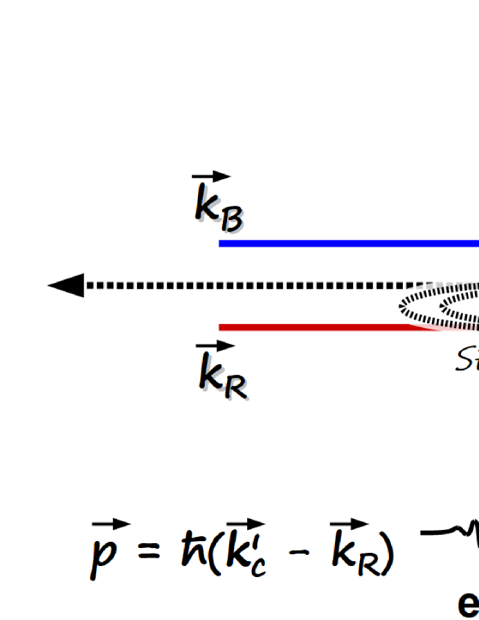
Figure 2: A beam configuration that produces diffusive stimulated transfers. The electron initially at rest receives a momentum kick from a stimulated transfer and its recoil energy is removed from the light field. By losing blue photons and gaining red photons, the spectrum of beam ${\boldsymbol{k}}$ shifts its intensity toward longer wavelengths. On average, the counter propagating beam ${\boldsymbol{k}}^{\prime}$ remains unaffected and the electron is heated by the interactions.

The spectral component ${\boldsymbol{k}}_{c}^{\prime}$ participates in two possible interactions. The first removes a photon from ${\boldsymbol{k}}_{B}$ and adds a photon via stimulated transfer into ${\boldsymbol{k}}_{c}^{\prime}$. A momentum kick $\Delta{\boldsymbol{p}}=\hbar({\boldsymbol{k}}_{B}-{\boldsymbol{k}}_{c}^{\prime})$ is transferred to the electron, which recoils and Doppler shifts the wavelength of the stimulated photon to $\lambda_{c}^{\prime}=\lambda_{B}+2\lambda_{e}$. The second possible interaction with ${\boldsymbol{k}}_{c}^{\prime}$ removes a photon from ${\boldsymbol{k}}_{c}^{\prime}$ and stimulates it into ${\boldsymbol{k}}_{R}$. The momentum kick $\Delta{\boldsymbol{p}}=\hbar({\boldsymbol{k}}_{c}^{\prime}-{\boldsymbol{k}}_{R})$ on the electron Doppler shifts the wavelength of the stimulated photon to $\lambda_{R}=\lambda_{c}^{\prime}+2\lambda_{e}$. The net wavelength shift between ${\boldsymbol{k}}_{B}$ and ${\boldsymbol{k}}_{R}$ is $4\lambda_{e}$, but since either one or the other possibility happens in a transfer event, the wavelength increases on average by $\Delta\lambda=2\lambda_{e}$ for each stimulated transfer. Beam ${\boldsymbol{k}}^{\prime}$ acts as a catalyst, as it remains mostly unaffected by the stimulated transfers produced by this configuration.

With a light field rich enough to contain the spectral components ${\boldsymbol{k}}_{B}$, ${\boldsymbol{k}}_{R}$, and ${\boldsymbol{k}}_{c}^{\prime}$, each stimulated transfer on a spectral component of the radiation produces a redshift $z_{0}$. Because ${\boldsymbol{k}}_{B}$ and ${\boldsymbol{k}}_{R}$ can be the spectral components of any beam, stimulated transfers produce a redshift on all radiation travelling through free electrons at a rate $\Gamma(n_{e})$. From Eq. (6) and (7), a wavelength shift of the entire spectrum occurs at the redshift rate

$$H_{z}\mbox{\,[s${}^{-1}$]}=z_{0}\times\Gamma(n_{e})=\alpha c\lambda_{e}^{2}\frac{\Phi}{\pi}\,n_{e}\approx 8.2\times 10^{-18}\,n_{e}$$ (8)

that only depends on the electron density. Despite the dependence of $z_{0}$ and $\Gamma(n_{e})$ on $\lambda$, the Stimulated Transfer redshift (STz) is independent of wavelength and preserves the spectral features of the spectrum at all wavelengths.

Because all energy transfers happen via stimulated emission, photons added to an already existing light beam acquire the direction of that beam, therefore causing no change of the beam’s wavefront properties. As a result, no blurring occurs and images of distant objects are maintained[16, 15] while the intensity of their spectrum is shifted toward longer wavelengths.

4 Discussion

In addition to the known mechanism of coronal heating,[13] Stimulated Transfer heating transfers a significant amount of energy to the corona. This is an important piece of the puzzle needed to solve the coronal heating problem that has been described as “perhaps the longest standing, most frustrating issue yet to be resolved in the solar physics community.”[17]

The simple model presented here is unstable to temperature perturbations for $T>0.25\mbox{\,MK}$ because the modelled radiative loss function decreases with temperature while Stimulated Transfer heating increases with temperature. To understand how stimulated transfers contribute to the high temperature of the solar corona, a detailed dynamical model will need to include solar limb darkening, energy transport, electron collisions, etc.

A spectral redshift of radiation propagating through free electrons is produced by Stimulated Transfer redshift (STz). Stimulated emission causes an energy loss that is a function of the column density of electrons without blurring the images of distant galaxies. With the simplification that $n_{e}$ is constant, integrating the energy loss Eq. (8) as a function of distance gives $z(D)=\exp\left[H_{z}D/c\right]-1$. This corresponds to the angular distance

$$d_{A}=(c/H_{z})\ln(1+z),$$ (9)

that has the same form as the equation published by Nernst.[18] Equating $H_{z}$ to $H_{0}=73.5\mbox{\,km/s/Mpc}$ taken from Ref. [19], Eq. (8) gives $n_{e}=0.29\mbox{\,/m${}^{3}$}$, in agreement with the measured value $n_{e}=0.22_{-0.13}^{+0.11}\mbox{\,/m${}^{3}$}$ of the electron density in the intergalactic medium.

Figure 3: Angular diameters of a 10-kpc-size object as a function of redshift. Dashed curve: based on $\Lambda$CDM. Dotted curve: based on Eq. (9) for a non-expanding cosmology with Tired-Light. Solid line: based on the Hubble constant $H_{0}$ and the angular distance as a linear function of $z$. Measured angular sizes of galaxies from JWST observations (red points) and some pre-JWST observations (black points) are overlapped with the curves. Figure copied from Lovyagin et al. (2023)[22]

From an observational point of view, Eq. (9) predicts the linear redshift-distance law found by Hubble[23] for small redshifts, and predicts a Hubble-Humason law up to large redshifts $z\approx 16$ as measured with JWST observations of galaxy diameters[22] as shown in Fig. 3.

To resolve the tensions in cosmology some authors propose a tired-light contribution to the redshift,[24, 25, 26] but the precise mechanism remains unspecified and additional parameters or assumptions are needed to obtain consistency with observations. By contrast, STz describes a mechanism that predicts astronomical observations from known physics.

The above derivation contains many simplifications, one of which is an equal number of photons in both the beam of interest ${\boldsymbol{k}}$ and the catalyst ${\boldsymbol{k}}^{\prime}$. In real situations, the number of photons differs and $n_{i}\neq n_{j}^{\prime}$ in Eq. (5) produces a variable transfer rate as a function of distance from the sources. As shown in the example of the solar corona, unbalanced values of $n_{i}$ and $n_{j}^{\prime}$ near light sources prevent a large number of stimulated transfers, even if the electron density is higher than the average value in the intergalactic medium. More detailed modelling is beyond the scope of this paper and will be published elsewhere.

5 Conclusions

A quantum calculation of momentum diffusion that includes terms usually considered negligible accurately describes momentum diffusion in the gradient force on free electrons. The photon-electron interaction, calculable from QED, has diffusive properties that increase the temperature of the electrons and removes energy from the light field. The effect is based on stimulated emission and maintains the directional properties of all light beams.

The calculated heating of electrons in a plasma illuminated by intense light is confirmed by measurements of the solar corona temperature that reaches millions of Kelvins.

Intersecting light beams lose energy to the electrons of the intergalactic medium, resulting in the shift of their spectral intensity toward longer wavelengths without blurring the images of distant objects. Photons are replaced by new photons of slightly less energy propagating in the same direction as the original beam. From the measured electron density in the intergalactic medium, the Stimulated Transfer redshift predicts a redshift-distance relationship that agrees with the Hubble-Humason law up to $z\approx 16$.

Stimulated transfers play an important role in astrophysical processes and observations, producing effects that support a very different interpretation of the universe. In light of all this, “cautiousness requires not to interpret too dogmatically the observed redshifts as caused by an actual expansion.”[27]

References

- [1] M.V. Fedorov, S.P. Goreslavsky, and V.S. Letokhov. Ponderomotive forces and stimulated Compton scattering of free electrons in a laser field. Phys. Rev. E, 55(1):1015–1027, 1997. doi: 10.1103/PhysRevE.55.1015.
- [2] R.J. Cook. Quantum-Mechanical Fluctuations of the Resonance-Radiation Force. Phys. Rev. Lett., 44(15):976–979, 1980. doi: 10.1103/PhysRevLett.44.976.
- [3] J.P. Gordon and A. Ashkin. Motion of atoms in a radiation trap. Physical Review A, 21(5):1606–1617, 1980. doi: 10.1103/PhysRevA.21.1606.
- [4] A.V. Gaponov and M.A. Miller. Potential Wells for Charged Particles in a High-Frequency Electromagnetic Field. J. Exptl. Theoret. Phys. (U.S.S.R.), 34:242–243, 1958. http://jetp.ras.ru.
- [5] C. Cohen-Tannoudji, J. Dupont-Roc, and G. Grynberg. Atom-Photon Interactions: Basic Processes and applications. WILEY-VCH Verlag GmbH & Co. KGaA, Weinheim, 2004.
- [6] W. Heitler. The Quantum Theory of Radiation. Oxford University Press, Ely House, London W. 1, third edition, 1954.
- [7] B.W. Shore, P. Meystre, and S. Stenholm. Is a quantum standing wave composed of two traveling waves? J. Opt. Soc. Am., B8(4):903–910, 1991. doi: 10.1364/JOSAB.8.000903.
- [8] H. Alfvén. On the solar corona. Arkiv för Matematik, Astronomi och Fysik, 27 A(25):1–23, 1941. https://ui.adsabs.harvard.edu.
- [9] A. Brynjolfsson. Redshift of photons penetrating a hot plasma,. arXiv:astro-ph/0401420, 2004.
- [10] R. Rosner, W.H. Tucker, and G.S. Vaiana. Dynamics of the Quiescent Solar Corona. The Astrophysical Journal, 220(2):643–665, 1978. doi: 10.1086/155949.
- [11] H.P. Warren and D.H. Brooks. The Temperature And Density Structure Of The Solar Corona. I. Observations Of The Quiet Sun With The EUV Imaging Spectrometer On HINODE. The Astrophysical Journal, 700(1):762–773, 2019. doi: 10.1088/0004-637X/700/1/762.
- [12] H. Morgan and J. Pickering. SITES: Solar Iterative Temperature Emission Solver for Differential Emission Measure Inversion of EUV Observations. Solar Phys, 294(10):1–23, 2019. doi: 10.1007/s11207-019-1525-4.
- [13] S.R. Cranmer and A.R. Winebarger. The Properties of the Solar Corona and Its Connection to the Solar Wind. Annu. Rev. Astron. Astrophys., 57(1):157–187, 2019. doi: 10.1146/annurev-astro-091918-104416.
- [14] L.E. Ashmore. Recoil Between Photons and Electrons Leading to the Hubble Constant and CMB. Galilean Electrodynamics, 17(Special Issue No. 3):53–57, 2006. https://www.galilean-electrodynamics.com.
- [15] J. Moret-Bailly. Propagation of light in low-pressure ionized and atomic hydrogen: application to astrophysics. IEEE Trans. Plasma Sci., 31(6):1215–1222, 2003. doi: 10.1109/TPS.2003.821476.
- [16] L. Marmet. Optical Forces as a Redshift Mechanism: the “Spectral Transfer Redshift”. In F. Potter, editor, 2nd Crisis in Cosmology Conference, CCC-2, volume 413 of Astronomical Society of the Pacific Conference Series, pages 268–276, San Francisco, CA, May 2009. Astronomical Society of the Pacific. http://aspbooks.org.
- [17] H. Gilbert. Advances in solar telescopes. Physics Today, 76(8):40–47, 2023. doi: 10.1063/PT.3.5292.
- [18] W. Nernst. Weitere Prüfung der Annahme eines stationären Zustandes im Weltall. Zeitschrift für Physik, 106:633–661, 1937. doi: 10.1007/BF01339902; translation in Apeiron 2(3) July 1995, http://redshift.vif.com/journal_archives.htm.
- [19] D. Brout et al. The Pantheon+ Analysis: Cosmological Constraints. ApJ, 938(2):110–133, 2022. doi: 10.3847/1538-4357/ac8e04.
- [20] L. Marmet. On the Interpretation of Spectral Red-Shift in Astrophysics: A Survey of Red-Shift Mechanisms - II. arXiv:1801.07582, 2018.
- [21] J. Baptista et al. Measuring the Variance of the Macquart Relation in Redshift–Extragalactic Dispersion Measure Modeling. ApJ, 965(1):57–67, 2024. doi: 10.3847/1538-4357/ad2705.
- [22] N. Lovyagin, A. Raikov, V. Yershov, and Y. Lovyagin. Cosmological Model Tests with JWST. Galaxies, 10(6):108–127, 2022. doi: 10.3390/galaxies10060108.
- [23] E. Hubble and M.L. Humason. The Velocity-Distance Relation among Extra-Galactic Nebulae. ApJ, 74:43–80, 1931. doi: 10.1086/143323.
- [24] M. López-Corredoira and L. Marmet. Alternative ideas in cosmology. Int. J. Mod. Phys. D, 31(8):2230014–1–37, 2022. doi: 10.1142/S0218271822300142; also arXiv:2202.12897.
- [25] R.P. Gupta. Testing CCC+TL Cosmology with Observed Baryon Acoustic Oscillation Features. ApJ, 964(1):55–62, 2024. doi: 10.3847/1538-4357/ad1bc6.
- [26] L. Shamir. An Empirical Consistent Redshift Bias: A Possible Direct Observation of Zwicky’s TL Theory. Particles, 7(3):703–716, 2024. doi: 10.3390/particles7030041.
- [27] F. Zwicky. Remarks on the Redshift from Nebulae. Phys. Rev., 48(10):802–806, 1935. doi: 10.1103/PhysRev.48.802.