1 Introduction

The consistency of standard least-squares estimates rely on covariates being uncorrelated with the additive noise; when this condition breaks down, the covariates are said to be endogenous. Instrumental variables (IV) provide an important class of methods for addressing this challenge. Since their introduction in the appendix of Wright’s book [46], IV methods have come to play a key role in semi-parametric statistics, econometrics, reinforcement learning, and causal inference. They exploit randomness in an external measurement, known as an instrument, in order to overcome endogeneity. Classical work on IV methods focused on their use for errors-in-variables [35], whereas Angrist and Krueger [4] popularized their use for answering causal questions. Econometric questions in which IV methods have proven valuable include understanding the economic returns of education [4, 11]; the effect of pre-trial detention on different outcomes [19, 28]; the consequences of serving in the Vietnam War for future earnings and mortality  [5, 3]; and the effects of C-sections on infant health outcomes [14], among others. Instrumental variables also arise in reinforcement learning, where they underlie the TD-learning family of algorithms (e.g., [40, 37, 24, 15]).

Given this wide range of applied uses, there is now a rich literature on the theoretical properties of instrumental variables. The papers [3, 22] provided an explicit causal interpretation of the IV estimate (or Wald estimator, to be precise) as the local average treatment effect. It is well-known that the IV estimator is a special case of the more general class of estimators known as generalized method of moments [32]. From this, the classical asymptotic theory of GMM estimators [21] thus also apply. Modern work in the theory of IV estimators has focused on the weak instrument setting [39, 7], where the correlation (i.e. strength) of the instrument with the covariate of interest is too small, relative to the sample size. In another line of work, there has been a focus on using LASSO [42] to address high-dimensional issues that can occur while using instrumental variables [9], or incorporating more modern techniques in machine learning under IV estimation [12], with mixed success [2].

The vast majority of this research has been asymptotic in nature. The references [21, 32] provide a classical $\sqrt{n}$-asymptotic analysis of instrumental variables through the central limit theorem. Yet it is well know that in modern statistical settings, this style of CLT analysis often breaks down. The weak instrument literature studies a specialized asymptotic regime that considers the ratios of normal approximations [7]. However recent work [48] has highlighted issues with the normal approximation used within the weak IV literature. In an effort to compare the finite-sample behavior of various procedures, researchers have turned towards higher-order asymptotic expansions and comparing these higher order terms with each other [33]. The paper [16] provides an asymptotic analysis of various types of IV estimators in the setting with many instruments and exogeneous covariates. In spite of all this, a non-asymptotic analysis of instrumental variables still remains lacking. One contribution of this work is the first instance of this style of analysis, to the best of our knowledge.

To further motivate our paper, as a practical application we consider the health effects of fine particulate matter (PM_2.5) exposure. The association between exposure to high levels of PM_2.5 and negative health outcomes such as mortality rates [26, 20], childhood asthma rates [27], cardiovascular issues in the elderly [10], and many other conditions, is well-known in the literature. However all of these have studied the association between exposure to PM_2.5 and health outcomes. There is a relatively recent line of work using causal inference/econometric methodology to analyze this connection, beginning with Pope [23]. The paper [36] uses air trajectory data as an instrument for PM_2.5; a related work [45] uses a differences-in-differences approach. Both studies draw conclusions consistent with previous studies on the effects of PM_2.5 exposure and increasing mortality rates. In the last few years alone, there have been many studies dedicated to analyzing the health effects of PM_2.5 exposure in various Asian nations, using atmospheric data as an instrument [47].

1.1 Our contributions

The main contribution of this paper is to provide some non-asymptotic insight into the behavior of the classical IV estimator, both in terms of its $\ell_{2}$-error, and in terms of linear functionals of the IV estimate. Moreover, in many settings, researchers often introduce exogeneous covariates; these covariates often are additional measurements used as features to improve the quality of our estimate but are nuisances in the sense that we are not interested in their effect on the response. We provide guarantees on the estimation of the component of interest in the presence of exogeneous covariates, which follows as a special case from our results on linear functionals.

Our first set of results (Theorems 1 and 2) are aimed at characterizing the rate at which the IV error converges to the asymptotic prediction. The terms in these bounds depend on various aspects of the problem, including the number of exogenous variables and the strength of endogeneity, and we illustrate our theoretical predictions via simulations on synthetic ensembles. Our second set of results, including Theorem 3 and Corollaries 1,  2 and 3, provide procedures for computing confidence intervals based on the data. These bounds involve adaptive correction factors to the classical asymptotic prediction based on the sandwich estimate. These results also lead us to a novel measure of the strength of an instrument.

Finally, to illustrate the use of our findings, we apply instrumental variables to analyze the effects of PM_2.5 exposure on negative health outcomes. For our paper, we have constructed a novel dataset based on various governmental sources to analyze this relationship. In our approach, we treat each individual census tract as a unit of observation, and consider aggregate measures of health outcomes for these census tracts. The data about PM_2.5 emissions are taken from the Public Health Tracking Network under the Centers for Disease Control and Prevention (CDC) [17]. We constructed an instrument based around wildfire exposure, taken from the National Interagency Fire Center [13]. The data for the exogeneous covariates, including information about the racial and demographic makeup, breakdown of employment by industry, log median wage, education, and much more is taken from the 2020 US Census, accessed via the IPUMS NHGIS [31]. The health outcomes of census tracts are obtained from the PLACES project conducted via the CDC [18].

1.2 Notation

For a vector $v\in\mathbb{R}^{d}$, we use $\big{\|}v\big{\|}_{2}$ to denote its Euclidean norm. For a matrix $\mathbf{A}\in\mathbb{R}^{d\times k}$, its spectral norm is given by

$$|\!|\!|\mathbf{A}|\!|\!|_{{2}}=\sup_{v\in\mathbb{R}^{k}}\frac{|v^{T}\mathbf{A}v|}{\big{\|}v\big{\|}_{2}^{2}},$$

and its maximum and minimum singular values by $\rho_{\text{max}}\big{(}\mathbf{A}\big{)}$ and $\rho_{\text{min}}\big{(}\mathbf{A}\big{)}$, respectively. We use $\textbf{I}_{d}\in\mathbb{R}^{d\times d}$ to denote the identity matrix of size $d$. We use $[n]$ to denote the set $\{1,2,\ldots n\}$. For a pair of symmetric matrices, we write $\mathbf{A}\succeq\mathbf{B}$ to mean that $\mathbf{A}-\mathbf{B}$ is positive semidefinite (PSD). For a matrix $\mathbf{A}\in\mathbb{R}^{d_{1}\times d_{2}}$, we use $\mathbf{A}^{T}$ to denotes its matrix transpose in $\mathbb{R}^{d_{2}\times d_{1}}$. We use $\overset{p}{\to}$ to denote convergence in probability, and $\rightsquigarrow$ to indicate convergence in distribution. Throughout the paper, we use $c_{0},c_{1},c_{2},\ldots$ as universal constants whose values may change from line to line.

1.3 Paper organization

The remainder of the paper is organized as follows. We begin in Section 2 with background on the linear IV estimator, and its extension to exogenous variables. In Section 3, we turn to the main results of the paper, including non-asymptotic bounds for the standard IV estimate (Theorem 1 in Section 3.1), along with bounds for linear functions allowing for exogenous covariates (Theorem 2 in Section 3.2). Section 3.3 is devoted to non-asymptotic and fully computable confidence intervals. In Section 4, we explore the applied consequences of our results, including a numerical study of our confidence intervals, along with an applied study of IV methods for assessing the effects of PM2.5 pollution. We conclude with a discussion in Section 5.

2 Background

Here we provide a very brief introduction to the theory of instrumental variables; see the sources [6, 32] for more details. Section 2.1 introduces the standard instrumental variable setup, whereas Section 2.2 introduces the notion of exogeneous covariates.

2.1 Standard instrumental variables

Consider a scalar response $y$ and covariate vector $X\in{}^{d}$ linked via the linear model

$$y =\langle X,\,\beta^{*}\rangle+\varepsilon,$$ (1a)

where $$\varepsilon \beta^{*}\in{}^{d} \varepsilon \mathbb{E}[X\varepsilon]=0$$ is an additive noise term. Ordinary least-squares (OLS) is a standard way of estimating the unknown vector of parameters. In the classical formulation, the noise is assumed to be a zero-mean random variable such that . This lack of correlation ensures consistency of the OLS estimate.

Instrumental variables are designed to handle cases in which the covariate vector $X$ and noise term $\varepsilon$ are correlated. Such dependence can arise for various reasons, with an archetypal example being mis-specification in a linear model. As a simple but concrete illustration, consider a linear model with covariates $(X,u)\in{}^{d}\times\real$ linked to the response $y$ via

$$y =\langle X,\,\beta^{*}\rangle+u\alpha^{*}+w.$$ (1b)

When this linear model is well-specified, then we are guaranteed to have the orthogonality condition $\mathbb{E}[(X,u)w]=0$. However, suppose that the additional covariate $u$ is not observed (and hence not modeled); in this case, it is natural to view the model (1b) as a version of the $X$-based model (1a) with the augmented noise term $\varepsilon\coloneq u\alpha^{*}+w$. An easy calculation gives $\mathbb{E}[X\varepsilon]=\mathbb{E}[Xu]\alpha^{*}$, so that whenever $\alpha^{*}\neq 0$, any correlation between $X$ and $u$ will render $X$ and $\varepsilon$ correlated as well. In the econometrics literature, this phenomenon is known as omitted variable bias.

Returning to the original model (1a), a vector $Z\in{}^{d}$ is said to be an instrument if

$$\mathbb{E}[Z\varepsilon]\stackrel{{\scriptstyle(\star)}}{{=}}0,\quad\text{and the matrix $\mathbf{\Gamma}\coloneq\mathbb{E}\left[ZX^{T}\right]$ is full rank.}$$ (2)

Condition ($\star$) is known as the clean instrument condition, whereas the full-rank condition is known as the fully correlated requirement. Given an instrument $Z$, a straightforward calculation using the linear model (1a) shows that $\beta^{*}$ satisfies

$$\mathbb{E}[Zy]=\mathbb{E}[ZX^{T}]\beta^{*}=\mathbf{\Gamma}\beta^{*},\quad\mbox{or equivalently $\beta^{*}=\mathbf{\Gamma}^{-1}\mathbb{E}[Zy]$,}$$ (3)

where the second equation uses the full rank condition. While the expectations defining this relation are unknown, given i.i.d. samples $\{(y_{i},X_{i},Z_{i})\}_{i=1}^{n}$, we can use the plug-in principle to form the estimate

$$\widehat{\beta}=\left(\frac{1}{n}\sum_{i=1}^{n}Z_{i}X^{T}_{i}\right)^{-1}\left(\frac{1}{n}\sum_{i=1}^{n}y_{i}Z_{i}\right),$$ (4)

which is the standard instrumental variable estimator.

Under i.i.d. sampling and regularity conditions, the standard asymptotic argument shows that

$$\sqrt{n}(\widehat{\beta}-\beta^{*})\rightsquigarrow\mathcal{N}(0,\mathbf{\Gamma}^{-1}\mathbf{\Sigma}\mathbf{\Gamma}^{-T})$$ (5)

where $\mathbf{\Gamma}\coloneq\mathbb{E}[ZX^{T}]$ and $\mathbf{\Sigma}\coloneq\mathbb{E}[\varepsilon^{2}ZZ^{T}]$.

2.2 Instrumental variables and exogenous covariates

In most practical settings, in addition to a set of endogenous covariates $X\in{}^{d}$, we also have a vector exogenous covariates $W\in\mathbb{R}^{p}$, leading to the augmented model

$$y =\langle X,\,\beta^{*}\rangle+\langle W,\,\alpha^{*}\rangle+\varepsilon_{i},$$ (6)

with the moment restrictions $\mathbb{E}[Z\varepsilon]=0$ and $\mathbb{E}[W\varepsilon]=0$. Here our primary goal remains to estimate $\beta^{*}$, and the additional covariates $W$ are introduced to avoid mis-specification and/or reduce the variability in our estimate of $\beta^{*}$. The associated parameter vector $\alpha^{*}$ can be viewed as a “nuisance”; it is not of interest per se, but needs to be handled so as to obtain a better estimate of $\beta^{*}$.

Let us now describe how the problem of estimating $\beta^{*}$ can be reformulated as one of estimating a linear function of the parameter vector in a “lifted” standard IV estimate. We define the full parameter vector $\theta^{*}\coloneq\begin{bmatrix}\beta^{*}\\ \alpha^{*}\end{bmatrix}\in{}^{d+p}$, along with the lifted covariate and instrument vectors

$$X^{\prime}\coloneq\begin{bmatrix}X\\ W\end{bmatrix},\quad\text{and}\quad Z^{\prime}\coloneq\begin{bmatrix}Z\\ W\end{bmatrix}.$$

With this notation, our original model can be written more compactly as $y=\langle X^{\prime},\,\theta^{*}\rangle+\varepsilon$. Note that we have have $\mathbb{E}[Z^{\prime}\varepsilon]=0$ by construction, so that the lifted vector $Z^{\prime}\in{}^{p+d}$ is a valid instrument. Consequently, we can compute the standard IV estimate $\widehat{\theta}$ using samples of the triples $(y_{i},X^{\prime}_{i},Z^{\prime}_{i})$, and we can recover the estimate $\widehat{\beta}$ of interest as $\widehat{\beta}=\mathbf{U}^{T}\widehat{\theta}$, where $\mathbf{U}^{T}\coloneq\begin{bmatrix}\mathbf{I}_{d}&\mathbf{0}_{p}\end{bmatrix}$. We give results on the estimation of such linear functions of an IV estimate in Theorem 2 and Corollary 1 to follow in the sequel.

3 Main results

In this section we present the main theorems of this paper. Section 3.1 is devoted to non-asymptotic guarantees for the standard instrumental variable estimator. Section 3.2 provides extensions to estimation in the presence of exogeneous covariates, which amounts to estimating a linear mapping of the original IV estimate. Finally, in Section 3.3, we turn to the construction of confidence intervals that can be equipped with non-asymptotic guarantees.

3.1 Non-asymptotic bounds for standard IV

We begin with some finite-sample results for the standard IV estimate without exogenous covariates. In particular, suppose that we observe triples $\{(y_{i},X_{i},Z_{i})\}_{i=1}^{n}$ such that

$$y_{i}=\langle X_{i},\,\beta^{*}\rangle+\varepsilon_{i}\qquad\mbox{with $\mathbb{E}[Z_{i}\varepsilon_{i}]=0$.}$$ (7)

Defining the matrix $\mathbf{\Gamma}_{n}\coloneq\frac{1}{n}\sum_{i=1}^{n}\mathbb{E}[Z_{i}X_{i}^{T}]$, we assume that it is invertible, as is necessary for the instrument sequence $\{Z_{i}\}_{i=1}^{n}$ to be useful. Apart from this condition, we impose no other distributional conditions on the covariates $\{X_{i}\}_{i=1}^{n}$.

Our main assumptions are imposed on the zero-mean random vectors $Z_{i}\varepsilon_{i}\in{}^{d}$: in particular, we require the existence of a finite constant $b$ such that

$$\{Z_{i}\varepsilon_{i}\}_{i=1}^{n}$$ is an independent sequence of zero-mean variables, and (8a)

$$\|\mathbf{\Gamma}_{n}^{-1}(Z_{i}\varepsilon_{i})\|_{2}\leq b\qquad\mbox{almost surely for each $i=1,\ldots,n$.}$$ (8b)

We use the independence (8a) and $b$-boundedness conditions (8b) in order to establish tail bounds on sums of the terms $\mathbf{\Gamma}_{n}^{-1}(\varepsilon_{i}Z_{i})$. We note that in many practical settings of interest, the instruments $Z_{i}$ and noise $\varepsilon_{i}$ are bounded, in which case the $b$-boundedness condition holds. Moreover, we note that that it is straightforward (although requiring more technical analysis) to extend our results to unbounded random vectors with reasonable tail behavior.

3.1.1 A non-asymptotic bound

Our result involves the matrices

$$\widehat{\mathbf{\Gamma}}_{n}\coloneq\frac{1}{n}\sum_{i=1}^{n}Z_{i}X^{T}_{i},\quad\mbox{and}\quad\mathbf{\Gamma}_{n}\coloneq\mathbb{E}[\widehat{\mathbf{\Gamma}}_{n}]\equiv\frac{1}{n}\sum_{i=1}^{n}\mathbb{E}[Z_{i}X_{i}^{T}],$$ (9a)

$$\widetilde{\mathbf{\Sigma}}_{n}\coloneq\frac{1}{n}\sum_{i=1}^{n}\varepsilon_{i}^{2}Z_{i}Z_{i}^{T},\quad\mbox{and}\quad\mathbf{\Sigma}_{n}\coloneq\mathbb{E}[\widetilde{\mathbf{\Sigma}}_{n}]\equiv\frac{1}{n}\sum_{i=1}^{n}\mathbb{E}[\varepsilon_{i}^{2}Z_{i}Z_{i}^{T}].$$ (9b)

We also define the zero-mean random vector

$$G_{n} \coloneq\frac{1}{\sqrt{n}}\sum_{i=1}^{n}\mathbf{\Gamma}_{n}^{-1}Z_{i}\varepsilon_{i},$$ (10)

and observe that we have $\mathrm{cov}(G_{n})=\mathbf{\Gamma}_{n}^{-1}\mathbf{\Sigma}_{n}\mathbf{\Gamma}_{n}^{-T}$ by independence of the sequence $\{Z_{i}\varepsilon_{i}\}_{i=1}^{n}$. Thus, given the classical asymptotic behavior (5) of the standard IV estimate under i.i.d. sampling, it is reasonable to expect that the IV estimate—under the more relaxed distribution assumptions that we impose—should satisfy

$$\sqrt{n}\;\mathbb{E}\|\widehat{\beta}-\beta^{*}\|_{2} \approx\mathbb{E}\|G_{n}\|_{2}$$ (11)

for all suitably large $n$. The goal of this section is to make this intuition precise: we prove an upper bound, valid for any sample size $n$, in which this quantity is the leading order term.

In order to establish a non-asymptotic bound of this type, we need to introduce a quantity that measures the deviation between the population matrix $\mathbf{\Gamma}_{n}$ and its empirical counterpart $\widehat{\mathbf{\Gamma}}_{n}$ from equation (9a). In particular, we define

$$\gamma_{n}(\mathbf{\Gamma}_{n})\coloneq|\!|\!|\widehat{\mathbf{\Gamma}}_{n}^{-1}\mathbf{\Gamma}_{n}-\mathbf{I}_{d}|\!|\!|_{{2}}$$ (12)

where $|\!|\!|\cdot|\!|\!|_{{2}}$ denotes the $\ell_{2}$-operator norm, or maximum singular value. As we discuss below, in typical settings, we expect that $\gamma_{n}(\mathbf{\Gamma}_{n})$ scales as $\sqrt{\frac{d}{n}}$ with the dimension $d$ and sample size $n$.

With this set-up, we are now ready to state our first main result:

Theorem 1.

Consider the model (7) such that the sequence $\{Z_{i}\varepsilon_{i}\}_{i=1}^{n}$ satisfies the independence (8a) and $b$-boundedness conditions (8b). For any $\delta\in(0,1)$, we have

$$\big{\|}\widehat{\beta}-\beta^{*}\big{\|}_{2} \leq\frac{1+\gamma_{n}(\mathbf{\Gamma}_{n})}{\sqrt{n}}\left\{\mathbb{E}\|G_{n}\|_{2}+\sqrt{2\log(\tfrac{1}{\delta})\mathbb{E}|\!|\!|\mathbf{\Gamma}_{n}^{-1}\widetilde{\mathbf{\Sigma}}_{n}\mathbf{\Gamma}_{n}^{-T}|\!|\!|_{{2}}}+\frac{3b\log(\tfrac{1}{\delta})}{\sqrt{n}}\right\}$$ (13)

with probability at least $1-\delta$.

We prove this result in Appendix A. The proof involves a careful decomposition of the error in the IV estimate, and then reducing the problem to studying the supremum of a certain empirical process.

Some remarks:

Let us make a few comments so as to interpret the bound (13). Beginning with the leading term, by Jensen’s inequality, we have

$$\mathbb{E}\|G_{n}\|_{2} \leq\sqrt{\mathbb{E}\|G_{n}\|_{2}^{2}}\;=\;\sqrt{\operatorname{Tr}(\mathbf{\Gamma}_{n}^{-1}\mathbf{\Sigma}_{n}\mathbf{\Gamma}_{n}^{-T})},$$

where the last step uses the fact that $\mathrm{cov}(G_{n})=\mathbf{\Gamma}_{n}^{-1}\mathbf{\Sigma}_{n}\mathbf{\Gamma}_{n}^{-T}$ by construction. Given the classical asymptotic relation (5), the appearance of this covariance matrix is to be expected.

Turning to the second term, let us first consider the uni-variate setting ($d=1$). In this case, we have $\mathbb{E}|\!|\!|\mathbf{\Gamma}_{n}^{-1}\widetilde{\mathbf{\Sigma}}_{n}\mathbf{\Gamma}_{n}^{-T}|\!|\!|_{{2}}=\operatorname{Tr}(\mathbf{\Gamma}_{n}^{-1}\mathbf{\Sigma}_{n}\mathbf{\Gamma}_{n}^{-T})$ so the bound simplifies to

$$\big{\|}\widehat{\beta}-\beta^{*}\big{\|}_{2}\leq\frac{1+\gamma_{n}(\mathbf{\Gamma}_{n})}{\sqrt{n}}\left(\big{(}1+\sqrt{2\log(\tfrac{1}{\delta}})\big{)}\cdot\sqrt{\operatorname{Tr}(\mathbf{\Gamma}_{n}^{-1}\mathbf{\Sigma}_{n}\mathbf{\Gamma}_{n}^{-T})}+\frac{3b\log(\tfrac{1}{\delta})}{\sqrt{n}}\right).$$

For an arbitrary dimension $d$, since $\mathbb{E}|\!|\!|\mathbf{\Gamma}_{n}^{-1}\widetilde{\mathbf{\Sigma}}_{n}\mathbf{\Gamma}_{n}^{-T}|\!|\!|_{{2}}\leq\operatorname{Tr}(\mathbf{\Gamma}_{n}^{-1}\mathbf{\Sigma}_{n}\mathbf{\Gamma}_{n}^{-T})$, this inequality is always valid. However, in high-dimensional settings, the trace of a matrix can be be considerably larger—up to factor of $d$—than its spectral norm, so that the bound that we have established can be much sharper.

Finally, let us consider the pre-factor $\gamma_{n}(\mathbf{\Gamma}_{n})=|\!|\!|\widehat{\mathbf{\Gamma}}_{n}^{-1}\mathbf{\Gamma}_{n}-\mathbf{I}_{d}|\!|\!|_{{2}}$. In a classical analysis—viewing the dimension $d$ as fixed—this term scales as $1/\sqrt{n}$ so that we have $1+\gamma_{n}(\mathbf{\Gamma}_{n})=1+O(1/\sqrt{n})$. Thus, as $n$ tends to infinity, other problem parameters fixed, our bound matches the heuristic prediction (11) that motivated our analysis.

3.1.2 Numerics via the non-asymptotic lens

As noted earlier, our main interest is not re-capturing the asymptotic prediction, but rather understanding non-asymptotic aspects of the IV estimate. In order to highlight some non-asymptotic predictions of Theorem 1, it is helpful to perform simulations on synthetic ensembles designed to reveal certain behavior. In particular, here we explore the effects of two parameters that can vary: (i) the degree of endogeneity; and (ii) the number of instruments $d$.

Degree of endogeneity:

We begin by describing a simple ensemble to allows us to investigate the effect of varying endogeneity. Suppose that we generate covariate vectors $X\in{}^{d}$ that are related to the instrument $Z\in{}^{d}$ and additive noise $\varepsilon\in\real$ via the equation

$$X =\alpha Z+\eta\varepsilon\bf{1}_{d}+\nu W.$$ (14)

Here $W\sim\mathcal{N}(0,\mathbf{I}_{d})$ is a second source of noise, independent of the pair $(Z,\varepsilon)$, and ${\bf{1}}_{d}\in{}^{d}$ denotes a vector of all-ones. By construction, we have $\mathbb{E}[X\varepsilon]=\eta{\bf{1}}_{d}$, so that parameter $\eta$ controls the degree of endogeneity.

In order to study the effect of increasing endogeneity, we study ensembles with fixed instrument strength $\alpha=1$ and noise level $\nu=0$, and endogeneity level $\eta$ varying over the interval $[0,3.0]$. With this set-up, the setting $\eta=0$ leads to ensembles with $X=Z$, in which case the IV estimate reduces to the OLS estimate. Increasing $\eta>0$ leads to problems where $X$ is endogenous, with the parameter $\eta$ a measure of its strength. We constructed ensembles in dimension $d=5$ and parameters chosen to ensure that the asymptotic rescaled MSE $n\mathbb{E}\|\widehat{\beta}-\beta^{*}\|_{2}^{2}$ was equal to $1$.

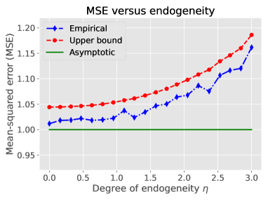
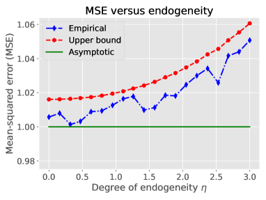
(a) $n=400$		(b) $n=1024$

Figure 1: Plot of the rescaled mean-squared error (MSE) $n\>\mathbb{E}\|\widehat{\beta}-\beta^{*}\|_{2}^{2}$ versus the degree of endogeneity $\eta$. Experiments were performed on ensembles from the generative model (14) with dimension $d=5$, and sample sizes $n=400$ and $n=1024$ in panels (a) and (b), respectively, with the parameter $\eta$ controlling the degree of endogeneity. For each ensemble, the asymptotic rescaled MSE was equal to $1$, as marked in a solid green line. The empirical MSE was estimated on the basis of $M=30000$ Monte Carlo trials, whereas the theoretical upper bound was computed using the $1+\gamma_{n}(\mathbf{\Gamma}_{n})$ correction to the leading term in Theorem 1.

Figure 1 plots the rescaled MSE $n\mathbb{E}\|\widehat{\beta}-\beta^{*}\|_{2}^{2}$ versus the endogeneity parameter $\eta$ for two different sample sizes ($n=400$ in panel (a), and $n=1024$ in panel (b)). Note that the discrepancy between the asymptotic prediction and the empirical MSE of the IV estimate (estimated by Monte Carlo trials) increases as $\eta$ grows, and the theoretical upper bound from Theorem 1 tracks this behavior.

Growing numbers of instruments:

In applications of IV, it can be the case that the number of instruments $d$ is relatively “large” compared to the sample size $n$, in which case the asymptotic predictions might be inaccurate. Let us explore some dimensional effects in the context of Theorem 1. We begin by observing that under mild conditions on the pairs $(X_{i},Z_{i})$, standard random matrix theory (cf. Chapter 5 in the book [44]) can be used to show that

$$\gamma_{n}(\mathbf{\Gamma}_{n})=|\!|\!|\widehat{\mathbf{\Gamma}}_{n}^{-1}\mathbf{\Gamma}_{n}-\mathbf{I}_{d}|\!|\!|_{{2}}\asymp\sqrt{\tfrac{d}{n}}$$

with high probability. For problem ensembles with this behavior, we we would expect that the MSE should converge to the asymptotic prediction for $(n,d)$-sequences such that $\tfrac{d}{n}\rightarrow 0$.

Figure 2: Plot of the rescaled mean-squared error (MSE) $(n/d)\mathbb{E}\|\widehat{\beta}-\beta^{*}\|_{2}^{2}$ versus the sample size $n$ for ensembles with the dimension $d_{n}$ growing as $d_{n}=\lceil n^{0.30}\rceil$. The empirical MSE was estimated on the basis of $M=2000$ Monte Carlo trials, whereas the theoretical upper bound was computed using the $1+\gamma_{n}(\mathbf{\Gamma}_{n})$ correction to the leading term in Theorem 1.

In order to verify this prediction, we generated $(X,Z)$ pairs from the model (14) with $\alpha=\eta=\nu=1$; the noise variable $\varepsilon$ being standard Gaussian; and the instrument $Z\in{}^{d}$ with i.i.d. Rademacher entries (equiprobable random signs in $\{-1,+1\}$). We studied ensembles parameterized by the pair $(n,d)$, and let the number of instruments grow as $d_{n}=\lceil n^{0.30}\rceil$. As shown in Figure 2, both the bound from Theorem 1 and the empirical MSE of the IV estimator converge to the asymptotic prediction under this form of high-dimensional scaling.

3.2 Bounds for linear functions and exogenous covariates

Recall from Section 2.2 the more general set-up in which the linear model includes a combination of endogenous covariates $X\in{}^{d}$ and exogenous covariates $W\in{}^{p}$, and our goal is to estimate the parameters associated with the endogenous covariates. In terms of the sampling model, suppose that we observe triples $(y_{i},X_{i},W_{i},Z_{i})$ from the linear model

$$y_{i} =\langle X_{i},\,\beta^{*}\rangle+\langle W_{i},\,\alpha^{*}\rangle+\varepsilon_{i},\qquad\mbox{such that $\mathbb{E}[Z_{i}\varepsilon_{i}]=0$ and $\mathbb{E}[W_{i}\varepsilon_{i}]=0$.}$$ (15)

As described in  Section 2.2, the problem of estimating $\beta^{*}$ can be reformulated as an instance of estimating a linear mapping of the parameter vector in a standard IV model. We recall the notation

$$\theta^{*}\coloneq(\beta^{*},\alpha^{*}),\quad X^{\prime}_{i}\coloneq(X_{i},W_{i}),\quad\mbox{and}\quad Z^{\prime}_{i}\coloneq(Z_{i},W_{i}).$$

Using this shorthand, we have a more compact reformulation of our problem: we observe triples $(y_{i},X^{\prime}_{i},Z^{\prime}_{i})$ such that

$$y_{i} =\langle X^{\prime}_{i},\,\theta^{*}\rangle+\varepsilon_{i},\qquad\mbox{such that $\mathbb{E}[Z^{\prime}_{i}\varepsilon_{i}]=0$.}$$ (16a)

The IV estimate is given by $$\widehat{\theta}=(\frac{1}{n}\sum_{i=1}^{n}Z^{\prime}_{i}(X^{\prime}_{i})^{T})^{-1}\sum_{i=1}^{n}Z^{\prime}_{i}y_{i} \beta^{*}=\begin{bmatrix}\mathbf{I}_{d}&\mathbf{0}_{p}\end{bmatrix}\theta^{*} \mathbf{I}_{d} d \mathbf{0}_{p} p$$, and our goal is to estimate the parameter , where denotes a -dimensional identity matrix, and denotes a -dimensional matrix of zeroes.

This problem is special case of estimating the quantity $\mathbf{U}^{T}\theta^{*}$ for some matrix $\mathbf{U}\in{}^{D\times k}$ with $D\coloneq d+p$. In other applications, we might be interested in estimating a single co-ordinate of $\theta^{*}$, so that $\mathbf{U}\in{}^{D}$ is a column vector. The theory below encompasses all of these cases.

3.2.1 A non-asymptotic bound

With a slight abuse of notation, we use $(\mathbf{\Gamma}_{n},\widehat{\mathbf{\Gamma}}_{n})$ and $(\mathbf{\Sigma}_{n},\widetilde{\mathbf{\Sigma}}_{n})$ to denote the population-empirical matrices defined as in equations (9a) and (9b), with the pair $(X_{i},Z_{i})$ replaced by $(X^{\prime}_{i},Z^{\prime}_{i})$. In terms of tail conditions on the random vectors, we impose the following $b$-boundedness conditions

$$\|\mathbf{\Gamma}_{n}^{-1}(Z^{\prime}_{i}\varepsilon_{i})\|_{2}\leq b,\quad\mbox{and}\quad\|\mathbf{U}^{T}\mathbf{\Gamma}_{n}^{-1}(Z^{\prime}_{i}\varepsilon_{i})\|_{2}\leq b$$ (16b)

almost surely for each $i=1,\ldots,n$. As noted earlier, these assumptions could be relaxed to sub-Gaussian tail conditions, at the expense of more complicated arguments and/or truncation arguments.

Recall from equation (10) the random vector $G_{n}\coloneq\frac{1}{\sqrt{n}}\sum_{i=1}^{n}\mathbf{\Gamma}_{n}^{-1}Z_{i}\varepsilon_{i}$. For a general matrix $\mathbf{A}\in{}^{D\times k}$, we define the functional

$$\Psi_{n}(\mathbf{A};\delta) \coloneq\mathbb{E}[\|\mathbf{A}^{T}G_{n}\|_{2}]+\sqrt{2\log(\tfrac{2}{\delta})\mathbb{E}|\!|\!|\mathbf{A}^{T}\mathbf{\Gamma}_{n}^{-1}\widetilde{\mathbf{\Sigma}}_{n}\mathbf{\Gamma}_{n}^{-T}\mathbf{A}|\!|\!|_{{2}}}+\frac{3b\log(\tfrac{2}{\delta})}{\sqrt{n}}$$ (17)

Our main result involves this functional with $\mathbf{A}=\mathbf{U}$ in the leading order term, and $\mathbf{A}=\mathbf{I}_{D}$ in the second-order term.

Theorem 2.

Consider the model (16a), and suppose that the sequence $\{Z^{\prime}_{i}\varepsilon_{i}\}_{i=1}^{n}$ is independent and satisfies the $(\mathbf{U},b)$-boundedness condition (16b). Then for any $\delta\in(0,1)$, the IV estimate $\widehat{\theta}$ satisfies the bound

$$\big{\|}\mathbf{U}^{T}(\widehat{\theta}-\theta^{*})\big{\|}_{2} \leq\frac{1}{\sqrt{n}}\Psi_{n}(\mathbf{U};\delta)+\frac{|\!|\!|\mathbf{U}^{T}(\widehat{\mathbf{\Gamma}}_{n}^{-1}\mathbf{\Gamma}_{n}-\mathbf{I}_{d})|\!|\!|_{{2}}}{\sqrt{n}}\Psi_{n}(\mathbf{I}_{D};\delta)$$ (18)

with probability at least $1-\delta$.

See Appendix A for a proof of this result.

We begin by observing that this claim is the natural generalization of Theorem 2 on the standard IV estimate. In particular, if we set $\mathbf{U}=\mathbf{I}_{D}$, then the bound (18) reduces to

$$\big{\|}\widehat{\theta}-\theta^{*}\big{\|}_{2} \leq\frac{1+|\!|\!|\widehat{\mathbf{\Gamma}}_{n}^{-1}\mathbf{\Gamma}_{n}-\mathbf{I}_{d}|\!|\!|_{{2}}}{\sqrt{n}}\;\Psi_{n}(\mathbf{I}_{D};\delta),$$

which is the statement of Theorem 2 (with slightly altered notation).

Theorem 2 makes distinct predictions when $\mathbf{U}$ is not the identity. Concretely, suppose that $\mathbf{U}\equiv u\in{}^{D}$ is a vector, and introduce the shorthand

$$\mathbf{L}_{n} \coloneq\mathbf{\Gamma}_{n}^{-1}\mathbf{\Sigma}_{n}\mathbf{\Gamma}_{n}^{-T}$$ (19a)

for the relevant covariance matrix. The leading term in $$\Psi_{n}(u;\delta) \mathbb{E}|u^{T}G_{n}|\leq\sqrt{u^{T}\mathbf{L}_{n}u} \Psi_{n}(\mathbf{I}_{D};\delta) \mathbb{E}\|G_{n}\|_{2}\leq\sqrt{\operatorname{Tr}(\mathbf{L}_{n})}$$ then can be bounded as , whereas the leading order term in can be bounded as . Consequently, disregarding the other terms in the result, we have an approximate bound of the form

$$\sqrt{n}\big{|}\langle u,\,\widehat{\theta}-\theta^{*}\rangle\big{|} \precsim\sqrt{u^{T}\mathbf{L}_{n}u}+\|u^{T}(\widehat{\mathbf{\Gamma}}_{n}^{-1}\mathbf{\Gamma}_{n}-\mathbf{I}_{d})\|_{2}\sqrt{\operatorname{Tr}(\mathbf{L}_{n})}.$$ (19b)

The leading term with $u^{T}\mathbf{L}_{n}u$ is as we expect, given the asymptotic behavior under classical scaling. As for the second term, since we expect that $\widehat{\mathbf{\Gamma}}_{n}$ becomes close to $\mathbf{\Gamma}_{n}$ as $n$ increases, the pre-factor in front of the second term will become negligible for large $n$.

However, in the non-asymptotic regime, when this term is still non-negligible, the bound contains a quantity proportional to $\sqrt{\operatorname{Tr}(\mathbf{L}_{n})}$. Note that this trace quantity will typically be much larger—often by a dimension-dependent factor—than the scalar $\sqrt{u^{T}\mathbf{L}_{n}u}$. Below we undertake some careful numerical simulations to show that, at least in finite samples, the IV error itself—and not just our bound on it—also exhibits a dependence on this trace term.

3.2.2 Some numerical studies

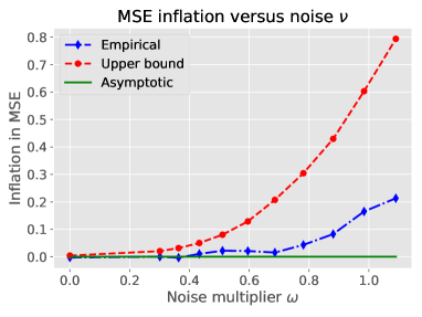
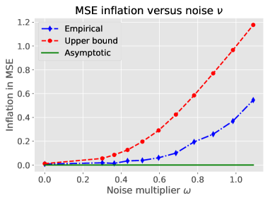
(a) $n=400$		$n=1024$

Figure 3: Plots of the log increase in mean-square error (MSE) versus the noise parameter $\omega$ for ensembles in dimension $d$ and $n=256$ with the error matrix $\mathbf{L}_{n}\equiv\mathbf{L}_{n}(\omega)$ in equation (20). (a) Simulations with $\nu=0.50$. (b) Simulations with $\nu=1.0$. In both panels, solid green lines correspond to the asymptotic log MSE (equal to zero by construction); dash-dot blue lines correspond to the IV empirical MSE estimated by $M=2500$ Monte Carlo trials; and dashed red lines correspond to the predictions from equation (19b).

Recalling the definition (19a) of the matrix $\mathbf{L}_{n}$ and following discussion, let us describe some numerical studies that reveal how the IV estimate error itself depends on the trace term $\operatorname{Tr}(\mathbf{L}_{n})$. In order to do so, we construct an ensemble of problems, parameterized by a weight $\omega\geq 0$, for which

$$\mathbf{L}_{n} =\mathbf{\Gamma}_{n}^{-1}\mathbf{\Sigma}_{n}\mathbf{\Gamma}_{n}^{-1}=\operatorname{diag}\big{(}1,\ldots,\omega,\ldots,\omega\big{)}.$$ (20)

See Appendix D for the details of this construction.

Letting $u=e_{1}$ be the standard basis vector with a single one in position $1$, we then have $u^{T}\mathbf{L}_{n}u=1$ for any value of $\omega$, whereas $\operatorname{Tr}(\mathbf{L}_{n})=1+(d-1)\omega$. Consequently, the leading term in our bound (19b) is independent of $\omega$, whereas the higher-order trace term grows linearly in $\omega$. In summary, then, the asymptotic prediction for the $n$-rescaled MSE is equal to $1$ for all values of $\omega$, whereas our theory predicts that the higher-order terms should scale with $\omega$.

In order to study the correspondence between our non-asymptotic predictions and the IV error in practice, we simulated from this ensemble in dimension $d$ with sample size $n=256$, instrument strength $\alpha=1$, endogeneity level $\eta=0.10$, and the parameter $\omega$ ranging over the unit interval $[0,1]$. We did so for different levels of noise level $\nu\in\{0.5,1.0\}$. For each setting of the parameters, we estimated the MSE of the IV estimate useful based on $M=2500$ Monte Carlo trials. Figure 3 gives plots of the log increase in mean-squared error (MSE) beyond the asymptotic prediction for both the actual IV estimate (dash-dot blue lines), and our theoretical upper bound (dashed red lines). Panels (a) and (b) correspond to noise levels $\nu=0.50$ and $\nu=1.0$, respectively. Consistent with the theory, the empirical MSE increases with the noise multiplier $\omega$ that parameterize the structure of the matrix $\mathbf{L}_{n}\equiv\mathbf{L}_{n}(\omega)$.

3.3 Computable confidence intervals

We now turn to the task of devising non-asymptotic and data-dependent confidence intervals on the error $\widehat{\beta}-\beta^{*}$ in the IV estimate. In particular, we derive bounds that depend on the empirical matrix $\widehat{\mathbf{\Gamma}}_{n}=\frac{1}{n}\sum_{i=1}^{n}Z_{i}X_{i}^{T}$, along with a standard estimate of the matrix $\mathbf{\Sigma}_{n}\coloneq\frac{1}{n}\sum_{i=1}^{n}\mathbb{E}[\varepsilon_{i}^{2}Z_{i}Z_{i}^{T}]$—namely, the random matrix

$$\widehat{\mathbf{\Sigma}}_{n} \coloneq\frac{1}{n-1}\sum_{i=1}^{n}\widehat{\varepsilon}^{2}_{i}Z_{i}Z_{i}^{T}$$ (21a)

where $$\widehat{\varepsilon}_{i}\coloneq y_{i}-\langle X_{i},\,\widehat{\beta}\rangle \widehat{\mathbf{\Gamma}}_{n}^{-1}\widehat{\mathbf{\Sigma}}_{n}\widehat{\mathbf{\Gamma}}_{n}^{-T}$$ are the residuals associated with the IV estimate. Combining these ingredients yields the standard “sandwich” estimate for the asymptotic covariance.

In addition to our previous assumptions, our analysis requires the following third-moment bound on the random vectors $\mathbf{\Sigma}_{n}^{-1/2}\varepsilon_{i}Z_{i}$.

$$\frac{1}{n}\sum_{i=1}^{n}\mathbb{E}\|\mathbf{\Sigma}_{n}^{-1/2}(\varepsilon_{i}Z_{i})\|_{2}^{3}\leq m_{3}.$$ (21b)

In addition, for a given error probability $\delta\in(0,1)$, we state our results in terms of the quantile functional $\delta\mapsto r_{\delta}$ defined by the relation

$$\mathbb{P}\big{[}|V|\geq r_{\delta}\big{]}=\delta\qquad\mbox{where $V\sim\mathcal{N}(0,1)$.}$$ (21c)

For example, when $\delta=0.05$, we have $r_{\delta}\approx 1.96$.

3.3.1 Bound for a general linear function

With this set-up, we begin by stating a result that specifies a confidence interval for a linear function of the IV error $\widehat{\Delta}\coloneq\widehat{\beta}-\beta^{*}$. Defining the random vectors $V_{i}\coloneq\langle v,\,Z_{i}\rangle X_{i}\in{}^{d}$, our result involves an error term given by

$$e_{n}(\widehat{\Delta};v) \coloneq\sqrt{\widehat{\Delta}^{T}\mathbf{Q}_{n}(v)\widehat{\Delta}}\qquad\mbox{where $\mathbf{Q}_{n}(v)\coloneq\frac{1}{n(n-1)}\sum_{i<j}(V_{i}-V_{j})(V_{i}-V_{j})^{T}$.}$$ (22)

Theorem 3.

Suppose that, in addition to the assumptions of Theorem 1, the third moment condition (21b) holds. Then for any scalars $\delta,\delta^{\prime}\in(0,1)$ and for any vector $v\in{}^{d}$, we have

$$\sqrt{n}|\langle v,\,\widehat{\mathbf{\Gamma}}_{n}\widehat{\Delta}\rangle| \leq r_{\delta}\left\{\sqrt{v^{T}\widehat{\mathbf{\Sigma}}_{n}v}+\underbrace{b\|v\|_{2}\sqrt{\frac{8\log(1/\delta^{\prime})}{n-1}}}_{T_{1}}+\underbrace{e_{n}(\widehat{\Delta};v)}_{T_{2}}\right\}$$ (23)

with probability at least $1-\delta-\delta^{\prime}-\frac{cm_{3}}{\sqrt{n}}$.

See Section B.1 for the proof of this claim.

Let us discuss some features of this bound.

Rough scaling:

By inspection, we see that $T_{1}=\mathcal{O}(1/\sqrt{n})$ so it becomes negligible as $n$ tends to infinity. Note that we have $T_{2}\coloneq e_{n}(\widehat{\Delta};v)\leq\sqrt{|\!|\!|\mathbf{Q}_{n}(v)|\!|\!|_{{2}}}\|\widehat{\Delta}\|_{2}$. Observe that $\mathbf{Q}_{n}(v)$ is a standard estimate for the covariance matrix of the random vector $V=\langle v,\,Z\rangle X$; consequently, we expect it to be bounded with high probability under mild conditions. In this case, the quantity $T_{2}$ should be $o_{p}(1)$ whenever the IV estimate is consistent in probability (so that $\|\widehat{\Delta}\|_{2}$ goes to zero). Thus, a compact summarization is given by the bound $\sqrt{n}\big{|}\langle v,\,\widehat{\mathbf{\Gamma}}_{n}\widehat{\Delta}\rangle|\leq r_{\delta}\big{\{}\sqrt{v^{T}\widehat{\mathbf{\Sigma}}_{n}v}+o_{p}(1)\big{\}}$ with the claimed probability.

Bounds on individual entries $|\widehat{\Delta}_{j}|$:

Letting $u\in{}^{d}$ be a vector, suppose that our goal is to specify a confidence interval for the inner product $\langle u,\,\widehat{\Delta}\rangle$. As a concrete example, setting $u=e_{j}$, the standard basis vector with a one in position $j$, would allow us to compute a confidence interval for entry $\beta^{*}_{j}$ of the unknown parameter vector $\beta^{*}$. In this case, we would like to apply Theorem 3 with the vector $\widehat{v}\coloneq\widehat{\mathbf{\Gamma}}_{n}^{-T}e_{j}$, so that $\langle\widehat{v},\,\widehat{\mathbf{\Gamma}}_{n}\widehat{\Delta}\rangle=\widehat{\Delta}_{j}$. However, this choice is not valid since the vector $\widehat{v}$ is random (depending on $\widehat{\mathbf{\Gamma}}_{n}$).

However, we can side-step this difficulty by applying Theorem 3 to the deterministic vector $v\coloneq\mathbf{\Gamma}_{n}^{-T}u$, and then bounding the difference between $\widehat{\mathbf{\Gamma}}_{n}$ and its expectation $\mathbf{\Gamma}_{n}$. As with our previous non-asymptotic results, this difference can be captured via the zero-mean difference matrix

$$\mathbf{D}_{n} \coloneq\mathbf{\Gamma}_{n}^{-1}\widehat{\mathbf{\Gamma}}_{n}-\mathbf{I}_{d}.$$ (24)

We summarize in the following:

Corollary 1.

Under the conditions of Theorem 3, for any unit-norm vector $u\in{}^{d}$, we have

$$\sqrt{n}|\langle u,\,\widehat{\Delta}\rangle| \leq r_{\delta}\Biggr{\{}\underbrace{\sqrt{u^{T}\widehat{\mathbf{\Gamma}}_{n}^{-1}\widehat{\mathbf{\Sigma}}_{n}\widehat{\mathbf{\Gamma}}_{n}^{-T}u}+b\|\widehat{\mathbf{\Gamma}}_{n}^{-T}u\|_{2}\sqrt{\frac{8\log(1/\delta^{\prime})}{n-1}}}_{T_{3}}\Biggr{\}}+T_{4},\qquad\mbox{where}$$ (25a)

$$T_{4} \coloneq r_{\delta}|\!|\!|\mathbf{Q}_{n}(v)|\!|\!|_{{2}}\|\widehat{\Delta}\|_{2}+|\!|\!|\mathbf{D}_{n}|\!|\!|_{{2}}\Biggr{\{}r_{\delta}|\!|\!|\widehat{\mathbf{\Gamma}}_{n}^{-1}\widehat{\mathbf{\Sigma}}_{n}^{1/2}|\!|\!|_{{2}}+b|\!|\!|\widehat{\mathbf{\Gamma}}_{n}|\!|\!|_{{2}}\sqrt{\tfrac{8\log(1/\delta^{\prime})}{n-1}}+\sqrt{n}\|\widehat{\Delta}\|_{2}\Biggr{\}}$$ (25b)

with probability at least $1-\delta-\delta^{\prime}-\frac{cm_{3}}{\sqrt{n}}$.

See Section B.2 for the proof.

Note that $T_{3}$ is a data-dependent quantity that can be computed, whereas the additional error term $T_{4}$ involves $\widehat{\Delta}$ and $\mathbf{D}_{n}$, and so cannot be computed. However, we can argue that the error term $T_{4}$ is lower order under relatively mild conditions. The dominant component of $T_{2}$ is the quantity $\sqrt{n}|\!|\!|\mathbf{D}_{n}|\!|\!|_{{2}}\|\widehat{\Delta}\|_{2}$. In terms of its scaling with the pair $(n,d)$:

• standard random matrix theory arguments (e.g., Chapter 5 in the book [44]) ensure that, under mild tail conditions on the pair $(Z,X)$, we should have $|\!|\!|\mathbf{D}_{n}|\!|\!|_{{2}}\precsim\sqrt{\frac{d}{n}}$ with high probability.

• from our results in the previous section, we typically have the bound $\|\widehat{\Delta}\|_{2}\precsim\sqrt{\frac{d}{n}}$ with high probability.

Putting together the pieces, we find the scaling

$$T_{4}\asymp\sqrt{n}\sqrt{\frac{d}{n}}\;\sqrt{\frac{d}{n}}=\frac{d}{\sqrt{n}}.$$

Consequently, it suffices to have $d^{2}/n\rightarrow 0$ in order for $T_{4}$ to be lower order relative to $T_{3}$.

3.3.2 Weakening dimension dependence

Corollary 3 imposes a relatively stringent $\frac{d^{2}}{n}\rightarrow 0$ condition to be valid. Here we state a result that weakens this guarantee, albeit at the cost of introducing larger pre-factors (i.e. $r_{\delta}$). Our result is especially suited to the problem of uniformly controlling the deviations $\sqrt{n}|\langle u,\widehat{\Delta}\rangle|$ uniformly for all vectors $u$ in some finite set $\mathcal{U}$. A standard example would be $\mathcal{U}=\{e_{1},\ldots,e_{d}\}$, corresponding to the set of standard basis vectors.

We begin by describing a bound that is valid for a single fixed vector $u$. Choose some $\lambda$ such that

$$\big{\|}\widehat{\mathbf{\Gamma}}_{n}^{-1}u-\mathbf{\Gamma}_{n}^{-1}u\big{\|}_{2}\leq\lambda$$

with probability exceeding $1-\delta^{\prime}$. Let $E\coloneq\{e_{1},-e_{1},\ldots,e_{d},-e_{d}\}$ denote the set of canonical basis vectors and their negations, and define

$$T_{5}\coloneq\sup_{w\in E}\big{\|}\mathbf{\Gamma}_{n}^{-1}u+\lambda w\big{\|}_{2},\qquad\text{and}\qquad T_{6}\coloneq\sup_{w\in E}\sqrt{|\!|\!|\mathbf{Q}_{n}(\mathbf{\Gamma}_{n}^{-1}u+\lambda w)|\!|\!|_{{2}}}.$$

With this notation, we have the following guarantee:

Corollary 2.

Under the conditions of Theorem 3, we have

$$\sqrt{n}|\langle u,\widehat{\Delta}\rangle|\leq r_{\delta/2d}\left\{\sqrt{u^{T}\widehat{\mathbf{\Gamma}}_{n}^{-T}\widehat{\mathbf{\Sigma}}_{n}\widehat{\mathbf{\Gamma}}_{n}^{-1}u}+bT_{5}\cdot\sqrt{\frac{8\log(2d/\delta^{\prime})}{n-1}}+2\lambda|\!|\!|\widehat{\mathbf{\Sigma}}_{n}|\!|\!|_{{2}}+T_{6}\big{\|}\widehat{\Delta}\big{\|}_{2}\right\}$$

with probability exceeding $1-\delta-\delta^{\prime}-\frac{cm_{3}}{\sqrt{n}}$.

See Section B.3 for the proof.

We claim that in typical settings, the the leading order term in this bound will be the quantity $\sqrt{u^{T}\widehat{\mathbf{\Gamma}}_{n}^{-T}\widehat{\mathbf{\Sigma}}_{n}\widehat{\mathbf{\Gamma}}_{n}^{-1}u}$ as long as $\frac{d\log(d)}{n}\rightarrow 0$. In the strong instrument setting and typical tail conditions, standard concentration arguments ensure that $\lambda=O(\sqrt{\frac{d}{n}})$; moreover, since $|\!|\!|\mathbf{Q}_{n}|\!|\!|_{{2}}$ is a bounded random variable, we have $T_{6}=O(\sqrt{\log d})$. Since $\big{\|}\widehat{\Delta}\big{\|}_{2}=O(\sqrt{d}{n})$, the claim follows as long as $\frac{d\log(d)}{n}\rightarrow 0$. Thus, we have obtained a more favorable dependence on $d$ than our earlier result.

However, this relaxation comes at the cost of $r_{\delta/2d}$ instead of $r_{\delta}$, and straightforward calculations show that $r_{\delta/2d}\asymp\log(d/\delta)$. Although this log factor is undesirable, it is unavoidable in situations when we want to have uniform confidence intervals over multiple different $u_{i}$’s. We can apply a union bound over Corollary 2 to construct a uniform confidence region for $\sqrt{n}|\langle u_{i},\widehat{\Delta}\rangle|$ for $i=1,\ldots,k$ and the constant pre-factor would be $r_{\delta/(2dk)}\asymp\log(dk/\delta)$ instead. As an example, if we wanted uniform confidence interval over all entries (in which case $u_{i}=e_{i}$ for $i=1,\ldots,d$), then the pre-factor becomes

$$r_{\delta/d^{2}}\asymp\log(d^{2}/\delta)\asymp\log(d/\delta).$$

3.3.3 Specialization to univariate setting

We now specialize to the univariate ($d=1$) setting, in which case we can give more precise results that exhibit interesting behavior in the weak instrument regime discussed at the end of Section 2.1. In particular, for weak instruments, the error term $T_{2}$ in Theorem 3 need not be negligible. Incorporating its effects leads to finite-sample corrections to standard CIs. At an intuitive level, our guarantee in Corollary 3 is valid under the distributional assumption that

$$\frac{1}{\sqrt{n}}\sum_{i=1}^{n}Z_{i}\varepsilon_{i}\approx\mathcal{N}(0,\sigma^{2}),$$

i.e. that the distribution of $\frac{1}{\sqrt{n}}\sum_{i=1}^{n}Z_{i}\varepsilon_{i}$ is approximately normal with some variance. Unlike the standard weak instrument literature, it makes no assumptions on the distribution of $\frac{1}{n}\sum_{i=1}^{n}Z_{i}X_{i}$.

We begin by stating a precise refinement of Theorem 3 for a univariate problem. It involves the following coefficient:

$$\kappa_{n} =\frac{1}{\sqrt{n}}\;\frac{\sqrt{\tfrac{1}{n(n-1)}\sum_{i<j}(Z_{i}X_{i}-Z_{j}X_{j})^{2}}}{\big{|}\frac{1}{n}\sum_{i=1}^{n}Z_{i}X_{i}|}\;=\;\frac{1}{\sqrt{n}}\frac{|\mathbf{Q}_{n}(1)|}{|\widehat{\mathbf{\Gamma}}_{n}|},$$ (26)

where we recall the definitions of the matrices $\widehat{\mathbf{\Gamma}}_{n}$ and $\mathbf{Q}_{n}$ from equations (9a) and (22), respectively. $\mathbf{Q}_{n}(1)$ is precisely the estimate of the covariance of the sample $\{Z_{i}X_{i}\}_{i=1}^{n}$.

Corollary 3.

Under the assumptions of Theorem 3, in the univariate case $d=1$, the following statements hold, each with probability at least $1-\delta-\delta^{\prime}-\frac{cm_{3}}{\sqrt{n}}$.

1. If $\kappa_{n}r_{\delta}<1$, then

   $$\sqrt{n}\big{|}\widehat{\beta}-\beta^{*}\big{|} \leq\frac{r_{\delta}}{1-r_{\delta}\kappa_{n}}\left(\sqrt{\,\widehat{\mathbf{\Gamma}}_{n}^{-1}\widehat{\mathbf{\Sigma}}_{n}\widehat{\mathbf{\Gamma}}_{n}^{-1}}+\frac{b}{\big{|}\widehat{\mathbf{\Gamma}}_{n}\big{|}}\cdot\sqrt{\frac{8\log(1/\delta^{\prime})}{n-1}}\right).$$ (27a)

2. If $\kappa_{n}r_{1-\delta}>1$, then

   $$\sqrt{n}\big{|}\widehat{\beta}-\beta^{*}\big{|} \leq\frac{r_{1-\delta}}{\kappa_{n}r_{1-\delta}-1}\left(\sqrt{\,\widehat{\mathbf{\Gamma}}_{n}^{-1}\widehat{\mathbf{\Sigma}}_{n}\widehat{\mathbf{\Gamma}}_{n}^{-1}}+\frac{b}{\big{|}\widehat{\mathbf{\Gamma}}_{n}\big{|}}\cdot\sqrt{\frac{8\log(1/\delta^{\prime})}{n-1}}\right).$$ (27b)

See Section B.4 for the proof of this corollary.

Let us make a few comments to interpret this result, beginning with part (a). The leading term $r_{\delta}\sqrt{\,\widehat{\mathbf{\Gamma}}_{n}^{-1}\widehat{\mathbf{\Sigma}}_{n}\widehat{\mathbf{\Gamma}}_{n}^{-1}}$ defines the boundary of the typical estimate of a $1-\delta$ confidence interval. (Recall that for a typical level of $\delta=0.05$, corresponding to a $95\%$ CI, we have $r_{\delta}\approx 1.96$.) Up to the correction factor $\frac{1}{1-r_{\delta}\kappa_{n}}$ (and the higher order term), part (a) guarantees that this interval used in practice is accurate. From its definition (26), in the classical regime, we expect that $\kappa_{n}=O_{p}(1/\sqrt{n})$; this scaling follows since both the numerator $\mathbf{Q}_{n}(1)$ and denominator $|\widehat{\mathbf{\Gamma}}_{n}|$ converge to order one quantities. Consequently, as long as $\kappa_{n}$ is sufficiently small, part (a) certifies that the classical confidence interval is valid. Note that $\kappa_{n}$ can be computed from the data, so that this validity can be verified by the user.

Corollary 3 also provides guidance in the regime of weak instruments, in which case $\kappa_{n}$ is a random coefficient of order one. Concretely, consider ensembles of problems based on $n$ i.i.d. samples from the generative model (14) for the covariate $X$, level of endogeneity $\eta=1$, and additional noise level $\nu=0$. We obtain weak instruments by setting $\alpha=\alpha_{1}/\sqrt{n}$ for some $\alpha_{1}>0$, where the instrument is chosen as $Z\in\{-1,+1\}$ equiprobably. With these choices, we have

$$\mathbf{\Gamma}_{n} =\mathbb{E}[XZ]=\frac{\alpha}{\sqrt{n}}\mathbb{E}[Z^{2}]=\frac{\alpha}{\sqrt{n}},$$ (28)

so that we are in the weak instrument regime. Let us compute the form of $\kappa_{n}$ for ensembles with parameters $\nu=0$ and $\eta=1$ in equation (14). Noting that $Z_{i}X_{i}=\frac{\alpha_{1}}{\sqrt{n}}+Z_{i}\varepsilon_{i}$, a little calculation yields

$$\kappa_{n} =\frac{\sqrt{\frac{1}{n(n-1)}\sum_{i<j}(Z_{i}\varepsilon_{i}-Z_{j}\varepsilon_{j})^{2}}}{\big{|}\alpha_{1}+V_{n}\big{|}}\qquad\mbox{where $V_{n}\coloneq\frac{1}{\sqrt{n}}\sum_{i=1}^{n}Z_{i}\varepsilon_{i}$.}$$

For large $n$, the numerator converges to $\operatorname{Var}(Z\varepsilon)=1$, whereas $V_{n}\rightsquigarrow N(0,1)$, so that $\kappa_{n}$ behaves like $1/|U(\alpha_{1})|$, where $U(\alpha_{1})\sim N(\alpha_{1},1)$. In this regime, the correction factor $(1-r_{\delta}\kappa_{n})^{-1}$ in Corollary 3(a) can play a significant role. We explore this phenomenon further in Section 4.1.

Finally, observe that in the regime of large $\kappa_{n}$, part (b) guarantees that we can substantially shrink the classical confidence interval. In Section 4.1, we also construct an ensemble—involving a dependent sequence of covariates $\{X_{i}\}_{i=1}^{n}$, as permitted by the generality of our theory—for which $\kappa_{n}$ is large with high probability. In this regime, we can produce CIs that are substantially smaller than the classical prediction.

4 Applied uses of confidence intervals

In this section, we explore the applied uses of our confidence intervals (CIs). We begin in Section 4.1 with a numerical study of the corrected CIs from Corollary 3 on simulated data; in Section 4.2, we turn to an application of IV methods to study the effect of air pollution (PM2.5 levels) on various health outcomes, using an original dataset compiled by the authors.

4.1 Numerical study of corrected confidence intervals

In this section, we undertake a numerical study of the corrected CIs given in Corollary 3. Of particular to interest is to explore the effect of $\kappa_{n}$, as defined in equation (26), that determines the correction applied to the classical CIs based only on the sandwich estimator. All experiments were run with $\delta=0.05$, corresponding to a CI with nominal coverage of $95\%$.

Corrected CIs for small $\kappa_{n}$:

We begin by exploring the effect of the correction factor $\frac{r_{\delta}}{1-r_{\delta}\kappa_{n}}$ applied in part (a) of Corollary 3.

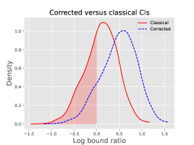
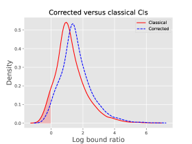
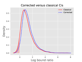
(a) $\alpha_{1}=4.0$	(b) $\alpha_{1}=6.0$	(c) $\alpha_{1}=10.0$

Figure 4: Study of the bounds in Corollary 3(a). Experiments with sample size $n=256$ with weak instrument scaling depending on the instrument strength $\alpha\in\{4.0,6.0,10.0\}$ in panels (a), (b) and (c), respectively. Density estimates of the log ratio between the classical CI estimate and the empirical IV error (red solid line) and the corrected CIs and the empirical IV error (blue dashed line).

With sample size $n=256$ and noise parameters $(\eta,\nu)=(1,0)$, we generated IV problems with weak instruments using the procedure described in equation (28). We considered three different instrument strengths—namely, $\alpha=\alpha_{1}/\sqrt{n}$ for $\alpha_{1}\in\{4.0,6.0,10.0\}$. For each setting of the parameters, we performed $M=10,000$ Monte Carlo trials, computing the log ratio of either the classical CI to the true IV error, or the corrected CI from equation (27a) to the true IV error. The classical CIs exhibited under coverage for instrument strengths $\alpha\in\{4.0,6.0\}$, with actual estimated coverages at $92\%$ and $93\%$, respectively. We computed the corrected CIs only when they were applicable according to the criteria (27a); the bounds were applicable in 19%, 87% and 100% of trials for the settings $\alpha_{1}\in\{4.0,6.0,10.0\}$, respectively.

Figure 4 shows density plots of these log ratios (with densities estimated using a standard Gaussian KDE). The classical CI ratios are plotted in red solid lines, with the corrected ones plotted in blue dashed lines; the shaded red area corresponds to the fraction of Monte Carlo trials for which the classical CIs were violated when the bound applied.

Corrected CIs for large $\kappa_{n}$:

Part (b) of Corollary 3 shows that the classical CIs can be overly large in problems for which the coefficient $\kappa_{n}$ is quite large, so that the condition $\kappa_{n}r_{1-\delta}>1$ applies. (With our setting $\delta=0.05$, we have $r_{1-\delta}=0.06$, so that we need $\kappa_{n}\gg 1$.) From the definition (26) of $\kappa_{n}$, it can be seen that large values of $\kappa_{n}$ are not likely to occur when the pairs $(Z,X)$ are independent and identically distributed. However, recall that our theory imposes only distributional assumptions on the sequence $\{Z_{i}\varepsilon_{i}\}_{i=1}^{n}$. There are no distributional assumptions on the covariates $\{X_{i}\}_{i=1}^{n}$, and this freedom can be exploited so as to construct ensembles for which $\kappa_{n}$ is large with high probability.

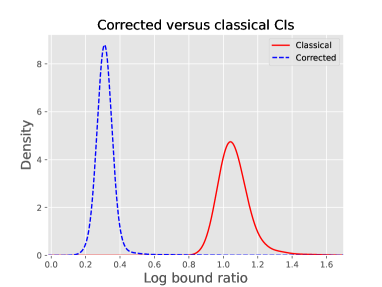
(a)	(b)

Figure 5: Density estimates of the log ratio between the classical CI estimate and the empirical IV error (red solid line) and the $\kappa_{n}$-corrected CIs and the empirical IV error (blue dashed line), computed over $M=10000$ trials. (a) Instrument strength $\alpha_{1}=0.25$. (b) Instrument strength $\alpha_{1}=0.75$.

In particular, suppose that we generate covariates $X$ from the ensemble (14) with endogeneity $\eta=0.10$ and additional noise level $\nu=10.0$, where the additional noise vector $W$ is constructed as follows:

$$W_{i}=Z_{i}G_{i}\qquad\mbox{for $i=1,\ldots,n$}$$

where $G\in{}^{n}$ is a zero-mean Gaussian random vector such that $\sum_{i=1}^{n}G_{i}=0$ with probability one. Since $Z_{i}\in\{-1,+1\}$, this construction ensures that $\sum_{i=1}^{n}Z_{i}W_{i}=\sum_{i=1}^{n}G_{i}=0$, so that the addition of $W$ to $X$ has no effect on $\sum_{i=1}^{n}Z_{i}X_{i}$. On the other hand, adding $W$ does affect the numerator $\sum_{i<j}(Z_{i}X_{i}-Z_{j}X_{j})^{2}$ in the definition of $\kappa_{n}$, in particular making it larger.

We conducted experiments using this ensemble with sample size $n$, and two settings of the instrument strength $\alpha=\alpha_{1}/\sqrt{n}$—namely, $\alpha_{1}\in\{0.25,0.75\}$. As before, we plotted the log ratio between the CI limits, either the classical one or the corrected using part (b) of Corollary 3. Figure 5 shows density estimates of these log ratios based on $M=10,000$ trials. respectively. With the weaker instrument $\alpha_{1}=0.25$ shown in panel (a), the inverse of the correction factor $\frac{r_{1-\delta}}{\kappa_{n}r_{1-\delta}-1}$ can be quite large, often around a factor of $10$ (or $1$ on the log scale). This effect dissipates for the somewhat stronger instrument level $\alpha_{1}=0.75$ shown in panel (b), and for very strong instruments, it is highly unlikely for $\kappa_{n}$ to be particularly large.

4.2 IV study of PM2.5 exposure

The conclusions drawn from this section are based on an original dataset compiled by the authors. The data is organized into census tracts, i.e. each census tract counts as a particular observation within our dataset. The motivating factor to consider data at a community level, as opposed to a individual level (the standard approach in similar studies), is due to the various publicly accessible datasets that provide community-level measurements. We are interested in estimating the effect of PM_2.5 exposure on various health metrics of the community. The response $y$ is taken from the PLACES project [18] which consists of prevalence rates of various negative health conditions including arthritis, asthma, blood pressure, cancer, heart disease, and stroke. measured between 2019-2020. We report our estimates of the effect of pollution for a variety of these health conditions. Here, the endogenous covariate of interest $X$ is the average daily PM_2.5 levels for each tract measured over the course of 2016, taken from the Public Health Tracking Network [17]. The exogeneous covariates $W$ include various other measurement for the census tract, such as race and demographics, educational attainment, employment by sector, median income, poverty rates, health insurance rates, indicators for states, and more, collected primarily from the 2020 US Census [31]. Our data set is summarized in Table 2. We provide a visualization of the average PM_2.5levels in the continental United States in 2016 at the resolution of individual counties in Figure 6.

Table 1: Summary statistics by census tracts

	Average	SD	USA (2020)
Population	4002	1629
Median household income	$ 68,600	$34,600	$74.580
Male	49%	5%	50%
Non-white	30%	26%	28%
Under 18	22%	7%	22%
Over 67	15%	8%	17%
Poverty rate	14%	11%	11%
Associates degree or higher	39%	19%	35%
Uninsurance rate	9%	7%	11%

(a) Our dataset consists of 58,761 census tracts treated as individual units. The first two reflects the average and standard deviation of each of the measurements indicated above across all the census tracts. The third column represents the actual average across the United States, to indicate that our data is a representative sample of the United States. Since the US Census data is often reported as number of people within a census tract that falls into a specific group, we have decided to use the fraction/percentage to standardize the tracts.

Table 2: Instrumental variable estimate of effects of pollution on negative health outcomes incidence rates and their standard errors.

	OLS	IV
Arthritis	-1.9	12.2
	(0.0)	(1.3)
Asthma	-0.5	5.2
	(0.0)	(0.5)
Cancer	0.0	1.3
	(0.0)	(0.3)
Heart disease	-0.2	2.9
	(0.0)	(0.4)
High blood pressure	-0.8	1.7
	(0.1)	(1.8)
Poor mental health	-0.2	5.6
	(0.0)	(0.7)
Poor sleep	0.5	0.1
	(0.1)	(1.2)
Stroke	-0.1	1.5
	(0.0)	(0.2)

(a) Results are reported in % increase per 10 PM_2.5

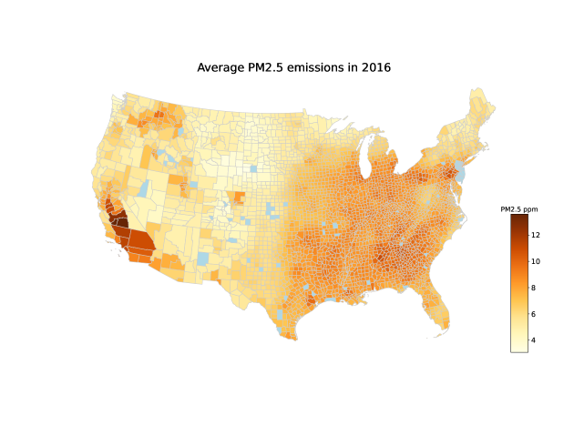
Figure 6: Average PM_2.5 levels in the continental USA in 2016; the darker the color the higher the fraction. Light blue indicates missing data for those specific counties.

The instrument $Z$ is a measure of the exposure of a given census tract to pollution caused by wildfires. Abstractly, our instrument is a gauge of a community’s susceptibility to wildfire smoke. We argue that this satisfies the exclusion restriction: proximity to wildfires has well-documented effects on the day-to-day pollution a specific community experiences, but is independent of other causes of negative health outcomes. An individuals exposure to wildfire pollution is dictated by geography and climate which, in the modern era, has little effect on one’s living and health conditions (especially the ones of interest). Thus it serves as a natural experiment by which we can analyze the effects of pollution on health outcomes. To describe our specific instrument, let $\mathcal{D}$ denote a dataset consisting of all the wildfires in 2016 that burned for at least 100 acres, as reported in the data given by the National Interagency Fire Center [13]. We define our instrument as

$$Z_{i}=\mathbf{1}\{Z_{i}^{*}\geq c\},\qquad\text{where}\qquad Z^{*}_{i}=\frac{1}{|\mathcal{D}|}\sum_{f\in\mathcal{D}}\frac{f_{\text{size}}}{(f_{\text{distance to $i$}})^{2}},$$ (29)

i.e. for every census tract $i$, we average across all the wildfires $f\in\mathcal{D}$ in 2016 the ratio of the size of the fire over the squared distance of the tract to the fire. Our final instrument then is a truncated version of the above instrument, $Z_{i}=\mathbf{1}\{Z_{i}^{*}\geq c\}$ for some constant $c$ chosen such that a reasonable fraction of the total instruments are both $0$ and $1$. Figure 7 depicts the fraction of census tracts within each county such that the wildfire smoke index was high, i.e. $Z_{i}=1$. With this instrument, our first stage $F$-statistic is $256$, so our instrument is strong. In the appendix, we report robustness checks using different thresholds and formulas and most of the results remain consistent with those reported below.

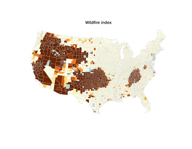
Figure 7: Fraction of census tracts within each county such that $Z_{i}=1$; the darker the color the higher the fraction. Light blue indicates missing data for those specific counties.

Our results are presented in Table 2. The standard errors are robust standard errors, i.e. computed via the standard errors as proved in Corollary 3. We remark that because our units are geographic in nature, the standard errors may be inaccurate due to spatial correlations that violate the independence assumption required by our estimator. The reported numbers are measured in % per 10 PM_2.5, i.e. the increase in incidence rates due to an increase in PM_2.5 concentration by 10. For reference, we also included the results of running OLS on the same dataset. Note that in every instance, OLS returns negative effect, indicating that an increase in pollution decreases the rates of these negative health outcomes. The instrumental variables regression indicates that PM_2.5 pollution ‘causes’ increases in the prevalence of these health conditions. For example, an increase in an average PM_2.5 level of $10$ in a given community results in a 3.3% increase in heart disease rates. Much of these results confirm existing association studies in the medical literature, i.e. the relationship between pollution and arthritis [8], asthma [43], cancer [41], heart disease [29], and stroke [38]. We remark that we also included the estimates of the effects of PM_2.5 on high blood pressure and poor sleep to indicate that our choice of instrument does not return significant effects for every possible response.

5 Discussion

In this paper, we presented a non-asymptotic analysis of the classical linear instrumental variable estimator in the $\ell_{2}$-norm. Additionally, we established guarantees for estimating the parameter of interest in the presence of exogeneous covariates. To the best of our knowledge, these are the first instances of such guarantees. We also establish, in the one-dimensional setting, confidence intervals for the IV estimate, as well as a novel measure for the strength of an instrument. In the strong-instrument setting our confidence intervals matches the classical asymptotic ones up to higher-order terms, but our measure of strength can be used to appropriately adjust the asymptotic ones to account for potentially weak instruments. Additionally, if the instrument is very weak our guarantees can be used to substantially sharpen the asymptotic confidence intervals. Furthermore, we applied our results to analyze the effect of air pollution on various negative health outcomes, using wildfire exposure as an instrument. Our IV estimates indicates that increased exposure to PM_2.5 pollution can increase ones risk of various health conditions such as arthritis, asthma, cancer, heart disease, poor mental health, and strokes.

Our results still leave open avenues of further investigation. The non-asymptotic confidence intervals we have derived still tend to be quite conservative or have stringent conditions that need to be met in order to be used. To make them truly usable in practice there are substantial improvements that would need to be made. Additionally, we have not addressed the question of confidence intervals in the presence of exogeneous covariates, which is the default setting in practice. In this paper we also only focused on the just-identified setting; when the number of instruments matches the number of covariates. Often times in practice we may have more instruments than we do covariates, known as the over-identified setting. Finally, instrumental variables are a special case of a broad class of estimators known as generalized method of moments (GMMs). Establishing non-asymptotic results for any of these more general settings is an interesting direction for future work.

Appendix A Proof of Theorems 1 and 2

In this appendix, we prove our two theorems that provide non-asymptotic bounds on the IV estimate itself (Theorem 1) and linear mappings thereof (Theorem 2). As noted following the statement of Theorem 2, it is actually more general than Theorem 1, so that it suffices to prove it.

A.1 Main argument

Introduce the shorthand $W_{n}\coloneq\frac{1}{n}\sum_{i=1}^{n}Z_{i}\varepsilon_{i}$. Using the form of the standard IV estimate, we can write

$$\widehat{\beta}-\beta^{*} =\widehat{\mathbf{\Gamma}}_{n}^{-1}W_{n}\;=\;\mathbf{\Gamma}_{n}^{-1}W_{n}+\Big{(}\widehat{\mathbf{\Gamma}}_{n}^{-1}\mathbf{\Gamma}_{n}-\mathbf{I}_{d}\Big{)}\mathbf{\Gamma}_{n}^{-1}W_{n}.$$

Applying $\mathbf{U}^{T}\in{}^{k\times d}$ to both sides yields

$$\mathbf{U}^{T}(\widehat{\beta}-\beta^{*}) =\;\mathbf{U}^{T}\mathbf{\Gamma}_{n}^{-1}W_{n}+\Big{[}\mathbf{U}^{T}\big{(}\widehat{\mathbf{\Gamma}}_{n}^{-1}\mathbf{\Gamma}_{n}-\mathbf{I}_{d}\big{)}\Big{]}\mathbf{\Gamma}_{n}^{-1}W_{n}.$$

Consequently, by the triangle inequality, we have

$$\|\mathbf{U}^{T}(\widehat{\beta}-\beta^{*})\|_{2} \leq\underbrace{\Big{\|}\frac{1}{n}\sum_{i=1}^{n}\mathbf{U}^{T}\mathbf{\Gamma}_{n}^{-1}Z_{i}\varepsilon_{i}\Big{\|}_{2}}_{T_{1}}+\gamma_{n}(\mathbf{\Gamma}_{n};\mathbf{U})\>\;\underbrace{\Big{\|}\frac{1}{n}\sum_{i=1}^{n}\mathbf{\Gamma}_{n}^{-1}Z_{i}\varepsilon_{i}\Big{\|}_{2}}_{T_{2}}$$ (30)

where $\gamma_{n}(\mathbf{\Gamma}_{n};\mathbf{U})\coloneq|\!|\!|\mathbf{U}^{T}(\widehat{\mathbf{\Gamma}}_{n}^{-1}\mathbf{\Gamma}_{n}-\mathbf{I}_{d})|\!|\!|_{{2}}$.

From this decomposition, we see that the central problem is controlling the Euclidean norms of two sums of random variables. In order to do so, we make use of the following auxiliary result:

Lemma 1.

Let $\{V_{i}\}_{i=1}^{n}$ be an independent sequence of zero-mean random vectors such that $\big{\|}V_{i}\big{\|}_{2}\leq b$ almost surely. Then for any $\delta\in(0,1)$, we have

$$\big{\|}\sum_{i=1}^{n}V_{i}\big{\|}_{2}\leq\mathbb{E}\left[\big{\|}\sum_{i=1}^{n}V_{i}\big{\|}_{2}\right]+\sqrt{2\log(\tfrac{1}{\delta})\mathbb{E}|\!|\!|\sum_{i=1}^{n}V_{i}V_{i}^{T}|\!|\!|_{{2}}}+3b\log(\tfrac{1}{\delta})$$ (31)

with probability at least $1-\delta$.

See Section A.2 for the proof.

We use this lemma to bound each of the two terms on the RHS of equation (30).

Bounding the quantity $T_{1}$:

We first apply Lemma 1 with $V_{i}\coloneq\mathbf{U}^{T}\mathbf{\Gamma}_{n}^{-1}(\varepsilon_{i}Z_{i})$ in order to bound the first term $T_{1}$. From our set-up, each $V_{i}$ is zero-mean and satisfies the $b$-boundedness condition; moreover, the sequence is independent by assumption. Recalling the vector $G_{n}$ from equation (10), we have $\sum_{i=1}^{n}V_{i}=\sqrt{n}\mathbf{U}^{T}G_{n}$. As for the term $|\!|\!|\sum_{i=1}^{n}V_{i}V_{i}^{T}|\!|\!|_{{2}}$, we have

$$\sum_{i=1}^{n}V_{i}V_{i}^{T} =\mathbf{U}^{T}\mathbf{\Gamma}_{n}^{-1}\Big{(}\frac{1}{n}\sum_{i=1}^{n}\varepsilon_{i}^{2}Z_{i}Z_{i}^{T}\Big{)}\mathbf{\Gamma}_{n}^{-T}\mathbf{U}\;=\;n\mathbf{U}^{T}\mathbf{\Gamma}_{n}^{-1}\widetilde{\mathbf{\Sigma}}_{n}\mathbf{\Gamma}_{n}^{-T}\mathbf{U},$$

where the final equality uses the definition of $\widetilde{\mathbf{\Sigma}}_{n}$ from equation (9b). Dividing by $n$ and putting together the pieces, we have shown that

$$\Big{\|}\frac{1}{n}\sum_{i=1}^{n}\mathbf{U}^{T}\mathbf{\Gamma}_{n}^{-1}Z_{i}\varepsilon_{i}\Big{\|}_{2} \leq\frac{\mathbb{E}\|\mathbf{U}^{T}G_{n}\|_{2}}{\sqrt{n}}+\frac{1}{\sqrt{n}}\sqrt{2\log(\tfrac{1}{\delta})\mathbb{E}|\!|\!|\mathbf{U}^{T}\widehat{\mathbf{\Gamma}}_{n}^{-1}\widetilde{\mathbf{\Sigma}}_{n}\widehat{\mathbf{\Gamma}}_{n}^{-T}\mathbf{U}|\!|\!|_{{2}}}+\frac{3b\log(\tfrac{1}{\delta})}{n}.$$ (32a)

Bounding the quantity $T_{2}$:

The previous argument applies to a general $\mathbf{U}$ so that we can apply it with $\mathbf{U}=\mathbf{I}_{d}$. (Our assumptions imply that the random vectors $\mathbf{\Gamma}_{n}^{-1}Z_{i}\varepsilon_{i}$ are also $b$-bounded.) Consequently, by recourse to the bound (32a), we can conclude that

$$T_{2} \leq\frac{\mathbb{E}\|G_{n}\|_{2}}{\sqrt{n}}+\frac{1}{\sqrt{n}}\sqrt{2\log(\tfrac{1}{\delta})\mathbb{E}|\!|\!|\widehat{\mathbf{\Gamma}}_{n}^{-1}\widetilde{\mathbf{\Sigma}}_{n}\widehat{\mathbf{\Gamma}}_{n}^{-T}|\!|\!|_{{2}}}+\frac{3b\log(\tfrac{1}{\delta})}{n}.$$ (32b)

Finally, combining the two bounds (32a) and (32b) with our initial decomposition (30) yields the claim of Theorem 2.

A.2 Proof of Lemma 1

We control $\big{\|}\sum_{i=1}^{n}V_{i}\big{\|}_{2}$ by representing it as the supremum of an empirical process. Note that we can write

$$\big{\|}\sum_{i=1}^{n}V_{i}\big{\|}_{2}=\sup_{\|u\|_{2}=1}\sum_{i=1}^{n}\langle u,\,V_{i}\rangle=\sup_{f_{u}\in\mathpzc{F}}\sum_{i=1}^{n}f_{u}(V_{i}),$$

where we define $\mathpzc{F}=\{f_{u}:f_{u}(x)=\langle u,x\rangle,\,u\in\mathbb{S}^{d-1}\}$, i.e. $\mathpzc{F}$ is the set of linear functions with unit norm coefficient vectors. With this set-up, we perform the necessary calculations in order to apply a result due to Klein and Rio (see Theorem 5 in Section C.1).

For all $f_{u}\in\mathpzc{F}$, we have

$$\mathbb{E}[f_{u}(V_{i})]=0,\quad\text{and}\quad\|f_{u}\|_{\infty}=\sup_{z}|f_{u}(V)|=|\langle u,V\rangle|\leq b\quad a.s.,$$

where we have used the assumption that the vectors $V=\varepsilon\mathbf{\Gamma}_{n}^{-1}Z$ are $b$-uniformly bounded.

Additionally, we have

$$\nu\coloneq\mathbb{E}\left[\sup_{f_{u}\in\mathpzc{F}}\sum_{i=1}^{n}f^{2}(V_{i})\right]=\mathbb{E}\left[\sup_{\|u\|_{2}=1}\,u^{T}\big{(}\sum_{i=1}^{n}V_{i}V_{i}^{T}\big{)}u\right] =\mathbb{E}|\!|\!|\sum_{i=1}^{n}V_{i}V_{i}^{T}|\!|\!|_{{2}}$$

$$=\mathbb{E}\Big{|}\!\Big{|}\!\Big{|}\mathbf{\Gamma}_{n}^{-1}\widetilde{\mathbf{\Sigma}}_{n}\mathbf{\Gamma}_{n}^{-T}\Big{|}\!\Big{|}\!\Big{|}_{{2}},$$

where the final equality uses the definition of $V_{i}$ and $\widetilde{\mathbf{\Sigma}}_{n}$. With these calculations in place, applying Theorem 5 from Section C.1 yields

$$\big{\|}\frac{1}{n}\sum_{i=1}^{n}V_{i}\big{\|}_{2}\leq\mathbb{E}\big{\|}\frac{1}{n}\sum_{i=1}^{n}V_{i}\big{\|}_{2}+\frac{1}{\sqrt{n}}\sqrt{2\log(\tfrac{1}{\delta})\mathbb{E}\big{\|}\mathbf{\Gamma}_{n}^{-1}\widetilde{\mathbf{\Sigma}}_{n}\mathbf{\Gamma}_{n}^{-T}\big{\|}_{2}}+\frac{3b\log(\tfrac{1}{\delta})}{n},$$

with probability at least $1-\delta$.

A.3 Extensions to unbounded random variables

In our current statements of Theorems 1 and 2, we impose $b$-boundedness conditions on the random vectors $\mathbf{\Gamma}_{n}^{-1}Z_{i}\varepsilon_{i}$. These conditions allow us to apply a concentration inequality for empirical processes due to Bousquet with sharp constants. However, the underlying proof technique is not restricted to bounded random vectors; by leveraging results on unbounded empirical processes, we can obtain generalizations of Theorems 1 and 2. For example, Adamczak [1] provides bounds on the suprema of empirical processes under Orlicz norm conditions. One can also make use of truncation arguments to handle this more general setting.

Appendix B Proof for confidence interval guarantees

In this section, we provide the proofs of our two main results on confidence intervals—namely,  Theorem 3 and Corollary 3.

B.1 Proof of Theorem 3

Let $V\sim\mathcal{N}(0,1)$ be standard normal. By the Berry–Esseen theorem (c.f. Theorem 6), for any $r>0$, we have

$$\left|\mathbb{P}\left[\sqrt{n}\big{|}u^{T}\widehat{\mathbf{\Gamma}}_{n}\widehat{\Delta}\big{|}\geq r\sqrt{u^{T}\mathbf{\Sigma}_{n}u}\right]-\mathbb{P}\big{[}|V|\geq r\big{]}\right|\leq\frac{cm_{3}}{\sqrt{n}}.$$ (33)

The choice $r=r_{\delta}$ ensures that $\mathbb{P}[|V|\geq r_{\delta}]=\delta$, whence

$$\sqrt{n}\big{|}u^{T}\widehat{\mathbf{\Gamma}}_{n}\widehat{\Delta}\big{|}\leq r_{\delta}\sqrt{u^{T}\mathbf{\Sigma}_{n}u}$$ (34a)

with probability at least $$1-\delta-\frac{cm_{3}}{\sqrt{n}}$$.

Introduce the shorthand $W_{i}\coloneq\langle u,\,Z_{i}\rangle$, and observe that $\sqrt{u^{T}\mathbf{\Sigma}_{n}u}=\sqrt{\frac{1}{n}\sum_{i=1}^{n}\mathbb{E}[\varepsilon_{i}^{2}W_{i}^{2}]}$. Using the $b$-boundedness and independence condition, we can apply Theorem 10 in the paper [30] so as to guarantee that

$$\sqrt{u^{T}\mathbf{\Sigma}_{n}u} \leq\sqrt{\frac{1}{n(n-1)}\sum_{i<j}(\varepsilon_{i}W_{i}-\varepsilon_{j}W_{j})^{2}}+b\sqrt{\frac{8\log(1/\delta^{\prime})}{n-1}}.$$ (34b)

with probability at least $1-\delta^{\prime}$.

Recall the definition (22) of $e_{n}(\widehat{\Delta})$, as well as the matrix $\widehat{\mathbf{\Sigma}}_{n}$ from equation (21a). We claim that the proof will be complete if we can show that

$$\sqrt{\frac{1}{n(n-1)}\sum_{i<j}(\varepsilon_{i}W_{i}-\varepsilon_{j}W_{j})^{2}} \leq\sqrt{u^{T}\widehat{\mathbf{\Sigma}}_{n}u}+e_{n}(\widehat{\Delta})$$ (34c)

Indeed, if this bound holds, then combining it with inequalities (34a) and (34b) yields

$$\sqrt{n}\big{|}u^{T}\widehat{\mathbf{\Gamma}}_{n}\widehat{\Delta}\big{|}\leq r_{\delta}\Big{\{}\sqrt{u^{T}\widehat{\mathbf{\Sigma}}_{n}u}+b\sqrt{\frac{8\log(1/\delta^{\prime})}{n-1}}+e_{n}(\widehat{\Delta})\Big{\}}$$ (35)

with probability at least $1-\delta-\delta^{\prime}-\frac{cm_{3}}{\sqrt{n}}$, which establishes the bound (23) from Theorem 3.

Proof of the bound (34c):

We begin by observing the decomposition

$$\underbrace{\varepsilon_{i}W_{i}-\varepsilon_{j}W_{j}}_{a_{ij}} \quad=\quad\underbrace{\widehat{\varepsilon}_{i}W_{i}-\widehat{\varepsilon}_{j}W_{j}}_{b_{ij}}\quad+\quad\underbrace{\langle X_{i},\,\widehat{\Delta}\rangle W_{i}-\langle X_{j},\,\widehat{\Delta}\rangle W_{j}}_{c_{ij}}.$$ (36)

Since $\|a\|_{2}\leq\|b\|_{2}+\|c\|_{2}$ by the triangle inequality, we have

$$\underbrace{\sqrt{\sum_{i<j}(\varepsilon_{i}W_{i}-\varepsilon_{j}W_{j})^{2}}}_{\|a\|_{2}} \leq\underbrace{\sqrt{\sum_{i<j}\left(\widehat{\varepsilon}_{i}W_{i}-\widehat{\varepsilon}_{j}W_{j}\right)^{2}}}_{\|b\|_{2}}+\underbrace{\sqrt{\sum_{i<j}\left(\langle X_{i},\,\widehat{\Delta}\rangle W_{i}-\langle X_{j},\,\widehat{\Delta}\rangle W_{j}\right)^{2}}}_{\|c\|_{2}}.$$

Dividing both sides by $\sqrt{n(n-1)}$ and recalling the definition (22) of $e_{n}(\widehat{\Delta})$, we have shown that

$$\sqrt{\frac{1}{n(n-1)}\sum_{i<j}(\varepsilon_{i}W_{i}-\varepsilon_{j}W_{j})^{2}} \leq\sqrt{\frac{1}{n(n-1)}\sum_{i<j}\left(\widehat{\varepsilon}_{i}W_{i}-\widehat{\varepsilon}_{j}W_{j}\right)^{2}}+e_{n}(\widehat{\Delta})$$

By Lemma 2(a), we have the equivalence

$$\frac{1}{n(n-1)}\sum_{i<j}\left(\widehat{\varepsilon}_{i}W_{i}-\widehat{\varepsilon}_{j}W_{j}\right)^{2} =\frac{1}{n-1}\sum_{i=1}^{n}\big{(}\widehat{\varepsilon}_{i}W_{i}-\frac{1}{n}\sum_{j=1}^{n}\widehat{\varepsilon}_{j}W_{j}\big{)}^{2}$$

But recalling that $W_{i}=\langle u,\,Z_{i}\rangle$, we have

$$\sum_{j=1}^{n}\widehat{\varepsilon}_{j}W_{j}\;=\;\langle u,\,\sum_{j=1}^{n}\big{(}y_{i}-\langle X_{i},\,\widehat{\beta}\rangle\big{)}Z_{j}\rangle \stackrel{{\scriptstyle(\star)}}{{=}}0,$$

where equality $(\star)$ follows from the optimality conditions that define the IV estimate. Thus, we have shown that

$$\frac{1}{n(n-1)}\sum_{i<j}\left(\widehat{\varepsilon}_{i}W_{i}-\widehat{\varepsilon}_{j}W_{j}\right)^{2} =\frac{1}{n-1}\sum_{i=1}^{n}\widehat{\varepsilon}^{2}_{i}W_{i}^{2}\;=\;u^{T}\widehat{\mathbf{\Sigma}}_{n}u,$$

thereby proving the claim (34c).

B.2 Proof of Corollary 1

We begin by applying Theorem 3 with the vector $v=\mathbf{\Gamma}_{n}^{-1}u$, from which we are guaranteed to have

$$\sqrt{n}|\langle u,\,\mathbf{\Gamma}_{n}^{-1}\widehat{\mathbf{\Gamma}}_{n}\widehat{\Delta}\rangle| \leq r_{\delta}\left\{\sqrt{u^{T}\mathbf{\Gamma}_{n}^{-1}\widehat{\mathbf{\Sigma}}_{n}\mathbf{\Gamma}_{n}^{-T}u}+b\|\mathbf{\Gamma}_{n}^{-T}u\|_{2}\sqrt{\frac{8\log(1/\delta^{\prime})}{n-1}}+e_{n}(\widehat{\Delta})\right\}.$$ (37a)

with the claimed probability. An application of the triangle inequality ensures that

$$\sqrt{n}|\langle u,\,\widehat{\Delta}\rangle| \leq\sqrt{n}|\langle u,\,\mathbf{\Gamma}_{n}^{-1}\widehat{\mathbf{\Gamma}}_{n}\widehat{\Delta}\rangle|+\sqrt{n}|\langle u,\,(\mathbf{\Gamma}_{n}^{-1}\widehat{\mathbf{\Gamma}}_{n}-\mathbf{I}_{d})\widehat{\Delta}\rangle|$$

$$=\sqrt{n}|\langle u,\,\mathbf{\Gamma}_{n}^{-1}\widehat{\mathbf{\Gamma}}_{n}\widehat{\Delta}\rangle|+\sqrt{n}\big{|}u^{T}\mathbf{D}_{n}\widehat{\Delta}\big{|}.$$ (37b)

Similarly, we have

$$\sqrt{u^{T}\mathbf{\Gamma}_{n}^{-1}\widehat{\mathbf{\Sigma}}_{n}\mathbf{\Gamma}_{n}^{-T}u}\>=\>\|\widehat{\mathbf{\Sigma}}_{n}^{1/2}\mathbf{\Gamma}_{n}^{-T}u\|_{2} \leq\|\widehat{\mathbf{\Sigma}}_{n}^{1/2}\widehat{\mathbf{\Gamma}}_{n}^{-T}u\|_{2}+\|\widehat{\mathbf{\Sigma}}_{n}^{1/2}\big{(}\mathbf{\Gamma}_{n}^{-T}-\widehat{\mathbf{\Gamma}}_{n}^{-T}\big{)}u\|_{2}$$

$$=\sqrt{u^{T}\widehat{\mathbf{\Gamma}}_{n}^{-1}\widehat{\mathbf{\Sigma}}_{n}\widehat{\mathbf{\Gamma}}_{n}^{-T}u}+\|\widehat{\mathbf{\Sigma}}_{n}^{1/2}\widehat{\mathbf{\Gamma}}_{n}^{-T}\mathbf{D}_{n}^{T}u\|_{2}.$$ (37c)

Combining the bounds (37b) and (37c) with our original inequality (37a) yields

$$\sqrt{n}|\langle u,\,\mathbf{\Gamma}_{n}^{-1}\widehat{\mathbf{\Gamma}}_{n}\widehat{\Delta}\rangle| \leq r_{\delta}\left\{\sqrt{u^{T}\widehat{\mathbf{\Gamma}}_{n}^{-1}\widehat{\mathbf{\Sigma}}_{n}\widehat{\mathbf{\Gamma}}_{n}^{-T}u}+b\|\mathbf{\Gamma}_{n}^{-T}u\|_{2}\sqrt{\frac{8\log(1/\delta^{\prime})}{n-1}}\right\}+r_{\delta}e_{n}(\widehat{\Delta})+\widetilde{e}_{n}(\widehat{\Delta},\mathbf{D}_{n}),$$

where

$$\widetilde{e}_{n}(\widehat{\Delta},\mathbf{D}_{n}) \coloneq\underbrace{r_{\delta}\|\widehat{\mathbf{\Sigma}}_{n}^{1/2}\widehat{\mathbf{\Gamma}}_{n}^{-T}\mathbf{D}_{n}^{T}u\|_{2}+b\;\|\widehat{\mathbf{\Gamma}}_{n}^{T}\mathbf{D}_{n}^{T}u\|_{2}\;\sqrt{\tfrac{8\log(1/\delta^{\prime})}{n-1}}}_{T_{4}}+\underbrace{\sqrt{n}|u^{T}\mathbf{D}_{n}\widehat{\Delta}|}_{T_{5}}.$$

As noted previously, we have $e_{n}(\widehat{\Delta})\leq|\!|\!|\mathbf{Q}_{n}(v)|\!|\!|_{{2}}\|\widehat{\Delta}\|_{2}$, and moreover, we see that

$$T_{4} \leq|\!|\!|\mathbf{D}_{n}|\!|\!|_{{2}}\left\{r_{\delta}|\!|\!|\widehat{\mathbf{\Gamma}}_{n}^{-1}\widetilde{\mathbf{\Sigma}}_{n}^{1/2}|\!|\!|_{{2}}+b|\!|\!|\widehat{\mathbf{\Gamma}}_{n}|\!|\!|_{{2}}\sqrt{\tfrac{8\log(1/\delta^{\prime})}{n-1}}\right\}\quad\mbox{and}\quad T_{5}\leq\sqrt{n}|\!|\!|\mathbf{D}_{n}|\!|\!|_{{2}}\|\widehat{\Delta}\|_{2}.$$

Putting together the pieces completes the proof.

B.3 Proof of Corollary 2

The main idea is to control the error over the $\ell_{1}$-ball centered at $\mathbf{\Gamma}_{n}^{-1}u$, and instead of uniformly controlling over some $\epsilon$-net, we can uniformly control over the vertices of the $\ell_{1}$-ball due to the fact that the optimal solution of a linear program is at the extremal points.

For convenience, we use $\mathbb{B}_{1}(v;\lambda)$ to denote the $\ell_{1}$ ball around $v$ with radius $\lambda$, i.e.

$$\mathbb{B}_{1}(v;\lambda)=\{w\in\mathbb{R}^{d}\,:\,\|w-v\|_{1}\leq\lambda\}=\text{conv}\left\{w\pm\lambda e_{i}\,:\,i\in[d]\right\}.$$

We have that $\widehat{\mathbf{\Gamma}}_{n}^{-1}u\in\mathbb{B}_{1}(v;\lambda)$ and thus

$$\sqrt{n}\,|\langle u,\widehat{\Delta}\rangle| =\sqrt{n}\,|\langle\widehat{\mathbf{\Gamma}}_{n}^{-1}u,\widehat{\mathbf{\Gamma}}_{n}\widehat{\Delta}\rangle|$$

$$\stackrel{{\scriptstyle(a)}}{{\leq}}\sqrt{n}\,\sup_{w\in\mathbb{B}_{1}(\mathbf{\Gamma}_{n}^{-1}u;\lambda)}|\langle w,\widehat{\mathbf{\Gamma}}_{n}\widehat{\Delta}\rangle|$$

$$\stackrel{{\scriptstyle(b)}}{{=}}\sqrt{n}\cdot\max_{\begin{subarray}{c}v\in\{+\mathbf{\Gamma}_{n}^{-1}u,-\mathbf{\Gamma}_{n}^{-1}u\}\\ w\in E\end{subarray}}\,\langle u+\lambda w,\widehat{\mathbf{\Gamma}}_{n}\widehat{\Delta}\rangle$$

$$=\sqrt{n}\cdot\max_{w\in E}|\langle\mathbf{\Gamma}_{n}^{-1}u+\lambda w,\widehat{\mathbf{\Gamma}}_{n}\widehat{\Delta}\rangle|$$

Step (a) follows from above, and step (b) follows from the fact that the optimal solution for any linear program exists at one of the vertices.

By Berry-Esseen we have

$$\mathbb{P}\left(\sqrt{n}\cdot\max_{w\in E}|\langle\mathbf{\Gamma}_{n}^{-1}u+\lambda w,\widehat{\mathbf{\Gamma}}_{n}\widehat{\Delta}\rangle|\geq\epsilon\right)$$

$$\qquad\qquad\leq\mathbb{P}\left(\max_{w\in E}|\langle\mathbf{\Gamma}_{n}^{-1}u+\lambda w,\mathbf{\Sigma}_{n}^{1/2}V\rangle|\geq\epsilon\right)+\frac{cm_{3}}{\sqrt{n}}$$

where $V\sim\mathcal{N}(0,\mathbf{I}_{d})$. By a union bound we have

$$\mathbb{P}\left(\max_{w\in E}|\langle\mathbf{\Gamma}_{n}^{-1}u+\lambda w,\mathbf{\Sigma}_{n}^{1/2}V\rangle|\geq\epsilon\right) \leq\sum_{i=1}^{d}\mathbb{P}\left(|\langle\mathbf{\Gamma}_{n}^{-1}u+\lambda e_{i},\mathbf{\Sigma}_{n}^{1/2}V\rangle|\geq\epsilon\right)$$

$$\qquad\qquad+\sum_{i=1}^{d}\mathbb{P}\left(|\langle\mathbf{\Gamma}_{n}^{-1}u-\lambda e_{i},\mathbf{\Sigma}_{n}^{1/2}V\rangle|\geq\epsilon\right).$$

Using the shorthand

$$\sigma^{2}(e_{i})\coloneq(\mathbf{\Gamma}_{n}^{-1}u+\lambda e_{i})^{T}\mathbf{\Sigma}_{n}(\mathbf{\Gamma}_{n}^{-1}u+\lambda e_{i})$$

we have $\langle\mathbf{\Gamma}_{n}^{-1}u-\lambda e_{i},\mathbf{\Sigma}_{n}^{1/2}V\rangle\sim\mathcal{N}(0,\sigma^{2}(e_{i}))$, and that

$$\mathbb{P}\left(|\langle\mathbf{\Gamma}_{n}^{-1}u+\lambda e_{i},\mathbf{\Sigma}_{n}^{1/2}V\rangle|\geq\epsilon\right)=2-2\Phi\left(\frac{\epsilon}{\sigma(e_{i})}\right).$$

If we use $\epsilon=r_{\delta/2d}\sup_{w\in E}\sigma(w)$, we obtain

$$\max_{w\in E}|\langle\mathbf{\Gamma}_{n}^{-1}u+\lambda w,\mathbf{\Sigma}_{n}^{1/2}V\rangle|\leq r_{\delta/2d}\sup_{w\in E}\sigma(w)$$

with probability exceeding $1-\delta$.

We now focus on controlling the final term. We have that by applying Maurer and Pontil uniformly,

$$\sup_{w\in E}\sigma(w) \leq\sup_{w\in E}\underbrace{\sqrt{(\mathbf{\Gamma}_{n}^{-1}u+\lambda w)^{T}\widehat{\mathbf{\Sigma}}_{n}(\mathbf{\Gamma}_{n}^{-1}u+\lambda w)}}_{S_{1}}$$

$$\qquad\qquad+b\sqrt{\frac{8\log(2d/\delta^{\prime})}{n-1}}\cdot\sup_{w\in E}\|\mathbf{\Gamma}_{n}^{-1}u+\lambda w\|_{2}$$

$$\qquad\qquad+\sup_{w\in E}\underbrace{e_{n}(\widehat{\Delta};\mathbf{\Gamma}_{n}^{-1}u+\lambda w)}_{S_{2}}.$$

We analyze the terms individually; for $S_{1}$ we have

$$S_{1}=\|\mathbf{\Gamma}_{n}^{-1}u+\lambda w\|_{\widehat{\mathbf{\Sigma}}_{n}} \leq\|\widehat{\mathbf{\Gamma}}_{n}^{-1}u\|_{\widehat{\mathbf{\Sigma}}_{n}}+\|\mathbf{\Gamma}_{n}^{-1}u-\widehat{\mathbf{\Gamma}}_{n}^{-1}u\|_{\widehat{\mathbf{\Sigma}}_{n}}+\lambda\|w\|_{\widehat{\mathbf{\Sigma}}_{n}}$$

$$\leq\sqrt{u^{T}\widehat{\mathbf{\Gamma}}_{n}^{-T}\widehat{\mathbf{\Sigma}}_{n}\widehat{\mathbf{\Gamma}}_{n}^{-1}u}+2\lambda\cdot|||\widehat{\mathbf{\Sigma}}_{n}|||_{2}.$$

For $S_{2}$ we have

$$S_{2}\leq\|\widehat{\Delta}\|_{2}\cdot\sup_{w\in E}\sqrt{|||\mathbf{Q}_{n}(\mathbf{\Gamma}_{n}^{-1}u+\lambda w)|||_{2}}$$

Putting together the pieces, we conclude

$$\sqrt{n}|\langle u,\widehat{\Delta}\rangle| \leq r_{\delta/2d}\left\{\sqrt{u^{T}\widehat{\mathbf{\Gamma}}_{n}^{-T}\widehat{\mathbf{\Sigma}}_{n}\widehat{\mathbf{\Gamma}}_{n}^{-1}u}+b\cdot\sqrt{\frac{8\log(2d/\delta^{\prime})}{n-1}}\cdot\sup_{w\in E}\|\mathbf{\Gamma}_{n}^{-1}u+\lambda w\|_{2}\right.$$

$$\qquad\qquad\qquad\qquad\left.+2\lambda\cdot|\!|\!|\widehat{\mathbf{\Sigma}}_{n}|\!|\!|_{{2}}+\|\widehat{\Delta}\|_{2}\cdot\sup_{w\in E}\sqrt{|\!|\!|\mathbf{Q}_{n}(\mathbf{\Gamma}_{n}^{-1}u+\lambda w)|\!|\!|_{{2}}}\right\},$$

as desired.

B.4 Proof of Corollary 3

We now prove the corollary applicable to the univariate case ($d=1$), so that both $\widehat{\mathbf{\Gamma}}_{n}$ and $\widehat{\mathbf{\Sigma}}_{n}$ are scalar quantities, and $u=1$.

Proof of part (a):

Beginning with the definition (22) of $e_{n}(\widehat{\Delta})$, in the scalar case, it simplifies to

$$e_{n}(\widehat{\Delta}) =\frac{1}{\sqrt{n}}\frac{\sqrt{\frac{1}{n(n-1)}\sum_{i<j}\big{(}Z_{i}X_{i}-Z_{j}X_{j})^{2}}}{|\frac{1}{n}\sum_{i=1}^{n}Z_{i}X_{i}|}\;|\widehat{\Delta}|\;=\;\sqrt{n}\;\kappa_{n}|\widehat{\mathbf{\Gamma}}_{n}|\;|\widehat{\Delta}|,$$

where we recall the definition (26) of the scalar $\kappa_{n}$.

Substituting this relation into the bound (35) and re-arranging yields

$$\sqrt{n}|\widehat{\mathbf{\Gamma}}_{n}||\widehat{\Delta}|\;\big{\{}1-r_{\delta}\kappa_{n}\big{\}} \leq r_{\delta}\Big{\{}\sqrt{\widehat{\mathbf{\Sigma}}_{n}}+b\sqrt{\frac{8\log(1/\delta^{\prime})}{n-1}}\Big{\}}.$$

As long as $1-r_{\delta}\kappa_{n}>0$, we can rescale both sides by $(1-r_{\delta}\kappa_{n})\;|\widehat{\mathbf{\Gamma}}_{n}|$, which yields the claimed bound.

Proof of part (b):

Returning to our Berry–Esseen bound (33), we set $r=r_{1-\delta}$ to conclude that

$$\sqrt{n}|\widehat{\mathbf{\Gamma}}_{n}|\;|\widehat{\Delta}| \geq r_{1-\delta}\sqrt{\mathbf{\Sigma}_{n}}$$ (38a)

with probability at least $$1-\delta-\frac{cm_{3}}{\sqrt{n}} u=1 \widehat{\mathbf{\Gamma}}_{n} \mathbf{\Sigma}_{n}$$. (Here we recall that in the univariate case, and that both and are scalars.)

From Theorem 10 in the paper [30], we are guaranteed to have

$$\sqrt{\mathbf{\Sigma}_{n}} \geq\sqrt{\frac{1}{n(n-1)}\sum_{i<j}(\varepsilon_{i}W_{i}-\varepsilon_{j}W_{j})^{2}}-b\sqrt{\frac{8\log(1/\delta^{\prime})}{n-1}}$$ (38b)

with probability at least $1-\delta^{\prime}$, where in this scalar case $W_{i}=\langle u,\,Z_{i}\rangle=Z_{i}$.

Again using the decomposition (36), the triangle inequality implies that

$$\underbrace{\sqrt{\sum_{i<j}(\varepsilon_{i}W_{i}-\varepsilon_{j}W_{j})^{2}}}_{\|a\|_{2}} \geq\underbrace{\sqrt{\sum_{i<j}\left(\langle X_{i},\,\widehat{\Delta}\rangle W_{i}-\langle X_{j},\,\widehat{\Delta}\rangle W_{j}\right)^{2}}}_{\|c\|_{2}}-\underbrace{\sqrt{\sum_{i<j}\left(\widehat{\varepsilon}_{i}W_{i}-\widehat{\varepsilon}_{j}W_{j}\right)^{2}}}_{\|b\|_{2}}.$$ (38c)

Combining equations (38a),  (38b) and (38c), we have shown that

$$\sqrt{n}\>|\widehat{\mathbf{\Gamma}}_{n}|\>|\widehat{\Delta}| \geq r_{1-\delta}\Big{\{}\sqrt{n}\kappa_{n}|\widehat{\mathbf{\Gamma}}_{n}||\widehat{\Delta}|-\sqrt{\widehat{\mathbf{\Sigma}}_{n}}-b\sqrt{\frac{8\log(1/\delta^{\prime})}{n-1}}\Big{\}}.$$

Re-arranging terms yields

$$\sqrt{n}\>|\widehat{\mathbf{\Gamma}}_{n}|\>|\widehat{\Delta}|\big{\{}\kappa_{n}r_{1-\delta}-1\big{\}} \leq r_{1-\delta}\Big{\{}\sqrt{\widehat{\mathbf{\Sigma}}_{n}}+b\sqrt{\frac{8\log(1/\delta^{\prime})}{n-1}}\Big{\}}.$$

As long as $\kappa_{n}r_{1-\delta}>1$, we can divide both sides by $|\widehat{\mathbf{\Gamma}}_{n}|\big{(}\kappa_{n}r_{1-\delta}-1\big{)}$ to conclude the proof.

Appendix C Some auxiliary results

In this appendix, we collect the statements of various tail bounds, Berry–Esseen bounds, and sample variance bounds used in our analysis.

C.1 Tail and concentration inequalities

Portions of our analysis make use of Bernstein’s inequality:

Theorem 4.

Let $\{X_{i}\}_{i=1}^{n}$ be independent zero-mean random variables such that $|X_{i}|\leq b$ almost surely for each $i$. Then

$$\mathbb{P}\left(\sum_{i=1}^{n}X_{i}\geq t\right)\leq\exp\left(-\frac{\tfrac{1}{2}t^{2}}{\sum_{i=1}^{n}\mathbb{E}[X_{i}^{2}]+\tfrac{1}{3}bt}\right)\qquad\mbox{for each $t>0$.}$$ (39)

There are various extensions of Bernstein’s inequality to suprema of empirical processes. In particular, let $\mathpzc{F}$ be a countable class of functions $f:\mathcal{X}\to\mathbb{R}$, and let $\{X_{i}\}_{i=1}^{n}$ be a sequence of independent random variables in $\mathcal{X}$ such that $\mathbb{E}[f(X_{i})]=0$ for each $f\in\mathpzc{F}$. It is frequently of interest to control the tails of the random variable $Z_{n}\coloneq\sup_{f\in\mathpzc{F}}\sum_{i=1}^{n}f(X_{i})$. In order to do so, we make use of following result due to Klein and Rio [25]:

Theorem 5.

Suppose that $\sup_{f\in\mathpzc{F},i\in[n]}|f(X_{i})|\leq b$ almost surely. Then for all $t>0$, we have

$$\mathbb{P}[Z_{n}\geq\mathbb{E}[Z_{n}]+t]\leq\exp\left(-\frac{t^{2}}{2\nu^{2}+3bt}\right)$$ (40)

where $\nu^{2}\coloneq\mathbb{E}[\sup\limits_{f\in\mathpzc{F}}\sum_{i=1}^{n}f^{2}(X_{i})]$.

C.2 Berry–Esseen theorem

We also make use of some quantitative versions of the Berry–Esseen theorem.

Theorem 6 ([34]).

Let $\{X_{i}\}_{i=1}^{n}$ be a sequence of zero-mean independent random vectors in $\mathbb{R}^{d}$ such that $\sum_{i=1}^{n}\mathbb{E}[X_{i}X_{i}^{T}]=\mathbf{I}_{d}$, and define $W=\sum_{i=1}^{n}X_{i}$. Letting $V\sim\mathcal{N}(0,\mathbf{I}_{d})$ be standard normal, we have

$$\left|\mathbb{P}(W\in A)-\mathbb{P}(V\in A)\right|\leq\big{(}42d^{1/4}+16\big{)}\sum_{i=1}^{n}\mathbb{E}\|X_{i}\|_{2}^{3}.$$

valid for any measurable convex set $A\subset\mathbb{R}^{d}$.

In our analysis, it is convenient to make use of the following consequence of this theorem. Let $\{X_{i}\}_{i=1}^{n}$ be a sequence of zero-mean independent random vectors, and define $\Sigma_{n}\coloneq\frac{1}{n}\sum_{i=1}^{n}\mathbb{E}[X_{i}X_{i}^{T}]$. Then there is a universal constant $c$ such that for any measurable convex set $A\subset\mathbb{R}^{d}$, we have

$$\left|\mathbb{P}(\sqrt{n}\,\Sigma_{n}^{-1/2}\makebox[0.0pt][l]{\hskip 2.05pt\rule[8.12498pt]{6.66843pt}{0.43057pt}}{X}\in A)-\mathbb{P}(V\in A)\right|\leq\frac{cd^{1/4}}{\sqrt{n}}\cdot\frac{1}{n}\sum_{i=1}^{n}\mathbb{E}\|\Sigma_{n}^{-1/2}X_{i}\|_{2}^{3}.$$ (41)

C.3 Sample variance lemma

We state and prove a simple lemma involving variances and empirical variances.

Lemma 2.

Suppose we have independent, zero-mean, random variables $X_{1},\ldots,X_{n}$ and let $\makebox[0.0pt][l]{\hskip 2.05pt\rule[8.12498pt]{6.66843pt}{0.43057pt}}{X}\coloneq\frac{1}{n}\sum_{i=1}^{n}X_{i}$.

1. The following equality holds:

   $$\frac{1}{n-1}\sum_{i=1}^{n}\left(X_{i}-\makebox[0.0pt][l]{\hskip 2.05pt\rule[8.12498pt]{6.66843pt}{0.43057pt}}{X}\right)^{2}=\frac{1}{n-1}\sum_{i=1}^{n}X_{i}^{2}-\frac{n}{n-1}(\makebox[0.0pt][l]{\hskip 2.05pt\rule[8.12498pt]{6.66843pt}{0.43057pt}}{X})^{2}=\frac{1}{n(n-1)}\sum_{i<j}(X_{i}-X_{j})^{2}.$$

2. We have

   $$\mathbb{E}\left[\frac{1}{n(n-1)}\sum_{i<j}(X_{i}-X_{j})^{2}\right]=\frac{1}{n}\sum_{i=1}^{n}\mathbb{E}[X_{i}^{2}].$$

Proof.

For part (a), we have

$$\frac{1}{n-1}\sum_{i=1}^{n}\left(X_{i}-\makebox[0.0pt][l]{\hskip 2.05pt\rule[8.12498pt]{6.66843pt}{0.43057pt}}{X}\right)^{2} =\frac{1}{n-1}\sum_{i=1}^{n}\left(X_{i}^{2}-2X_{i}\makebox[0.0pt][l]{\hskip 2.05pt\rule[8.12498pt]{6.66843pt}{0.43057pt}}{X}+\makebox[0.0pt][l]{\hskip 2.05pt\rule[8.12498pt]{6.66843pt}{0.43057pt}}{X}^{2}\right)$$

$$=\frac{1}{n-1}\sum_{i=1}^{n}X_{i}^{2}-2\makebox[0.0pt][l]{\hskip 2.05pt\rule[8.12498pt]{6.66843pt}{0.43057pt}}{X}\sum_{i=1}^{n}X_{i}+\frac{n}{n-1}\makebox[0.0pt][l]{\hskip 2.05pt\rule[8.12498pt]{6.66843pt}{0.43057pt}}{X}^{2}$$

$$=\frac{1}{n-1}\sum_{i=1}^{n}-\frac{n}{n-1}\makebox[0.0pt][l]{\hskip 2.05pt\rule[8.12498pt]{6.66843pt}{0.43057pt}}{X}^{2},$$

and

$$\frac{1}{n(n-1)}\sum_{i<j}(X_{i}-X_{j})^{2} =\frac{1}{n(n-1)}\sum_{i<j}\left(X_{i}^{2}-2X_{i}X_{j}+X_{j}^{2}\right)$$

$$=\frac{1}{n}\sum_{i=1}^{n}X_{i}^{2}-\frac{2}{n(n-1)}\sum_{i<j}X_{i}X_{j}$$

$$=\frac{1}{n-1}\sum_{i=1}^{n}X_{i}^{2}-\frac{1}{n(n-1)}\left(\sum_{i=1}^{n}X_{i}^{2}+2\sum_{i<j}X_{i}X_{j}\right)$$

$$=\frac{1}{n-1}\sum_{i=1}^{n}X_{i}^{2}-\frac{n}{n-1}\makebox[0.0pt][l]{\hskip 2.05pt\rule[8.12498pt]{6.66843pt}{0.43057pt}}{X}^{2}.$$

For part (b), some algebra yields

$$\mathbb{E}[(X_{i}-X_{j})^{2}]=\mathbb{E}[X_{i}^{2}]+\mathbb{E}[X_{j}^{2}],$$

using the independence of $X_{i},X_{j}$. The claim then follows from straightforward algebra. ∎

Appendix D Construction of a hard ensemble

In this appendix, we describe a construction of an ensemble with $\mathbf{\Gamma}_{n}=\mathbf{I}_{d}$ and $\mathbf{\Sigma}_{n}=\operatorname{diag}(1,\omega,\ldots,\omega)$, so that $\mathbf{L}_{n}=\mathbf{\Sigma}_{n}$, as discussed in Section 3.2.2. We begin by drawing $(X,Z)$ pairs from the ensemble (14) with $\alpha=1$ and arbitrary choices of $(\eta,\nu)$. We construct the instrument vector $Z\in{}^{d}$ from a mixture distribution as follows: letting $V\sim N(0,\mathbf{I}_{d})$ and $e_{1}\in{}^{d}$ be the standard basis vector with one in entry $1$, we set

$$Z =\begin{cases}\sqrt{2}\>\langle e_{1},\,V\rangle\>e_{1}&\mbox{with probability $1/2$, and}\\ \sqrt{2}\>\big{\{}V-\langle e_{1},\,V\rangle e_{1}\big{\}}&\mbox{with probability $1/2$.}\end{cases}$$

This construction ensures that $Z$ is zero-mean, with $\mathbb{E}[ZZ^{T}]=\mathbf{I}_{d}$, and moreover that $\mathbb{E}[ZX^{T}]=\mathbf{I}_{d}$.

Letting $\tilde{V}_{i}\sim N(0,1)$ be standard Gaussian, we then constructed the noise vector $\varepsilon\in{}^{d}$ with with independent entries of the form $\varepsilon_{i}=\sigma(Z_{i})\tilde{V}_{i}$ for $i=1,\ldots,n$, where the standard deviation function takes the form

$$\sigma(Z_{i}) =1\mathbb{I}[Z_{i1}\neq 0]+\omega\mathbb{I}[Z_{i1}=0]$$

for some weight parameter $\omega\geq 0$. This construction ensures that

$$\mathbf{\Sigma}_{n} =\mathbb{E}\Big{[}\varepsilon^{2}ZZ^{T}\Big{]}=\frac{1}{2}\big{\{}e_{1}e_{1}^{T}\big{\}}+\frac{\omega}{2}\big{\{}2\mathbf{I}-2e_{1}e_{1}^{T}\big{\}}\;=\;\mbox{diag}\big{(}1,\omega,\omega,\ldots,\omega).$$

Appendix E Empirical validation of PM2.5 analysis

In this section, we provide a detailed description of some validation checks performed to substantiate our empirical findings. As described earlier, we exhibited substantial agency in the construction of the wildfire instrument, as our initial dataset consisted of all the fires that occurred within the US in 2016 and we needed to construct a one-dimensional instrument for each tract representing its exposure to wildfire smoke. In this section, we provide the reported estimates of effects for a variety of different instruments constructed, to be described in the sequel. Table 3 validates our results. For almost every combination of instrument and response, our results returns statistically significant, positive estimates of the effect of PM_2.5 pollution on various poor health outcomes; the only exception being cancer in IV-5 with a $p$-value of $0.08$, which is close to significant. For the most part, the reported effects remain relatively the same with a few exceptions, namely asthma and poor mental health in IV-5, and arthritis in IV-6.

The first row, IV, is just the results reported in Table 2. The rows IV-2, and IV-3, are instruments that are computed with the same formula as IV (29), just with different choice of thresholds. The row IV-4 is a modified formula of Equation 29, where we adjust the weights to be higher due to the general flow of climate from west to east. More precisely, the formula is given by

$$Z_{i}=\mathbf{1}\{Z_{i}^{*}\geq c\},\qquad\text{where}\qquad Z_{i}^{*}=\frac{1}{|\mathcal{D}|}\sum_{f\in\mathcal{D}}\frac{f_{\text{size}}\cdot(1+w\mathbf{1}\{\text{$f$ is west of $i$}\})}{(f_{\text{distance to $i$}})^{2}}.$$

where $w$ is some user-chosen weight larger than $1$. IV-5 and IV-6 are based on a different formula for constructing the instrument

$$Z_{i}=\mathbf{1}\{Z_{i}^{*}\geq c\},\qquad\text{where}\qquad Z_{i}^{*}=\frac{1}{|\mathcal{D}|}\sum_{f\in\mathcal{D}}\frac{f_{\text{size}}}{f_{\text{distance to $i$}}}.$$

The instrument IV-5 is given by $Z_{i}$, and IV-6 is given by $Z_{i}^{*}$. In every scenario, the reported first-stage $F$-statistics was always at least $100$, so we are not concerned with weak instruments.

Table 3: Instrumental variable estimates using various different instruments and their standard errors.

	Arthritis	Asthma	Cancer	Heart disease	PMH	Stroke
IV	$12.2$	$5.2$	$1.3$	$2.9$	$5.6$	$1.5$
	$(1.3)$	$(0.5)$	$(0.3)$	$(0.4)$	$(0.7)$	$(0.2)$
IV-2	$6.5$	$3.4$	$0.7$	$1.8$	$4.0$	$0.9$
	$(1.0)$	$(0.4)$	$(0.3)$	$(0.4)$	$(0.6)$	$(0.2)$
IV-3	$8.8$	$4.3$	$1.4$	$2.1$	$5.0$	$1.0$
	$(0.9)$	$(0.4)$	$(0.3)$	$(0.3)$	$(0.5)$	$(0.2)$
IV-4	$12.3$	$5.4$	$1.3$	$2.8$	$5.7$	$1.5$
	$(1.3)$	$(0.5)$	$(0.3)$	$(0.4)$	$(0.7)$	$(0.2)$
IV-5	$9.3$	$9.9$	$0.7$	$4.5$	$12.6$	$2.1$
	$(1.6)$	$(1.1)$	$(0.4)$	$(0.6)$	$(1.5)$	$(0.3)$
IV-6	$4.3$	$2.1$	$2.4$	$2.3$	$6.1$	$1.3$
	$(0.8)$	$(0.3)$	$(0.3)$	$(0.3)$	$(0.6)$	$(0.2)$

(a) Results are reported in % increase per 10 PM_2.5

References

- Ada [08] R. Adamczak, A tail inequality for suprema of unbounded empirical processes with applications to Markov chains, Electronic JOURNAL of Probability 34 (2008), 1000–1034.
- AF [19] Joshua Angrist and Brigham Frandsen, Machine labor, Working Paper 26584, National Bureau of Economic Research, December 2019.
- AIR [96] Joshua D. Angrist, Guido W. Imbens, and Donald B. Rubin, Identification of causal effects using instrumental variables, Journal of the American Statistical Association 91 (1996), no. 434, 444–455.
- AK [91] Joshua D. Angrist and Alan B. Krueger, Does compulsory school attendance affect schooling and earnings?, The Quarterly Journal of Economics 106 (1991), no. 4, 979–1014.
- Ang [90] Joshua D. Angrist, Lifetime earnings and the Vietnam era draft lottery: Evidence from social security administrative records, The American Economic Review 80 (1990), no. 3, 313–336.
- AP [09] Joshua D Angrist and Jörn-Steffen Pischke, Mostly harmless econometrics: An empiricist’s companion, Princeton university press, 2009.
- ASS [19] Isaiah Andrews, James H. Stock, and Liyang Sun, Weak instruments in instrumental variables regression: Theory and practice, Annual Review of Economics 11 (2019), no. 1, 727–753.
- AVR+ [21] Giovanni Adami, Ombretta Viapiana, Maurizio Rossini, Giovanni Orsolini, Eugenia Bertoldo, Alessandro Giollo, Davide Gatti, and Angelo Fassio, Association between environmental air pollution and Rheumatoid Arthritis flares, Rheumatology 60 (2021), no. 10, 4591–4597.
- BCCH [12] A. Belloni, D. Chen, V. Chernozhukov, and C. Hansen, Sparse models and methods for optimal instruments with an application to eminent domain, Econometrica 80 (2012), no. 6, 2369–2429.
- BWS+ [06] Adrian G Barnett, Gail M Williams, Joel Schwartz, Trudi L Best, Anne H Neller, Anna L Petroeschevsky, and Rod W Simpson, The effects of air pollution on hospitalizations for cardiovascular disease in elderly people in Australian and New Zealand cities, Environmental health perspectives 114 (2006), no. 7, 1018–1023.
- Car [93] David Card, Using geographic variation in college proximity to estimate the return to schooling, Working Paper 4483, National Bureau of Economic Research, October 1993.
- CCL [21] Jiafeng Chen, Daniel L. Chen, and Greg Lewis, Mostly harmless machine learning: Learning optimal instruments in linear iv models, 2021.
- Cen [23] National Interagency Fire Center, Wildland Fire Interagency Geospatial Services, 2023.
- CFS [23] David Card, Alessandra Fenizia, and David Silver, The health impacts of hospital delivery practices, American Economic Journal: Economic Policy 15 (2023), no. 2, 42–81.
- DWW [24] Y. Duan, M. Wang, and M. J. Wainwright, Optimal value estimation using kernel-based temporal difference methods, Annals of Statistics 1 (2024), To appear.
- EK [18] Kirill S Evdokimov and Michal Kolesár, Inference in instrumental variables analysis with heterogeneous treatment e ects.
- [17] Centers for Disease Control and Prevention, National Environmental Public Health Tracking Network, 2021.
- [18] , PLACES, 2021.
- FLL [23] Brigham Frandsen, Lars Lefgren, and Emily Leslie, Judging judge fixed effects, American Economic Review 113 (2023), no. 1, 253–77.
- FZS [07] Meredith Franklin, Ariana Zeka, and Joel Schwartz, Association between PM2.5 and all-cause and specific-cause mortality in 27 US communities, Journal of exposure science & environmental epidemiology 17 (2007), no. 3, 279–287.
- Han [82] Lars Peter Hansen, Large sample properties of generalized method of moments estimators, Econometrica 50 (1982), no. 4, 1029–1054.
- IA [94] Guido W. Imbens and Joshua D. Angrist, Identification and estimation of local average treatment effects, Econometrica 62 (1994), no. 2, 467–475.
- III [99] C Arden Pope III, Epidemiology of particulate air pollution: exploiting observable exposure variability, Journal of Environmental Medicine 1 (1999), no. 4, 297–305.
- KPR+ [21] K. Khamaru, A. Pananjady, F. Ruan, M. J. Wainwright, and M. I. Jordan, Is temporal difference learning optimal? An instance-dependent analysis, SIAM J. Math. Data Science 3 (2021), no. 4, 1013–1040.
- KR [05] T. Klein and E. Rio, Concentration around the mean for maxima of empirical processes, The Annals of Probability 33 (2005), no. 3, 1060 – 1077.
- KRK+ [13] Itai Kloog, Bill Ridgway, Petros Koutrakis, Brent A. Couli, and Joel D. Schwartz, Long- and short-term exposure to PM2.5 and mortality, Epidemiology 24 (2013), no. 4, 555–561.
- LMH+ [02] Shao Lin, Jean Pierre Munsie, Syni-An Hwang, Edward Fitzgerald, and Michael R Cayo, Childhood asthma hospitalization and residential exposure to state route traffic, Environmental research 88 (2002), no. 2, 73–81.
- LP [17] Emily Leslie and Nolan G. Pope, The Unintended Impact of Pretrial Detention on Case Outcomes: Evidence from New York City Arraignments, Journal of Law and Economics 60 (2017), no. 3, 529–557.
- MN [20] Mark R Miller and David E Newby, Air pollution and cardiovascular disease: car sick, Cardiovascular Research 116 (2020), no. 2, 279–294.
- MP [09] Andreas Maurer and Massimiliano Pontil, Empirical Bernstein bounds and sample variance penalization, arXiv preprint arXiv:0907.3740 (2009).
- MSR+ [22] Steven Manson, Jonathan Schroeder, David Van Riper, Tracy Kugler, and Steven Ruggles, IPUMS national historical geographic information system: Version 17.0 [dataset], 2022.
- NM [94] Whitney K. Newey and Daniel McFadden, Chapter 36 Large sample estimation and hypothesis testing, Handbook of Econometrics, vol. 4, Elsevier, 1994, pp. 2111–2245.
- NS [04] Whitney K. Newey and Richard J. Smith, Higher order properties of gmm and generalized empirical likelihood estimators, Econometrica 72 (2004), no. 1, 219–255.
- Rai [19] Martin Raič, A multivariate Berry–Esseen theorem with explicit constants, Bernoulli 25 (2019), no. 4A, 2824 – 2853.
- Rei [45] Olav Reiersöl, Confluence analysis by means of instrumental sets of variables, Ark. Mat. Astr. Fys. 32A (1945), no. 4, 119. MR 14668
- SAB+ [15] Joel Schwartz, Elena Austin, Marie-Abele Bind, Antonella Zanobetti, and Petros Koutrakis, Estimating causal associations of fine particles with daily deaths in Boston, American Journal of Epidemiology 182 (2015), no. 7, 644–650.
- SB [18] R. S. Sutton and A. G. Barto, Reinforcement Learning: An Introduction, 2nd ed., MIT Press, Cambridge, MA, 2018.
- SLM+ [15] Anoop SV Shah, Kuan Ken Lee, David A McAllister, Amanda Hunter, Harish Nair, William Whiteley, Jeremy P Langrish, David E Newby, and Nicholas L Mills, Short term exposure to air pollution and stroke: systematic review and meta-analysis, bmj 350 (2015).
- SS [97] Douglas Staiger and James H. Stock, Instrumental variables regression with weak instruments, Econometrica 65 (1997), no. 3, 557–586.
- Sut [88] R. S. Sutton, Learning to predict via the methods of temporal differences, Machine Learning 3 (1988), 9–44.
- TAB+ [20] Michelle C Turner, Zorana J Andersen, Andrea Baccarelli, W Ryan Diver, Susan M Gapstur, C Arden Pope III, Diddier Prada, Jonathan Samet, George Thurston, and Aaron Cohen, Outdoor air pollution and cancer: An overview of the current evidence and public health recommendations, CA: a cancer journal for clinicians 70 (2020), no. 6, 460–479.
- Tib [96] Robert Tibshirani, Regression shrinkage and selection via the Lasso, Journal of the Royal Statistical Society. Series B (Methodological) 58 (1996), no. 1, 267–288.
- TNN+ [20] Angelica I Tiotiu, Plamena Novakova, Denislava Nedeva, Herberto Jose Chong-Neto, Silviya Novakova, Paschalis Steiropoulos, and Krzysztof Kowal, Impact of air pollution on asthma outcomes, International Journal of Environmental Research and Public Health 17 (2020), no. 17, 6212.
- Wai [19] Martin J. Wainwright, High-dimensional statistics: A non-asymptotic viewpoint, Cambridge Series in Statistical and Probabilistic Mathematics, Cambridge University Press, 2019.
- WKC+ [16] Yan Wang, Itai Kloog, Brent A Coull, Anna Kosheleva, Antonella Zanobetti, and Joel D Schwartz, Estimating causal effects of long-term PM2.5 exposure on mortality in New Jersey, Environmental Health Perspectives 124 (2016), no. 8, 1182–1188.
- Wri [28] Philip G. Wright, The tariff on animal and vegetable oils, Macmillan, 1928.
- XLL+ [22] Zongyou Xu, Zhenmi Liu, Liyong Lu, Weibin Liao, Chenyu Yang, Zhongxin Duan, Qian Zhou, Wenchong He, En Zhang, Ningxiu Li, et al., Assessing the causal effects of long-term exposure to PM2.5 during pregnancy on cognitive function in the adolescence: evidence from a nationwide cohort in China, Environmental Pollution 293 (2022), 118560.
- You [22] Alwyn Young, Consistency without inference: Instrumental variables in practical application, European Economic Review 147 (2022), 104112.