compat=1.1.0

Probing Leptogenesis through Gravitational Waves

Abstract

We propose that a gravitational wave can be generated during leptogenesis in the early Universe which occurs when a heavy right handed neutrino decays out of equilibrium. Such a gravitational wave, as remnant of leptogenesis, is shown to be associated with distinguishing signatures that act as a powerful probe to leptogenesis and its requirements, which otherwise remains difficult to validate despite its success in explaining the baryon asymmetry of the Universe bearing connection to neutrino physics.

The observed dominance of matter over antimatter is one of the most intriguing problems in particle physics and cosmology that cannot be explained in the realm of Standard Model (SM) alone. Leptogenesis [1, 2, 3, 4, 5, 6] is perhaps the most compelling mechanism to explain such asymmetry due to its close proximity with another unsolved mystery, the neutrino mass generation. In its simplest version, the central role is generally played by the introduction of two or more heavy right handed neutrinos (RHN) $N_{i}$ to the SM, having the Lagrangian

$$-\mathcal{L_{\rm N}}=\overline{\ell}_{L_{\alpha}}(Y_{\nu})_{\alpha i}\tilde{H}N_{i}+\frac{1}{2}\overline{N_{i}^{c}}(M_{R})_{i}N_{i}+h.c.,$$ (1)

(in the charged lepton diagonal basis) with $\alpha=e,\mu,\tau$ and $i=1,2..$. While their heaviness ($M_{R}\gg Y_{\nu}v/{\sqrt{2}}$, $v$ being electroweak vev) is crucial to explain the smallness of light neutrino mass, $m_{\nu}=-v^{2}Y_{\nu}M_{R}^{-1}Y^{T}_{\nu}$ via type-I seesaw [7, 8, 9, 10, 11, 12, 13, 14], the same with respect to the temperature of the thermal bath ($M_{R}\gtrsim T$) in early Universe is instrumental for their out of equilibrium decay into the SM lepton ($\ell_{L_{\alpha}}$) and Higgs ($H$) doublets leading to the leptogenesis scenario. For standard thermal leptogenesis, the lightest RHN responsible for generating the adequate asymmetry should satisfy the Davidson-Ibarra bound: $M_{R}\gtrsim 10^{9}$ GeV [21]. On the other hand, there prevails an upper bound: $M_{R}\lesssim 10^{13}$ GeV above which the lepton-number violating (by two unit) process $\ell_{L}+H\rightarrow\bar{\ell}_{L}+H^{\dagger}$ remains in equilibrium, thereby causing a complete erasure of the asymmetry produced.

RHN of such a high scale is inaccessible to terrestrial experiments and hence, keeps the leptogenesis away from being tested. In this letter, we find this could actually be a blessing in disguise as a gravitational wave (GW) can be emitted during such decay of heavy RHNs, thanks to the inevitable minimal coupling of RHN and SM sectors to gravity. In general, the study of GWs provides an excellent opportunity in exploring the very early Universe [22, 23, 24, 25, 26, 31, 27, 28, 29, 30] as it is essentially unaffected by the happenings during the evolution of the Universe. Here we propose that a single graviton emission can take place via bremsstrahlung process during the out of equilibrium decay of RHNs which can in principle reveal the characteristics of leptogenesis occurring at a high scale, hitherto unexplored in the literature, provided it happens to fall within the reach of ongoing and/or proposed sensitivity of GW detectors.

The necessary interaction terms, responsible for production of such GWs, involving the graviton and the SM fields follow from the Einstein-Hilbert action, minimally coupled to gravity, of the form

$$S=\int d^{4}x\sqrt{-g}\left[2\kappa^{-2}\mathcal{R}+\mathcal{L}_{\rm SM}+\mathcal{L_{\rm N}}\right],$$ (2)

where $\mathcal{R}$ is the Ricci scalar, $\kappa=2/{M_{P}}$ with $M_{P}=2.8\times 10^{18}$ GeV being the reduced Planck scale. Then using the weak field approximation of the metric, $g_{\mu\nu}=\eta_{\mu\nu}+\kappa h_{\mu\nu}+...$, and retaining terms of first order in $\kappa$, a coupling of canonically normalized graviton $h_{\mu\nu}$ with the stress-energy tensor $T^{\mu\nu}_{X}$ of SM fermion doublets/singlets and scalar (Higgs doublet here) of the form [32, 33]

$$\mathcal{L}^{g}_{\rm int}=-\frac{\kappa}{2}h_{\mu\nu}T^{\mu\nu}_{X},$$ (3)

results. The stress-energy tensors for a fermion ($X=\psi$) and a scalar ($X=s$), in general, are given by

$$T^{\mu\nu}_{\psi}=\frac{i}{4}\left[\bar{\psi}\gamma^{\mu}\partial^{\nu}\psi+\bar{\psi}\gamma^{\nu}\partial^{\nu}\psi\right]-\eta^{\mu\nu}\left[\frac{i}{2}\bar{\psi}\gamma^{\alpha}\partial_{\alpha}\psi-m_{\psi}\bar{\psi}\psi\right],$$

$$T^{\mu\nu}_{s}=\partial^{\mu}s\partial^{\nu}s-\eta^{\mu\nu}\left[\frac{1}{2}\partial^{\alpha}s\partial_{\alpha}s-V(s)\right],$$ (4)

respectively, where $V(s)$ corresponds to the scalar potential. With this minimal construction, RHNs can now have a three body decay channel ($1\rightarrow 3$) where a graviton is being emitted via the $bremsstrahlung$ process, in addition to the usual two body decay ($1\rightarrow 2$) responsible for lepton asymmetry generation. The relevant diagrams for such $1\rightarrow 3$ body decays are shown in Fig. 1 where the double curly line corresponds to the emitted graviton. The respective Feynman rules for such trilinear vertices involving left-handed lepton doublets (SM Higgs) and graviton and the details of the $1\rightarrow 3$ decay width calculation are included in the Supplemental Material.

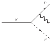
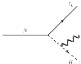
Figure 1: Feynman diagrams relevant for GW production from lepton and higgs leg.

Before we proceed for the evaluation of the spectrum of such GWs emitted during leptogenesis, it is pertinent to discuss the standard thermal leptogenesis scenario in the context of type-I seesaw Lagrangian presented in Eq. (1) so that its correlation with the emitted graviton energy density would become explicit. This Lagrangian naturally leads to the CP violating two body decay of heavy RHNs to the SM (anti-)lepton and (anti-)Higgs doublets. In the early Universe, these RHNs attain thermal equilibrium after being produced from the thermal bath via inverse decay (as long as $T\gg M_{i}$) as well as different scattering processes involving the gauge bosons and quarks. Subsequently, when the temperature drops down to $T\lesssim M_{i}$, the out-of-equilibrium decay of the $N_{i}$ generates a finite amount of CP asymmetry, parameterized by

$$\varepsilon_{\ell}^{i}=\frac{\Gamma(N_{i}\to\ell_{L}+H)-\Gamma(N_{i}\to\bar{\ell}_{L}+H^{\dagger})}{\Gamma(N_{i}\to\ell_{L}+H)+\Gamma(N_{i}\to\bar{\ell}_{L}+H^{\dagger})},$$ (5)

where the denominator denotes the total decay width of the RHN $N_{i}$ and is given by (at tree level):

$$\Gamma_{N_{i}}=M_{i}\frac{(Y_{\nu}^{\dagger}Y_{\nu})_{ii}}{8\pi}.$$ (6)

Note that the $1\rightarrow 3$ decay of RHN (via Eq. (3)) being suppressed by the Planck scale does not effectively contribute to this decay width (and $\varepsilon_{\ell}^{i}$) and hence excluded in evaluating the total decay width.

Assuming the minimal scenario with two hierarchical RHNs (say, $M_{1}\ll M_{2}$), the lepton asymmetry produced earlier from the decays of heavier $N_{2}$ gets diluted due to the prevailing production of the lightest RHN $N_{1}$ around $M_{2}>T>M_{1}$. As a consequence, only the lightest RHN $N_{1}$ decay (around $T\lesssim M_{1}$) effectively contributes to the generation of a non-vanishing CP asymmetry and can be expressed as

$$\varepsilon_{\ell}\equiv\varepsilon_{\ell}^{1}=\frac{1}{8\pi(Y_{\nu}^{\dagger}Y_{\nu})_{11}}\text{Im}\left[(Y_{\nu}^{\dagger}Y_{\nu})_{12}^{2}\right]\mathcal{F}\left(\frac{M_{2}^{2}}{M_{1}^{2}}\right),$$ (7)

where $\mathcal{F}(x)=\sqrt{x}\left[1+\frac{1}{1-x}+(1+x)\ln\left(\frac{x}{1+x}\right)\right]$ is the relevant loop function, generated as a result of the interference between one-loop diagram(s) and tree level decay, $N_{1}\to\ell_{L}+H$. Here the structure of CP-violating neutrino Yukawa coupling matrix $Y_{\nu}$ can be extracted using Casas-Ibarra (CI) parametrization [34] via:

$$Y_{\nu}=-i\frac{\sqrt{2}}{v}UD_{\sqrt{m}}{R}^{T}D_{\sqrt{M}}\,,$$ (8)

where $U$ is the Pontecorvo-Maki-Nakagawa-Sakata (PMNS) matrix which connects the flavor basis with mass basis for light neutrinos. $D_{\sqrt{m}}=\rm{diag}(\sqrt{m_{1}},\sqrt{m_{2}},\sqrt{m_{3}})$ is the diagonal matrix containing the square root of light neutrino mass and similarly $D_{\sqrt{M}}=\rm{diag}(\sqrt{M_{1}},\sqrt{M_{2}})$ represents the diagonal matrix for RHN masses. ${R}={R}(\theta)$ is an orthogonal matrix satisfying ${R}^{\rm{T}}{R}=1$ with $\theta$ being a complex angle.

To evaluate the exact amount of $B-L$ asymmetry generated from the CP violating out-of-equilibrium decay of the lightest RHN and its subsequent evolution $w.r.t$ time, one needs to solve the coupled Boltzmann Equations (BE) of the number density of the $N_{1}$ and $B-L$ asymmetry by incorporating the decay (and inverse decay) of $N_{1}$, as given by

$$\frac{dn_{N_{1}}}{dt}+3\mathcal{H}n_{N_{1}}=-(n_{N_{1}}-n_{N_{1}}^{\rm eq})\langle\Gamma_{N_{1}}\rangle-n_{N_{1}}\Gamma^{1\to 3}$$ (9)

$$\frac{dn_{B-L}}{dt}+3\mathcal{H}n_{B-L}=-\left[(n_{N_{1}}-n_{N_{1}}^{\rm eq})\varepsilon_{\ell}+n_{B-L}\frac{n_{N_{1}}^{\rm eq}}{n_{l}^{\rm eq}}\right]\langle\Gamma_{N_{1}}\rangle,$$ (10)

where $\langle\Gamma_{N_{1}}\rangle=\frac{K_{1}(z)}{K_{2}(z)}\Gamma_{N_{1}}$ is the thermal average of the decay rate of $N_{1}$ (via neutrino-Yukawa interaction only) with $K_{1},~{}K_{2}$ representing the Modified Bessel Functions of the 1st and 2nd kinds respectively while $z=M_{1}/T$ and $\mathcal{H}$ corresponds to the Hubble expansion parameter. Here $n_{N_{1}}^{(\rm eq)}=\frac{gT^{3}}{2\pi^{2}}\left(\frac{M_{1}}{T}\right)^{2}K_{2}(M_{1}/T)$ is the (equilibrium) number density of $N_{1}$ with $g$ being the number of degrees of freedom. The second term in the $r.h.s$ of Eq. (9) involving $1\rightarrow 3$ decay width of $N_{1}$ is kept, though insignificant for $N_{1}$ evolution, to indicate the production of gravitons from $N_{1}$ decay. Note that the corresponding inverse process is absent from the consideration that the gravitons have vanishing abundance compared to that of the elements of thermal bath initially.

For demonstration purpose, Fig. 2 shows the variation of $N_{1}$ and $B-L$ abundances as $Y_{N_{1}}=n_{N_{1}}/s,$ and $Y_{B-L}=n_{B-L}/s$ respectively, against the scale factor $A$ (normalized with respect to $a_{\rm RH}$ defined at reheating temperature, assuming an instantaneous reheating after the end of inflation, as part of initial conditions) of the Universe for a specific choice of $M_{1}=10^{10}$ GeV with $\rm Re[\theta]=0.9\pi$ and $\rm Im[\theta]=0.24$ while maintaining a hierarchy with other RHN, $M_{2}=10^{5}M_{1}$ (denoted as BP1). Note that the hierarchy among RHNs are chosen in such a way that they satisfy $M_{2}>T_{\rm RH}(\simeq 10^{14}~{}{\rm GeV})>M_{1}$, as a consequence of which the heavier RHNs $N_{2}$ are not expected to be present or produced during the entire evolution. The $Y_{\nu}$ is then obtained via Eq. (8) with $m_{1}=0$ and using the best fit values of neutrino oscillation parameters [38].

As can be seen from the nature of the blue curve, $N_{1}$ remains in thermal equilibrium in the early Universe and it starts to decay ($1\rightarrow 2$) thereafter. As a result of such decay of $N_{1}$, $Y_{B-L}$ (orange curve) starts to rise (neglecting the $\Gamma^{1\to 3}$ contribution) and finally saturates to a value around $A_{*}\sim 5\times 10^{5}$ (indicated by _∗, and a vertical dashed line in Fig. 2), representative of the correct baryon asymmetry of the Universe $Y_{B}^{\rm exp}=8.73\times 10^{-11}$ [39] via the relation, $Y_{B}=\frac{28}{79}Y_{B-L}$ [40]. The values of the specific $M_{1}$ and $\theta$ are so chosen to reproduce the correct baryon asymmetry. According to Davidson-Ibarra bound, such an evolution is expected for the $B-L$ asymmetry, provided $M_{1}\gtrsim 10^{9}$ GeV.

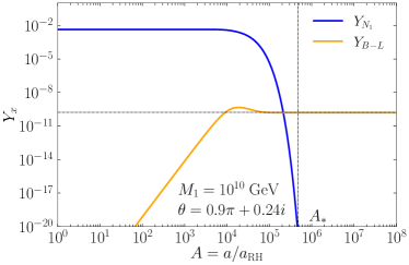
Figure 2: Evolution of $Y_{N_{1}}=n_{N_{1}}/s,$ and $Y_{B-L}=n_{B-L}/s$ $w.r.t$ rescaled scale factor $A=a/a_{\rm RH}$ where $a_{\rm RH}$ denotes the scale factor of the Universe when radiation energy density starts to dominate. Here $s$ denotes the entropy density of the Universe.

Note that while the three body decay of $N_{1}$ does not carry any direct impact on the generation and evolution of the $B-L$ asymmetry due to its origin being associated to a Planck scale suppressed interaction (via Eq. (3)) compared to the sizable neutrino-Yukawa coupling (responsible for two body decay of $N_{1}$ producing the $B-L$ asymmetry), this $1\rightarrow 3$ decay remains significant in contributing to the gravitational wave energy density produced during the $Y_{B-L}$ evolution, as we proceed to discuss below.

With the above understanding of the thermal leptogenesis scenario, we now turn our attention in obtaining the gravitational wave spectrum resulting during this leptogenesis era. To begin, we observe that the decay width of the lightest RHN toward three body final states involving a graviton, can conveniently be decomposed [41, 42] as:

$$\Gamma^{1\to 3} =\int\frac{d\Gamma^{1\to 3}}{dE_{k}}dE_{k},$$

$$= \int\frac{d\Gamma^{1\to 3}}{dE_{k}}\left[\frac{M_{1}-E_{k}}{M_{1}}\right]dE_{k}+\int\frac{d\Gamma^{1\to 3}}{dE_{k}}\left[\frac{E_{k}}{M_{1}}\right]dE_{k},$$ (11)

where $E_{k}(=2\pi f)$ is the energy (frequency) of the graviton spanning over the range $0<E_{k}\leq M_{1}/2$. The second term in $r.h.s$ isolates the decay contribution imparted to graviton alone, which would be helpful in determining the energy density of the GW, $\rho_{GW}$. After summing over the spins and polarizations, the differential decay width for $1\rightarrow 3$ process is found to be

$$\frac{d\Gamma^{1\to 3}_{grv}}{dE_{k}} =\frac{(Y_{\nu}^{\dagger}Y_{\nu})_{11}}{768\pi^{3}}\frac{M_{1}^{2}}{M_{p}^{2}}\mathcal{G}(x),$$ (12)

with $\mathcal{G}(x)=(2-x)(1-2x)^{2}/x$ and $x=M_{1}/T$. This result is obtained in the limit of unbroken electroweak symmetry at an early Universe for which all the SM fields were massless. In that case, it turns out that the sole contribution follows from the right Feynman diagram of Fig. 1 only, followed from the typical Lorentz structure of the SM interaction involving $SU(2)_{L}$ lepton doublet leading to the respective amplitude that is proportional to the mass of the lepton, as explained in the Supplemental Material.

Even though the lepton asymmetry calculation remains almost unaffected by the $1\rightarrow 3$ decay of $N_{1}$, the spectrum of gravitational wave is expected to be intricately related to $M_{1}$, or in other words, affected by the scale of leptogenesis due to its sole production (single graviton emission via bremsstrahlung) from $N_{1}$. This will be evident as we proceed further for calculation of the energy density of GW in the form of graviton radiation which satisfies the Boltzmann equation,

$$\frac{d\rho_{\rm GW}}{dt}+4\mathcal{H}\rho_{\rm GW}=\left[\int\frac{d\Gamma^{1\to 3}}{dE_{k}}\left(\frac{E_{k}}{M_{N}}\right)dE_{k}\right]n_{N_{1}}E_{N_{1}},$$ (13)

with $E_{N_{1}}=\sqrt{M_{1}^{2}+9T^{2}}$ representing the energy of the RHN in the thermal bath. With the understanding that the GW detectors are sensitive to different frequency domains, the above equation can conveniently be expressed in terms of differential energy density distribution $w.r.t$ the GW energy, defined by ${d\rho_{\rm GW}}/{dE_{k}}$, as

$$\frac{d}{dt}\left(\frac{d\rho_{\rm GW}}{dE_{k}}\right)+4\mathcal{H}\frac{d\rho_{\rm GW}}{dE_{k}}=\frac{E_{k}}{M_{N}}\frac{d\Gamma^{1\rightarrow 3}}{dE_{k}}n_{N_{1}}E_{N_{1}}.$$ (14)

The above equation can be solved for $[{d\rho_{\rm GW}}/{dE_{k}}]$ till a point where no further GW would be generated. In the present scenario, this point coincides to a stage where the Universe attained the normalized scale factor $A_{*}$ (at and beyond which $B-L$ asymmetry gets frozen, as stated earlier) indicative of the fact that $N_{1}$ decayed away completely. Taking into account the redshifts of the energy density as well as the energy of the graviton, the present day gravitational energy density $\Omega_{\rm GW}^{0}h^{2}$ can be inferred from the solution of Eq. (14) at $A_{*}$, described by $[{d\rho_{\rm GW}}/{dE_{k}}]_{*}$, as

$$\Omega_{\rm GW}^{0}h^{2} =\left[\frac{h^{2}}{\rho_{c}^{0}}E_{k}\frac{d\rho_{GW}}{dE_{k}}\right]_{\rm 0}=h^{2}\left(\frac{\Omega_{\gamma}^{0}}{\rho_{R}^{*}}\right)E_{k_{*}}\left[\frac{d\rho_{GW}}{dE_{k}}\right]_{*},$$ (15)

where $\Omega_{\gamma}^{0}=\rho_{R}^{0}/\rho_{c}^{0}=5.4\times 10^{-5}$ is the current relic density of photons and $E_{k_{*}}=E_{k}^{0}(A_{0}/A_{*})=E_{k}^{0}(\rho_{R}^{*}/\rho_{R}^{0})^{1/4}$ represents the energy of a single graviton at $A_{*}$ connected with the current energy of the same by $E_{k}^{0}=2\pi f^{0}$.

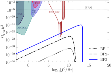
Figure 3: GW spectrum from RHN decaying to lepton doublet and Higgs when all the final state particle masses are taken to be zero. Here, BP-2(3): $[M_{1}=10^{13}~{}(10^{15})~{}\text{GeV},~{}M_{2}=10^{2}M_{1}~{}(5M_{1}),~{}\theta=0.51\pi+i0.05~{}(0.9\pi+i3.8\times 10^{-6})]$.

We include our findings for the GW in Fig. 3 for BP1 (BP2) where the dotted (dash-dotted) black line corresponds to the GW spectrum for $M_{1}=10^{10}(10^{13})$ GeV and $A_{*}=5\times 10^{5}~{}(480)$. In the same figure, we also embed future sensitivity ranges of space-based Laser interferometer experiments such as LISA [43], DECCIGO [44], CE [45] and LIGO [46] working in the intermediate frequency range, spanning over $10^{-6}-10^{4}$ Hz, as well as proposed resonant cavity techniques [47, 48] possibly probing higher frequency, ranging from $10^{4}$ to $10^{9}$ Hz. We find while the GW energy density $\Omega_{GW}h^{2}$ for $M_{1}=10^{10}$ GeV ($M_{2}$ and other parameters remain identical as in Fig. 2) falls way below the sensitivity regions of ongoing and future experiments, the one for $M_{1}=10^{13}$ GeV ($i.e.$, for BP2) enters marginally into the future sensitivity region of planned resonance cavity experiment. The corresponding peak frequency is found to be $6.1(6.7)\times 10^{10}$ Hz. Such a mild shift in peak frequency (while changing the mass of $M_{1}$ from $10^{10}$ GeV to $10^{13}$ GeV) is an artifact of the in-built changes in the neutrino Yukawa coupling $Y_{\nu}$ in order to realize correct amount of baryon asymmetry via leptogenesis, a characteristic of GW production during leptogenesis. A further increase in the GW energy density with $T>10^{13}$ GeV, though seems plausible by looking at the trend while moving from BP1 to BP2, is restricted in thermal leptogenesis at such high temperature, as stated earlier.

Based on the finding above, we notice that other leptogenesis scenarios which work with lighter RHNs such as resonant leptogenesis [3, 49], would only produce less GW energy density and hence the GW spectrum should fall below the sensitivity region of the planned and ongoing experiments in this case. On the other hand, for a non-thermal leptogenesis, the GWs produced via bremsstrahlung [50, 51, 41, 52, 53, 54] during the decay of the heavy particle ($e.g.$ inflaton) to RHNs [51] would be stronger, though do not carry the characteristic signature of leptogenesis, than those generated during the subsequent decay of the RHNs during non-thermal leptogenesis. Similarly, some alternate leptogenesis scenarios where GWs are generated due to the formation of domain walls [55], cosmic strings [56], bear the features of these exotic happenings rather than carrying signatures specific to the process of leptogenesis from RHN decay.

However a situation may prevail, where the (large) masses of the RHNs find their origin associated to a phase trasition (PT) in the early Universe at a temperature $T_{*}$. For example, there could be a bubble collision in case the PT being of first order that produces suddenly heavy RHNs (as they enter inside the bubble of true vacuum) [57, 58, 59, 60, 61] or there might be an interaction involving RHNs and a SM singlet scalar field $\phi$ of the form $\lambda_{i}\phi N_{i}N_{i}$, respecting a global $U(1)$ symmetry, for which RHNs become massive during a second order PT at $T_{*}$ with non-zero vacuum expectation value of $\phi$. In either case, provided masses of the RHNs turn out to be larger compared to $T_{*}$, they decay immediately. Such an instantaneous decay contributes not only to the production of lepton asymmetry but also to the production of GW via bremsstrahlung, similar to the preceding discussion.

To proceed with such sudden gain of mass for the RHNs due to PT, we first note that the RHNs (two here) were massless and part of the thermal bath prior to the PT, and suddenly both become massive at $T_{*}$. To be specific, if we consider the latter scenario describe above, we can employ the same Eq. (14) for finding out $\Omega_{GW}h^{2}$ contributed by both $N_{1,2}$ while replacing the initial (at the onset of PT) number density of the RHNs by their relativistic equilibrium number density, $n_{N_{i}}^{eq}$. We keep masses of $N_{1,2}$ close enough in this case so that there should not be much dilution due to the entropy production by the heavier component. We observe that $N_{1}$ of mass $10^{15}$ GeV, $M_{2}=5M_{1}$ with $T_{*}=10^{12}$ GeV can bring the GW spectrum well within the sensitivity range of proposed resonance cavity experiment (as shown in Fig. 3 by blue solid line) while generating the observed baryon asymmetry simultaneously. Note that as $T_{*}$ remains below $10^{13}$ GeV, the $\Delta L=2$ process $\ell_{L}+H\rightarrow\bar{\ell}_{L}+H^{\dagger}$ is not in equilibrium (which prevented us to go beyond $M_{1}>10^{13}$ GeV in case of thermal leptogenesis) and hence, a complete erasure of asymmetry by such process is no longer applicable. On the other hand, it is also observed that a significant increase of $M_{1,2}$ beyond $10^{16}$ GeV would introduce sizable elements, beyond the limit of perturbativity, of the neutrino Yukawa coupling.

Finally, to conclude, our study indicates that it is indeed possible to probe leptogenesis through GWs which were emitted in the form of graviton radiation during the out of equilibrium decay of heavy right handed neutrinos. In fact, the mechanism is not limited to the decay of RHNs only, rather the same can be extended to other leptogenesis scenarios [4, 5, 62, 63, 64, 65, 66, 67, 68, 69] involving heavy seesaw states like triplet scalars or fermions in the context of type-II [12, 70, 71, 72] or III [73] seesaw scenarios. At present, based on the proposed sensitivity range, it turns out that the resonant cavity experiment is capable of detecting such gravitational waves in case the seesaw state(s) be very heavy. However, with enhanced sensitivity range and planning of GW detectors at higher frequency range [47, 48], such probes of leptogenesis (and seesaw mechanism) can be extended for lighter seesaw states as well. Furthermore, as shown in a recent work of us [74], leptogenesis with RHNs having mass below the electroweak scale is also a possibility with temperature dependent heavy mass of RHNs at early Universe. Our present proposal is equally applicable to such scenarios also. Overall, the study of such GW spectrum associated to leptogenesis will open up several unexplored avenues for research in the field of leptogenesis which remains difficult to study at collider experiments because of the involvement of heavy seesaw states.

In this Supplemental Material, we plan to evaluate the differential decay rate (${d\Gamma}/{dE_{k}}$) of the three body decay process of the right handed neutrino (RHN) to the lepton and Higgs doublet with the possible emission of single graviton (double curly lines) as shown in Fig. 4.

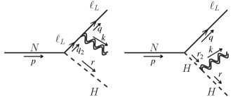
Figure 4: Feynman diagrams relevant for GW production from lepton and higgs leg.

The graviton being a massless spin-2 particle, the associated polarization tensors $\epsilon^{\mu\nu}_{i=1,2}$ satisfy the symmetric and transverse relations:

$$\epsilon_{i}^{\mu\nu} =\epsilon_{i}^{\nu\mu},~{}~{}k_{\mu}\epsilon_{i}^{\mu\nu}=0,$$ (16)

where $k=(E_{k},\bf{k})$ represents the graviton four momentum with $k^{2}=0$. Furthermore, they are traceless and orthonormal as specified by,

$$\eta_{\mu\nu}\epsilon_{i}^{\mu\nu} =0,\epsilon_{i}^{\mu\nu}\epsilon_{j_{\mu\nu}}=\delta_{ij},$$ (17)

where $\eta_{\mu\nu}$ is the flat metric. Additionally, summing over polarization indices provides

$$\sum_{pol.}\epsilon^{*\mu\nu}\epsilon^{\alpha\beta}=\frac{1}{2}\left[\hat{\eta}^{\mu\alpha}\hat{\eta}^{\nu\beta}+\hat{\eta}^{\mu\beta}\hat{\eta}^{\nu\alpha}-\hat{\eta}^{\mu\nu}\hat{\eta}^{\alpha\beta}\right],~{}\text{with}\hskip 10.00002pt\hat{\eta}^{\mu\nu}=\eta^{\mu\nu}-\frac{k_{\mu}\bar{k}_{\nu}+k_{\nu}\bar{k}_{\mu}}{k.\bar{k}}.$$ (18)

The massless nature of the graviton implies $k.\bar{k}=2E_{k}^{2}$ and $\bar{k}=(E_{k},-\bf{k})$.

To proceed for the evaluation of the differential decay rate, for simplification, a coordinate system is chosen in which the produced gravitons have momentum along $x$ direction, leading to $k=(E_{k},k_{x},0,0)$. Then, the four momentum of the decaying RHNs can be expressed as $p=(M_{i},0,0,0)$, while the four momentum associated to $\ell_{L}$ and $H$ take the form $q=(E_{q},q_{x},q_{y},q_{z}),~{}r=(M_{i}-E_{q}-E_{k},-q_{x}-k_{x},-q_{y},-q_{z})$ respectively. With these four vectors, the following relations are obtained:

$$p.p=M_{i}^{2},~{}~{}q.q=m_{l}^{2},~{}~{}r.r=m_{H}^{2},$$ (19)

$$p.q=M_{i}E_{q},~{}~{}p.r=M_{i}(M_{i}-E_{k}-E_{q}),~{}~{}p.k=p.\bar{k}=M_{i}E_{k},$$ (20)

$$q.r=\frac{1}{2}(M_{i}^{2}-2M_{i}E_{k}-(m_{l}^{2}+m_{H}^{2})),~{}~{}q.k=M_{i}(E_{k}+E_{q}-\frac{M_{i}}{2})+\frac{1}{2}(m_{H}^{2}-m_{l}^{2}),~{}~{}q.\bar{k}=2E_{q}E_{k}-q.k,$$ (21)

$$r.k=M_{i}E_{k}-q.k,~{}~{}q.\bar{k}=M_{i}E_{k}-2E_{q}E_{k}-2E_{k}^{2}+q.k\,,$$ (22)

which will be useful in calculating the differential decay width.

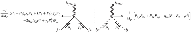
Figure 5: Feynman rules relevant for GW production from lepton and higgs leg.

We now move on to evaluate the Feynman amplitudes for both the diagrams of Fig. 4.

Since the RHNs interact only with the left handed lepton doublets $\ell_{L}$ and the SM Higgs $H$ via neutrino Yukawa interaction, gravitons can only emit (in the lowest order in $\kappa=2/M_{P}$) from either the left handed lepton side or the Higgs side as shown in left and right panels of Fig. 4 respectively. The relevant vertex factors can be derived from Eq. (3)-(4) of the main text and are presented in Fig. 5. Using the vertex factor involving $\ell_{L}\ell_{L}$-graviton presented in the left panel of Fig. 5 and the properties of the polarization tensor from Eq. (16) and (17), the Feynman amplitude for the $1\rightarrow 3$ decay of RHN (graviton being emitted from the lepton side) can be estimated as

$$\mathcal{M}_{1}=-\frac{Y_{\nu}q_{\mu}}{2M_{p}(q.k)}\left[\bar{u}_{\ell}(q)\gamma_{\nu}\mathbb{P}_{L}(\not{q_{2}}+m_{\ell})\mathbb{P}_{L}u_{N}^{c}(p)\right]\epsilon^{*\mu\nu},$$ (23)

while the one (with identical three body final states) for which graviton emission occurs from Higgs side is given by,

$$\mathcal{M}_{2}=-\frac{Y_{\nu}r_{\mu}r_{\nu}}{M_{p}(r.k)}\left[\bar{u}_{\ell}(q)\mathbb{P}_{L}u_{N}^{c}(p)\right]\epsilon^{*\mu\nu}.$$ (24)

Subsequently, using $q_{2}=k+q$, $(u_{N}^{c})^{\dagger}=-u_{N}^{T}\mathcal{C}^{\dagger}\gamma_{0}$ and $\sum_{s}\mathcal{C}\left[u_{N}(p)\bar{u}_{N}(p)\right]^{T}\mathcal{C}^{\dagger}=(-\not{p}+M_{i})$, the $\sum_{pol.}|\mathcal{M}_{1}|^{2}$ takes the form

$$\sum_{pol.}|\mathcal{M}_{1}|^{2} =-\frac{(Y_{\nu}^{\dagger}Y_{\nu})_{ii}}{4M_{p}^{2}(q.k)^{2}}\sum_{pol.}\epsilon^{\alpha\beta}\epsilon^{*\mu\nu}q_{\mu}q_{\beta}\text{Tr}\left[(\not{q}+m_{\ell})\gamma_{\nu}\mathbb{P}_{L}(\not{q_{2}}+m_{\ell})\mathbb{P}_{L}(-\not{p}+M_{i})\mathbb{P}_{R}(\not{q_{2}}+m_{\ell})\mathbb{P}_{R}\gamma_{\alpha}\right],$$ (25)

$$=\frac{m_{\ell}^{2}(Y_{\nu}^{\dagger}Y_{\nu})_{ii}}{4M_{p}^{2}E_{k}^{4}(q.k)^{2}}\left[E_{k}^{2}q^{2}-(q.k)(q.\bar{k})\right]\left[(p.q)(k.\bar{k}-2E_{k}^{2})-\{(q.k)(p.\bar{k})+(q.\bar{k})(p.k)\}\right].$$ (26)

Similarly, for the $1\rightarrow 3$ decay process of the RHN where graviton emission takes place from the Higgs side (right diagram of Fig. 4), the squared Feynman amplitude is given by

$$\sum_{pol.}|\mathcal{M}_{2}|^{2} =\frac{(Y_{\nu}^{\dagger}Y_{\nu})_{ii}2(p.q)}{(r.k)^{2}M_{p}^{2}}\sum_{pol.}\epsilon^{\alpha\beta}\epsilon^{*\mu\nu}r_{\alpha}r_{\beta}r_{\mu}r_{\nu}=\frac{(Y_{\nu}^{\dagger}Y_{\nu})_{ii}(p.q)}{(r.k)^{2}M_{p}^{2}}\left[r^{2}-\frac{(r.k)(r.\bar{k})}{E_{k}^{2}}\right]^{2}.$$ (27)

There should also exist interference term $\mathcal{M}_{1}\mathcal{M}_{2}^{*}$, which is estimated as

$$\sum_{pol.}\mathcal{M}_{1}\mathcal{M}_{2}^{*}=\frac{m_{l}^{2}(Y_{\nu}^{\dagger}Y_{\nu})_{ii}}{M_{p}^{2}(q.k)(r.k)}\Bigg{[}2\Bigg{\{}p.r-\frac{(p.\bar{k})(r.k)+(p.k)(r.\bar{k})}{2E_{k}^{2}}\Bigg{\}}\Bigg{\{}q.r-\frac{(q.k)(r.\bar{k})+(r.k)(q.\bar{k})}{2E_{k}^{2}}\Bigg{\}}$$

$$-\Bigg{\{}r^{2}-\frac{(r.k)(r.\bar{k})}{E_{k}^{2}}\Bigg{\}}\Bigg{\{}p.q-\frac{(p.\bar{k})(q.k)+(q.\bar{k})(p.k)}{2E_{k}^{2}}\Bigg{\}}\Bigg{]}.$$ (28)

Note that both $|\mathcal{M}_{1}|^{2}$ and $M_{1}M_{2}^{*}$ depend on the final state lepton mass $m_{\ell}$. However, for the scenario we pursue in this work, the RHNs are required to decay (due to their heavy mass) far above the electroweak phase transition where the electroweak symmetry was unbroken. Hence, contribution of $|\mathcal{M}_{1}|^{2}$ and $M_{1}M_{2}^{*}$ vanish in the zero mass of the leptons. As a result, the $1\rightarrow 3$ decay of the RHNs essentially depend on the $|\mathcal{M}_{2}|^{2}$.

The differential decay rate then can be evaluated as

$$\frac{d\Gamma}{dE_{k}} =\frac{1}{8M_{i}}\frac{1}{(2\pi)^{3}}\int_{E_{q,min}}^{E_{q,max}}\sum_{pol.}\left(|\mathcal{M}_{1}|^{2}+|\mathcal{M}_{2}|^{2}+2|\mathcal{M}_{1}\mathcal{M}_{2}^{*}|\right)dE_{q},$$ (29)

where the limits of the integration is given by

$$E_{q,max/q,min}=\frac{M_{i}}{2(1-2x)}\left[(1-3x+2x^{2}-y_{1}^{2}+xy_{1}^{2}+y_{2}^{2}-xy_{2}^{2})\pm x\alpha\right],$$

$$\alpha=\left(1-4x+4x^{2}-2y_{1}^{2}+4xy_{1}^{2}+y_{1}^{4}-2y_{2}^{2}+4xy_{2}^{2}-2y_{1}^{2}y_{2}^{2}+y_{2}^{4}\right)^{1/2},$$ (30)

with $x=E_{k}/M_{i}$, $y_{1}=m_{H}/M_{i}$ and $y_{2}=m_{l}/M_{i}$. Finally, in zero mass limit of Higgs and leptons i.e., $y_{1}=y_{2}\rightarrow 0$, the differential decay rate of the three body decay process of RHNs takes the form

$$\frac{d\Gamma}{dE_{k}} =\frac{M_{i}^{2}(Y_{\nu}^{\dagger}Y_{\nu})_{ii}(2-x)(1-2x)^{2}}{768M_{p}^{2}\pi^{3}x},$$ (31)

as presented in Eq. (12).