Universal bounds in quantum metrology in presence of correlated noise

Abstract

We derive fundamental bounds for general quantum metrological models involving both temporal or spatial correlations (mathematically described by quantum combs), which may be effectively computed in the limit of a large number of probes or sensing channels involved. Although the bounds are not guaranteed to be tight in general, their tightness may be systematically increased by increasing numerical complexity of the procedure. Interestingly, this approach yields bounds tighter than the state of the art also for uncorrelated channels. We apply the bound to study the limits for the most general adaptive phase estimation models in the presence of temporally correlated dephasing. We consider dephasing both parallel (no Heisenberg scaling) and perpendicular (Heisenberg scaling possible) to the signal. In the former case our new bounds show that negative correlations are beneficial, for the latter we show evidence that the bounds are tight.

Introduction.

Contrasting the effects of noise is the foremost challenge in advancing quantum technologies [1]. All real-world quantum systems are influenced by environmental interactions that lead to decoherence, particle losses, etc. In principle, even under these conditions, quantum advantage can often be achieved with the help of quantum error correction (QEC) codes [2].

In quantum metrology [3, 4, 5, 6, 7, 8, 9, 10, 11, 12, 13], the most spectacular type of quantum advantage is the Heisenberg scaling (HS), for which the precision scales as $1/N$, where $N$ is the number of quantum resources (such as particles or channel uses), whereas for standard scaling (SS) the precision is proportional to $1/\sqrt{N}$. Strategies to attain the HS are known for noiseless [14, 3] and noisy [15, 16, 17] phase estimation—in the latter case, proper QEC is indispensable. For the majority of noise types the HS is unattainable—nevertheless, entanglement or QEC assisted protocols often allow to significantly improve the constant in SS.

The recent developments in quantum channel estimation theory allow to fully characterize the ultimate precision limits in the presence of all types of uncorrelated noise—it is possible to determine whether a given model exhibits HS or SS, and calculate an asymptotically tight formula for precision via a simple semidefinite program (SDP) [18, 19, 20, 21, 22, 23, 17, 24, 25, 26, 27].

Nevertheless, noise and signal correlations play important role in many physical systems [28, 29, 30, 31, 32, 33, 34, 35, 36, 37]. In numerous works, case studies of the performance of specific estimation strategies in the presence of various types of correlated noise were carried out, for temporal [38, 39, 40, 41, 42, 43, 44, 45, 46] and spatial [47, 48, 49, 50, 51, 52] correlations, or both [53, 54]. However, universal methods that provide fundamental bounds (also in the asymptotic regime of large resources) for quantum metrological models in presence of correlated noise are missing. As such, one cannot judge whether the precision given by the protocols studied is close to optimal or not. In this work, we fill this gap and show universal methods to derive fundamental bounds for correlated noise models.

State-of-the-art bounds

Numerous metrological tasks, e.g. phase estimation or super-resolution imaging [55], boil down to the estimation of a single, real parameter $\theta$—the goal is to find its (locally) unbiased estimator $\tilde{\theta}$ with minimal variance $\Delta^{2}\tilde{\theta}$. When the parameter is encoded in $\theta$-dependent quantum mixed state $\rho_{\theta}$, then a quantum Cramér-Rao Bound (QCRB) says that $\Delta^{2}\tilde{\theta}\geq\frac{1}{F(\rho_{\theta})}$, where $F(\rho_{\theta})$ is the quantum Fisher information (QFI) [56, 57] (we recall the definition of the QFI in Appendix A ). The QFI is a local quantity that depends only on the state $\rho_{\theta}$ and its derivative $\dot{\rho}_{\theta}=\partial_{\theta}\rho_{\theta}$ evaluated at some specific value of $\theta$ around which the estimation is performed.

Let $\ket{\Psi_{\theta}}$ be a purification of $\rho_{\theta}$: $\rho_{\theta}=\text{Tr}_{\mathcal{E}}(\ket{\Psi_{\theta}}\bra{\Psi_{\theta}})$, $\mathcal{E}$ is a space added for purification purposes. Obviously, $F(\ket{\Psi_{\theta}})\geq F(\rho_{\theta})$ because any generalized measurement feasible with $\rho_{\theta}$ can be done on extended state $\ket{\Psi_{\theta}}$. Interestingly, for any $\rho_{\theta}$ one can find a QFI non-increasing purification (QFI NIP) satisfying [18, 58]

$$F(\ket{\Psi_{\theta}})=F(\rho_{\theta}),\quad\braket{\Psi_{\theta}}{\dot{\Psi}_{\theta}}=0.$$ (1)

The existence of QFI NIP together with a simple formula for pure state QFI, $F(\ket{\Psi_{\theta}})=4(\braket{\dot{\Psi}_{\theta}}{\dot{\Psi}_{\theta}}-|\braket{\Psi_{\theta}}{\dot{\Psi}_{\theta}}|^{2})$, leads to a very useful general formula,

$$F(\rho_{\theta})=4\min_{\ket{\Psi_{\theta}}}\braket{\dot{\Psi}_{\theta}}{\dot{\Psi}_{\theta}},$$ (2)

where minimization is taken over all purifications of $\rho_{\theta}$.

In quantum channel estimation theory, a parameter $\theta$ is encoded in a quantum channel (CPTP map) $\Lambda_{\theta}(\bullet)=\sum_{k}K_{k,\theta}\bullet K_{k,\theta}^{\dagger}$, where $K_{k,\theta}$ are Kraus operators [20]. We can probe the channel using a system living in a Hilbert space $\mathcal{H}$, possibly entangled with an ancillary system ($\mathcal{A}$), then the output state of probe and ancilla is given by $\rho_{\theta}=(\Lambda_{\theta}\otimes\mathcal{I}_{\mathcal{A}})(\rho)$, where $\rho\in\mathcal{L}(\mathcal{H}\otimes\mathcal{A})$ is a joint input state of probe and ancillary systems, $\mathcal{L}(\bullet)$ is the set of linear operators acting on $\bullet$. The ultimate precision of $\theta$ estimation is then quantified by the channel QFI

$$\mathcal{F}(\Lambda_{\theta})=\max_{\rho}F(\rho_{\theta}).$$ (3)

This maximization is arduous using brute-force techniques, but can be efficiently done with the help of (2) because minimization over output state purifications boils down to minimization over Kraus representations of $\Lambda_{\theta}$ [18]:

$$\mathcal{F}(\Lambda_{\theta})=4\min_{h}\|\alpha\|,\quad\alpha=\sum_{k}\dot{\tilde{K}}^{\dagger}_{k,\theta}\dot{\tilde{K}}_{k,\theta},$$ (4)

where $\|\bullet\|$ is an operator norm, $h$ is a hermitian matrix generating different Kraus representations according to a rule $\dot{\tilde{K}}_{k,\theta}=\dot{K}_{k,\theta}-ih_{kk^{\prime}}K_{k^{\prime},\theta}$, the summation is performed over repeated index. It can be shown, that minimization over $h$ is equivalent to minimization over all Kraus representations, and that (4) can be translated to a simple SDP [20].

The real potential of quantum metrology can be exploited when $N>1$ channel copies are probed collectively using adaptive or active quantum feedback (AD) strategies, where channels $\Lambda_{\theta}:\mathcal{L}(\mathcal{H}_{2i-1})\rightarrow\mathcal{L}(\mathcal{H}_{2i})$ for $i\in\{1,2,...,N\}$ are probed sequentially, and arbitrary quantum control channels $\textrm{C}_{i}:\mathcal{L}(\mathcal{H}_{2i}\otimes\mathcal{A}_{i})\rightarrow\mathcal{L}(\mathcal{H}_{2i+1}\otimes\mathcal{A}_{i+1})$ can act on a probe and arbitrarily large ancilla $\mathcal{A}_{i}$ after each $\Lambda_{\theta}$, see Fig. 1. The AD class covers all estimation strategies apart from those involving indefinite causal order [60]—in particular, parallel strategies, when a large entangled state probes all $N$ channels simultaneously, form a subset of AD [22].

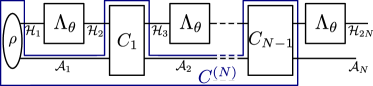
Figure 1: General adaptive (AD) scheme probing $N$ independent copies of a channel $\Lambda_{\theta}$. The input state $\rho$ and intermediate control channels $C_{i}$ can be represented as a quantum comb $C$.

General quantum AD strategy can be represented by a single Choi-Jamiołkowski (CJ) operator called a quantum comb [61]. The set of quantum combs $\textrm{Comb}[(\mathcal{K}_{1},\mathcal{K}_{2}),...,(\mathcal{K}_{2N-1},\mathcal{K}_{2N})]$ consists of positive semidefinite operators $E$ for which there exists a sequence of operators $E^{(k)}$ for $k=1,...,N$ such that $E=E^{(N)}$,

$$\textrm{Tr}_{2k}E^{(k)}=E^{(k-1)}\otimes\mathbb{1}_{2k-1}\quad\textrm{for}\quad k=2,...,N,$$ (5)

$\textrm{Tr}_{2}(E^{(1)})=\mathbb{1}_{1}$, Hilbert spaces $\mathcal{K}_{2k-1},\mathcal{K}_{2k}$ can be interpreted as input/output of $k$th comb tooth respectively.

Controls $\textrm{C}_{i}$ together with an input state $\rho$ form a comb $C^{(N)}\in\text{Comb}[(\emptyset,\mathcal{H}_{1}),(\mathcal{H}_{2},\mathcal{H}_{3}),...,(\mathcal{H}_{2N-2},\mathcal{H}_{2N-1}\otimes\mathcal{A}_{N})]$, where $\emptyset$ represents a trivial space (the first tooth has no input), we use roman font for channels, and italics for corresponding CJ operators. The probed channels can be represented as a comb as well, $\varLambda_{\theta}^{(N)}\in\text{Comb}[(\mathcal{H}_{1},\mathcal{H}_{2}),...,(\mathcal{H}_{2N-1},\mathcal{H}_{2N})]$. A general comb $\varLambda_{\theta}^{(N)}$ can model any type of noise and signal correlations, whereas for uncorrelated models it reduces to $\varLambda_{\theta}^{(N)}=\varLambda_{\theta}^{\otimes N}$.

To calculate the output state $\rho_{\theta}\in\mathcal{L}(\mathcal{H}_{2N}\otimes\mathcal{A}_{N})$, we should concatenate the corresponding inputs and outputs of $C^{(N)}$ and $\varLambda_{\theta}^{(N)}$, which can be done using a link product operation, $\rho_{\theta}=C^{(N)}\star\varLambda_{\theta}^{(N)}$, see Refs. [61, 62] for more details. The adaptive channel QFI or comb QFI, defined as [45]

$$\mathcal{F}_{\text{AD}}^{(N)}=\max_{C^{(N)}}F(C^{(N)}\star\varLambda_{\theta}^{(N)}),$$ (6)

quantifies the ultimate precision when arbitrary AD strategy can be used to sense a parameter encoded in a comb $\varLambda_{\theta}^{(N)}$.

To calculate $\mathcal{F}_{\text{AD}}^{(N)}$ for small $N$, one should first decompose $\varLambda_{\theta}^{(N)}=\sum_{k}\ket{K_{k,\theta}^{(N)}}\bra{K_{k,\theta}^{(N)}}$, where $\ket{K_{k,\theta}^{(N)}}$ are vectorized Kraus operators—this decomposition is not unique. Then, analogously to $\alpha$, defined in (4), a performance operator can be defined as $\tilde{\Omega}_{\Lambda}^{(N)}=\text{Tr}_{\text{out}}\left(\sum_{k}\ket{\dot{\tilde{K}}_{k,\theta}^{(N)}}\bra{\dot{\tilde{K}}_{k,\theta}^{(N)}}\right)$ , where $\text{Tr}_{\text{out}}$ is the partial trace over the last output space of $\varLambda_{\theta}^{(N)}$ ($\mathcal{H}_{2N}$), $\ket{\dot{\tilde{K}}_{k,\theta}^{(N)}}=\ket{\dot{K}_{k,\theta}^{(N)}}-ih_{kk^{\prime}}\ket{{K}_{k^{\prime},\theta}^{(N)}}$, $h$ is a hermitian matrix. Then the maximization in (6) can be written as [45, 60]

$$\max_{C^{(N)}}F(C^{(N)}\star\varLambda_{\theta}^{(N)})=4\min_{h}\max_{\tilde{C}^{(N)}}\text{Tr}\left(\tilde{\Omega}_{\Lambda}^{(N)}\tilde{C}^{(N)}\right),$$ (7)

where $\tilde{C}^{(N)}=\text{Tr}_{\mathcal{A}_{N}}C^{(N)}$.

The RHS of this equation can be formulated as a single SDP after translating maximization over $\tilde{C}^{(N)}$ to minimization using strong duality [45, 60]. Unfortunately, the complexity of the resulting problem grows exponentially with $N$, which makes it intractable for $N\gtrsim 5$.

In the case of uncorrelated noise models, one can go around this problem, and for large $N$ instead of calculating the exact value of $\mathcal{F}_{\text{AD}}$ compute the bounds, using the following iteration [27]

$$\mathcal{F}_{\text{AD}}^{(i+1)}\leq\mathcal{F}_{\text{AD}}^{(i)}+4\min_{h}\left[\|\alpha\|+\sqrt{\mathcal{F}_{\text{AD}}^{(i)}}\|\beta\|\right],$$ (8)

where $\beta=\sum_{k}\dot{\tilde{K}}_{k}^{\dagger}K_{k}$, (see Ref. [27] for initial and Appendix B.1 for a simplified derivation). Note that if there exists $h$ for which $\beta=0$, $\mathcal{F}_{\text{AD}}^{(N)}$ will scales at most linearly with $N$. Hence we can write:

$$\lim_{N\rightarrow\infty}\mathcal{F}_{\text{AD}}^{(N)}/N\leq 4\min_{h}\|\alpha\|\leavevmode\nobreak\ \leavevmode\nobreak\ \text{s.t.}\leavevmode\nobreak\ \leavevmode\nobreak\ \beta=0$$ (9)

On the other hand, when $\beta\neq 0$ for all $h$, then the HS is in principle allowed, and the asymptotic form of (8) reads

$$\lim_{N\rightarrow\infty}\mathcal{F}_{\text{AD}}^{(N)}/N^{2}\leq 4\min_{h}\|\beta\|^{2}.$$ (10)

The iterative bound (8) and asymptotic bounds (9), (10) can be formulated as SDPs [21, 27]. Interestingly, even though the bound (8) is not tight in general, its asymptotic forms (9) and (10) are always saturable, even using narrower class of parallel strategies instead of general AD strategies [26].

Bound for correlated noise

In what follows we derive bounds analogous to (8), (9), (10) valid for all correlated noise models, and efficiently calculable for arbitrarily large $N$.

Our results are complementary to Refs. [64, 65], where tensor network comb representation was used to find optimal AD estimation strategies in the presence of correlated noise for big ($N\approx 50$) number of channels. The introduced procedure searches through a subclass of adaptive strategies (involving limited ancilla size), and consequently returns a lower bound of $\mathcal{F}_{\text{AD}}$. Our novel upper bound allows in particular to benchmark the optimality of strategies found using this approach.

The comb $\varLambda_{\theta}^{(N)}$ representing a correlated noise metrological model can be viewed as a link product of CJ operators of its teeth $\overset{\leftrightarrow}{\Lambda}_{\theta}:\mathcal{L}(\mathcal{H}_{2i-1}\otimes\mathcal{R}_{i-1})\rightarrow\mathcal{L}(\mathcal{H}_{2i}\otimes\mathcal{R}_{i})$ for $i\in\{1,2,...,N\}$, where $\mathcal{R}_{i}$ are inaccessible environmental spaces carrying information needed to model correlations, the fixed state $\sigma_{\text{in}}$ is an input of the first register $\mathcal{R}_{0}$, the last register $\mathcal{R}_{N}$ is traced out—see Fig. 2(a). The $\leftrightarrow$ symbol in $\overset{\leftrightarrow}{\Lambda}_{\theta}$ indicates the presence of unconcatenated environmental spaces. As in the uncorrelated case, we assume subsequent teeth are identical, but the reasoning may be extended beyond this assumption. Let $\rho_{\theta}^{(l)}\in\mathcal{L}(\mathcal{H}_{2l}\otimes\mathcal{R}_{l}\otimes\mathcal{A}_{l})$ describe joint probe, ancilla and environment state after the action of $l$ teeth of $\varLambda_{\theta}^{(N)}$ and let $F^{(i)}:=F(\rho_{\theta}^{(i)})$.

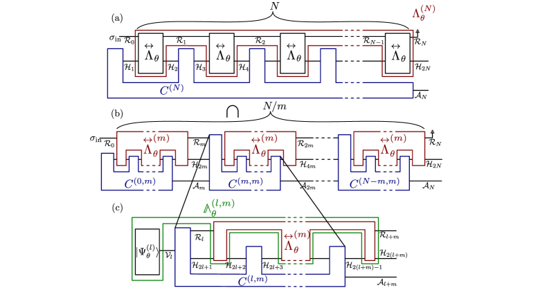
Figure 2: Any comb $\varLambda_{\theta}^{(N)}$ can be represented as a link product of its teeth $\overset{\leftrightarrow}{\varLambda}_{\theta}$, physically implementable estimation strategies $C^{(N)}$ control probe subspaces $\mathcal{H}$ only (a). To derive an iterative upper bound, we divide $\varLambda_{\theta}^{(N)}$ into blocks of $m$ teeth $\overset{\leftrightarrow}{\varLambda}_{\theta}^{(m)}$, and allow to additionally control register $\mathcal{R}$ after each block (b). In each iteration step (12), we concatenate the purified state of probe, register and ancilla ($\mathcal{A}$) after $l$ channel uses $\ket{\Psi_{\theta}^{(l)}}$ with next $m$ channels $\overset{\leftrightarrow}{\varLambda}_{\theta}^{(m)}$and compute the maximal QFI of a resulting comb $\mathbb{\Lambda}_{\theta}^{(l,m)}$ (c).

Our goal is to upper bound $F^{(l+m)}$ given $F^{(l)}$, where $\rho_{\theta}^{(l+m)}$ is created by evolving $\rho_{\theta}^{(l)}$ through subsequent $m$ teeth of $\varLambda_{\theta}^{(N)}$ represented by $\overset{\leftrightarrow}{\varLambda}_{\theta}^{(m)}$, see Fig. 1(b,c), where again the symbol $\leftrightarrow$ indicates that the first input and last output of this comb contain environmental spaces. The evolution can be accompanied by a general adaptive quantum control.

To simplify the bound derivation, let us assume that we have access to $\ket{\Psi_{\theta}^{(l)}}$, which is a QFI NIP of $\rho_{\theta}^{(l)}$ satisfying (1) ($\mathcal{E}_{l}$ is an additional space added for purification). This assumption can only increase $F^{(l+m)}$, since all tasks doable with a state can be also done with its purification. Let us combine $\ket{\Psi_{\theta}^{(l)}}$ and $\overset{\leftrightarrow}{\varLambda}_{\theta}^{(m)}$ into a single $\theta$-dependent comb $\mathbb{\Lambda}_{\theta}^{(l,m)}=\ket{\Psi_{\theta}^{(l)}}\bra{\Psi_{\theta}^{(l)}}\otimes\overset{\leftrightarrow}{\varLambda}_{\theta}^{(m)}$.

The comb QFI of $\mathbb{\Lambda}_{\theta}^{(l,m)}$ is an upper bound for $F^{(l+m)}$ since $\rho_{\theta}^{(l+m)}=\mathbb{\Lambda}_{\theta}^{(l,m)}\star C^{(l,m)}$, where $C^{(l,m)}$ is a control comb with labeled inputs and outputs of subsequent teeth as shown in Fig. 1(c).

To calculate the comb QFI, one needs to know the comb and its derivative—therefore, apart from $\overset{\leftrightarrow}{\varLambda}_{\theta}^{(m)}$ and $\dot{\overset{\leftrightarrow}{\varLambda}}_{\theta}^{(m)}$, which can be directly computed for a given noise model, we need to specify $\ket{\Psi_{\theta}^{(l)}}$ and $\ket{\dot{\Psi}_{\theta}^{(l)}}$ . Fortunately, $F^{(l)}$ defines $\ket{\Psi_{\theta}^{(l)}}$ and $\ket{\dot{\Psi}_{\theta}^{(l)}}$ up to a unitary rotation—those two vectors span a two dimensional subspace (sometimes called a virtual qubit [66]) $\mathcal{V}_{l}\subset\mathcal{H}_{2l}\otimes\mathcal{A}_{l}\otimes\mathcal{R}_{l}\otimes\mathcal{E}_{l}$, and vectors $\ket{0}=\ket{\Psi_{\theta}^{(l)}}$, $\ket{1}=2\ket{\dot{\Psi}_{\theta}^{(l)}}/\sqrt{F^{(l)}}$ form an o.-n. basis of $\mathcal{V}_{l}$—the orthonormality can be proven using (1) and pure state QFI formula. Using $\{\ket{0},\ket{1}\}$ basis we can write:

$$\ket{\Psi_{\theta}^{(l)}}=\begin{bmatrix}1\\ 0\\ \end{bmatrix},\quad\ket{\dot{\Psi}_{\theta}^{(l)}}=\begin{bmatrix}0\\ \sqrt{F^{(l)}}/2\\ \end{bmatrix}.$$ (11)

There is no need to specify $\ket{0}$ and $\ket{1}$—it is enough to know, that for some $\ket{0}$, $\ket{1}$ relations (11) hold. We can then set the first input space of $C^{(l,m)}$ to be $\mathcal{V}_{l}$ since only this subspace is relevant.

The maximal value of $F^{(l+m)}$ is an upper bound for $\mathcal{F}_{\text{AD}}^{(l+m)}$, and consequently

$$\mathcal{F}_{\text{AD}}^{(l+m)}\leq\max_{C^{(l,m)}}F(C^{(l,m)}\star\mathbb{\Lambda}_{\theta}^{(l,m)}),\leavevmode\nobreak\ \leavevmode\nobreak\ \mathbb{\Lambda}_{\theta}^{(l,m)}=\begin{bmatrix}1&0\\ 0&0\\ \end{bmatrix}\otimes\overset{\leftrightarrow}{\varLambda}_{\theta}^{(m)},\\ \dot{\mathbb{\Lambda}}^{(l,m)}_{\theta}=\begin{bmatrix}1&0\\ 0&0\\ \end{bmatrix}\otimes\dot{\overset{\leftrightarrow}{\varLambda}}_{\theta}^{(m)}+\frac{\sqrt{\mathcal{F}_{\text{AD}}^{(l)}}}{2}\begin{bmatrix}0&1\\ 1&0\\ \end{bmatrix}\otimes\overset{\leftrightarrow}{\varLambda}_{\theta}^{(m)}.$$ (12)

The registers $\mathcal{R}_{0}$ and $\mathcal{R}_{N}$ are closed, so the first and last iteration steps must be modified accordingly. The bound might not be tight for several reasons: (i) the state $\rho_{\theta}^{(l+m)}$ contains environment $\mathcal{R}_{l+m}$ apart from accessible probe and ancilla subsystems; (ii) $C^{(l,m)}$ acts on inaccessible environmental space $\mathcal{R}_{l}$; (iii) $\rho_{\theta}^{(i)}$ is replaced with its purification every $m$ steps. In a physical AD scheme, the environment is always directly sent to a next tooth of $\varLambda_{\theta}^{(N)}$, but (i) and (ii) mean that we allow for arbitrary operation acting on environment every $m$ teeth. This is the price to pay for dividing $N$ correlated channels into smaller blocks of $m$, while keeping the universal validity of the bound at the same time—neglecting the information contained in environment may lead to incorrect, underestimated bound.

The procedure (12) may be also applied to uncorrelated noise models—then, (iii) is the only reason for the bound untightness, which makes it at least as tight as the old one given by (8) . The new bound can be strictly tighter (for finite $N$) than the old one even for $m=1$, increasing $m$ tightens the bound (12) even more—see Appendix B.2. However, for $N\rightarrow\infty$, the bounds are asymptotically equivalent (and saturable) irrespectively of $m$ chosen.

For correlated noise, the role of $m$ is more significant, since information leaks from environment every $m$ steps, and increasing $m$ tightens the bound also asymptotically.

To get an asymptotic form of the correlated noise bound, we rephrase the maximization problem from (12) using (7), and then expand a performance operator of $\mathbb{\Lambda}_{\theta}^{(l,m)}$ ($\tilde{\Omega}_{\mathbb{\Lambda}}^{(l,m)}$) using (11) (see Appendix C.1) to get

$$\text{Tr}(\tilde{\Omega}_{\mathbb{\Lambda}}^{(l,m)}\tilde{C}^{(l,m)})=\frac{F^{(l)}}{4}+\text{Tr}\left(\tilde{\Omega}^{(m)}_{\Lambda}\tilde{C}_{00}\right)+\\ +\sqrt{F^{(l)}}\text{Re}\left(\text{Tr}\left(\boldsymbol{\beta}^{(m)}\tilde{C}_{10}\right)\right),$$ (13)

where $\tilde{\Omega}_{\Lambda}^{(m)}$ is a performance operator of $\overset{\leftrightarrow}{\varLambda}_{\theta}^{(m)}$, $\ket{K_{k,\theta}^{(m)}}$ are its vectorized Kraus operators (we dropped symbol $\leftrightarrow$), $\boldsymbol{\beta}^{(m)}=\text{Tr}_{\text{out}}\left(\sum_{k}\ket{\dot{\tilde{K}}_{k,\theta}^{(m)}}\bra{{K}_{k,\theta}^{(m)}}\right)$, $\tilde{C}^{(l,m)}=\text{Tr}_{\mathcal{A}_{l+m}}C^{(l,m)}$ and $\tilde{C}_{ij}=\prescript{}{\mathcal{V}_{l}}{\braket{i}{\tilde{C}^{(m+l)}}{j}}_{\mathcal{V}_{l}}$. The maximization of the LHS of (13) over $\tilde{C}^{(l,m)}$ can be upper-bounded my maximizing each term of the RHS independently, which leads to

$$\mathcal{F}_{\text{AD}}^{(l+m)}\leq\mathcal{F}_{\text{AD}}^{(l)}+4\min_{h}\left[\max_{\tilde{C}^{\text{A}}}\text{Tr}\left(\tilde{\Omega}^{(m)}_{\Lambda}\tilde{C}^{\text{A}}_{00}\right)+\right.\\ \left.+\sqrt{\mathcal{F}_{\text{AD}}^{(l)}}\max_{\tilde{C}^{\text{B}}}\text{Re}\left(\text{Tr}\left(\boldsymbol{\beta}^{(m)}\tilde{C}_{10}^{\text{B}}\right)\right)\right],$$ (14)

$\tilde{C}^{\text{A}}$, $\tilde{C}^{\text{B}}$ are independent combs of the same type as $\tilde{C}^{(m+l)}$, superscript ^(m+l) was dropped for conciseness.

The two maximization problems in the RHS of (14) do not depend on $l$, so we can adopt convention $l=0$ for naming the subspaces on which operators $\tilde{C}_{ij}$, $\boldsymbol{\beta}^{(m)}$ and $\tilde{\Omega}_{\Lambda}^{(m)}$ act. Let $\mathcal{X}_{m}$ be a linear space of traceless operators satisfying the linear conditions (5), where $\mathcal{K}_{1},...,\mathcal{K}_{2m}$ are subsequent input and output spaces of combs $\tilde{C}_{ij}$, so $\mathcal{K}_{1}=\emptyset$, $\mathcal{K}_{2}=\mathcal{H}_{1}\otimes\mathcal{R}_{0}$, $\mathcal{K}_{3}=\mathcal{H}_{2}$, … ,$\mathcal{K}_{2m}=\mathcal{H}_{2m-1}$, and let $\mathcal{X}_{m}^{\perp}$ be the orthogonal complement of $\mathcal{X}_{m}$ in the space of all operators with respect to Hilbert-Schmidt scalar product. Then, we can uniquely decompose $\boldsymbol{\beta}^{(m)}=\boldsymbol{\beta}^{(m)}_{1}+\boldsymbol{\beta}^{(m)}_{2}$, where $\boldsymbol{\beta}^{(m)}_{1}\in\mathcal{X}_{m}$, $\boldsymbol{\beta}_{2}^{(m)}\in\mathcal{X}_{m}^{\perp}$. Since $\tilde{C}_{10}^{\dagger}\in\mathcal{X}_{m}$ , we have $\textrm{Tr}(\boldsymbol{\beta}_{2}^{(m)}\tilde{C}_{10}^{\text{B}})=0$, and consequently $\boldsymbol{\beta}^{(m)}$ can be replaced with $\boldsymbol{\beta}_{1}^{(m)}$ in (14). Moreover, as we prove in Appendix C.1, the maximization over $\tilde{C}^{\textrm{B}}$ in (14) always returns non-negative number, which is equal to $0$ iff $\boldsymbol{\beta}^{(m)}_{1}=0$ for a given $h$. If such $h$ exists, then the QFI scales at most linearly:

$$\lim_{N\rightarrow\infty}\mathcal{F}_{\text{AD}}^{(N)}/N\leq 4\min_{h}\max_{\tilde{C}}\text{Tr}\left(\tilde{\Omega}^{(m)}_{\Lambda}\tilde{C}_{00}\right)/m\leavevmode\nobreak\ \leavevmode\nobreak\ \text{s.t.}\leavevmode\nobreak\ \leavevmode\nobreak\ \boldsymbol{\beta}^{(m)}_{1}=0.$$ (15)

If such $h$ does not exists, then the HS is allowed by the bound:

$$\lim_{N\rightarrow\infty}\mathcal{F}_{\text{AD}}^{(N)}/N^{2}\leq 4\min_{h}\left[\max_{\tilde{C}}\text{Re}\left(\text{Tr}\left(\boldsymbol{\beta}_{1}^{(m)}\tilde{C}_{10}\right)/m\right)\right]^{2}.$$ (16)

In Appendix C.2 we show how to translate bounds (12), (15) and (16) into single SDPs using the technique from Refs. [45, 60]. The bound became less tight after replacing a common maximization from (12) with two maximizations in (14)—however, as we show in Appendix C.1, this has no impact asymptotically, and the bounds (15), (16) are asymptotically equivalent to (12) iterated many times. These asymptotic bounds are not guaranteed to be tight, though they can be made tighter by increasing $m$.

Example: correlated dephasing

To illustrate the practical relevance of this new family of bounds, we consider the example of phase estimation in the presence of correlated dephasing noise. Single-qubit dephasing is manifested as a shrinkage of the Bloch vector by a factor $\eta=\cos(\epsilon)$ towards axis parallel to unit vector $\vec{n}$. It can be interpreted as a rotation of a qubit by a random angle $+\epsilon$ or $-\epsilon$ around axis $\vec{n}$, each angle is picked with equal probability $1/2$, $\epsilon\in[0,\pi/2]$. The corresponding noise Kraus operators are $K_{+}=R_{\vec{n}}({+\epsilon})/\sqrt{2},\quad K_{-}=R_{\vec{n}}({-\epsilon})/\sqrt{2}$, where $R_{\vec{n}}(\varphi)=e^{-\frac{i}{2}\varphi\vec{n}\cdot\vec{\sigma}}$, $\vec{\sigma}=[\sigma_{x},\sigma_{y},\sigma_{z}]$, the Kraus operators including the unitary signal are $K_{\pm,\theta}=R_{\hat{z}}(\theta)K_{\pm}$ (we assume that noise acts before signal).

To investigate a basic form of correlations, we assume that the rotational directions for consecutive dephasing channels are elements of a binary Markov chain, where the conditional probability of rotational direction $s_{i}\in\{+,-\}$ in channel $i$ assuming direction $s_{i-1}$ in channel $i-1$ is given by

$$T_{i|i-1}(s_{i}|s_{i-1})=(1+s_{i}s_{i-1}C)/2,$$ (17)

where $i\in\{2,3,...,N\}$ , $C\in[-1,1]$ is a correlation parameter: $C=0$ corresponds to no correlations, $C=1$ means maximal positive correlations, and $C=-1$—maximal negative correlations. In the first channel both directions are equally probable, $p_{1}(+)=p_{1}(-)=1/2$.

We can model the correlations by interwinding unitaries $V_{\theta}$ acting on probe ($\mathcal{H}$) and register ($\mathcal{R}$) qubits with mixing operations $T$ acting on $\mathcal{R}$ only [64], see Fig. 3(a).

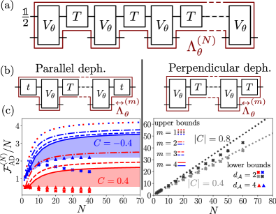
Figure 3: Binary correlations between dephasing channels can be modeled using scheme (a). To get the tightest possible bound, the chain of correlated channels should be cut into pieces differently for parallel and perpendicular dephasing (b). The precision limits for both cases are shown in (c). For the case of parallel dephasing, we shaded the regions between the lower and upper bounds of the QFI per channel achievable with up to $N$ coherent channel uses. The resulting areas for negative ($C=-0.4$, blue) and positive ($C=0.4$, red) correlations are disjoint, which proves that negative correlations offer fundamental metrological advantage over positive correlations. For perpendicular dephasing, the QFI depends on $|C|$, but not on its sign. For two studied cases ($|C|=0.4,|C|=0.8$) we observe that the upper bounds are equally tight for all $N$ for $m\in\{1,2,3\}$, which suggest that the bounds are tight for $m=1$. Moreover, for $|C|=0.4$ it is possible to almost saturate the bound already with one-qubit ancilla.

The register contains the information about the next direction of rotation—if found in a state $\ket{\pm}$, rotation $R_{\vec{n}}({\pm\epsilon})$ is performed; $\ket{+}$, $\ket{-}$ are an o.-n. basis of $\mathcal{R}$. The unitary operation acting on $\mathcal{H}\otimes\mathcal{R}$ is $V_{\theta}=\sqrt{2}K_{+,\theta}\otimes\ket{+}_{\mathcal{R}}\bra{+}+\sqrt{2}K_{-,\theta}\otimes\ket{-}_{\mathcal{R}}\bra{-}.$ The Kraus operators of channel $T$ are $T_{sr}=\sqrt{\frac{1+srC}{2}}\ket{s}\bra{r}$ for $s,r\in\{+,-\}$, so it applies the classical map (17) on the basis $\ket{\pm}$ of $\mathcal{R}$.

To calculate the bound, we need to cut the whole chain $\Lambda_{\theta}^{(N)}$ into pieces $\overset{\leftrightarrow}{\Lambda}_{\theta}^{(m)}$. This can be done in many different ways, the choice affects the tightness of the bound.

Let us consider the parallel dephasing case $\vec{n}=\hat{z}$, when noise commutes with signal. If we cut a chain after $T$ and before $V_{\theta}$, we get a full control on the sign of $\epsilon$ for the first dephasing channel in each block—this results in apparent HS manifested by the bound. If we cut a chain after $U$ and before $T$, then we get information about the sign of the rotation of the last channel in each block, which also leads to apparent HS.

To resolve this issue, we cut the chain in the middle of the operation $T$—we write a classical map $T$ as a concatenation of two maps $t$ given by conditional probabilities

$$t_{i|i-1}(s_{i}|s_{i-1})=(1+s_{i}s_{i-1}\sqrt{|C|})/2,$$ (18)

when $C<0$, then a bit flip on basis $\ket{\pm}$ has to be additionally inserted between two operations $t$. The resulting comb $\overset{\leftrightarrow}{\Lambda}_{\theta}^{(m)}$ consists of $m$ unitaries $V_{\theta}$ intertwined with mixing channels $T$, with channels $t$ (performing the classical operation (18) on the basis $\ket{\pm}_{\mathcal{R}}$) at both ends, see Fig. 3(b). We insert $\overset{\leftrightarrow}{\Lambda}_{\theta}^{(m)}$ into the iterative procedure (12) to derive a bound, which is valid for a scenario when each two neighboring unitaries $V_{\theta}$ are connected by $T$. For the first iteration step we send the maximally mixed state as input for the register.

We numerically observe that the HS is not possible for correlated parallel dephasing for any $-1<C<1$ and $0\leq\eta<1$. In Fig. 3 we compare upper bounds, calculated for positive ($C=0.4$) and negative ($C=-0.4$) correlations, with lower bounds—QFIs achievable using protocols with small ancilla dimension $d_{\mathcal{A}}$, calculated using tensor networks based algorithm described in Ref. [64]. These bounds can be made arbitrarily tight by increasing $m$ and $d_{\mathcal{A}}$, respectively; however, this quickly becomes numerically costly. We managed to perform calculations up to $d_{\mathcal{A}}=4$ and $m=4$, for these values the lower and upper bounds still do not coincide. Nevertheless, for the first time we find precision limits of metrological protocols with arbitrarily large $d_{\mathcal{A}}$ applicable to correlated noise. This allows us to deduce that negative correlations offer metrological advantage over positive correlations.

Let us also study the perpendicular dephasing case ($\vec{n}=\hat{x}$), for which the HS is possible [27]. As we checked numerically, to get the tightest bound in this case, we should not split the noisy operations $T$ in the blocks’ boundaries equally—instead, we should make a cut after $V_{\theta}$ and before $T$, see Fig. 3(b). This is because non-commuting noise acts before the signal, and the information about dephasing direction is no longer useful after the signal. Interestingly, the resulting bounds are equally tight for $m\in\{1,2,3\}$, which suggests that the bound is already tight for $m=1$. We confirm this by observing that the QFI achievable by adaptive protocol with $d_{\mathcal{A}}=2$ is very close to the upper bound calculated for $m=1$, see Fig. 3(c). We checked, that for perpendicular dephasing the QFI does not depend on the sign of $C$, but on its absolute value—correlations may be used as an extra source of information, since the achievable precision increases with $|C|$.

Conclusions.

The examples presented above are just a small sample of the numerous possible applications of this new family of bounds. The introduced formalism allows for handling not only classical but also inherently quantum correlations between subsequent channels, which arise in the study of non-Markovian open quantum systems [29, 30, 32, 34]. Although the sequential scheme, where channels occur one after another, suggests a focus on temporal correlations, the bound is also valid for spatial correlations. In these cases, channels are usually sampled in parallel, but since parallel schemes are a subset of adaptive ones, the bound still holds.

The presented results are also important for uncorrelated quantum metrology, since the derived bound is stronger (or at least equally strong) then the state-of-the art bound [27] even in its simplest, single-channel version ($m=1$). The bound can be made arbitrarily tight by increasing the iteration step $m$.

This work, together with [64, 65], establishes a comprehensive framework to study metrological protocols in the presence of correlated noise for a large number of probed channels. In the near future, we plan to apply this framework to get new insights about real-life scenarios [68], and to explore the effects of inherently quantum environments, e.g. in collisional quantum thermometry [69, 70].

A challenging extension will be to explore the continuous time limit, where quantum combs (also known as process tensors [34]) are routinely used in numerical studies of the dynamics and control of non-Markovian open systems [32, 71, 72, 73, 74]. Finally, it will be interesting to see if similar ideas apply to the related problem of discriminating quantum combs [75, 76, 77, 78].

Acknowledgements.

We thank Wojciech Górecki and Andrea Smirne for helpful discussions. This work was supported by the National Science Center (Poland) grant No.2020/37/B/ST2/02134. FA acknowledges support from Marie Skłodowska-Curie Action EUHORIZON-MSCA-2021PF-01 (project QECANM, grant No. 101068347).

Appendix A Basics of Quantum Fisher Information

The QFI of an arbitrary mixed state $\rho_{\theta}$ can be calculated using the formula

$$F(\rho_{\theta})=\textrm{Tr}(\rho_{\theta}L_{\theta}^{2}),\quad\dot{\rho}_{\theta}=\frac{1}{2}\left(\rho_{\theta}L_{\theta}+L_{\theta}\rho_{\theta}\right),$$ (19)

where dot denotes the derivative over $\theta$, and the symmetric logarithmic derivative (SLD) matrix $L_{\theta}$ can be calculated by solving the rightmost equation from (19). For pure state models $\rho_{\theta}=\ket{\psi_{\theta}}\bra{\psi_{\theta}}$, the closed analytical formula for SLD and the QFI can be easily derived:

$$L_{\theta}=2\left(\ket{\dot{\psi}_{\theta}}\bra{\psi_{\theta}}+\ket{\psi_{\theta}}\bra{\dot{\psi}_{\theta}}\right),\quad F(\ket{\psi_{\theta}})=4(\braket{\dot{\psi}_{\theta}}{\dot{\psi}_{\theta}}-|\braket{\psi_{\theta}}{\dot{\psi}_{\theta}}|^{2}).$$ (20)

Appendix B Uncorrelated noise bound

The bound (8) has been derived in Ref. [27], and the asymptotic bounds (9) and (10) are its direct consequences, see (11), (12) from Ref. [27]. In what follows, we provide a simpler derivation of (8). From the new derivation it is clear, that the bound generated by (12) for uncorrelated noise is at least as tight as the one given by (8). The advantage of the old derivation is that it can be easily generalized to strategies involving causal superpositions.

B.1 Simplified derivation

We consider an AD scheme in which $N$ independent channels $\Lambda_{\theta}$ are probed—we keep the notation from the main text. Let $\rho_{\theta}^{(l)}\in\mathcal{L}(\mathcal{H}_{2l}\otimes\mathcal{A}_{l})$ be the probe and ancilla state after $l$th use of $\Lambda_{\theta}$, let $F(\rho_{\theta}^{(l)})=F^{(l)}$. The state after the next control is $\text{C}_{l}(\rho_{\theta}^{(l)})$, we construct its QFI NIP $\ket{\Psi_{\theta}^{(l)}}\in\mathcal{H}_{2l+1}\otimes\mathcal{A}_{l+1}\otimes\mathcal{E}_{l}$, where $\mathcal{E}_{l}$ is an artificial space added for purification purposes. Using (1) and (20) and the fact that $\theta$-independent channel cannot increase the QFI [58, p. 57], we obtain

$$4\braket{\dot{\Psi}_{\theta}^{(l)}}{\dot{\Psi}_{\theta}^{(l)}}=F(\text{C}_{l}(\rho_{\theta}^{(l)}))\leq F^{(l)}.$$ (21)

Let $\bar{K}_{k,\theta}=K_{k,\theta}\otimes\mathbb{1}_{\mathcal{A}_{l+1}\otimes\mathcal{E}_{l}}$, the state of probe and ancilla after the action of the $(l+1)$th channel can be written as

$$\rho_{\theta}^{(l+1)}=\textrm{Tr}_{\mathcal{E}_{l}}\left(\sum_{k}\bar{K}_{k,\theta}\ket{\Psi_{\theta}^{(l)}}\bra{\Psi_{\theta}^{(l)}}\bar{K}_{k,\theta}^{\dagger}\right).$$ (22)

Since the QFI of a subsystem is smaller or equal than the QFI of the whole system (i) and the QFI of a purification is larger or equal than the QFI of a purified state (ii), we obtain

$$F^{(l+1)}\overset{(\textrm{i})}{\leq}F\left(\sum_{k}\bar{K}_{k,\theta}\ket{\Psi_{\theta}^{(l)}}\bra{\Psi_{\theta}^{(l)}}\bar{K}_{k,\theta}^{\dagger}\right)\overset{(\textrm{ii})}{\leq}F\left(\sum_{k}\bar{K}_{k,\theta}\ket{\Psi_{\theta}^{(l)}}\otimes\ket{k}_{\mathcal{E^{\prime}}_{l}}\right),$$ (23)

where $\mathcal{E^{\prime}}_{l}$ is an additional space added for purification, vectors $\ket{k}_{\mathcal{E^{\prime}}_{l}}$ form its o.-n. basis. After expanding the rightmost part of (23) using (20), we obtain

$$F^{(l+1)}/4 \leq\bra{\dot{\Psi}_{\theta}^{(l)}}\sum_{k}\bar{K}^{\dagger}_{\theta,k}\bar{K}_{\theta,k}\ket{\dot{\Psi}_{\theta}^{(l)}}+\bra{\dot{\Psi}_{\theta}^{(l)}}\sum_{i}\bar{K}^{\dagger}_{\theta,k}\dot{\bar{K}}_{\theta,k}\ket{\Psi_{\theta}^{(l)}}+\bra{\Psi_{\theta}^{(l)}}\sum_{i}\dot{\bar{K}}^{\dagger}_{\theta,k}{\bar{K}}_{\theta,k}\ket{\dot{\Psi}_{\theta}^{(l)}}+$$ (24)

$$+\bra{\Psi_{\theta}^{(l)}}\sum_{i}\dot{\bar{K}}^{\dagger}_{\theta,k}\dot{\bar{K}}_{\theta,k}\ket{\Psi_{\theta}^{(l)}}$$ (25)

From (21) and identity $\sum_{k}\bar{K}^{\dagger}_{\theta,k}\bar{K}_{\theta,k}=\mathbb{1}$ we deduce that the first term is upper bounded by $F^{(l)}/4$; the last term is upper-bounded by $\|\alpha\|$ because $\braket{\Psi_{\theta}^{(l)}}{\Psi_{\theta}^{(l)}}=1$ and $\|A\otimes\mathbb{1}\|=\|A\|$. Both the 2nd and the 3rd term are upper-bounded by $\sqrt{F^{(l)}/4}\|\beta\|$, this follows from the inequality

$$\braket{x}{A}{y}\leq\sqrt{\braket{x}{x}}\|A\|\sqrt{\braket{y}{y}},$$ (26)

which is a weaker version of (7) from [27]. After taking this all together, we obtain (8).

To derive this bound, we assumed the access to QFI NIP of a probe and ancilla after each control. Moreover, we maximized each term of (24) independently—this is another factor making the bound not tight, since usually all the terms cannot be maximal at the same time. Interestingly, to derive (12), we only assumed the access the access to QFI NIP every $m$ steps, no additional assumptions were required. Therefore, the bound generated by (12) is guaranteed to be at least as tight as the one generated by (8) already for $m=1$. Increasing $m$ may tighten the bound even more.

B.2 Example

To illustrate the effectiveness of a bound, let us calculate it for $m\in\{1,2,3\}$ for phase estimation in the presence of amplitude damping noise, for which $K_{k,\theta}=K_{k}e^{-\frac{i\theta\sigma_{z}}{2}}$,

$$K_{1}=\ket{0}\bra{0}+\sqrt{p}\ket{1}\bra{1},\quad K_{2}=\sqrt{1-p}\ket{0}\bra{1}.$$ (27)

In Fig. 4, we demonstrate the results for $p=0.5$. The newly introduced bound is tighter than the old one already for $m=1$ . For larger $m$, the bound becomes even tighter, and very close to the optimal QFI calculated exactly for $m\leq 4$ using the algorithm from Ref. [45].

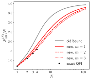
Figure 4: Precision bounds for phase estimation in the presence of amplitude damping noise.

Appendix C Correlated noise bound

C.1 Asymptotic bounds: the derivation details

To derive the asymptotic bounds (9), (10), (15), (16) using iteration relations (8) and (14), we will use the following lemma.

Lemma 1 Let $a^{(n)}$ be a sequence of real numbers satisfying $a^{(n+1)}=a^{(n)}+A+2B\sqrt{a^{(n)}}$ for any integer $n$, $a^{(0)}=0$, $A\geq B^{2}$. Then

$$\lim_{n\rightarrow\infty}a^{(n)}/n=A\leavevmode\nobreak\ \leavevmode\nobreak\ \textrm{for}\leavevmode\nobreak\ \leavevmode\nobreak\ B=0;\quad\lim_{n\rightarrow\infty}a^{(n)}/n^{2}=B^{2}\leavevmode\nobreak\ \leavevmode\nobreak\ \textrm{for}\leavevmode\nobreak\ \leavevmode\nobreak\ B\geq 0.$$ (28)

Proof When $B=0$, then $a^{(n)}=An$, so the first part of lemma is obvious. When $B>0$, then for any $n\geq 1$

$$a^{(n)}\leq f(n)=An+B^{2}n(n-1)+(A-B^{2})n\log n,$$ (29)

which is proven in the supplementary material of Ref. [27], Appendix E, in which $\|\alpha\|$ and $\|\beta\|$ play the role of $A$ and $B$. Let us now prove that for any $n\geq 1$

$$a^{(n)}\geq B^{2}n^{2}.$$ (30)

This can be shown by induction, we have $a^{(1)}=A\geq B^{2}1^{2}$, and when (30) holds for some $n$, then for $n+1$ we have

$$a^{(n+1)}\geq B^{2}n^{2}+2B^{2}n+A\geq B^{2}n^{2}+2B^{2}n+B^{2}=B^{2}(n+1)^{2}.$$ (31)

From (29) , (30), and the fact that $\lim_{n\rightarrow\infty}f(n)/n^{2}=B^{2}$ follows the 2nd part of the lemma. $\blacksquare$

The asymptotic bounds for uncorrelated noise (9) and (10) are direct consequences of the iterative bound (8) and Lemma 1—notice that asymptotically (for large $\mathcal{F}_{\text{AD}}^{(i)}$) the minimum over $h$ is always achieved when $\|\beta\|$ is minimal, since it is multiplied by $\sqrt{\mathcal{F}_{\text{AD}}^{(i)}}$ and consequently eventually dominates over the term with $\|\alpha\|$, unless $\|\beta\|=0$.

Let us proceed to the derivation of (13). Since $\overset{\leftrightarrow}{\varLambda}_{\theta}^{(m)}=\sum_{k}\ket{K_{k,\theta}^{(m)}}\bra{K_{k,\theta}^{(m)}}$ and $\mathbb{\Lambda}_{\theta}^{(l,m)}=\ket{\Psi_{\theta}^{(l)}}\bra{\Psi_{\theta}^{(l)}}\otimes\overset{\leftrightarrow}{\varLambda}_{\theta}^{(m)}$, we can decompose

$$\mathbb{\Lambda}_{\theta}^{(l,m)}=\sum_{k}\ket{L_{k,\theta}^{(l,m)}}\bra{L_{k,\theta}^{(l,m)}},$$ (32)

where $\ket{L_{k,\theta}^{(l,m)}}=\ket{\Psi_{\theta}^{(l)}}\otimes\ket{K_{k,\theta}^{(m)}}$. Using Leibniz rule and (11) we obtain

$$\ket{{L}_{k,\theta}^{(l,m)}}=\ket{0}\otimes\ket{{K}_{k,\theta}^{(m)}},\quad\ket{\dot{L}_{k,\theta}^{(l,m)}}=\ket{0}\otimes\ket{\dot{K}_{k,\theta}^{(m)}}+\sqrt{F^{(l)}}/2\ket{1}\otimes\ket{K_{k,\theta}^{(m)}},$$ (33)

and consequently $\ket{\dot{\tilde{L}}_{k,\theta}^{(l,m)}}=\ket{0}\otimes\ket{\dot{\tilde{K}}_{k,\theta}^{(m)}}+\sqrt{F^{(l)}}/2\ket{1}\otimes\ket{K_{k,\theta}^{(m)}}$, where $\ket{\dot{\tilde{L}}_{k,\theta}^{(l,m)}}=\ket{\dot{L}_{k,\theta}^{(l,m)}}-ih_{kk^{\prime}}\ket{{L}_{k^{\prime},\theta}^{(l,m)}}$ for some hermitian matrix $h$. After inserting this into the definition of the performance operator we get

$$\tilde{\Omega}^{(l,m)}_{\mathbb{\Lambda}}=\text{Tr}_{\text{out}}\left(\sum_{k}\ket{\dot{\tilde{L}}_{k,\theta}^{(l,m)}}\bra{\dot{\tilde{L}}_{k,\theta}^{(l,m)}}\right)=\ket{0}\bra{0}\otimes\tilde{\Omega}_{\Lambda}^{(m)}+\frac{1}{2}\sqrt{F^{(l)}}\ket{0}\bra{1}\otimes\boldsymbol{\beta}^{(m)}+\frac{1}{2}\sqrt{F^{(l)}}\ket{1}\bra{0}\otimes\boldsymbol{\beta}^{(m)\dagger}+\frac{1}{4}F^{(l)}\ket{1}\bra{1}\otimes\tilde{\varLambda}^{(m)},$$ (34)

where $\tilde{\varLambda}^{(m)}=\text{Tr}_{\text{out}}\overset{\leftrightarrow}{\varLambda}_{\theta}^{(m)}$, here $\text{Tr}_{\text{out}}$ is the partial trace over the subspace $\mathcal{H}_{2(l+m)}\otimes\mathcal{R}_{l+m}$, which is the last output of $\overset{\leftrightarrow}{\varLambda}_{\theta}^{(m)}$. After decomposing $\tilde{C}^{(m,l)}=\sum_{i,j=0}^{1}\ket{i}_{\mathcal{V}_{l}}\bra{j}\otimes\tilde{C}_{ij}$, using (34) and the normalization condition $\text{Tr}(\tilde{C}_{11}\tilde{\varLambda}^{(m)})=\tilde{C}_{11}\star\varLambda^{(m)}=1$, we obtain (13). The normalization condition was derived using the fact that $\tilde{C}_{11}\in\text{Comb}[(\emptyset,\mathcal{H}_{2l+1}\otimes\mathcal{R}_{l}),(\mathcal{H}_{2l+2},\mathcal{H}_{2l+3}),...,(\mathcal{H}_{2(l+m)-2},\mathcal{H}_{2(l+m)-1})]$ and $\tilde{\varLambda}^{(m)}\in\text{Comb}[(\mathcal{H}_{2l+1}\otimes\mathcal{R}_{l},\mathcal{H}_{2l+2}),(\mathcal{H}_{2l+3},\mathcal{H}_{2l+4}),...,(\mathcal{H}_{2(l+m)-1},\emptyset)]$, so all outputs of $\tilde{C}_{11}$ are inputs of $\tilde{\Lambda}^{(m)}$ and vice versa.

The upper bound for $\mathcal{F}_{\text{AD}}^{(l+m)}$ is obtained by maximizing the RHS of (13) over $\tilde{C}^{(l+m)}$ ($F^{(l)}$ should be replaced with the upper bound for $\mathcal{F}_{\text{AD}}^{(l)}$). To further simplify the bound, we maximize each term independently (we use the inequality between the maximum of sum and the sum of maxima), which leads to (14). This step may weaken the bound for finite $N$, but, interestingly, it does not affect its asymptotic behavior. To show this, let us consider two cases:

1. Heisenberg scaling is possible. Then, for $F^{(l)}\rightarrow\infty$ the last term of the RHS of (13) dominates over the middle one. When we pick $\tilde{C}^{(l+m)}$ such that $\tilde{C}_{10}$ maximizes the last term, then the result of a maximization over $\tilde{C}^{(l+m)}$ is arbitrarily close to the result of independent maximization over $\tilde{C}^{A}$, $\tilde{C}^{B}$ for $F^{(l)}\rightarrow\infty$ (the ratio between the two results $\rightarrow 1$).

2. Heisenberg scaling is not possible. Then, to minimize the figure of merit over $h$ for $F^{(l)}\rightarrow\infty$, we should choose $h$ for which the last term of (13) is $0$ for any $\tilde{C}_{10}$. Then, we can choose $\tilde{C}_{10}=0$ without affecting the result. This makes the condition $\tilde{C}^{(l+m)}\succeq 0$ equivalent to $\tilde{C}_{00},\tilde{C}_{11}\succeq 0$ , so the coupling between the two maximization problems is again irrelevant.

Let us introduce the following notation:

$$\lambda_{\text{A}}(h)=4\max_{\tilde{C}^{\text{A}}}\text{Tr}\left(\tilde{\Omega}^{(m)}_{\Lambda}\tilde{C}^{\text{A}}_{00}\right),\quad\lambda_{\text{B}}(h)=2\max_{\tilde{C}^{\text{B}}}\text{Re}\left(\text{Tr}\left(\boldsymbol{\beta}^{(m)}\tilde{C}_{10}^{\text{B}}\right)\right),$$ (35)

so we can write (14) as

$$\mathcal{F}_{\text{AD}}^{(l+m)}\leq\mathcal{F}_{\text{AD}}^{(l)}+\min_{h}\left[\lambda_{\text{A}}(h)+2\lambda_{\text{B}}(h)\sqrt{\mathcal{F}^{(l)}_{\text{AD}}}\right]$$ (36)

To derive corresponding asymptotic bounds, let us firstly derive a sufficient and necessary condition for vanishing of $\lambda_{\text{B}}(h)$. We use the decomposition $\bm{\beta}^{(m)}=\bm{\beta}_{1}^{(m)}+\bm{\beta}_{2}^{(m)}$, see the main text below (14), and prove the following lemma.

Lemma 2 $\lambda_{\text{B}}(h)\geq 0$, moreover $\lambda_{\text{B}}(h)=0$ if and only if $\bm{\beta}_{1}^{(m)}=0$.

Proof The comb conditions for $\tilde{C}^{\text{B}}$ are equivalent to the following set of conditions for its blocks $\tilde{C}^{\text{B}}_{ij}$ (from now on we will use subspaces naming convention $l=0$ as in the main text): (i) $\tilde{C}^{\text{B}}_{00},\tilde{C}^{\text{B}}_{11}\in\text{Comb}[(\emptyset,\mathcal{H}_{1}\otimes\mathcal{R}_{0}),(\mathcal{H}_{2},\mathcal{H}_{3}),...,(\mathcal{H}_{2m-2},\mathcal{H}_{2m-1})]$; (ii) $\tilde{C}^{\text{B}}_{01},\tilde{C}^{\text{B}}_{10}\in\mathcal{X}_{m}$; (iii) $\tilde{C}^{\text{B}}_{01}=\tilde{C}^{\text{B}\dagger}_{10}$ and $\tilde{C}^{\text{B}}_{00}\succeq\tilde{C}^{\text{B}\dagger}_{10}\left(\tilde{C}^{\text{B}}_{11}\right)^{-1}\tilde{C}^{\text{B}}_{10}$. When $\tilde{C}^{\text{B}}_{11}$ is singular, then its inverse should be replaced with pseudo inverse in the proofs of lemmas 2 and 3. The space $\mathcal{X}_{m}$ is defined below (14), conditions (i) and (ii) are a consequence of the linear constraints for the comb $\tilde{C}^{(l,m)}$, and condition (iii) is a consequence of the positivity constraint and Shur’s complement condition. If we choose any $\tilde{C}_{00}^{\text{B}}$, $\tilde{C}_{11}^{\text{B}}$ satisfying (i) and set $\tilde{C}^{\text{B}}_{01}=\tilde{C}^{\text{B}}_{10}=0$, then conditions (ii)-(iii) are also satisfied and $\text{Tr}\left(\boldsymbol{\beta}^{(m)}\tilde{C}_{10}^{\text{B}}\right)=0$ which proves that $\lambda_{\text{B}}(h)\geq 0$. Since for all cases $\tilde{C}^{\text{B}\dagger}_{10}\in\mathcal{X}_{m}$ and $\bm{\beta}_{2}^{(m)}\in\mathcal{X}_{m}^{\perp}$, we have $\text{Tr}\left(\tilde{C}^{\text{B}}_{10}\bm{\beta}_{2}^{(m)}\right)=0$, so $\lambda_{\text{B}}(h)=0$ when $\bm{\beta}_{1}^{(m)}=0$. Let us now assume that $\bm{\beta}_{1}^{(m)}\neq 0$, and fix strictly positive definite $\tilde{C}^{\text{B}}_{00}$ and $\tilde{C}^{\text{B}}_{11}$ satisfying condition (i), and $\tilde{C}_{01}^{\text{B}}=\epsilon\bm{\beta}_{1}^{(m)}$, $\tilde{C}_{10}^{\text{B}}=\epsilon\bm{\beta}_{1}^{(m)\dagger}$. Then, condition (ii) is satisfied since $\bm{\beta}_{1}^{(m)}\in\mathcal{X}_{m}$, and for small enough $\epsilon>0$ condition (iii) is also satisfied since $\tilde{C}_{00}^{\text{B}}$ is strictly positive. Therefore, there exists a comb $\tilde{C}^{\text{B}}$ for which $\text{Re}\left(\text{Tr}\left(\boldsymbol{\beta}^{(m)}\tilde{C}_{10}^{\text{B}}\right)\right)=\epsilon\text{Re}\left(\text{Tr}\left(\boldsymbol{\beta}_{1}^{(m)}\boldsymbol{\beta}_{1}^{(m)\dagger}\right)\right)>0$, which finishes the proof of the 2nd part of the lemma. $\blacksquare$

Furthermore, let us generalize the inequality $\|\alpha\|\geq\|\beta\|^{2}$ to the case of correlated noise.

Lemma 3 $\lambda_{\text{A}}(h)\geq\lambda_{\text{B}}(h)^{2}$

Proof Let us use the notation $\tilde{C}^{\text{A}}$, $\tilde{C}^{\text{B}}$ for matrices maximizing $\lambda_{\text{A}}(h)$ and $\lambda_{\text{B}}(h)$ respectively. Obviously, $\lambda_{\text{A}}(h)\geq 4\text{Tr}\left(\tilde{\Omega}^{(m)}_{\Lambda}\tilde{C}^{\text{B}}_{00}\right)$ and $\lambda_{\text{B}}(h)^{2}\leq 4\left|\text{Tr}\left(\boldsymbol{\beta}^{(m)}\tilde{C}_{10}^{\text{B}}\right)\right|^{2}$, so the inequality

$$\text{Tr}\left(\tilde{\Omega}^{(m)}_{\Lambda}\tilde{C}^{\text{B}}_{00}\right)\geq\left|\text{Tr}\left(\boldsymbol{\beta}^{(m)}\tilde{C}_{10}^{\text{B}}\right)\right|^{2}$$ (37)

implies the thesis of our lemma. To prove this inequality, notice that

$$\left|\text{Tr}\left(\boldsymbol{\beta}^{(m)}\tilde{C}_{10}^{\text{B}}\right)\right|=\left|\text{Tr}\left(\text{Tr}_{\text{out}}\left(\sum_{k}\ket{\dot{\tilde{K}}_{k,\theta}^{(m)}}\bra{{K}_{k,\theta}^{(m)}}\right)\tilde{C}_{10}^{\text{B}}\right)\right|=\left|\sum_{k}\braket{{K}_{k,\theta}^{(m)}}{\tilde{C}_{10}^{\text{B}}\otimes\mathbb{1}_{\text{out}}}{\dot{\tilde{K}}_{k,\theta}^{(m)}}\right|=\\ =\left|\sum_{k}\braket{{K}_{k,\theta}^{(m)}}{\left(\tilde{C}_{11}^{\text{B}}\right)^{\frac{1}{2}}\left(\tilde{C}_{11}^{\text{B}}\right)^{-\frac{1}{2}}\tilde{C}_{10}^{\text{B}}\otimes\mathbb{1}_{\text{out}}}{\dot{\tilde{K}}_{k,\theta}^{(m)}}\right|\leq\\ \overset{\text{(i)}}{\leq}\sqrt{\sum_{k}\braket{{K}_{k,\theta}^{(m)}}{\tilde{C}_{11}^{\text{B}}\otimes\mathbb{1}_{\text{out}}}{{K}_{k,\theta}^{(m)}}}\cdot\sqrt{\sum_{k}\braket{\dot{\tilde{K}}_{k,\theta}^{(m)}}{\tilde{C}_{10}^{\text{B}\dagger}\left(\tilde{C}_{11}^{\text{B}}\right)^{-1}\tilde{C}_{10}^{\text{B }}\otimes\mathbb{1}_{\text{out}}}{\dot{\tilde{K}}_{k,\theta}^{(m)}}}\overset{\text{(ii)}}{\leq}\sqrt{\sum_{k}\braket{\dot{\tilde{K}}_{k,\theta}^{(m)}}{\tilde{C}_{00}^{\text{B}}\otimes\mathbb{1}_{\text{out}}}{\dot{\tilde{K}}_{k,\theta}^{(m)}}}=\\ =\sqrt{\text{Tr}\left(\tilde{\Omega}^{(m)}_{\Lambda}\tilde{C}^{\text{B}}_{00}\right)}$$ (38)

In (i) we used Cauchy-Schwarz inequality $\left|\sum_{k}\braket{x_{k}}{y_{k}}\right|\leq\sqrt{\sum_{k}\braket{x_{k}}{x_{k}}}\sqrt{\sum_{k}\braket{y_{k}}{y_{k}}}$ with $\ket{x_{k}}=\left(\tilde{C}_{11}^{\text{B}}\right)^{\frac{1}{2}}\otimes\mathbb{1}_{\text{out}}\ket{K_{k,\theta}^{(m)}}$, $\ket{y_{k}}=\left(\tilde{C}_{11}^{\text{B}}\right)^{-\frac{1}{2}}\tilde{C}_{10}^{\text{B}}\otimes\mathbb{1}_{\text{out}}\ket{\dot{\tilde{K}}_{k,\theta}^{(m)}}$. In (ii) we used the fact that the expression under the first square root is $\text{Tr}\left(\overset{\leftrightarrow}{\varLambda}_{\theta}^{(m)}\tilde{C}_{11}^{\text{B}}\right)=1$, since $\overset{\leftrightarrow}{\varLambda}_{\theta}^{(m)}$ and $\tilde{C}_{11}^{\text{B}}$ are two combs whose inputs and outputs are compatible. We also used the fact that the matrix $\tilde{C}^{B}=\begin{bmatrix}\tilde{C}^{\text{B}}_{00}&\tilde{C}^{\text{B}}_{01}\\ \tilde{C}^{\text{B}}_{10}&\tilde{C}^{\text{B}}_{11}\\ \end{bmatrix}$ is hermitian and positive-semidefinite, which implies that $\tilde{C}^{\text{B}}_{01}=\tilde{C}^{\text{B}\dagger}_{10}$, and due to Shur’s complement condition $\tilde{C}_{00}^{\text{B}}\succeq\tilde{C}_{10}^{\text{B}\dagger}\left(\tilde{C}_{11}^{\text{B}}\right)^{-1}\tilde{C}_{10}^{\text{B}}$, which means that $\braket{u}{\tilde{C}_{00}^{\text{B}}\otimes\mathbb{1}}{u}\geq\braket{u}{\tilde{C}_{10}^{\text{B}\dagger}\left(\tilde{C}_{11}^{\text{B}}\right)^{-1}\tilde{C}_{10}^{\text{B}}\otimes\mathbb{1}}{u}$ for any $\ket{u}$. $\blacksquare$

If we perform the minimization over $h$ in (36) for $\mathcal{F}_{\text{AD}}^{(l)}\rightarrow\infty$, then the term with $\lambda_{\text{B}}$ dominates the term with $\lambda_{\text{A}}(h)$ when $\lambda_{\text{B}}(h)>0$. When there is $h$ for which $\lambda_{\text{B}}(h)=0$ then for large enough $l$ the minimum over $h$ is achieved when $\lambda_{\text{B}}(h)=0$, and, according to Lemma 2, (15) is satisfied. When there is no such $h$, then we can derive (16) using Lemmas 1 and 3 applied for a sequence $\mathcal{F}_{\text{AD}}^{(0)},\mathcal{F}_{\text{AD}}^{(m)},\mathcal{F}_{\text{AD}}^{(2m)},...$ If we follow all the steps made to derive (15) and (16) from iteration (14), we see, that we did not loose tightness asymptotically, so the asymptotic bound reflect the asymptotic behavior of a sequence given by recursion (14). However, even if the resulting bounds are still not guaranteed to be asymptotically tight, they can be make tighter and tighter by increasing $m$.

C.2 Formulations as SDPs

To formulate the bounds as SDPs, we will use the following Lemma.

Lemma 4 Let us consider the following primal SDP maximization problem:

$$\begin{array}[]{crl}\max_{C}\text{Tr}(AC)\\ \mbox{s.t.}&C\in\text{Comb}[(\mathcal{K}_{1},\mathcal{K}_{2}),...(\mathcal{K}_{2N-1},\mathcal{K}_{2N})]\end{array}\ ,$$ (39)

$A$ is a hermitian matrix. Then the dual problem is

$$\begin{array}[]{crl}\min_{Q^{(1)},Q^{(2)},...,Q^{(N)}}\text{Tr}\left(Q^{(1)}\right)\\ \mbox{s.t.}&Q^{(N)}\otimes\mathbb{1}_{2N}\succeq A\\ &\text{Tr}_{2k-1}Q^{(k)}=Q^{(k-1)}\otimes\mathbb{1}_{2k-2}\leavevmode\nobreak\ \leavevmode\nobreak\ \text{for}\leavevmode\nobreak\ \leavevmode\nobreak\ k\in\{2,3,...,N\}\end{array}\ ,$$ (40)

where $Q^{(k)}$ are hermitian matrices, $Q^{(k)}\in\mathcal{L}(\mathcal{K}_{1}\otimes\mathcal{K}_{2}\otimes...\otimes\mathcal{K}_{2k-1})$. The solutions of the dual problem is equal to the solution of the primal problem.

Proof A very similar statement was proven in the Supplementary Material of Ref. [45], see Section I.B, Lemmas 5 and 6. There, $A$ was assumed to be equal to performance operator, but this assumption was not used, and the proof remains correct for any hermitian $A$. Moreover, the proof provided in Ref. [45] can be only directly applied to cases when $\mathcal{K}_{1}$ is a trivial one-dimensional space $\emptyset$. To generalize the proof for a general case, it is enough to apply it for a comb with an additional artificial empty teeth, so we consider $C\in\text{Comb}[(\emptyset,\emptyset),(\mathcal{K}_{1},\mathcal{K}_{2}),...,(\mathcal{K}_{2N-1},\mathcal{K}_{2N})]$ instead of $C\in\text{Comb}[(\mathcal{K}_{1},\mathcal{K}_{2}),...,(\mathcal{K}_{2N-1},\mathcal{K}_{2N})]$. Then, we end up with a dual problem in the form (40).$\blacksquare$

The iterative bound (12) can be formulated as an SDP using Algorithm 1 from Ref. [45] directly applied for parameter-dependent comb $\mathbb{\Lambda}_{\theta}^{(l,m)}$. Let us use the decomposition (32), (33), and define $\ket{\dot{c}_{k,j}^{(l,m)}(h)}=\prescript{\leavevmode\nobreak\ }{\mathcal{H}_{2(l+m)}\otimes\mathcal{R}_{l+m}}{\braket{j}{\dot{\tilde{L}}_{k,\theta}^{(l,m)}}}$, where $\ket{j}$ is some orthonormal basis of $\mathcal{H}_{2(l+m)}\otimes\mathcal{R}_{l+m}$ (notice that $\ket{\dot{c}_{k,j}^{(l,m)}(h)}$ depend linearly on the mixing hermitian matrix $h$). The upper bound for $\mathcal{F}_{\text{AD}}^{(l+m)}$ (12) is given by the following SDP:

$$\mathcal{F}_{\text{AD}}^{(l+m)}\leq 4\min_{h,\{Q^{(k)}\}_{k\in\{1,...,m\}}}\text{Tr}\left(Q^{(1)}\right),\ \textrm{subject to }A\succeq 0,$$ (41)

$$\underset{2\leq k\leq m-1}{\forall} \textrm{Tr}_{\mathcal{H}_{2(l+k)}}Q^{(k+1)}=Q^{(k)}\otimes\openone_{\mathcal{H}_{2(l+k)-1}},$$

$$\textrm{Tr}_{\mathcal{H}_{2l+2}}Q^{(2)}=Q^{(1)}\otimes\openone_{\mathcal{H}_{2l+1}\otimes\mathcal{R}_{l}},$$ (42)

where

$$A=\left(\begin{array}[]{c|ccc}Q^{(m)}\otimes\openone_{\mathcal{H}_{2(l+m)-1}}&\ket{\dot{c}^{(l,m)}_{1,1}(h)}&\ldots&\ket{\dot{c}^{(l,m)}_{r,d}(h)}\\ \hline\cr\bra{\dot{c}^{(l,m)}_{1,1}(h)}&&&\\ \vdots&&\mathbb{1}_{dr}&\\ \bra{\dot{c}^{(l,m)}_{r,d}(h)}&&&\end{array}\right),$$ (43)

$d$ is the dimension of $\mathcal{H}_{2(l+m)}\otimes\mathcal{R}_{l+m}$, $r$ is the rank of $\mathbb{\Lambda}_{\theta}^{(l,m)}$, $Q^{(1)}\in\mathcal{L}(\mathcal{V}_{l})$, notice that $\ket{\dot{c}_{k,j}^{(l,m)}(h)}$ depend on the bound for $\mathcal{F}_{\text{AD}}^{(l)}$ .

The asymptotic bound (15) can be written as a similar SDP with additional constraints for $h$ coming from condition $\boldsymbol{\beta}_{1}^{(m)}=0$. Firstly, let us notice that the maximization over $\tilde{C}$ in (15) boils down to a maximization over $\tilde{C}_{00}\in\text{Comb}[(\emptyset,\mathcal{H}_{1}\otimes\mathcal{R}_{0}),(\mathcal{H}_{2},\mathcal{H}_{3}),...,(\mathcal{H}_{2m-2},\mathcal{H}_{2m-1})]$, as in the main text we use subspaces naming condition $l=0$ since the maximization problems from now on do not depend on $l$. Secondly, the condition $\boldsymbol{\beta}_{1}^{(m)}=0$ can be written as $\boldsymbol{\beta}^{(m)}\in\mathcal{X}_{m}^{\perp}$. Let us remind, that $X\in\mathcal{X}_{m}$ iff $\text{Tr}(X)=0$ and there exists a sequence of operators $X^{(1)},X^{(2)},...,X^{(m-1)},X^{(m)}$ for which $X=X^{(m)}$, $\forall_{2\leq k\leq m}\text{Tr}_{\mathcal{H}_{2k-1}}X^{(k)}=X^{(k-1)}\otimes\openone_{\mathcal{H}_{2m-2}}$, $X^{(1)}\in\mathcal{L}(\mathcal{H}_{1}\otimes\mathcal{R}_{0})$. Since the dual affine space to comb space is another comb space (with outputs and inputs interchanged) [79, 60], it can be shown that $\boldsymbol{\beta}^{(m)}\in\mathcal{X}_{m}^{\perp}$ iff there exists a sequence of operators $Y^{(1)},Y^{(2)},...,Y^{(m-1)}$ for which $\boldsymbol{\beta}^{(m)}=Y^{(m-1)}\otimes\openone_{\mathcal{H}_{2m-1}}$, $\forall_{2\leq k\leq m-1}\text{Tr}_{\mathcal{H}_{2k}}Y^{(k)}=Y^{(k-1)}\otimes\openone_{\mathcal{H}_{2k-1}}$, $\text{Tr}_{\mathcal{H}_{2}}Y^{(1)}=Y^{(0)}\openone_{\mathcal{H}_{1}\otimes\mathcal{R}_{0}}$, $Y^{(0)}\in\mathbb{C}$. When we introduce notation $\ket{c^{(m)}_{k,j}(h)}=\prescript{\leavevmode\nobreak\ }{\mathcal{H}_{2m}\otimes\mathcal{R}_{m}}{\braket{j}{{K}_{k,\theta}^{(m)}}}$, $\ket{\dot{c}^{(m)}_{k,j}(h)}=\prescript{\leavevmode\nobreak\ }{\mathcal{H}_{2m}\otimes\mathcal{R}_{m}}{\braket{j}{\dot{\tilde{K}}_{k,\theta}^{(m)}}}$, then

$$\boldsymbol{\beta}^{(m)}(h)=\sum_{k,j}\ket{\dot{c}^{(m)}_{k,j}(h)}\bra{c^{(m)}_{k,j}},$$ (44)

notice that $\boldsymbol{\beta}^{(m)}(h)$ depends linearly on $h$. Finally, after supplementing the SDP from Ref. [45] with the condition for $\boldsymbol{\beta}^{(m)}$, we get the following SDP for an asymptotic bound:

$$\lim_{N\rightarrow\infty}\mathcal{F}^{(N)}_{\text{AD}}/N\leq 4/m\min_{h,\{Q^{(k)},Y^{(k)}\}_{k\in\{0,1,...,m-1\}}}Q^{(0)},\ \textrm{subject to }A\succeq 0,$$ (45)

$$\underset{2\leq k\leq m-1}{\forall} \textrm{Tr}_{\mathcal{H}_{2k}}Q^{(k)}=Q^{(k-1)}\otimes\openone_{\mathcal{H}_{2k-1}},$$

$$\textrm{Tr}_{\mathcal{H}_{2}}Q^{(1)}=Q^{(0)}\openone_{\mathcal{H}_{1}\otimes\mathcal{R}_{0}},\leavevmode\nobreak\ \leavevmode\nobreak\ Q^{(0)}\in\mathbb{R},$$ (46)

$$\boldsymbol{\beta}^{(m)}(h)=Y^{(m-1)}\otimes\openone_{\mathcal{H}_{2m-1}},$$ (47)

$$\forall_{2\leq k\leq m-1}\text{Tr}_{\mathcal{H}_{2k}}Y^{(k)}=Y^{(k-1)}\otimes\openone_{\mathcal{H}_{2k-1}},$$ (48)

$$\text{Tr}_{\mathcal{H}_{2}}Y^{(1)}=Y^{(0)}\openone_{\mathcal{H}_{1}\otimes\mathcal{R}_{0}},\leavevmode\nobreak\ \leavevmode\nobreak\ Y^{(0)}\in\mathbb{C},$$ (49)

where

$$A=\left(\begin{array}[]{c|ccc}Q^{(m-1)}\otimes\openone_{\mathcal{H}_{2m-1}}&\ket{\dot{c}^{(m)}_{1,1}(h)}&\ldots&\ket{\dot{c}^{(m)}_{r,d}(h)}\\ \hline\cr\bra{\dot{c}^{(m)}_{1,1}(h)}&&&\\ \vdots&&\mathbb{1}_{dr}&\\ \bra{\dot{c}^{(m)}_{r,d}(h)}&&&\end{array}\right),$$ (50)

$d$ is dimension of $\mathcal{H}_{2m}\otimes\mathcal{R}_{m}$, $r$ is the rank of $\overset{\leftrightarrow}{\varLambda}_{\theta}^{(m)}$.

The asymptotic bound in the presence of HS (16) can be written as

$$\lim_{N\rightarrow\infty}\mathcal{F}_{\text{AD}}^{(N)}/N^{2}\leq\left[2/m\min_{h}\max_{\tilde{C}\in\text{Comb}[(\mathcal{V}_{0},\mathcal{H}_{1}\otimes\mathcal{R}_{0}),(\mathcal{H}_{2},\mathcal{H}_{3}),...,(\mathcal{H}_{2m-2},\mathcal{H}_{2m-1})]}\text{Tr}\left(\tilde{C}\begin{bmatrix}0&\frac{1}{2}\boldsymbol{\beta}^{(m)}\\ \frac{1}{2}\boldsymbol{\beta}^{(m)\dagger}&0\\ \end{bmatrix}\right)\right]^{2},$$ (51)

where we replaced $\boldsymbol{\beta}^{(m)}_{1}$ with $\boldsymbol{\beta}^{(m)}$, which does not affect the result since $\text{Tr}(\boldsymbol{\beta}^{(m)}\tilde{C}_{10})=\text{Tr}(\boldsymbol{\beta}_{1}^{(m)}\tilde{C}_{10})$, and we also used the block decomposition $\tilde{C}=\begin{bmatrix}\tilde{C}_{00}&\tilde{C}_{01}\\ \tilde{C}_{10}&\tilde{C}_{11}\\ \end{bmatrix}$ where $\tilde{C}_{01}^{\dagger}=\tilde{C}_{10}$. After dualizing the maximization problem using Lemma 4, we can write the whole min max problem as a single SDP minimization:

$$\sqrt{\lim_{N\rightarrow\infty}\mathcal{F}_{\text{AD}}^{(N)}/N^{2}}\leq 2/m\min_{h,\{Q^{(k)}\}_{k\in\{1,...,m\}}}\text{Tr}\left(Q^{(1)}\right),$$ (52)

subject to $$Q^{(m)}\otimes\openone_{\mathcal{H}_{2m-1}}\succeq\begin{bmatrix}0&\frac{1}{2}\boldsymbol{\beta}^{(m)}\\ \frac{1}{2}\boldsymbol{\beta}^{(m)\dagger}&0\\ \end{bmatrix},$$ (53)

$$\underset{2\leq k\leq m-1}{\forall} \textrm{Tr}_{\mathcal{H}_{2k}}Q^{(k+1)}=Q^{(k)}\otimes\openone_{\mathcal{H}_{2k-1}},$$

$$\textrm{Tr}_{\mathcal{H}_{2}}Q^{(2)}=Q^{(1)}\otimes\openone_{\mathcal{R}_{0}\otimes\mathcal{H}_{1}},$$ (54)

where $Q^{(1)}\in\mathcal{L}(\mathcal{V}_{0})$, $\boldsymbol{\beta}^{(m)}$ is given by (44).

References

- Suter and Álvarez [2016] D. Suter and G. A. Álvarez, Colloquium : Protecting quantum information against environmental noise, Rev. Mod. Phys. 88, 041001 (2016).
- Lidar and Brun [2013] D. A. Lidar and T. A. Brun, eds., Quantum Error Correction, 1st ed. (Cambridge University Press, 2013).
- Giovannetti et al. [2004] V. Giovannetti, S. Lloyd, and L. Maccone, Quantum-Enhanced Measurements: Beating the Standard Quantum Limit, Science 306, 1330 (2004).
- Giovannetti et al. [2011] V. Giovannetti, S. Lloyd, and L. Maccone, Advances in quantum metrology, Nat. Photonics 5, 222 (2011).
- Demkowicz-Dobrzański et al. [2015] R. Demkowicz-Dobrzański, M. Jarzyna, and J. Kołodyński, Quantum Limits in Optical Interferometry, in Progress in Optics, Volume 60, edited by E. Wolf (Elsevier, Amsterdam, 2015) pp. 345–435, arXiv:1405.7703 .
- Degen et al. [2017] C. L. Degen, F. Reinhard, and P. Cappellaro, Quantum sensing, Rev. Mod. Phys. 89, 035002 (2017).
- Pezzè et al. [2018] L. Pezzè, A. Smerzi, M. K. Oberthaler, R. Schmied, and P. Treutlein, Quantum metrology with nonclassical states of atomic ensembles, Rev. Mod. Phys. 90, 035005 (2018).
- Pirandola et al. [2018] S. Pirandola, B. R. Bardhan, T. Gehring, C. Weedbrook, and S. Lloyd, Advances in photonic quantum sensing, Nat. Photonics 12, 724 (2018).
- Polino et al. [2020] E. Polino, M. Valeri, N. Spagnolo, and F. Sciarrino, Photonic quantum metrology, AVS Quantum Sci. 2, 024703 (2020).
- Liu et al. [2022] J. Liu, M. Zhang, H. Chen, L. Wang, and H. Yuan, Optimal Scheme for Quantum Metrology, Adv Quantum Tech 5, 2100080 (2022).
- Jiao et al. [2023] L. Jiao, W. Wu, S.-Y. Bai, and J.-H. An, Quantum Metrology in the Noisy Intermediate-Scale Quantum Era, Adv Quantum Tech , 2300218 (2023).
- Liu et al. [2024] Q. Liu, Z. Hu, H. Yuan, and Y. Yang, Fully-Optimized Quantum Metrology: Framework, Tools, and Applications, Adv Quantum Tech , 2400094 (2024).
- Montenegro et al. [2024] V. Montenegro, C. Mukhopadhyay, R. Yousefjani, S. Sarkar, U. Mishra, M. G. A. Paris, and A. Bayat, Review: Quantum Metrology and Sensing with Many-Body Systems (2024), arXiv:2408.15323 .
- Ou [1997] Z. Y. Ou, Fundamental quantum limit in precision phase measurement, Phys. Rev. A 55, 2598 (1997).
- Kessler et al. [2014] E. M. Kessler, I. Lovchinsky, A. O. Sushkov, and M. D. Lukin, Quantum error correction for metrology, Phys. Rev. Lett. 112, 150802 (2014).
- Dür et al. [2014] W. Dür, M. Skotiniotis, F. Fröwis, and B. Kraus, Improved quantum metrology using quantum error correction, Phys. Rev. Lett. 112, 080801 (2014).
- Zhou et al. [2018] S. Zhou, M. Zhang, J. Preskill, and L. Jiang, Achieving the Heisenberg limit in quantum metrology using quantum error correction, Nat. Commun. 9, 78 (2018).
- Fujiwara and Imai [2008] A. Fujiwara and H. Imai, A fibre bundle over manifolds of quantum channels and its application to quantum statistics, J. Phys. A 41, 255304 (2008).
- Escher et al. [2011] B. M. Escher, R. L. de Matos Filho, and L. Davidovich, General framework for estimating the ultimate precision limit in noisy quantum-enhanced metrology, Nat. Phys. 7, 406 (2011).
- Demkowicz-Dobrzański et al. [2012] R. Demkowicz-Dobrzański, J. Kołodyński, and M. Guţă, The elusive Heisenberg limit in quantum-enhanced metrology, Nat. Commun. 3, 1063 (2012).
- Kołodyński and Demkowicz-Dobrzański [2013] J. Kołodyński and R. Demkowicz-Dobrzański, Efficient tools for quantum metrology with uncorrelated noise, New J. Phys. 15, 073043 (2013).
- Demkowicz-Dobrzański and Maccone [2014] R. Demkowicz-Dobrzański and L. Maccone, Using Entanglement Against Noise in Quantum Metrology, Phys. Rev. Lett. 113, 250801 (2014).
- Sekatski et al. [2017] P. Sekatski, M. Skotiniotis, J. Kołodyński, and W. Dür, Quantum metrology with full and fast quantum control, Quantum 1, 27 (2017).
- Demkowicz-Dobrzański et al. [2017] R. Demkowicz-Dobrzański, J. Czajkowski, and P. Sekatski, Adaptive Quantum Metrology under General Markovian Noise, Phys. Rev. X 7, 041009 (2017).
- Zhou and Jiang [2020] S. Zhou and L. Jiang, Optimal approximate quantum error correction for quantum metrology, Phys. Rev. Res. 2, 013235 (2020).
- Zhou and Jiang [2021] S. Zhou and L. Jiang, Asymptotic Theory of Quantum Channel Estimation, PRX Quantum 2, 010343 (2021).
- Kurdziałek et al. [2023] S. Kurdziałek, W. Górecki, F. Albarelli, and R. Demkowicz-Dobrzański, Using adaptiveness and causal superpositions against noise in quantum metrology, Phys. Rev. Lett. 131, 090801 (2023).
- Banaszek et al. [2004] K. Banaszek, A. Dragan, W. Wasilewski, and C. Radzewicz, Experimental Demonstration of Entanglement-Enhanced Classical Communication over a Quantum Channel with Correlated Noise, Phys. Rev. Lett. 92, 257901 (2004).
- Caruso et al. [2014] F. Caruso, V. Giovannetti, C. Lupo, and S. Mancini, Quantum channels and memory effects, Rev. Mod. Phys. 86, 1203 (2014).
- de Vega and Alonso [2017] I. de Vega and D. Alonso, Dynamics of non-Markovian open quantum systems, Rev. Mod. Phys. 89, 015001 (2017).
- Szańkowski et al. [2017] P. Szańkowski, G. Ramon, J. Krzywda, D. Kwiatkowski, and Ł. Cywiński, Environmental noise spectroscopy with qubits subjected to dynamical decoupling, J. Phys. Condens. Matter 29, 333001 (2017).
- Pollock et al. [2018] F. A. Pollock, C. Rodríguez-Rosario, T. Frauenheim, M. Paternostro, and K. Modi, Non-Markovian quantum processes: Complete framework and efficient characterization, Phys. Rev. A 97, 012127 (2018).
- von Lüpke et al. [2020] U. von Lüpke, F. Beaudoin, L. M. Norris, Y. Sung, R. Winik, J. Y. Qiu, M. Kjaergaard, D. Kim, J. Yoder, S. Gustavsson, L. Viola, and W. D. Oliver, Two-qubit spectroscopy of spatiotemporally correlated quantum noise in superconducting qubits, Phys. Rev. X Quantum 1, 010305 (2020).
- Milz and Modi [2021] S. Milz and K. Modi, Quantum Stochastic Processes and Quantum non-Markovian Phenomena, PRX Quantum 2, 030201 (2021).
- Harper and Flammia [2023] R. Harper and S. T. Flammia, Learning Correlated Noise in a 39-Qubit Quantum Processor, PRX Quantum 4, 040311 (2023).
- Mele et al. [2023] F. A. Mele, G. De Palma, M. Fanizza, V. Giovannetti, and L. Lami, Optical fibres with memory effects and their quantum communication capacities (2023), arXiv:2309.17066 .
- Preskill [2013] J. Preskill, Sufficient condition on noise correlations for scalable quantum computing, QIC 13, 181 (2013).
- Matsuzaki et al. [2011] Y. Matsuzaki, S. C. Benjamin, and J. F. Fitzsimons, Magnetic field sensing beyond the standard quantum limit under the effect of decoherence, Phys. Rev. A 84, 012103 (2011).
- Chin et al. [2012] A. W. Chin, S. F. Huelga, and M. B. Plenio, Quantum Metrology in Non-Markovian Environments, Phys. Rev. Lett. 109, 233601 (2012).
- Macieszczak [2015] K. Macieszczak, Zeno limit in frequency estimation with non-Markovian environments, Phys. Rev. A 92, 010102 (2015).
- Smirne et al. [2016] A. Smirne, J. Kołodyński, S. F. Huelga, and R. Demkowicz-Dobrzański, Ultimate Precision Limits for Noisy Frequency Estimation, Phys. Rev. Lett. 116, 120801 (2016).
- Haase et al. [2018] J. F. Haase, A. Smirne, J. Kołodyński, R. Demkowicz-Dobrzański, and S. F. Huelga, Fundamental limits to frequency estimation: A comprehensive microscopic perspective, New J. Phys. 20, 053009 (2018).
- Smirne et al. [2019] A. Smirne, A. Lemmer, M. B. Plenio, and S. F. Huelga, Improving the precision of frequency estimation via long-time coherences, Quantum Sci. Technol. 4, 025004 (2019).
- Tamascelli et al. [2020] D. Tamascelli, C. Benedetti, H.-P. Breuer, and M. G. A. Paris, Quantum probing beyond pure dephasing, New J. Phys. 22, 083027 (2020).
- Altherr and Yang [2021] A. Altherr and Y. Yang, Quantum Metrology for Non-Markovian Processes, Phys. Rev. Lett. 127, 060501 (2021).
- Yang et al. [2024] X. Yang, X. Long, R. Liu, K. Tang, Y. Zhai, X. Nie, T. Xin, J. Li, and D. Lu, Control-enhanced non-Markovian quantum metrology, Commun Phys 7, 1 (2024).
- Jeske et al. [2014] J. Jeske, J. H. Cole, and S. F. Huelga, Quantum metrology subject to spatially correlated Markovian noise: Restoring the Heisenberg limit, New J. Phys. 16, 073039 (2014).
- Layden and Cappellaro [2018] D. Layden and P. Cappellaro, Spatial noise filtering through error correction for quantum sensing, Npj Quantum Inf. 4, 30 (2018).
- Czajkowski et al. [2019] J. Czajkowski, K. Pawłowski, and R. Demkowicz-Dobrzański, Many-body effects in quantum metrology, New J. Phys. 21, 053031 (2019).
- Layden et al. [2019] D. Layden, S. Zhou, P. Cappellaro, and L. Jiang, Ancilla-Free Quantum Error Correction Codes for Quantum Metrology, Phys. Rev. Lett. 122, 040502 (2019).
- Layden et al. [2020] D. Layden, M. Chen, and P. Cappellaro, Efficient Quantum Error Correction of Dephasing Induced by a Common Fluctuator, Phys. Rev. Lett. 124, 020504 (2020).
- Planella et al. [2022] G. Planella, M. F. B. Cenni, A. Acín, and M. Mehboudi, Bath-Induced Correlations Enhance Thermometry Precision at Low Temperatures, Phys. Rev. Lett. 128, 040502 (2022).
- Beaudoin et al. [2018] F. Beaudoin, L. M. Norris, and L. Viola, Ramsey interferometry in correlated quantum noise environments, Phys. Rev. A 98, 020102 (2018).
- Riberi et al. [2022] F. Riberi, L. M. Norris, F. Beaudoin, and L. Viola, Frequency estimation under non-Markovian spatially correlated quantum noise: Restoring superclassical precision scaling, New J. Phys. 24, 103011 (2022).
- Tsang et al. [2016] M. Tsang, R. Nair, and X.-M. Lu, Quantum theory of superresolution for two incoherent optical point sources, Phys. Rev. X 6, 031033 (2016).
- Helstrom [1976] C. W. Helstrom, Quantum Detection and Estimation Theory (Academic Press, New York, 1976).
- Holevo [2011] A. S. Holevo, Probabilistic and Statistical Aspects of Quantum Theory, 2nd ed. (Edizioni della Normale, Pisa, 2011).
- Kołodyński [2014] J. Kołodyński, Precision Bounds in Noisy Quantum Metrology, Ph.D. thesis, University of Warsaw (2014), arXiv:1409.0535 .
- Note [1] The second condition can be satisfied by applying a proper gauge transformation which does not change physically relevant properties of .
- Liu et al. [2023] Q. Liu, Z. Hu, H. Yuan, and Y. Yang, Optimal Strategies of Quantum Metrology with a Strict Hierarchy, Phys. Rev. Lett. 130, 070803 (2023).
- Chiribella et al. [2008a] G. Chiribella, G. M. D’Ariano, and P. Perinotti, Quantum Circuit Architecture, Phys. Rev. Lett. 101, 060401 (2008a).
- Chiribella et al. [2009] G. Chiribella, G. M. D’Ariano, and P. Perinotti, Theoretical framework for quantum networks, Phys. Rev. A 80, 022339 (2009).
- Note [2] The performance operator is often defined as transposition of this expression [45]. It does not affect the further results—for example, (7) remains valid irrespectively of the convention because is a comb iff is a comb.
- Kurdzialek et al. [2024] S. Kurdzialek, P. Dulian, J. Majsak, S. Chakraborty, and R. Demkowicz-Dobrzanski, Quantum metrology using quantum combs and tensor network formalism (2024), arXiv:2403.04854 .
- Liu and Yang [2024] Q. Liu and Y. Yang, Efficient tensor networks for control-enhanced quantum metrology (2024), arXiv:2403.09519 .
- Faist et al. [2023] P. Faist, M. P. Woods, V. V. Albert, J. M. Renes, J. Eisert, and J. Preskill, Time-energy uncertainty relation for noisy quantum metrology, PRX Quantum 4, 040336 (2023).
- Note [3] is traceless because of comb conditions for , namely .
- Chabuda et al. [2020] K. Chabuda, J. Dziarmaga, T. J. Osborne, and R. Demkowicz-Dobrzański, Tensor-network approach for quantum metrology in many-body quantum systems, Nat. Commun. 11, 250 (2020).
- Seah et al. [2019] S. Seah, S. Nimmrichter, D. Grimmer, J. P. Santos, V. Scarani, and G. T. Landi, Collisional Quantum Thermometry, Phys. Rev. Lett. 123, 180602 (2019).
- Shu et al. [2020] A. Shu, S. Seah, and V. Scarani, Surpassing the thermal Cramér-Rao bound with collisional thermometry, Phys. Rev. A 102, 042417 (2020).
- Jørgensen and Pollock [2019] M. R. Jørgensen and F. A. Pollock, Exploiting the Causal Tensor Network Structure of Quantum Processes to Efficiently Simulate Non-Markovian Path Integrals, Phys. Rev. Lett. 123, 240602 (2019).
- Fux et al. [2021] G. E. Fux, E. P. Butler, P. R. Eastham, B. W. Lovett, and J. Keeling, Efficient Exploration of Hamiltonian Parameter Space for Optimal Control of Non-Markovian Open Quantum Systems, Phys. Rev. Lett. 126, 200401 (2021).
- Butler et al. [2024] E. P. Butler, G. E. Fux, C. Ortega-Taberner, B. W. Lovett, J. Keeling, and P. R. Eastham, Optimizing Performance of Quantum Operations with Non-Markovian Decoherence: The Tortoise or the Hare?, Phys. Rev. Lett. 132, 060401 (2024).
- Ortega-Taberner et al. [2024] C. Ortega-Taberner, E. O’Neill, E. Butler, G. E. Fux, and P. R. Eastham, Unifying methods for optimal control in non-Markovian quantum systems via process tensors (2024), arXiv:2406.17719 .
- Chiribella et al. [2008b] G. Chiribella, G. M. D’Ariano, and P. Perinotti, Memory Effects in Quantum Channel Discrimination, Phys. Rev. Lett. 101, 180501 (2008b).
- Gutoski [2012] G. Gutoski, On a measure of distance for quantum strategies, J. Math. Phys. 53, 032202 (2012).
- Wang and Wilde [2019] X. Wang and M. M. Wilde, Resource theory of asymmetric distinguishability for quantum channels, Phys. Rev. Research 1, 033169 (2019).
- Zambon [2024] G. Zambon, Process tensor distinguishability measures (2024), arXiv:2407.15712 .
- Bavaresco et al. [2021] J. Bavaresco, M. Murao, and M. T. Quintino, Strict Hierarchy between Parallel, Sequential, and Indefinite-Causal-Order Strategies for Channel Discrimination, Phys. Rev. Lett. 127, 200504 (2021).