Neat: Nonlinear Parameter-efficient Adaptation of Pre-trained Models

Abstract

Fine-tuning pre-trained models is crucial for adapting large models to downstream tasks, often delivering state-of-the-art performance. However, fine-tuning all model parameters is resource-intensive and laborious, leading to the emergence of parameter-efficient fine-tuning (PEFT) methods. One widely adopted PEFT technique, Low-Rank Adaptation (LoRA), freezes the pre-trained model weights and introduces two low-rank matrices whose ranks are significantly smaller than the dimensions of the original weight matrices. This enables efficient fine-tuning by adjusting only a small number of parameters. Despite its efficiency, LoRA approximates weight updates using low-rank decomposition, which struggles to capture complex, non-linear components and efficient optimization trajectories. As a result, LoRA-based methods often exhibit a significant performance gap compared to full fine-tuning. Closing this gap requires higher ranks, which increases the number of parameters. To address these limitations, we propose a nonlinear parameter-efficient adaptation method (Neat). Neat introduces a lightweight neural network that takes pre-trained weights as input and learns a nonlinear transformation to approximate cumulative weight updates. These updates can be interpreted as functions of the corresponding pre-trained weights. The nonlinear approximation directly models the cumulative updates, effectively capturing complex and non-linear structures in the weight updates. Our theoretical analysis demonstrates that Neat can be more efficient than LoRA while having equal or greater expressivity. Extensive evaluations across four benchmarks and over twenty datasets demonstrate that Neat significantly outperforms baselines in both vision and text tasks.

1 Introduction

Pre-trained models, trained on extensive and diverse general-domain corpora, demonstrate exceptional generalization capabilities, benefiting a range of fundamental tasks, such as natural language understanding (Devlin, 2018; Liu, 2019), natural language generation (Touvron et al., 2023a; AI@Meta, 2024), and image classification (Dosovitskiy et al., 2020a). In order to adapt pre-trained models to specific downstream tasks, fine-tuning is typically employed. However, due to the large number of parameters in pre-trained models, full fine-tuning requires significant computational resources and incurs substantial memory overhead (Qin et al., 2024).

To address this challenge, various parameter-efficient fine-tuning (PEFT) techniques (Ding et al., 2023; Han et al., 2024) have been developed, enabling pre-trained models to be fine-tuned in resource-constrained environments (Lin et al., 2024). PEFT methods reduce the memory overhead of fine-tuning by introducing a small set of learnable parameters, updating only these lightweight components. These approaches allow pre-trained models to effectively adapt to new tasks while minimizing resource consumption. Among PEFT techniques, the Low-Rank Adaptation (LoRA) family (Hu et al., 2021a; Liu et al., 2024; Song et al., 2024; Büyükakyüz, 2024; Zhao et al., 2024) is widely regarded as one of the most effective and popular approaches due to its minimal architectural modifications, high efficiency, and strong performance. The core concept of LoRA is to introduce low-rank matrices for each pre-trained model weight and approximate weight updates through their product. Since these low-rank matrices are much smaller than the original pre-trained weights, they significantly reduce the memory overhead during fine-tuning.

Despite its widespread success, LoRA has limitations, particularly in capturing complex relationships in weight updates. By decomposing weight updates into low-rank matrices, LoRA effectively reduces the fine-tuning parameter space, but this comes at the cost of failing to capture the non-linear interactions that are critical for many downstream tasks (Pan et al., 2024). This approximation often struggles to model the intricate optimization trajectories required for high performance, especially when the rank of the low-rank matrices is small. Consequently, LoRA-based methods often require higher ranks to close the gap between their performance and that of full fine-tuning, which increases the number of parameters and undermines the efficiency gains they were designed to achieve.

To overcome these limitations, we propose a novel nonlinear parameter-efficient adaptation method, Neat, which incorporates a lightweight neural network into the adaptation process. Unlike LoRA, which approximates weight updates linearly through low-rank decomposition, Neat models cumulative weight updates as functions of the pre-trained model’s original weights. This enables Neat to capture complex, non-linear patterns in the weight space, improving adaptation performance without increasing the number of parameters. The key innovation in Neat lies in introducing a neural network that transforms the pre-trained weights, approximating the updates with minimal additional computation. This nonlinear transformation enhances the expressiveness of the parameter updates while maintaining the efficiency. Importantly, this architecture facilitates a more efficient exploration of the optimization landscape, leading to better task adaptation, particularly in cases where linear methods like LoRA would require much larger ranks to achieve competitive results. We theoretically demonstrate that Neat can achieve the same or greater expressivity than LoRA with fewer parameters.

The contributions are summarized as follows:

• We propose Neat, a novel parameter-efficient fine-tuning method that leverages nonlinear transformations, effectively capturing more complex weight updates. To the best of our knowledge, this is the first work to introduce nonlinear adaptation for LoRA-based PEFT methods.

• The proposed Neat enhances model performance while maintaining the efficiency. We theoretically show that Neat can achieve the same or greater expressivity compared to LoRA with fewer parameters.

• We conduct extensive experiments on four benchmarks covering over twenty datasets. The experiments show that the proposed Neat can outperform baselines on both vision and text tasks.

2 Related Works

In this section, we provide a concise overview of related work on Parameter-Efficient Fine-Tuning (PEFT) methods. PEFT methods aim to reduce the memory overhead of fine-tuning pre-trained models, enabling fine-tuning in resource-constrained environments. According to Han et al. (2024), PEFT methods can be categorized into: 1) Additive PEFT methods (Chronopoulou et al., 2023; Edalati et al., 2022; Lester et al., 2021; Wang et al., 2024a; Liu et al., 2022), 2) Selective PEFT methods (Guo et al., 2020; Das et al., 2023; Sung et al., 2021; Ansell et al., 2021; Zaken et al., 2021; Vucetic et al., 2022), 3) Reparameterized PEFT methods (Hu et al., 2021b; Valipour et al., 2022; Zhang et al., 2023; Karimi Mahabadi et al., 2021; Liu et al., 2024; Kopiczko et al., 2023), and 4) Hybrid PEFT methods (Mao et al., 2021; Chen et al., 2023; He et al., 2021; Zhang et al., 2022; Zhou et al., 2024). Among these, Low-Rank Adaptation (LoRA)-based methods, which are representative of reparameterized PEFT approaches, have gained significant attention due to their minimal architectural changes, no additional inference costs, and high efficiency. LoRA (Hu et al., 2021b) introduces two trainable low-rank matrices for each pre-trained model weight to approximate the desired updates of the original model. Extensions of LoRA include DyLoRA (Valipour et al., 2022), which dynamically adjusts the rank of the low-rank matrices during training to optimize for specific tasks; AdaLoRA (Zhang et al., 2023), which adaptively allocates the parameter budget among weight matrices based on their importance scores; and DoRA (Liu et al., 2024), which decomposes the pre-trained weight into magnitude and direction, applying LoRA only for direction updates. Other variants include VeRA (Kopiczko et al., 2023), which introduces shared frozen random matrices across layers to improve efficiency further, and RoseLoRA (Wang et al., 2024b), which employs a row- and column-wise sparse low-rank adaptation mechanism to selectively update the most significant parameters. FourierFT (Gao et al., ) replaces the matrix multiplication in LoRA with a Fourier transform, while PiSSA (Meng et al., 2024) and MiLoRA (Wang et al., 2024c) update the principal and minor singular components of the weight matrix, respectively. However, existing PEFT methods rely on linear transformations to approximate pre-trained weight updates, which struggle to capture the complex relationships inherent in weight updates, leading to a significant performance gap compared to full fine-tuning.

3 Preliminary

In this section, we briefly introduce the preliminary of LoRA. LoRA assumes that the modifications to model weight matrices during fine-tuning exhibit low-rank properties. For a pre-trained weight matrix $\bm{W}^{o}\in\mathbb{R}^{d_{1}\times d_{2}}$, LoRA models the efficient incremental update of pre-trained language models via the product of two learnable low-rank matrices

$$\bm{W}=\bm{W}^{0}+\Delta\bm{W}=\bm{W}^{0}+\bm{AB},$$ (1)

where $\bm{A}\in\mathbb{R}^{d_{1}\times r}$ and $\bm{B}\in\mathbb{R}^{r\times d_{2}}$ with $r\ll\min(d_{1},d_{2})$.

During fine-tuning, only introduced two low-rank matrices $\bm{A}$ and $\bm{B}$ will be updated and the pre-trained weight $\bm{W}^{0}$ is frozen, which can be represented as

$$\min_{\bm{A},\bm{B}}\mathcal{L}(\mathcal{D}_{\text{train}};\bm{W}^{o}+\bm{AB}),$$ (2)

where $\mathcal{D}_{\text{train}}$ is the training set used for fine-tuning and $\mathcal{L}$ is the loss function. Because $\bm{A}$ and $\bm{B}$ are two low-rank matrices and much more lightweight than $\bm{W}^{0}$, the LoRA costs much less memory space compared to the fully fine-tuning.

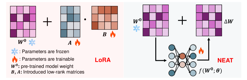
Figure 1: Framework of proposed Neat.

4 Methodology

4.1 Framework Overview

As shown in Fig. 1, the proposed Neat extends the incremental update mechanism of LoRA by introducing a non-linear weight adaptation approach for more expressive model updates. In LoRA, weight updates are achieved by decomposing adjustments into low-rank matrices $\bm{B}$ and $\bm{A}$, which are integrated into the pre-trained model weights $\bm{W}^{0}$. In contrast, Neat enhances this by replacing the static low-rank updates with a dynamic method. Specifically, Neat utilizes a neural network $f(\bm{W}^{0};\bm{\theta})$ that takes the pre-trained weights $\bm{W}^{0}$ as input and generates a non-linear update $\Delta\bm{W}$. This design allows Neat to capture more complex interactions and adapt more flexibly to a variety of tasks while maintaining parameter efficiency.

4.2 Motivation

In fully fine-tuning of pre-trained models, the weight update process is typically performed through iterative gradient descent:

$$\bm{W}^{0}_{t}=\bm{W}^{0}_{t-1}-\eta\nabla_{\bm{W}^{0}_{t-1}}\mathcal{L}$$ (3)

where $\bm{W}^{0}_{0}=\bm{W}^{0}$, $\eta$ is the learning rate, and $\bm{W}^{0}_{t}$ represents the weights after $t$ iterations. The cumulative change in the weights over time is represented as:

$$\Delta\bm{W}=\bm{W}^{0}_{t}-\bm{W}^{0}_{0}.$$ (4)

This weight change $\Delta\bm{W}$ can be interpreted as a function of the original pre-trained weights $\bm{W}^{0}$, capturing the model’s adaptation to the specific task during fine-tuning. Motivated by this observation, we propose to approximate $\Delta\bm{W}$ using a lightweight neural network that takes pre-trained model weight $\bm{W}^{0}$ as input and outputs the weight update directly. This approach leverages a nonlinear network to model the weight updating directly, which can capture more complex and richer transformation of the weights efficiently.

4.3 Nonlinear Parameter-efficient Adaptation

Similar to LoRA (Hu et al., 2021a), the proposed Neat also provides incremental update of pre-trained language models. However, Neat modifies the forward pass of the model by introducing a dynamic nonlinear weight transformation. Specifically, the model’s forward propagation is formulated as:

$$\bm{y}=(\bm{W}^{0}+f(\bm{W}^{0};\bm{\theta}))\bm{x},$$ (5)

where $\bm{x}$ and $\bm{y}$ are the input and output with respect to the current layer respectively and $f(\cdot;\bm{\theta}):\mathbb{R}^{d_{1}\times d_{2}}\to\mathbb{R}^{d_{1}\times d_{2}}$ is a nonlinear neural network parameterized by $\bm{\theta}$. The neural network $f(\bm{W}^{0};\bm{\theta})$ generates the weight update as a function of $\bm{W}^{0}$. In this formulation, the neural network $f(\bm{W}^{0};\bm{\theta})$ allows for dynamic, non-linear weight updates that can capture more complex interactions than the static low-rank approximation used in standard LoRA. To ensure the efficiency of the proposed Neat, the neural network $f(\bm{W}^{0};\bm{\theta})$ should be lightweight, i.e., the number of parameters of $f(\bm{W}^{0};\bm{\theta})$ is much smaller than that of original pre-trained weight $\bm{W}^{0}$. Therefore, we design the $f(\bm{W}^{0};\bm{\theta})$ as a neural network with bottleneck layers. For example, a simple case is $f(\bm{W}^{0};\bm{\theta})=\sigma(\bm{W}^{0}\bm{\Theta}_{1})\bm{\Theta}_{2}$, where $\bm{\theta}=(\bm{\Theta}_{1},\bm{\Theta}_{2})\in\mathbb{R}^{d_{2}\times r}\times\mathbb{R}^{r\times d_{2}}$ with $r\ll\min(d_{1},d_{2})$, and $\sigma(\cdot)$ is the activation function like ReLU (Glorot et al., 2011). We can also increase the layers or add activation function for the output of $f(\bm{W}^{0};\bm{\theta})$ to enhance the model expressiveness.

During fine-tuning, the optimization objective is to minimize the task-specific loss function, which can be represented as

$$\min_{\bm{\theta}}\mathcal{L}(\mathcal{D}_{\text{train}};\bm{W}^{0}+f(\bm{W}^{0};\bm{\theta})),$$ (6)

where the original pre-trained weight $\bm{W}^{0}$ is frozen, and only the parameters $\theta$ of the neural network $f(\bm{W}^{0};\bm{\theta})$ are updated.

5 Theoretical Analysis

In this section, we provide a theoretical analysis of Neat under ReLU activation. We show that Neat can achieve the same or greater expressivity than LoRA with fewer parameters under certain conditions. Consider a design of shallow neural network $f(\bm{W}^{0};\bm{\theta})=\sigma(\bm{W}^{0}\bm{\Theta}_{1})\bm{\Theta}_{2}$ as in Section 4.3.

Proposition 5.1.

Let $\sigma$ be a ReLU activation function. Let $\bm{U}\in\mathbb{R}^{d_{1}\times\operatorname{rank}(\bm{W}^{0})}$ be the left singular vectors of $\bm{W}^{0}$. Suppose that the loss function is invariant under the the projection of the weight matrix to the left singular space of $\bm{W}^{0}$, i.e., $\mathcal{L}(\mathcal{D}_{\text{train}};\bm{W})=\mathcal{L}(\mathcal{D}_{\text{train}};\bm{U}\bm{U}^{\top}\bm{W})$ for any $\bm{W}\in\mathbb{R}^{d_{1}\times d_{2}}$. Then, for any $r\geq 1$,

$$\min_{\begin{subarray}{c}\bm{\Theta}_{1}\in\mathbb{R}^{d_{2}\times 2r},\\ \bm{\Theta}_{2}\in\mathbb{R}^{2r\times d_{2}}\end{subarray}}\mathcal{L}(\mathcal{D}_{\text{train}};\bm{W}^{0}+f(\bm{W}^{0};(\bm{\Theta}_{1},\bm{\Theta}_{2}))) \leq\min_{\begin{subarray}{c}\bm{A}\in\mathbb{R}^{d_{1}\times r},\\ \bm{B}\in\mathbb{R}^{r\times d_{2}}\end{subarray}}\mathcal{L}(\mathcal{D}_{\text{train}};\bm{W}^{0}+\bm{A}\bm{B})$$

$$\leq\min_{\begin{subarray}{c}\bm{\Theta}_{1}\in\mathbb{R}^{d_{2}\times r},\\ \bm{\Theta}_{2}\in\mathbb{R}^{r\times d_{2}}\end{subarray}}\mathcal{L}(\mathcal{D}_{\text{train}};\bm{W}^{0}+f(\bm{W}^{0};(\bm{\Theta}_{1},\bm{\Theta}_{2}))).$$

Proposition 5.1 demonstrates that the minimum attainable loss using rank-$r$ LoRA can also be achieved by Neat with $2r$ hidden units, provided the invariance assumption holds. This suggests that Neat with $O(rd_{2})$ parameters maintains or surpasses the expressivity of LoRA with $r(d_{1}+d_{2})$ parameters. Since $d_{2}$ can be much smaller than $d_{1}$, this demonstrates a possibly significant improvement in parameter efficiency. The added expressivity can also improve sample efficiency by allowing the model to learn more detailed representations with the same or fewer data points.

The invariance assumption in Proposition 5.1 asserts that the model’s performance depends solely on the projection of the weight matrix onto the left singular space of $\bm{W}^{0}$. Given that we fine-tune a pre-trained model, the upper layers are expected to capture the task-relevant feature space, which is effectively described by the left singular space of $\bm{W}^{0}$. Since the upper layers primarily rely on this pre-trained feature space, the assumption is reasonable in practice. The principal directions of the pre-trained weight matrix, represented by its singular vectors, encode most of the useful features for downstream tasks, making the loss largely invariant to changes outside this subspace. The proof is available in Section A.1.

If we consider a sinusoid activation function $\sigma_{\textnormal{p}}(x)=\sin(2\pi x)$, we can show a stronger result without invariance assumption that Neat has expressivity (almost) greater than or equal to a LoRA with more parameters. We defer the result to the Appendix A.2.

6 Experiment

In the experiments, we evaluate the proposed Neat and answer the following questions:

1. How does Neat compare to state-of-the-art PEFT methods on NLP tasks?

2. How does Neat compare to state-of-the-art PEFT methods on vision tasks?

3. How does the performance of Neat vary with different fine-tuned modules, depths of the lightweight neural network, or non-linear activation functions?

6.1 Datasets and Experiment Settings

6.1.1 Datasets

We conduct experiments on four different benchmarks:

• Commonsense Reasoning, including BoolQ (Clark et al., 2019), PIQA (Bisk et al., 2020), SocialIQA (Sap et al., 2019), HellaSwag (Zellers et al., 2019), WinoGrande (Sakaguchi et al., 2019), ARC-e, ARC-c (Clark et al., 2018) and OpenBookQA (Mihaylov et al., 2018) datasets, is formulated as multiple-choice problems. Following Wang et al. (2024c), we finetune LLaMA2-7B (Touvron et al., 2023a) and LLaMA3-8B (AI@Meta, 2024) on Commonsense170K (Hu et al., 2023) dataset which is a combined training dataset of these tasks, and evaluate the Accuracy on each test set.

• Arithmetic Understanding consists of two math reasoning datasets: GSM8K (Cobbe et al., 2021) and MATH (Hendrycks et al., 2021). We finetune LLaMA2-7B (Touvron et al., 2023a) on MetaMath (Yu et al., 2023) dataset following Wang et al. (2024c). Models need to generate correct answers, and accuracy is used as the evaluation metric.

• Natural Language Understanding consists of eight datasets from the GLUE benchmark (Wang et al., 2018). We follow the evaluation metrics and setups from Gao et al. (2024); Wu et al. (2024a).

• Image Classification consists of eight datasets: OxfordPets (Parkhi et al., 2012), CIFAR10 (Krizhevsky, 2009), DTD (Cimpoi et al., 2014), EuroSAT (Helber et al., 2019), RESISC45 (Cheng et al., 2017), StanfordCars (Krause et al., 2013), FGVC (Maji et al., 2013) and CIFAR100 (Krizhevsky, 2009) following Gao et al. (2024). The first five datasets have small label spaces, while the last three have large label spaces.

Further details on the datasets and hyper-parameters are provided in Appendix D and Appendix C respectively.

6.1.2 Baselines

Our baselines are constructed on a task basis. Specifically, for each task, the proposed Neat is compared with representative baselines from the corresponding domain, as listed below.

• For both Commonsense Reasoning and Arithmetic Understanding, following Wang et al. (2024c), LoRA (Hu et al., 2021a), PiSSA (Meng et al., 2024) and MiLoRA (Wang et al., 2024c) are employed as baselines. Neat is applied to query, key, value, MLP up and MLP down layers.

• For Natural Language Understanding, we follow the setup from prior works (Gao et al., 2024; Wu et al., 2024a) that evaluate various representative PEFT methods, including LoRA (Hu et al., 2021a), Adapter Houlsby et al. (2019), BitFit (Zaken et al., 2021), RED (Wu et al., 2024b), DoRA (Liu et al., 2024), ReFT Wu et al. (2024a), and FourierFT (Gao et al., 2024).

• For Image Classification, we follow the setting of Gao et al. (2024) and take linear probing (LP), LoRA (Hu et al., 2021a) and FourierFT (Gao et al., 2024) as baselines. Neat is applied to the query and value layers.

6.2 Performance Comparison

6.2.1 Commonsense Reasoning

In this section, we present experiments on eight commonsense reasoning datasets to address RQ1, shown in Table LABEL:tab:commonsense. We compare the performance of three state-of-the-art baselines with the proposed Neat across eight different datasets. Neat consistently outperforms all baselines, achieving the highest accuracy on all tasks. Specifically, Neat surpasses LoRA, PiSSA, and MiLoRA in terms of average accuracy by 4.6%, 10%, and 2.5%, respectively, using LLaMA2-7B as the backbone. Furthermore, when using LLaMA3-8B as the backbone, Neat demonstrates average improvements of 4.9%, 11.8%, and 2.9% over LoRA, PiSSA, and MiLoRA, respectively. These results highlight the effectiveness and superiority of Neat as a PEFT method.

6.2.2 Arithmetic Reasoning

In this section, we present experiments on two arithmetic reasoning tasks, as shown in Table 2, to address RQ1. According to the table, full fine-tuning (FFT) achieves highest accuracy across the two datasets. However, the performance gap between the proposed Neat and FFT is quite small, despite Neat using significantly fewer trainable parameters. Moreover, compared to state-of-the-art PEFT baselines, the proposed Neat achieves substantial performance improvements. In terms of average accuracy, Neat demonstrates improvements of 7.5%, 12.4%, and 2.4% over LoRA, PiSSA, and MiLoRA, respectively. These results on arithmetic reasoning tasks suggest that Neat is a highly effective and efficient fine-tuning method for complex reasoning tasks.

Table 1: Accuracy comparison of LLaMA 2-7B (Touvron et al., 2023b) and LLaMA 3-8B (Dubey et al., 2024) against PEFT baselines on eight commonsense reasoning datasets. Results marked with “⁺” are taken from (Liu et al., 2024). Results marked with “^*” are taken from (Wang et al., 2024c). The highest accuracy of methods per category are in bold. “AVG” means the average accuracy of all datasets.

Model PEFT Accuracy ($\uparrow$) BoolQ PIQA SIQA HellaSwag WinoGrande ARC-e ARC-c OBQA AVG LLaMA2-7B LoRA⁺ 69.8 79.9 79.5 83.6 82.6 79.8 64.7 81.0 77.6 PiSSA^* 67.6 78.1 78.4 76.6 78.0 75.8 60.2 75.6 73.8 MiLoRA^* 67.6 83.8 80.1 88.2 82.0 82.8 68.8 80.6 79.2 Neat 71.7 83.9 80.2 88.9 84.3 86.3 71.4 83.0 81.2 LLaMA3-8B LoRA⁺ 70.8 85.2 79.9 91.7 84.3 84.2 71.2 79.0 80.8 PiSSA^* 67.1 81.1 77.2 83.6 78.9 77.7 63.2 74.6 75.4 MiLoRA^* 68.8 86.7 77.2 92.9 85.6 86.8 75.5 81.8 81.9 Neat 71.9 86.7 80.9 94.1 86.7 90.9 78.7 84.4 84.3

Table 2: Accuracy comparison of LLaMA 2-7B against PEFT baselines on two arithmetic reasoning datasets. Results marked with “⁺” are taken from (Yu et al., 2023). Results marked with “^*” are taken from (Wang et al., 2024c). The highest accuracy of methods per category are in bold. “AVG” means the average accuracy of all datasets.

Method	GSM8K	MATH	AVG
FFT +	66.50	19.80	43.20
LoRA*	60.58	16.88	38.73
PiSSA*	58.23	15.84	37.04
MiLoRA*	63.53	17.76	40.65
Neat	65.05	18.22	41.64

6.2.3 Natural Language Understanding

We conduct experiments on the GLUE to answer RQ1. The model performance is shown in Table 3. According to Table 3, the proposed Neat significantly outperforms state-of-the-art PEFT methods. Specifically, Neat-S, which uses a similar number of trainable parameters as FourierFT (Gao et al., 2024), DiReFT (Wu et al., 2024a), and LoReFT (Wu et al., 2024a), surpasses all PEFT baselines and experiences only a small performance drop (0.2%) compared to FFT. Additionally, Neat-L exceeds the performance of all baselines, including FFT, with the same number of trainable parameters as LoRA. These results demonstrate that the proposed Neat exhibits excellent generalization ability while maintaining high efficiency.

Table 3: Accuracy comparison of RoBERTa-base against PEFT baselines on the GLUE benchmark. Baseline results with “*” are taken from Wu et al. (2024b). The highest accuracy of methods per category are in bold. “AVG” means the average accuracy of all datasets. Neat-S refers to applying Neat only to the layers starting from the 4th layer, with the hidden layer dimension of the neural network set to 1. This configuration matches the parameter count of FourierFT. In contrast, Neat-L applies Neat to all layers, with the hidden layer dimension set to 8, aligning the parameter budget with LoRA.

PEFT Params (%) Accuracy ($\uparrow$) MNLI SST-2 MRPC CoLA QNLI QQP RTE STS-B AVG FFT 100% 87.3 94.4 87.9 62.4 92.5 91.7 78.3 90.6 85.6 Adapter^∗ 0.318% 87.0 93.3 88.4 60.9 92.5 90.5 76.5 90.5 85.0 LoRA^∗ 0.239% 86.6 93.9 88.7 59.7 92.6 90.4 75.3 90.3 84.7 Adapter^FNN∗ 0.239% 87.1 93.0 88.8 58.5 92.0 90.2 77.7 90.4 84.7 BitFit^∗ 0.080% 84.7 94.0 88.0 54.0 91.0 87.3 69.8 89.5 82.3 RED^∗ 0.016% 83.9 93.9 89.2 61.0 90.7 87.2 78.0 90.4 84.3 FourierFT 0.019% 84.7 94.2 90.0 63.8 92.2 88.0 79.1 90.8 85.3 DiReFT^∗ 0.015% 82.5 92.6 88.3 58.6 91.3 86.4 76.4 89.3 83.2 LoReFT^∗ 0.015% 83.1 93.4 89.2 60.4 91.2 87.4 79.0 90.0 84.2 Neat-S 0.019% 84.9 94.3 90.2 64.6 92.0 88.3 78.3 90.5 85.4 Neat-L 0.239% 86.6 94.6 90.0 64.4 92.7 89.7 78.7 90.9 86.0

Table 4: Accuracy comparison of ViT-base (Dosovitskiy et al., 2020b) against PEFT baselines on the image classification benchmark. The reported accuracy (%) is obtained after 10 epochs. The highest accuracy of methods per category are in bold. “AVG” means the average accuracy of all datasets. Results marked with “^∗” are taken from Gao et al. (2024).

Method	Params (M)	OxfordPets	StanfordCars	CIFAR10	DTD	EuroSAT	FGVC	RESISC45	CIFAR100	AVG
FFT∗	85.8M	93.14	79.78	98.92	77.68	99.05	54.84	96.13	92.38	86.49
LP∗	-	90.28	25.76	96.41	69.77	88.72	17.44	74.22	84.28	68.36
LoRA∗	581K	93.19	45.38	98.78	74.95	98.44	25.16	92.70	92.02	77.58
FourierFT∗	239K	93.05	56.36	98.69	77.30	98.78	32.44	94.26	91.45	80.29
Neat	258K	93.77	80.03	98.70	77.57	98.79	53.60	94.27	92.47	86.15

6.2.4 Image Classification

In this section, we present the experiments on image classification datasets to address RQ2, shown in Table 4. From the table, Neat significantly outperforms LoRA and FourierFT using the same number of trainable parameters. Specifically, Neat achieves performance improvements of 11.05%, 7.30%, and 26.02% compared to LoRA, FourierFT, and LP, respectively. Furthermore, compared to FFT (86.49%), the proposed Neat (86.15%) shows almost no performance drop while using only 0.3% of the trainable parameters required by FFT. This demonstrates that Neat exhibits exceptional adaptation capability not only on NLP tasks but also on vision tasks. Additionally, it verifies the effectiveness of the nonlinear adaptation used in Neat.

6.3 Sensitivity w.r.t. Fine-tuned Module

In this section, we present the results of applying Neat to various modules of ViT for image classification, addressing RQ3. The experimental results are shown in Fig. 3. We adjust the hidden layer dimension $r$ to maintain the same number of trainable parameters, ensuring a fair comparison. According to the figure, applying Neat to the QV layers yields results similar to applying Neat to both the QV and MLP layers. This indicates that Neat is robust across different fine-tuning module selections, potentially reducing the need for extensive hyper-parameter tuning when applying Neat to specific tasks.

6.4 Sensitivity w.r.t. Depth

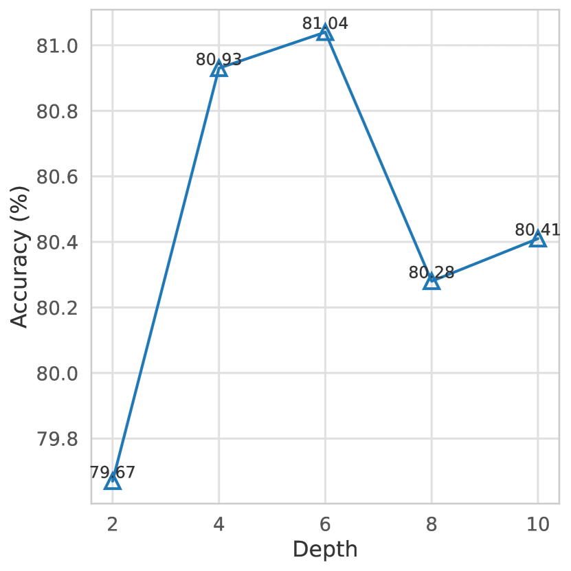
Figure 2: Accuracy on the StanfordCars dataset with varying depths of the neural network used in Neat. The depth here represents the total number of layers in the neural network. We choose depth equals to 2, 4, 6, 8, and 10 layers in the figure.

As the depth of a neural network increases, the model gains more nonlinearity, potentially making Neat more effective at capturing complex, non-linear patterns for weight updates. In this section, we present experiments with varying neural network depths in Neat on the StanfordCars dataset to address RQ3, as shown in Fig. 2. The architecture of the stacked layers used in Neat is shown in Fig. 4, with a detailed description provided in Appendix E. To ensure a fair comparison, we maintain consistent hyper-parameters across all configurations.

According to Fig. 2, increasing the network depth leads to better performance. Specifically, at a depth of 6 layers, the classification accuracy reaches 81.04%, marking a 1.7% improvement compared to using only 2 layers. When the depth is increased to 8 and 10 layers, the accuracy slightly decreases compared to the 6-layer model but remains higher than that of the 2-layer configuration. A possible explanation is that as depth increases—particularly at 10 layers—the training process becomes more challenging, possibly requiring more careful hyper-parameter tuning. It is also worth noting that, since the intermediate layers have much smaller dimensions ($\mathbb{R}^{r\times r}$ where $r$ is the hidden layer dimension) compared to the pre-trained model’s weight dimensions, the additional parameter overhead of stacking more hidden layers is negligible and does not affect the parameter efficiency of Neat. These results further demonstrate the effectiveness of introducing non-linear adaptation.

Figure 3: Accuracy of Neat with different targeted fine-tuning modules, including just QV layers and a combination of QV and MLP layers, on image classification datasets.

6.5 Sensitivity w.r.t. Different non-linear activations

Table 5: Accuracy of Neat with different nonlinear activation functions, i.e. ReLU and sinusoid functions, on image classification datasets. The highest accuracy of methods per category are in bold. “AVG” means the average accuracy of all datasets.

Method	OxfordPets	StanfordCars	CIFAR10	DTD	EuroSAT	FGVC	RESISC45	CIFAR100	AVG
ReLU	93.87	79.67	98.62	77.22	98.70	52.81	94.43	91.93	85.90
Sinusoid	93.51	79.95	98.88	79.08	98.74	53.47	93.62	92.25	86.19

A key innovation of Neat compared to LoRA and other PEFT methods, which rely solely on linear transformations for modeling weight updates, is the introduction of non-linear activations within the adaptation neural network. Since the choice of non-linear activations directly influences the learning process and the dynamics of weight updates, we investigate the impact of different non-linear activations on overall adaptation performance to address RQ3. Specifically, we compare Neat using $\sigma_{\textnormal{p}}(x)=\sin(2\pi x)$ as the non-linear activation function with Neat using ReLU, $\sigma_{\textnormal{p}}(x)=\max(0,x)$. The results are presented in Table 5. To ensure a fair comparison, the number of trainable parameters remains the same, and hyperparameters such as learning rate are optimized to maximize performance. The specific hyper-parameters for the sinusoidal non-linear activation setting are provided in Appendix C.1.

According to the table, using the sinusoidal non-linear activation generally results in better vision adaptation compared to using ReLU. Specifically, Neat with sinusoidal activation outperforms the ReLU-based Neat in 6 out of 8 tasks, particularly in DTD and FGVC. This observation aligns with our theoretical analysis in Section 5, which suggests that Neat with sinusoidal activation has equal or greater expressivity compared to using ReLU.

7 Conclusion

In this work, we propose Neat, a novel parameter-efficient fine-tuning (PEFT) method that introduces nonlinear transformations to enhance model adaptation while maintaining efficiency. By incorporating a lightweight neural network that models cumulative weight updates as functions of the pre-trained weights, Neat effectively captures complex, nonlinear structures in the weight space, allowing for more expressive and accurate adaptation to downstream tasks. Our theoretical analysis supports the efficacy of Neat, demonstrating that it can achieve greater or equivalent expressiveness compared to existing LoRA, a popular and state-of-the-art PEFT method, with fewer number of parameters. Through extensive experiments on four benchmarks encompassing over twenty datasets with various pre-trained backbones, Neat demonstrated superior performance on both NLP and vision tasks compared to existing state-of-the-art methods. Neat thus stands out as an effective solution for fine-tuning pre-trained models more adaptively and efficiently, which is crucial for resource-constrained environments.

Appendix

Appendix A Details of Theoretical Results

In this section, we provide the proof of Proposition 5.1 and introduce additional theoretical results when we assume sinusoid activation.

A.1 Proof of Proposition 5.1

The intuition behind the proof is that we can always restore an identity function using two ReLU activation functions, i.e., $x=\sigma(x)-\sigma(-x)$ for any $x\in\mathbb{R}$

Proof of Proposition 5.1.

We first show that

$$\min_{\bm{\Theta}_{1}\in\mathbb{R}^{d_{2}\times 2r},\bm{\Theta}_{2}\in\mathbb{R}^{2r\times d_{2}}}\mathcal{L}(\mathcal{D}_{\text{train}};\bm{W}^{0}+f(\bm{W}^{0};(\bm{\Theta}_{1},\bm{\Theta}_{2}))) \leq\min_{\bm{A}\in\mathbb{R}^{d_{1}\times r},\bm{B}\in\mathbb{R}^{r\times d_{2}}}\mathcal{L}(\mathcal{D}_{\text{train}};\bm{W}^{0}+\bm{A}\bm{B}).$$

Let $(\bm{A}^{*},\bm{B}^{*})=\operatorname*{arg\,min}_{\bm{A}\in\mathbb{R}^{d_{1}\times r},\bm{B}\in\mathbb{R}^{r\times d_{2}}}\mathcal{L}(\mathcal{D}_{\text{train}};\bm{W}^{0}+\bm{A}\bm{B})$. Take $\bm{\Theta}_{1}=[(\bm{W}^{0})^{\dagger}\bm{A}^{*};-(\bm{W}^{0})^{\dagger}\bm{A}^{*}]\in\mathbb{R}^{d_{2}\times 2r}$ and $\bm{\Theta}_{2}=[\bm{B}^{*\top};-\bm{B}^{*\top}]^{\top}\in\mathbb{R}^{2r\times d_{2}}$, where $(\bm{W}^{0})^{\dagger}\in\mathbb{R}^{d_{2}\times d_{1}}$ is the Moore-Penrose inverse of $\bm{W}^{0}$. Then, since $\sigma$ is a ReLU activation function,

$$f(\bm{W}^{0};(\bm{\Theta}_{1},\bm{\Theta}_{2})) =\sigma(\bm{W}^{0}\bm{\Theta}_{1})\bm{\Theta}_{2}$$

$$=\sigma(\bm{W}^{0}(\bm{W}^{0})^{\dagger}\bm{A}^{*})\bm{B}^{*}-\sigma(-\bm{W}^{0}(\bm{W}^{0})^{\dagger}\bm{A}^{*})\bm{B}^{*}$$

$$=\bm{W}^{0}(\bm{W}^{0})^{\dagger}\bm{A}^{*}\bm{B}^{*}.$$

where the last equality follows since $x$ is in the column space of $\bm{W}^{0}$. Note that $\bm{W}^{0}(\bm{W}^{0})^{\dagger}=\bm{U}\bm{U}^{\top}$ is the projection to the left singular space of $\bm{W}^{0}$. Hence

$$\mathcal{L}(\mathcal{D}_{\text{train}};\bm{W}^{0}+f(\bm{W}^{0};(\bm{\Theta}_{1},\bm{\Theta}_{2}))) =\mathcal{L}(\mathcal{D}_{\text{train}};\bm{U}\bm{U}^{\top}\bm{W}^{0}+\bm{U}\bm{U}^{\top}\bm{A}^{*}\bm{B}^{*})$$

$$=\mathcal{L}(\mathcal{D}_{\text{train}};\bm{W}^{0}+\bm{A}^{*}\bm{B}^{*}),$$

where the last equality follows from the invariance assumption.

To show the second inequality:

$$\min_{\bm{A}\in\mathbb{R}^{d_{1}\times r},\bm{B}\in\mathbb{R}^{r\times d_{2}}}\mathcal{L}(\mathcal{D}_{\text{train}};\bm{W}^{0}+\bm{A}\bm{B}) \leq\min_{\bm{\Theta}_{1}\in\mathbb{R}^{d_{2}\times r},\bm{\Theta}_{2}\in\mathbb{R}^{r\times d_{2}}}\mathcal{L}(\mathcal{D}_{\text{train}};\bm{W}^{0}+f(\bm{W}^{0};(\bm{\Theta}_{1},\bm{\Theta}_{2}))),$$

we can simply choose $\bm{A}=\sigma((\bm{W}^{0})^{\dagger}\bm{\Theta}_{1}^{*})\in\mathbb{R}^{d_{1}\times r}$ and $\bm{B}=\bm{\Theta}_{2}^{*}\in\mathbb{R}^{r\times d_{2}}$, where $(\bm{\Theta}_{1}^{*},\bm{\Theta}_{2}^{*})=\operatorname*{arg\,min}_{\bm{\Theta}_{1}\in\mathbb{R}^{d_{2}\times r},\bm{\Theta}_{2}\in\mathbb{R}^{r\times d_{1}}}\mathcal{L}(\mathcal{D}_{\text{train}};\bm{W}^{0}+f(\bm{W}^{0};(\bm{\Theta}_{1},\bm{\Theta}_{2})))$. This concludes the proof. ∎

A.2 Theoretical Analysis of Neat under sinusoid activation function

Here we consider a sinusoid activation function $\sigma_{\textnormal{p}}(x)=\sin(2\pi x)$ [Gashler and Ashmore, 2014] and design $f(\bm{W}^{0};\bm{\theta})=\sigma_{\textnormal{p}}(\bm{W}^{0}\bm{\Theta}_{1})\bm{\Theta}_{2}$ with $\bm{\theta}=(\bm{\Theta}_{1},\bm{\Theta}_{2})$. With this periodic activation function, we can show a stronger result that Neat has expressivity (almost) greater than or equal to a LoRA with more parameters when $d_{1}\gg d_{2}$.

Proposition A.1 (Expressivity of Neat with Sine Activation).

Suppose that there exists a row of $\bm{W}^{0}$, whose entries are linearly independent over the rationals. Then, for any $r>0$, $\bm{A}\in\mathbb{R}^{d_{1}\times r}$ and $\bm{B}\in\mathbb{R}^{r\times d_{2}}$, and $\epsilon>0$, there exists some $\bm{\Theta}_{1}^{*}\in\mathbb{R}^{d_{2}\times r}$ and $\bm{\Theta}_{2}^{*}\in\mathbb{R}^{r\times d_{2}}$ such that

$$\|\bm{A}\bm{B}-\sigma_{\textnormal{p}}(\bm{W}^{0}\bm{\Theta}_{1}^{*})\bm{\Theta}_{2}^{*}\|_{\textnormal{F}}\leq\epsilon.$$

Proposition A.1 shows that the class of updates $\Delta\bm{W}=\sigma_{\textnormal{p}}(\bm{W}^{0}\bm{\Theta}_{1})\bm{\Theta}_{2}$ by Neat with $2rd_{2}$ parameters is dense in the class of updates $\Delta\bm{W}=\bm{A}\bm{B}$ by LoRA with $r(d_{1}+d_{2})$ parameters. When $d_{2}\ll d_{2}$, this shows better parameter efficiency of Neat.

Examining the proof of Proposition A.1, it is straightforward to show that the result holds for any continuous and periodic activation function whose range contains an open interval centered at 0.

Proof.

This proof relies on Kronecker’s theorem (Theorem 7.9 in Apostol [1990]) from number theory, which shows that for all $j\in\mathbb{R}^{q}$, the fractional parts of $(ct_{1},ct_{2},\dots,ct_{q})^{\top}$ is dense in $[0,1]^{q}$ over $c\in\mathbb{R}$, as long as $t_{1},\dots,t_{q}$ are linearly independent over the rationals.

Let $\bm{w}_{j^{*}}$ be the $j^{*}$-th column of $\bm{W}^{0}$ whose entries are linearly independent over the rationals. Since $\bm{A}\bm{B}$ has a scale ambiguity, we can assume that $\bm{A}$ is a matrix whose entries are bounded by 1 without loss of generality. Write $\bm{A}=(\bm{a}_{1},\bm{a}_{2},\dots,\bm{a}_{r})$.

Take $\epsilon^{\prime}>0$ whose value will be determined later. From Kronecker’s theorem, for each $\bm{a}_{j}$ there exists some $c_{j}\in\mathbb{R}$ such that

$$\absolutevalue{\{c_{j}\bm{w}_{j^{*}}\}-\frac{\arcsin(\bm{a}_{j})}{2\pi}}\leq\epsilon^{\prime},$$

where $\{\bm{b}\}$ is a vector whose entries are the fractional part of the corresponding entry of $\bm{b}$, and $\arcsin$ is applied elementwisely.

Let $\bm{\Theta}_{1}^{*}=(c_{1}\bm{e}_{j^{*}},c_{2}\bm{e}_{j^{*}},\dots,c_{r}\bm{e}_{j^{*}})$, where $\bm{e}_{j^{*}}$ is the $j^{*}$-th standard basis vector in $\mathbb{R}^{d_{2}}$. Using the fact that $2\pi\{c_{j}\bm{w}_{j^{*}}\}=2\pi c_{j}\bm{w}_{j^{*}}\mod 2\pi$, we have

$$\norm{\sigma_{\textnormal{p}}(\bm{W}^{0}\bm{\Theta}_{1}^{*})-\bm{A}}_{\textnormal{F}}^{2} =\norm{\sigma_{\textnormal{p}}((c_{1}\bm{w}_{j^{*}},c_{2}\bm{w}_{j^{*}},\dots c_{r}\bm{w}_{j^{*}}))-\bm{A}}_{\textnormal{F}}^{2}$$ (7)

$$\leq\sum_{j}\norm{\sin(2\pi c_{j}\bm{w}_{j^{*}})-\bm{a}_{j}}^{2}\leq 4\pi^{2}r\epsilon^{\prime 2},$$ (8)

where the last inequality follows from equation 8 and the fact that $\sin(x)$ is Lipschitz continuous with Lipschitz constant 1. Hence by choosing $\bm{\Theta}_{2}^{*}\leftarrow\bm{B}$, we have

$$\norm{\bm{A}\bm{B}-\sigma_{\textnormal{p}}(\bm{W}^{0}\bm{\Theta}_{1}^{*})\bm{\Theta}_{2}^{*}}_{\textnormal{F}}^{2}\leq\norm{\bm{B}}^{2}\norm{\sigma_{\textnormal{p}}(\bm{W}^{0}\bm{\Theta}_{1}^{*})-\bm{A}}_{\textnormal{F}}^{2}\leq 4\pi^{2}\|\bm{B}\|^{2}r\epsilon^{\prime 2}.$$

Choose $\epsilon^{\prime}=\epsilon/(2\pi\sqrt{r}\|\bm{B}\|)$, then the proof is complete. ∎

Appendix B Additional Related Work

B.1 Additive PEFT Methods

Additive PEFT methods [Chronopoulou et al., 2023, Edalati et al., 2022, Lester et al., 2021, Wang et al., 2024a, Liu et al., 2022] introduces a small set of additional trainable parameters strategically placed within the model. One of the most prominent additive PEFT approaches is Adapter [Chronopoulou et al., 2023, Edalati et al., 2022, Zhao et al., 2022], which involves inserting small adapter layers between pre-trained weight blocks. Prompt Tuning [Wang et al., 2024a, Lester et al., 2021, Vu et al., 2021, Li and Liang, 2021] is another technique, where learnable vectors, or ”soft prompts,” are prepended to the input sequence without modifying the model’s weights. This method is particularly effective for large-scale models and has inspired variants such as Prefix Tuning [Li and Liang, 2021].

B.2 Selective PEFT Methods

Selective PEFT focuses on optimizing the fine-tuning process by selectively adjusting a subset of the model’s parameters rather than introducing additional ones. For instance, Diff Pruning [Guo et al., 2020] uses a learnable binary mask to select parameters for fine-tuning. Similarly, FishMask [Sung et al., 2021] and Fish-Dip [Das et al., 2023] leverage Fisher information to determine parameter importance and identify the most crucial ones for updates. Additionally, BitFit [Zaken et al., 2021] fine-tunes only the bias terms in the model, significantly reducing the number of trainable parameters.

B.3 Hybrid PEFT method

Hybrid PEFT methods aim to combine the strengths of various existing PEFT techniques to enhance model performance across diverse tasks. UniPELT [Mao et al., 2021] integrates LoRA, prefix-tuning, and adapters within each Transformer block, employing a gating mechanism to determine which module should be active during fine-tuning. S4 [Chen et al., 2023] further explores the design space by partitioning layers into groups and assigning different PEFT methods to each group. Additionally, NOAH [Zhang et al., 2022] and AUTOPEFT [Zhou et al., 2024] leverage neural architecture search (NAS) to automatically discover optimal combinations of PEFT techniques tailored to specific tasks.

Appendix C Hyperparameters

We provide the specific hyperparameters used in our experiments to ensure reproducibility. For most of our experiments, we use the standard implementation of Neat, which we refer to as vanilla Neat. The neural network architecture in vanilla Neat consists of only two layers: an input layer and an output layer. We selecte this approach because vanilla Neat offers the benefits of simplicity in implementation, a low parameter count, and sufficient adaptation power. Nonetheless, we dedicate Section 6.4 and Appendix E to exploring more complex adaptation networks and their effect on performance.

C.1 Image Classification

Hyperparameters for Neat in image classification are provided in Table 6. We tune the classification head and the backbone separately and provide detailed settings for each dataset. All weight decay values are not tuned and follow the settings from Gao et al. [2024]. The scaling factor $s$ is set to $1.0$. The hidden layer dimension $r$ for MHSA is set to 7 in the QV-setting, while both hidden layer dimensions for MHSA and MLP are set to 2 in the QV-MLP-setting described in Section 6.3. Additionally, specific hyper-parameters for the sinusoidal non-linear activation analysis are provided in Table 7.

Table 6: Hyperparameter of image classification for Neat.

Hyperparameter	OxfordPets	StanfordCars	CIFAR10	DTD	EuroSAT	FGVC	RESISC45	CIFAR100
Epochs	10
Optimizer	AdamW
LR Schedule	Linear
Weight Decay	8E-4	4E-5	9E-5	7E-5	3E-4	7E-5	3E-4	1E-4
QV
Learning Rate (Neat)	5E-3	1E-2	5E-3	1E-2	5E-3	1E-2	5E-3	5E-3
Learning Rate (Head)	5E-3	1E-2	5E-3	1E-2	5E-3	1E-2	1E-2	5E-3
QV-MLP
Learning Rate (Neat)	5E-3	5E-3	5E-3	1E-2	5E-3	5E-3	1E-2	5E-3
Learning Rate (Head)	5E-3	1E-2	5E-3	1E-2	5E-3	1E-2	1E-2	5E-3

Table 7: Hyperparameters for image classification with Neat using sinusoidal non-linear activation. The targeted modules are the same as the QV-setting (i.e., only adapting the query and value layers with a hidden layer dimension of 7).

Hyperparameter	OxfordPets	StanfordCars	CIFAR10	DTD	EuroSAT	FGVC	RESISC45	CIFAR100
Epochs	10
Optimizer	AdamW
LR Schedule	Linear
Weight Decay	8E-4	4E-5	9E-5	7E-5	3E-4	7E-5	3E-4	1E-4
Learning Rate (Neat)	5E-3	5E-3	1E-3	5E-3	1E-3	5E-3	5E-3	1E-3
Learning Rate (Head)	5E-3	1E-2	5E-3	1E-2	5E-3	1E-2	1E-2	5E-3

C.2 Natural Language Understanding

We provide used hyper-parameters for Neat in natural language understanding on the GLUE benchmark in Table 8 and Table 9. The learning rates for the head and the backbone are tuned separately. The scaling factor $s$ is searched in $\{0.01,0.1,1.0\}$. For reproducibility, we fix the seed as 0. The hidden layer dimension $r$ is set to 8 in Neat-L and 1 in Neat-S. More specifically, we apply Neat to all layers in RoBERTa-base for Neat-L, while only applying Neat to layers $\{4,5,6,7,8,9,10,11\}$ for Neat-S to reduce the number of trainable parameters. The seed is fixed for reproducibility.

Table 8: Hyperparameter of GLUE benchmark for Neat-L.

Hyperparameter	STS-B	RTE	MRPC	CoLA	SST-2	QNLI	MNLI	QQP
Optimizer	AdamW
LR Schedule	Linear
Learning Rate (Neat)	5E-3	5E-3	5E-3	1E-3	5E-3	1E-3	5E-3	5E-3
Learning Rate (Head)	5E-3	5E-3	5E-3	1E-3	5E-3	1E-3	5E-3	5E-3
Scaling	0.1	0.01	0.01	0.1	0.01	0.01	0.01	0.01
Max Seq. Len	512	512	512	512	512	512	512	512
Batch Size	64	32	64	64	32	32	32	64

Table 9: Hyperparameter of GLUE benchmark for Neat-S.

Hyperparameter	STS-B	RTE	MRPC	CoLA	SST-2	QNLI	MNLI	QQP
Optimizer	AdamW
LR Schedule	Linear
Learning Rate (Neat)	5E-3	1E-3	5E-3	5E-3	5E-3	1E-3	5E-3	1E-3
Learning Rate (Head)	1E-3	1E-3	5E-3	1E-3	5E-3	1E-3	5E-3	1E-3
Scaling	0.1	1.0	0.01	0.1	0.01	0.1	0.01	1.0
Max Seq. Len	512	512	512	512	512	512	512	512
Batch Size	64	32	64	64	32	32	32	64

C.3 Commonsense Reasoning

Table 10: Hyperparameter of commonsense reasoning for Neat.

Hyperparameter	Commonsense Reasoning
Hidden Layer Dimension	32
$\alpha$	32
Dropout	0.05
Optimizer	Adam W
Learning Rate	3e-4
Batch Size	16
Warmup Steps	100
Epochs	1

We provide hyperparameters settings of Neat for commonsense reasoning task in Table 10. We follow the hyperparameters settings in MiLoRA [Wang et al., 2024c]. We limit all samples to a maximum of 256 tokens. For evaluation, we set a maximum token number of 32.

C.4 Arithmetic Reasoning

Table 11: Hyperparameter of arithmetic reasoning for Neat.

Hyperparameter	Arithmetic Reasoning
Hidden Layer Dimension	64
$\alpha$	64
Dropout	0.05
Optimizer	Adam W
Learning Rate	3e-4
Batch Size	16
Warmup Steps	100
Epochs	3

We provide hyperparameters settings of Neat for arithmetic reasoning task in Table 11. We follow the hyper-parameters settings in MiLoRA [Wang et al., 2024c]. We limit all samples to a maximum of 2048 tokens. For evaluation, we set a maximum token number of 256 on GSM8K [Cobbe et al., 2021] dataset. On MATH [Hendrycks et al., 2021], we set the maximum new token to 512.

Appendix D Datasets

In this section, we provide a detailed description of the datasets used in our experiments.

D.1 Image Classification

For image classification, we provide detailed information about the used datasets in Table 12.

Table 12: Detailed information of image classification tasks.

Dataset	#Class	#Train	#Val	#Test	Rescaled resolution
OxfordPets	37	3,312	368	3,669	$224\times 224$
StandfordCars	196	7,329	815	8,041
CIFAR10	10	45,000	5,000	10,000
DTD	47	4,060	452	1,128
EuroSAT	10	16,200	5,400	5,400
FGVC	100	3,000	334	3,333
RESISC45	45	18,900	6,300	6,300
CIFAR100	100	45,000	5,000	10,000

D.2 Natural Language Understanding

The GLUE benchmark comprises 8 NLP datasets: MNLI, SST-2, MRPC, CoLA, QNLI, QQP, RTE, and STS-B, covering tasks such as inference, sentiment analysis, paraphrase detection, linguistic acceptability, question-answering, and textual similarity. We provide detailed information about them in Table 13.

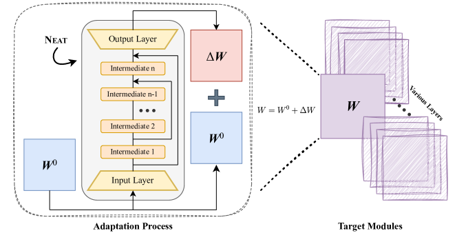
Figure 4: Implementation of introducing more depths to Neatt. We insert multiple intermediate layers into the layers from vanilla Neat, with non-linear activation in between. The depth is described as the number of layers in Neat, with vanilla Neat having a depth of 2 (i.e. the input and output layers).

Table 13: Detailed information of the GLUE benchmark. STS-B is a regression task, while all other tasks are either single-sentence or sentence-pair classification tasks.

Corpus	Task	Metrics	# Train	# Val	# Test	# Labels
Single-Sentence Tasks
CoLA	Acceptability	Matthews Corr.	8.55k	1.04k	1.06k	2
SST-2	Sentiment	Accuracy	67.3k	872	1.82k	2
Similarity and Paraphrase Tasks
MRPC	Paraphrase	Accuracy/F1	3.67k	408	1.73k	2
STS-B	Sentence similarity	Pearson/Spearman Corr.	5.75k	1.5k	1.38k	1
QQP	Paraphrase	Accuracy/F1	364k	40.4k	391k	2
Inference Tasks
MNLI	NLI	Accuracy	393k	19.65k	19.65k	3
QNLI	QA/NLI	Accuracy	105k	5.46k	5.46k	2
RTE	NLI	Accuracy	2.49k	277	3k	2

D.3 Commonsense Reasoning

Table 14: Detailed information of commonsense reasoning task.

Dataset	#Class	#Train	#Dev	#Test
BoolQ	Binary classification	9,427	3,270	3,245
PIQA	Binary classification	16,113	1,838	3,000
SIQA	Ternary classification	33,410	1,954	2,224
HellaSwag	Quaternary classification	39,905	10,042	10,003
WinoGrande	Binary classification	40,398	1,267	1,767
ARC-e	Quaternary classification	2,251	570	2,376
ARC-c	Quaternary classification	1,119	229	1,172
OBQA	Quaternary classification	4,957	500	500

For commonsense reasoning task, we use 8 datasets, including BoolQ, PIQA, SIQA, HellaSwag, WinoGrande, ARC-e, ARC-c and OBQA. The detailed information is provided in Table 14.

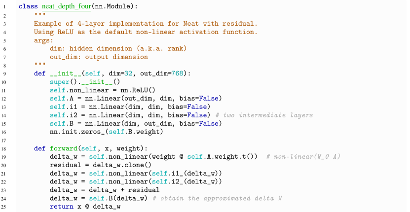
Figure 5: An example of the actual implementation applying 4 layers in Neat (depth = 4) with Pytorch.

D.4 Arithmetic Reasoning

Table 15: Detailed information of arithmetic reasoning task.

Dataset	#Train	#Dev	#Test
GSM8K	7,473	1,319	1,319
MATH	12,500	500	5,000

Detailed information for arithmetic reasoning task is provided in Table 15. GSM8K consists of high quality grade school math problems, typically free-form answers. MATH includes classifications from multiple mathematical domains, such as algebra, counting_and_probability, geometry, intermediate_algebra, number_theory, prealgebra and precalculus.

Appendix E Implementation of Introducing Depths to Neat

We provide a comprehensive explanation of our approach to increasing the depth of the adaptation neural network in Neat. As depicted in Fig. 4, we introduce multiple deeply stacked intermediate layers between the layers of the vanilla Neat. These intermediate layers are essentially small adapters with a minimal parameter count ($\mathbb{R}^{r\times r}$, where $r$ is the hidden layer dimension), and we retain non-linear activations between them, as proposed by Neat. The adaptation process begins by feeding the weight matrix $W^{0}$—the initialized value of the adaptation target $W$—into Neat’s input layer. After undergoing multiple non-linear transformations through the intermediate layers, the final layer projects $W^{0}$ back to its original shape, producing the adaptation result $\Delta W$. Throughout this process, the adaptation target remains fixed, while all the intermediate layers, as well as the input and output layers in Neat, are trainable parameters.

Furthermore, an implementation example of Neat with four layers using the PyTorch library is illustrated in Fig. 5. As previously mentioned, we apply non-linear activations (ReLU in this case) to model more complex transformations. The intermediate layers have the same shape, $\mathbb{R}^{r\times r}$, which adds minimal overhead compared to $A\in\mathbb{R}^{d_{2}\times r}$ and $B\in\mathbb{R}^{r\times d_{2}}$—the input and output layers, respectively, which are also present in the vanilla Neat. Since $d_{2}$ is typically in the range of hundreds to thousands, while $r$ is commonly set to 8, 16, or 32, the parameter efficiency of Neat with deeper layers remains comparable to that of vanilla Neat without the intermediate layers. As shown, we first transform $W^{0}$ into the desired adaptation result $\Delta W$ and subsequently use $\Delta W$ to perform the actual computation on the input data. The use of residuals is based on empirical observations, as incorporating residual connections in the adaptation process results in faster convergence, more stable loss curves, and significantly improved overall performance.

References

- Devlin [2018] Jacob Devlin. Bert: Pre-training of deep bidirectional transformers for language understanding. arXiv preprint arXiv:1810.04805, 2018.
- Liu [2019] Yinhan Liu. Roberta: A robustly optimized bert pretraining approach. arXiv preprint arXiv:1907.11692, 2019.
- Touvron et al. [2023a] Hugo Touvron, Louis Martin, Kevin Stone, Peter Albert, Amjad Almahairi, Yasmine Babaei, Nikolay Bashlykov, Soumya Batra, and et al. Llama 2: Open foundation and fine-tuned chat models. arXiv preprint arXiv:2307.09288, 2023a.
- AI@Meta [2024] AI@Meta. Llama 3 model card. 2024. URL https://github.com/meta-llama/llama3/blob/main/MODEL_CARD.md.
- Dosovitskiy et al. [2020a] Alexey Dosovitskiy, Lucas Beyer, Alexander Kolesnikov, Dirk Weissenborn, Xiaohua Zhai, Thomas Unterthiner, Mostafa Dehghani, Matthias Minderer, Georg Heigold, Sylvain Gelly, et al. An image is worth 16x16 words: Transformers for image recognition at scale. In International Conference on Learning Representations, 2020a.
- Qin et al. [2024] Ruiyang Qin, Dancheng Liu, Zheyu Yan, Zhaoxuan Tan, Zixuan Pan, Zhenge Jia, Meng Jiang, Ahmed Abbasi, Jinjun Xiong, and Yiyu Shi. Empirical guidelines for deploying llms onto resource-constrained edge devices. arXiv preprint arXiv:2406.03777, 2024.
- Ding et al. [2023] Ning Ding, Yujia Qin, Guang Yang, Fuchao Wei, Zonghan Yang, Yusheng Su, Shengding Hu, Yulin Chen, Chi-Min Chan, Weize Chen, et al. Parameter-efficient fine-tuning of large-scale pre-trained language models. Nature Machine Intelligence, 5(3):220–235, 2023.
- Han et al. [2024] Zeyu Han, Chao Gao, Jinyang Liu, Sai Qian Zhang, et al. Parameter-efficient fine-tuning for large models: A comprehensive survey. arXiv preprint arXiv:2403.14608, 2024.
- Lin et al. [2024] Ji Lin, Jiaming Tang, Haotian Tang, Shang Yang, Wei-Ming Chen, Wei-Chen Wang, Guangxuan Xiao, Xingyu Dang, Chuang Gan, and Song Han. Awq: Activation-aware weight quantization for on-device llm compression and acceleration. Proceedings of Machine Learning and Systems, 6:87–100, 2024.
- Hu et al. [2021a] Edward J Hu, Yelong Shen, Phillip Wallis, Zeyuan Allen-Zhu, Yuanzhi Li, Shean Wang, Lu Wang, and Weizhu Chen. Lora: Low-rank adaptation of large language models. arXiv preprint arXiv:2106.09685, 2021a.
- Liu et al. [2024] Shih-Yang Liu, Chien-Yi Wang, Hongxu Yin, Pavlo Molchanov, Yu-Chiang Frank Wang, Kwang-Ting Cheng, and Min-Hung Chen. DoRA: Weight-decomposed low-rank adaptation. arXiv:2402.09353, 2024. URL https://arxiv.org/abs/2402.09353.
- Song et al. [2024] Lin Song, Yukang Chen, Shuai Yang, Xiaohan Ding, Yixiao Ge, Ying-Cong Chen, and Ying Shan. Low-rank approximation for sparse attention in multi-modal llms. In Proceedings of the IEEE/CVF Conference on Computer Vision and Pattern Recognition, pages 13763–13773, 2024.
- Büyükakyüz [2024] Kerim Büyükakyüz. Olora: Orthonormal low-rank adaptation of large language models. arXiv preprint arXiv:2406.01775, 2024.
- Zhao et al. [2024] Jiawei Zhao, Zhenyu Zhang, Beidi Chen, Zhangyang Wang, Anima Anandkumar, and Yuandong Tian. Galore: Memory-efficient llm training by gradient low-rank projection. arXiv preprint arXiv:2403.03507, 2024.
- Pan et al. [2024] Rui Pan, Xiang Liu, Shizhe Diao, Renjie Pi, Jipeng Zhang, Chi Han, and Tong Zhang. Lisa: Layerwise importance sampling for memory-efficient large language model fine-tuning. arXiv preprint arXiv:2403.17919, 2024.
- Chronopoulou et al. [2023] Alexandra Chronopoulou, Matthew E Peters, Alexander Fraser, and Jesse Dodge. Adaptersoup: Weight averaging to improve generalization of pretrained language models. arXiv preprint arXiv:2302.07027, 2023.
- Edalati et al. [2022] Ali Edalati, Marzieh Tahaei, Ivan Kobyzev, Vahid Partovi Nia, James J Clark, and Mehdi Rezagholizadeh. Krona: Parameter efficient tuning with kronecker adapter. arXiv preprint arXiv:2212.10650, 2022.
- Lester et al. [2021] Brian Lester, Rami Al-Rfou, and Noah Constant. The power of scale for parameter-efficient prompt tuning. arXiv preprint arXiv:2104.08691, 2021.
- Wang et al. [2024a] Yihan Wang, Jatin Chauhan, Wei Wang, and Cho-Jui Hsieh. Universality and limitations of prompt tuning. Advances in Neural Information Processing Systems, 36, 2024a.
- Liu et al. [2022] Haokun Liu, Derek Tam, Mohammed Muqeeth, Jay Mohta, Tenghao Huang, Mohit Bansal, and Colin A Raffel. Few-shot parameter-efficient fine-tuning is better and cheaper than in-context learning. Advances in Neural Information Processing Systems, 35:1950–1965, 2022.
- Guo et al. [2020] Demi Guo, Alexander M Rush, and Yoon Kim. Parameter-efficient transfer learning with diff pruning. arXiv preprint arXiv:2012.07463, 2020.
- Das et al. [2023] Sarkar Snigdha Sarathi Das, Ranran Haoran Zhang, Peng Shi, Wenpeng Yin, and Rui Zhang. Unified low-resource sequence labeling by sample-aware dynamic sparse finetuning. arXiv preprint arXiv:2311.03748, 2023.
- Sung et al. [2021] Yi-Lin Sung, Varun Nair, and Colin A Raffel. Training neural networks with fixed sparse masks. Advances in Neural Information Processing Systems, 34:24193–24205, 2021.
- Ansell et al. [2021] Alan Ansell, Edoardo Maria Ponti, Anna Korhonen, and Ivan Vulić. Composable sparse fine-tuning for cross-lingual transfer. arXiv preprint arXiv:2110.07560, 2021.
- Zaken et al. [2021] Elad Ben Zaken, Shauli Ravfogel, and Yoav Goldberg. Bitfit: Simple parameter-efficient fine-tuning for transformer-based masked language-models. arXiv preprint arXiv:2106.10199, 2021.
- Vucetic et al. [2022] Danilo Vucetic, Mohammadreza Tayaranian, Maryam Ziaeefard, James J Clark, Brett H Meyer, and Warren J Gross. Efficient fine-tuning of bert models on the edge. In 2022 IEEE International Symposium on Circuits and Systems (ISCAS), pages 1838–1842, 2022.
- Hu et al. [2021b] Edward J Hu, Yelong Shen, Phillip Wallis, Zeyuan Allen-Zhu, Yuanzhi Li, Shean Wang, Lu Wang, and Weizhu Chen. Lora: Low-rank adaptation of large language models. arXiv preprint arXiv:2106.09685, 2021b.
- Valipour et al. [2022] Mojtaba Valipour, Mehdi Rezagholizadeh, Ivan Kobyzev, and Ali Ghodsi. Dylora: Parameter efficient tuning of pre-trained models using dynamic search-free low-rank adaptation. arXiv preprint arXiv:2210.07558, 2022.
- Zhang et al. [2023] Qingru Zhang, Minshuo Chen, Alexander Bukharin, Nikos Karampatziakis, Pengcheng He, Yu Cheng, Weizhu Chen, and Tuo Zhao. Adalora: Adaptive budget allocation for parameter-efficient fine-tuning. arXiv preprint arXiv:2303.10512, 2023.
- Karimi Mahabadi et al. [2021] Rabeeh Karimi Mahabadi, James Henderson, and Sebastian Ruder. Compacter: Efficient low-rank hypercomplex adapter layers. Advances in Neural Information Processing Systems, 34:1022–1035, 2021.
- Kopiczko et al. [2023] Dawid Jan Kopiczko, Tijmen Blankevoort, and Yuki Markus Asano. Vera: Vector-based random matrix adaptation. arXiv preprint arXiv:2310.11454, 2023.
- Mao et al. [2021] Yuning Mao, Lambert Mathias, Rui Hou, Amjad Almahairi, Hao Ma, Jiawei Han, Wen-tau Yih, and Madian Khabsa. Unipelt: A unified framework for parameter-efficient language model tuning. arXiv preprint arXiv:2110.07577, 2021.
- Chen et al. [2023] Jiaao Chen, Aston Zhang, Xingjian Shi, Mu Li, Alex Smola, and Diyi Yang. Parameter-efficient fine-tuning design spaces. arXiv preprint arXiv:2301.01821, 2023.
- He et al. [2021] Junxian He, Chunting Zhou, Xuezhe Ma, Taylor Berg-Kirkpatrick, and Graham Neubig. Towards a unified view of parameter-efficient transfer learning. arXiv preprint arXiv:2110.04366, 2021.
- Zhang et al. [2022] Yuanhan Zhang, Kaiyang Zhou, and Ziwei Liu. Neural prompt search. arXiv preprint arXiv:2206.04673, 2022.
- Zhou et al. [2024] Han Zhou, Xingchen Wan, Ivan Vulić, and Anna Korhonen. Autopeft: Automatic configuration search for parameter-efficient fine-tuning. Transactions of the Association for Computational Linguistics, 12:525–542, 2024.
- Wang et al. [2024b] Haoyu Wang, Tianci Liu, Tuo Zhao, and Jing Gao. Roselora: Row and column-wise sparse low-rank adaptation of pre-trained language model for knowledge editing and fine-tuning. arXiv preprint arXiv:2406.10777, 2024b.
- [38] Ziqi Gao, Qichao Wang, Aochuan Chen, Zijing Liu, Bingzhe Wu, Liang Chen, and Jia Li. Parameter-efficient fine-tuning with discrete fourier transform. In Forty-first International Conference on Machine Learning.
- Meng et al. [2024] Fanxu Meng, Zhaohui Wang, and Muhan Zhang. Pissa: Principal singular values and singular vectors adaptation of large language models. arXiv preprint arXiv:2404.02948, 2024.
- Wang et al. [2024c] Hanqing Wang, Zeguan Xiao, Yixia Li, Shuo Wang, Guanhua Chen, and Yun Chen. Milora: Harnessing minor singular components for parameter-efficient llm finetuning. arXiv preprint arXiv:2406.09044, 2024c.
- Glorot et al. [2011] Xavier Glorot, Antoine Bordes, and Yoshua Bengio. Deep sparse rectifier neural networks. In Proceedings of the fourteenth international conference on artificial intelligence and statistics, pages 315–323. JMLR Workshop and Conference Proceedings, 2011.
- Clark et al. [2019] Christopher Clark, Kenton Lee, Ming-Wei Chang, Tom Kwiatkowski, Michael Collins, and Kristina Toutanova. Boolq: Exploring the surprising difficulty of natural yes/no questions. arXiv preprint arXiv:1905.10044, 2019.
- Bisk et al. [2020] Yonatan Bisk, Rowan Zellers, Ronan Le Bras, Jianfeng Gao, and Yejin Choi. Piqa: Reasoning about physical commonsense in natural language. arXiv preprint arXiv:1911.11641, 2020.
- Sap et al. [2019] Maarten Sap, Hannah Rashkin, Derek Chen, Ronan LeBras, and Yejin Choi. Socialiqa: Commonsense reasoning about social interactions. arXiv preprint arXiv:1904.09728, 2019.
- Zellers et al. [2019] Rowan Zellers, Ari Holtzman, Yonatan Bisk, Ali Farhadi, and Yejin Choi. Hellaswag: Can a machine really finish your sentence? arXiv preprint arXiv:1905.07830, 2019.
- Sakaguchi et al. [2019] Keisuke Sakaguchi, Ronan Le Bras, Chandra Bhagavatula, and Yejin Choi. Winogrande: An adversarial winograd schema challenge at scale. arXiv preprint arXiv:1907.10641, 2019.
- Clark et al. [2018] Peter Clark, Isaac Cowhey, Oren Etzioni, Tushar Khot, Ashish Sabharwal, Carissa Schoenick, and Oyvind Tafjord. Think you have solved question answering? try arc, the ai2 reasoning challenge. arXiv preprint arXiv:1803.05457, 2018.
- Mihaylov et al. [2018] Todor Mihaylov, Peter Clark, Tushar Khot, and Ashish Sabharwal. Can a suit of armor conduct electricity? a new dataset for open book question answering. arXiv preprint arXiv:1809.02789, 2018.
- Hu et al. [2023] Zhiqiang Hu, Lei Wang, Yihuai Lan, Wanyu Xu, Ee-Peng Lim, Lidong Bing, Xing Xu, Soujanya Poria, and Roy Lee. Llm-adapters: An adapter family for parameter-efficient fine-tuning of large language models. arXiv preprint arXiv:2304.01933, 2023.
- Cobbe et al. [2021] Karl Cobbe, Vineet Kosaraju, Mohammad Bavarian, Mark Chen, Heewoo Jun, Lukasz Kaiser, Matthias Plappert, Jerry Tworek, Jacob Hilton, Reiichiro Nakano, Christopher Hesse, and John Schulman. Training verifiers to solve math word problems. arXiv preprint arXiv:2110.14168, 2021.
- Hendrycks et al. [2021] Dan Hendrycks, Collin Burns, Saurav Kadavath, Akul Arora, Steven Basart, Eric Tang, Dawn Song, and Jacob Steinhardt. Measuring mathematical problem solving with the math dataset. arXiv preprint arXiv:2103.03874, 2021.
- Yu et al. [2023] Longhui Yu, Weisen Jiang, Han Shi, Jincheng Yu, Zhengying Liu, Yu Zhang, James T. Kwok, Zhenguo Li, Adrian Weller, and Weiyang Liu. Metamath: Bootstrap your own mathematical questions for large language models. arXiv preprint arXiv:2309.12284, 2023.
- Wang et al. [2018] Alex Wang, Amanpreet Singh, Julian Michael, Felix Hill, Omer Levy, and Samuel R Bowman. Glue: A multi-task benchmark and analysis platform for natural language understanding. arXiv preprint arXiv:1804.07461, 2018.
- Gao et al. [2024] Ziqi Gao, Qichao Wang, Aochuan Chen, Zijing Liu, Bingzhe Wu, Liang Chen, and Jia Li. Parameter-efficient fine-tuning with discrete fourier transform. arXiv preprint arXiv:2405.03003, 2024.
- Wu et al. [2024a] Zhengxuan Wu, Aryaman Arora, Zheng Wang, Atticus Geiger, Dan Jurafsky, Christopher D. Manning, and Christopher Potts. ReFT: Representation finetuning for language models. 2024a. URL arxiv.org/abs/2404.03592.
- Parkhi et al. [2012] Omkar M Parkhi, Andrea Vedaldi, Andrew Zisserman, and CV Jawahar. Cats and dogs. In 2012 IEEE conference on computer vision and pattern recognition, pages 3498–3505. IEEE, 2012.
- Krizhevsky [2009] A Krizhevsky. Learning multiple layers of features from tiny images. Master’s thesis, University of Tront, 2009.
- Cimpoi et al. [2014] Mircea Cimpoi, Subhransu Maji, Iasonas Kokkinos, Sammy Mohamed, and Andrea Vedaldi. Describing textures in the wild. In Proceedings of the IEEE conference on computer vision and pattern recognition, pages 3606–3613, 2014.
- Helber et al. [2019] Patrick Helber, Benjamin Bischke, Andreas Dengel, and Damian Borth. Eurosat: A novel dataset and deep learning benchmark for land use and land cover classification. IEEE Journal of Selected Topics in Applied Earth Observations and Remote Sensing, 12(7):2217–2226, 2019.
- Cheng et al. [2017] Gong Cheng, Junwei Han, and Xiaoqiang Lu. Remote sensing image scene classification: Benchmark and state of the art. Proceedings of the IEEE, 105(10):1865–1883, 2017.
- Krause et al. [2013] Jonathan Krause, Michael Stark, Jia Deng, and Li Fei-Fei. 3d object representations for fine-grained categorization. In Proceedings of the IEEE international conference on computer vision workshops, pages 554–561, 2013.
- Maji et al. [2013] Subhransu Maji, Esa Rahtu, Juho Kannala, Matthew Blaschko, and Andrea Vedaldi. Fine-grained visual classification of aircraft. arXiv preprint arXiv:1306.5151, 2013.
- Houlsby et al. [2019] Neil Houlsby, Andrei Giurgiu, Stanislaw Jastrzebski, Bruna Morrone, Quentin De Laroussilhe, Andrea Gesmundo, Mona Attariyan, and Sylvain Gelly. Parameter-efficient transfer learning for nlp. In International conference on machine learning, pages 2790–2799. PMLR, 2019.
- Wu et al. [2024b] Muling Wu, Wenhao Liu, Xiaohua Wang, Tianlong Li, Changze Lv, Zixuan Ling, Jianhao Zhu, Cenyuan Zhang, Xiaoqing Zheng, and Xuanjing Huang. Advancing parameter efficiency in fine-tuning via representation editing. arXiv:2402.15179, 2024b. URL https://arxiv.org/abs/2402.15179.
- Touvron et al. [2023b] Hugo Touvron, Louis Martin, Kevin Stone, Peter Albert, Amjad Almahairi, Yasmine Babaei, Nikolay Bashlykov, Soumya Batra, Prajjwal Bhargava, Shruti Bhosale, et al. Llama 2: Open foundation and fine-tuned chat models. arXiv preprint arXiv:2307.09288, 2023b.
- Dubey et al. [2024] Abhimanyu Dubey, Abhinav Jauhri, Abhinav Pandey, Abhishek Kadian, Ahmad Al-Dahle, Aiesha Letman, Akhil Mathur, Alan Schelten, Amy Yang, Angela Fan, et al. The llama 3 herd of models. arXiv preprint arXiv:2407.21783, 2024.
- Dosovitskiy et al. [2020b] Alexey Dosovitskiy, Lucas Beyer, Alexander Kolesnikov, Dirk Weissenborn, Xiaohua Zhai, Thomas Unterthiner, Mostafa Dehghani, Matthias Minderer, Georg Heigold, Sylvain Gelly, et al. An image is worth 16x16 words: Transformers for image recognition at scale. arXiv preprint arXiv:2010.11929, 2020b.
- Gashler and Ashmore [2014] Michael S Gashler and Stephen C Ashmore. Training deep fourier neural networks to fit time-series data. In Intelligent Computing in Bioinformatics: 10th International Conference, ICIC 2014, Taiyuan, China, August 3-6, 2014. Proceedings 10, pages 48–55. Springer, 2014.
- Apostol [1990] Tom M Apostol. Modular functions and dirichlet series in number theory. 1990.
- Zhao et al. [2022] Hongyu Zhao, Hao Tan, and Hongyuan Mei. Tiny-attention adapter: Contexts are more important than the number of parameters. arXiv preprint arXiv:2211.01979, 2022.
- Vu et al. [2021] Tu Vu, Brian Lester, Noah Constant, Rami Al-Rfou, and Daniel Cer. Spot: Better frozen model adaptation through soft prompt transfer. arXiv preprint arXiv:2110.07904, 2021.
- Li and Liang [2021] Xiang Lisa Li and Percy Liang. Prefix-tuning: Optimizing continuous prompts for generation. arXiv preprint arXiv:2101.00190, 2021.