Black Hole Solutions in Non-Minimally Coupled Weyl Connection Gravity

Abstract

Schwarzschild and Reissner-Nordstrøm black hole solutions are found in the context of a non-minimal matter-curvature coupling with the Weyl connection, both in vacuum and in the presence of a cosmological constant-like matter content. This special case of non-metricity leads to black hole solutions with non-vanishing scalar curvature. Moreover, vacuum Schwarzschild solutions differ from the ones from a constant curvature scenario in $f(R)$ theories with the appearance of a coefficient in the term linear in $r$ and a corrected ”cosmological constant”. Non-vacuum Shwarzschild solutions have formally the same solutions as in the previous case with the exception being the physical interpretation of a cosmological constant as the source of the matter Lagrangian as not a simple reparametrization of the $f(R)$ description. Reissner-Nordstrøm solutions cannot be found in vacuum, but only in the presence of matter fields, such that the solutions also differ from the constant curvature scenario in $f(R)$ theories by the term linear in $r$ and corrected/dressed charge and cosmological constant.

Keywords: Black Holes; Shwarzschild; Reissner-Nordstrøm; Weyl Connection Gravity; Non-Minimal Coupling; Modified Gravity; $f(R)$ Theory

1 Introduction

The centenary General Relativity (GR) is one of the mathematically simplest gravity theories which obey several physical and observational requirements. Nonetheless, there are some problems both at small and large scales. In the former, it is not compatible with Quantum Mechanics, hence we still do not know gravity completion in the so-called UV regime. At the other end, in order to account for data, both dark matter and dark energy are required, despite we still do not exactly know what they are made of, in addition to the well-known cosmological constant problem, and the existence of singularities, for instance. Therefore, several alternative models to Einstein’s theory have been proposed to account for astrophysical and cosmological data (see e.g. Capozziello and De Laurentis [2011]).

One of the most famous extensions of GR is the so-called $f(R)$ theories Sotiriou and Faraoni [2010], De Felice and Tsujikawa [2010]. A further extension includes a non-minimal coupling between matter and curvature Bertolami et al. [2007], which leads to a non-conservation law for the energy-momentum tensor built from matter fields. This feature allows for mimicking dark matter and dark energy Bertolami and Páramos [2010], Bertolami et al. [2012, 2010]. Furthermore, this model has been vastly explored in several astrophysical and cosmological contexts Bertolami and Gomes [2014], Olmo and Rubiera-Garcia [2015], Gomes et al. [2017], Bertolami and Lobo [2018], Ferreira et al. [2019, 2020], Bertolami and Gomes [2020], Gomes [2020], Gomes and Ourabah [2023], March et al. [2022], Bertolami et al. [2022, 2023].

Usually, these approaches are based on a symmetric connection that is metric compatible, $\nabla_{\mu}g^{\mu\nu}=0$. Nevertheless, there are other promising avenues, namely when looking into torsion, $T$, and non-metricity, $Q$. In fact, one can formulate three gravity models where the gravity field is either the metric, the torsion or related to non-metricity that are equivalent to each other in GR. This is not the case in theories that deviate from Einstein’s theory Beltrán Jiménez et al. [2019]. Likewise the $f(R)$ extension of GR, we can have $f(T)$ Linder [2010b, a] and $f(Q)$ Jiménez et al. [2018], Heisenberg [2024].

As expected, the non-minimal matter-curvature coupling model has been extended to its non-metricity version Harko et al. [2018], where the scalar curvature is replaced by the scalar non-metricity. Another realization is to consider that the geometric is not described by the metric field alone but also by a vector field which is related to the metric field via the non-metricity property, namely $D_{\mu}g^{\mu\nu}=A_{\mu}g^{\mu\nu}$, which is called the Weyl connection gravity, and is not necessarily the same as the so-called Weyl gravity where there is a squared Weyl tensor in the action functional. We recall that this was Weyl’s attempt to incorporate electromagnetism into General Relativity via non-metricity, similarly to Kaluza-Klein model with an extra fifth dimension Kaluza [1921], Klein [1926], despite some criticisms even from Einstein given the possibility of continuous and arbitrary length variation of a vector from point to point in space-time, unless e.g. for a charge particle the Weyl vector was purely imaginary, hence problematic. The Weyl connection realization has been generalized into a non-minimal version Gomes and Bertolami [2019]. This model has proven to also admit cosmological solutions when the Weyl vector is dynamical and identified as a gauge vector Baptista and Bertolami [2020], which in the latter scenario can be safe from Ostrogradsky instabilities if either the extrinsic curvature scalar of the hypersurface of the space-time foliation is zero or the Weyl vector has only spatial components Baptista and Bertolami [2021].

A further analysis of gravity models concerns black holes solutions and their stability. In fact, analytic solutions in theories beyond GR are not trivial, and in many cases some assumptions or simplifications are required. Thus, black hole solutions were found either assuming constant curvature or using perturbative methods in $f(R)$ theories de la Cruz-Dombriz et al. [2009], Capozziello et al. [2010], Moon et al. [2011], Rostami et al. [2020], Nashed and Capozziello [2019], in the non-minimal matter-curvature coupling gravity model imposing the Newtonian limit as in GR Bertolami et al. [2015] and in Weyl gravity (built from the Weyl tensor) Jin-Zhao Yang and Harko [2022], or even looking into quasinormal modes in the latter model Momennia and Hendi [2020]. Moreover, it is also possible to study the thermodynamics of black hole solutions Wald [2001] in modified gravity Heisenberg et al. [2017], Fan [2018], Mureika et al. [2016a], Ghaderi and Malakolkalami [2016], Gomes et al. [2020], Sebastiani and Zerbini [2011], Mureika et al. [2016b].

Thus, in this manuscript one aims at finding black hole solutions in the context of non-minimally coupled Weyl connection gravity.

The paper is organized as follows. In Section 2, we present the model and some of its properties. In the next section, we find the Schwarzschild black hole solutions both in vacuum and assuming matter contribution in the form of a cosmological constant. In Section 4, we study Reissner-Nordstrøm-like solutions in these theories. Finally, we draw our conclusions in Section 5.

2 Non-minimal Matter-Curvature Coupling with Weyl Connection

The Weyl Connection Gravity model introduces a vector field which provides the non-metricity properties. This model is characterized by the action of the covariant derivative of the metric field tensor not vanishing and being given by:

$$D_{\lambda}g_{\mu\nu}=A_{\lambda}g_{\mu\nu},$$ (1)

where $A_{\lambda}$ is the Weyl vector field, $g_{\mu\nu}$ is the metric tensor and the generalized covariant derivative being

$$D_{\lambda}g_{\mu\nu}=\nabla_{\lambda}g_{\mu\nu}-\bar{\bar{\Gamma}}^{\rho}_{\mu\lambda}g_{\rho\nu}-\bar{\bar{\Gamma}}^{\rho}_{\nu\lambda}g_{\rho\mu},$$ (2)

where $\nabla_{\lambda}$ is the usual covariant derivative with Levi-Civita connection and $\bar{\bar{\Gamma}}^{\rho}_{\mu\nu}=-\frac{1}{2}\delta^{\rho}_{\mu}A_{\nu}-\frac{1}{2}\delta^{\rho}_{\nu}A_{\mu}+\frac{1}{2}g_{\mu\nu}A^{\rho}$ is the disformation tensor which reflects the Weyl non-metricity. Note that in contrast to the Levi-Civita part which is not tensorial, the disformation piece of the affine connection behaves as a tensor.

The Riemann tensor can be generalized in order to take into account the Weyl connection, $\bar{\Gamma}^{\rho}_{\mu\nu}=\Gamma^{\rho}_{\mu\nu}+\bar{\bar{\Gamma}}^{\rho}_{\mu\nu}$, such that

$$\bar{R}^{\rho}_{\mu\sigma\nu}=\partial_{\sigma}\bar{\Gamma}^{\rho}_{\nu\mu}-\partial_{\nu}\bar{\Gamma}^{\rho}_{\sigma\mu}+\bar{\Gamma}^{\rho}_{\sigma\lambda}\bar{\Gamma}^{\lambda}_{\nu\mu}-\bar{\Gamma}^{\rho}_{\nu\lambda}\bar{\Gamma}^{\lambda}_{\sigma\mu}.$$ (3)

By contracting the first and third indices of this generalized curvature tensor, we introduce the generalized Ricci tensor which is given by

$$\bar{R}_{\mu\nu}=R_{\mu\nu}+\frac{1}{2}A_{\mu}A_{\nu}+\frac{1}{2}g_{\mu\nu}\left(\nabla_{\lambda}-A_{\lambda}\right)A^{\lambda}+\tilde{F}_{\mu\nu}+\frac{1}{2}\left(\nabla_{\mu}A_{\nu}+\nabla_{\nu}A_{\mu}\right)=R_{\mu\nu}+\bar{\bar{R}}_{\mu\nu},$$ (4)

where $R_{\mu\nu}$ is the usual Ricci tensor and $\tilde{F}_{\mu\nu}=\partial_{\mu}A_{\nu}-\partial_{\nu}A_{\mu}=\nabla_{\mu}A_{\nu}-\nabla_{\nu}A_{\mu}$ is the strength tensor of the Weyl field. It is also easy to see that the trace of the generalized Ricci tensor, that is the scalar curvature with Weyl connection, is given by:

$$\bar{R}=R+3\nabla_{\lambda}A^{\lambda}-\frac{3}{2}A_{\lambda}A^{\lambda}=R+\bar{\bar{R}},$$ (5)

where $R$ is the usual Ricci curvature.

It is known that the length norm is given by $L^{2}=g_{\mu\nu}dx^{\mu}dx^{\nu}$. Deriving this expression and applying the relation (2), it turns out that $dL=\frac{1}{2}LA_{\lambda}dx^{\lambda}$. This leads to $L=L_{0}e^{\frac{1}{2}\int A_{\lambda}dx^{\lambda}}$, so the length of a vector may change from a point in spacetime to another point in spacetime. As $dL\geq 0$, we should impose the following constraint for the Weyl vector:

$$A_{\lambda}dx^{\lambda}\geq 0.\\$$ (6)

These quantities can be used to generalize the non-minimal matter-curvature coupling model Bertolami et al. [2007] so to incorporate the Weyl connection, whose action functional takes the form Gomes and Bertolami [2019]:

$$S=\int\left(\kappa f_{1}(\bar{R})+f_{2}(\bar{R})\mathcal{L}\right)\sqrt{-g}d^{4}x,$$ (7)

where $f_{1}(\bar{R})$ and $f_{2}(\bar{R})$ are generic functions of the generalized scalar curvature, $\kappa=\frac{1}{16\pi G}$ with $G$ being the Newton’s constant, $\mathcal{L}$ is the matter Lagrangian density and $g$ is the determinant of the metric field. Throughout this article, we shall consider units such that $\kappa=1$ without loss of generality.

Varying the action with respect to the vector field, up to boundary terms, we obtain constraint-like equations Gomes and Bertolami [2019]:

$$\nabla_{\lambda}\Theta(\bar{R})=-A_{\lambda}\Theta(\bar{R}),$$ (8)

where $\Theta(\bar{R})=F_{1}(\bar{R})+F_{2}(\bar{R})\mathcal{L}$ and $F_{i}(\bar{R})=\frac{df_{i}(\bar{R})}{d\bar{R}}$ , $i\in\{1,2\}$.

In its turn, varying the action with respect to the metric, and taking into account the previous equation, we obtain the field equations Gomes and Bertolami [2019]:

$$\left(R_{\mu\nu}+\bar{\bar{R}}_{(\mu\nu)}\right)\Theta(\bar{R})-\frac{1}{2}g_{\mu\nu}f_{1}(\bar{R})=\frac{f_{2}(\bar{R})}{2}T_{\mu\nu},$$ (9)

where $\bar{\bar{R}}_{(\mu\nu)}=\frac{1}{2}A_{\mu}A_{\nu}+\frac{1}{2}g_{\mu\nu}\left(\nabla_{\lambda}-A_{\lambda}\right)A^{\lambda}+\nabla_{(\mu}A_{\nu)}$ and $T_{\mu\nu}$ is the energy-momentum tensor built from the matter Lagrangian, $T_{\mu\nu}=-\frac{2}{\sqrt{-g}}\frac{\delta(\sqrt{-g}\mathcal{L})}{\delta g^{\mu\nu}}$.

The trace of the metric field equations is

$$\Theta(\bar{R})\bar{R}-2f_{1}(\bar{R})=\frac{f_{2}(\bar{R})}{2}T,$$ (10)

where $T=g^{\mu\nu}T_{\mu\nu}$.

Taking the previous relations and plugging into equation (9), one obtains the trace-free equations:

$$\Theta(\bar{R})\left[R_{\mu\nu}-\frac{1}{4}g_{\mu\nu}R\right]+\Theta(\bar{R})\left[\bar{\bar{R}}_{(\mu\nu)}-\frac{1}{4}g_{\mu\nu}\bar{\bar{R}}\right]=\frac{f_{2}(\bar{R})}{2}\left[T_{\mu\nu}-\frac{1}{4}g_{\mu\nu}T\right].$$ (11)

Note that the constraint equations (8) reduce the fourth order theory of the usual non-minimal coupling theory into a second order version, as we can see in equations (9). This has the advantage of avoiding ghost instabilities, as it has been demonstrated in Ref. Baptista and Bertolami [2021], provided some conditions are met.

Taking the divergence of the field equations, it is possible to obtain the covariant non-conservation law of the energy-momentum tensor Gomes and Bertolami [2019]:

$$\nabla_{\mu}T^{\mu\nu}=\frac{2}{f_{2}(\bar{R})}\left[\frac{F_{2}(\bar{R})}{2}\left(g^{\mu\nu}\mathcal{L}-T^{\mu\nu}\right)\nabla_{\mu}R+\nabla_{\mu}(\Theta(\bar{R})B^{\mu\nu})-\frac{1}{2}\left(F_{1}(\bar{R})g^{\mu\nu}+F_{2}(\bar{R})T^{\mu\nu}\right)\nabla_{\mu}\bar{\bar{R}}\right],$$ (12)

where $B^{\mu\nu}=\frac{3}{2}A^{\mu}A^{\nu}+\frac{3}{2}g^{\mu\nu}(\nabla_{\lambda}-A_{\lambda})A^{\lambda}$. Thus, not only the non-minimal coupling between curvature and matter but also the non-metricity property lead to a non-trivial exchange of energy and momentum between the geometry and matter sectors.

2.1 Geodesic Motion

In order to assess the geodesics in these theories, we consider the energy-momentum tensor for a perfect fluid,

$$T_{\mu\nu}=(\rho+p)u_{\mu}u_{\nu}+pg_{\mu\nu},$$ (13)

where $\rho$ is the energy density and $p$ is the pressure. The four-velocity, $u_{\mu}$, satisfies the conditions $u_{\mu}u^{\mu}=-1$ and $u^{\mu}\nabla_{\nu}u_{\mu}=0$. We also introduce the projection operator $h_{\mu\nu}=g_{\mu\nu}+u_{\mu}u_{\nu}$, such that $h_{\mu\nu}u^{\mu}=0$.

Contracting Eq. (12) with the projection operator $h_{\lambda\nu}$, we obtain:

$$(\rho+p)g_{\lambda\nu}u^{\mu}\nabla_{\mu}u^{\nu}+(\nabla_{\mu}p)(\delta^{\mu}_{\lambda}+u_{\lambda}u^{\mu})=\frac{1}{f_{2}(\bar{R})}\Big{[}\left(F_{2}(\bar{R})(\mathcal{L}-p)\nabla_{\mu}R-\left(F_{1}(\bar{R})+pF_{2}(\bar{R})\right)\nabla_{\mu}\bar{\bar{R}}\right)$$

$$\left(\delta^{\mu}_{\lambda}+u_{\lambda}u^{\mu}\right)+2\left(\nabla_{\mu}\left(\Theta(\bar{R})B^{\mu}_{\lambda}\right)-u_{\lambda}u_{\mu}\nabla_{\mu}\left(\Theta(\bar{R})B^{\mu\nu}\right)\right)\Big{]}.$$ (14)

Finally, contracting the previous relation with $g^{\alpha\lambda}$ leads to the equation of motion for a fluid element:

$$\frac{du^{\alpha}}{ds}+\Gamma^{\alpha}_{\mu\nu}u^{\mu}u^{\nu}=f^{\alpha},$$ (15)

where the extra force term reads:

$$f^{\alpha}=\frac{1}{(\rho+p)f_{2}(\bar{R})}\left[F_{2}(\bar{R})\left(\mathcal{L}-p\right)\nabla_{\mu}R-f_{2}(\bar{R})\nabla_{\mu}p-\left(F_{1}(\bar{R})+pF_{2}(\bar{R})\right)\nabla_{\mu}\bar{\bar{R}}+2\nabla_{\nu}\left(\Theta(\bar{R})B^{\nu}_{\mu}\right)\right]h^{\mu\alpha}\leavevmode\nobreak\ .$$ (16)

It is straightforward to check that the extra force $f^{\alpha}$ is orthogonal to the four-velocity of the particle, $f^{\alpha}u_{\alpha}=0$, due to the properties of the projection operator. Moreover, the first term inside brackets arises from the non-minimal coupling and breaks the degeneracy in the Lagrangian density choice for perfects fluids that happened in GR Brown [1993], Bertolami et al. [2008]. The second term is the same that stems from GR, whilst the last two terms arise from the existence of the non-metricity. In the non-minimal matter-curvature coupling model, the choice of $\mathcal{L}=p$ leads to a vanishing of the extra-force term in the geodesics, while in this model a vanishing force would also require that $2\nabla_{\nu}\left(\Theta(\bar{R})B^{\nu}_{\mu}\right)-\left(F_{1}(\bar{R})+pF_{2}(\bar{R})\right)\nabla_{\mu}\bar{\bar{R}}=0$ for that choice.

2.2 Maxwell Equations

The presence of this non-minimal coupling implies that the physical implications of gravity over matter fields can be quite different from one type to another. In particular, charged matter fields have modified dynamics. Let us consider the electromagnetic Lagrangian density

$$\mathcal{L}^{{}^{(EM)}}=-\frac{1}{4}F_{\mu\nu}F^{\mu\nu},$$ (17)

where $F_{\mu\nu}=\partial_{\mu}\Phi_{\nu}-\partial_{\nu}\Phi_{\mu}$ is the Faraday tensor and $\Phi_{\mu}$ is the electromagnetic four-potential.

The energy momentum tensor of the electromagnetic field is given by

$$T^{{}^{(EM)}}_{\mu\nu}=F_{\mu\alpha}F^{\alpha}_{\nu}-\frac{1}{4}g_{\mu\nu}F_{\alpha\beta}^{\alpha\beta}.$$ (18)

When this Lagrangian is considered in the action (7), the variation with respect to the four-potential leads to the inhomogeneous modified Maxwell equations

$$\nabla_{\mu}(f_{2}(\bar{R})F^{\mu\nu})=0.$$ (19)

As we shall see in Sec. 4, these modifications will be important when analysing the black hole solutions with electric charge.

2.3 Static Spherically Symmetric Ansatz

In order to obtain the black hole solutions of the Non-Minimally Coupled Weyl Connection Gravity model, we consider the static line element in spherical coordinates:

$$ds^{2}=-e^{\alpha(r)}dt^{2}+e^{\beta(r)}dr^{2}+r^{2}(d\theta^{2}+\sin^{2}(\theta)d\phi^{2}),$$ (20)

where $\alpha(r)$ and $\beta(r)$ are arbitrary functions of the distance, $r$.

Since non-rotating black holes are static spherically symmetric solutions of a gravity theory, the vector Weyl field should not change with time. Furthermore, we do not expect this to break isotropy so its components only depend on the distance. Thus, the vector takes the form $A_{\mu}=(A_{0}(r),A_{1}(r),A_{2}(r),A_{3}(r))$, where $A_{i}(r)$, with $i\in\{0,1,2,3\}$, are arbitrary functions of the distance.

Throughout this work, we seek to find and analyze solutions in vacuum and in the presence of a perfect fluid. Hence, in both cases, the field equations (9) imply that $\bar{\bar{R}}_{(\mu\nu)}=0$, when $\mu\neq\nu$. These relations can be converted to constraints to the Weyl vector, $A_{\mu}$.

After some calculations, it is possible to conclude that there exist two types of vectors: $A_{\mu}=(A_{0}(r),A_{1}(r),0,0)$, such that $A_{0}^{\prime}(r)+(A_{1}(r)-\alpha^{\prime}(r))A_{0}(r)=0$; and $A_{\mu}=(0,A_{1}(r),A_{2}(r),0)$, such that $A_{2}^{\prime}(r)+\left(A_{1}(r)-\frac{2}{r}\right)A_{2}(r)=0$, where the prime, ’ , denotes the derivative in order to r. However, it is possible to see that, in the second case, the field equations imply that $A_{2}(r)=0$. So, considering the static configuration of the problem, the Weyl vector can only take one of the following forms:

$$A_{\mu} =\left(0,A(r),0,0\right),$$ (21a)

$$A_{\mu} =\left(A_{0}(r),A_{1}(r),0,0\right)\textrm{, with }A_{0}(r)\neq 0\textrm{ and }A_{0}^{\prime}(r)+(A_{1}(r)-\alpha^{\prime}(r))A_{0}(r)=0.$$ (21b)

Taking into account the constraint (6), the previous vectors must satisfy, respectively, the following conditions:

$$A(r) \geq 0,\forall r,$$ (22a)

$$A_{0}(r)+A_{1}(r) \geq 0,\forall r.$$ (22b)

Considering the most generic vector, the relation (4) and the metric (20), the non-vanishing components of Ricci tensor correction are given by

$$\bar{\bar{R}}_{00} =-\frac{1}{2}e^{\alpha(r)-\beta(r)}\left[A_{1}^{\prime}(r)-A_{1}^{2}(r)+\left(\frac{3}{2}\alpha^{\prime}(r)-\frac{1}{2}\beta^{\prime}(r)+\frac{2}{r}\right)A_{1}(r)\right],$$ (23a)

$$\bar{\bar{R}}_{11} =\frac{1}{2}\left[3A_{1}^{\prime}(r)+\left(\frac{1}{2}\alpha^{\prime}(r)-\frac{3}{2}\beta^{\prime}(r)+\frac{2}{r}\right)A_{1}(r)+e^{\beta(r)-\alpha(r)}A_{0}^{2}(r)\right],$$ (23b)

$$\bar{\bar{R}}_{22} =\frac{1}{2}r^{2}\left[e^{-\beta(r)}\left(A_{1}^{\prime}(r)-A_{1}^{2}(r)+\left(\frac{1}{2}\alpha^{\prime}(r)-\frac{1}{2}\beta^{\prime}(r)+\frac{4}{r}\right)A_{1}(r)\right)+e^{-\alpha(r)}A_{0}^{2}(r)\right],$$ (23c)

$$\bar{\bar{R}}_{33} =\sin^{2}(\theta)\bar{\bar{R}}_{22}.$$ (23d)

Thus, the curvature scalar correction takes the form

$$\bar{\bar{R}}=3\left[e^{-\beta(r)}\left(A_{1}^{\prime}(r)-\frac{1}{2}A_{1}^{2}(r)+\left(\frac{1}{2}\alpha^{\prime}(r)-\frac{1}{2}\beta^{\prime}(r)+\frac{2}{r}\right)A_{1}(r)\right)+\frac{1}{2}e^{-\alpha(r)}A_{0}^{2}(r)\right].$$ (24)

We now proceed to get the black hole-like solutions of this model in the form of generalized Schwarzschid and Reissner-Nordstrøm types.

3 Schwarzschild-like Black Hole

3.1 Vacuum

In this Section, we analyze vacuum solutions, considering the two aforementioned possible realizations for the Weyl vector.

In this case, the field equations (9) take the form of a pure $f(R)$ gravity with the Weyl connection:

$$(R_{\mu\nu}+\bar{\bar{R}}_{(\mu\nu)})F_{1}(\bar{R})-\frac{1}{2}g_{\mu\nu}f_{1}(\bar{R})=0.$$ (25)

Taking the trace of these equations, we obtain:

$$\bar{R}F_{1}(\bar{R})-2f_{1}(\bar{R})=0.$$ (26)

From this equation two conclusions can be drawn. First of all, the model needs to be $f_{1}(\bar{R})=\gamma\bar{R}^{2}$, with $\gamma$ some integration constant. Secondly, we can also conclude that $\bar{R}=0$. This also occurs for usual $f(R)$ gravity de la Cruz-Dombriz et al. [2009].

Please note that, applying all these conclusions to constraint (8) and to relations (12), it is possible to see that all are trivially satisfied. Then, there are no longer any apparent restrictions on the Weyl vector, so we will analyze three different possible scenarios.

Considering the Ricci tensor corrections (23), the subsequent corrections for the scalar curvature (24) and the field equations (9), we get the following:

$$R_{\mu\nu}+\bar{\bar{R}}_{\mu\nu} =0,$$ (27a)

$$R+\bar{\bar{R}} =0,$$ (27b)

with $\mu,\nu\in\{0,1,2\}$.

We now need to look into the possible ansätze for the Weyl vector field in order to solve the previous equations for the metric field free functions.

3.1.1 First Case: $A_{\mu}=\left(0,A(r),0,0\right)$

In this subsection, we will consider the simplest Weyl vector field $A_{\mu}=\left(0,A(r),0,0\right)$, with $A(r)$ an arbitrary function. Comparing the time-time and radial-radial components of the Eqs. (27a), we obtain the relation

$$(1-rA(r))\left(\alpha^{\prime}(r)+\beta^{\prime}(r)\right)+r(A^{2}(r)+2A^{\prime}(r))=0.$$ (28)

We can further simplify this equation assuming that $\beta(r)=-\alpha(r)+\epsilon$, with $\epsilon$ some constant. Thus, we can find a solution for $A(r)$:

$$A(r)=\frac{2}{r+\omega},$$ (29)

where $\omega>0$ we call Weyl constant. We impose that $\omega$ is a positive constant to ensure that $A(r)$ is well defined and $A(r)>0$, no singularities or null length of the parallel transported vector appear, as can be seen in Eq. (22a).

Thus, considering the field equations (27), it easy to see that the solutions to the metric functions take the form:

$$e^{\alpha(r)} =1-\frac{2M}{r}+\frac{2(\omega+3M)}{\omega}\frac{r}{\omega}+\frac{\omega+4M}{\omega}\left(\frac{r}{\omega}\right)^{2},$$ (30a)

$$e^{\beta(r)} =\frac{1+6\left(\frac{M}{\omega}\right)}{1-\frac{2M}{r}+\frac{2(\omega+3M)}{\omega}\frac{r}{\omega}+\frac{\omega+4M}{\omega}\left(\frac{r}{\omega}\right)^{2}},$$ (30b)

where $M>0$ is the black hole mass. We note that the relation between the components of the metric is $g_{11}=-\frac{1+6\left(\frac{M}{w}\right)}{g_{00}}$. This numerical factor can be absorbed into a redefinition of the radial variable, namely $r\to\tilde{r}$ such that $d\tilde{r}^{2}=1+6\left(\frac{M}{w}\right)dr^{2}$.

Moreover, if we are close to black hole, we have $g_{00}\approx 1-\frac{2M}{r}$, which is the same expression of the well-known Schwarzschild black hole in GR. On the other hand, if we are far enough, the metric component becomes $g_{00}\approx 1+\frac{2(\omega+3M)}{\omega}\frac{r}{\omega}+\frac{\omega+4M}{\omega}\left(\frac{r}{\omega}\right)^{2}$.

It is easy to see that, performing $g_{00}=0$, we can obtain the event horizon, that occurs when $r_{H}=2M\frac{\omega}{4M+\omega}$. If can alternatively write $r_{H}=2\tilde{M}$, with $\tilde{M}=M\frac{\omega}{\omega+4M}$.

Analyzing, globally, $A(r)$, we can see that the Weyl vector has a good behavior, in the sense that A(r) reaches a maximum value when $r=0$, namely $A(0)=\frac{2}{\omega}$, and asymptotically vanishes, i.e., for $r\rightarrow\infty$, we have $A(r)\rightarrow 0$.

In this gravity model under study, a Schwarzschild-like black hole can exist with a non-zero Ricci scalar. Although the total curvature scalar is zero, the Ricci scalar takes the form

$$R=-\frac{12(r+\omega)\left((4M+\omega)r-M\omega\right)}{\omega^{2}(6M+\omega)r^{2}}.$$ (31)

We can get the global behavior for the Ricci scalar graphically in Fig. 1. It is possible to see that, in the limit $r\rightarrow\infty$, the Ricci scalar $R\rightarrow-\frac{12(\omega+4M)}{\omega^{2}(\omega+6M)}$. We can also note that the minimum value of the Ricci scalar appears for $r_{\text{min}}=2M\frac{\omega}{3M+\omega}$ and this occurs outside the event horizon, $r_{\text{min}}>r_{H}$. This minimum value is $R(r_{\text{min}})=-\frac{3(5M+\omega)^{2}}{M\omega^{2}(6M+\omega)}$ and the Ricci scalar in the event horizon is $R(r_{H})=-\frac{3(4M+\omega)}{M\omega^{2}}$.

Figure 1: Global behavior of the standard Ricci scalar (built from the Levi-Civita part of the connection) as function of the distance, assuming $\omega=1$ and $M=1$.

Using the relation (15), we can deduce the geodesic equations. First of all, note that in this case $f^{\alpha}=0$, so the geodesic equations are the usual one.

Let’s consider $u^{\alpha}=(t(s),r(s),0,0)$. It is possible to obtain that the trajectory described by the geodesic can be given by

$$\frac{dr}{dt}=\frac{\Gamma_{00}^{1}t^{2}+\Gamma_{11}^{1}r^{2}}{2\Gamma_{01}^{0}tr}.$$ (32)

Using the solution obtained in Eqs. (29)-(30), it is possible to solve numerically the previous differential equation. For that, we will analyze three different regimes: $\omega=M$, $\omega\gg M$ and $\omega\ll M$.

Looking at these particular limits, if $\omega\gg M$, it is possible to obtain, approximately, $g_{11}\approx-\frac{1}{g_{00}}$, $g_{00}\approx-\left(1-\frac{2M}{r}+2\frac{r}{\omega}+\left(\frac{r}{\omega}\right)^{2}\right)$. On the other hand, if $\omega\ll M$, it is possible to obtain the relations $g_{00}=-\left(1-\frac{2M}{r}+6\frac{M}{\omega}\frac{r}{\omega}+4\frac{M}{\omega}(\frac{r}{\omega})^{2}\right)$. So, we expect that the non-metricity plays a very important role.

These three scenarios can be explored graphically. The numerical solutions of the geodesic equation, Eq. (32), are shown in Fig.2: Fig. 2(a) for $\omega=M$, Fig. 2(b) for $\omega\gg M$ and Fig. 2(c) for $\omega\ll M$.

(a) $\omega=M$, for the parameters $\omega=1$ and $M=1$.

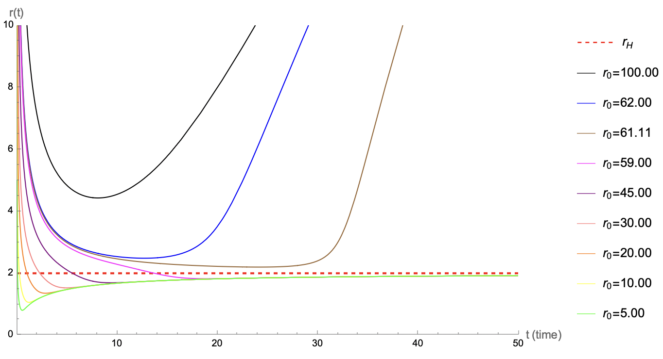
(b) $\omega\gg M$, for the parameters $\omega=10^{4}$ and $M=1$.

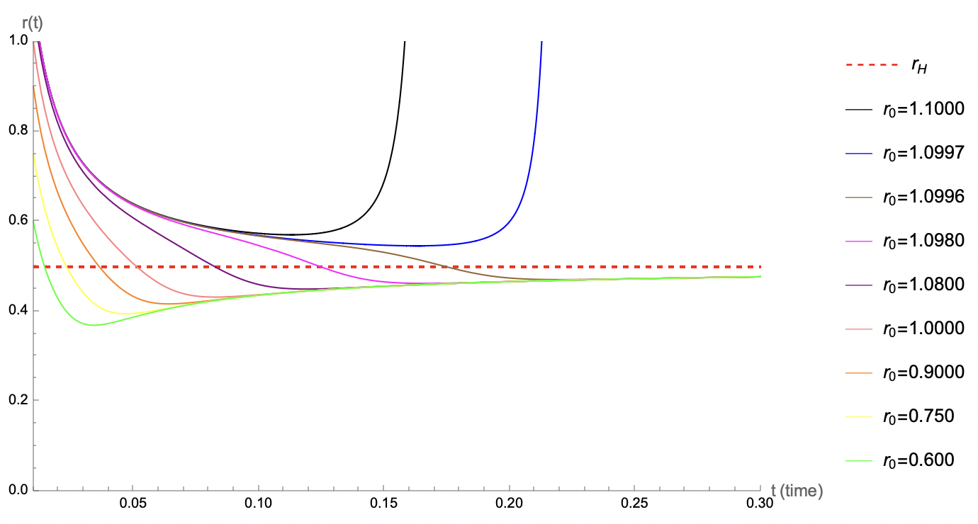
(c) $\omega\ll M$, for the parameters $\omega=1$ and $M=10^{2}$.

Figure 2: Geodesic representation of the Schwarzschild-like black hole (30), considering different limits. For the representation, the initial radius is denoted by $r_{0}$, with initial time $t_{0}=0.01$.

Table 1 represents the estimated values for the event horizon, $r_{H}$, and the initial distance to the black hole (considering the initial time $t_{0}=0.01$), $r_{0,\text{crit}}$, after which for initial distance $r_{0}>r_{0,\text{crit}}$ the geodesic is no longer attracted to the black hole and diverge to the infinity. For that, we consider three values for the mass, $10^{-2}$, $1$ and $10^{2}$, and six different values to the Weyl constant for each $M$. We now analyze the impact of each of the parameters.

M	$\bm{\omega}$	$\bm{r_{H}}$	$\bm{r_{0,\text{crit}}}$
$10^{-2}$	$10^{-3}$	$4.87805\times 10^{-4}$	$4.898605\times 10^{-4}$
	$10^{-2}$	$4.0\times 10^{-3}$	$4.44686\times 10^{-3}$
	$10^{-1}$	$1.42857\times 10^{-2}$	$2.96460\times 10^{-2}$
	$1$	$1.92308\times 10^{-2}$	$5.55967\times 10^{-2}$
	$10^{1}$	$1.99203\times 10^{-2}$	$6.07338\times 10^{-2}$
	$10^{2}$	$1.99920\times 10^{-2}$	$6.12471\times 10^{-2}$
$1$	$10^{-2}$	$4.98753\times 10^{-3}$	$2.05553\times 10^{-3}$
	$10^{-1}$	$4.87805\times 10^{-2}$	$6.97344\times 10^{-2}$
	$1$	$0.4$	$2.440224$
	$10^{1}$	$1.42857$	$2.87911\times 10^{1}$
	$10^{2}$	$1.92308$	$5.57693\times 10^{1}$
	$10^{3}$	$1.99203$	$6.05870\times 10^{1}$
$10^{2}$	$10^{-1}$	$4.99875\times 10^{-2}$	$5.21649\times 10^{-2}$
	$1$	$4.98753\times 10^{-1}$	$1.09968$
	$10^{1}$	$4.87805$	$5.714214\times 10^{1}$
	$10^{2}$	$4.0\times 10^{1}$	$2.43480\times 10^{3}$
	$10^{3}$	$1.42857\times 10^{2}$	$2.87908\times 10^{4}$
	$10^{4}$	$1.92308\times 10^{2}$	$5.57693\times 10^{4}$

Table 1: Estimated values for the event horizon, $r_{H}$, and the initial distance to the black hole, after which the geodesic is no longer attracted to the black hole and diverges to infinity, $r_{0,\text{crit}}$, considering different values to the mass and the Weyl parameters, $M$ and $\omega$, respectively.

In Figure 3, we show the numerical analysis of the relation between the mass of the black hole, $M$, the Weyl constant, $\omega$, and the results of the event horizon, $r_{H}$, and the critical radius, $r_{0,\text{crit}}$. For that, it was be considered 35 different values for the Weyl constant, for each of the masses, and $r_{H}$ and $r_{0,\text{crit}}$ were calculated numerically for each of the cases. Considering this analysis we can conclude that the global behavior of both quantities are similar regardless of the mass of the black holes (small or large) of the used values for the Weyl constant. We can also conclude that there is an asymptotic behavior in the loglog representation for the event horizon and for the critical initial value of the distance for which the geodesic is no longer attracted to the black hole, and the higher the event horizon is, the higher this distance is found.

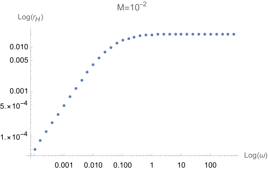
(a) Behavior of $r_{H}$ compared to $\omega$, considering the black hole mass $M=10^{-2}$.

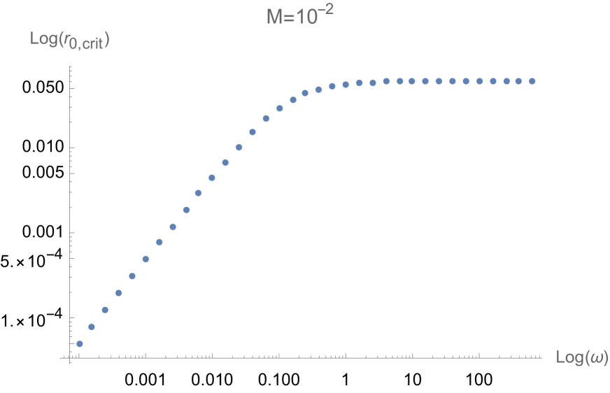
(b) Behavior of $r_{0,\text{crit}}$ compared to $\omega$, considering the black hole mass $M=10^{-2}$.

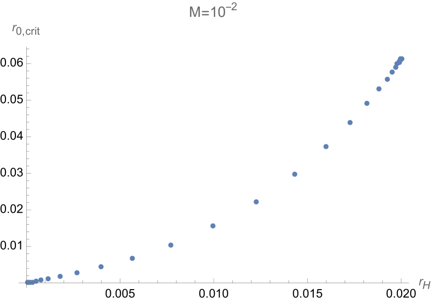
(c) Behavior of $r_{H}$ compared to $r_{0,\text{crit}}$, considering the black hole mass $M=10^{-2}$.

(d) Behavior of $r_{H}$ compared to $\omega$, considering the black hole mass $M=1$.

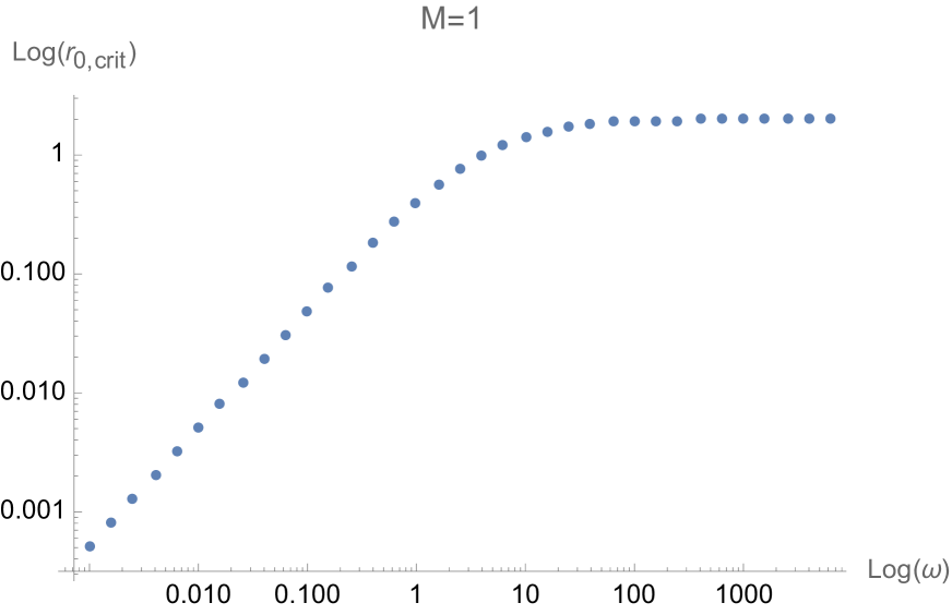
(e) behavior of $r_{0,\text{crit}}$ compared to $\omega$, considering the black hole mass $M=1$.

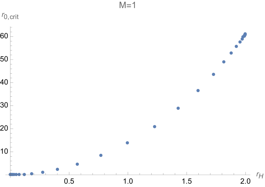
(f) Behavior of $r_{H}$ compared to $r_{0,\text{crit}}$, considering the black hole mass $M=1$.

(g) Behavior of $r_{H}$ compared to $\omega$, considering the black hole mass $M=10^{2}$.

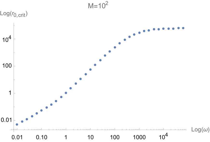
(h) Behavior of $r_{0,\text{crit}}$ compared to $\omega$, considering the black hole mass $M=10^{2}$.

(i) Behavior of $r_{H}$, compared to $r_{0,\text{crit}}$, considering the black hole mass $M=10^{2}$.

Figure 3: Analysis of the relation between the mass of the black hole, $M$, the Weyl constant, $\omega$, and the results of the event horizon, $r_{H}$, and the critical radius, $r_{0,\text{crit}}$, after that for initial distance $r_{0}>r_{0,\text{crit}}$ the geodesic is no longer attracted to the black hole and diverge to the infinity.

3.1.2 Second Case: $A_{\mu}=(A_{0}(r),A_{1}(r),0,0)$

We now consider the second possible ansatz for the Weyl vector field, namely $A_{\mu}=\left(A_{0}(r),A_{1}(r),0,0\right)$, with $A_{0}(r)\neq 0$ and $A_{1}(r)\neq 0$ arbitrary functions that obey the constraint equation:

$$A_{0}^{\prime}(r)+(A_{1}(r)-\alpha^{\prime}(r))A_{0}(r)=0.$$ (33)

Using this relation to $A_{1}(r)$ and comparing the time-time and the radial-radial components of the Eqs. (27a), we obtain the equation:

$$2rA_{0}^{\prime\prime}(r)-A_{0}^{\prime}(r)\left(r\left(\alpha^{\prime}(r)+\beta^{\prime}(r)\right)-4\right)=0.$$ (34)

Analogously to the previous case, we assume $\beta(r)=-\alpha(r)+\epsilon$, with $\epsilon$ some constant, together with the field equations (27), such that we find:

$$A_{0}(r) =\frac{1}{\omega}\left(1-\frac{2M}{r}\right),$$ (35a)

$$A_{1}(r) =\frac{2r}{r^{2}-4\omega^{2}}$$ (35b)

$$e^{\alpha(r)} =1-\frac{2M}{r}+\frac{M}{2\omega}\left(\frac{r}{\omega}\right)-\frac{1}{4}\left(\frac{r}{\omega}\right)^{2},$$ (35c)

$$e^{\beta(r)} =\frac{1}{1-\frac{2M}{r}+\frac{M}{2\omega}\left(\frac{r}{\omega}\right)-\frac{1}{4}\left(\frac{r}{\omega}\right)^{2}},\vspace{0.5cm}$$ (35d)

where $M>0$ is the black hole mass and $\omega$ is the Weyl constant. We note that the relation between the time-time and radial-radial components of the metric is $g_{11}=-\frac{1}{g_{00}}$, considering, without loss generality, $\epsilon=0$.

It is easy to see that, performing $g_{00}=0$, we can obtain two event horizons, which occurs when $r^{{}^{(M)}}_{H}=2M$ and $r^{{}^{(\omega)}}_{H}=2|\omega|$. This results resembles the black hole and cosmological horizons discussion Shankaranarayanan [2003].

In order to understand the possible values to $\omega$, we will apply the constraint (22b) considering three different cases: $\omega=M$; $|\omega|>M$; $|\omega|<M$. In the first case, considering $\omega=M$, we only have one event horizon, $R_{H}=2M$. The constraint (22b) is automatically satisfied, outside the event horizon, for any $M>0$. In the second case, $|w|>M$, we have two event horizons and the external one is the $r^{{}^{(\omega)}}_{H}$. The constraint (22b) is satisfied for any $r>r^{{}^{(\omega)}}_{H}$ if and only if $\omega>0$. Finally, when $|w|<M$, we also have two event horizons and the external one is the $r^{{}^{(M)}}_{H}$. The constraint (22b) is satisfied for any $r>r^{{}^{(M)}}_{H}$ also if and only if $\omega>0$. Therefore, in general, we have to impose that $\omega>0$.

Analyzing, globally, the Weyl vector, we can see that $A_{0}(r)\to\frac{1}{\omega}$ and $A_{1}(r)\to 0$, when $r\to\infty$. In fact, if we require spacetime to be asymptotically flat, then $\omega\gg 1$, but if we expect that at infinity we can have non-zero background, then we see that the vector field contributes cosmologically at infinity with $A_{0}=1/\omega$.

In this gravity model under study, a Schwarzschild-like black hole can exist with a non-zero Ricci scalar. Although the total curvature scalar is zero, the Ricci scalar takes the form

$$R=\frac{3(r-M)}{\omega^{2}r}.$$ (36)

We can get the global behavior for the Ricci scalar graphically in Fig. 4. It is possible to see that, in the limit $r\to\infty$, the Ricci scalar $R\to\frac{3}{\omega^{2}}$. We also can note that the Ricci curvature is zero when $r=M$, i.e. on the surface of the black hole. When $\omega>M$, the Ricci scalar in the external event horizon is given by $R\left(r^{{}^{(\omega)}}_{H}\right)=\frac{3(2\omega-M)}{2\omega^{3}}$. When $\omega\leq M$, the Ricci scalar in the external event horizon is given by $R\left(r^{{}^{(M)}}_{H}\right)=\frac{3}{2\omega^{2}}$.

Figure 4: Global behavior of the standard Ricci scalar (built from the Levi-Civita part of the connection) as function of the distance, assuming $\omega=1$ and $M=1$.

Using the relation, Eq. (15), we derive the geodesics equation. Firstly, we note that in this case $f^{\alpha}=0$, so the geodesics equation is the usual one from GR.

Let’s further consider $u^{\alpha}=(t(s),r(s),0,0)$. Therefore, the trajectory described by the geodesics can be given by

$$\frac{dr}{dt}=\frac{\Gamma_{00}^{1}t^{2}+\Gamma_{11}^{1}r^{2}}{2\Gamma_{01}^{0}tr}.$$ (37)

These three scenarios can be explored graphically. The numerical solutions of the geodesic equation, Eq. (37), are shown in Fig.5: Fig. 5(a) for $\omega=M$, Fig. 5(b) for $\omega\gg M$ and Fig. 5(c) for $\omega\ll M$.

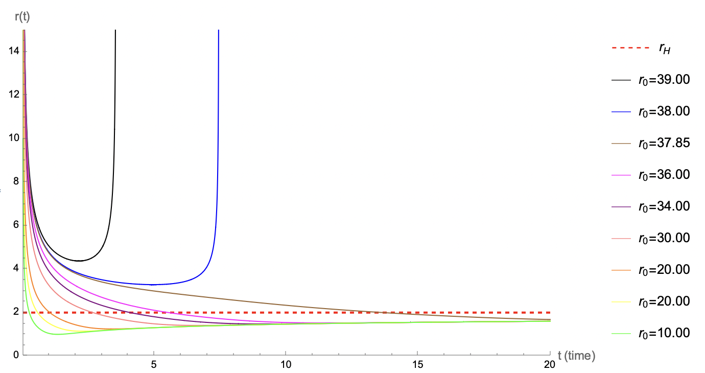
(a) $\omega=M$, for the parameters $\omega=1$ and $M=1$.

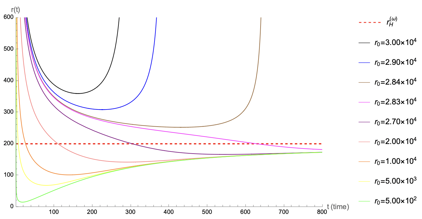
(b) $\omega\gg M$, for the parameters $M\omega=10^{2}$ and $M=1$.

(c) $\omega\ll M$, for the parameters $\omega=1$ and $M=10^{2}$.

Figure 5: Geodesic representation of the Schwarzschild-like black hole (35), considering different limits. For the representation, the initial radius is denoted by $r_{0}$, with initial time $t_{0}=0.01$.

We complement the analysis with a table, namely Table 2, which represents the estimated values for the external event horizon, $r_{H,\text{ext}}$ ($r_{H}^{{}^{(\omega)}}$ or $r_{H}^{{}^{(M)}}$), depending on the value of the parameters), and the initial distance to the black hole (considering the initial time $t_{0}=0.01$), $r_{0,\text{crit}}$, after that for initial distance $r_{0}>r_{0,\text{crit}}$ the geodesic is no longer attracted to the black hole and diverges to the infinity. For that, we consider three types of masses, $10^{-2}$, $1$ and $10^{2}$, and six different values to the Weyl constant for each $M$. Here, we intend to analyze the impact of each of the parameters.

M	$\bm{\omega}$	$\bm{r_{H,\text{ext}}}$	$\bm{r_{0,\text{crit}}}$
$10^{-2}$	$10^{-3}$	$2.0\times 10^{-2}$	$2.03962\times 10^{-2}$
	$10^{-2}$	$2.0\times 10^{-2}$	$4.74587\times 10^{-2}$
	$10^{-1}$	$2.0\times 10^{-1}$	$9.40337\times 10^{-1}$
	$1$	$2.0$	$2.84252\times 10^{1}$
	$10^{1}$	$2.0\times 10^{1}$	$8.94872\times 10^{2}$
	$10^{2}$	$2.0\times 10^{2}$	$2.82857\times 10^{4}$
$1$	$10^{-2}$	$2.0$	$2.03925$
	$10^{-1}$	$2.0$	$4.12739$
	$1$	$2.0$	$3.79018\times 10^{1}$
	$10^{1}$	$2.0\times 10^{1}$	$9.17359\times 10^{2}$
	$10^{2}$	$2.0\times 10^{2}$	$2.83548\times 10^{4}$
	$10^{3}$	$2.0\times 10^{3}$	$8.94650\times 10^{5}$
$10^{2}$	$10^{-1}$	$2.0\times 10^{2}$	$2.03924\times 10^{2}$
	$1$	$2.0\times 10^{2}$	$4.12172\times 10^{2}$
	$10^{1}$	$2.0\times 10^{2}$	$3.41783\times 10^{3}$
	$10^{2}$	$2.0\times 10^{2}$	$3.77465\times 10^{4}$
	$10^{3}$	$2.0\times 10^{3}$	$9.17119\times 10^{5}$
	$10^{4}$	$2.0\times 10^{4}$	$2.83541\times 10^{7}$

Table 2: Estimated values for the external event horizon, $r_{H,\text{ext}}$, and the initial distance to the black hole, after which the geodesic is no longer attracted to the black hole and diverges to infinity, $r_{0,\text{crit}}$, considering different values to the mass and the Weyl parameters, $M$ and $\omega$ respectively.

In Figure 6, it is represented the numerical analysis of the relation between the mass of the black hole, $M$, the Weyl constant, $\omega$, and the results of the external event horizon, $r_{H,\text{ext}}$, and the critical radius, $r_{0,\text{crit}}$. For that, it was be considered 35 different values for the Weyl constant, for each of the masses, and $r_{H,\text{ext}}$ and $r_{0,\text{crit}}$ were calculated numerically for each of the cases. Considering this analysis we can conclude that the global behavior of both quantities may follow the previous analysis. Due to numerical simulations limitations, we cannot plot much further (higher values for $\omega$), therefore we cannot directly compare with the general behavior from the first ansatz for the Weyl vector field. We note, however, that this case has two horizons (possibly a black hole and a cosmological ones, see e.g. Ref. Shankaranarayanan [2003], Mureika et al. [2016b]).

(a) Behavior of $r_{H,\text{ext}}$ compared to $\omega$, considering the black hole mass $M=10^{-2}$.

(b) Behavior of $r_{0,\text{crit}}$ compared to $\omega$, considering the black hole mass $M=10^{-2}$.

(c) Behavior of $r_{H,\text{ext}}$ compared to $r_{0,\text{crit}}$, considering the black hole mass $M=10^{-2}$.

(d) Behavior of $r_{H,\text{ext}}$ compared to $\omega$, considering the black hole mass $M=1$.

(e) Behavior of $r_{0,\text{crit}}$ compared to $\omega$, considering the black hole mass $M=1$.

(f) Behavior of $r_{H,\text{ext}}$ compared to $r_{0,\text{crit}}$, considering the black hole mass $M=1$.

(g) Behavior of $r_{H,\text{ext}}$ compared to $\omega$, considering the black hole mass $M=10^{2}$.

(h) Behavior of $r_{0,\text{crit}}$ compared to $\omega$, considering the black hole mass $M=10^{2}$.

(i) Behavior of $r_{H,\text{ext}}$, compared to $r_{0,\text{crit}}$, considering the black hole mass $M=10^{2}$.

Figure 6: Analysis of the relation between the mass of the black hole, $M$, the Weyl constant, $\omega$, and the results of the external event horizon, $r_{H,\text{ext}}$, and the critical radius, $r_{0,\text{crit}}$, after that for initial distance $r_{0}>r_{0,\text{crit}}$ the geodesic is no longer attracted to the black hole and diverge to the infinity.

3.2 Cosmological Constant Background

In this section, we will analyze the black hole solutions when the matter Lagrangian density is non-vanishing. For simplicity and in order to grasp the first non-trivial solutions we shall consider it in the form of a cosmological constant, i.e., a constant energy density. Considering $\mathcal{L}^{{}^{(\Lambda)}}=-2\Lambda$, the energy-momentum tensor components are given by

$$T^{{}^{(\Lambda)}}_{\mu\nu}=-2\Lambda g_{\mu\nu}.$$ (38)

The field equations (9) take the form

$$\bar{R}_{\mu\nu}\left(F_{1}(\bar{R})-2\Lambda F_{2}(\bar{R})\right)-\frac{1}{2}\left(f_{1}(\bar{R})-2\Lambda f_{2}(\bar{R})\right)=0.$$ (39)

Taking the trace of these equations, we obtain the relation

$$f_{1}(\bar{R})-2\Lambda f_{2}(\bar{R})=\gamma\bar{R}^{2}+\xi,$$ (40)

where $\gamma$ and $\xi$ are constants.

So, the field equations are

$$\bar{R}_{\mu\nu}-\frac{1}{4}g_{\mu\nu}\bar{R}=0,$$ (41)

that implies that

$$\bar{R}_{\mu\nu}=0,$$ (42)

$$\bar{R}=0.$$ (43)

It is straightforward to verify that, taking Eq. (43) and Eq.(40) into account, both constraint equation (8) and the non-conservation law (12) are automatically satisfied, for any vector field $A_{\lambda}$. So the vacuum solutions found above are also solutions when we consider a Cosmological Constant Background. Therefore, we can interpret this result as stemming from the mathematical reparametrization, namely $f(\bar{R})=f_{1}(\bar{R})-2\Lambda f_{2}(\bar{R})$ in Eq. (40). However, as discussed in Ref. Bertolami et al. [2015], physically these two models are distinct as one has a physical meaning for the cosmological constant-like Lagrangian (the energy from vacuum). Thus, we can relate this ”cosmological constant” with a cosmological constant appearing as an integration constant of the field equations. The non-minimal coupling model has an advantage of allowing for contributing for an explanation of the so-called cosmological constant problem.

3.3 Thermodynamics

We now evaluate some thermodynamics quantities for the black hole solutions found in this paper for the non-minimally coupled Weyl connection gravity model. We follow closely Refs. Gomes et al. [2020], Sebastiani and Zerbini [2011], Mureika et al. [2016b] in order to compute such quantities.

Therefore, for the metric (20), the black hole temperature from the quantum tunneling method (which is equivalent to the Hawking method Gomes et al. [2020], and we denote by the superscript ”BH”) is given by

$$T^{{(BH)}}=\frac{\sqrt{e^{\alpha(r_{H,\text{ext}})^{\prime}}e^{-\beta(r_{H,\text{ext}})^{\prime}}}}{4\pi}=\frac{\sqrt{-\alpha^{\prime}(r_{H,\text{ext}})\beta^{\prime}(r_{H,\text{ext}})e^{\alpha(r_{H,\text{ext}})-\beta(r_{H,\text{ext}})}}}{4\pi}.$$ (44)

The black hole entropy is given by

$$S^{{(BH)}}=\int\frac{dM}{T^{{(BH)}}(M)}$$ (45)

and the black hole heat capacity at constant volume takes the form

$$C_{V}^{{(BH)}}=T^{{(BH)}}\frac{\partial S^{{(BH)}}}{\partial T^{{(BH)}}}=T^{{(BH)}}\frac{\partial S^{{(BH)}}}{\partial r_{H,\text{ext}}}\left(\frac{\partial T^{{(BH)}}}{\partial r_{H,\text{ext}}}\right)^{-1}.$$ (46)

We can also derive such quantities from the so-called ”area approach”. Thus, the area temperature reads:

$$T^{{}^{(A)}}=\frac{r_{H,\text{ext}}-r_{H,\text{int}}}{4\pi r_{H,\text{ext}}^{2}}.$$ (47)

Analogously, the area entropy is:

$$S^{{}^{(A)}}=\frac{A(r_{H,\text{ext}})}{4},$$ (48)

and the area specific heat capacity:

$$C_{V}^{{}^{(A)}}=T^{{}^{(A)}}\frac{\partial S^{{}^{(A)}}}{\partial T^{{}^{(A)}}}=T^{{}^{(A)}}\frac{\partial S^{{}^{(A)}}}{\partial r_{H,\text{ext}}}\left(\frac{\partial T^{{}^{(A)}}}{\partial r_{H,\text{ext}}}\right)^{-1}.$$ (49)

When both definitions do not coincide, then we need to modify the first law of thermodynamics Ma and Zhao [2014], Maluf and Neves [2018], Gomes et al. [2020], likewise the non-minimal coupling model has bearings on the second law Bertolami and Gomes [2020], such that:

$$dM=TdS\implies T^{{}^{(A)}}dS^{{}^{(A)}}=T^{{}^{(BH)}}dS^{{}^{(BH)}}\leavevmode\nobreak\ ,$$ (50)

from which one can parametrize:

$$T^{{}^{(BH)}}dS^{{}^{(BH)}}=L^{{}^{(A)}}dM\leavevmode\nobreak\ ,$$ (51)

where $L^{{}^{(A)}}=T^{{}^{(A)}}\frac{dS^{{}^{(A)}}}{dM}$ is a function to be determined Gomes et al. [2020].

Finally, for both definitions, the free energy stems from:

$$F=M-TS\leavevmode\nobreak\ .$$ (52)

We now apply these definitions to each solution found for the Schwarzschild-like black holes.

3.3.1 Schwarzschild-like Black Bole: First Case

Considering the solution (30), the previous thermodynamical quantities read:

$$T^{{(BH)}} =T_{0}\left(1+6\frac{M}{\omega}\right)^{-3/2},$$ (53a)

$$S^{{(BH)}} =\frac{8\pi}{9}\left(1+6\frac{M}{\omega}\right)^{-3/2}(3M+\omega)(6M+\omega),$$ (53b)

$$C_{V}^{{(BH)}} =C_{0}\left(1+6\frac{M}{\omega}\right)^{-3/2}\frac{6M+\omega}{\omega-3M},$$ (53c)

where $T_{0}=\frac{1}{8\pi M}$ and $C_{0}=-8\pi M^{2}$ are the Hawking temperature and the heat capacity at constant volume for the usual Schwarzschild black hole, respectively. This expression for the specific heat means that black hole is stable for $\omega>3M$, and unstable for $\omega<3M$ as the black hole will evaporate leaving a stable cold remnant, in contrast with standard Schwarzschild black holes in GR which are always unstable as its temperature increases as it absorbs mass. The specific heat diverges at $\omega=3M$ despite not corresponding to the maximum temperature which is a decreasing function of the mass and has a maximum at zero mass, i.e., $T_{\text{max}}=T_{0}$. Nonetheless, this might signal the existence of a thermodynamical critical transition point.

Using the relation (52), the free-energy considering the tunneling method takes the form

$$F^{{}^{(BH)}}=-\left(M+\omega+\frac{\omega^{2}}{9M}\right)\leavevmode\nobreak\ ,$$ (54)

which can be minimized when $\omega=0$ and $M\neq 0$. Thus, the system in the quantum tunneling description can be globally stable, as it allows for non-vanishing masses to minimise its free energy.

We now proceed to compute the previous quantities in the area method. We draw our attention to the fact that there is only one event horizon, namely $r_{H}=2M\frac{\omega}{4M+\omega}$, thus being formally equivalent to impose $r_{H,int}=0$.

Therefore, the area temperature is:

$$T^{{}^{(A)}}=T_{0}\frac{4M+\omega}{\omega},$$ (55)

whilst the area entropy reads:

$$S^{{}^{(A)}}=4\pi\left(\frac{M\omega}{4M+\omega}\right)^{2},$$ (56)

and the area specific heat capacity at constant volume is written as:

$$C_{V}^{{}^{(A)}}=C_{0}\left(\frac{\omega}{4M+\omega}\right)^{2}\leavevmode\nobreak\ ,$$ (57)

which is always positive definite, thus the system is locally stable for all values of the mass and of the Weyl constant.

Using the relation (52), the free-energy considering the ”area approach” takes the form

$$F^{{}^{(A)}}=\frac{M\left(8M+\omega\right)}{2\left(4M+\omega\right)}\leavevmode\nobreak\ ,$$ (58)

which is minimized for $M=0$, thus the system is globally unstable in the area method.

Since the area and quantum tunneling methods lead to different results, then the first law must be revisited Gomes et al. [2020]. In this case, the function $L^{{}^{(A)}}=\frac{\omega^{2}}{(4M+\omega)^{2}}$.

3.3.2 Schwarzschild-like Black Bole: Becond Case

Considering the solution (35) and applying the expression (44), considering the external event horizon, it is possible to see that $T^{{}^{(BH)}}$ is purely imaginary and diverges, which is non-physical:

$$T^{{}^{(BH}}=\frac{i}{2\pi r}\left|\frac{r^{3}-M(r^{2}+4\omega^{2})}{(r-2M)(r^{2}-4\omega^{2})}\right|.$$ (59)

If we instead compute the thermodynamical quantities via the ”area approach”, we have three cases to be analyzed.

The first case corresponds to $\omega<M$, for which the two event horizons read $r_{H,\text{int}}=2\omega$ and $r_{H,\text{ext}}=2M$. Thus, the area temperature is

$$T^{{}^{(A)}}=T_{0}\left(1-\frac{\omega}{M}\right)\leavevmode\nobreak\ ,$$ (60)

which is always positive and does not diverge.

As for the area entropy:

$$S^{{}^{(A)}}=4\pi M^{2}\leavevmode\nobreak\ ,$$ (61)

and the specific heat at constant volume:

$$C_{V}^{{}^{(A)}}=C_{0}\frac{\omega-M}{2\omega-M}\leavevmode\nobreak\ ,$$ (62)

which is positive when $\omega<M<2\omega$, negative when $2\omega<M$ and diverges at $M=2\omega$. This critical point does not correspond to the maximum value of the temperature that occurs for a vanishing Weyl constant and has the value of $T_{\text{max}}=T_{0}$. Nevertheless, one can see that the system is locally unstable for negative values of the specific heat, and stable for positive ones.

The free energy is given by:

$$F^{{}^{(A)}}=\frac{\omega+M}{2}\leavevmode\nobreak\ ,$$ (63)

which is minimized for both vanishing mass and Weyl constant.

As for the second case, namely when $\omega>M$, we have $r_{H,\text{int}}=2M$ and $r_{H,\text{ext}}=2\omega$. Thus, the area temperature is:

$$T^{{}^{(A)}}=T_{0}\frac{M}{\omega}\left(1-\frac{M}{\omega}\right)\leavevmode\nobreak\ ,$$ (64)

which is always positive and does not diverge.

The area entropy now reads:

$$S^{{}^{(A)}}=4\pi\omega^{2}\leavevmode\nobreak\ ,$$ (65)

and the specific heat:

$$C_{V}^{{}^{(A)}}=C_{0}\left(\frac{\omega}{M}\right)^{2}\frac{M-\omega}{2M-\omega}\leavevmode\nobreak\ ,$$ (66)

which is positive when $M<\omega<2M$ and this Shwarzschild-like black hole evaporates to a locally stable cold remnant, negative when $2M<\omega$ and diverges for $\omega=2M$. In this case, the critical point of the specific heat corresponds to the maximum of the temperature, $T_{\text{max}}=\frac{T_{0}}{4}$.

The free energy is given by:

$$F^{{}^{(A)}}=\frac{3M-\omega}{2}\leavevmode\nobreak\ ,$$ (67)

which can be positive, null, or negative.

The third case corresponds to $\omega=M$, for which $r_{H}=2M$. Therefore, the area temperature reads:

$$T^{{}^{(A)}}=T_{0}\leavevmode\nobreak\ ,$$ (68)

the area entropy is:

$$S^{{}^{(A)}}=4\pi M^{2}\leavevmode\nobreak\ ,$$ (69)

and the specific heat at constant volume is

$$C_{V}^{{}^{(A)}}=C_{0}\leavevmode\nobreak\ .$$ (70)

Finally, the free energy is:

$$F^{{(A)}}=\frac{M}{2}\leavevmode\nobreak\ ,$$ (71)

which is minimized only for $M=0$, thus being the system globally unstable.

This case reproduces the behavior of GR’s non-rotating black holes.

Since the area and quantum tunneling methods lead to different results in this second case as well, then the first law must be revisited Gomes et al. [2020]. However, in this case, it is not possible to fully determine the function $L^{{}^{(A)}}$ since the quantum tunneling leads to divergent quantities.

4 Reissner-Nordstrøm-like Black Hole

In this section, we will analyze black hole solutions of the form of Reissner-Nordstrøm, i.e., black holes which are static, have mass and electric charge. In order to describe the gravitational field outside a charged, non-rotating, spherically symmetric body, we consider the electrostatic four-potential $\Phi_{\mu}=(-\phi(r),0,0,0)$, with $\phi(r)$ the scalar potential. Using the relation (18), it is possible to see that $\mathcal{L}^{{}^{(EM)}}=\frac{1}{2}e^{-\alpha(r)-\nu(r)}\phi^{\prime}(r)^{2}$ and the energy momentum-tensor is such that

$$T^{{(EM)}\mu}_{\nu}=\text{diag}(-1,-1,1,1)\frac{1}{2}e^{-\alpha(r)-\beta(r)}\phi^{\prime}(r)^{2}.$$ (72)

Applying the previous result into Maxwell equations (19), it follows that

$$\phi^{\prime}(r)=-e^{\frac{1}{2}(\alpha(r)+\beta(r))}\frac{c_{1}}{f_{2}(\bar{R})r^{2}},$$ (73)

with $c_{1}$ being some constant, which we identify with the electric charge, $Q$, in analogy with the GR’s result.

Analogously to the Schwarzchild-like solutions, we shall look into vacuum and the first simplest contribution from non-vacuum Lagrangian density.

4.1 Vacuum Background

We now consider a vacuum background. Thus, the contribution to the energy-momentum tensor is given only by the black hole geometry seen from the infinity as a point charge.

First of all, it should be noted that $\Theta(\bar{R})\neq 0$. Otherwise, equations (11) imply zero energy-momentum tensor, since $T^{{}^{(EM)}}=0$. Therefore, the only applicable Weyl vector is the radial one, Eq. (21a).

From the trace of the field equations (10), we have

$$f_{1}(\bar{R})=\frac{1}{2}\bar{R}\Theta(\bar{R}).$$ (74)

Applying this result, together with the fact that $F_{1}(\bar{R})=\frac{df_{1}(\bar{R})}{d\bar{R}}$ and the constraint (8), we obtain

$$F_{1}(\bar{R})=\frac{1}{2}\left(1-A(r)\frac{\bar{R}}{\bar{R}^{\prime}}\right)\Theta(\bar{R}),$$ (75)

when $\bar{R}^{\prime}\neq 0$.

Using this relation, together with $\Theta(\bar{R})=F_{1}(\bar{R})+\mathcal{L}F_{2}(\bar{R})$ and the non-conservation equation to energy-momentum tensor (12), it is possible to observe that $f_{2}(R)=0$. So, we conclude that it is not possible to derive a charged black hole solution, in vacuum, for any static and spherical metric in the model under study.

If $\bar{R}^{\prime}=0$, it is also impossible to obtain a black hole solution. In fact, $\bar{R}^{\prime}=0$ implies that the curvature scalar is constant, so $\Theta(\bar{R})$ is also constant. From the constraint (8), this imply that $A(r)=0$.

4.2 Cosmological Constant Background

We now consider a charged black hole immersed in a cosmological constant background. Then, the Lagrangian density is given by $\mathcal{L}=\mathcal{L}^{{}^{(EM)}}+\mathcal{L}^{{}^{(\Lambda)}}$ and the components of the energy momentum tensor are $T_{\mu\nu}=T^{{}^{(EM)}}_{\mu\nu}+T^{{}^{(\Lambda)}}_{\mu\nu}$ as described above.

It should be noted that, again, $\Theta(\bar{R})\neq 0$. Otherwise, equations (11) imply zero energy-momentum tensor, since $T^{{}^{(EM)}}=0$. Therefore, the only viable ansatz for the Weyl vector is the radial one, Eq. (21a).

By combining all trace-free equations (11), it is possible to find a similar equation to (28). Therefore, we will use the same relation $\beta(r)=-\alpha(r)+\epsilon$. With this assumption, it is possible to see that the solution to $A(r)$ is, again,

$$A(r)=\frac{2}{r+\omega},$$ (76)

with $\omega>0$.

So, from (8), we obtain

$$\Theta(\bar{R})=\frac{\xi}{(r+\omega)^{2}},$$ (77)

with $\xi$ some integration constant that we will define later.

Using this result in all previous equations, it is possible to obtain that the appropriated model is given by

$$f_{1}(\bar{R}) =\gamma\bar{R}^{2}+2\Lambda\zeta$$ (78a)

$$f_{2}(\bar{R}) =\zeta,$$ (78b)

where $\gamma=\xi\frac{(6\tilde{Q}^{2}+6M\omega+\omega^{2})}{72\tilde{Q}^{2}}$, $\xi=\frac{\omega^{2}}{4}\zeta$, $\zeta$ some constant and $\tilde{Q}$ is the dressed charge such that the equation (73) gives

$$\phi(r)=\frac{\tilde{Q}}{r},$$ (79)

and we have the relation

$$Q^{2}=\zeta^{2}\tilde{Q}^{2}\left(1+6\left(\frac{M}{\omega}+\frac{\tilde{Q}^{2}}{\omega^{2}}\right)\right)^{-1},$$ (80)

where $Q$ is the usual charge.

The metric solution to this problem is given by

$$e^{\alpha(r)} =1-\frac{2M}{r}+\frac{\tilde{Q}^{2}}{r^{2}}+\frac{2\left(\omega^{2}+3M\omega+2\tilde{Q}^{2}\right)}{\omega^{2}}\frac{r}{\omega}+\frac{4M+\omega}{\omega}\left(\frac{r}{\omega}\right)^{2},$$ (81a)

$$e^{\beta(r)} =\frac{1+6\left(\frac{M}{\omega}+\frac{\tilde{Q}^{2}}{\omega^{2}}\right)}{1-\frac{2M}{r}+\frac{\tilde{Q}^{2}}{r^{2}}+\frac{2\left(\omega^{2}+3M\omega+2\tilde{Q}^{2}\right)}{\omega^{2}}\frac{r}{\omega}+\frac{4M+\omega}{\omega}\left(\frac{r}{\omega}\right)^{2}}.$$ (81b)

The curvature scalar takes the form

$$\bar{R}=\frac{36\tilde{Q}^{2}}{\left(\omega^{2}+6M\omega+6\tilde{Q}^{2}\right)\left(r+\omega\right)^{2}}.$$ (82)

It is easy to see that considering the limit $\tilde{Q}\rightarrow 0$, the curvature scalar $\bar{R}\rightarrow 0$ and the solution (81) converge to Schwarzschild-like solution (30).

Analyzing, globally, the curvature scalar (82) is positive for all $r$ and it decreases with distance from the black hole. The maximum value occurs when $r_{\text{max}}=0$, taking the value $\bar{R}_{\text{max}}=\frac{36\tilde{Q}^{2}}{\omega^{2}(\omega^{2}+6M\omega+6\tilde{Q}^{2})}$. In Figure 7, it is represented the global behavior of the scalar curvature as function of the distance, considering a specific case, where the point at which the external event horizon occurs is represented.

Figure 7: Global behavior of the scalar curvature $\bar{R}$ as function of the distance, assuming $M=10$, $\omega=1$ and $\tilde{Q}=1$.

The Ricci scalar takes the form

$$R=-\frac{12\left((4M+\omega)r^{2}+(\omega^{2}+3M\omega+2\tilde{Q}^{2})r-(\tilde{Q}^{2}+M\omega)\omega\right)}{r^{2}\omega\left(\omega^{2}+6M\omega+2\tilde{Q}^{2}\right)}$$ (83)

It is easy to see that considering the limit $\tilde{Q}\rightarrow 0$, the Ricci scalar $R$ converges to Schwarzschild-like solution (31). In Figure 8, it is represented the global behavior of the scalar curvature as function of the distance, considering a specific case, where the point at which the external event horizon occurs is represented.

Analyzing, globally, the Ricci scalar (83), it is possible to see that when $r\to 0$, the Ricci scalar goes to infinity, $R\to+\infty$. When $r\to\infty$, the Ricci scalar converge to a non-null constant, $R\to-\frac{12(\omega+4M)}{\omega(\omega^{2}+6M\omega+6\tilde{Q}^{2})}$. We can also note that the minimum value of Ricci scalar occurs when $r_{\text{min}}=\frac{2\omega\left(\tilde{Q}^{2}+M\omega\right)}{\omega^{2}+3M\omega+2\tilde{Q}^{2}}$ and takes the value $R_{\text{min}}=-\frac{3\left(4\tilde{Q}^{2}(\tilde{Q}^{2}+7M\omega+2\omega^{2})+\omega^{2}(5M+\omega)^{2}\right)}{\omega^{2}(\tilde{Q}^{2}+M\omega)(\omega^{2}+6M\omega+6\tilde{Q}^{2})}$.

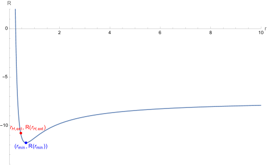
Figure 8: Global behavior of the standard Ricci scalar (built from the Levi-Civita part of the connection) as function of the distance, assuming $M=10$, $\omega=1$ and $\tilde{Q}=1$.

Due to the complexity of the solution obtained, it is not possible to provide a generic and complete analysis. We know that, under certain circumstances, we are in the presence of one or two event horizons, but it is difficult to rigorously define these values.

The Tables 3, 4 and 5 represent the estimated values for the internal, $r_{H,\text{int}}$, and external event horizon, $r_{H,\text{ext}}$, considering the mass values $10^{-2},\text{ }1\text{ and }10^{2}$, respectively. We can conclude that, for the cases where there is an event horizon which correspond to lower values for the effective charge provided the Weyl constant is above a certain lower limit, the values of both horizons are strikingly similar.

$\bm{\tilde{Q}}$	$\bm{\omega}$	$\bm{r_{H,\text{int}}}$	$\bm{r_{H,\text{ext}}}$
$10^{-4}$	$10^{-7}$	no $r_{H,\text{int}}$	no $r_{H,\text{ext}}$
	$10^{-6}$	no $r_{H,\text{int}}$	no $r_{H,\text{ext}}$
	$10^{-5}$	$5.0425\times 10^{-7}$	$4.6474\times 10^{-6}$
	$10^{-4}$	$5.0005\times 10^{-7}$	$4.9541\times 10^{-5}$
	$10^{-3}$	$5.0001\times 10^{-7}$	$4.8747\times 10^{-4}$
	$10^{-2}$	$5.0001\times 10^{-7}$	$3.9997\times 10^{-3}$
	$10^{-1}$	$5.0001\times 10^{-7}$	$1.4285\times 10^{-2}$
	$10^{1}$	$5.0001\times 10^{-7}$	$1.9920\times 10^{-2}$
	$10^{2}$	$5.0001\times 10^{-7}$	$1.9992\times 10^{-2}$
$10^{-3}$	$10^{-5}$	no $r_{H,\text{int}}$	no $r_{H,\text{ext}}$
	$10^{-4}$	no $r_{H,\text{int}}$	no $r_{H,\text{ext}}$
	$10^{-3}$	$5.0568\times 10^{-5}$	$4.5281\times 10^{-4}$
	$10^{-2}$	$5.0131\times 10^{-5}$	$3.9677\times 10^{-3}$
	$10^{-1}$	$5.0126\times 10^{-5}$	$1.4247\times 10^{-2}$
	$10^{0}$	$5.0126\times 10^{-5}$	$1.9183\times 10^{-2}$
	$10^{1}$	$5.0126\times 10^{-5}$	$1.9870\times 10^{-2}$
	$10^{3}$	$5.0126\times 10^{-5}$	$1.9949\times 10^{-2}$
	$10^{5}$	$5.0126\times 10^{-5}$	$1.9950\times 10^{-2}$
$10^{-}2$	for all $w>0$	no $r_{H,\text{int}}$	no $r_{H,\text{ext}}$
$10^{-}1$	for all $w>0$	no $r_{H,\text{int}}$	no $r_{H,\text{ext}}$
$1$	for all $w>0$	no $r_{H,\text{int}}$	no $r_{H,\text{ext}}$
$10^{1}$	for all $w>0$	no $r_{H,\text{int}}$	no $r_{H,\text{ext}}$
$10^{2}$	for all $w>0$	no $r_{H,\text{int}}$	no $r_{H,\text{ext}}$
$10^{3}$	for all $w>0$	no $r_{H,\text{int}}$	no $r_{H,\text{ext}}$
$10^{4}$	for all $w>0$	no $r_{H,\text{int}}$	no $r_{H,\text{ext}}$

Table 3: Estimated values for the internal, $r_{H,\text{int}}$, and external event horizon, $r_{H,\text{ext}}$, considering the mass value $M=10^{-2}$ and different values to the charge and the Weyl parameters, $\tilde{Q}$ and $\omega$ respectively.

$\bm{\tilde{Q}}$	$\bm{\omega}$	$\bm{r_{H,\text{int}}}$	$\bm{r_{H,\text{ext}}}$
$10^{-4}$	$10^{-9}$	no $r_{H,\text{int}}$	no $r_{H,\text{ext}}$
	$10^{-8}$	no $r_{H,\text{int}}$	no $r_{H,\text{ext}}$
	$10^{-7}$	$5.0423\times 10^{-9}$	$4.6487\times 10^{-8}$
	$10^{-6}$	$5.0004\times 10^{-9}$	$4.9665\times 10^{-7}$
	$10^{-5}$	$5.0000\times 10^{-9}$	$4.9967\times 10^{-6}$
	$10^{-4}$	$5.0000\times 10^{-9}$	$4.9995\times 10^{-5}$
	$10^{-3}$	$5.0000\times 10^{-9}$	$4.9987\times 10^{-4}$
	$10^{-2}$	$5.0000\times 10^{-9}$	$4.9875\times 10^{-3}$
	$10^{-1}$	$5.0000\times 10^{-9}$	$4.8780\times 10^{-2}$
	$1$	$5.0000\times 10^{-9}$	$4.0000\times 10^{-1}$
	$10^{1}$	$5.0000\times 10^{-9}$	$1.4286\times 10^{0}$
	$10^{2}$	$5.0000\times 10^{-9}$	$1.9231\times 10^{0}$
	$10^{4}$	$5.0000\times 10^{-9}$	$1.9992\times 10^{0}$
$10^{-3}$	$10^{-7}$	no $r_{H,\text{int}}$	no $r_{H,\text{ext}}$
	$10^{-6}$	no $r_{H,\text{int}}$	no $r_{H,\text{ext}}$
	$10^{-5}$	$5.0423\times 10^{-7}$	$4.6487\times 10^{-6}$
	$10^{-4}$	$5.0004\times 10^{-7}$	$4.9664\times 10^{-5}$
	$10^{-3}$	$5.0000\times 10^{-7}$	$4.9954\times 10^{-4}$
	$10^{-2}$	$5.0000\times 10^{-7}$	$4.9872\times 10^{-3}$
	$10^{-1}$	$5.0000\times 10^{-7}$	$4.8780\times 10^{-2}$
	$1$	$5.0000\times 10^{-7}$	$4.0000\times 10^{-1}$
	$10^{1}$	$5.0000\times 10^{-7}$	$1.4286\times 10^{0}$
$10^{-2}$	$10^{-5}$	no $r_{H,\text{int}}$	no $r_{H,\text{ext}}$
	$10^{-4}$	no $r_{H,\text{int}}$	no $r_{H,\text{ext}}$
	$10^{-3}$	$5.0425\times 10^{-5}$	$4.6474\times 10^{-4}$
	$10^{-2}$	$5.0005\times 10^{-5}$	$4.9541\times 10^{-3}$
	$10^{-1}$	$5.0001\times 10^{-5}$	$4.8747\times 10^{-2}$
	$1$	$5.0001\times 10^{-5}$	$3.9997\times 10^{-1}$
	$10^{1}$	$5.0001\times 10^{-5}$	$1.4285\times 10^{0}$
	$10^{2}$	$5.0001\times 10^{-5}$	$1.9230\times 10^{0}$
	$10^{3}$	$5.0001\times 10^{-5}$	$1.9920\times 10^{0}$
$10^{-1}$	$10^{-3}$	no $r_{H,\text{int}}$	no $r_{H,\text{ext}}$
	$10^{-2}$	no $r_{H,\text{int}}$	no $r_{H,\text{ext}}$
	$10^{-1}$	$5.0568\times 10^{-3}$	$4.5281\times 10^{-2}$
	$1$	$5.0131\times 10^{-3}$	$3.9677\times 10^{-1}$
	$10^{1}$	$5.0126\times 10^{-3}$	$1.4247\times 10^{0}$
	$10^{2}$	$5.0126\times 10^{-3}$	$1.9183\times 10^{0}$
	$10^{3}$	$5.0126\times 10^{-3}$	$1.9870\times 10^{0}$
	$10^{4}$	$5.0126\times 10^{-3}$	$1.9942\times 10^{0}$
	$10^{5}$	$5.0126\times 10^{-3}$	$1.9949\times 10^{0}$
$1$	for all $w>0$	no $r_{H,\text{int}}$	no $r_{H,\text{ext}}$
$10^{1}$	for all $w>0$	no $r_{H,\text{int}}$	no $r_{H,\text{ext}}$
$10^{2}$	for all $w>0$	no $r_{H,\text{int}}$	no $r_{H,\text{ext}}$
$10^{3}$	for all $w>0$	no $r_{H,\text{int}}$	no $r_{H,\text{ext}}$
$10^{4}$	for all $w>0$	no $r_{H,\text{int}}$	no $r_{H,\text{ext}}$

Table 4: Estimated values for the internal,$r_{H,\text{int}}$, and external event horizon, $r_{H,\text{ext}}$, considering the mass value $M=1$ and different values to the charge and the Weyl parameters, $\tilde{Q}$ and $\omega$ respectively.

$\bm{\tilde{Q}}$	$\bm{\omega}$	$\bm{r_{H,\text{int}}}$	$\bm{r_{H,\text{ext}}}$
$10^{-4}$	$10^{-11}$	no $r_{H,\text{int}}$	no $r_{H,\text{ext}}$
	$10^{-10}$	no $r_{H,\text{int}}$	no $r_{H,\text{ext}}$
	$10^{-9}$	$5.0423\times 10^{-11}$	$4.6487\times 10^{-10}$
	$10^{-8}$	$5.0004\times 10^{-11}$	$4.9665\times 10^{-9}$
	$10^{-7}$	$5.0000\times 10^{-11}$	$4.9967\times 10^{-8}$
	$10^{-6}$	$5.0000\times 10^{-11}$	$4.9997\times 10^{-7}$
	$10^{-4}$	$5.0000\times 10^{-11}$	$5.0000\times 10^{-5}$
	$10^{-2}$	$5.0000\times 10^{-11}$	$4.9999\times 10^{-3}$
	$1$	$5.0000\times 10^{-11}$	$4.9875\times 10^{-1}$
	$10^{1}$	$5.0000\times 10^{-11}$	$4.8780\times 10^{0}$
	$10^{2}$	$5.0000\times 10^{-11}$	$4.0000\times 10^{1}$
	$10^{3}$	$5.0000\times 10^{-11}$	$1.4286\times 10^{2}$
	$10^{4}$	$5.0000\times 10^{-11}$	$1.9231\times 10^{2}$
	$10^{6}$	$5.0000\times 10^{-11}$	$1.9992\times 10^{2}$
$10^{-3}$	$10^{-9}$	no $r_{H,\text{int}}$	no $r_{H,\text{ext}}$
	$10^{-8}$	no $r_{H,\text{int}}$	no $r_{H,\text{ext}}$
	$10^{-7}$	$5.0423\times 10^{-9}$	$4.6487\times 10^{-8}$
	$10^{-6}$	$5.0004\times 10^{-9}$	$4.9665\times 10^{-7}$
	$10^{-5}$	$5.0000\times 10^{-9}$	$4.9967\times 10^{-6}$
	$10^{-4}$	$5.0000\times 10^{-9}$	$4.9997\times 10^{-5}$
	$10^{-3}$	$5.0000\times 10^{-9}$	$5.0000\times 10^{-4}$
	$10^{-2}$	$5.0000\times 10^{-9}$	$4.9999\times 10^{-3}$
	$10^{-1}$	$5.0000\times 10^{-9}$	$4.9987\times 10^{-2}$
	$1$	$5.0000\times 10^{-9}$	$4.9875\times 10^{-1}$
	$10^{1}$	$5.0000\times 10^{-9}$	$4.8780\times 10^{0}$
	$10^{2}$	$5.0000\times 10^{-9}$	$4.0000\times 10^{1}$
	$10^{3}$	$5.0000\times 10^{-9}$	$1.4286\times 10^{2}$
	$10^{5}$	$5.0000\times 10^{-9}$	$1.9920\times 10^{2}$
$10^{-2}$	$10^{-7}$	no $r_{H,\text{int}}$	no $r_{H,\text{ext}}$
	$10^{-6}$	no $r_{H,\text{int}}$	no $r_{H,\text{ext}}$
	$10^{-5}$	$5.0423\times 10^{-7}$	$4.6487\times 10^{-6}$
	$10^{-4}$	$5.0004\times 10^{-7}$	$4.9665\times 10^{-5}$
	$10^{-3}$	$5.0000\times 10^{-7}$	$4.9967\times 10^{-4}$
	$10^{-2}$	$5.0000\times 10^{-7}$	$4.9995\times 10^{-3}$
	$10^{-1}$	$5.0000\times 10^{-7}$	$4.9987\times 10^{-2}$
	$1$	$5.0000\times 10^{-7}$	$4.9875\times 10^{-1}$
	$10^{1}$	$5.0000\times 10^{-7}$	$4.8780\times 10^{0}$
	$10^{2}$	$5.0000\times 10^{-7}$	$4.0000\times 10^{1}$
	$10^{3}$	$5.0000\times 10^{-7}$	$1.4286\times 10^{2}$
	$10^{6}$	$5.0000\times 10^{-7}$	$1.9992\times 10^{2}$
$10^{-1}$	for all $w>0$	no $r_{H,\text{int}}$	no $r_{H,\text{ext}}$
$1$	for all $w>0$	no $r_{H,\text{int}}$	no $r_{H,\text{ext}}$
$10^{1}$	for all $w>0$	no $r_{H,\text{int}}$	no $r_{H,\text{ext}}$
$10^{2}$	for all $w>0$	no $r_{H,\text{int}}$	no $r_{H,\text{ext}}$
$10^{3}$	for all $w>0$	no $r_{H,\text{int}}$	no $r_{H,\text{ext}}$
$10^{4}$	for all $w>0$	no $r_{H,\text{int}}$	no $r_{H,\text{ext}}$

Table 5: Estimated values for the internal,$r_{H,\text{int}}$, and external event horizon, $r_{H,\text{ext}}$, considering the mass value $M=10^{2}$ and different values to the charge and the Weyl parameters, $\tilde{Q}$ and $\omega$ respectively.

Since the analytical solutions are too cumbersome to be treated in the derivation of the corresponding thermodynamical quantities, this analysis will not be pursued for the Reissner-Nordstrøm case.

5 Conclusions

In this work, we have analyzed black hole solutions of a Non-Minimally Coupled Weyl Connection Gravity in the form of generalized Schwarzschild and Reissner-Nordstrøm solutions both in vacuum and in the presence of matter fluids behaving as a cosmological constant. The Weyl connection is a particular case of non-metricity and in the context of these alternative theories of gravity lead to black hole solutions for which the scalar curvature is non-vanishing.

When in vacuum, the model under study is equivalent to $f(R)$ theories with the Weyl connection. Thus, in comparison with constant curvature solutions for vacuum metric $f(R)$ theories, our model introduces a term linear to the radius, $r$, and a corrected cosmological constant in the solutions for the metric functions for Schwarzschild-like black holes. In addition, no solutions of the Reissner-Nordstrøm form are found.

However, the Non-Minimally Coupled Weyl Connection Gravity model for non-vacuum solutions behaves differently. In particular, matter fields of the form of a cosmological constant lead to Schwarzschild-like black holes exhibiting a behavior analogous to the vacuum case with also a contribution arisen from this matter Lagrangian choice. This is mathematically equivalent to a reparametrization of vacuum $f(R)$ theories, however physically they are different because one is assuming a contribution from vacuum energy or matter fields behaving as a cosmological constant that is different from an integration constant or a numerical rescaling of functions, in the same spirit of Ref. Bertolami et al. [2015]. Moreover, Reissner-Nordstrøm solutions can be found with a term linear in $r$ and corrected/dressed charge and cosmological constant in the solution for the metric functions.

Other solutions of black holes can exist in this gravity model. In particular, Kerr solutions even in the form of slowly-rotating spherically symmetric spacetimes or black hole solutions different from analytics ones from General Relativity may be obtained in future work, but they fall outside of the scope of the present paper.

References

- Baptista and Bertolami [2020] Rodrigo Baptista and Orfeu Bertolami. Cosmological solutions of the non-minimally coupled weyl connection gravity theories. Classical and Quantum Gravity, 37(8):085011, mar 2020. DOI: 10.1088/1361-6382/ab7bb8. URL https://dx.doi.org/10.1088/1361-6382/ab7bb8.
- Baptista and Bertolami [2021] Rodrigo Baptista and Orfeu Bertolami. An ostrogradsky instability analysis of non-minimally coupled weyl connection gravity theories. General Relativity and Gravitation, 53(12), jan 2021. DOI: 10.1007/s10714-021-02784-58. URL https://doi.org/10.1007/s10714-021-02784-58.
- Beltrán Jiménez et al. [2019] Jose Beltrán Jiménez, Lavinia Heisenberg, and Tomi S. Koivisto. The Geometrical Trinity of Gravity. Universe, 5(7):173, 2019. DOI: 10.3390/universe5070173.
- Bertolami and Lobo [2018] Gomes C. Bertolami, O. and F.S.N. Lobo. Gravitational waves in theories with a non-minimal curvature-matter coupling. Eur. Phys. J. C, 78, 2018. DOI: 10.1140/epjc/s10052-018-5781-5. URL https://doi.org/10.1140/epjc/s10052-018-5781-5.
- Bertolami and Gomes [2014] O. Bertolami and C. Gomes. The layzer-irvine equation in theories with non-minimal coupling between matter and curvature. Journal of Cosmology and Astroparticle Physics, 2014(09):010, sep 2014. DOI: 10.1088/1475-7516/2014/09/010. URL https://dx.doi.org/10.1088/1475-7516/2014/09/010.
- Bertolami and Páramos [2010] O. Bertolami and J. Páramos. Mimicking dark matter through a non-minimal gravitational coupling with matter. Journal of Cosmology and Astroparticle Physics, 2010(03):009, mar 2010. DOI: 10.1088/1475-7516/2010/03/009. URL https://dx.doi.org/10.1088/1475-7516/2010/03/009.
- Bertolami et al. [2010] O. Bertolami, P. Frazão, and J. Páramos. Accelerated expansion from a nonminimal gravitational coupling to matter. Phys. Rev. D, 81:104046, May 2010. DOI: 10.1103/PhysRevD.81.104046. URL https://link.aps.org/doi/10.1103/PhysRevD.81.104046.
- Bertolami and Gomes [2020] Orfeu Bertolami and Cláudio Gomes. Nonminimally coupled Boltzmann equation: Foundations. Phys. Rev. D, 102(8):084051, 2020. DOI: 10.1103/PhysRevD.102.084051.
- Bertolami et al. [2007] Orfeu Bertolami, Christian G. Böhmer, Tiberiu Harko, and Francisco S. N. Lobo. Extra force in modified theories of gravity. Phys. Rev. D, 75:104016, May 2007. DOI: 10.1103/PhysRevD.75.104016. URL https://link.aps.org/doi/10.1103/PhysRevD.75.104016.
- Bertolami et al. [2008] Orfeu Bertolami, Francisco S. N. Lobo, and Jorge Páramos. Nonminimal coupling of perfect fluids to curvature. Phys. Rev. D, 78:064036, Sep 2008. DOI: 10.1103/PhysRevD.78.064036. URL https://link.aps.org/doi/10.1103/PhysRevD.78.064036.
- Bertolami et al. [2012] Orfeu Bertolami, Pedro Frazão, and Jorge Páramos. Mimicking dark matter in galaxy clusters through a nonminimal gravitational coupling with matter. Phys. Rev. D, 86:044034, Aug 2012. DOI: 10.1103/PhysRevD.86.044034. URL https://link.aps.org/doi/10.1103/PhysRevD.86.044034.
- Bertolami et al. [2015] Orfeu Bertolami, Mariano Cadoni, and Andrea Porru. Black hole solutions of gravity theories with non-minimal coupling between matter and curvature. Classical and Quantum Gravity, 32(20):205009, sep 2015. DOI: 10.1088/0264-9381/32/20/205009. URL https://dx.doi.org/10.1088/0264-9381/32/20/205009.
- Bertolami et al. [2022] Orfeu Bertolami, Maria Margarida Lima, and Filipe C. Mena. Primordial magnetic fields in theories of gravity with non-minimal coupling between curvature and matter. Gen. Rel. Grav., 54(8):82, 2022. DOI: 10.1007/s10714-022-02968-7.
- Bertolami et al. [2023] Orfeu Bertolami, Cláudio Gomes, and Paulo M. Sá. Theories of gravity with nonminimal matter-curvature coupling and the de Sitter swampland conjectures. Phys. Rev. D, 107(8):084009, 2023. DOI: 10.1103/PhysRevD.107.084009.
- Brown [1993] J D Brown. Action functionals for relativistic perfect fluids. Classical and Quantum Gravity, 10(8):1579, aug 1993. DOI: 10.1088/0264-9381/10/8/017. URL https://dx.doi.org/10.1088/0264-9381/10/8/017.
- Capozziello and De Laurentis [2011] Salvatore Capozziello and Mariafelicia De Laurentis. Extended theories of gravity. Physics Reports, 509(4):167–321, 2011. ISSN 0370-1573. DOI: https://doi.org/10.1016/j.physrep.2011.09.003. URL https://www.sciencedirect.com/science/article/pii/S0370157311002432.
- Capozziello et al. [2010] Salvatore Capozziello, Mariafelicia De Laurentis, and Arturo Stabile. Axially symmetric solutions in f(r)-gravity. Classical and Quantum Gravity, 27(16):165008, jul 2010. DOI: 10.1088/0264-9381/27/16/165008. URL https://dx.doi.org/10.1088/0264-9381/27/16/165008.
- De Felice and Tsujikawa [2010] A. De Felice and S. Tsujikawa. f(r) theories. Living Rev. Relativ., 13, 2010. DOI: 10.12942/lrr-2010-3. URL https://doi.org/10.12942/lrr-2010-3.
- de la Cruz-Dombriz et al. [2009] A. de la Cruz-Dombriz, A. Dobado, and A. L. Maroto. Black holes in theories. Phys. Rev. D, 80:124011, Dec 2009. DOI: 10.1103/PhysRevD.80.124011. URL https://link.aps.org/doi/10.1103/PhysRevD.80.124011.
- Fan [2018] Zhong-Ying Fan. Black holes in vector-tensor theories and their thermodynamics. The European Physical Journal C, 78:65, jan 2018. DOI: 10.1140/epjc/s10052-018-5540-7. URL https://doi.org/10.1140/epjc/s10052-018-5540-7.
- Ferreira et al. [2019] Tiago D. Ferreira, Nuno A. Silva, O. Bertolami, C. Gomes, and Ariel Guerreiro. Simulating N-body systems for alternative theories of gravity using solvers from nonlocal optics. In Manuel Filipe P. C. M. Martins Costa, editor, Fourth International Conference on Applications of Optics and Photonics, volume 11207, page 1120710. International Society for Optics and Photonics, SPIE, 2019. DOI: 10.1117/12.2527295. URL https://doi.org/10.1117/12.2527295.
- Ferreira et al. [2020] Tiago D. Ferreira, Nuno A. Silva, O. Bertolami, C. Gomes, and A. Guerreiro. Using numerical methods from nonlocal optics to simulate the dynamics of N-body systems in alternative theories of gravity. Phys. Rev. E, 101(2):023301, 2020. DOI: 10.1103/PhysRevE.101.023301.
- Ghaderi and Malakolkalami [2016] K. Ghaderi and B. Malakolkalami. Thermodynamics of the schwarzschild and the reissner–nordström black holes with quintessence. Nuclear Physics B, 903:10–18, 2016. ISSN 0550-3213. DOI: https://doi.org/10.1016/j.nuclphysb.2015.11.019. URL https://www.sciencedirect.com/science/article/pii/S0550321315004034.
- Gomes et al. [2017] C. Gomes, J.G. Rosa, and O. Bertolami. Inflation in non-minimal matter-curvature coupling theories. Journal of Cosmology and Astroparticle Physics, 2017(06):021, jun 2017. DOI: 10.1088/1475-7516/2017/06/021. URL https://dx.doi.org/10.1088/1475-7516/2017/06/021.
- Gomes [2020] Cláudio Gomes. Jeans instability in non-minimal matter-curvature coupling gravity. Eur. Phys. J. C, 80(7):633, 2020. DOI: 10.1140/epjc/s10052-020-8189-y.
- Gomes and Ourabah [2023] Cláudio Gomes and Kamel Ourabah. Quantum kinetic theory of Jeans instability in non-minimal matter-curvature coupling gravity. Eur. Phys. J. C, 83(1):40, 2023. DOI: 10.1140/epjc/s10052-023-11184-9.
- Gomes and Bertolami [2019] Cláudio Gomes and Orfeu Bertolami. Nonminimally coupled weyl gravity. Classical and Quantum Gravity, 36(23):235016, nov 2019. DOI: 10.1088/1361-6382/ab52b9. URL https://dx.doi.org/10.1088/1361-6382/ab52b9.
- Gomes et al. [2020] D.A. Gomes, R.V. Maluf, and C.A.S. Almeida. Thermodynamics of schwarzschild-like black holes in modified gravity models. Annals of Physics, 418:168198, 2020. ISSN 0003-4916. DOI: https://doi.org/10.1016/j.aop.2020.168198. URL https://www.sciencedirect.com/science/article/pii/S0003491620301317.
- Harko et al. [2018] Tiberiu Harko, Tomi S. Koivisto, Francisco S. N. Lobo, Gonzalo J. Olmo, and Diego Rubiera-Garcia. Coupling matter in modified gravity. Phys. Rev. D, 98:084043, Oct 2018. DOI: 10.1103/PhysRevD.98.084043. URL https://link.aps.org/doi/10.1103/PhysRevD.98.084043.
- Heisenberg [2024] Lavinia Heisenberg. Review on f(q) gravity. Physics Reports, 1066:1–78, 2024. ISSN 0370-1573. DOI: https://doi.org/10.1016/j.physrep.2024.02.001. URL https://www.sciencedirect.com/science/article/pii/S0370157324000516.
- Heisenberg et al. [2017] Lavinia Heisenberg, Ryotaro Kase, Masato Minamitsuji, and Shinji Tsujikawa. Black holes in vector-tensor theories. Journal of Cosmology and Astroparticle Physics, 2017(08):024, aug 2017. DOI: 10.1088/1475-7516/2017/08/024. URL https://dx.doi.org/10.1088/1475-7516/2017/08/024.
- Jiménez et al. [2018] Jose Beltrán Jiménez, Lavinia Heisenberg, and Tomi Koivisto. Coincident general relativity. Phys. Rev. D, 98:044048, Aug 2018. DOI: 10.1103/PhysRevD.98.044048. URL https://link.aps.org/doi/10.1103/PhysRevD.98.044048.
- Jin-Zhao Yang and Harko [2022] Shahab Shahidi Jin-Zhao Yang and Tiberiu Harko. Black hole solutions in the quadratic weyl conformal geometric theory of gravity. The European Physical Journal C, 82(1171), dec 2022. DOI: 10.1140/epjc/s10052-022-11131-0. URL https://doi.org/10.1140/epjc/s10052-022-11131-0.
- Kaluza [1921] T. Kaluza. Zum unitätsproblem in der physik. K. Preuss. Akad. Wiss, 1:966, 1921.
- Klein [1926] Oskar Klein. Quantentheorie und fünfdimensionale relativitätstheorie. Zeitschrift für Physik, 37(12):895–906, 1926.
- Linder [2010a] Eric V. Linder. Erratum: Einstein’s other gravity and the acceleration of the universe [phys. rev. d 81, 127301 (2010)]. Phys. Rev. D, 82:109902, Nov 2010a. DOI: 10.1103/PhysRevD.82.109902. URL https://link.aps.org/doi/10.1103/PhysRevD.82.109902.
- Linder [2010b] Eric V. Linder. Einstein’s other gravity and the acceleration of the universe. Phys. Rev. D, 81:127301, Jun 2010b. DOI: 10.1103/PhysRevD.81.127301. URL https://link.aps.org/doi/10.1103/PhysRevD.81.127301.
- Ma and Zhao [2014] Meng-Sen Ma and Ren Zhao. Corrected form of the first law of thermodynamics for regular black holes. Classical and Quantum Gravity, 31(24):245014, nov 2014. DOI: 10.1088/0264-9381/31/24/245014. URL https://dx.doi.org/10.1088/0264-9381/31/24/245014.
- Maluf and Neves [2018] R. V. Maluf and Juliano C. S. Neves. Thermodynamics of a class of regular black holes with a generalized uncertainty principle. Phys. Rev. D, 97:104015, May 2018. DOI: 10.1103/PhysRevD.97.104015. URL https://link.aps.org/doi/10.1103/PhysRevD.97.104015.
- March et al. [2022] Riccardo March, Orfeu Bertolami, Marco Muccino, Claudio Gomes, and Simone Dell’Agnello. Cassini and extra force constraints to nonminimally coupled gravity with a screening mechanism. Phys. Rev. D, 105(4):044048, 2022. DOI: 10.1103/PhysRevD.105.044048.
- Momennia and Hendi [2020] M. Momennia and S.H. Hendi. Quasinormal modes of black holes in weyl gravity: electromagnetic and gravitational perturbations. The European Physical Journal C, 80:505, june 2020. DOI: 10.1140/epjc/s10052-020-8051-2. URL https://doi.org/10.1140/epjc/s10052-020-8051-2.
- Moon et al. [2011] Taeyoon Moon, Yun Soo Myung, and Edwin J. Son. f(R) black holes. Gen. Rel. Grav., 43:3079–3098, 2011. DOI: 10.1007/s10714-011-1225-3.
- Mureika et al. [2016a] Jonas R. Mureika, John W. Moffat, and Mir Faizal. Black hole thermodynamics in modified gravity (mog). Physics Letters B, 757:528–536, 2016a. ISSN 0370-2693. DOI: https://doi.org/10.1016/j.physletb.2016.04.041. URL https://www.sciencedirect.com/science/article/pii/S0370269316301149.
- Mureika et al. [2016b] Jonas R. Mureika, John W. Moffat, and Mir Faizal. Black hole thermodynamics in modified gravity (mog). Physics Letters B, 757:528–536, 2016b. ISSN 0370-2693. DOI: https://doi.org/10.1016/j.physletb.2016.04.041. URL https://www.sciencedirect.com/science/article/pii/S0370269316301149.
- Nashed and Capozziello [2019] G. G. L. Nashed and S. Capozziello. Charged spherically symmetric black holes in gravity and their stability analysis. Physical Review D, 99(10):104018, may 2019. DOI: 10.1103/PhysRevD.99.104018.
- Olmo and Rubiera-Garcia [2015] Gonzalo J. Olmo and D. Rubiera-Garcia. Brane-world and loop cosmology from a gravity–matter coupling perspective. Physics Letters B, 740:73–79, 2015. ISSN 0370-2693. DOI: https://doi.org/10.1016/j.physletb.2014.11.034. URL https://www.sciencedirect.com/science/article/pii/S0370269314008363.
- Rostami et al. [2020] M. Rostami, J. Sadeghi, and S. Miraboutalebi. The static black hole in f(r) gravity with thermal corrections and phase transition. Physics of the Dark Universe, 29:100590, 2020. ISSN 2212-6864. DOI: https://doi.org/10.1016/j.dark.2020.100590. URL https://www.sciencedirect.com/science/article/pii/S2212686419301244.
- Sebastiani and Zerbini [2011] L. Sebastiani and S. Zerbini. Static spherically symmetric solutions in f(r) gravity. Eur. Phys. J. C, 71:1591, 2011. DOI: https://doi.org/10.1140/epjc/s10052-011-1591-8. URL https://link.springer.com/article/10.1140/epjc/s10052-011-1591-8.
- Shankaranarayanan [2003] S. Shankaranarayanan. Temperature and entropy of schwarzschild–de sitter space-time. Phys. Rev. D, 67:084026, Apr 2003. DOI: 10.1103/PhysRevD.67.084026. URL https://link.aps.org/doi/10.1103/PhysRevD.67.084026.
- Sotiriou and Faraoni [2010] Thomas P. Sotiriou and Valerio Faraoni. theories of gravity. Rev. Mod. Phys., 82:451–497, Mar 2010. DOI: 10.1103/RevModPhys.82.451. URL https://link.aps.org/doi/10.1103/RevModPhys.82.451.
- Wald [2001] R.M. Wald. The thermodynamics of black holes. Living Rev. in Rel., 4:6, 2001. DOI: 10.12942/lrr-2001-6. URL https://doi.org/10.12942/lrr-2001-6.