Searching for new physics using high precision absorption spectroscopy; continuum placement uncertainties and the fine structure constant in strong gravity

Abstract

Searches for variations of fundamental constants require a comprehensive understanding of measurement errors. There are several potential sources of error and quantifying each one accurately is essential. This paper examines a source of error that is usually overlooked: the impact of continuum placement error. We investigate the problem using a high resolution, high signal to noise spectrum of the white dwarf G191$-$B2B. Narrow photospheric absorption lines allow us to search for new physics in the presence of a gravitational field approximately $10^{4}$ times that on Earth. Modelling photospheric lines requires knowing the underlying spectral continuum level. We describe the development of a fully automated, objective, and reproducible continuum estimation method. Measurements of the fine structure constant are produced using several continuum models. The results show that continuum placement variations result in small systematic shifts in the centroids of narrow photospheric absorption lines which impact significantly on fine structure constant measurements. This effect should therefore be included in the error budgets of future measurements. Our results suggest that continuum placement variations should be investigated in other contexts, including fine structure constant measurements in stars other than white dwarfs. The analysis presented here is based on Ni v absorption lines in the photosphere of G191$-$B2B. Curiously, the inferred measurement of the fine structure constant obtained in this paper using Ni v (the least negative of our measurements is $\Delta\alpha/\alpha=-1.462\pm 1.121\times 10^{-5}$) is inconsistent with the most recent previous G191$-$B2B photospheric measurement using Fe v ($\Delta\alpha/\alpha=6.36\pm 0.35_{stat}\pm 1.84_{sys}\times 10^{-5}$). Given both measurements are derived from the same spectrum, we presume (but in this work are unable to check) that this 3.2$\sigma$ difference results from unknown laboratory wavelength systematics.

1 Introduction

This is the first paper in a companion series of two. The second paper applies the methods developed here to a high resolution quasar spectrum.

In searches for spacetime variations of fundamental constants, it is essential to understand all possible sources of uncertainty, irrespective of a positive detection or upper limit. For absorption line measurements, one source of uncertainty that is often ignored in this context is that associated with imperfections in the continuum level against which absorption takes place. Existing continuum fitting methods, at least those we looked at, do not have the level of automation, reproducibility, and accuracy required for high precision $\Delta\alpha/\alpha$ measurements. Therefore, in this paper, we present a new, fully automated, spectral continuum fitting algorithm. This iterative method identifies and removes regions containing spectral features and then fits cubic splines to the remaining data points. The method is applied to a white dwarf spectrum obtained using the Space Telescope Imaging Spectrograph (STIS) on the Hubble Space Telescope (Section 4). By varying the continuum algorithm fitting parameters, i.e. generating different continuum models, we explore how variations in the adopted continuum model impact on measurements of the fine structure constant $\Delta\alpha/\alpha=(\alpha_{z}-\alpha_{0})/\alpha_{0}$, where the subscripts $z,0$ indicate redshift and the terrestrial value, and where the fine structure constant $\alpha=e^{2}/4\pi\epsilon_{0}\hbar c$ in SI units.

The analysis in this paper applies specifically to measurements along the lines of Berengut et al. (2013), in which the initial continuum that is fitted to the spectrum to be analysed is never subsequently modified i.e. any potential $\Delta\alpha/\alpha$ systematic associated with continuum placement uncertainty is not explicitly taken into account. Many previous quasar absorption system $\Delta\alpha/\alpha$ measurements have also ignored this source of uncertainty. As we discuss shortly, $\Delta\alpha/\alpha$ measurements in which profile modelling is carried using codes like vpfit and ai-vpfit can allow the introduction of additional parameters for fine-tuning the local continuum for each spectral segment fitted, as done in, for example, Hu et al. (2021). In that kind of analysis, the impact of initial continuum placement errors may be much smaller than the effects we report in the present paper.

2 Line shift vs. continuum slope variation and potential impact on $\Delta\alpha/\alpha$

Discussions on different methods, in various contexts, for spectral line centroiding are given in Garnir et al. (1987); Guo (2011); Ipsen (2017); Kandel et al. (2017); Teague & Foreman-Mackey (2018); Rodgers & Iliadis (2021). Consider a single absorption line measured relative to a model continuum that is tilted with respect to the true underlying continuum. The measured centroid will be slightly different to that derived using the true continuum, potentially emulating $\alpha$ variation. Here we develop a simple model to illustrate this effect.

The measured rest-frame frequency $\omega_{z}$ of an atomic transition at redshift $z$ is related to a change in the fine structure constant by

$$\omega_{z}=\omega_{0}+q\left(\frac{\alpha_{z}^{2}}{\alpha_{0}^{2}}-1\right)$$ (1)

where $\omega_{0}$ is the terrestrial value and $q$ is the sensitivity coefficient, Dzuba et al. (1999a); Webb et al. (1999). Eq. (1) can be used to obtain

$$\Delta\lambda\approx-\frac{2q\lambda_{0}^{2}}{10^{8}}\frac{\Delta\alpha}{\alpha},$$ (2)

where $\lambda_{0}$ is in Å. Taking a representative transition with $|q_{Ni\,v}|\approx 2000$ cm^-1 and a rest-frame wavelength $\lambda_{0}=1500$ Å, Eq. (2) gives

$$\left|\Delta\lambda\right|=90\left|\frac{\Delta\alpha}{\alpha}\right|,$$ (3)

from which we see that for a $\Delta\alpha/\alpha$ measurement uncertainty contribution of $\sim$$10^{-6}$, any wavelength shift $\gtrsim$$10^{-4}$ Å is of concern. To see if this is possible, approximate optical depth using a Gaussian model,

$$\tau_{x}=\tau_{0}\exp\left(-\frac{x^{2}\ln 2}{g^{2}}\right)$$ (4)

where $x=\lambda-\lambda_{0}$, $\lambda_{0}$ is the central wavelength, $\tau_{0}$ is the optical depth at $x=0$, $g=b\lambda_{0}/c$, $b=\sqrt{kT/m}$, $k$ is Boltzmann’s constant, $T$ is temperature, $m$ is atomic mass, and $c$ is the speed of light in vacuum.

The profile intensity is $I_{x}=I_{0}\exp\left(-\tau_{x}\right)$, where $I_{0}$ is the true continuum. Now introduce a small change on the true continuum, emulating a continuum-fitting uncertainty, parameterised using a multiplicative term, such that the profile intensity becomes

$$I^{\prime}_{x}=I_{x}\left(c_{l}+c_{s}\left(\frac{\lambda}{\lambda_{0}}-1\right)\right),$$ (5)

where the parameters $c_{l}$ and $c_{s}$ allow for a level and slope change. This method for continuum adjustment was introduced in vpfit (Carswell & Webb, 2023). Then, using

$$e^{-\tau_{x}}=\sum_{n=0}^{\infty}\left(-\frac{\tau_{x}^{n}}{n!}\right),$$ (6)

and taking only only the first two terms in the expansion such that we are assuming the optically thin case (sufficient for our illustrative purposes here),

$$I_{x}\simeq I_{0}(1-\tau_{x})\,.$$ (7)

The line centroids using the true continuum, and the continuum after adjustment according to Eq. (5), are given by

$$C=\frac{\int^{\infty}_{-\infty}A_{\lambda}\lambda d\lambda}{\int^{\infty}_{-\infty}A_{\lambda}d\lambda}\,,\quad\mathrm{and}\quad\tilde{C}=\frac{\int^{\infty}_{-\infty}\tilde{A}_{\lambda}\lambda d\lambda}{\int^{\infty}_{-\infty}\tilde{A}_{\lambda}d\lambda}$$ (8)

where $A_{x}=I_{0}-I_{x}$ and where

$$\tilde{A}_{\lambda}=\frac{A_{\lambda}}{c_{l}+c_{s}x/\lambda_{0}}\simeq\frac{A_{\lambda}}{c_{l}}\left(1-\frac{c_{s}x}{c_{l}\lambda_{0}}\right)\,.$$ (9)

From the equations above, one can derive $C=\lambda_{0}$ and

$$\tilde{C} =\lambda_{0}+\frac{\int^{\infty}_{-\infty}A_{\lambda}\left(1-\frac{c_{s}x}{c_{l}\lambda_{0}}\right)xdx}{\int^{\infty}_{-\infty}A_{\lambda}\left(1-\frac{c_{s}x}{c_{l}\lambda_{0}}\right)dx}$$

$$\simeq\lambda_{0}-\frac{g^{2}}{2\ln 2}\frac{c_{s}}{c_{l}\lambda_{0}}\,,$$ (10)

where we have put $A_{\lambda}\simeq\tau_{\lambda}$. Then, the wavelength shift due to the continuum variation is

$$\Delta\lambda=\tilde{C}-\lambda_{0}=-\frac{b^{2}\lambda_{0}}{(2\ln 2)c^{2}}\frac{c_{s}}{c_{l}}\,.$$ (11)

If we now consider 2 transitions, with sensitivity coefficients $q_{1}$ and $q_{2}$, Eqs. (2) and (11) can be used to obtain

$$\frac{\Delta\alpha}{\alpha}=\frac{10^{8}}{4\ln 2}\frac{b^{2}}{c^{2}\lambda_{0}}\frac{1}{(q_{1}-q_{2})}\frac{c_{s}}{c_{l}}\approx\frac{0.04c_{s}}{\lambda_{0}(q_{1}-q_{2})}.$$ (12)

where in the last term we have taken an illustrative $b=10$ km s^-1 and used $c_{l}\approx 1$ (adjustments to $c_{l}$ should not impact on the line position measurement). Recalling that $c_{s}$ describes a local continuum tilt with respect to the true value, Eq. (5) can be used (by taking representative values for $\lambda/\lambda_{0}$) to show that a reasonable expected range for the slope parameter is $0\lesssim|c_{s}|\lesssim 100$.

For a pair of transitions with $q_{1}\approx q_{2}$, as illustrated in Fig. 1, constraints on $\Delta\alpha/\alpha$ are poor. However, taking the upper limit of $c_{s}\sim 100$, we can use Eq. (12) to approximate the impact on the measured $\Delta\alpha/\alpha$ associated with a continuum slope uncertainty, of $\sim$$3\times 10^{-6}$ (representative of best-case $\Delta\alpha/\alpha$ uncertainties to date, ignoring continuum slope errors). The simple analytic analysis above is only illustrative, because a real measurement involves the simultaneous use of a large number of transitions. Nevertheless, the above suggests that continuum uncertainty may contribute significantly to the overall $\Delta\alpha/\alpha$ error budget, for this kind of linear regression analysis, motivating the more detailed numerical modelling described in the following Sections.

Figure 1: Illustration of 2 transitions used to measure $\Delta\alpha/\alpha$, where $\Delta q\ll|q|$. Both transitions shift far from their $\Delta\alpha/\alpha=0$ positions, but since $\Delta q$ is small, a pair of lines with this property have (by themselves) little sensitivity to a change in $\alpha$. In this case, the denominator in Eq. (12) is small and the measured value of $\Delta\alpha/\alpha$ is poorly constrained.

3 Continuum fitting procedure

Several continuum fitting algorithms have been reported previously in the literature, mostly for quasar spectroscopy, although none are suitable for our requirement here of fitting the HST/STIS G191$-$B2B continuum. The particular problem we face is that the G191$-$B2B HST data exhibit many small-scale undulations against which absorption lines of interest must be measured, as can be seen in e.g. the Appendix spectral plots.

We did not entertain the possibility of using a stellar synthesis code as a means to estimate an underlying continuum because: (i) whilst some undulations are presumably due to blends of weak absorption lines, others (possibly the majority) are caused by imperfect spectral order flattening prior to combination into a co-added one-dimensional spectrum. In any case, incomplete input atomic data may mean that a stellar synthesis code may not identify all weak blends. Comparisons (and discrepancies) between synthetic stellar spectra and observations are given in e.g. Coelho (2014); Coelho et al. (2020); (ii) our aim was to produce a generalised continuum fitting method, useful for various kinds of astronomical spectra.

Examples of previous continuum fitting procedures include: Eilers et al. (2017) apply a Bayesian method to estimate continuum levels for Lyman alpha forest data. Sánchez-Monge et al. (2018) describe Python software statcont. Ciollaro et al. (2014) develop methods applied to Hubble Space Telescope Faint Object Spectrograph and Baryon Oscillation Spectroscopic Survey spectra. Lee et al. (2012); Davies et al. (2018) discuss principal component analysis methods to estimate continua in the Lyman-$\alpha$ forest, for SDSS data i.e. at lower spectral resolution. Pâris et al. (2011) use a PCA method to estimate quasar continua over the full wavelength range. Suzuki et al. (2005) also uses principal component analysis methods to estimate continua in high resolution Lyman-$\alpha$ forest data. Aghaee et al. (2009) compare various Lyman-$\alpha$ forest continuum fitting approaches. Many other methods exist, but we are not aware of any that could provide the level of detail needed for absorption complex modelling in high resolution spectra (and do so in an objective, automated, and reproducible way). Given the lack of any existing suitable method (for our application), we therefore developed the new continuum modelling procedure described next.

The first step towards obtaining the final estimated continuum is to make a preliminary model using cubic splines. To do this we first identify significant absorption and emission profiles in order to be able to fit cubic splines to feature-free spectral segments. The method for identifying features is discussed shortly. One problem to avoid is allowing the continuum model to follow an absorption profile, thereby effectively removing it. For example, consider a shallow absorption profile, spread across $\sim$2 Å such that it is reasonably well fitted by a cubic spline with a knot interval of 0.5 Å, such that the absorption line can be accidentally removed. This problem can be avoided by flagging the data points within the absorption line prior to fitting the cubic spine model. Doing this interactively prior to the continuum fitting stage would be both time consuming and subjective. Therefore, we instead iteratively increase the spline order: the initial model is a single cubic spline, after which the number of knots is doubled at each subsequent iteration. Figure 2 shows two loops: loop A (iterating over stages 2-5) and loop B (iterating over stages 2-6). Each loop has its own specific stopping criterion. These are discussed shortly (Sections 3.5 and 3.6).

3.1 Stage 1: Re-bin and smooth spectrum

The optical depth associated with absorption features in the spectrum is given by

$$\tau_{tot}(\lambda)=\sum_{i}\tau_{abs}^{i}(\lambda)$$ (13)

where $\tau_{abs}^{i}$ is the optical depth associated with an individual $i^{th}$ absorption line and where the sum is taken over all absorption (or emission) lines present in the model. The observed spectrum is the sum of three terms,

$$I(\lambda)=I_{0}(\lambda)e^{-\tau_{tot}(\lambda)}+I_{em}(\lambda)+I_{n}(\lambda)\,,$$ (14)

where $I_{0}$, $I_{em}$, and $I_{n}$ are the underlying continuum from the object being observed, the emission line spectrum, and noise, respectively. The noise term has several contributions, e.g. photon counting from the object, photon counting from the sky, assuming the spectrum is sky-subtracted, detector read-out noise, detector dark current, cosmic rays, and any detector defects that have not been fully removed in the data pre-processing.

In Stage 1 we smooth the data by convolving the spectrum with a Gaussian function. We first re-bin the spectrum onto a finer grid (with pixel size 1/10 the original value). The re-binned spectrum is then smoothed using a Gaussian. The FWHM of the smoothing Gaussian is taken to be a multiple of the mean original pixel size $\bar{x}$ (over the entire spectrum). The default pixel space is in Å and in practice a value of 3$\bar{x}$ for the FWHM was found to work well, but this is a user-defined quantity. The observed pixel size is approximately constant in velocity units, so convolution is done in velocity space. This initial smoothing is helpful in the next Stage where we calculate the derivative of the spectrum. Stage 1 is only carried out once - it is not included in subsequent loops (as illustrated in Fig. 2).

3.2 Stage 2: Preliminary feature identification

In order to determine whether a pixel in the spectrum falls within an absorption (or emission) feature, or whether it can be considered as a continuum pixel, two properties are examined: the closeness of the pixel intensity to the current continuum estimate and the derivative of the smoothed spectrum. The derivative spectrum is obtained using the re-binned smoothed spectrum from Stage 1.

The first step is to make a preliminary identification of all absorption (or emission) features in the data. To do this we make simple use of the rebinned, smoothed derivative spectrum from Stage 1; the largest $x$% of the data points in that spectrum (across the entire spectrum) are identified (using a simple array sort) and excluded . In practice we found $x=30$% works well. This process of course identifies line edges where the derivative is high (but also, necessarily) line centres are not selected.

Having selected the points as described above, an initial straight line continuum is fitted. This initial continuum will of course be only a very crude representation of the true continuum. Then, now having selected low-slope data points (the remaining $100-x$%) and with a preliminary (lowest order) continuum fit, we calculate the normalised chi-squared, $\chi^{2}_{\nu}$ over the selected data points,

$$\chi^{2}_{\nu}\approx\frac{\chi^{2}}{M_{s}}$$ (15)

$$\chi^{2}=\sum_{i=1}^{M_{s}}\left(\frac{I_{i}-C_{i}}{\sigma_{i}}\,\right)^{2}\,,$$ (16)

where $C_{i}$ is the current estimated continuum value at $i^{th}$ pixel, $\sigma_{i}$ is the 1$\sigma$ intensity uncertainty, and $M_{s}$ is the total number of selected data points. Prior to refinement, with only a crude continuum fit, the initial value of $\chi_{\nu}^{2}\gg 1$. To reject data points at line centres we search for pixel values having $(I_{i}-C_{i})^{2}/\sigma_{i}^{2}>\zeta^{2}\chi^{2}_{\nu}$, using a default value of $\zeta=3$ to correspond approximately to $3\sigma$ deviations.

3.3 Stage 3: Adjust number of knots

At first pass through Stage 3 (when $K_{i}=0$), the continuum model is very simple (initially only a straight line) so Stage 3 applies only to higher iterations. During the development of a continuum model, the number of cubic splines increases. It is possible that at certain positions along the spectrum, only a few continuum data points are available to fit. If this happens, that segment of the continuum will of course be poorly determined. Therefore, Stage 3 checks that a sufficiently large number of data points is present between each knot pair. The minimum acceptable number of continuum data points between each knot pair is a user-defined parameter, having a default value of $k_{merge}=1/3$, this parameter being the fraction of pixels available within the range defined by the knot pair. When there are too few continuum data points left between any particular knot pair, the two flanking regions are checked and the test region merged into whichever side region has the least continuum data points (such that the knot spacing is no longer necessarily regular).

3.4 Stage 4: Solve for search direction

By the end of Stage 3, the model continuum can comprise a large number of free parameters. The goal is to minimise $\chi^{2}$ between the cubic spline model and the set of continuum data points. We do this using a standard non-linear least-squares procedure. The components of the gradient vector $g(a,b)$ and of the Hessian matrix $H_{ab}$ are

$$g_{a}=\frac{\partial\chi^{2}}{\partial y_{a}}\,,$$ (17)

$$H_{ab}=\frac{\partial^{2}\chi^{2}}{\partial y_{a}\partial y_{b}}\,,$$ (18)

where $y_{a}$, $y_{b}$ are the knot values (i.e. intensities) at positions $a$ and $b$. Then we apply a standard Gauss-Newton minimisation procedure,

$$H_{ab}p_{b}=-g_{a}\,,$$ (19)

where $p_{b}$ is the search direction, providing the best-fit set of knot intensities. Detailed descriptions of optimisation methods, including this one, can be found in many books, an excellent example being Gill et al. (1981).

3.5 Stage 5: Update parameters

The model continuum parameters are updated (using univariate minimisation) by finding the scalar $d$ which minimises $\chi^{2}$. The updated parameters are then

$$\bar{y}_{b}=y_{b}+p_{b}\times d\,.$$ (20)

The values of $\chi_{\nu}^{2}$ for the current and previous iterations are compared and if they differ by more than a value of $\chi_{thres}^{2}$, the algorithm returns to an earlier stage (analogous to Stage 2) and re-identifies all absorption and emission features using the newly updated continuum model. This is illustrated in Figure 2 by the “Refining” box. If the difference is smaller than $\chi_{thres}^{2}$, the algorithm moves to Stage 6. The default value of $\chi_{thres}^{2}$ is $10^{-3}$ (although this can be user-defined). Final results are rather insensitive to this parameter.

3.6 Stage 6: Increase order of fit

At this stage, the number of cubic spline knots is $K_{i}$. $K_{f}$ is the full data range divided by the smallest permitted knot spacing and is a user input, specified to terminate the algorithm. If $K_{i}<K_{f}$, the algorithm thus iterates further as indicated in Figure 2. We choose the form for the evolution of the number of knots $K_{i}\rightarrow K_{i+1}$ to be

$$K_{i+1}=\mathrm{Int}\left(\frac{K_{f}}{2^{n_{i}}\,}\right)\,,$$ (21)

where $n_{i}\,=\mathrm{Int}(\log_{2}K_{f}-i+1)$, such that the number of knots approximately doubles at each successive iteration.

However, the number of knots used has to be carefully considered. For example, to avoid over-fitting, one should avoid making the knot spacing comparable to or smaller than the width of an absorption line or blended feature. Also, the STIS echelle format means that many spectral orders are pieced together to form a final one dimensional spectrum. The order flattening process is imperfect and small wiggles may remain in the final one dimensional spectrum on scales corresponding to the order separation. Approximately matching the knot density to that scale enables the continuum model to follow these undulations and hence can help remove this effect. Detailed descriptions of STIS data reduction procedures are given in e.g. Ayres (2010, 2022).

3.7 Refining: Re-identify Absorption and Emission Lines

If the conditions for further iterations specified in Stages 5 and 6 are satisfied (see Figure 2), the algorithm return to re-identify all absorption and emission features, relative to the current continuum fit. The procedure during refinement is similar to Stage 2:

1. Moving out from an absorption line centre, one can specify a point at which the observed intensity recovers to the underlying continuum level (within some tolerance). Also, once the intensity recovers to the local continuum level, noise fluctuations mean that the derivative is likely to change sign away from the absorption line centre. Thus we locate the point at which the derivative of the smoothed spectrum changes sign, moving outwards from the line centre. These points (left and right of each spectral line centre) provide a preliminary estimate of the feature boundaries and hence define an initial set of continuum pixels. However, several further steps refine these initial estimates.

2. Having identified feature edges, i.e. discarded pixels within and near to absorption (or emission) features, we now attempt to put previously excluded pixels back into the set used for continuum fitting. For each pixel in the unsmoothed spectrum, we calculate the intensity difference between it and the current continuum estimate. If the pixel in the unsmoothed spectrum is very close to the current continuum, it can be “re-assigned” as a pixel to be used the continuum fit, whether or not it formed part of the preliminary continuum pixel set. However, to be re-assigned, it must satisfy a second condition: the derivative of the smoothed spectrum at that point must be below a specified threshold. In this way, additional pixels are picked up to be used in fitting a continuum function.

   To express the above more rigorously, let the intensity of the $i^{th}$ pixel in the original unsmoothed spectrum be $I_{i}$, with uncertainty $\sigma_{i}$. Also let the intensity of the $i^{th}$ pixel in the current continuum estimate be $C_{i}$. Then let

   $$\Delta_{i}=\lvert(I_{i}-C_{i})/\sigma_{i}\rvert,$$ (22)

   and $d_{i}$ be the derivative of the smoothed original spectrum. We then require both $\Delta_{i}$ and $d_{i}$ to be smaller than threshold values. The threshold values are defined as follows. For all continuum pixels, we compute the distribution of $\Delta_{i}$ and determine its standard deviation, $\sigma_{D}$. The same is done for $d_{i}$ to determine $\sigma_{d}$. For a pixel to be “re-assigned” as a continuum pixel, we then require, simultaneously,

   $$\Delta_{i}<\sigma_{D}\,\,\,\textrm{and}\,\,\,d_{i}<\sigma_{d}$$ (23)

3. A further check is now made on pixels that are deemed to be free from absorption or emission features i.e. pixels that are used to fit a continuum fit to. For this test, we use a normalised spectrum i.e. the original spectrum has been divided by the continuum fit. For each contiguous continuum segment i.e. a set of $M$ pixels that are all deemed to be continuum pixels, linear regression is used to determine that segment’s slope $s$ and its uncertainty $\sigma_{s}$. Provided $s-k\sigma_{s}\leq 0\leq s+k\sigma_{s}$, that segment remains identified as a continuum segment, where $k$ is a user defined parameter with a default value of 4.0.

   The first two conditions above generally succeed in identifying and excluding strong and relatively narrow absorption lines whilst the third condition helps to identify shallow and weaker lines. These conditions above apply equally the emission lines (with a minus sign on the tests). However, at this stage there may nevertheless still be true continuum pixels that have been discarded. Therefore one further test is done:

4. Where a contiguous set of $n$ or more pixels (default $n=10$) lies above the continuum fit, if $|d_{i}|<\sigma_{d}$, those pixels are re-assigned as being pixels to include in the continuum fit.

The whole process described above is illustrated as a flowchart in Figure 2.

Figure 2: This flow chart summarises the continuum fitting model based on spline fitting with automated line removal. $K_{i}$ indicates the number of cubic spline knots used at the $i^{th}$ iteration. $K_{f}$ is the number of knots used for the final best-fit continuum model. See Section 3 for details.

4 Application to a high resolution spectrum of the white dwarf G191–B2B

4.1 Astronomical data

The astronomical data used is the Hubble Space Telescope STIS spectrum of the well known white dwarf G191$-$B2B. The data were obtained using the E140H grating, with resolution $R\approx 114,000$ (the highest currently available for UV astronomical spectroscopy), and have a signal to noise $\sim$100 per resolution element. A comprehensive description covering both the observational data and the data reduction processes is given in Appendix A of Hu et al. (2019). This object/spectrum was chosen because: (a) several detailed studies of it already exist, including measurements of $\Delta\alpha/\alpha$, Berengut et al. (2013); Hu et al. (2021); (b) the STIS echelle instrument format means individual spectral orders are extracted from the detector individually before combination to form a continuous 1-d spectrum. This means the data are fairly “challenging” in that weak undulations in the apparent continuum are present due to imperfect order flattening prior to combination (as seen in the illustrations later in this paper); (c) the spectrum is riddled with hundreds of photospheric absorption lines, Preval et al. (2013), that must be detected and removed prior to (or in conjunction with) estimating the underlying continuum. Nevertheless, the G140H STIS spectrum of G191$-$B2B may be considered atypical due to its high signal to noise such that the settings used in the continuum fitting code (Section 3) for this particular spectrum may of course need tuning for other applications.

4.2 Atomic data

In this analysis we opted to use Ni v transitions and atomic data. Ni v wavelengths and energy level measurements have been published in Raassen et al. (1976); Raassen & van Kleff (1976); Ward et al. (2019). Errors in the published values from Ward et al. (2019) were found and corrected by Kramida et al. (2022). The Ni v wavelengths used in this analysis are those given in the NIST Atomic Spectra Database database v10.

In order to assess the impact of variations in the fitted continuum level on $\Delta\alpha/\alpha$ measurements, we broadly follow the procedures described in Berengut et al. (2013). To do so we require input rest-frame wavelengths and sensitivity coefficients describing wavelength shifts as a function of $\Delta\alpha/\alpha$ ($q$-coefficients), calculated using Eq. (1).

Calculations of sensitivity coefficients applied in an astronomical context were first described in Dzuba et al. (1999b, a). Ni v (and Fe v) $q$-coefficients for UV transitions were first reported in Ong et al. (2013). Improved $q$ calculations are provided in Hu et al. (2021), but only for Fe v and not for Ni v. For the calculations described in the present paper, we have revised the Ni v $q$-coefficients given in Ong et al. (2013) using the same methods described in Hu et al. (2021). We therefore do not re-iterate technical details provided in those papers and provide the relevant atomic data tables as online supplementary material, in which the transition frequencies and $q$-coefficients are presented in units of cm^-1.

5 $\Delta\alpha/\alpha$ measurements using different continuum models

We now show how continuum uncertainty impacts on $\Delta\alpha/\alpha$ measurements. Our $\Delta\alpha/\alpha$ analysis for white dwarfs follows that of Berengut et al. (2013), and not the analysis of Hu et al. (2021). The former is far simpler because observed line wavelengths are measured using a simple centroiding procedure – no absorption profile modelling is carried out. In the analysis of Hu et al. (2021), each absorption feature is fitted using one or more Voigt profiles and in this case small variations in the continuum level can give rise to changes in the number of absorption components required, which in turn changes relative positions. The procedure of Hu et al. (2021) has another advantage over that of Berengut et al. (2013); the vpfit and ai-vpfit modelling procedures allow for the inclusion of additional free parameters, to refine the local continuum of each spectral segment in the model, as shown in Eq. (5) and discussed in Section 2. We address this in a companion paper, in the same volume of this journal.

Measuring the relative positions of a large number of narrow photospheric absorption lines allows us to explore whether the fine structure constant $\alpha$ varies in the presence of strong gravity. For discussions on this and general overviews see e.g. Magueijo et al. (2002); Barrow (2005); Flambaum & Shuryak (2008); Uzan (2011); Berengut et al. (2013); Bainbridge et al. (2017); Hu et al. (2021). Repeating measurements using different continuum models quantifies the sensitivity of the measured $\alpha$ to small variations in the continuum. We therefore generated four example model continua, using knot spacings of 0.5, 0.75, 1.0, and 1.25 Å. The range is intended to bracket (for our specific spectrum i.e. the STIS G191$-$B2B data) a plausible range of values within which the returned continuum fits look reasonable. Figure 3 illustrates one continuum model derived using the method described in Section 3 using a knot spacing of 0.75Å. Plots using other settings are provided as online supplementary material. As can be seen in Figure 3, the data reveal many slight small-scale undulations (discussed earlier in Section 3) that seem to be followed fairly well by this model.

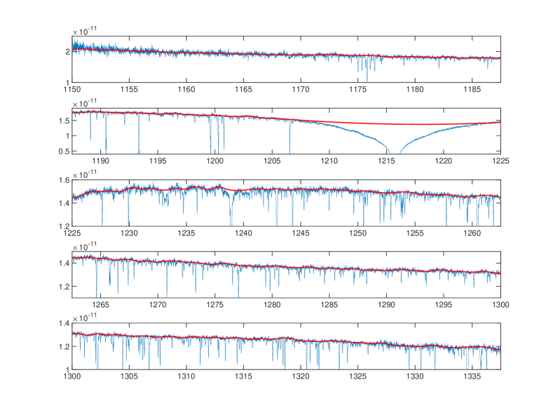
Figure 3: G191$-$B2B continuum model with 0.75 Å knot spacing.

Using these four continua, we then detect absorption lines which are significant at or above 5$\sigma$ (see Table 1). This number of lines identified at or above this significance limit, in the range 1150 Å to 1894 Å, for each of the four knot spacings, is also given in Table 1). Using custom Python code, the observed feature wavelengths were then shifted to the rest-frame using a G191$-$B2B redshift of 23.8 $\pm$ 0.03 km s^-1 from Preval et al. (2013)). The rest-frame wavelengths were then matched to recently updated Ni v laboratory wavelengths (provided as online supplementary material), where a match was accepted for agreement equal to or better than 3$\sigma$, allowing for both observational and laboratory wavelength uncertainties. For each knot spacing, a total of 299, 316, 325 and 320 potential Ni v matches were made respectively, of which 258, 270, 281 and 278 have associated $q$-coefficients (see Table 1). However, as can be seen in Table D, there are many cases where multiple identifications are possible. All multiple IDs are removed from the linear regression procedure to measure $\Delta\alpha/\alpha$. Finally, a visual inspection of Figure 3 shows that there are a few spectral regions that need to be avoided: [1205, 1227], [1238,1241], [1242,1243.5], [1345,1347] Å. All Ni v transition within these 4 windows are discarded.

Having identified the lines to be used, we follow a similar procedure to that used in Berengut et al. (2013). The observed-frame wavelength $\lambda_{obs,i}$ of the $i^{th}$ absorption line in the white dwarf photosphere, and the corresponding rest-frame laboratory wavelength $\lambda_{0,i}$, are related by

$$\frac{\lambda_{obs,i}-\lambda_{0,i}}{\lambda_{0,i}}=\frac{\Delta\lambda_{i}}{\lambda_{0,i}} =z-\frac{2q_{i}\lambda_{obs,i}}{10^{8}}\frac{\Delta\alpha}{\alpha_{0}}$$

$$=z-Q_{i}\frac{\Delta\alpha}{\alpha_{0}}$$ (24)

where wavelengths are in Å, $q_{i}$ (in cm^-1) is the relative sensitivity of the transition frequency to variation in $\alpha$, $z$ is the white dwarf redshift (comprising gravitational and kinematic contributions), and $\Delta\alpha/\alpha=(\alpha_{WD}-\alpha_{0})/\alpha_{0}$.

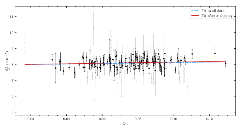
Figure 4: Eq. (24) for one example trial continuum (0.75Å knot spacing). Grey points were removed when $\sigma$-clipping was applied. See Section 5 for details.

Knot spacing (Å)	0.5	0.75	1.0	1.25
5$\sigma$ detections	1566	1678	1789	1752
NiV matches total	299	316	325	320
NiV matches having q (no $\sigma$-clipping)	167	165	163	164
$\Delta\alpha/\alpha\times 10^{-5}$	$-1.530\pm 1.101$	$-1.462\pm 1.121$	$-1.624\pm 1.156$	$-1.980\pm 1.150$
$z\times 10^{-5}$	$7.957\pm 0.085$	$7.962\pm 0.087$	$7.940\pm 0.090$	$7.920\pm 0.090$
$\chi^{2}_{\nu}$	1.950	1.869	1.943	1.918
NiV matches having q (after $\sigma$-clipping)	125	128	125	127
$\Delta\alpha/\alpha\times 10^{-5}$	$-2.153\pm 1.193$	$-1.771\pm 1.187$	$-2.856\pm 1.229$	$-2.625\pm 1.215$
$z\times 10^{-5}$	$7.955\pm 0.092$	$7.968\pm 0.092$	$7.888\pm 0.095$	$7.906\pm 0.095$
$\chi^{2}_{\nu}$	0.995	0.980	0.982	0.997

Table 1: The impact of using different white dwarf continuum models on measurements of $\Delta\alpha/\alpha$. Four model continua, each corresponding to a different knot spacing. The results show that the additional uncertainty on $\Delta\alpha/\alpha$ associated by continuum placement variation is comparable to or even larger than the statistical uncertainty. The first row gives the total number of 5$\sigma$ NiV detections in the HST STIS spectrum. The second row shows the total number of lines identified as potential NiV, matched within 3$\sigma$ of the Ward et al. laboratory list (allowing for the white dwarf redshift), including multiple potential IDs. Where more than 1 possible match exists (see Appendix D), we discard that line entirely from further analysis. Observed and laboratory wavelength matches were made using the newly calculated Ni v $q$-coefficients and the Ward et al. (2019) Ni v laboratory wavelengths updated as part of this work by A. Kramida. The second block in the table shows measurements for all lines that have $q$ coefficient calculations (given in Appendix C). The third block shows the same thing as the second block, except deviant points (measured in units of $\sigma$) were iteratively clipped during linear regression until $\chi^{2}_{\nu}\leq 1$. $\chi^{2}_{\nu}$ is defined by Eq.(25). The other continuum fitting parameter settings are: smoothing FWHM $3\bar{x}$ (Section 3.1), $\zeta=3$ (Section 3.2), $k_{merge}=1/3$ (Section 3.3), $n=10$ (Section 3.7).

A linear regression analysis on the matched Ni v lines is then used to solve for the parameters $z$ and $\Delta\alpha/\alpha$, for each of the four model continua. The results of this are given in Table 1 and, for one example knot spacing, illustrated in Figure 4 (details for all knot spacings are given in the Supplementary Material. The table also gives the reduced chi-squared, which in this case is

$$\chi^{2}_{\nu}=\frac{1}{N-2}\sum_{i=1}^{N}\left(\frac{y_{i}-(\Delta\lambda/\lambda_{0})_{i}}{\sigma(\Delta\lambda/\lambda_{0})_{i})}\right)^{2}$$ (25)

Clearly, the $\chi^{2}_{\nu}$ values are larger than the expected value of unity for a good fit to the data. This is unsurprising: the scatter in the “continuum” points fitted will be increased by the presence of weak unidentified absorption lines that were not detected using the 5$\sigma$ detection threshold. Further, the continuum model is likely to be inadequate in places for the instrumental/data processing reasons explained previously.

5.1 Potential bias

The impact of assuming $\Delta\alpha/\alpha=0$ when matching laboratory and white dwarf lines was discussed in Hu et al. (2021) (see section 5.2 and figure 2 in that paper). That numerical experiment was carried out using Fe v, altering the input assumption multiple times, using a range $\Delta\alpha/\alpha=\pm 10^{3}$, in steps of $\Delta\alpha/\alpha=10^{-5}$. No evidence was seen for bias in the Hu et al. (2021) analysis. Nevertheless, it should not necessarily be assumed that there is no bias in the analysis carried out here using Ni v. It is possible that the assumption of $\Delta\alpha/\alpha=0$ when performing line identifications may result in some fraction of false identifications, potentially biasing the slope in Fig. 4. However, our focus in this paper is to explore the impact of continuum placement. A detailed study of this kind of bias, in the sense described above, is beyond the scope of the present work, but we note the potential issue here to motivate explicit checks in future measurements.

6 Discussion and future work

In this work we have developed a new algorithm for continuum fitting high resolution spectra. The method is automated, reproducible, and objective. Here we have applied it to a high-resolution, high signal-to-noise HST/STIS spectrum of the white dwarf G191$-$B2B. In a companion article we apply it to quasar spectroscopy. Using this algorithm we obtained four different estimates for the underlying G191$-$B2B continuum in order to examine the impact of continuum placement uncertainties on measurements of the fine structure constant in the strong gravitational field at the G191$-$B2B photosphere.

An earlier analysis (Berengut et al., 2013) found anomalous results when comparing $\Delta\alpha/\alpha$ measurements derived using Fe v and Ni v transitions detected in the G191$-$B2B photosphere. We draw attention to figure 1 in that paper, where different slopes were found using the linear relationship expressed in Eq.(24); they found $\Delta\alpha/\alpha=(4.2\pm 1.6)\times 10^{-5}$ and $(-6.1\pm 5.8)\times 10^{-5}$ for Fe v and Ni v respectively. The interpretation suggested in (Berengut et al., 2013) was that systematics were present in the available Ni v laboratory wavelength measurements.

More recently, Hu et al. (2021) carried out a more detailed analysis using Fe v transitions, using the same astronomical data. The best result found by Hu et al. (2021) is $\Delta\alpha/\alpha=(6.36\pm 0.35_{stat}\pm 1.84_{sys})\times 10^{-5}$, consistent with the earlier Fe v result from Berengut et al. (2013).

New, independent Ni v laboratory wavelength measurements have been made (Ward et al., 2019). Also, new sensitivity coefficient ($q$) calculations have been carried out and reported in this paper (Appendix C). These new data thus allow us to re-examine the apparent Fe v/Ni v inconsistency previously reported. Comparing the best available Fe v measurement (Hu et al., 2021) with the most positive result obtained in the present work (no $\sigma$-clipping, 0.75Å knot spacing, see Table 1), a significant (3.2$\sigma$) discrepancy remains (more significant if we take any of the other Ni v measurements obtained in the present work).

Our main results from this work therefore are:

1. Slight changes in the underlying continuum can impact on $\Delta\alpha/\alpha$ measurements, as illustrated in Table 1; the additional uncertainty on $\Delta\alpha/\alpha$ associated with continuum placement variations is not negligible compared to the statistical (i.e. covariance matrix) uncertainty on $\Delta\alpha/\alpha$.

2. Curiously, the $\Delta\alpha/\alpha$ measurements we have made, using entirely independent Ni v laboratory wavelengths and new $q$ coefficients, are still of opposite sign to the Fe v measurements reported in both Berengut et al. (2013) and Hu et al. (2021). The explanation for this continuing significant discrepancy has yet to be found.

There is an important caveat to the first result listed above: the analysis in the present work is based on absorption line centroiding and linear regression method, as for Berengut et al. (2013). A different approach is that of Hu et al. (2021), in which absorption lines are modelled using Voigt profiles. In the latter, the fits to local continuum segments can be refined using additional free parameters included in the non-linear least squares fitting procedure (see Carswell & Webb 2023 for details). That process may substantially reduce the error contribution found here. We have not explored this here for white dwarf spectroscopy, although a companion paper to this one, describing the analysis of the spectrum of quasar PHL957, suggests local continuum refinement dramatically reduces the impact of variations in the initial continuum model.

The results presented in this paper have important implications for the claimed uncertainties in some previous published $\Delta\alpha/\alpha$ measurements, including the recent measurements of, for example, Hees et al. (2020); Murphy et al. (2022). There are likely to also be significant implications for the achievable precision in forthcoming redshift drift studies (Sandage, 1962; Liske et al., 2008); the results reported here motivate a more careful exploration of the potential systematics that may arise from continuum estimation across the Lyman alpha forest.

Data Availability

Based on observations made with the NASA/ESA Hubble Space Telescope, obtained from the data archive at the Space Telescope Science Institute. The STIS spectra of G191$-$B2B are available from the Barbara A. Mikulski archive. The continuum fitting code described in this paper is available from the authors on request.

Appendix A Solving for $\Delta\alpha/\alpha$ using linear regression

Let $x=(\alpha/\alpha_{0})^{2}-1$. For the $i^{th}$ absorption line,

$$\omega_{rest,i}=\omega_{0,i}+q_{i}x$$ (26)

where $\omega_{rest,i}$ is the observed rest-frame frequency of the $i^{th}$ line measured in the white dwarf spectrum (i.e. $\omega_{rest,i}$ does not include the white dwarf redshift, the combined effects of gravitational redshift and line of sight stellar velocity). $\omega_{0,i}$ is the terrestrial laboratory rest-frame frequency. $q_{i}$ is the sensitivity coefficient for that line. $\omega$ and $q$ are both in units of cm^-1. The observed-frame and rest-frame frequencies of the $i^{th}$ line measured in the white dwarf spectrum are related by

$$\omega_{rest,i}=\omega_{obs,i}(1+z)$$ (27)

so Eq. 26 becomes

$$\omega_{obs,i}+z\omega_{obs,i}=\omega_{0,i}+q_{i}x$$ (28)

Using the approximation $x\approx 2\Delta\alpha/\alpha_{0}$, where $\Delta\alpha=\alpha-\alpha_{0}$, Eq. 28 becomes

$$\omega_{obs,i}-\omega_{0,i}=-z\omega_{obs,i}+2q_{i}\frac{\Delta\alpha}{\alpha_{0}}$$ (29)

so

$$\frac{\omega_{obs,i}-\omega_{0,i}}{\omega_{obs,i}}=-z+\frac{2q_{i}}{\omega_{obs,i}}\frac{\Delta\alpha}{\alpha_{0}}$$ (30)

and with $\lambda$ in Å, $\omega=10^{8}/\lambda$,

$$\frac{\lambda_{obs,i}-\lambda_{0,i}}{\lambda_{0,i}}=\frac{\Delta\lambda_{i}}{\lambda_{0,i}}=z-\frac{2q_{i}\lambda_{obs,i}}{10^{8}}\frac{\Delta\alpha}{\alpha_{0}}$$ (31)

The version of Eq. 31 used in Berengut et al 2013 is,

$$\frac{\Delta\lambda_{i}}{\lambda_{0,i}}=z-\frac{2q_{i}\lambda_{0,i}}{10^{8}}(1+z)\frac{\Delta\alpha}{\alpha_{0}}.$$ (32)

Eq. 32 thus assumes $\lambda_{obs,i}/\lambda_{0,i}=(1+z)$, which is correct if $\Delta\alpha/\alpha_{0}=0$, but an approximation otherwise. The exact expression is $\lambda_{obs,i}/\lambda_{rest,i}=(1+z_{i})$. Whilst both equations give very close results ($\Delta\alpha/\alpha$ discrepancies are at the $10^{-8}$ level, well below any realistic experimental error), in this work we use Eq. 31 to solve for the slope and intercept $\Delta\alpha/\alpha$ and $z$.

Appendix B Complete set of figures

In the main paper we illustrate only one continuum (0.75Å knot spacing). Here we illustrate the complete set used in these measurements, i.e. continua computed for all four knot spacings: 0.5, 0.75, 1.0, 1.25Å.

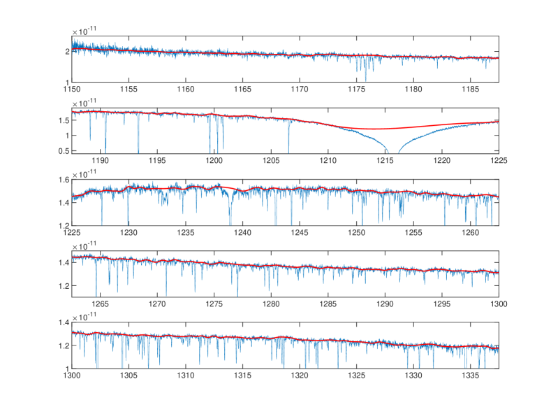
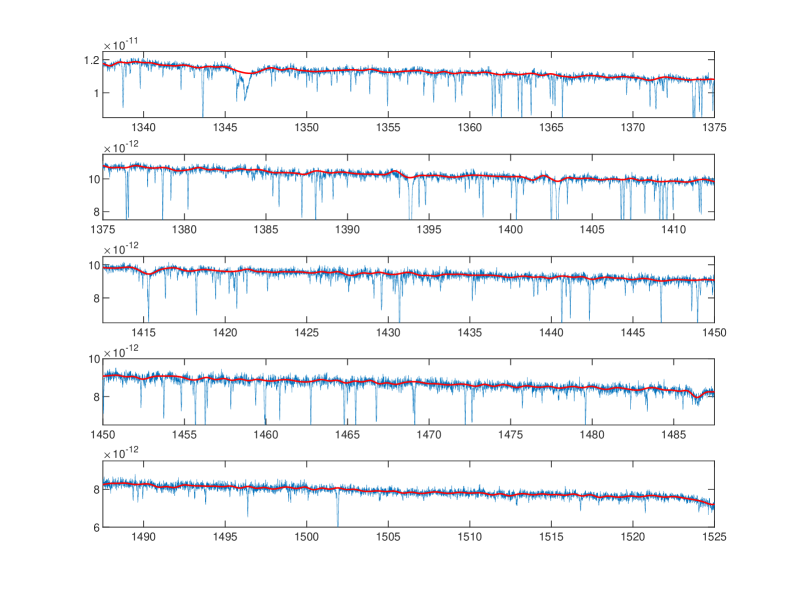
Figure 5: G191$-$B2B continuum model with 0.5 Å knot spacing.

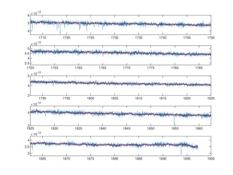
Figure 6: G191$-$B2B continuum model with 0.5 Å knot spacing.

Figure 7: G191$-$B2B continuum model with 0.75 Å knot spacing.

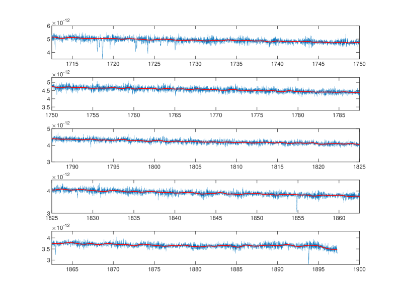
Figure 8: G191$-$B2B continuum model with 0.75 Å knot spacing.

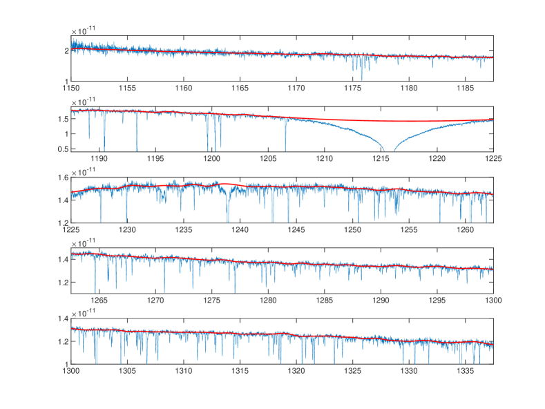
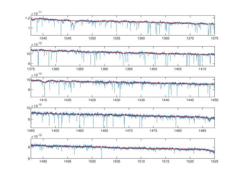
Figure 9: G191$-$B2B continuum model with 1.0 Å knot spacing.

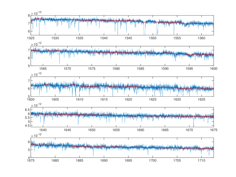
Figure 10: G191$-$B2B continuum model with 1.0 Å knot spacing.

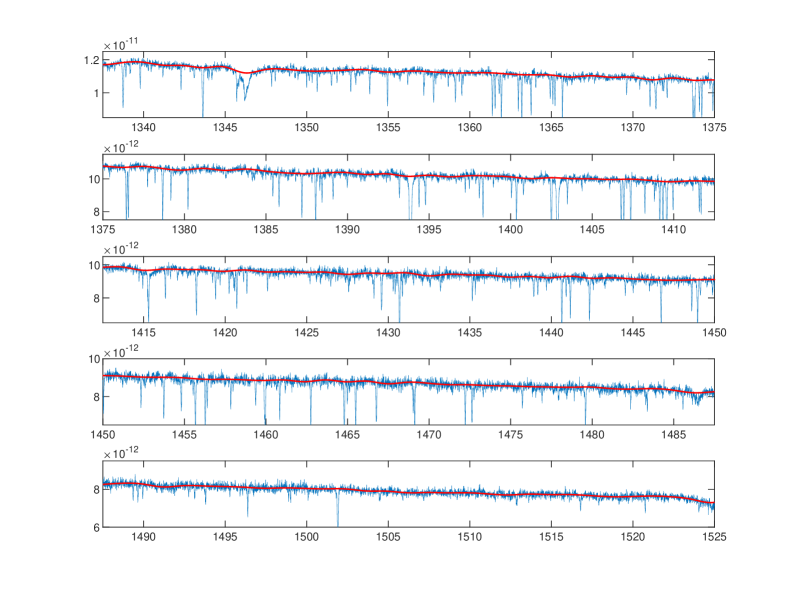
Figure 11: G191$-$B2B continuum model with 1.25 Å knot spacing.

Figure 12: G191$-$B2B continuum model with 1.25 Å knot spacing.

Appendix C Atomic data NiV

Experimental and theoretical data on energy levels of Ni V. For further details about the experimental data see Kramida et al. (2022). Apart from the energies, the theoretical data include calculated Landé $g$-factors and sensitivity coefficients $q$. The atomic data provided here for NiV is analogous to similar files for FeV provided as supplementary material in Hu et al. (2021). For enquiries about the theoretical data, contact Vladimir Dzuba: v.dzuba@unsw.edu.au.

Table 2: Even energy levels.

Experimental data				Theoretical data
Configuration	Term	$J$	Energy	Energy	$g$	$q$
			[cm-1]	[cm-1]		[cm-1]
3d6()	5D	0	2057.6	1396	0.0000	1829
3d6()	3P2	0	29640.0	34626	0.0000	2557
3d6()	1S2	0	47699.7	51554	0.0000	1487
3d6()	3P1	0	66737.8	73326	0.0000	-940
3d6()		0		148275	0.0000	324
3d5.(4D).4s	5D	0	216305.7	211486	0.0000	-6971
		0		215959	0.0000	-6250
		0		259128	0.0000	-6666
		0		302100	0.0000	-6966
3d6()	5D	1	1871.5	2516	1.4998	1691
3d6()	3P2	1	28697.6	34535	1.4962	2209
3d6()	3D	1	41701.1	46758	0.5049	629
3d6()	3P1	1	67547.9	74931	1.4991	-168
3d5.(4P).4s	5P	1	212455.7	207163	2.4590	-7116
3d5.(4D).4s	5D	1	216434.7	211590	1.5371	-6657
3d5.(4P).4s	3P	1	221429.0	215767	1.4491	-6758
3d5.(4D).4s	3D	1	225545.1	220256	0.5474	-6088
3d5.(2D3).4s	3D	1	232910.8	229753	0.2174	-7827
3d5.(4F).4s	5F	1	235116.5	232189	0.2897	-5611
3d5.(2S).4s	3S	1	253905.2	254966	1.9996	-6825
3d5.(2D2).4s	3D	1	263700.9	264761	0.5003	-6878
3d5.(2D1).4s	3D	1	307105.1	302035	1.4955	-7063
		1		306249	0.9939	-7038
		1		313495	0.5112	-6765
3d6()	5D	2	1489.9	1790	1.4995	1382
3d6()	3P2	2	26153.0	30208	1.4965	-425
3d6()	3F2	2	29899.2	33189	0.6701	933
3d6()	3D	2	41626.9	45802	1.1653	433
3d6()	1D2	2	48607.0	56120	1.0043	1085
3d6()	3F1	2	68632.1	74836	0.6698	542
3d6()	3P1	2	69156.1	76951	1.4946	1648
3d6()	1D1	2	104420.5	114888	0.9999	460
3d5.(6S).4s	5S	2	178019.8	165585	1.9991	-6212
3d5.(4G).4s	5G	2	208151.5	200680	0.3353	-7018
3d5.(4P).4s	5P	2	212253.4	206958	1.8033	-7509
3d5.(4D).4s	5D	2	216590.5	211742	1.5257	-6305
3d5.(4P).4s	3P	2	221087.6	215453	1.4642	-7412
3d5.(4D).4s	3D	2	225616.5	220456	1.1951	-5872
3d5.(2D3).4s	3D	2	232655.6	229615	1.0277	-8247
3d5.(4F).4s	5F	2	234412.7	231112	0.9074	-7170
3d5.(2F1).4s	3F	2	235736.5	232870	0.9695	-6243
3d5.(2D3).4s	1D	2	239107.7	236370	0.9117	-4938
3d5.(4F).4s	3F	2	243266.2	239538	0.6925	-6121
3d5.(2F2).4s	3F	2	247165.0	245934	0.6697	-6562
3d5.(2D2).4s	3D	2	263735.7	265044	1.1658	-6783
3d5.(2D2).4s	1D	2	268273.9	269325	0.9996	-6576
3d5.(2D1).4s	3D	2	307025.2	302060	1.4971	-7180
3d5.(2D1).4s	1D	2	311470.3	313629	1.1682	-6917
		2		317855	1.0012	-6809
3d6()	5D	3	889.7	1250	1.4992	896
3d6()	3F2	3	29570.8	33285	1.0622	505
3d6()	3G	3	34416.4	37773	0.7727	1769
3d6()	3D	3	41920.2	46657	1.3319	848
3d6()	1F	3	57924.1	64500	1.0033	293
3d6()	3F1	3	68854.7	75646	1.0806	1183
3d5.(6S).4s	7S	3	164525.9	152772	1.9995	-6678
3d5.(4G).4s	5G	3	208164.6	200761	0.9175	-6922
3d5.(4P).4s	5P	3	212095.8	206908	1.6488	-7762
3d5.(4D).4s	5D	3	216596.0	209293	0.7523	-6702
3d5.(4G).4s	3G	3	217101.0	211921	1.5126	-6230
3d5.(4D).4s	3D	3	225200.7	219960	1.3318	-6610
3d5.(2D3).4s	3D	3	232545.9	229644	1.2580	-8398
3d5.(4F).4s	5F	3	234275.2	230996	1.2337	-6944
3d5.(2F1).4s	3F	3	236454.1	233743	1.1427	-5430
3d5.(2F1).4s	1F	3	240193.8	237218	1.0167	-5882
3d5.(2G2).4s	3G	3	242290.4	239187	0.9910	-6611
3d5.(4F).4s	3F	3	243370.5	240142	0.8601	-6183
3d5.(2F2).4s	3F	3	247104.9	245961	1.0846	-6647
3d5.(2F2).4s	1F	3	251654.9	250168	1.0023	-6475
3d5.(2D2).4s	3D	3	263805.8	265275	1.3313	-6590
3d5.(2G1).4s	3G	3	274773.5	276114	0.7506	-6784
3d5.(2D1).4s	3D	3	306962.9	313547	1.3333	-7018
3d6()	5D	4	0.0	-0	1.4988	0
3d6()	3H	4	27858.8	30010	0.8318	387
3d6()	3F2	4	29123.7	32475	1.2046	183
3d6()	3G	4	34061.7	36822	1.0612	1600
3d6()	1G2	4	42208.1	45917	1.0037	1454
3d6()	3F1	4	68718.7	74766	1.2476	636
3d6()	1G1	4	77899.5	85539	1.0023	773
3d5.(4G).4s	5G	4	208163.7	200835	1.1503	-6829
3d5.(4D).4s	5D	4	216189.9	209318	1.0509	-6518
3d5.(4G).4s	3G	4	217129.1	211531	1.4982	-6927
3d5.(4F).4s	5F	4	234125.4	230800	1.3452	-7025
3d5.(2F1).4s	3F	4	235420.6	232594	1.2505	-6581
3d5.(2H).4s	3H	4	240959.6	236976	0.8335	-7430
3d5.(2G2).4s	3G	4	242504.3	238958	1.1901	-6927
3d5.(4F).4s	3F	4	243331.5	240278	1.0715	-6057
3d5.(2G2).4s	1G	4	247049.1	244341	1.0094	-5918
3d5.(2F2).4s	3F	4	247281.8	245917	1.2503	-6592
3d5.(2G1).4s	3G	4	274738.6	276093	1.0501	-6822
3d5.(2G1).4s	1G	4	279199.5	280311	1.0002	-6684
3d6 ()	3H	5	27578.2	29506	1.0404	503
3d6 ()	3G	5	33256.5	36405	1.1929	768
3d5.(4G).4s	5G	5	208131.0	200830	1.2666	-6770
3d5.(4G).4s	3G	5	217048.7	209359	1.1996	-6483
3d5.(2I).4s	3I	5	229413.0	222780	0.8355	-7026
3d5.(4F).4s	5F	5	234082.1	230750	1.3953	-7077
3d5.(2H).4s	3H	5	241082.2	237200	1.0521	-7095
3d5.(2G2).4s	3G	5	242862.6	239964	1.1575	-6323
3d5.(2H).4s	1H	5	246240.9	242144	1.0268	-5814
3d5.(2G1).4s	3G	5	274695.4	276128	1.2000	-6866
3d6()	3H	6	27111.2	28827	1.1653	279
3d6()	1I	6	41252.2	43790	1.0014	945
3d5.(4G).4s	5G	6	208046.4	200881	1.3330	-6792
3d5.(2I).4s	3I	6	229408.8	222883	1.0250	-6908
3d5.(2I).4s	1I	6	233839.2	227172	1.0021	-6762
3d5.(2H).4s	3H	6	241773.6	237776	1.1638	-6164

Table 3: Odd energy levels.

Experimental data				Theoretical data
Configuration	Term	$J$	Energy	Energy	$g$	$q$
			[cm-1]	[cm-1]		[cm-1]
3d5.(4P).4p	5D*	0	290262.0	281464	0.0000	-5470
3d5.(4P).4p	3P*	0	293867.0	287790	0.0000	-3601
3d5.(4D).4p	5D*	0	298060.0	291969	0.0000	-2663
3d5.(4D).4p	3P*	0	305386.9	299362	0.0000	-4301
3d5.(2D3).4p	3P*	0	313577.3	309703	0.0000	-3418
3d5.(4F).4p	5D*	0	317462.3	313175	0.0000	-2326
3d5.(2S).4p	3P*	0	329618.5	329372	0.0000	-5126
3d5.(2D2).4p	3P*	0	346920.2	347460	0.0000	-3490
3d5.(2P).4p	3P*	0	368440.5	373470	0.0000	-4946
				378828	0.0000	-3974
				399017	0.0000	-2695
3d5.(6S).4p	5P*	1	254885.0	241377	2.4987	-2708
3d5.(4P).4p	5D*	1	287755.5	280878	0.2950	-3976
3d5.(4G).4p	5F*	1	289163.0	281723	1.1991	-4762
3d5.(4P).4p	5P*	1	291541.7	285184	2.3645	-3997
3d5.(4P).4p	3P*	1	293420.0	287310	1.4579	-3978
3d5.(4D).4p	5F*	1	293833.8	287628	0.1650	-4603
3d5.(4D).4p	5D*	1	297417.9	291341	1.3386	-3715
3d5.(4D).4p	5P*	1	297982.8	291883	1.1669	-3649
3d5.(4P).4p	*	1	298600.6	292692	1.9791	-3134
3d5.(4D).4p	3D*	1	300563.3	294473	0.5265	-2497
3d5.(4P).4p	3S*	1	303249.5	296357	1.9601	-3800
3d5.(4D).4p	3P*	1	305838.1	299924	1.5284	-3576
3d5.(2D3).4p	*	1	312291.0	308444	0.9373	-5157
3d5.(2D3).4p	*	1	313679.0	309782	0.8141	-3762
3d5.(4F).4p	5F*	1	315152.8	310866	0.3252	-3727
3d5.(2F1).4p	3D*	1	315300.7	311524	0.7944	-4032
3d5.(4F).4p	5D*	1	317477.9	313240	1.2865	-2263
3d5.(2D3).4p	1P*	1	319073.4	315355	0.8106	-1346
3d5.(4F).4p	3D*	1	322984.5	318413	0.5500	-2697
3d5.(2F2).4p	3D*	1	329462.3	326703	0.5249	-3574
3d5.(2S).4p	3P*	1	330370.7	329930	1.4656	-4581
3d5.(2S).4p	1P*	1	334477.2	334712	1.0120	-3450
3d5.(2D2).4p	3D*	1	343478.2	343245	0.5459	-4549
3d5.(2D2).4p	3P*	1	346959.5	347592	1.4304	-3410
3d5.(2D2).4p	1P*	1	348477.9	348816	1.0233	-3251
3d5.(2P).4p	3P*	1	368749.7	373807	1.5033	-4797
3d5.(2P).4p	3D*	1	374828.1	379609	0.5133	-5064
3d5.(2P).4p	3S*	1	378555.0	383711	1.6646	-3986
3d5.(2P).4p	1P*	1	380165.6	384557	1.3169	-3363
3d5.(2D1).4p	3D*	1	388746.1	394103	0.5120	-4887
				398508	1.4944	-3300
				404010	0.9956	-3522
3d5.(6S).4p	5P*	2	254495.6	229894	2.3277	-4828
3d5.(4G).4p	5G*	2	284215.5	241014	1.8375	-3014
3d5.(4P).4p	5D*	2	287782.1	276075	0.3521	-4786
3d5.(4P).4p	*	2	288877.9	280657	1.0598	-4086
3d5.(4G).4p	5F*	2	289247.1	282019	1.4292	-4927
3d5.(4G).4p	3F*	2	291097.7	282941	0.9106	-4043
3d5.(4P).4p	5P*	2	291390.0	283078	1.6798	-4724
3d5.(4P).4p	3P*	2	292983.0	285114	1.7959	-3535
3d5.(4D).4p	5F*	2	294086.0	286909	1.5530	-4015
3d5.(4D).4p	5D*	2	297013.9	287948	1.0263	-4325
3d5.(4P).4p	3D*	2	297842.5	290869	1.4007	-4204
3d5.(4D).4p	5P*	2	299045.6	291690	1.3451	-3841
3d5.(4D).4p	3D*	2	300224.9	293244	1.6688	-2780
3d5.(4D).4p	3F*	2	301553.0	294134	1.2039	-2872
3d5.(4D).4p	3P*	2	306377.8	295583	0.7273	-2664
3d5.(2D3).4p	3F*	2	307731.1	300678	1.4975	-3224
3d5.(2D3).4p	*	2	308943.0	303830	0.7770	-5966
3d5.(2D3).4p	3P*	2	311966.5	305575	0.9302	-5128
3d5.(4F).4p	5G*	2	312778.2	307992	0.7962	-5100
3d5.(2D3).4p	3D*	2	313686.6	308407	0.9480	-4171
3d5.(4F).4p	5F*	2	314834.7	309715	1.0745	-4288
3d5.(2F1).4p	*	2	315366.1	310696	1.1579	-3761
3d5.(2F1).4p	*	2	316165.4	311537	0.7948	-2882
3d5.(4F).4p	5D*	2	317517.5	312447	1.2081	-2480
3d5.(2F1).4p	1D*	2	319926.5	313434	1.3131	-1661
3d5.(2G2).4p	3F*	2	321018.3	316167	0.9754	-3391
3d5.(4F).4p	3D*	2	322436.4	317360	0.7783	-3505
3d5.(4F).4p	3F*	2	323853.1	318193	1.0621	-3368
3d5.(2F2).4p	3F*	2	325982.2	319793	0.6943	-2601
3d5.(2F2).4p	1D*	2	327122.7	323571	0.7952	-4036
3d5.(2F2).4p	3D*	2	329776.3	325064	0.8932	-2819
3d5.(2S).4p	3P*	2	331678.2	326810	1.1605	-3332
3d5.(2D2).4p	3F*	2	342894.6	331480	1.4933	-2963
3d5.(2D2).4p	3D*	2	343905.7	342876	0.7859	-5049
3d5.(2D2).4p	3P*	2	346912.4	343840	1.0749	-4135
3d5.(2D2).4p	1D*	2	349546.0	347523	1.4455	-3437
3d5.(2G1).4p	3F*	2	355150.0	349161	1.0256	-3122
3d5.(2P).4p	3P*	2	369649.1	355824	0.6675	-2843
3d5.(2P).4p	3D*	2	374803.7	374877	1.4917	-3844
3d5.(2P).4p	1D*	2	377059.1	379589	1.1140	-5230
3d5.(2D1).4p	3F*	2	386968.8	382070	1.0570	-3051
3d5.(2D1).4p	3D*	2	389571.8	392115	0.7063	-5044
3d5.(2D1).4p	1D*	2	390675.1	395085	1.1438	-3946
3d5.(2D1).4p	3P*	2	392413.5	396028	1.0955	-4338
3d5.(6S).5p	5P*	2	423782	397840	1.3919	-3591
3d5.(6S).4p	7P*	3	243608.5	230698	1.9118	-4119
3d5.(6S).4p	5P*	3	253862.7	240404	1.6705	-3569
3d5.(4G).4p	5G*	3	284249.0	276109	0.8765	-4826
3d5.(4G).4p	5H*	3	286293.6	277563	0.5556	-4806
3d5.(4G).4p	*	3	287960.0	280438	1.2565	-4072
3d5.(4G).4p	5F*	3	289298.0	282481	1.4906	-4859
3d5.(4P).4p	5P*	3	290757.0	283221	1.0889	-3425
3d5.(4G).4p	3F*	3	291328.5	284588	1.6263	-3939
3d5.(4D).4p	5F*	3	294443.3	288126	0.7528	-3554
3d5.(4D).4p	5D*	3	296574.0	288491	1.2649	-3921
3d5.(4G).4p	3G*	3	296847.1	290332	1.4271	-4843
3d5.(4P).4p	3D*	3	297418.1	291221	1.4131	-4357
3d5.(4D).4p	3D*	3	298972.3	293092	1.4568	-3460
3d5.(4D).4p	*	3	300201.0	294296	1.4822	-2654
3d5.(4D).4p	3F*	3	301470.2	295588	1.1320	-2604
3d5.(2D3).4p	3F*	3	308592.0	304514	1.0407	-5969
3d5.(2F1).4p	3G*	3	312463.3	308099	0.9539	-5016
3d5.(4F).4p	5G*	3	312889.4	308350	0.8926	-4790
3d5.(2F1).4p	*	3	312953.6	309183	1.2718	-4865
3d5.(2F1).4p	*	3	313919.8	310109	1.3019	-4626
3d5.(4F).4p	5F*	3	314562.8	310586	1.2231	-4363
3d5.(2F1).4p	*	3	315326.2	311337	0.9816	-2939
3d5.(2F1).4p	*	3	316280.3	312453	1.0733	-2638
3d5.(4F).4p	5D*	3	317232.0	312947	1.1158	-2667
3d5.(4F).4p	*	3	317376.8	313303	1.1083	-1828
3d5.(4F).4p	3G*	3	319620.2	315318	0.7914	-3194
3d5.(2G2).4p	3F*	3	320513.8	316580	1.0024	-3333
3d5.(2F1).4p	1F*	3	321081.9	317033	1.1152	-3815
3d5.(4F).4p	3D*	3	322617.6	318370	1.2656	-3181
3d5.(4F).4p	3F*	3	323532.2	319057	1.0834	-3476
3d5.(2G2).4p	3G*	3	325211.9	321602	0.7825	-2976
3d5.(2F2).4p	3F*	3	326029.9	323176	1.0058	-2709
3d5.(2G2).4p	1F*	3	326739.0	323938	1.0686	-3747
3d5.(2F2).4p	3G*	3	329614.3	326076	0.8248	-4116
3d5.(2F2).4p	3D*	3	329872.9	326723	1.2729	-3339
3d5.(2F2).4p	1F*	3	334727.6	332526	1.0048	-3182
3d5.(2D2).4p	3F*	3	343281.0	343388	1.1491	-4646
3d5.(2D2).4p	3D*	3	344805.3	344753	1.2438	-2962
3d5.(2D2).4p	1F*	3	345936.1	346185	1.0196	-3164
3d5.(2G1).4p	3F*	3	353944.1	354411	0.9271	-4699
3d5.(2G1).4p	3G*	3	355398.0	355868	0.9137	-3176
3d5.(2G1).4p	1F*	3	360059.7	360180	0.9941	-3387
3d5.(2P).4p	3D*	3	376471.6	381384	1.3320	-3382
3d5.(2D1).4p	3F*	3	387333.4	392545	1.1028	-4947
3d5.(2D1).4p	3D*	3	390478.2	396043	1.3067	-2888
3d5.(2D1).4p	1F*	3	392957.1	397826	1.0084	-3427
3d5.(6S).4p	7P*	4	244900.5	231980	1.7496	-2661
3d5.(4G).4p	5G*	4	284308.9	276164	1.1113	-4773
3d5.(4G).4p	5H*	4	286706.6	278070	0.9487	-4203
3d5.(4G).4p	5F*	4	288161.6	280235	1.3385	-3939
3d5.(4G).4p	3F*	4	291554.6	283505	1.2629	-3200
3d5.(4G).4p	3H*	4	292631.0	283699	0.8043	-3264
3d5.(4D).4p	5F*	4	294939.6	284038	1.4715	-3334
3d5.(4G).4p	3G*	4	296897.0	288262	1.0531	-3357
3d5.(4D).4p	5D*	4	296919.3	289118	1.3559	-3330
3d5.(4D).4p	3F*	4	300918.1	290810	1.4875	-4232
3d5.(2I).4p	3H*	4	309952.5	295022	1.2618	-3416
3d5.(2D3).4p	3F*	4	310212.6	302913	0.8060	-3389
3d5.(2F1).4p	1G*	4	312008.3	306255	1.2059	-4108
3d5.(4F).4p	5G*	4	313281.3	308059	1.0640	-4996
3d5.(2F1).4p	*	4	314208.8	308751	1.1121	-4469
3d5.(4F).4p	5F*	4	314599.2	309768	1.2790	-4390
3d5.(2G2).4p	3H*	4	315370.1	310292	1.2267	-3672
3d5.(2D3).4p	*	4	316068.8	310978	0.8805	-4816
3d5.(4F).4p	5D*	4	316744.0	311935	1.0965	-2639
3d5.(2H).4p	*	4	316887.8	312339	1.4220	-3314
3d5.(2G2).4p	*	4	319138.7	312830	1.0755	-2983
3d5.(4F).4p	3G*	4	319899.1	315218	1.0526	-3272
3d5.(2G2).4p	3F*	4	321056.4	315252	1.0822	-3461
3d5.(4F).4p	3F*	4	322820.8	317653	1.1721	-2969
3d5.(2H).4p	3H*	4	323926.3	318562	1.2436	-3761
3d5.(2G2).4p	3G*	4	325222.9	319411	0.8302	-3839
3d5.(2F2).4p	*	4	325558.6	321537	1.0597	-2853
3d5.(2F2).4p	3F*	4	326876.3	321989	1.0144	-3604
3d5.(2F2).4p	3G*	4	330297.6	324418	1.2174	-3042
3d5.(2H).4p	1G*	4	332995.6	326849	1.0624	-3158
3d5.(2D2).4p	3F*	4	344911.2	329270	1.0025	-3365
3d5.(2G1).4p	3H*	4	353071.6	345121	1.2487	-2780
3d5.(2G1).4p	3F*	4	353347.1	353117	0.8394	-5094
3d5.(2G1).4p	3G*	4	355765.2	353776	1.1998	-4993
3d5.(2G1).4p	1G*	4	358760.0	356094	1.0564	-3153
3d5.(2D1).4p	3F*	4	388698.9	358898	1.0052	-3293
		4		393842	1.2500	-3205
3d5.(4G).4p	5G*	5	284402.5	276314	1.2360	-4635
3d5.(4G).4p	5H*	5	287127.2	278555	1.1406	-3702
3d5.(4G).4p	5F*	5	287906.9	279860	1.3839	-4154
3d5.(4G).4p	3H*	5	292353.4	283513	1.0367	-3287
3d5.(4D).4p	5F*	5	295444.3	288318	1.2024	-3264
3d5.(4G).4p	3G*	5	296932.9	289653	1.3986	-2900
3d5.(2I).4p	3I*	5	306049.0	298775	0.8810	-5436
3d5.(2I).4p	1H*	5	308804.1	301829	0.9656	-3298
3d5.(2I).4p	3H*	5	309919.5	302843	1.0266	-3045
3d5.(4F).4p	5G*	5	313464.7	308902	1.2535	-4880
3d5.(2F1).4p	3G*	5	314702.2	310339	1.2514	-3228
3d5.(4F).4p	5F*	5	315168.2	310829	1.3139	-3418
3d5.(2H).4p	3H*	5	315990.5	311510	1.0211	-4600
3d5.(2H).4p	3G*	5	316726.6	312377	1.1978	-3475
3d5.(2H).4p	3I*	5	319076.2	313799	0.8816	-3940
3d5.(4F).4p	3G*	5	319652.7	314973	1.2030	-3334
3d5.(2G2).4p	3H*	5	323908.6	319610	1.0479	-3862
3d5.(2G2).4p	3G*	5	324980.2	320884	1.0781	-3251
3d5.(2G2).4p	1H*	5	326337.1	321315	1.1031	-3224
3d5.(2H).4p	1H*	5	327356.6	322781	1.0108	-2583
3d5.(2F2).4p	3G*	5	330718.1	327319	1.1995	-2853
3d5.(2G1).4p	3H*	5	353548.7	353578	1.0513	-4887
3d5.(2G1).4p	3G*	5	356036.3	356255	1.1714	-2970
3d5.(2G1).4p	1H*	5	358475.6	358251	1.0110	-3151
3d5.(4G).4p	5G*	6	284579.5	276594	1.3127	-4347
3d5.(4G).4p	5H*	6	287645.9	279047	1.2302	-3005
3d5.(4G).4p	3H*	6	291891.4	283182	1.1705	-3539
3d5.(2I).4p	3K*	6	305590.8	297831	0.8946	-5614
3d5.(2I).4p	3I*	6	307399.7	299924	1.0135	-4077
3d5.(2I).4p	3H*	6	309264.0	302007	1.1396	-3803
3d5.(2I).4p	1I*	6	314392.0	306937	1.0078	-3467
3d5.(4F).4p	5G*	6	314756.4	309862	1.3209	-3333
3d5.(2H).4p	3H*	6	317327.3	312617	1.1383	-3348
3d5.(2H).4p	3I*	6	319860.4	314709	1.0536	-2904
3d5.(2H).4p	1I*	6	322324.2	316934	1.0174	-3629
3d5.(2G2).4p	3H*	6	325148.4	320798	1.1533	-2232
3d5.(2G1).4p	3H*	6	354989.6	354924	1.1667	-3051
3d5.(4G).4p	5H*	7	288021.6	279472	1.2854	-2838
3d5.(2I).4p	3K*	7	305996.3	298337	1.0514	-5106
3d5.(2I).4p	3I*	7	308317.3	300798	1.1022	-2731
3d5.(2I).4p	1K*	7	309743.6	301788	1.0093	-3396
3d5.(2H).4p	3I*	7	320783.1	315488	1.1411	-2385

Appendix D Line IDs for each continuum model

The columns in the tables in this Section are as follows: ‘lam_K’ is the laboratory wavelength in Å from Kramida et al. (2022) and ‘error’ is its standard deviation in mÅ. ‘lam_obs’ is the observed wavelength in Å and ‘error’ is its standard deviation in mÅ. ‘q’ is the sensitivity coefficient in cm^-1 (Appendix C). ‘lam_rest’ is the rest-frame observed wavelength in Å (‘lam_obs’ shifted to the rest frame using the G191-B2B redshift from Preval et al. (2013)). ‘match’ is the absolute difference between the observed and laboratory rest-frame wavelengths in units of 1 standard deviation, allowing for uncertainties on both wavelengths in most cases, except where the uncertainty on the observed wavelength is very small (below 1mÅ, indicated as a ’-’ in the tables); in those cases, the observed wavelength uncertainty contribution has been ignored. Note that there are multiple potential IDs in many cases. These are left in the Table for illustration, but all multiples are discarded in the linear regression estimates. Further, by visual inspection of the data, the following four spectral ranges are excluded from the tables below and from the linear regression calculations: [1205, 1227], [1238,1241], [1242,1243.5], [1345,1347] Å.

We associate lower and upper energy levels and sensitivity coefficients using the tabulations provided in Kramida et al. (2022) together with the $q$ values in Appendix C in the present work. As an illustration, the transition at Ritz wavelength 1202.427Å (Kramida et al., 2022) has lower level configuration, term, and $J$: $3d^{5}\,(^{4}G)\,4s$, ${}^{5}G$, $4$, and upper level configuration, term, and $J$: $3d^{5}\,(^{4}G)\,4p$, $3F^{\circ}$, $3$. The associated sensitivities (from Tables LABEL:t:NiVeven and LABEL:t:NiVodd) are -6829 and -3939, such that the $q$ applicable in Eq. 24 is $q=+2890$ (Dzuba et al., 1999b, a).

D.1 0.5Å

⬇

lam_K error lam_obs error q lam_rest match

1159.018 4 1159.115 2 3275 1159.022987 1.115169125

1159.036 5 1159.115 2 3368 1159.022987 2.416418536

1167.102 4 1167.194 2 2415 1167.101346 0.146269895

1171.114 11 1171.207 2 2842 1171.114027 0.002441909

1174.186 2.5 1174.276 2 3152 1174.182784 1.004610164

1179.2264 2.5 1179.323 1 4405 1179.229383 1.107872292

1182.606 3 1182.704 3 2791 1182.610115 0.969831612

1185.944 3 1186.045 2 3588 1185.950849 1.899690625

1194.2807 2.1 1194.368 5.6 2121 1194.273189 1.255895657

1195.1891 1.6 1195.283 2 3065 1195.188116 0.384147835

1198.519 1.6 1198.619 2.1 3739 1198.523851 1.837554574

1202.034 3 1202.138 2 3605 1202.042572 2.377427898

1202.427 3 1202.516 1 2890 1202.420542 2.042220476

1203.265 3 1203.361 2 2455 1203.265475 0.131700821

1204.7271 1.7 1204.822 1.5 2833 1204.726359 0.326895329

1229.402 5 1229.504 1.9 3317 1229.4064 0.822529472

1229.410 5 1229.504 1.9 3896 1229.4064 0.673124257

1230.069 4 1230.155 6 3852 1230.057348 1.615856368

1230.440 4 1230.546 2.1 3139 1230.448317 1.840931644

1231.0942 2.4 1231.202 3 2161 1231.104265 2.619757883

1232.8074 1.7 1232.910 1 3231 1232.812129 2.397797931

1232.970 5 1233.073 1 3225 1232.975116 1.003380644

1233.115 3 1233.211 1 3272 1233.113105 0.599155871

1233.324 5 1233.429 1 1995 1233.331088 1.390070677

1234.3974 1.8 1234.496 1.5 2256 1234.398003 0.257480871

1234.5839 2 1234.679 2 3628 1234.580989 1.029275213

1235.8376 1.8 1235.939 1 3429 1235.840889 1.597157611

1236.277 4 1236.377 1.6 2067 1236.278854 0.430344191

1236.292 5 1236.377 1.6 4227 1236.278854 2.50411747

1236.703 5 1236.803 2 3297 1236.70482 0.337995747

1237.2054 1.8 1237.305 3.5 2590 1237.20678 0.35071302

1241.0412 1.8 1241.139 2 2195 1241.040476 0.26908636

1241.333 4 1241.436 2 2656 1241.337452 0.995583824

1241.429 5 1241.533 1.8 3295 1241.434445 1.024567335

1241.440 4 1241.533 1.8 2535 1241.434445 1.266502539

1241.6405 1.9 1241.741 1.1 3610 1241.642428 0.878259518

1241.9881 1.5 1242.086 2 2687 1241.987401 0.279684822

1243.5042 1.7 1243.603 2 2377 1243.50428 0.030616826

1244.026 3 1244.127 2 2597 1244.028239 0.620922907

1244.183 5 1244.288 0.5 3662 1244.189226 1.239018097

1244.1847 2.2 1244.288 0.5 4017 1244.189226 2.006109303

1244.788 3 1244.877 2 3512 1244.778179 2.723790715

1244.9596 2.5 1245.065 2 2554 1244.966164 2.050345695

1244.965 3 1245.065 2 3372 1244.966164 0.322921245

1245.0666 1.6 1245.170 2 3958 1245.071156 1.778808998

1245.184 6 1245.285 1 3610 1245.186147 0.352939157

1245.448 17 1245.556 1.2 3815 1245.457125 0.535451928

1245.5389 2.5 1245.643 2.1 2581 1245.544118 1.598309774

1246.549 5 1246.647 3.1 2296 1246.548039 0.163397726

1246.816 6 1246.900 2 1829 1246.801019 2.368760492

1246.836 14 1246.900 2 3325 1246.801019 2.473555459

1246.836 14 1246.945 2 3325 1246.846015 0.708172464

1247.612 5 1247.718 2 2707 1247.618954 1.291271305

1248.4946 2.5 1248.592 2.4 2590 1248.492884 0.495065334

1249.5321 1.9 1249.635 0.9 2831 1249.535802 1.76063998

1250.045 3 1250.151 1 2890 1250.051761 2.137880738

1250.065 5 1250.151 1 2983 1250.051761 2.596465353

1250.342 4 1250.444 1 2781 1250.344737 0.663896061

1250.396 22 1250.444 1 3954 1250.344737 2.327718683

1250.396 22 1250.501 - 3954 1250.401733 0.26058131

1250.405 3 1250.501 - 3634 1250.401733 1.089070396

1251.8353 1.9 1251.939 1 3583 1251.839619 2.011390041

1252.075 5 1252.160 2 2727 1252.060601 2.67380969

1252.075 5 1252.188 2 2727 1252.088599 2.525247034

1252.146 16 1252.270 1 4012 1252.170592 1.534029403

1252.173 11 1252.270 1 2638 1252.170592 0.21797729

1252.281 3 1252.382 1.3 3105 1252.282583 0.484307685

1253.015 5 1253.119 3 3231 1253.019525 0.776025415

1253.017 3 1253.119 3 2159 1253.019525 0.595140397

1253.222 5 1253.312 1.4 2063 1253.21251 1.827773859

1253.301 3 1253.410 1.1 3597 1253.310502 2.973692538

1253.491 11 1253.604 2.4 2329 1253.504486 1.197862768

1253.500 11 1253.604 2.4 2616 1253.504486 0.398486236

1253.663 3 1253.772 1 3570 1253.672473 2.995666878

1253.983 8 1254.100 0.8 1387 1254.000447 2.17006332

1254.016 11 1254.100 0.8 2675 1254.000447 1.410176148

1254.1965 1.7 1254.302 1.4 4221 1254.202431 2.693154711

1254.420 6 1254.525 1 3424 1254.425413 0.889950217

1254.429 5 1254.525 1 1323 1254.425413 0.703398792

1254.442 6 1254.525 1 2084 1254.425413 2.726827503

1254.8657 2.4 1254.956 2 2171 1254.856379 2.983533873

1255.747 3 1255.849 1 2900 1255.749308 0.729934047

1255.818 5 1255.909 2 2232 1255.809303 1.61490114

1256.024 6 1256.135 2 2136 1256.035286 1.784402273

1256.222 4 1256.326 3.1 3042 1256.22627 0.843844924

1256.371 3 1256.472 2.8 2988 1256.372259 0.306750589

1256.9159 1.9 1257.018 1.8 3531 1256.918215 0.884690502

1257.637 4 1257.738 0.6 3765 1257.638158 0.286371645

1258.0243 1.6 1258.124 2 3088 1258.024128 0.067287392

1258.537 1.7 1258.646 2.9 2845 1258.546086 2.702988267

1259.130 4 1259.232 2 3270 1259.13204 0.4560919

1259.592 3 1259.687 1 3728 1259.587004 1.580004775

1259.727 3 1259.829 2 2197 1259.728992 0.552568472

1260.407 3 1260.507 - 2145 1260.406938 0.020502335

1261.118 3 1261.229 3 3038 1261.128881 2.564718539

1261.219 10 1261.334 2 3512 1261.233873 1.458402354

1261.341 5 1261.451 1 3353 1261.350864 1.934402566

1261.437 5 1261.544 2 3533 1261.443856 1.273159533

1261.758 3 1261.862 1 3254 1261.761831 1.211446578

1262.552 5 1262.654 2.1 2123 1262.553768 0.326023926

1262.558 8 1262.654 2.1 2971 1262.553768 0.511657933

1263.3452 1.8 1263.452 3 2029 1263.351705 1.859248502

1264.436 10 1264.534 2 3119 1264.433619 0.233493726

1264.517 8 1264.637 - 2559 1264.536611 2.451330691

1264.755 5 1264.854 3 2678 1264.753593 0.24122654

1265.667 5 1265.770 1 3779 1265.669521 0.494351075

1265.733 3 1265.832 - 1948 1265.731516 0.494738634

1265.8763 1.9 1265.977 2 3068 1265.876504 0.074049164

1266.403 3 1266.510 - 3127 1266.409462 2.153987711

1266.8645 1.9 1266.971 1 2392 1266.870425 2.759719034

1267.305 5 1267.398 1 4177 1267.297391 1.492155113

1268.1818 1.8 1268.281 3 1979 1268.180321 0.422636055

1268.8826 1.8 1268.989 1.6 1935 1268.888265 2.352335995

1269.384 2.4 1269.494 2 4191 1269.393225 2.952878515

1270.205 1.9 1270.312 2.7 3220 1270.21116 1.865856528

1271.259 3 1271.369 2.1 4337 1271.268076 2.478516875

1271.448 3 1271.541 2 1772 1271.440063 2.201440741

1272.626 4 1272.736 2 3112 1272.634968 2.005245633

1272.656 10 1272.736 2 2567 1272.634968 2.062383645

1272.656 10 1272.772 2 2567 1272.670965 1.467426562

1272.731 6 1272.834 3 1440 1272.73296 0.292172344

1273.188 10 1273.315 1 2626 1273.213922 2.579312414

1273.209 8 1273.315 1 2719 1273.213922 0.610470305

1273.817 3 1273.922 1 4084 1273.820874 1.224934846

1274.2628 1.6 1274.365 2.1 2380 1274.263838 0.393328825

1276.4314 2 1276.535 0.7 3368 1276.433666 1.069466582

1276.6323 2.4 1276.725 3 4042 1276.623651 2.251224869

1278.872 3 1278.979 2.3 2862 1278.877472 1.447577568

1279.7132 2 1279.820 1 2212 1279.718405 2.327920884

1280.108 5 1280.214 1.4 2808 1280.112374 0.842422659

1280.120 4 1280.214 1.4 3490 1280.112374 1.799439327

1280.283 3 1280.376 4 1067 1280.274361 1.727749404

1281.285 5 1281.388 3 3586 1281.286281 0.2196757

1282.212 7 1282.308 2 2831 1282.206208 0.795607902

1282.281 7 1282.385 1 2949 1282.283202 0.311377955

1282.732 3 1282.843 1.9 3571 1282.741165 2.581039903

1283.1857 2.3 1283.284 2 2667 1283.18213 1.171144404

1284.475 5 1284.58n 1 2751 1284.478028 0.593747728

1284.566 5 1284.671 1.6 3148 1284.56902 0.575322757

1285.806 10 1285.894 1.8 3493 1285.791923 1.385412882

1287.5713 2 1287.675 1 5009 1287.572782 0.66270083

1287.807 3 1287.918 2 2642 1287.815763 2.430295292

1289.852 8 1289.955 2 2368 1289.852601 0.07286416

1290.3967 1.8 1290.502 2 2290 1290.399557 1.061955989

1292.002 7 1292.110 3.7 2054 1292.00743 0.685777939

1292.071 7 1292.179 2 3655 1292.076424 0.745085977

1296.206 2.4 1296.305 3 3593 1296.202097 1.015968143

1298.7322 1.9 1298.835 1 3419 1298.731896 0.141614155

1300.226 4 1300.340 3 2747 1300.236776 2.155294335

1300.9807 2 1301.089 0.5 3504 1300.985717 2.43360954

1302.252 3 1302.352 2 2989 1302.248617 0.938343281

1302.838 3 1302.950 1 3208 1302.846569 2.709845782

1303.320 4 1303.428 2 1227 1303.324531 1.013238473

1303.976 5 1304.082 2 3194 1303.978479 0.460417554

1304.813 3 1304.911 1 1472 1304.807414 1.766569489

1304.884 3 1304.986 1 1590 1304.882408 0.503541133

1305.704 3 1305.808 1 1802 1305.704342 0.108279915

1305.941 4 1306.038 1 2987 1305.934324 1.61913065

1306.620 15 1306.730 - 2445 1306.626269 0.417948066

1307.5993 1.9 1307.706 1 1384 1307.602192 1.346819551

1308.594 5 1308.686 3 3171 1308.582114 2.038440775

1308.660 4 1308.759 1 2554 1308.655108 1.186446681

1309.137 5 1309.234 4 3167 1309.13007 1.082214112

1309.660 3 1309.756 1 2157 1309.652029 2.520647979

1310.0784 1.9 1310.182 1.1 3055 1310.077995 0.184383854

1310.2561 1.9 1310.360 2 2723 1310.255981 0.043114082

1311.111 1.9 1311.219 1 2135 1311.114913 1.822407765

1311.5569 1.9 1311.662 2 3747 1311.557878 0.354419311

1312.656 12 1312.758 1 1294 1312.653791 0.183471832

1312.728 12 1312.839 1 1412 1312.734784 0.56340351

1312.740 4 1312.839 1 1997 1312.734784 1.264998723

1313.3056 2.1 1313.412 1 2056 1313.307739 0.919537982

1314.304 14 1314.439 1 2096 1314.334657 2.184239729

1314.690 10 1314.789 1 4004 1314.684629 0.53438653

1314.916 10 1315.024 2 3908 1314.919611 0.354070726

1314.995 7 1315.101 1.8 2429 1314.996605 0.222022117

1315.6679 1.9 1315.774 1.6 3216 1315.669551 0.664784571

1316.897 7 1317.007 1.8 2278 1316.902453 0.75451309

1316.912 5 1317.007 1.8 3000 1316.902453 1.796452769

1317.4449 1.9 1317.551 0.7 3366 1317.44641 0.745848885

1318.151 1.9 1318.257 2 2903 1318.152354 0.490891762

1318.354 4 1318.456 0.8 3268 1318.351338 0.652481269

1318.5112 1.9 1318.618 1 2643 1318.513326 0.989957244

1319.752 2.4 1319.849 3 2949 1319.744228 2.023020469

1320.7152 1.9 1320.823 0.7 2378 1320.71815 1.457143711

1320.901 3 1321.005 3 2650 1320.900136 0.203636471

1321.251 4 1321.363 2 2976 1321.258108 1.58931324

1323.547 3 1323.655 1.1 2816 1323.549926 0.915617673

1323.557 4 1323.655 1.1 1322 1323.549926 1.705274024

1323.975 9 1324.094 1 2966 1323.988891 1.533985861

1324.464 5 1324.576 3 3533 1324.470853 1.175206175

1324.487 9 1324.576 3 3663 1324.470853 1.702088501

1324.733 4 1324.838 3 3491 1324.732832 0.03364548

1325.094 5 1325.201 3 2439 1325.095803 0.309204566

1331.436 11 1331.522 3 2660 1331.416301 1.727700487

1332.802 3 1332.908 3.5 2830 1332.802191 0.041468478

1332.928 4 1333.040 1.2 3830 1332.934181 1.480004878

1333.9644 1.8 1334.069 1.2 3464 1333.963099 0.601388483

1334.180 5 1334.289 2.7 2689 1334.183082 0.542291638

1334.205 11 1334.289 2.7 2308 1334.183082 1.935146096

1337.007 3 1337.114 2 1978 1337.007857 0.237766622

1337.074 3 1337.183 3 3192 1337.076852 0.67217627

1339.065 5 1339.161 2 3308 1339.054695 1.913630405

1340.3529 2 1340.455 3 3092 1340.348592 1.194806294

1341.0684 1.8 1341.179 1.8 3093 1341.072535 1.624221177

1342.1803 1.8 1342.292 1.1 3283 1342.185446 2.439551723

1343.8962 1.8 1343.998 2 3758 1343.891311 1.817051524

1347.740 4 1347.844 2 2988 1347.737006 0.669588008

1351.4142 2 1351.519 2 2187 1351.411714 0.879010549

1355.553 4 1355.666 3 3150 1355.558385 1.076917152

1366.671 7 1366.799 2.9 612 1366.690501 2.573707834

1384.8712 1.9 1384.989 2.8 1326 1384.879057 2.321917345

1390.917 6 1391.009 3.5 3877 1390.898579 2.651946714

1392.494 4 1392.611 3 1774 1392.500452 1.290363904

D.2 0.75Å

⬇

lam_K error lam_obs error q lam_rest match

1159.018 4 1159.115 3 3275 1159.022987 0.997437588

1159.036 5 1159.115 3 3368 1159.022987 2.231678857

1167.102 4 1167.194 2 2415 1167.101346 0.146269895

1171.114 11 1171.207 1 2842 1171.114027 0.00247175

1174.186 2.5 1174.276 2 3152 1174.182784 1.004610164

1179.2264 2.5 1179.322 1 4405 1179.228383 0.736511098

1182.606 3 1182.704 3 2791 1182.610115 0.969831612

1185.944 3 1186.045 2 3588 1185.950849 1.899690625

1195.1891 1.6 1195.283 2 3065 1195.188116 0.384147835

1198.519 1.6 1198.619 2.2 3739 1198.523851 1.783367202

1202.034 3 1202.139 2 3605 1202.043572 2.654755979

1202.427 3 1202.516 1 2890 1202.420542 2.042220476

1203.265 3 1203.361 2 2455 1203.265475 0.131700821

1204.7271 1.7 1204.821 1.6 2833 1204.725359 0.745781135

1229.402 5 1229.504 1.8 3317 1229.4064 0.827900321

1229.410 5 1229.504 1.8 3896 1229.4064 0.677519538

1230.069 4 1230.164 5 3852 1230.066347 0.414300944

1230.440 4 1230.546 2 3139 1230.448317 1.859705466

1231.0942 2.4 1231.202 2.8 2161 1231.104265 2.72919697

1232.8074 1.7 1232.910 1 3231 1232.812129 2.397797931

1232.970 5 1233.074 1 3225 1232.976116 1.199481211

1233.115 3 1233.211 1 3272 1233.113105 0.599155871

1233.324 5 1233.428 1 1995 1233.330088 1.19397011

1234.3974 1.8 1234.496 1.4 2256 1234.398003 0.264563221

1234.5839 2 1234.678 2 3628 1234.579989 1.382800538

1235.8376 1.8 1235.939 1 3429 1235.840889 1.597157611

1236.277 4 1236.377 1.6 2067 1236.278854 0.430344191

1236.292 5 1236.377 1.6 4227 1236.278854 2.50411747

1236.703 5 1236.803 2 3297 1236.70482 0.337995747

1237.2054 1.8 1237.309 2 2590 1237.21078 1.999459593

1241.0412 1.8 1241.141 2 2195 1241.042476 0.474148782

1241.333 4 1241.436 1.8 2656 1241.337452 1.015056685

1241.429 5 1241.534 2.1 3295 1241.435445 1.188362426

1241.440 4 1241.534 2.1 2535 1241.435445 1.0083339

1241.6405 1.9 1241.742 1.1 3610 1241.643428 1.333710879

1241.9881 1.5 1242.086 2 2687 1241.987401 0.279684822

1243.5042 1.7 1243.603 2 2377 1243.50428 0.030616826

1244.026 3 1244.127 2 2597 1244.028239 0.620922907

1244.183 5 1244.288 0.6 3662 1244.189226 1.236328032

1244.1847 2.2 1244.288 0.6 4017 1244.189226 1.984777424

1244.788 3 1244.877 2 3512 1244.778179 2.723790715

1244.9596 2.5 1245.065 1.5 2554 1244.966164 2.251539449

1244.965 3 1245.065 1.5 3372 1244.966164 0.347129908

1245.0666 1.6 1245.170 2 3958 1245.071156 1.778808998

1245.184 6 1245.286 1 3610 1245.187147 0.517325094

1245.448 17 1245.556 1.2 3815 1245.457125 0.535451928

1245.5389 2.5 1245.643 2.1 2581 1245.544118 1.598309774

1246.365 3 1246.458 3 3457 1246.359054 1.401549269

1246.549 5 1246.646 3.3 2296 1246.547039 0.327366152

1246.816 6 1246.901 3 1829 1246.802019 2.084229445

1246.836 14 1246.901 3 3325 1246.802019 2.373366451

1246.836 14 1246.944 2 3325 1246.845015 0.637467399

1247.612 5 1247.718 2 2707 1247.618954 1.291271305

1248.4946 2.5 1248.592 2.4 2590 1248.492884 0.495065334

1249.5321 1.9 1249.635 0.9 2831 1249.535802 1.76063998

1250.045 3 1250.151 1.3 2890 1250.051761 2.067733775

1250.065 5 1250.151 1.3 2983 1250.051761 2.562683183

1250.342 4 1250.444 1 2781 1250.344737 0.663896061

1250.396 22 1250.444 1 3954 1250.344737 2.327718683

1250.396 22 1250.501 - 3954 1250.401733 0.26058131

1250.405 3 1250.501 - 3634 1250.401733 1.089070396

1251.8353 1.9 1251.939 1 3583 1251.839619 2.011390041

1252.075 5 1252.160 2 2727 1252.060601 2.67380969

1252.075 5 1252.189 2 2727 1252.089599 2.710927632

1252.146 16 1252.270 1 4012 1252.170592 1.534029403

1252.173 11 1252.270 1 2638 1252.170592 0.21797729

1252.281 3 1252.382 1.2 3105 1252.282583 0.490072083

1253.015 5 1253.120 3 3231 1253.020525 0.947510386

1253.017 3 1253.120 3 2159 1253.020525 0.830823946

1253.222 5 1253.312 1.6 2063 1253.21251 1.807768435

1253.301 3 1253.410 2 3597 1253.310502 2.635343665

1253.491 11 1253.604 2.3 2329 1253.504486 1.200089677

1253.500 11 1253.604 2.3 2616 1253.504486 0.399227049

1253.663 3 1253.772 1 3570 1253.672473 2.995666878

1253.983 8 1254.100 1 1387 1254.000447 2.16404557

1254.016 11 1254.100 1 2675 1254.000447 1.408094023

1254.1965 1.7 1254.302 1.5 4221 1254.202431 2.616077541

1254.420 6 1254.525 1 3424 1254.425413 0.889950217

1254.429 5 1254.525 1 1323 1254.425413 0.703398792

1254.442 6 1254.525 1 2084 1254.425413 2.726827503

1254.8657 2.4 1254.957 2 2171 1254.857379 2.663467083

1255.747 3 1255.849 2 2900 1255.749308 0.64019451

1255.818 5 1255.908 3 2232 1255.808304 1.662923924

1256.024 6 1256.136 2.8 2136 1256.036285 1.855481192

1256.222 4 1256.326 3 3042 1256.22627 0.854077788

1256.371 3 1256.473 2.7 2988 1256.373259 0.559631066

1256.9159 1.9 1257.019 1.7 3531 1256.919215 1.300397944

1257.637 4 1257.738 0.6 3765 1257.638158 0.286371645

1258.0243 1.6 1258.124 2 3088 1258.024128 0.067287392

1259.130 4 1259.232 2 3270 1259.13204 0.4560919

1259.592 3 1259.687 2 3728 1259.587004 1.385755859

1259.727 3 1259.829 2 2197 1259.728992 0.552568472

1260.407 3 1260.507 - 2145 1260.406938 0.020502335

1261.118 3 1261.229 3 3038 1261.128881 2.564718539

1261.219 10 1261.334 2 3512 1261.233873 1.458402354

1261.341 5 1261.451 1 3353 1261.350864 1.934402566

1261.437 5 1261.544 2 3533 1261.443856 1.273159533

1261.758 3 1261.862 1 3254 1261.761831 1.211446578

1262.552 5 1262.654 2.1 2123 1262.553768 0.326023926

1262.558 8 1262.654 2.1 2971 1262.553768 0.511657933

1263.3452 1.8 1263.452 3 2029 1263.351705 1.859248502

1264.436 10 1264.534 2 3119 1264.433619 0.233493726

1264.517 8 1264.637 - 2559 1264.536611 2.451330691

1264.755 5 1264.854 3 2678 1264.753593 0.24122654

1265.667 5 1265.770 1 3779 1265.669521 0.494351075

1265.733 3 1265.832 - 1948 1265.731516 0.494738634

1265.8763 1.9 1265.977 2 3068 1265.876504 0.074049164

1266.403 3 1266.510 - 3127 1266.409462 2.153987711

1266.8645 1.9 1266.971 1 2392 1266.870425 2.759719034

1267.160 3 1267.255 3.1 1758 1267.154403 1.297465472

1267.305 5 1267.398 1 4177 1267.297391 1.492155113

1268.1818 1.8 1268.281 3 1979 1268.180321 0.422636055

1268.8826 1.8 1268.990 1.5 1935 1268.889265 2.844593608

1269.384 2.4 1269.488 1 4191 1269.387226 1.240601415

1270.205 1.9 1270.309 1.7 3220 1270.20816 1.239607374

1271.259 3 1271.369 2 4337 1271.268076 2.517297781

1271.448 3 1271.542 2 1772 1271.441063 1.924112659

1272.626 4 1272.736 2 3112 1272.634968 2.005245633

1272.656 10 1272.736 2 2567 1272.634968 2.062383645

1272.656 10 1272.771 2 2567 1272.669965 1.369376278

1272.731 6 1272.835 4 1440 1272.73396 0.410460434

1273.188 10 1273.315 1 2626 1273.213922 2.579312414

1273.209 8 1273.315 1 2719 1273.213922 0.610470305

1273.817 3 1273.922 1 4084 1273.820874 1.224934846

1274.2628 1.6 1274.366 2.1 2380 1274.264838 0.772075766

1274.514 6 1274.588 7.1 2193 1274.486821 2.923856227

1276.4314 2 1276.535 0.7 3368 1276.433666 1.069466582

1276.6323 2.4 1276.724 4 4042 1276.622651 2.068453896

1278.872 3 1278.979 2 2862 1278.877472 1.517701219

1279.7132 2 1279.820 1 2212 1279.718405 2.327920884

1280.108 5 1280.214 1.5 2808 1280.112374 0.837928053

1280.120 4 1280.214 1.5 3490 1280.112374 1.78508516

1280.283 3 1280.384 2 1067 1280.282361 0.177332682

1280.298 5 1280.384 2 3671 1280.282361 2.904160344

1281.285 5 1281.388 3 3586 1281.286281 0.2196757

1282.212 7 1282.307 2 2831 1282.205208 0.932957562

1282.281 7 1282.385 1 2949 1282.283202 0.311377955

1282.732 3 1282.843 1.8 3571 1282.741165 2.61976028

1283.1857 2.3 1283.284 2 2667 1283.18213 1.171144404

1284.475 5 1284.580 0.9 2751 1284.478028 0.595929154

1284.566 5 1284.671 1.5 3148 1284.56902 0.578585981

1285.806 10 1285.894 2 3493 1285.791923 1.380341515

1287.5713 2 1287.675 1 5009 1287.572782 0.66270083

1287.807 3 1287.917 2 2642 1287.814763 2.152967211

1289.852 8 1289.955 2 2368 1289.852601 0.07286416

1290.3967 1.8 1290.502 2 2290 1290.399557 1.061955989

1292.002 7 1292.109 3.2 2054 1292.00643 0.575549817

1292.071 7 1292.179 2 3655 1292.076424 0.745085977

1296.206 2.4 1296.305 2.6 3593 1296.202097 1.103115799

1298.7322 1.9 1298.835 1 3419 1298.731896 0.141614155

1300.226 4 1300.340 2 2747 1300.236776 2.409692322

1300.9807 2 1301.089 0.5 3504 1300.985717 2.43360954

1302.252 3 1302.352 2 2989 1302.248617 0.938343281

1302.838 3 1302.950 1 3208 1302.846569 2.709845782

1303.320 4 1303.428 2 1227 1303.324531 1.013238473

1303.976 5 1304.082 2 3194 1303.978479 0.460417554

1304.813 3 1304.912 1 1472 1304.808414 1.450366826

1304.884 3 1304.986 1 1590 1304.882408 0.503541133

1305.704 3 1305.808 1 1802 1305.704342 0.108279915

1305.941 4 1306.038 1 2987 1305.934324 1.61913065

1306.620 15 1306.730 - 2445 1306.626269 0.417948066

1307.5993 1.9 1307.706 1 1384 1307.602192 1.346819551

1307.779 9 1307.881 2 2244 1307.777178 0.19763966

1308.660 4 1308.759 1 2554 1308.655108 1.186446681

1309.137 5 1309.232 3 3167 1309.128071 1.531378205

1309.660 3 1309.757 1 2157 1309.653029 2.204445315

1310.0784 1.9 1310.182 1.1 3055 1310.077995 0.184383854

1310.2561 1.9 1310.360 2 2723 1310.255981 0.043114082

1311.111 1.9 1311.218 1 2135 1311.113913 1.356698304

1311.5569 1.9 1311.665 2 3747 1311.560877 1.441832133

1312.656 12 1312.758 1 1294 1312.653791 0.183471832

1312.728 12 1312.839 1 1412 1312.734784 0.56340351

1312.740 4 1312.839 1 1997 1312.734784 1.264998723

1313.3056 2.1 1313.412 1 2056 1313.307739 0.919537982

1314.304 14 1314.439 1 2096 1314.334657 2.184239729

1314.690 10 1314.789 1 4004 1314.684629 0.53438653

1314.916 10 1315.024 2 3908 1314.919611 0.354070726

1314.995 7 1315.101 1.8 2429 1314.996605 0.222022117

1315.6679 1.9 1315.774 1.7 3216 1315.669551 0.647689468

1316.897 7 1317.006 1.7 2278 1316.901453 0.618242485

1316.912 5 1317.006 1.7 3000 1316.901453 1.997029256

1317.4449 1.9 1317.551 0.7 3366 1317.44641 0.745848885

1318.151 1.9 1318.257 2 2903 1318.152354 0.490891762

1318.354 4 1318.456 0.8 3268 1318.351338 0.652481269

1318.5112 1.9 1318.618 1 2643 1318.513326 0.989957244

1319.752 2.4 1319.849 3 2949 1319.744228 2.023020469

1320.7152 1.9 1320.823 1 2378 1320.71815 1.374180723

1320.901 3 1321.004 2.8 2650 1320.899136 0.454199032

1321.251 4 1321.363 2 2976 1321.258108 1.58931324

1323.547 3 1323.655 1.2 2816 1323.549926 0.905475677

1323.557 4 1323.655 1.2 1322 1323.549926 1.693992065

1323.975 9 1324.094 1 2966 1323.988891 1.533985861

1324.464 5 1324.576 3 3533 1324.470853 1.175206175

1324.487 9 1324.576 3 3663 1324.470853 1.702088501

1324.733 4 1324.838 3 3491 1324.732832 0.03364548

1325.094 5 1325.201 2 2439 1325.095803 0.3348007

1331.436 11 1331.528 5.8 2660 1331.422301 1.101633726

1332.928 4 1333.040 1.2 3830 1332.934181 1.480004878

1333.9644 1.8 1334.069 1.2 3464 1333.963099 0.601388483

1334.180 5 1334.289 2.7 2689 1334.183082 0.542291638

1334.205 11 1334.289 2.7 2308 1334.183082 1.935146096

1336.1601 1.8 1336.265 1 2944 1336.158925 0.570788266

1336.548 5 1336.664 3.7 4603 1336.557893 1.590481843

1337.007 3 1337.114 2 1978 1337.007857 0.237766622

1337.074 3 1337.183 3 3192 1337.076852 0.67217627

1339.065 5 1339.160 2 3308 1339.053695 2.099311002

1340.3529 2 1340.455 3 3092 1340.348592 1.194806294

1341.0684 1.8 1341.179 1.8 3093 1341.072535 1.624221177

1342.1803 1.8 1342.292 1.2 3283 1342.185446 2.37885028

1343.8962 1.8 1343.999 2 3758 1343.892311 1.445433952

1347.740 4 1347.844 2 2988 1347.737006 0.669588008

1351.4142 2 1351.519 2 2187 1351.411714 0.879010549

1355.553 4 1355.666 3 3150 1355.558385 1.076917152

1366.671 7 1366.799 3 612 1366.690501 2.560583963

1390.917 6 1391.009 3.4 3877 1390.898579 2.67111465

1392.494 4 1392.611 3.2 1774 1392.500452 1.259506157

D.3 1.0Å

⬇

lam_K error lam_obs error q lam_rest match

1159.018 4 1159.115 2 3275 1159.022987 1.115169125

1159.036 5 1159.115 2 3368 1159.022987 2.416418536

1167.102 4 1167.194 2 2415 1167.101346 0.146269895

1171.114 11 1171.207 2 2842 1171.114027 0.002441909

1174.186 2.5 1174.276 2 3152 1174.182784 1.004610164

1182.606 3 1182.704 3 2791 1182.610115 0.969831612

1185.944 3 1186.045 1 3588 1185.950849 2.165980565

1195.1891 1.6 1195.283 2 3065 1195.188116 0.384147835

1197.994 4 1198.087 3.1 2374 1197.991894 0.416249465

1197.9969 1.7 1198.087 3.1 3769 1197.991894 1.416047944

1198.519 1.6 1198.619 2 3739 1198.523851 1.8941079

1202.034 3 1202.139 2 3605 1202.043572 2.654755979

1202.427 3 1202.516 1 2890 1202.420542 2.042220476

1203.265 3 1203.361 2 2455 1203.265475 0.131700821

1204.7271 1.7 1204.821 2 2833 1204.725359 0.663284782

1229.402 5 1229.503 2 3317 1229.4054 0.631299352

1229.410 5 1229.503 2 3896 1229.4054 0.854263353

1230.440 4 1230.546 1.7 3139 1230.448317 1.913564856

1231.0942 2.4 1231.202 3 2161 1231.104265 2.619757883

1232.8074 1.7 1232.910 1 3231 1232.812129 2.397797931

1232.970 5 1233.073 1 3225 1232.975116 1.003380644

1233.115 3 1233.211 1 3272 1233.113105 0.599155871

1233.324 5 1233.430 1 1995 1233.332088 1.586171244

1234.3974 1.8 1234.496 1.4 2256 1234.398003 0.264563221

1234.5839 2 1234.678 2 3628 1234.579989 1.382800538

1235.8376 1.8 1235.939 1 3429 1235.840889 1.597157611

1236.277 4 1236.377 1.6 2067 1236.278854 0.430344191

1236.292 5 1236.377 1.6 4227 1236.278854 2.50411747

1236.703 5 1236.803 1 3297 1236.70482 0.356963294

1237.2054 1.8 1237.308 2.1 2590 1237.20978 1.583619428

1241.0412 1.8 1241.142 3 2195 1241.043476 0.650472556

1241.059 5 1241.142 3 3797 1241.043476 2.662391282

1241.059 5 1241.173 2 3797 1241.074473 2.87331293

1241.333 4 1241.436 2 2656 1241.337452 0.995583824

1241.429 5 1241.534 1.6 3295 1241.435445 1.227599824

1241.440 4 1241.534 1.6 2535 1241.435445 1.057394105

1241.6405 1.9 1241.742 1.1 3610 1241.643428 1.333710879

1241.9881 1.5 1242.086 2 2687 1241.987401 0.279684822

1243.5042 1.7 1243.603 2 2377 1243.50428 0.030616826

1244.026 3 1244.127 2 2597 1244.028239 0.620922907

1244.183 5 1244.288 0.6 3662 1244.189226 1.236328032

1244.1847 2.2 1244.288 0.6 4017 1244.189226 1.984777424

1244.788 3 1244.877 2 3512 1244.778179 2.723790715

1244.9596 2.5 1245.065 1.5 2554 1244.966164 2.251539449

1244.965 3 1245.065 1.5 3372 1244.966164 0.347129908

1245.0666 1.6 1245.170 3 3958 1245.071156 1.339992354

1245.184 6 1245.286 1 3610 1245.187147 0.517325094

1245.448 17 1245.557 1.6 3815 1245.458125 0.59298256

1245.5389 2.5 1245.643 1.9 2581 1245.544118 1.661885506

1246.365 3 1246.462 5.5 3457 1246.363053 0.310709187

1246.549 5 1246.647 2.8 2296 1246.548039 0.16774332

1246.816 6 1246.902 3 1829 1246.803018 1.93517008

1246.836 14 1246.902 3 3325 1246.803018 2.303528965

1246.836 14 1246.945 2 3325 1246.846015 0.708172464

1247.612 5 1247.718 2 2707 1247.618954 1.291271305

1248.4946 2.5 1248.592 2.3 2590 1248.492884 0.505046209

1249.5321 1.9 1249.634 0.9 2831 1249.534802 1.285026244

1250.045 3 1250.151 1.3 2890 1250.051761 2.067733775

1250.065 5 1250.151 1.3 2983 1250.051761 2.562683183

1250.342 4 1250.444 1 2781 1250.344737 0.663896061

1250.396 22 1250.444 1 3954 1250.344737 2.327718683

1250.396 22 1250.501 - 3954 1250.401733 0.26058131

1250.405 3 1250.501 - 3634 1250.401733 1.089070396

1251.8353 1.9 1251.939 1 3583 1251.839619 2.011390041

1252.075 5 1252.160 2 2727 1252.060601 2.67380969

1252.075 5 1252.189 2 2727 1252.089599 2.710927632

1252.146 16 1252.270 1 4012 1252.170592 1.534029403

1252.173 11 1252.270 1 2638 1252.170592 0.21797729

1252.281 3 1252.382 1.2 3105 1252.282583 0.490072083

1253.015 5 1253.120 3 3231 1253.020525 0.947510386

1253.017 3 1253.120 3 2159 1253.020525 0.830823946

1253.222 5 1253.312 1.6 2063 1253.21251 1.807768435

1253.301 3 1253.410 2 3597 1253.310502 2.635343665

1253.491 11 1253.603 2.2 2329 1253.503487 1.113096883

1253.500 11 1253.603 2.2 2616 1253.503487 0.310803603

1253.663 3 1253.772 1 3570 1253.672473 2.995666878

1253.983 8 1254.100 1 1387 1254.000447 2.16404557

1254.016 11 1254.100 1 2675 1254.000447 1.408094023

1254.1965 1.7 1254.302 1.5 4221 1254.202431 2.616077541

1254.420 6 1254.525 1 3424 1254.425413 0.889950217

1254.429 5 1254.525 1 1323 1254.425413 0.703398792

1254.442 6 1254.525 1 2084 1254.425413 2.726827503

1254.8657 2.4 1254.957 2 2171 1254.857379 2.663467083

1255.747 3 1255.849 2 2900 1255.749308 0.64019451

1255.818 5 1255.908 3 2232 1255.808304 1.662923924

1256.024 6 1256.136 2.5 2136 1256.036285 1.89007254

1256.222 4 1256.326 2.9 3042 1256.22627 0.864337871

1256.371 3 1256.473 2.7 2988 1256.373259 0.559631066

1256.9159 1.9 1257.019 1.7 3531 1256.919215 1.300397944

1257.637 4 1257.738 0.7 3765 1257.638158 0.285240597

1258.0243 1.6 1258.124 2 3088 1258.024128 0.067287392

1259.130 4 1259.232 2 3270 1259.13204 0.4560919

1259.592 3 1259.687 1 3728 1259.587004 1.580004775

1259.727 3 1259.829 1.9 2197 1259.728992 0.561048279

1260.407 3 1260.507 - 2145 1260.406938 0.020502335

1261.118 3 1261.229 3 3038 1261.128881 2.564718539

1261.219 10 1261.334 2 3512 1261.233873 1.458402354

1261.341 5 1261.451 1 3353 1261.350864 1.934402566

1261.437 5 1261.544 2 3533 1261.443856 1.273159533

1261.758 3 1261.863 1 3254 1261.762831 1.527649241

1262.552 5 1262.654 2 2123 1262.553768 0.328320489

1262.558 8 1262.654 2 2971 1262.553768 0.513198113

1262.739 5 1262.852 3.3 3915 1262.751752 2.128644971

1263.3452 1.8 1263.452 3 2029 1263.351705 1.859248502

1264.264 4 1264.362 4 1955 1264.261632 0.418523145

1264.436 10 1264.532 3 3119 1264.431619 0.41962555

1264.436 10 1264.564 2 3119 1264.463616 2.70801478

1264.517 8 1264.637 - 2559 1264.536611 2.451330691

1264.755 5 1264.853 3 2678 1264.752593 0.412711512

1265.667 5 1265.77 1 3779 1265.669521 0.494351075

1265.733 3 1265.832 - 1948 1265.731516 0.494738634

1265.8763 1.9 1265.977 2 3068 1265.876504 0.074049164

1266.403 3 1266.51 - 3127 1266.409462 2.153987711

1267.305 5 1267.398 1 4177 1267.297391 1.492155113

1268.1818 1.8 1268.281 2 1979 1268.180321 0.549525652

1268.8826 1.8 1268.99 1.7 1935 1268.889265 2.692006875

1269.384 2.4 1269.488 2 4191 1269.387226 1.032477774

1270.205 1.9 1270.309 1.7 3220 1270.20816 1.239607374

1271.259 3 1271.369 2.2 4337 1271.268076 2.4397101

1271.448 3 1271.543 2 1772 1271.442062 1.646784578

1272.626 4 1272.736 2 3112 1272.634968 2.005245633

1272.656 10 1272.736 2 2567 1272.634968 2.062383645

1272.656 10 1272.771 2 2567 1272.669965 1.369376278

1272.731 6 1272.835 4 1440 1272.73396 0.410460434

1273.188 10 1273.315 1 2626 1273.213922 2.579312414

1273.209 8 1273.315 1 2719 1273.213922 0.610470305

1273.817 3 1273.922 1 4084 1273.820874 1.224934846

1274.2628 1.6 1274.367 2.4 2380 1274.265838 1.053326835

1276.4314 2 1276.535 0.7 3368 1276.433666 1.069466582

1276.6323 2.4 1276.724 4 4042 1276.622651 2.068453896

1278.872 3 1278.979 2 2862 1278.877472 1.517701219

1279.7132 2 1279.820 1 2212 1279.718405 2.327920884

1280.108 5 1280.214 1.5 2808 1280.112374 0.837928053

1280.120 4 1280.214 1.5 3490 1280.112374 1.78508516

1280.283 3 1280.384 2 1067 1280.282361 0.177332682

1280.298 5 1280.384 2 3671 1280.282361 2.904160344

1281.285 5 1281.388 3 3586 1281.286281 0.2196757

1282.212 7 1282.307 2 2831 1282.205208 0.932957562

1282.281 7 1282.385 1 2949 1282.283202 0.311377955

1282.732 3 1282.843 1.9 3571 1282.741165 2.581039903

1283.1857 2.3 1283.284 1.7 2667 1283.18213 1.248077784

1284.475 5 1284.581 0.9 2751 1284.479027 0.792750193

1284.566 5 1284.670 1.5 3148 1284.56802 0.387035931

1285.806 10 1285.894 2 3493 1285.791923 1.380341515

1287.5713 2 1287.675 1 5009 1287.572782 0.66270083

1287.628 7 1287.731 3 511 1287.628777 0.102077452

1287.635 8 1287.731 3 3412 1287.628777 0.728300393

1287.807 3 1287.917 2 2642 1287.814763 2.152967211

1289.852 8 1289.955 2 2368 1289.852601 0.07286416

1290.3967 1.8 1290.502 2 2290 1290.399557 1.061955989

1292.002 7 1292.109 3.1 2054 1292.00643 0.578634847

1292.071 7 1292.178 2 3655 1292.075424 0.607736317

1296.206 2.4 1296.305 3.1 3593 1296.202097 0.995603318

1298.7322 1.9 1298.834 1.2 3419 1298.730896 0.580263086

1300.226 4 1300.340 3 2747 1300.236776 2.155294335

1300.9807 2 1301.089 0.5 3504 1300.985717 2.43360954

1302.252 3 1302.349 2 2989 1302.245617 1.770327526

1303.320 4 1303.428 2 1227 1303.324531 1.013238473

1303.976 5 1304.082 2 3194 1303.978479 0.460417554

1304.813 3 1304.912 1 1472 1304.808414 1.450366826

1304.884 3 1304.986 1 1590 1304.882408 0.503541133

1305.704 3 1305.808 1 1802 1305.704342 0.108279915

1305.941 4 1306.038 1 2987 1305.934324 1.61913065

1306.620 15 1306.730 - 2445 1306.626269 0.417948066

1307.5993 1.9 1307.706 1 1384 1307.602192 1.346819551

1307.779 9 1307.881 2 2244 1307.777178 0.19763966

1308.660 4 1308.759 1 2554 1308.655108 1.186446681

1309.137 5 1309.236 4 3167 1309.13207 0.769891383

1309.660 3 1309.755 1 2157 1309.651029 2.836850642

1310.0784 1.9 1310.182 1.1 3055 1310.077995 0.184383854

1310.2561 1.9 1310.360 2 2723 1310.255981 0.043114082

1311.111 1.9 1311.218 1 2135 1311.113913 1.356698304

1311.5569 1.9 1311.663 2 3747 1311.558878 0.716890251

1312.656 12 1312.758 1 1294 1312.653791 0.183471832

1312.728 12 1312.839 1 1412 1312.734784 0.56340351

1312.740 4 1312.839 1 1997 1312.734784 1.264998723

1313.3056 2.1 1313.412 1 2056 1313.307739 0.919537982

1314.304 14 1314.439 0.7 2096 1314.334657 2.187072546

1314.690 10 1314.790 1.2 4004 1314.685629 0.433946507

1314.916 10 1315.024 3 3908 1314.919611 0.345854509

1314.995 7 1315.101 1.9 2429 1314.996605 0.221240012

1315.6679 1.9 1315.774 1.6 3216 1315.669551 0.664784571

1316.897 7 1317.007 1.8 2278 1316.902453 0.75451309

1316.912 5 1317.007 1.8 3000 1316.902453 1.796452769

1317.060 3 1317.153 5.4 3087 1317.048442 1.871049001

1317.4449 1.9 1317.552 0.7 3366 1317.44741 1.239674479

1318.151 1.9 1318.256 2 2903 1318.151354 0.128420821

1318.354 4 1318.456 0.7 3268 1318.351338 0.655442174

1318.5112 1.9 1318.618 1 2643 1318.513326 0.989957244

1319.752 2.4 1319.849 2 2949 1319.744228 2.487817663

1320.7152 1.9 1320.823 0.7 2378 1320.71815 1.457143711

1320.901 3 1321.005 3 2650 1320.900136 0.203636471

1321.251 4 1321.364 2 2976 1321.259108 1.812902287

1323.547 3 1323.655 1.1 2816 1323.549926 0.915617673

1323.557 4 1323.655 1.1 1322 1323.549926 1.705274024

1323.975 9 1324.094 0.9 2966 1323.988891 1.535766134

1324.464 5 1324.577 3 3533 1324.471852 1.346691146

1324.487 9 1324.577 3 3663 1324.471852 1.596687614

1324.733 4 1324.839 3 3491 1324.733832 0.166338643

1325.094 5 1325.201 2 2439 1325.095803 0.3348007

1332.928 4 1333.04 1.2 3830 1332.934181 1.480004878

1333.9644 1.8 1334.069 1.2 3464 1333.963099 0.601388483

1334.180 5 1334.288 2.7 2689 1334.182082 0.366324529

1334.205 11 1334.288 2.7 2308 1334.182082 2.023427478

1336.1601 1.8 1336.265 1 2944 1336.158925 0.570788266

1336.548 5 1336.664 3.9 4603 1336.557893 1.560130919

1337.007 3 1337.114 2 1978 1337.007857 0.237766622

1337.074 3 1337.183 3 3192 1337.076852 0.67217627

1339.065 5 1339.161 2 3308 1339.054695 1.913630405

1340.3529 2 1340.456 3 3092 1340.349592 0.917478212

1341.0684 1.8 1341.179 1.8 3093 1341.072535 1.624221177

1342.1803 1.8 1342.292 1.2 3283 1342.185446 2.37885028

1343.8962 1.8 1343.998 2 3758 1343.891311 1.817051524

1347.740 4 1347.844 2 2988 1347.737006 0.669588008

1351.4142 2 1351.519 2 2187 1351.411714 0.879010549

1355.553 4 1355.666 4 3150 1355.558385 0.951869276

1366.671 7 1366.799 2.8 612 1366.690501 2.586580406

1379.212 4 1379.311 2.8 2550 1379.201508 2.148927355

1390.917 6 1391.009 3.6 3877 1390.898579 2.632647711

1392.494 4 1392.612 3.4 1774 1392.501452 1.419443449

D.4 1.25Å

⬇

lam_K error lam_obs error q lam_rest match

1159.018 4 1159.115 3 3275 1159.022987 0.997437588

1159.036 5 1159.115 3 3368 1159.022987 2.231678857

1167.102 4 1167.194 2 2415 1167.101346 0.146269895

1171.114 11 1171.207 2 2842 1171.114027 0.002441909

1174.186 2.5 1174.276 2 3152 1174.182784 1.004610164

1182.606 3 1182.703 3 2791 1182.609115 0.734148062

1185.944 3 1186.045 2 3588 1185.950849 1.899690625

1195.1891 1.6 1195.283 2 3065 1195.188116 0.384147835

1197.994 4 1198.075 3 2374 1197.979894 2.821106587

1198.519 1.6 1198.619 2 3739 1198.523851 1.8941079

1202.034 3 1202.139 2 3605 1202.043572 2.654755979

1202.427 3 1202.516 2 2890 1202.420542 1.791145846

1204.7271 1.7 1204.821 2 2833 1204.725359 0.663284782

1229.402 5 1229.503 2 3317 1229.4054 0.631299352

1229.410 5 1229.503 2 3896 1229.4054 0.854263353

1230.440 4 1230.546 1.9 3139 1230.448317 1.87810716

1231.0942 2.4 1231.202 3 2161 1231.104265 2.619757883

1232.8074 1.7 1232.910 1 3231 1232.812129 2.397797931

1232.970 5 1233.073 1 3225 1232.975116 1.003380644

1233.115 3 1233.211 1 3272 1233.113105 0.599155871

1233.324 5 1233.429 1 1995 1233.331088 1.390070677

1234.3974 1.8 1234.496 1.7 2256 1234.398003 0.243669349

1234.5839 2 1234.678 2 3628 1234.579989 1.382800538

1235.8376 1.8 1235.939 1 3429 1235.840889 1.597157611

1236.277 4 1236.377 1.6 2067 1236.278854 0.430344191

1236.292 5 1236.377 1.6 4227 1236.278854 2.50411747

1236.668 4 1236.761 3 2421 1236.662823 1.035300631

1236.703 5 1236.803 1 3297 1236.70482 0.356963294

1237.2054 1.8 1237.308 3 2590 1237.20978 1.251961085

1241.0412 1.8 1241.142 3 2195 1241.043476 0.650472556

1241.059 5 1241.142 3 3797 1241.043476 2.662391282

1241.059 5 1241.173 2 3797 1241.074473 2.87331293

1241.333 4 1241.436 2 2656 1241.337452 0.995583824

1241.429 5 1241.534 1.6 3295 1241.435445 1.227599824

1241.440 4 1241.534 1.6 2535 1241.435445 1.057394105

1241.6405 1.9 1241.742 1.1 3610 1241.643428 1.333710879

1241.9881 1.5 1242.086 2 2687 1241.987401 0.279684822

1243.5042 1.7 1243.603 2 2377 1243.50428 0.030616826

1244.026 3 1244.127 2 2597 1244.028239 0.620922907

1244.183 5 1244.288 0.6 3662 1244.189226 1.236328032

1244.1847 2.2 1244.288 0.6 4017 1244.189226 1.984777424

1244.788 3 1244.877 2 3512 1244.778179 2.723790715

1244.9596 2.5 1245.065 1.6 2554 1244.966164 2.211571931

1244.965 3 1245.065 1.6 3372 1244.966164 0.342443855

1245.0666 1.6 1245.169 2.7 3958 1245.070156 1.133052822

1245.184 6 1245.286 1.1 3610 1245.187147 0.515863229

1245.448 17 1245.557 1.6 3815 1245.458125 0.59298256

1245.5389 2.5 1245.643 1.9 2581 1245.544118 1.661885506

1246.365 3 1246.461 5.6 3457 1246.362053 0.463801405

1246.549 5 1246.646 2.5 2296 1246.547039 0.350829005

1246.816 6 1246.905 2 1829 1246.806018 1.578253834

1246.836 14 1246.905 2 3325 1246.806018 2.120030134

1246.836 14 1246.944 2 3325 1246.845015 0.637467399

1247.612 5 1247.718 2 2707 1247.618954 1.291271305

1248.4946 2.5 1248.592 2.2 2590 1248.492884 0.515190976

1249.5321 1.9 1249.634 0.9 2831 1249.534802 1.285026244

1250.045 3 1250.151 1.3 2890 1250.051761 2.067733775

1250.065 5 1250.151 1.3 2983 1250.051761 2.562683183

1250.342 4 1250.444 1 2781 1250.344737 0.663896061

1250.396 22 1250.444 1 3954 1250.344737 2.327718683

1250.396 22 1250.501 - 3954 1250.401733 0.26058131

1250.405 3 1250.501 - 3634 1250.401733 1.089070396

1251.8353 1.9 1251.939 1 3583 1251.839619 2.011390041

1252.075 5 1252.160 2 2727 1252.060601 2.67380969

1252.075 5 1252.189 2 2727 1252.089599 2.710927632

1252.146 16 1252.269 1 4012 1252.169592 1.471656068

1252.173 11 1252.269 1 2638 1252.169592 0.308505849

1252.281 3 1252.382 1.3 3105 1252.282583 0.484307685

1253.015 5 1253.120 3 3231 1253.020525 0.947510386

1253.017 3 1253.120 3 2159 1253.020525 0.830823946

1253.202 3 1253.311 1.8 1970 1253.21151 2.718174121

1253.222 5 1253.311 1.8 2063 1253.21151 1.97403344

1253.301 3 1253.410 2 3597 1253.310502 2.635343665

1253.491 11 1253.603 2.2 2329 1253.503487 1.113096883

1253.500 11 1253.603 2.2 2616 1253.503487 0.310803603

1253.663 3 1253.772 1 3570 1253.672473 2.995666878

1253.983 8 1254.100 1 1387 1254.000447 2.16404557

1254.016 11 1254.100 1 2675 1254.000447 1.408094023

1254.1965 1.7 1254.302 1.5 4221 1254.202431 2.616077541

1254.420 6 1254.525 1 3424 1254.425413 0.889950217

1254.429 5 1254.525 1 1323 1254.425413 0.703398792

1254.442 6 1254.525 1 2084 1254.425413 2.726827503

1254.8657 2.4 1254.957 2 2171 1254.857379 2.663467083

1255.747 3 1255.849 2 2900 1255.749308 0.64019451

1255.818 5 1255.908 3 2232 1255.808304 1.662923924

1256.024 6 1256.136 2.6 2136 1256.036285 1.878767249

1256.222 4 1256.326 3 3042 1256.22627 0.854077788

1256.371 3 1256.472 2.5 2988 1256.372259 0.322345437

1256.9159 1.9 1257.020 2.2 3531 1256.920215 1.484507595

1257.002 3 1257.109 2.7 4097 1257.009208 1.785945766

1257.637 4 1257.738 0.7 3765 1257.638158 0.285240597

1258.0243 1.6 1258.124 2 3088 1258.024128 0.067287392

1258.537 1.7 1258.646 3.3 2845 1258.546086 2.4477033

1259.130 4 1259.232 2 3270 1259.13204 0.4560919

1259.592 3 1259.687 2 3728 1259.587004 1.385755859

1259.727 3 1259.829 1.8 2197 1259.728992 0.569465042

1260.407 3 1260.507 - 2145 1260.406938 0.020502335

1261.118 3 1261.229 3 3038 1261.128881 2.564718539

1261.219 10 1261.334 2 3512 1261.233873 1.458402354

1261.341 5 1261.451 1 3353 1261.350864 1.934402566

1261.437 5 1261.544 2 3533 1261.443856 1.273159533

1261.758 3 1261.862 1 3254 1261.761831 1.211446578

1262.552 5 1262.654 2 2123 1262.553768 0.328320489

1262.558 8 1262.654 2 2971 1262.553768 0.513198113

1262.739 5 1262.852 3.1 3915 1262.751752 2.167650012

1263.3452 1.8 1263.451 3 2029 1263.350705 1.573440216

1264.264 4 1264.352 4.6 1955 1264.251633 2.02869635

1264.436 10 1264.533 2 3119 1264.432619 0.331544009

1264.517 8 1264.637 - 2559 1264.536611 2.451330691

1264.755 5 1264.853 3 2678 1264.752593 0.412711512

1265.667 5 1265.770 1 3779 1265.669521 0.494351075

1265.733 3 1265.832 - 1948 1265.731516 0.494738634

1265.8763 1.9 1265.977 2 3068 1265.876504 0.074049164

1266.403 3 1266.510 - 3127 1266.409462 2.153987711

1267.305 5 1267.398 1 4177 1267.297391 1.492155113

1268.1818 1.8 1268.281 2 1979 1268.180321 0.549525652

1268.8826 1.8 1268.990 1.8 1935 1268.889265 2.618296945

1269.384 2.4 1269.488 2 4191 1269.387226 1.032477774

1270.205 1.9 1270.309 1.7 3220 1270.20816 1.239607374

1271.259 3 1271.369 1.9 4337 1271.268076 2.555928649

1271.448 3 1271.543 2 1772 1271.442062 1.646784578

1272.626 4 1272.736 2 3112 1272.634968 2.005245633

1272.656 10 1272.736 2 2567 1272.634968 2.062383645

1272.656 10 1272.771 2 2567 1272.669965 1.369376278

1272.731 6 1272.835 4 1440 1272.73396 0.410460434

1273.188 10 1273.315 1 2626 1273.213922 2.579312414

1273.209 8 1273.315 1 2719 1273.213922 0.610470305

1273.817 3 1273.922 1 4084 1273.820874 1.224934846

1274.2628 1.6 1274.367 2.3 2380 1274.265838 1.084401185

1276.4314 2 1276.535 1 3368 1276.433666 1.01345714

1276.6323 2.4 1276.725 3 4042 1276.623651 2.251224869

1278.872 3 1278.979 2 2862 1278.877472 1.517701219

1279.7132 2 1279.820 1 2212 1279.718405 2.327920884

1280.108 5 1280.214 1.5 2808 1280.112374 0.837928053

1280.120 4 1280.214 1.5 3490 1280.112374 1.78508516

1280.298 5 1280.415 2 3671 1280.313358 2.851938173

1281.285 5 1281.388 3 3586 1281.286281 0.2196757

1282.212 7 1282.307 2 2831 1282.205208 0.932957562

1282.281 7 1282.385 1 2949 1282.283202 0.311377955

1282.732 3 1282.842 1.9 3571 1282.740165 2.299455899

1283.1857 2.3 1283.285 2 2667 1283.18313 0.843081091

1284.475 5 1284.581 1 2751 1284.479027 0.789848295

1284.566 5 1284.670 1.5 3148 1284.56802 0.387035931

1285.806 10 1285.894 1.8 3493 1285.791923 1.385412882

1287.5713 2 1287.675 1 5009 1287.572782 0.66270083

1287.628 7 1287.731 3 511 1287.628777 0.102077452

1287.635 8 1287.731 3 3412 1287.628777 0.728300393

1287.807 3 1287.917 1 2642 1287.814763 2.454760305

1289.852 8 1289.955 2 2368 1289.852601 0.07286416

1290.3967 1.8 1290.502 2 2290 1290.399557 1.061955989

1292.002 7 1292.109 3.4 2054 1292.00643 0.569242755

1292.071 7 1292.179 2 3655 1292.076424 0.745085977

1296.206 2.4 1296.304 2.7 3593 1296.201097 1.357279479

1298.7322 1.9 1298.835 1 3419 1298.731896 0.141614155

1300.226 4 1300.340 3 2747 1300.236776 2.155294335

1300.9807 2 1301.089 0.5 3504 1300.985717 2.43360954

1302.252 3 1302.349 2 2989 1302.245617 1.770327526

1303.32 4 1303.427 2 1227 1303.323531 0.789649425

1303.976 5 1304.082 2 3194 1303.978479 0.460417554

1304.813 3 1304.912 1 1472 1304.808414 1.450366826

1304.884 3 1304.986 1 1590 1304.882408 0.503541133

1305.704 3 1305.808 1 1802 1305.704342 0.108279915

1305.941 4 1306.038 1 2987 1305.934324 1.61913065

1306.620 15 1306.730 - 2445 1306.626269 0.417948066

1307.5993 1.9 1307.706 1 1384 1307.602192 1.346819551

1307.779 9 1307.881 2 2244 1307.777178 0.19763966

1308.660 4 1308.759 1 2554 1308.655108 1.186446681

1309.137 5 1309.235 4 3167 1309.13107 0.926052748

1309.660 3 1309.756 1 2157 1309.652029 2.520647979

1310.0784 1.9 1310.182 1.1 3055 1310.077995 0.184383854

1310.2561 1.9 1310.359 2 2723 1310.254981 0.405585023

1311.111 1.9 1311.219 1 2135 1311.114913 1.822407765

1311.5569 1.9 1311.663 2 3747 1311.558878 0.716890251

1312.656 12 1312.758 1 1294 1312.653791 0.183471832

1312.728 12 1312.839 1 1412 1312.734784 0.56340351

1312.740 4 1312.839 1 1997 1312.734784 1.264998723

1313.3056 2.1 1313.412 1 2056 1313.307739 0.919537982

1314.304 14 1314.439 0.7 2096 1314.334657 2.187072546

1314.690 10 1314.790 1.2 4004 1314.685629 0.433946507

1314.916 10 1315.024 3 3908 1314.919611 0.345854509

1314.995 7 1315.101 1.8 2429 1314.996605 0.222022117

1315.6679 1.9 1315.774 1.5 3216 1315.669551 0.682141867

1316.897 7 1317.007 1.7 2278 1316.902453 0.757053423

1316.912 5 1317.007 1.7 3000 1316.902453 1.807689738

1317.4449 1.9 1317.552 0.7 3366 1317.44741 1.239674479

1318.151 1.9 1318.257 2 2903 1318.152354 0.490891762

1318.354 4 1318.456 0.8 3268 1318.351338 0.652481269

1318.5112 1.9 1318.618 1 2643 1318.513326 0.989957244

1319.752 2.4 1319.849 2 2949 1319.744228 2.487817663

1320.7152 1.9 1320.823 0.7 2378 1320.71815 1.457143711

1320.901 3 1321.005 3.1 2650 1320.900136 0.200271259

1321.251 4 1321.363 2 2976 1321.258108 1.58931324

1323.547 3 1323.655 1.1 2816 1323.549926 0.915617673

1323.557 4 1323.655 1.1 1322 1323.549926 1.705274024

1323.975 9 1324.094 1 2966 1323.988891 1.533985861

1324.464 5 1324.577 3 3533 1324.471852 1.346691146

1324.487 9 1324.577 3 3663 1324.471852 1.596687614

1324.733 4 1324.838 3 3491 1324.732832 0.03364548

1325.094 5 1325.201 3 2439 1325.095803 0.309204566

1332.802 3 1332.908 3.5 2830 1332.802191 0.041468478

1332.928 4 1333.040 2 3830 1332.934181 1.38204247

1333.9644 1.8 1334.069 1 3464 1333.963099 0.631822525

1334.180 5 1334.288 2.4 2689 1334.182082 0.37532445

1334.205 11 1334.288 2.4 2308 1334.182082 2.035602289

1336.1601 1.8 1336.265 1 2944 1336.158925 0.570788266

1336.548 5 1336.664 3.9 4603 1336.557893 1.560130919

1337.007 3 1337.114 2 1978 1337.007857 0.237766622

1337.074 3 1337.183 3 3192 1337.076852 0.67217627

1339.065 5 1339.161 2 3308 1339.054695 1.913630405

1340.3529 2 1340.456 3 3092 1340.349592 0.917478212

1341.0684 1.8 1341.179 1.8 3093 1341.072535 1.624221177

1342.1803 1.8 1342.292 1.2 3283 1342.185446 2.37885028

1343.8962 1.8 1343.999 2 3758 1343.892311 1.445433952

1347.740 4 1347.844 2 2988 1347.737006 0.669588008

1351.4142 2 1351.519 2 2187 1351.411714 0.879010549

1355.553 4 1355.666 3 3150 1355.558385 1.076917152

1366.671 7 1366.799 3 612 1366.690501 2.560583963

1390.917 6 1391.009 3.8 3877 1390.898579 2.593736856

1392.494 4 1392.611 2.5 1774 1392.500452 1.367783003

References

- Aghaee et al. (2009) Aghaee, A., Petitjean, P., & Guimarães, R. 2009, The Continuum of Quasars in the Lyman-alpha Forest, Online only: https://www.iap.fr/vie_scientifique/colloques/Colloque_IAP/2009/Proceedings/POSTERS/Aghaee_IAP2009.pdf, Institut d’Astrophysique de Paris
- Ayres (2010) Ayres, T. R. 2010, In: Proceedings of 2010 Space Telescope Science Institute Calibration Workshop “Hubble after SM4. Preparing JWST”, 7
- Ayres (2022) Ayres, T. R. 2022, The Astronomical Journal, 163, 78, doi: 10.3847/1538-3881/ac3762
- Bainbridge et al. (2017) Bainbridge, M., Barstow, M., Reindl, N., et al. 2017, Universe, 3, 32, doi: 10.3390/universe3020032
- Barrow (2005) Barrow, J. D. 2005, Philosophical Transactions of the Royal Society of London Series A, 363, 2139, doi: 10.1098/rsta.2005.1634
- Berengut et al. (2013) Berengut, J. C., Flambaum, V. V., Ong, A., et al. 2013, Phys. Rev. Lett., 111, 010801, doi: 10.1103/PhysRevLett.111.010801
- Carswell & Webb (2023) Carswell, R. F., & Webb, J. K. 2023, vpfit. https://www.ast.cam.ac.uk/people/Bob.Carswell
- Ciollaro et al. (2014) Ciollaro, M., Cisewski, J., Freeman, P., et al. 2014, arXiv e-prints, arXiv:1404.3168. https://arxiv.org/abs/1404.3168
- Coelho (2014) Coelho, P. R. T. 2014, Mon. Not. Roy. Astron. Soc., 440, 1027, doi: 10.1093/mnras/stu365
- Coelho et al. (2020) Coelho, P. R. T., Bruzual, G., & Charlot, S. 2020, Mon. Not. Roy. Astron. Soc., 491, 2025, doi: 10.1093/mnras/stz3023
- Davies et al. (2018) Davies, F. B., Hennawi, J. F., Bañados, E., et al. 2018, Astrophys. J., 864, 143, doi: 10.3847/1538-4357/aad7f8
- Dzuba et al. (1999a) Dzuba, V. A., Flambaum, V. V., & Webb, J. K. 1999a, Phys. Rev. Lett., 82, 888, doi: 10.1103/PhysRevLett.82.888
- Dzuba et al. (1999b) —. 1999b, Phys. Rev. A, 59, 230, doi: 10.1103/PhysRevA.59.230
- Eilers et al. (2017) Eilers, A.-C., Hennawi, J. F., & Lee, K.-G. 2017, The Astrophysical Journal, 844, 136, doi: 10.3847/1538-4357/aa7e31
- Flambaum & Shuryak (2008) Flambaum, V. V., & Shuryak, E. V. 2008, in American Institute of Physics Conference Series, Vol. 995, Nuclei and Mesoscopic Physic - WNMP 2007, ed. P. Danielewicz, P. Piecuch, & V. Zelevinsky, 1–11, doi: 10.1063/1.2915601
- Garnir et al. (1987) Garnir, H.-P., Baudinet-Robinet, Y., & Dumont, P.-D. 1987, Nuclear Instruments and Methods in Physics Research B, 28, 146, doi: 10.1016/0168-583X(87)90051-6
- Gill et al. (1981) Gill, P. E., Murray, W., & Wright, M. H. 1981, Practical optimization (London: Academic Press)
- Guo (2011) Guo, H. 2011, IEEE Signal Processing Magazine, 28, 134, doi: 10.1109/MSP.2011.941846
- Hees et al. (2020) Hees, A., Do, T., Roberts, B. M., et al. 2020, Phys. Rev. Lett., 124, 081101, doi: 10.1103/PhysRevLett.124.081101
- Hu et al. (2019) Hu, J., Webb, J. K., Ayres, T. R., et al. 2019, Mon. Not. Roy. Astron. Soc., 485, 5050, doi: 10.1093/mnras/stz739
- Hu et al. (2021) —. 2021, Mon. Not. Roy. Astron. Soc., 500, 1466, doi: 10.1093/mnras/staa3066
- Ipsen (2017) Ipsen, A. 2017, Analytical Chemistry, 89, doi: 10.1021/acs.analchem.6b02446
- Kandel et al. (2017) Kandel, D., Lazarian, A., & Pogosyan, D. 2017, Mon. Not. Roy. Astron. Soc., 464, 3617, doi: 10.1093/mnras/stw2512
- Kramida et al. (2022) Kramida, A., Yu. Ralchenko, Reader, J., & and NIST ASD Team. 2022, Atomic Spectra Database, NIST Atomic Spectra Database (ver. 5.10), [Online]. Available: https://physics.nist.gov/asd [2022, November 21]. National Institute of Standards and Technology, Gaithersburg, MD.
- Lee et al. (2012) Lee, K.-G., Suzuki, N., & Spergel, D. N. 2012, Astron. J., 143, 51, doi: 10.1088/0004-6256/143/2/51
- Liske et al. (2008) Liske, J., Grazian, A., Vanzella, E., et al. 2008, Mon. Not. Roy. Astron. Soc., 386, 1192, doi: 10.1111/j.1365-2966.2008.13090.x
- Magueijo et al. (2002) Magueijo, J., Barrow, J. D., & Sandvik, H. B. 2002, Physics Letters B, 549, 284, doi: 10.1016/S0370-2693(02)02928-3
- Murphy et al. (2022) Murphy, M. T., Berke, D. A., Liu, F., et al. 2022, Science, 378, 634, doi: 10.1126/science.abi9232
- Ong et al. (2013) Ong, A., Berengut, J. C., & Flambaum, V. V. 2013, Phys. Rev. A, 88, 052517, doi: 10.1103/PhysRevA.88.052517
- Pâris et al. (2011) Pâris, I., Petitjean, P., Rollinde, E., et al. 2011, Astron. Astrophys., 530, A50, doi: 10.1051/0004-6361/201016233
- Preval et al. (2013) Preval, S. P., Barstow, M. A., Holberg, J. B., & Dickinson, N. J. 2013, Mon. Not. Roy. Astron. Soc., 436, 659, doi: 10.1093/mnras/stt1604
- Raassen & van Kleff (1976) Raassen, A. J. J., & van Kleff, T. A. M. 1976, Physica B+C, 85, 180, doi: 10.1016/0378-4363(76)90112-1
- Raassen et al. (1976) Raassen, A. J. J., van Kleff, T. A. M., & Metsch, B. C. 1976, Physica B+C, 84, 133, doi: 10.1016/0378-4363(76)90015-2
- Rodgers & Iliadis (2021) Rodgers, C., & Iliadis, C. 2021, arXiv e-prints, arXiv:2103.01425, doi: 10.48550/arXiv.2103.01425
- Sánchez-Monge et al. (2018) Sánchez-Monge, Á., Schilke, P., Ginsburg, A., Cesaroni, R., & Schmiedeke, A. 2018, Astron. Astrophys., 609, A101, doi: 10.1051/0004-6361/201730425
- Sandage (1962) Sandage, A. 1962, Astrophysical Journal, 136, 319, doi: 10.1086/147385
- Suzuki et al. (2005) Suzuki, N., Tytler, D., Kirkman, D., O’Meara, J. M., & Lubin, D. 2005, Astrophys. J., 618, 592, doi: 10.1086/426062
- Teague & Foreman-Mackey (2018) Teague, R., & Foreman-Mackey, D. 2018, Research Notes of the American Astronomical Society, 2, 173, doi: 10.3847/2515-5172/aae265
- Uzan (2011) Uzan, J.-P. 2011, Living Reviews in Relativity, 14, 2, doi: 10.12942/lrr-2011-2
- Ward et al. (2019) Ward, J. W., Raassen, A. J. J., Kramida, A., & Nave, G. 2019, Astrophys. J. Supp., 245, 22, doi: 10.3847/1538-4365/ab4ea3
- Webb et al. (1999) Webb, J. K., Flambaum, V. V., Churchill, C. W., Drinkwater, M. J., & Barrow, J. D. 1999, Phys. Rev. Lett., 82, 884, doi: 10.1103/PhysRevLett.82.884