Leray-Schauder Mappings for Operator Learning

Abstract.

We present an algorithm for learning operators between Banach spaces, based on the use of Leray-Schauder mappings to learn a finite-dimensional approximation of compact subspaces. We show that the resulting method is a universal approximator of (possibly nonlinear) operators. We demonstrate the efficiency of the approach on two benchmark datasets showing it achieves results comparable to state of the art models.

1. Introduction

Operator learning is a branch of deep learning involved with approximating (potentially highly nonlinear) continuous operators between Banach spaces. The interest of operator learning lies in the fact that it allows to model complex phenomena, e.g. dynamical systems, whose underlying governing equations are not known [DeepOnet, ANIE, NIDE]. The study of operator learning was initiated by the theoretical work [chen], whose implementation was given in [DeepOnet].

The problem of operator learning is therefore to model mappings between infinite dimensional spaces. Since most of the algorithms in practice discretize the domains of the functions, and therefore create a finite space upon which the neural networks are used, one might ask whether the mapping is really between function spaces, or it can just be reduced to some map between high dimensional spaces. For instance, one might ask whether it is possible to upsample the discretized domains after training, e.g. to interpolate and output arbitrarily dense predictions, which would show that the model does not depend on the spacetime stamps used during training.

Various models in operator learning deal with such a question in different ways. For intance, [DeepOnet] fixes points in the domain, but allows continuous inputs. The articles [NODE, ANIE, NIDE] use solvers (for ODEs, IEs or IDEs) to allow continuous sampling/output of points. In [FNO], the use of Fourier transforms allows to upsample the domain of space of functions.

Our perspective in the present work stems from the idea of learning an operator between bases of functions as in [Spectral], where the Chebyshev polynomials have been used for projections as in the Galerkin methods [Fle]. In fact, it was proved in [EZ_proj] that using Leray-Schauder mappings to “nonlinearly project” over a basis of chosen elements approximating a compact set of a Banach space, one can approximate any (possibly nonlinear) operator. In practice, in this article, we also learn the elements upon which the Leray-Schauder mappings project the compact subspace. We model this via neural networks, and we provide a theoretical guarantee that the resulting model is still a universal approximator. We numerically demonstrate the efficacy of the model, and show that it obtains results comparable to state of the art models. The codes for the implementation of this work are found at https://github.com/emazap7/Leray_Schauder_neural_net.

2. Theoretical Preliminaries

We recall the following result obtained in [EZ_proj].

Theorem 2.1.

Let $X$ and $Y$ be Banach spaces, let $T:X\longrightarrow Y$ be a continuous (possibly nonlinear) map, and let $K\subset X$ be a compact subset. Then, for any choice of $\epsilon>0$ there exist natural numbers $n,m\in\mathbb{N}$, finite dimensional subspaces $E_{n}\subset X$ and $E_{m}\subset Y$, continuous maps $P_{n}:X\longrightarrow E_{n}$ and $P_{m}:Y\longrightarrow E_{m}$, and a neural network $f_{n,m}:\mathbb{R}^{n}\longrightarrow\mathbb{R}^{m}$ such that for every $x\in K$

(1) $$||T(x)-\phi_{m}^{-1}f_{n,m}\phi_{n}P_{n}(x)||<\epsilon,$$

where $\phi_{k}:E_{k}\longrightarrow\mathbb{R}^{k}$ indicates an isomorphism between the finite dimensional space $E_{k}$ and $\mathbb{R}^{k}$.

As pointed out in [EZ_proj], the operators $P_{n}$ and $P_{m}$ have an explicit and very simple construction. Following [Topological], let $K$ be a compact, $E_{n}$ an $n$-dimensional space spanned by $x_{1},\ldots,x_{n}$, and $\epsilon>0$ chosen and fixed. Then $P_{n}:K\longrightarrow E_{n}$ is defined by the assignment

(2) $$P_{n}x=\frac{\sum_{i=1}^{n}\mu_{i}(x)x_{i}}{\sum_{i=1}^{n}\mu_{i}(x)},$$

where

(3) $$\mu_{i}(x)=\begin{cases}\epsilon-\|x-x_{i}\|,\hskip 28.45274pt\|x-x_{i}\|\leq\epsilon\\ 0,\hskip 81.23248pt\|x-x_{i}\|>\epsilon\end{cases}$$

for all $i=1,\ldots,n$.

We will refer to these operators as Leray-Schauder projections, although they are not linear, following the same convention as [Topological], which was already adopted in [EZ_proj].

In the present article, our algorithm learns the elements $x_{i}$ used to create the $\epsilon$-net for the Leray-Schauder projection by means of “basis” neural networks. It is therefore natural to ask whether the resulting model, where we learn both the operator in the space $E_{n}$ and the elements whose span give $E_{n}$ is still a universal approximator. The next result, which adapts the arguments of [EZ_proj] to the case of the algorithm in this article, shows that the previous question has a positive answer.

Theorem 2.2.

Let $X$ be the Banach space of continuous functions over a compact $K\subset\mathbb{R}^{N}$ with the uniform norm, $C(K,\mathbb{R}^{M})$. Let $T:X\longrightarrow X$ be a continuous operator, and let $\mathbb{K}\subset X$ be a compact subset. Then, it is possible to find neural networks $\{g_{i}:\mathbb{R}^{N}\longrightarrow\mathbb{R}^{M}\}_{i=1}^{n}$ and $f_{n}:\mathbb{R}^{n}\longrightarrow\mathbb{R}^{n}$ such that for every $x\in\mathbb{K}$

(4) $$||T(x)-\phi_{n}^{-1}f_{n}\phi_{n}\tilde{P}_{n}(x)||<\epsilon,$$

where $\phi_{k}:F_{k}\longrightarrow\mathbb{R}^{k}$ indicates an isomorphism between the finite dimensional space $F_{k}$ and $\mathbb{R}^{k}$, and $\tilde{P}_{n}$ indicates the Leray-Schauder projection on the space spanned by the neural networks $g_{i}$.

Proof.

The fundamental step of the proof is to show that we can find neural networks $g_{i}$ spanning a space $F_{n}$ which has the property that $\|x-\tilde{P}_{n}x\|<\frac{\epsilon}{3}$ for all $x\in\mathbb{K}$, in the proof of Theorem 1 in [EZ_proj], where $\tilde{P}_{n}$ is the projection on $F_{n}$. To this purpose, we choose an $\frac{\epsilon}{6}$-net in $\mathbb{K}$, with $n$ elements $x_{i}$, and use the traditional universal approximation results as in [Horn, Fun, LLPS, Lu, Pink] to find neural networks $g_{i}$ such that $\|x_{i}-g_{i}\|<\frac{\epsilon}{6}$ for each $i=1,\ldots,n$. We let $P_{n}$ indicate the projection over $E_{n}$ as in the proof of Theorem 1 in [EZ_proj]. Then, in this situation we have

$$\|x-\tilde{P}_{n}x\| < \|x-P_{n}x\|+\|P_{n}x-\tilde{P}_{n}x\|$$

$$= \frac{\epsilon}{6}+\|\frac{\sum_{i}\mu_{i}(x)x_{i}}{\sum_{i}\mu_{i}(x)}-\frac{\sum_{i}\mu_{i}(x)g_{i}}{\sum_{i}\mu_{i}(x)}\|$$

$$\leq \frac{\epsilon}{6}+\frac{1}{\sum_{i}\mu_{i}(x)}\sum_{i}\mu_{i}(x)\cdot\|x_{i}-g_{i}\|$$

$$\leq \frac{\epsilon}{6}+\frac{\epsilon}{6}$$

$$= \frac{\epsilon}{3},$$

where we have used the fact that $\mu_{i}(x)\geq 0$ by definition of Leray-Schauder mapping. The proof of Theorem 1 in [EZ_proj] now can be applied upon replacing $P_{n}$ with $\tilde{P}_{n}$ and $x_{i}$ with $g_{i}$, as one can directly verify. ∎

3. Algorithm

Theorem 2.1 gives a foundation for the algorithm discussed in this section, whose implementation is the main objective of the present article. Our deep learning algorithm is based on constructing a function input from the data available for initialization (e.g. an initial condition or boundary values, depending on the formulation of the problem), and (nonlinearly) project the input on a basis of functions modeled with neural networks. The projection maps are Leray-Schauder maps, defined through Equation (1). The maps $\mu_{i}$ are either fixed as in Equation (3) (for some choice of norm), or are learned. In fact, while our experiments show that the assignment in Equation (3) gives a functioning model, we have found that hyperparameter fine tuning is more complex in this setting, and simply learning the $\mu_{i}$ maps, which in turn means that we learn the Leray-Schauder maps as well, makes training much simpler.

The model consists of $n$ neural networks $g_{i}$, $i=1,\ldots,n$, where each $g_{i}:K\longrightarrow\mathbb{R}^{M}$, and a neural network $f:\mathbb{R}^{n}\longrightarrow\mathbb{R}^{n}$. Since we also learn the functions $\mu_{i}$ in Equation (3), we also have neural networks $\mu_{i}:C(K,\mathbb{R}^{M})\longrightarrow\mathbb{R}^{+}$. In practice, we use CNNs to implement the $\mu_{i}$ neural networks. They take an input function and produce a numerical value.

We use the initialization values (data available during inference) to create a function $\mathbf{y}(\mathbf{x},t)$, where $\mathbf{x}\in C\subset\mathbb{R}^{n}$, and $t\in[a,b]$, where $K=C\times[a,b]$ in the setting of Theorem 2.2. This is the input to the operator. In practice, we obtain $\mathbf{y}$ by interpolating the input data, e.g. $\mathbf{y}(\mathbf{x},0)$ and $\mathbf{y}(\mathbf{x},1)$ in the experiments below. Then, we compute the coefficients of $\tilde{P}_{n}(\mathbf{y})$ as

$$q_{i}(x)=\frac{\mu_{i}(\mathbf{y})}{\sum_{i}\mu_{i}(\mathbf{y})},$$

and obtain the projection as

$$\tilde{P}(\mathbf{y})=\sum_{i}q_{i}(x)g_{i}.$$

We compute $\mathbf{b}=f(\mathbf{q})$, where $\mathbf{q}$ is the vector of the coefficients $q_{i}$. The output $\mathbf{b}$ is used to take a linear combination of the neural networks $g_{i}$, which we set $\mathbf{\psi}=\sum_{i=1}^{n}b_{i}g_{i}$. We can then evaluate $\mathbf{\psi}(\mathbf{x},t)$ and compute the loss $\|\mathbf{\psi}-\mathbf{z}(\mathbf{x},t)\|$, where $\mathbf{z}$ is the target data which we are predicting.

This is summarized in Algorithm 1.

Algorithm 1 Algorithm for the Leray-Schauder neural network.

1:Neural networks $\{g_{i}\}_{i=1}^{n}$ and $f_{n}$

2:Approximation $\phi_{n}^{-1}f_{n}\phi_{n}\tilde{P}_{n}$ of operator $T$

3:Use initialization data to define input function $y$ (e.g. linear interpolation)

4:Project $y$ on $\langle g_{i}\rangle$ using $\tilde{P}$: Coefficients $q_{i}$

5:Use $\phi_{n}$ to identify coefficients $\mathbf{q}$ with elements of $\mathbb{R}^{n}$

6:Apply $f_{n}$ on $\mathbf{q}$: $f(\mathbf{q})=\mathbf{b}$

7:Output function, using $\phi^{-1}_{n}$, is $\psi(\mathbf{x},t)=\sum_{i=1}^{n}b_{i}g_{i}(\mathbf{x},t)$

8:Compute loss with target data $\mathbf{z}$: $\|\mathbf{\psi}-\mathbf{z}\|$

9:Compute gradients and use stochastic grandient descent to optimize

4. Experiments

To demonstrate the capabilities of the method discussed in this article we experiment on two datasets. One consists of a set of spirals generated by solving an integral equation, and the other is a dataset on Burgers’ equation. In both cases, the model has access at initialization to initial time $t=0$ and final time $t=1$ (initial and final time). The initialization is obtained by linearly interpolating between initial and final time configurations.

Table 1.

	IE Spirals		Burgers’
	Original	Interpolation	$s=256$	$s=512$
Leray-Schauder	$0.0011\pm 0.0005$	$0.0011\pm 0.0005$	$0.0017\pm 0.0012$	$0.0017\pm 0.0011$
ANIE	$0.0014\pm 0.0002$	$0.0015\pm 0.0003$	$0.0016\pm 0.0016$	$0.0017\pm 0.0018$
Spectral NIE	$0.0022\pm 0.0016$	$0.0028\pm 0.0032$	–	–
FNO1D (init 5)	$0.0292\pm 0.0285$	$0.0994\pm 0.1207$	–	–
FNO1D (init 10)	$0.0286\pm 0.0268$	$0.1541\pm 0.2724$	–	–

In the experiments, we find that the model is comparable with the state of the art model (ANIE, [ANIE]) on both datasets. For the IE spirals, we have inlcluded two experiments, one on prediction of the original dynamics, and another one on an interpolation task where the model has access to half the points during training and predicts all of them during evaluation. For the Burgers’ dataset we have experimented on two spatial resolutions $s=256$ and $s=512$. An example of ground truth dynamics for the Burgers’ equation is found in Figure 1, while the corresponding model’s prediction is in Figure 2. The vertical direction indicates space and the horizontal direction indicates time.

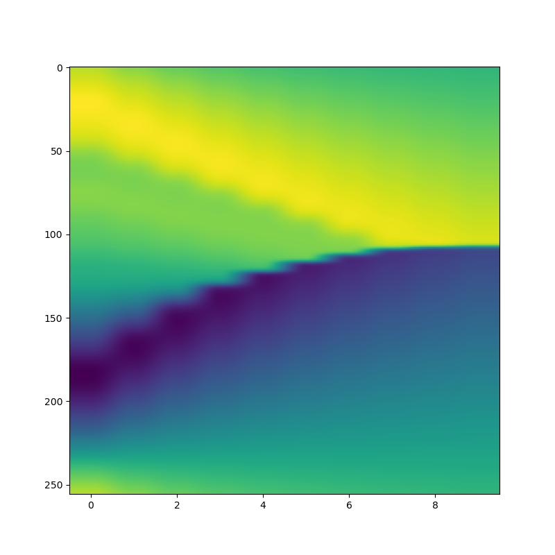
Figure 1. Example of ground truth data for Burgers’ dynamics where $\vec{x}$-axis is time and $\vec{y}$-axis represents space

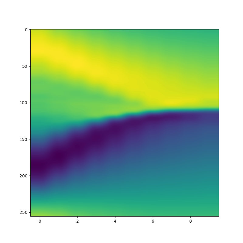
Figure 2. Example of model’s prediction for Burgers’ dynamics where $\vec{x}$-axis is time and $\vec{y}$-axis represents space

References

- [1] Universal approximation to nonlinear operators by neural networks with arbitrary activation functions and its application to dynamical systemsChenTianpingChenHongIEEE transactions on neural networks64911–9171995IEEE@article{chen, title = {Universal approximation to nonlinear operators by neural networks with arbitrary activation functions and its application to dynamical systems}, author = {Chen, Tianping}, author = {Chen, Hong}, journal = {IEEE transactions on neural networks}, volume = {6}, number = {4}, pages = {911–917}, year = {1995}, publisher = {IEEE}}
- [3] Neural ordinary differential equationsChenRicky TQRubanovaYuliaBettencourtJesseDuvenaudDavid KAdvances in neural information processing systems312018@article{NODE, title = {Neural ordinary differential equations}, author = {Chen, Ricky TQ}, author = {Rubanova, Yulia}, author = {Bettencourt, Jesse}, author = {Duvenaud, David K}, journal = {Advances in neural information processing systems}, volume = {31}, year = {2018}}
- [5] Computational galerkin methodsFletcherClive AJ1984Springer@book{Fle, title = {Computational galerkin methods}, author = {Fletcher, Clive AJ}, year = {1984}, publisher = {Springer}}
- [7] On the approximate realization of continuous mappings by neural networksFunahashiKen-IchiNeural networks23183–1921989Elsevier@article{Fun, title = {On the approximate realization of continuous mappings by neural networks}, author = {Funahashi, Ken-Ichi}, journal = {Neural networks}, volume = {2}, number = {3}, pages = {183–192}, year = {1989}, publisher = {Elsevier}}
- [9] Multilayer feedforward networks are universal approximatorsHornikKurtStinchcombeMaxwellWhiteHalbertNeural networks25359–3661989Elsevier@article{Horn, title = {Multilayer feedforward networks are universal approximators}, author = {Hornik, Kurt}, author = {Stinchcombe, Maxwell}, author = {White, Halbert}, journal = {Neural networks}, volume = {2}, number = {5}, pages = {359–366}, year = {1989}, publisher = {Elsevier}}
- [11] Topological methods in the theory of nonlinear integral equationsKrasnosel’skiiYu PPergamon Press1964@article{Topological, title = {Topological methods in the theory of nonlinear integral equations}, author = {Krasnosel'skii, Yu P}, journal = {Pergamon Press}, year = {1964}}
- [13] Multilayer feedforward networks with a nonpolynomial activation function can approximate any functionLeshnoMosheLin, Vladimir YaPinkusAllanSchocken, ShimonNeural networks66861–8671993Elsevier@article{LLPS, title = {Multilayer feedforward networks with a nonpolynomial activation function can approximate any function}, author = {Leshno, Moshe}, authro = {Lin, Vladimir Ya}, author = {Pinkus, Allan}, auhtor = {Schocken, Shimon}, journal = {Neural networks}, volume = {6}, number = {6}, pages = {861–867}, year = {1993}, publisher = {Elsevier}}
- [15] Fourier neural operator for parametric partial differential equationsLiZongyiKovachkiNikolaAzizzadenesheliKamyarLiuBurigedeBhattacharyaKaushikStuartAndrewAnandkumarAnimaInternational Conference on Learning Represetnations2021@article{FNO, title = {Fourier neural operator for parametric partial differential equations}, author = {Li, Zongyi}, author = {Kovachki, Nikola}, author = {Azizzadenesheli, Kamyar}, author = {Liu, Burigede}, author = {Bhattacharya, Kaushik}, author = {Stuart, Andrew}, author = {Anandkumar, Anima}, journal = {International Conference on Learning Represetnations}, year = {2021}}
- [17] Learning nonlinear operators via deeponet based on the universal approximation theorem of operatorsauthor=Jin, PengzhanLu, LuPangGuofeiZhangZhongqiangKarniadakisGeorge EmNature machine intelligence33218–2292021Nature Publishing Group UK London@article{DeepOnet, title = {Learning nonlinear operators via DeepONet based on the universal approximation theorem of operators}, author = {{Lu, Lu} author={Jin, Pengzhan}}, author = {Pang, Guofei}, author = {Zhang, Zhongqiang}, author = {Karniadakis, George Em}, journal = {Nature machine intelligence}, volume = {3}, number = {3}, pages = {218–229}, year = {2021}, publisher = {Nature Publishing Group UK London}}
- [19] The expressive power of neural networks: a view from the widthLuZhouPuHongmingWangFeichengHuZhiqiangWangLiweiAdvances in neural information processing systems302017@article{Lu, title = {The expressive power of neural networks: A view from the width}, author = {Lu, Zhou}, author = {Pu, Hongming}, author = {Wang, Feicheng}, author = {Hu, Zhiqiang}, author = {Wang, Liwei}, journal = {Advances in neural information processing systems}, volume = {30}, year = {2017}}
- [21] Approximation theory of the mlp model in neural networksPinkusAllanActa numerica8143–1951999Cambridge University Press@article{Pink, title = {Approximation theory of the MLP model in neural networks}, author = {Pinkus, Allan}, journal = {Acta numerica}, volume = {8}, pages = {143–195}, year = {1999}, publisher = {Cambridge University Press}}
- [23] Learning integral operators via neural integral equationsZappalaEmanueleFonsecaAntonio Henrique de OliveiraCaroJosue OrtegaMoberlyAndrew HenryHigleyMichael JamesCardinJessicaDijkDavid vanNature Machine Intelligence1–172024Nature Publishing Group UK London@article{ANIE, title = {Learning integral operators via neural integral equations}, author = {Zappala, Emanuele}, author = {Fonseca, Antonio Henrique de Oliveira}, author = {Caro, Josue Ortega}, author = {Moberly, Andrew Henry}, author = {Higley, Michael James}, author = {Cardin, Jessica}, author = {Dijk, David van}, journal = {Nature Machine Intelligence}, pages = {1–17}, year = {2024}, publisher = {Nature Publishing Group UK London}}
- [25] Neural integro-differential equationsZappalaEmanueleFonsecaAntonio H de OMoberlyAndrew HHigleyMichael JAbdallahChadiCardinJessica Avan DijkDavidProceedings of the AAAI Conference on Artificial Intelligence37911104–111122023@inproceedings{NIDE, title = {Neural integro-differential equations}, author = {Zappala, Emanuele}, author = {Fonseca, Antonio H de O}, author = {Moberly, Andrew H}, author = {Higley, Michael J}, author = {Abdallah, Chadi}, author = {Cardin, Jessica A}, author = {van Dijk, David}, booktitle = {Proceedings of the AAAI Conference on Artificial Intelligence}, volume = {37}, number = {9}, pages = {11104–11112}, year = {2023}}
- [27] Spectral methods for neural integral equationsZappalaEmanuelearXiv preprint arXiv:2312.056542023@article{Spectral, title = {Spectral methods for Neural Integral Equations}, author = {Zappala, Emanuele}, journal = {arXiv preprint arXiv:2312.05654}, year = {2023}}
- [29] Projection methods for operator learning and universal approximationZappalaEmanuelearXiv preprint arXiv:2406.122642024@article{EZ_proj, title = {Projection Methods for Operator Learning and Universal Approximation}, author = {Zappala, Emanuele}, journal = {arXiv preprint arXiv:2406.12264}, year = {2024}}