Mimicking Human Intuition: Cognitive Belief-Driven Q-Learning

Abstract

Reinforcement learning encounters challenges in various environments related to robustness and explainability. Traditional Q-learning algorithms cannot effectively make decisions and utilize the historical learning experience. To overcome these limitations, we propose Cognitive Belief-Driven Q-Learning (CBDQ), which integrates subjective belief modeling into the Q-learning framework, enhancing decision-making accuracy by endowing agents with human-like learning and reasoning capabilities. Drawing inspiration from cognitive science, our method maintains a subjective belief distribution over the expectation of actions, leveraging a cluster-based subjective belief model that enables agents to reason about the potential probability associated with each decision. CBDQ effectively mitigates overestimated phenomena and optimizes decision-making policies by integrating historical experiences with current contextual information, mimicking the dynamics of human decision-making. We evaluate the proposed method on discrete control benchmark tasks in various complicate environments. The results demonstrate that CBDQ exhibits stronger adaptability, robustness, and human-like characteristics in handling these environments, outperforming other baselines. We hope this work will give researchers a fresh perspective on understanding and explaining Q-learning.

1 Introduction

Reinforcement learning (RL) algorithms aim to learn optimally rewarding behaviors by modeling how an agent acquires optimal strategies through a trial-and-error process within an environment (Sutton & Barto, 2018; Sutton et al., 1999). Although RL has achieved significant success in areas like gaming, autonomous driving, and robotics, current algorithms continue to encounter challenges in addressing decision-making issues within complex, dynamic, and uncertain environments (Wu et al., 2024; McAleer et al., 2024; Xu et al., 2020; Watkins & Dayan, 1992; Silver et al., 2016; Mnih et al., 2015; Mao et al., 2020; Zhang et al., 2024; Mao et al., 2022; Guss et al., 2021).

Q-learning, a cornerstone of model-free reinforcement learning (Watkins & Dayan, 1992; Watkins, 1989; Barto et al., 1989), along with its variants like Double Q Learning, has sought to improve learning by minimizing the mean squared Bellman error (MSBE). However, these methods often encounter challenges such as pessimistic value estimates and theoretical limitations (Ren et al., 2021; Hasselt, 2010; Hui et al., 2024), and they frequently fail to address the fundamental reliance on maximal value estimates (Fujimoto et al., 2018).

To overcome these limits, we propose to use a novel approach: Cognitive Science, often seen as a manifestation of human intuition. In this domain, humans typically construct and adjust mental models’ subjective beliefs when confronted with uncertainty to predict future events and make corresponding decisions (Peterson & Beach, 1967; Hastie & Dawes, 2009; Gigerenzer et al., 1991). These mental models, grounded in the cognition and experience of the world, empower humans to assess the potential consequences of various actions and make effective choices in complex settings. Notably, effectively managing uncertainty during decision-making is essential, as it directly influences both the efficiency of learning and the robustness of decisions (Kochenderfer, 2015). By leveraging this mechanism, we apply similar mental model theories to RL to improve the performance and adaptability of algorithms in various environments.

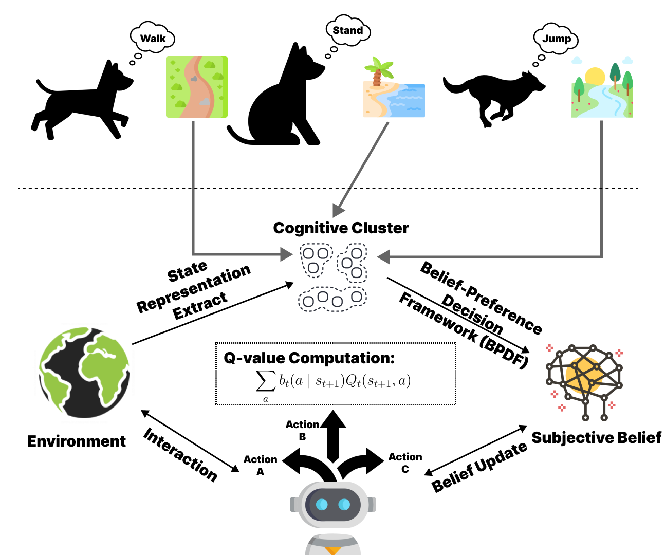
Figure 1: Cognitive Belief-Driven Q-Learning Framework: includes subjective belief components, human cognitive clusters, and BPDF. We provide a vivid example showing how pets make action decisions (e.g., walking, standing, jumping) in response to different environmental states (such as forest paths, oceans, and brooks).

We present a novel direction for enhancing uncertainty optimization in deep Q-learning by integrating cognitive science’s mental model with expected utility theory (Mongin, 1998). We propose Cognitive Belief-Driven Q-Learning (CBDQ), shown in Figure 1, an off-policy deep Q-Learning algorithm applicable to both discrete and continuous states. Specifically, CBDQ incorporates:

(1) Subjective Belief Component (Soltani & Izquierdo, 2019) addresses the overestimation problem in Q-learning. It is grounded in Subjective Expected Utility Theory (Mongin, 1998), a fundamental component of decision theory that evaluates decision options by multiplying the utilities of actions by their associated probabilities. By modeling subjective beliefs, agents simulate how individuals adjust expectations, enhancing learning through probabilistic reasoning.

(2) Human Cognitive Clusters, implemented using the K-means algorithm (Ikotun et al., 2022), emulate how humans categorize information by grouping similar states within the environment’s state space. This method mirrors human cognition, where stimuli or situations are naturally classified into distinct categories, and serve as an efficient tool for state representation extraction. The model compresses high-dimensional data by clustering the state space into meaningful, low-dimensional representations, capturing essential environmental features and reducing learning complexity.

(3) Belief-Preference Decision Framework (BPDF) integrates subjective beliefs and cognitive clusters into a unified decision-making process. BPDF adapts to various state spaces, allowing agents to base decisions on expected outcomes, past experiences (via Human Cognitive Clusters), and current beliefs. This enables context-sensitive decision-making, closely mirroring human cognition in complex, uncertain environments.

Empirical evaluations show that CBDQ consistently achieves higher feasible rewards in different environments, outperforming other advanced Q-learning baselines. This work moves us closer to human-like agents, offering innovative thinking for complex decision-making systems.

2 Related Works

The development of RL can be broadly categorized into two main directions: mathematical optimization and learning process simulation. Both approaches stem from the concept of learning from delayed rewards, originally proposed by (Watkins, 1989).

2.1 Advancements mathematical optimization in Q-Learning

Despite efforts to address overestimation bias, Double Q-Learning (Hasselt, 2010) only partially reduces maximization bias and may still cause underestimation in noisy environments, potentially leading to convergence to near-optimal rather than optimal solutions (Weng et al., 2020; Ren et al., 2021; Wang et al., 2021) proposed ensemble Q-learning as an alternative, using multiple Q-function approximators and conservatively selecting the minimum value. However, this strategy also risks underestimation and performance variability due to approximation errors and the limitations of a fixed ensemble size. In recent years, researchers have developed innovative Q-learning algorithms. For example, (Bas-Serrano et al., 2021) introduced Logistic Q-Learning, using a homoscedastic logistic noise model to reframe value learning via linear programming. (Garg et al., 2023) proposed Extreme Q-Learning (XQL), which utilizes a Gumbel noise source along with the LINEX loss function to more effectively capture the asymmetry in Q-value distributions. (Hui et al., 2023) developed Double Gumbel Q-Learning (DoubleGum), incorporating two heteroscedastic Gumbel noise sources and an adjustable pessimism factor to mitigate estimation bias. These approaches offer crucial theoretical and practical advancements for resolving Q-learning biases. While these optimization-based methods have partially addressed estimation bias, they remain incremental improvements within the Q-learning framework. Logistic Q-Learning has limited use in complex environments, XQL struggles with diverse uncertainties, and though DoubleGum offers a broader theoretical framework, it still faces key challenges, notably the lack of proven convergence. One might question: Is there a unique way of thinking that can improve algorithms like Q-learning?

2.2 Learning Process Insight Algorithms in Reinforcement Learning

Ongoing development in human-like science and RL have increasingly focused on integrating human-like reasoning and beliefs, key components of learning process-oriented algorithms. These models aim to emulate human decision-making by adapting beliefs and strategies based on experience. Complementing these efforts, Barber(Barber, 2012) discusses Bayesian reasoning frameworks that incorporate prior knowledge to manage uncertainty effectively. Building on this, Carroll(Carroll et al., 2019) explored collaboration by integrating learned human policies into Q-learning. More recently, Zhang(Zhang et al., 2021) introduced Solipsistic Reinforcement Learning, extracting human-perspective state representations, while Hu(Hu et al., 2021) developed Off-Belief Learning (OBL), allowing agents to reason about others’ actions with dynamic beliefs. Additionally, O’Donoghue(O’Donoghue, 2021) proposed Variational Bayesian Reinforcement Learning, which offers a novel approach to balancing exploration and exploitation using a risk-seeking utility function. This method introduces a new Bellman operator with associated fixed points, termed ’knowledge values,’ which compress both expected future rewards and epistemic uncertainty into a single value. These approaches enhance AI adaptability and align reinforcement learning with human cognition.

3 Problem Formulation

Markov Decision Processes (MDP) To solve a RL problem, the agent optimizes the control policy under an MDP $\mathcal{M}$, which can be defined by a tuple $(\mathcal{S},\mathcal{A},p_{\mathcal{T}},r,\mu_{0},\gamma,T)$ where: 1) $\mathcal{S}$ and $\mathcal{A}$ denote the space of states and actions. 2) $p_{\mathcal{T}}(s_{t+1}|s_{t},a_{t})$ and $r(s_{t},a_{t})$ define the transition probability and reward function. 3) $\mu_{0}$ defines the initial state distribution. 4) $\gamma\in(0,1)$ is the discount factor and $T$ defines the planning horizon. The goal of the RL policy $\pi(a|s)$ is to maximize expected discounted rewards:

$$\arg\max_{\pi}\mathbb{E}_{\pi,p_{\mathcal{T}},\mu_{0}}\Big{[}\sum_{t=0}^{T}\gamma^{t}r(s_{t},a_{t})\Big{]}$$ (1)

We define the action value function given a policy $\pi$:

$$Q(s,a)=\mathbb{E}_{\pi,p_{\mathcal{T}},\mu_{0}}\big{[}\sum_{t=0}^{T}\gamma^{t}r(s_{t},a_{t})\mid s_{0}=s,a_{0}=a\big{]}$$ (2)

and the optimal Q function is:

$$Q^{*}(s_{t},a_{t})=\mathbb{E}_{\pi,p_{\mathcal{T}},\mu_{0}}\left[r(s_{t},a_{t})+\gamma Q^{*}(s_{t+1},a)\right]$$ (3)

One of our goals is that $Q$ is guaranteed to converge to $Q^{*}(s,a)$ as $t\to\infty$:

$$\lim_{t\to\infty}Q(s_{t},a_{t})=Q^{*}(s_{t},a_{t})$$ (4)

Overestimation Error Letting $Q(s_{t},a_{t};\phi_{i})$ be the action-value function of Q-learning (Watkins & Dayan, 1992) at iteration i, we follow terminology from (Anschel et al., 2016). We denote $\hat{y}_{s,a}^{i}$ is the Q-learning target estimation, and $y_{s,a}^{i}$ is the true target:

$$\hat{y}_{s,a}^{i}=\mathbb{E}_{\mathcal{B}}\left[r(s_{t},a_{t})+\gamma\max_{a}Q(s_{t+1},a;\phi_{i-1})|s_{t},a_{t}\right],$$ (5)

$$y_{s,a}^{i}=\mathbb{E}_{\mathcal{B}}\left[r(s_{t},a_{t})+\gamma\max_{a}(y_{s_{t+1},a}^{i-1})|s_{t},a_{t}\right].$$ (6)

where $\mathcal{B}$ is a replay buffer. We denote $Z_{s_{t},a_{t}}^{i}$ the target approximation error (TAE), and $R_{s_{t},a_{t}}^{i,err}$ is the overestimation error, namely

$$Z_{s_{t},a_{t}}^{i}=Q(s_{t},a_{t};\phi_{i})-\hat{y}_{s_{t},a_{t}}^{i}$$ (7)

$$R_{s_{t},a_{t}}^{i,err}=\hat{y}_{s_{t},a_{t}}^{i}-y_{s_{t},a_{t}}^{i}$$ (8)

(Thrun & Schwartz, 2014) considered the TAE $Z_{s_{t},a_{t}}^{i}$ as a random variable uniformly distributed in the interval $[-\epsilon,\epsilon].$ Due to the max operator in the target estimation $\hat{y}_{s_{t},a_{t}}^{i}$, the expected overestimation errors $\mathbb{E}_{z}[R_{s_{t},a_{t}}^{i,err}]$ are upper bounded by $\gamma\epsilon\frac{k-1}{k+1}$. $K$ is the number of actions. We attempt to overcome this overestimation issue with a unique approach and enhance the capabilities of Q-learning methods.

4 Modelling Subjective Belief Distribution In Q-learning Framework

In this work, we address a fundamental question: How does integrating subjective beliefs refine decision-making within a Q-learning framework? We propose a novel method, Cognitive Belief-Driven Q-Learning (CBDQ) to incorporate human-like subjective belief components into RL. By leveraging Subjective Expected Utility Theory (SEUT), we dynamically update an agent’s belief distribution over time, reflecting evolving perceptions of rewards, actions, and states.

4.1 Expected Utility Theory and Q-learning: A Cognitive Perspective

To closely mirror human cognitive processes, we consider integrating SEUT into RL. SEUT offers a structured framework for decision-making under uncertainty by individual’s belief preference, promoting actions that maximize the weighted sum of outcome utilities. This framework aligns seamlessly with MDPs, where the value function represents a specific form of expected utility derived from discounted returns.

Proposition 4.1

Consider a decision-making scenario in a MDP, where the complete set of possible outcomes is represented by $\mathcal{X}$. Let $b_{t}(\cdot\mid s_{t+1})$ represent the agent’s belief distribution over possible actions in the next state $s_{t+1}$, and $u_{t}(s,x)$ be the utility of outcome $x$ in state $s$. Then the expected utility $U_{t}(s,x)$ at time $t$ is given by:

$$U_{t}(s,x)=\sum_{x\in\mathcal{X}}b_{t}(\cdot\mid s_{t+1})\cdot u_{t}(s,x)$$ (9)

Proposition 4.1 elucidates how individuals evaluate the utility of various actions within a MDP. It not only reflects the core tenets of SEUT but also provides a foundation for understanding learning processes. SEUT simulates how decision-makers assess potential outcomes through a weighted sum of utilities, which directly corresponds to the term $b_{t}(\cdot\mid s_{t+1})\cdot u_{t}(s,x)$ in our formulation. The subjective belief component $b_{t}(\cdot\mid s_{t+1})$ represents an individual’s belief, providing flexibility and robustness for modeling beliefs under uncertainty, aligning our model more closely with human cognitive processes. This characteristic aligns with the closely related cognitive processes proposed by (Tversky & Kahneman, 1992). Concurrently, research by (Hogarth & Einhorn, 1992) demonstrates that individuals revise their beliefs based on new information and experience.

4.2 Evolving Beliefs in Q-Learning

As outlined in proposition 4.1, the expected utility $U_{t}(s,a)$ in a MDP is computed from transition probabilities, rewards, etc. The CBDQ algorithm extends this by replacing the maximum Q-value update with a belief-weighted average of Q-values. We confirm that our Q function can converge to the $Q^{*}$.

Theorem 4.1

Given a finite MDP, the Cognitive Belief-Driven Q-Learning (CBDQ) algorithm, as given by the update rule:

$$Q_{t+1}(s_{t},a_{t})=Q_{t}(s_{t},a_{t})+\alpha_{t}(s_{t},a_{t})\left[r(s_{t},a_{t})+\gamma\sum_{a}b_{t}(a\mid s_{t+1})Q_{t}(s_{t+1},a)-Q_{t}(s_{t},a_{t})\right]$$ (10)

converges with probability 1 to the optimal Q-function, as long as:

$$\sum_{t}\alpha_{t}(s_{t},a_{t})=\infty,\quad\sum_{t}\alpha_{t}^{2}(s_{t},a_{t})<\infty\quad\text{for all}\ (s_{t},a_{t})\in\mathcal{S}\times\mathcal{A}.$$ (11)

To establish Theorem 4.1, we need an auxiliary result from stochastic approximation. You can check the convergence proof section in Appendix D.

It is important to note that while our method bears formal similarities to Expected SARSA, the introduced belief distribution $b_{t}(a\mid s_{t+1})$ fundamentally differs from the agent’s actual action policy. $b_{t}(a\mid s_{t+1})$ represents the agent’s subjective estimation of future states and rewards, influencing Q-value updates without directly determining action selection. The exploration policy (e.g., $\epsilon$-greedy) is responsible for action selection, ensuring comprehensive exploration of all state-action pairs. For algorithm convergence, $b_{t}(a\mid s_{t+1})$ must converge over time to selecting the action with the maximum Q-value, while the exploration policy maintains randomness to ensure non-zero probability of visiting all states. A parametric form for $b_{t}(a\mid s_{t+1})$ can be updated based on state transitions and rewards, similar to the probability smoothed Q-learning approach. (See Appendix A for more on the differences between Expected SARSA and CBDQ.)

Now we will demonstrate how CBDQ addresses the overestimation issue and introduce a lemma to assist us in solving this problem.

Lemma 4.1

Consider a MDP with state $s_{t+1}$ and actions $a$, along with Q-value estimates $\tilde{Q}_{t}(s_{t+1},a)$, where $\tilde{Q}_{t}(s_{t+1},a)$ is assumed to be unbiased for each $a$. Let $b_{t}(a\mid s_{t+1})$ denote the probability of selecting action $a$ in state $s_{t+1}$. By Jensen’s inequality, for any convex function $f$ and random variable $X$, $\mathbb{E}[f(X)]\geq f(\mathbb{E}[X])$. Applying this to our setting yields:

$$\sum_{a}b_{t}(a\mid s_{t+1})\tilde{Q}_{t}(s_{t+1},a)\leq\max_{a}\tilde{Q}_{t}(s_{t+1},a)$$ (12)

Lemma 4.1 establishes the theoretical basis for using subjective belief probability distributions in Q-value updates. By incorporating a belief distribution, the target value $\sum_{a}b_{t}(a\mid s_{t+1})Q_{t}(s_{t+1},a)$ acts as a ”downward estimate” of the maximum Q-value, reducing overestimation and improving the stability and reliability of Q-value updates.

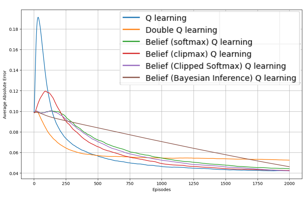
(a) Convergence of Belief Q-Learning vs Standard and Double Q-Learning

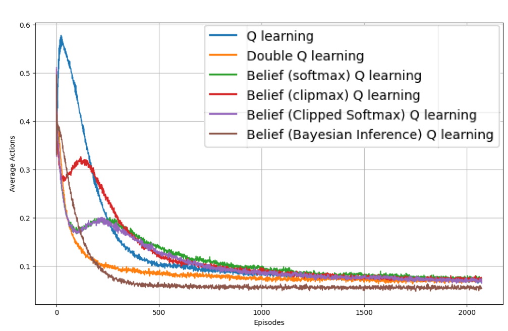
(b) Maximization Bias in Q-learning: Action Selection from Suboptimal States

Figure 2: Two key aspects of maximization bias in Q-learning and its variants. (a) compares the convergence of $|\tilde{Q}-Q^{*}|$ across belief Q-learning, standard Q-learning, and Double Q-learning. Belief Q-learning significantly reduces overestimation of Q-values while converging faster than Double Q-learning. (b) shows the fraction of times the suboptimal ”Left” action is chosen from state A, demonstrating the effect of maximization bias in standard Q-learning.

We conducted experiments based on Example 6.7 in (Sutton & Barto, 2018)’s research (MBP) to verify the effectiveness of dynamically updating the subjective belief model. Four smoothing strategies, each employing a different fixed subjective belief probability model (Softmax, Clipped Max, Clipped Softmax, and Bayesian Inference), detail in Appendix C are compared with Q-learning and Double Q-learning to demonstrate the universality and accuracy of the dynamic updating mechanism for managing uncertainty.

Figure 2 highlights differences in convergence speed and estimation bias across algorithms, with Belief Q-learning using Bayesian inference showing superior stability and convergence to the optimal value, underscoring the importance of dynamic belief updating and prior knowledge in decision-making (Barber, 2012).

Our studies suggest that relying solely on Q-values for probability models lacks robustness in diverse environments. Even Bayesian inference, while incorporating prior knowledge, is constrained by fixed distribution models. In contrast, human decision-making dynamically adjusts subjective belief probabilities based on accumulated experience, enabling better adaptation to complex and changing environments.

4.3 Belief Interaction and Update

Because of the limitations of fixed belief frameworks, we explore the application of dynamic beliefs from the perspective of learning processes. Figure 1 illustrates animals’ subjective belief-based decision-making process in various contexts. This process reflects how agents simplify decision-making through state-space clustering, utilizing a strategy that groups states based on shared features (Liu et al., 2024).

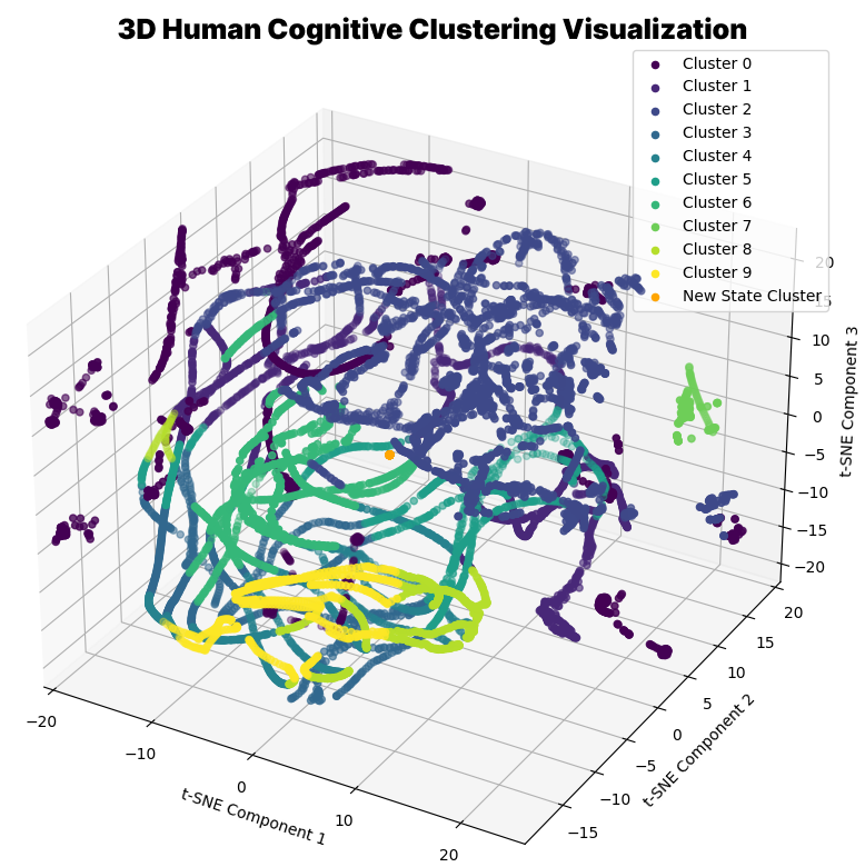
Figure 3: Cognitive Cluster Visualization for LunarLander. We utilized the t-SNE algorithm to map the high-dimensional state features into 3 dimensions. The orange points represent newly received states. If the closest cluster to them is Cluster 2, they will be automatically classified into Cluster 2.

To model belief interaction and update, we introduce Belief-Preference Decision Framework (BPDF), which offers a structured approach to decision-making by integrating human prior knowledge with immediate belief updates. This framework enhances the efficiency and interpretability of decisions in complex environments. The model utilizes human expert knowledge to identify and select informative state features for representation learning. Additionally, clustering algorithms are applied to partition the state space $\mathcal{S}$ into $N$ semantically meaningful and internally consistent clusters $\{\mathcal{C}_{n}\}_{n=1}^{N}$, Figure 3 presents an example within the Box2D environment, adhering to the following formal criteria:

$$\mathcal{S}=\bigcup_{n=1}^{N}\mathcal{C}_{n},\quad\mathcal{C}_{i}\cap\mathcal{C}_{j}=\emptyset,\forall i\neq j$$ (13)

Human cognition and belief formation are gradual processes, where early decisions rely on immediate rewards. Cognitive science research suggests that in uncertain environments, humans initially depend on short-term feedback, progressively incorporating long-term preferences as experience accumulates (Doya, 2007; Gershman et al., 2015). This shift from reward-driven choices to informed decisions underpins the dynamic belief framework we propose. The clusters in our model balance real-time beliefs with prior preferences, mirroring human cognition. This process ensures that, as the agent refines its beliefs, action selection converges to the optimal one, guaranteeing maximum utility. To balance immediate beliefs and prior preferences, the BPDF model updates subjective belief distribution $b_{t}(a\mid s_{t+1})$:

$$b_{t}(a\mid s_{t+1})=(1-\beta_{t})\cdot\hat{b}_{t}(a|s_{t+1})+\beta_{t}\cdot p_{k}(a|s_{t+1})$$ (14)

where $\beta_{t}\in[0,1]$ is a time-varying weight parameter that balances the influence between $\hat{b}_{t}(a\mid s_{t+1})$, representing the smoothed immediate reward strategy, and $p_{k}(a\mid s_{t+1})$, which reflects the subjective belief distribution for action selection in state $s_{t+1}$. After executing each action $a_{t}$, the BPDF model records the state-action pair in the corresponding cluster $\mathcal{C}_{k}$ and updates $p_{k}(a|s_{t+1})$ accordingly. This iterative process allows the model to continuously refine its decision-making strategy by integrating newly acquired knowledge while leveraging prior beliefs. The BPDF records action choices within each state cluster $\mathcal{C}_{k}$, computing the action selection probability distribution $p_{k}(a|s_{t+1})$:

$$p_{k}(a|s_{t+1})=\frac{f(a\mid s\in\mathcal{C}_{k})}{\sum_{\tilde{a}\in\mathcal{A}}f(\tilde{a}\mid s\in\mathcal{C}_{k})}$$ (15)

The clustering approach in our model, inspired by natural categorization mechanisms observed in human and animal cognition, plays a crucial role in extracting meaningful representations from complex state spaces (Botvinick et al., 2020; Rudin, 2019). This process, known as conceptualization or categorization in cognitive science, enables efficient deciding intricate environments by classifying similar states based on experience (Rosch & Mervis, 1975; Markman & Ross, 2003). Unlike models with fixed probability spaces, the dynamic belief updating mechanism optimizes decision-making by continuously adapting to changes, effectively compressing high-dimensional state spaces into manageable representations.

Algorithm 1 Cognitive Belief-Driven Q-Learning Algorithm

1:Q function $Q(s,a;\phi)$, target Q function$Q(s,a;\phi^{-})$, learning rate $\alpha$, discount factor $\gamma$, running steps $T$, episodes $E$, replay buffer $\mathcal{B}$ and exploration probability $\epsilon$

2:$Q^{CBDQ}(s,a;\phi_{T})$

3:Initialize $Q(s,a;\phi)$ with random weights $\phi_{0}$;

4:Initialize replay buffer $\mathcal{B}$ with a fixed length;

5:Initialize Belief-Preference Decision Framework (BPDF) $\{\mathcal{C}_{n}\}^{N}_{n=1}$;

6:Initialize a $\epsilon$-greedy exploration procedure: Explore($\cdot$)

7:for $i=0$ ; $i<E$ ; $i++$ do

8:     Get initial state $s_{0}$ from the environment

9:     for $t=0$ ; $t<T$ ; $t++$ do

10:         Choose action $a_{t}$ using $\epsilon$-greedy: $a_{t}\sim\mathcal{U}(0,1)$

11:         Execute $a_{t}$ to get reward $r(s_{t},a_{t})$, next state $s_{t+1}$

12:         Store $(s_{t},a_{t},r(s_{t},a_{t}),s_{t+1})$ into $\mathcal{B}$

13:         Find the cognitive cluster ${\mathcal{C}_{i}}$ of $s_{t}$, update the count of $a_{t}$ in ${\mathcal{C}_{i}}$

14:         Sample $N$ tuples from $\mathcal{B}$ to update $Q$ function:

15:           $y^{i}_{s_{t},a_{t}}=\mathbb{E}_{\mathcal{B}}\left[r(s_{t},a_{t})+\gamma\sum_{a}b_{t}(a\mid s_{t+1})Q(s_{t+1},a;\phi^{-})|s_{t},a_{t}\right]$

16:           The computation of $b_{t}(a\mid s_{t+1})$ in Equation 14 dynamically integrates immediate rewards and subjective beliefs, enabling continuous adaptation based on evolving information.

17:           $Loss=\mathbb{E}_{\mathcal{B}}\left[(y_{s_{t},a_{t}}^{i}-Q(s_{t},a_{t};\phi))^{2}\right]$

18:         Update $\phi^{-}$;

19:     end for

20:end for

5 Experiment

Running Setting.

For a comprehensive comparison, we employ Feasible Cumulative Rewards metric, which calculates the total rewards accumulated by the agent across all environments (higher is better). We run experiments with three different seeds (123, 321, and 666) and present the mean ± std results for each algorithm. To ensure a fair comparison, we maintain the same settings and parameters for all baselines. Our code is implemented based on the XuanCe benchmark (Liu et al., 2023). Appendix E.4 reports the detailed parameters.

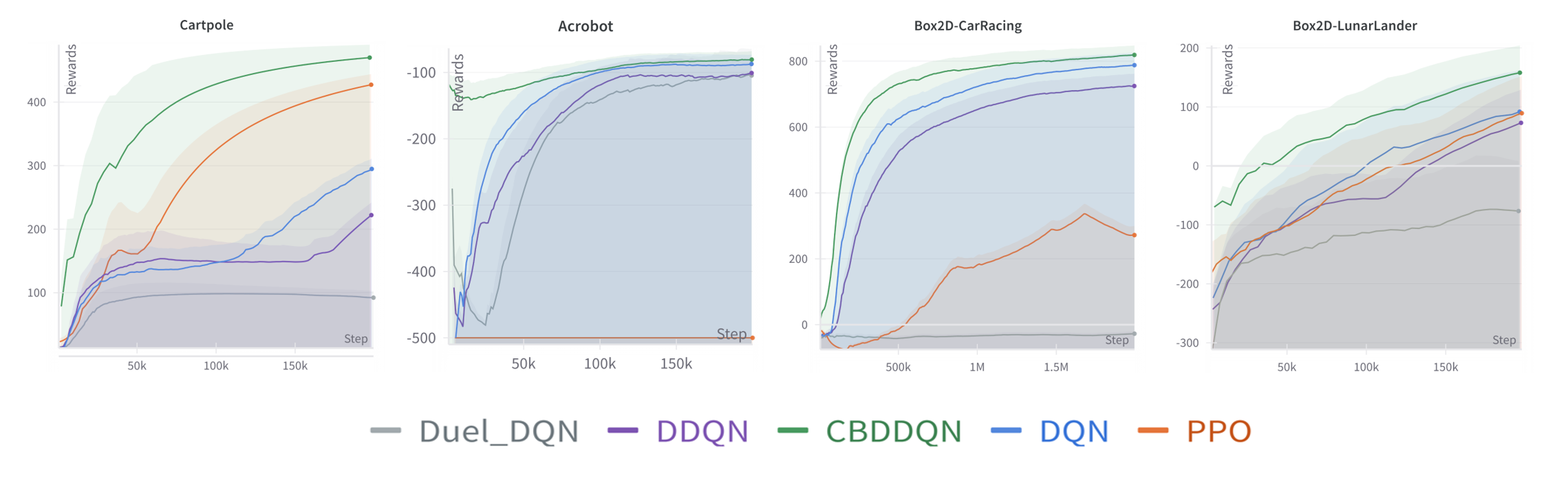
Figure 4: Feasible cumulative rewards. From left to right, the environments are Cartpole, CarRacing and LunarLander.

Comparison Methods.

We consider CBDQ (Algorithm 1) alongside the following baselines: (1) DQN (Mnih et al., 2013) approximates the action-value function using a deep neural network, with experience replay and target networks for stabilization. (2) DDQN improves on this by separating action selection from value estimation, reducing overestimation bias. (3) DuelDQN further enhances learning efficiency through a dual-stream architecture that individually estimates state values and action advantages. (4) PPO uses a clipped objective function for stable policy updates, balancing exploration and exploitation while maintaining a trust region for policy improvements.

5.1 Empirical Evaluations in Physical Simulation Environments

The environments shown in Figure 4 and Appendix F highlight the performance of various RL algorithms across three distinct Classic Control and Box2D tasks (Towers et al., 2024; Parberry, 2017). The leftmost column displays the Cartpole environment, where agents are tasked with balancing a pole on a moving cart. Next is the Acrobot environment, where the goal is to swing a two-link arm to reach a specific height. The third column showcases the CarRacing task, a more complex scenario where agents must control a car to drive smoothly along a racetrack. Finally, the rightmost column presents the LunarLander environment, where agents must carefully land a spaceship on the moon’s surface. Each environment progressively tests different control and decision-making skills, from balancing and swinging dynamics to managing more complex trajectories and landings.

Figure 4 illustrates CBDQ significantly significant improvements with faster convergence by leveraging subjective belief modeling and cognitive clustering. It outperforms all other approaches, generating stable, high-reward trajectories that closely resemble optimal policies. In contrast, without the BPDF, traditional Q algorithms struggle with slower convergence and lower final rewards. While PPO shows moderate improvements, it still suffers from inefficiencies in these environments.

5.2 Empirical Evaluations in Complex Traffic Scenarios

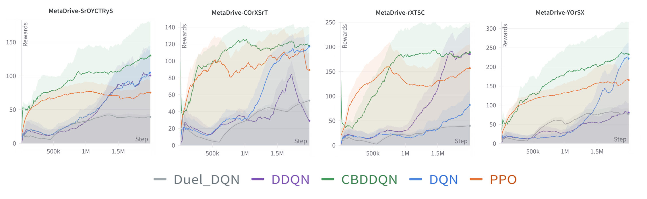
Figure 5: Feasible cumulative rewards. From left to right, the maps are SrOYCTRyS, COrXSrT, rXTSC, and YOrSX.

To evaluate the human-like decision-making and path-planning capabilities of our algorithm, we employ four complex environments within MetaDrive, each designed to mimic real-world driving scenarios that require human-like adaptability (Li et al., 2022). Different letter combinations represent various types of road combinations. More detail of map design is in the Appendix.

Figure 5 and Appendix F present the obvious advantages of CBDQ, particularly in emulating human-like learning and decision-making. Compared to other algorithms, CBDQ demonstrates faster learning, greater stability, and superior final performance. Traditional Q-learning methods like Double DQN, Duel DQN, and DQN show significantly slower convergence and achieve lower rewards, indicating their limitations in handling the complexity of this environment. Unlike PPO, which often converges to suboptimal solutions, CBDQ’s learning curve rises quickly and steadily improves, reflecting its ability to adapt and optimize in complex environments, avoiding local optima. Its strong adaptability to high-dimensional state spaces, dynamic obstacles, and varied road conditions mirrors human decision-making under uncertainty. The superior trajectory smoothness, intersection handling, and road structure adaptability of CBDQ underscore its progress in replicating human-like driving behavior.

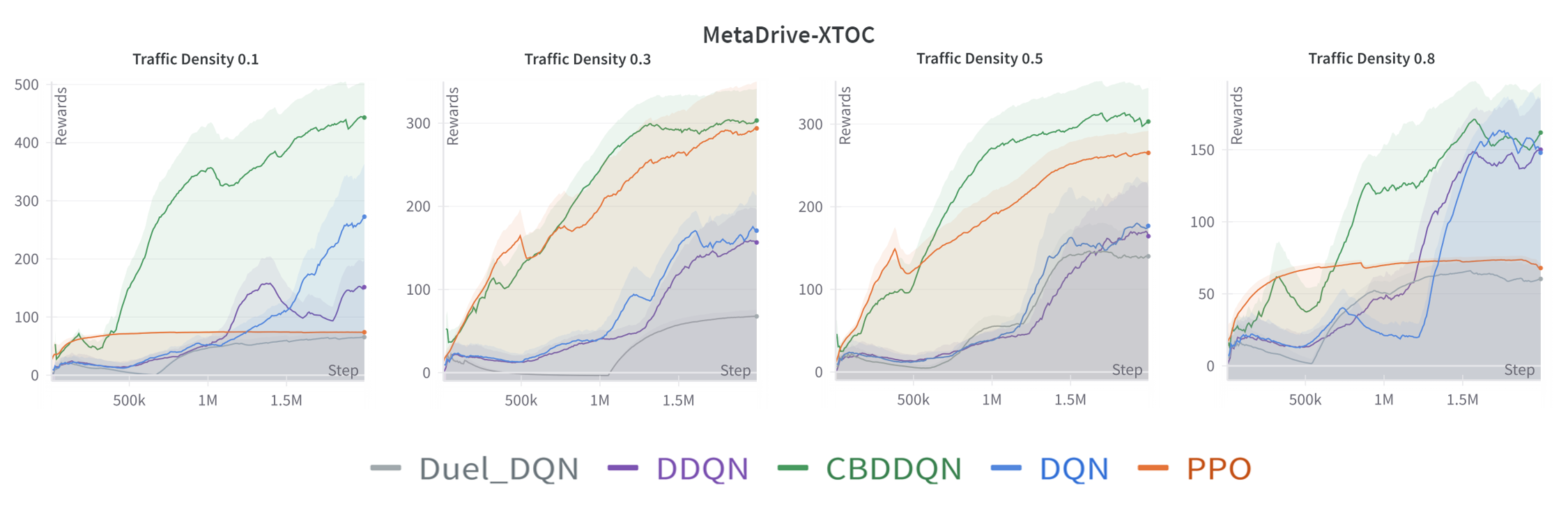
Figure 6: This figure compares the performance of different reinforcement learning algorithms under varying traffic densities (0.1, 0.3, 0.5, and 0.8) in the XTOC Map.

To assess driving control and decision-making at varying levels of difficulty, we conducted experiments with different traffic densities on the XTOC map. As traffic density increased, the system faced progressively complex challenges. Each sub-graph reflects the rewards obtained by agents as they learn to navigate through traffic at increasing levels of density.

Figure 6 and Appendix F highlight the superior performance of CBDQ across varying traffic densities, excelling particularly under high-density conditions. As traffic density increases, decision complexity grows, testing the system’s ability to manage more intricate scenarios. While low-density traffic primarily challenges basic driving functions, high-density conditions require more complex decision-making and adaptive path adjustments. Leveraging the BPDF framework, CBDQ efficiently handles long-term planning, multi-lane interactions, and real-time risk management, consistently achieving higher reward values. PPO and traditional Q methods, though stable at moderate traffic densities, exhibit greater fluctuation in learning and decision-making under low- and high-density traffic, ultimately lagging behind CBDQ in both consistency and rewards.

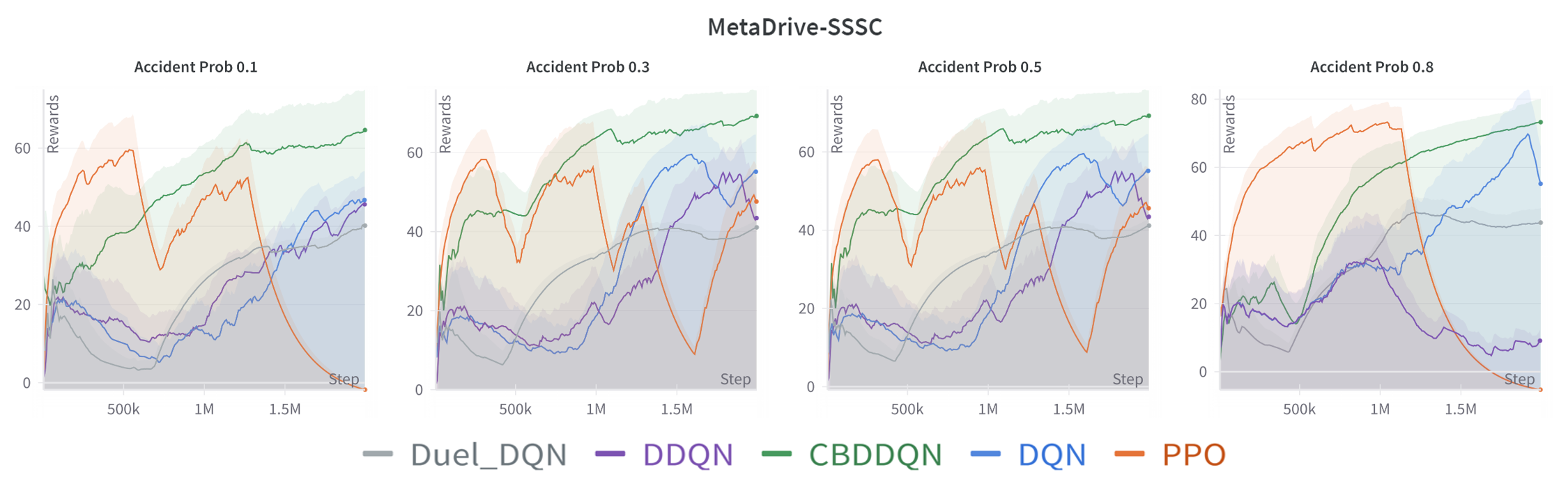
Figure 7: This figure compares the performance of different reinforcement learning algorithms under varying accident probability (0.1, 0.3, 0.5, and 0.8) in the SSSC Map.

In this experiment, we compare the performance of various algorithms under progressively increasing accident probabilities to evaluate their adaptability and decision-making capabilities in high-risk driving scenarios on the SSSC map (See Figure 7 and Appendix F). As the probability of accidents rises from 0.1 to 0.8, the complexity of the driving environment intensifies, requiring the algorithms to navigate regular driving challenges while also responding swiftly to sudden and unexpected risks. This setup tests the algorithms’ ability to manage real-time dynamic environments, focusing on their long-term planning, risk avoidance, and decision stability under escalating uncertainty.

The experimental results indicate that CBDQ consistently outperforms other algorithms across all accident probability levels. At low and moderate accident rates, CBDQ demonstrates robust learning and stability, handling basic driving challenges while adapting efficiently to moderate risk scenarios. However, its advantage becomes more pronounced in high-risk environments, where accident probabilities reach 0.8. In these situations, CBDQ shows superior decision stability and maintains higher reward values compared to algorithms like PPO and DQN, which exhibit greater volatility and struggle to maintain performance as risks escalate. This highlights the strength of CBDQ’s belief-driven decision-making framework in navigating uncertainty and managing sudden hazards in dynamic driving environments.

6 Future Insight

Expanding to Continuous Control Domains.

Building on our success in discrete environments, we are exploring ways to adapt our framework to continuous control scenarios. This involves integrating cognitive science principles with advanced reinforcement learning techniques, aiming for more flexible and robust decision-making in complex, continuous action spaces.

Human-like Learning Processes in Reinforcement Learning.

CBDQ provides new insights for future reinforcement learning, particularly in emulating human learning processes. Future algorithms are expected to increasingly simulate human concept formation and abstract reasoning, with cognitive clustering evolving into autonomously formed conceptual hierarchies. Additionally, dynamic belief updating mechanisms point toward adaptive learning rates and exploration strategies, where algorithms adjust based on task complexity and learning progress. CBDQ’s strengths in uncertainty management and long-term planning suggest that human decision psychology will play a greater role in future reinforcement learning.

7 Conclusion

This study introduces the Cognitive Belief-Driven Q-learning (CBDQ) algorithm, integrating cognitive science principles with reinforcement learning to enhance efficiency and interpretability in complex environments. CBDQ incorporates subjective belief probabilistic reasoning and cognitive clustering for state space representation, demonstrating superior performance over traditional Q-learning and advanced algorithms like PPO. This research has broad implications for AI, potentially catalyzing interdisciplinary innovations toward more intelligent, interpretable, and adaptable systems capable of interesting environments.

Acknowledgments

I would like to express my deepest gratitude to my advisor, Professor David Barber at UCL, and Professor Chris Watkins at Royal Holloway, University of London, for their invaluable guidance and for inspiring this research with their profound insights into human-like learning processes. Both UCL and Royal Holloway have been my alma maters, where I not only grew academically but also experienced some of the most joyful and unforgettable moments of my life.

This research builds upon the foundational work of Professor David Barber. I completed it after my graduation from UCL, and I am immensely grateful for the continuous support provided by the UCL Centre for Artificial Intelligence. My heartfelt thanks go to all those who contributed to this journey, offering their wisdom, time, and encouragement.

Finally, I would like to extend my deepest appreciation to my lover, Ms. Yiner He, whose unwavering support has been instrumental throughout this journey. Her encouragement has been a pillar of strength, allowing me to cherish the unforgettable memories I made during my time at UCL.

Appendix A Comparison of Expected SARSA and CBDQ

Feature	Expected SARSA	Cognitive Belief-Driven Q-learning
Policy Type	On-policy	Off-policy
Action Selection	Single policy $\pi(a|s)$ for both experience generation and updates	Exploration policy for experience, $b_{t}(a|s_{t+1})$ distribution for updates
Convergence Target	True action-value function of the current policy	Optimal Q-value function (under specific conditions)
Exploration-Exploitation	Controlled by single policy $\pi$	Exploration policy and $b_{t}$ distribution can be adjusted independently
Sample Utilization	Only uses samples from current policy	Can utilize samples from any policy
Main Advantage	Directly evaluates current policy, potentially faster convergence	More flexible, potentially more stable, can find optimal policy
Suitable Scenarios	Online learning, need for quick policy evaluation	Offline learning, need to find optimal policy

Table 1: Comparison between Expected SARSA and Smoothed Q-learning

Appendix B MBP Experiment

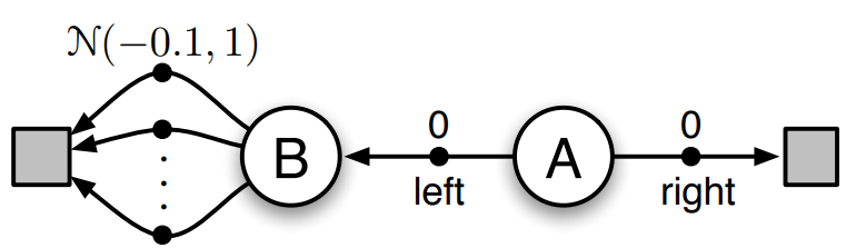
Figure 8: Experimental Setup of the Maximization Bias Problem (MBP): The experiment starts in state A. The agent has two possible actions: Right, leading to terminal state C with zero reward, and Left, which leads to state B, also with zero reward. In state B, the agent has 8 actions, each leading to terminal state D with a reward sampled from a Gaussian distribution with a mean of -0.1 and a variance of 1. This setup illustrates maximization bias in traditional Q-learning algorithms, where overestimation can occur due to variance in the rewards(Sutton & Barto, 2018).

Purpose of the Experiment

This setup underscores the issue of maximization bias in traditional Q-learning, where the algorithm selects actions based on the highest Q-value. In state B, the variability in rewards amplifies this bias, as Q-learning tends to overestimate the expected reward by favoring actions with initially higher but unreliable Q-values. Over time, this can lead the agent to consistently choose suboptimal actions, even when more stable options offer better long-term results.

Appendix C Smoothing Strategy

Strategy	Formula
Softmax	$b_{t}=\frac{e^{Q(s,a)}}{\sum_{b}e^{Q(s,b)}}$
Clipped Max	$$b_{t}=\begin{cases}1-\tau,&\text{if }a=a^{*}\\ \frac{\tau}{A-1},&\text{if }a\neq a^{*}\end{cases}$$
Clipped Softmax	$$b_{t}=\begin{cases}\frac{e^{\beta Q(s,a)}}{\sum_{b\in I}e^{\beta Q(s,b)}},&\text{if }a\in I\\ 0,&\text{if }a\notin I\end{cases}$$
Bayesian Inference	$$Q_{\text{adjusted}}(s,a)=Q(s,a)+\mu_{\text{prior}}$$ $$b_{t}=\frac{e^{Q_{\text{adjusted}}(s^{\prime},a)}}{\sum_{b}e^{Q_{\text{adjusted}}(s^{\prime},b)}}$$ $$\sigma_{\text{posterior}}^{2}=\left(\frac{1}{\sigma_{\text{prior}}^{2}}+\frac{n}{\sigma_{\text{observation}}^{2}}\right)^{-1}$$ $$\mu_{\text{posterior}}=\sigma_{\text{posterior}}^{2}\left(\frac{\mu_{\text{prior}}}{\sigma_{\text{prior}}^{2}}+\sum_{i=1}^{n}\frac{r_{i}}{\sigma_{\text{observation}}^{2}}\right)$$

Table 2: Smoothing strategies with respective formulas

Appendix D Convergence Proof

We outline a proof that builds upon the following result (Singh et al., 2000; Barber, 2023) for a formal statement) and follows the framework provided in (Melo, 2001):

Theorem 1 The random process $\{\Delta_{t}\}$ taking value in $\mathbb{R}$ and defined as

$$\Delta_{t+1}(x)=(1-\alpha_{t}(x))\Delta_{t}(x)+\alpha_{t}(x)F_{t}(x)$$ (16)

converges to 0 with probability 1 under the following assumptions:

• $0\leq\alpha_{t}\leq 1$, $\sum_{t}\alpha_{t}(x)=\infty$, $\sum_{t}\alpha_{t}^{2}(x)<\infty$;

• $\mathbb{E}[\|F_{t}(x)\|_{W}]\leq\kappa\|\Delta_{t}\|_{W}+c_{t}$, $\kappa\in[0,1)$ and $c_{t}\to 0$ with probability 1;

• $\text{var}(F_{t}(x))\leq C(1+\|\Delta_{t}\|_{W})^{2}$, $C>0$

where $\|\Delta_{t}\|_{W}$ denotes a weighted max norm.

We are interested in the convergence of $Q_{t}$ towards the optimal value $Q_{*}$ and therefore define

$$\Delta_{t}=Q_{t}(s_{t},a_{t})-Q_{*}(s_{t},a_{t})$$ (17)

It is convenient to write the smoothed update as

$$Q_{t+1}(s_{t},a_{t})=Q_{t}(s_{t},a_{t})+\alpha_{t}(s_{t},a_{t})\left(r_{t}+\gamma\left\langle Q(s_{t+1},a)\right\rangle_{a}-Q_{t}(s_{t},a_{t})\right)$$ (18)

where $\langle f(x)\rangle_{x}$ means the expectation of the function $f(x)$ with respect to the distribution of $x$. Using the smoothed update, we can write

$$\Delta_{t+1}(s_{t},a_{t})=Q_{t+1}(s_{t},a_{t})-Q_{*}(s_{t},a_{t})$$ (19)

$$=(1-\alpha_{t})\Delta_{t}+\alpha_{t}\left(r_{t}+\gamma\langle Q(s_{t+1},a)\rangle_{a}-Q_{*}(s_{t},a_{t})\right)$$ (20)

In terms of Theorem 1, we therefore define

$$F_{t}=r_{t}+\gamma\sum_{a}b_{t}(a|s_{t+1})Q_{t}(s_{t+1},a)-Q_{*}(s_{t},a_{t})$$ (21)

Proof D.1

For convergence, we need to bound the norm of the expected value of $F_{t}$. We can write

$$\frac{1}{\gamma}\mathbb{E}[F_{t}]=\mathbb{E}_{p_{\mathcal{T}}}[G_{t}]$$ (22)

where

$$G_{t}=\sum_{a}b_{t}(a|s_{t+1})Q_{t}(s_{t+1},a)-\max_{a}Q_{*}(s_{t+1},a)$$ (23)

we can form the bound

$$\frac{1}{\gamma}\mathbb{E}[F_{t}]_{\infty}=\mathbb{E}[\|G_{t}\|_{\infty}]\leq\|G_{t}\|_{\infty}$$ (24)

which means that if we can bound $\|G_{t}\|_{\infty}$ appropriately, the mean criterion will be satisfied.

Assuming that $b_{t}$ places $(1-\delta_{t})$ mass in the maximal state of $Q$, we can write

$$\|G_{t}\|_{\infty}\leq\left\|\max_{a}Q_{t}(s_{t+1},a)-\max_{a}Q_{*}(s_{t+1},a)\right\|_{\infty}+\delta_{t}\left\|\max_{a}Q_{t}(s_{t+1},a)-\sum_{c\neq a}b_{t}(c|s_{t+1})Q_{t}(s_{t+1},c)\right\|_{\infty}$$ (25)

$$\leq\|\Delta_{t}\|_{\infty}+\delta_{t}\left\|\max_{a}Q_{t}(s_{t+1},a)-\sum_{c\neq a}b_{t}(c|s_{t+1})Q_{t}(s_{t+1},c)\right\|_{\infty}$$ (26)

$$\leq\|\Delta_{t}\|_{\infty}+\delta_{t}\left(\|\max_{a}Q_{t}(s_{t+1},a)\|_{\infty}+\|Q_{t}(s_{t+1},c_{-})\|_{\infty}\right)$$ (27)

where $c_{-}=\arg\min_{c\neq a}Q_{t}(s_{t+1},c)$ and the penultimate line follows from the fact that only a maximum of $\delta_{t}$ mass can be placed in the minimal state $c_{-}$ (since $(1-\delta_{t})$ mass is placed in state $a_{*}$). Putting this together we have

$$\mathbb{E}[F_{t}]_{\infty}\leq\gamma\|\Delta_{t}\|_{\infty}+\gamma\delta_{t}\left(\|\max_{a}Q_{t}(s_{t+1},a)\|_{\infty}+\|Q_{t}(s_{t+1},c)\|_{\infty}\right)$$ (28)

Since the $Q_{t}$ are bounded and $\mathbb{E}[F_{t}]$ converges to zero with probability 1, provided $\delta_{t}$ converges to 0 with probability 1. The mean criterion is therefore satisfied.

For the variance criterion, since the rewards are bounded, $Q_{t}$ and $\Delta_{t}$ are also bounded. This means that the variance is bounded. We can write:

$$\Delta F_{t}=\Delta r+\gamma\left\langle\left(Q_{t}(s_{t+1},a)-\langle Q_{t}(s_{t+1},a)\rangle\right)\right\rangle_{s_{t+1},a}$$ (29)

$$=\Delta r+\gamma\left\langle\left(Q_{t}(s_{t+1},a)\right)_{a}-\left(Q_{*}(s_{t+1},a)\right)_{a}+\left(Q_{*}(s_{t+1},a)\right)_{a}-\langle Q_{t}(s_{t+1},a)\rangle_{a}\right\rangle_{s_{t+1}}$$ (30)

$$=\Delta r+\gamma\left\langle Q_{t}(s_{t+1},a)-Q_{*}(s_{t+1},a)-\gamma\left\langle Q_{t}(s_{t+1},a)\right\rangle_{s_{t+1}}\right\rangle_{a}$$ (31)

We can bound the variance using

$$\text{var}(F_{t})=\|\langle\Delta F_{t}\rangle\|_{\infty}^{2}\leq\|\Delta F_{t}\|_{\infty}^{2}$$ (32)

and use the triangle inequality,

$$\|\Delta F_{t}\|_{\infty}\leq\|\Delta r_{t}\|_{\infty}+\gamma\left\langle\|Q_{t}(s_{t+1},a)-Q_{*}(s_{t+1},a)\right\rangle_{a}$$ (33)

and using $\|\langle x\rangle_{\infty}\|\leq\|x\|_{\infty}$

$$\|\Delta F_{t}\|_{\infty}\leq\|\Delta r_{t}\|_{\infty}+\gamma\|\Delta_{t}\|_{\infty}+\gamma\left\langle\|Q_{t}(s_{t+1},a)-Q_{*}(s_{t+1},a)\rangle\right\rangle_{\infty}$$ (34)

We now write

$$\left\langle Q_{t}(s_{t+1},a)-Q_{*}(s_{t+1},a)\right\rangle_{\infty}$$ (35)

$$=\left\langle\left(Q_{t}(s_{t+1},a)\right)_{a}-\left(Q_{*}(s_{t+1},a)\right)_{a}+\left(Q_{*}(s_{t+1},a)\right)_{a}-\langle Q_{t}(s_{t+1},a)\rangle_{a}\right\rangle_{\infty}$$ (36)

$$\leq\|\Delta_{t}\|_{\infty}+\left\langle\|\left(Q_{*}(s_{t+1},a)\right)_{a}-Q_{*}(s_{t+1},a)\right\|\rangle_{\infty}$$ (37)

$$\leq\|\Delta_{t}\|_{\infty}+B$$ (38)

for some constant $B_{1}$ since the optimal $Q_{*}$ is bounded (for $\gamma<1$ and bounded rewards). Hence, since the rewards are bounded, there exists $B$ such that

$$\|\Delta F_{t}\|_{\infty}\leq 2\gamma B+2\gamma\|\Delta_{t}\|_{\infty}=2\gamma B(1+\|\Delta_{t}\|_{W})$$ (39)

This shows that the variance condition is satisfied.

Appendix E Experiment Setting

E.1 Classic Control and Box 2D Environment

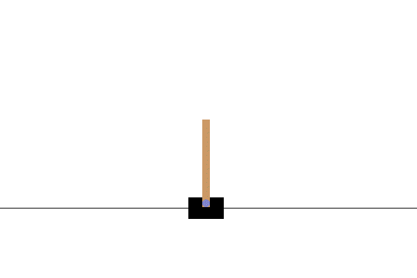
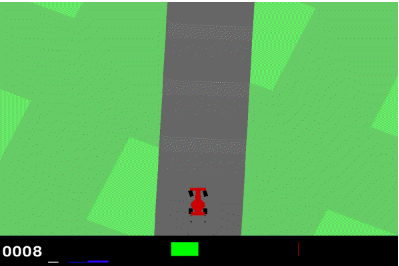
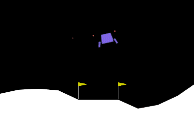
Figure 9: Cartpole, Acrobot, CarRacing, and Lunar Lander.

1. Cartpole: a pole is attached by an unactuated joint to a cart, which moves along a frictionless track. The pendulum is placed upright on the cart and the goal is to balance the pole by applying forces in the left and right direction on the cart.

2. Acrobot: a two-link pendulum system with only the second joint actuated. The task is to swing the lower link to a sufficient height in order to raise the tip of the pendulum above a target height. The environment challenges the agent’s ability to apply precise control for coordinating multiple linked joints.

3. CarRacing: The easiest control task to learn from pixels - a top-down racing environment. The generated track is random in every episode.

4. Lunar Lander: It is a classic rocket trajectory optimization problem. According to Pontryagin’s maximum principle, it is optimal to fire the engine at full throttle or turn off. This is why this environment has discrete actions: engine on or off.

E.2 MetaDrive Block Type Description

Table 3: Block Types Used in Experiments

ID	Block Type
S	Straight
C	Circular
r	InRamp
R	OutRamp
O	Roundabout
X	Intersection
y	Merge
Y	Split
T	T-Intersection

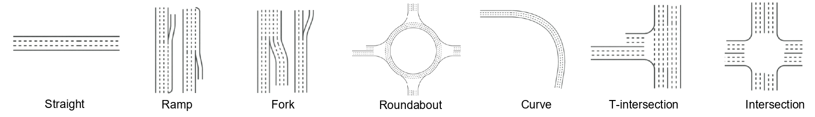
Figure 10: Various block types used in the MetaDrive environment. These blocks represent common road structures such as straight roads, ramps, forks, roundabouts, curves, T-intersections, and intersections, used for evaluating the vehicle’s path planning and decision-making capabilities.

E.3 Map Design and Testing Objectives

E.3.1 Map 1: SrOYCTRyS

This map consists of straight roads, roundabouts, intersections, T-intersections, splits, and ramps. The environment presents a highly complex combination of multiple intersections, dynamic traffic flow, and varying road structures.

Testing Objective: The focus of this environment is to evaluate the algorithm’s smooth decision-making and multi-intersection handling, mimicking human driving behavior. The challenges include adjusting vehicle paths in real-time and ensuring smooth lane transitions in the presence of complex road structures such as roundabouts and ramps.

E.3.2 Map 2: COrXSrT

This map combines circular roads, roundabouts, straight roads, intersections, ramps, and T-intersections. The environment is designed to assess the vehicle’s decision-making capabilities when dealing with continuous changes in road grades and multiple intersection types.

Testing Objective: This environment tests the algorithm’s ability to dynamically adjust to grade changes and multi-intersection interactions, replicating human-like behavior. The goal is to observe how well the algorithm adjusts vehicle speed and direction, ensuring stability in scenarios involving ramps and complex road networks.

E.3.3 Map 3: rXTSC

This map consists of ramps, intersections, T-intersections, straight roads, and circular roads. The environment simulates multiple road interactions, testing the vehicle’s path selection and stability, particularly at intersections and ramps.

Testing Objective: This environment evaluates the algorithm’s performance in handling intersections and T-junctions with real-time path selection. The challenge is to ensure human-like adaptability when encountering multiple directional options, maintaining decision stability in dynamic traffic situations.

E.3.4 Map 4: YOrSX

This map includes splits, roundabouts, straight roads, circular roads, and intersections. The environment is tailored to test the vehicle’s ability to make path decisions in high-speed settings, particularly when merging traffic and navigating through complex junctions.

Testing Objective: The map focuses on testing the vehicle’s ability to handle high-speed lane merging and dynamic path planning. The algorithm must mimic human drivers by making real-time adjustments in a high-speed environment, choosing optimal paths while maintaining speed control and safety through complex intersections and roundabouts.

E.3.5 Map 5: XTOC

This map features circular roads, T-intersections, and straight roads, creating a unique combination of continuous curves and abrupt directional changes. The environment presents the challenge of maintaining speed while negotiating tight turns and quick transitions at T-intersections.

Testing Objective: The focus is on testing the vehicle’s ability to handle sharp directional changes and maintain control during high-speed maneuvers. The algorithm needs to balance speed with precision, ensuring safe navigation through tight turns and abrupt intersections.

E.3.6 Map 6: SSSC

This map consists of three consecutive straight roads followed by a circular roundabout. It is designed to test the basic driving capabilities of the vehicle, such as lane keeping, speed control, and smooth roundabout navigation.

Testing Objective: The main challenge is to evaluate the vehicle’s ability to maintain lane stability and make appropriate speed adjustments while navigating long straight roads and transitioning into a circular roundabout. The algorithm must ensure smooth control and decision-making, simulating human-like behavior in handling both high-speed straight roads and slower, more controlled turns in the roundabout.

E.4 Environment Parameter & Agent Parameter

Table 4: Q-family vs PPO Algorithm and Environment Parameters

Parameter	Q-Family	PPO
Discrete Action Space	True
Policy	Basic_Q_network	Categorical_AC
Representation	Basic_MLP
Runner	DRL
Representation Hidden Size	[256, 256]	[512,]
Q/Actor Hidden Size	[256, 256]	[256, 256]
Critic Hidden Size	N/A	[256, 256]
Activation Function	relu	leaky_relu
Activation for Actions	N/A	tanh
Seed	123 / 321 / 666
Number of Parallels	10
Buffer Size	500,000	Horizon_Size * Parallels (128 * 10)
Batch Size	64	N/A
Horizon Size	N/A	128
Number of Epochs	N/A	4
Number of Minibatches	N/A	4
Learning Rate	0.00025
Start Greedy	1.0	N/A
End Greedy	0.01	N/A
Decay Step for Greedy	50,000	N/A
Sync Frequency	50	N/A
Training Frequency	1	N/A
Start Training Step	1,000	N/A
Running Steps	2,000,000
Use Gradient Clipping	N/A	True
Value Function Coefficient	N/A	0.25
Entropy Coefficient	N/A	0.0
Target KL Divergence	N/A	0.001
Clip Range	N/A	0.2
Clip Gradient Norm	N/A	0.5
Gamma	0.99
Use GAE	N/A	True
GAE Lambda	N/A	0.95
Use Advantage Normalization	N/A	True
Use Observation Normalization	False	True
Use Reward Normalization	False	True
Observation Normalization Range	5
Reward Normalization Range	5
Test Steps	10,000
Evaluation Interval	50,000	5,000
Test Episodes	5

Appendix F Experimental supplemental results

Table 5: We showcase the rewards of mean ± std for each algorithm in Box2D Environments

Environment/Method	CBDDQN	PPO	Duel DQN	DDQN	DQN
Cartpole	469.98 $\pm$ 20.26	427.29 $\pm$ 16.62	92.24 $\pm$ 10.56	222.14 $\pm$ 19.71	294.79 $\pm$ 16.41
Acrobot	-80.57 $\pm$ 12.63	-500.00 $\pm$ 0	-104.54 $\pm$ 40.55	-100.78 $\pm$ 21.07	-87.20 $\pm$ 14.07
CarRacing	819.08 $\pm$ 28.72	272.08 $\pm$ 27.02	-27.29 $\pm$ 6.78	788.13 $\pm$ 37.61	724.76 $\pm$ 37.17
LunarLander	158.07 $\pm$ 46.14	89.34 $\pm$ 70.44	-76.54 $\pm$ 84.85	73.04 $\pm$ 56.16	91.86 $\pm$ 70.44

Table 6: We present the rewards of mean ± std for each algorithm in Metadrive Environments

Map/Method	CBDDQN	PPO	Duel DQN	DDQN	DQN
SrOYCTRyS	130.27 $\pm$ 52.43	75.38 $\pm$ 17.80	39.20 $\pm$ 3.87	100.72 $\pm$ 39.01	105.02 $\pm$ 41.69
COrXSrT	117.90 $\pm$ 22.62	89.27 $\pm$ 19.99	53.02 $\pm$ 1.95	29.15 $\pm$ 7.03	117.18 $\pm$ 15.34
rXTSC	189.22 $\pm$ 59.94	156.74 $\pm$ 47.77	39.62 $\pm$ 3.00	185.55 $\pm$ 56.03	82.05 $\pm$ 30.27
YOrSX	232.55 $\pm$ 83.76	165.46 $\pm$ 52.43	77.65 $\pm$ 14.21	81.03 $\pm$ 24.40	221.44 $\pm$ 40.26

Table 7: We present the rewards of mean ± std for different traffic density in Metadrive XTOC map

Traffic Density/Method	CBDDQN	PPO	Duel DQN	DDQN	DQN
0.1	443.14 $\pm$ 59.63	73.90 $\pm$ 2.00	65.85 $\pm$ 8.43	151.42 $\pm$ 47.66	272.57 $\pm$ 91.25
0.3	303.15 $\pm$ 38.20	293.72 $\pm$ 56.28	67.58 $\pm$ 7.49	156.52 $\pm$ 39.27	170.73 $\pm$ 42.62
0.5	303.07 $\pm$ 40.61	256.18 $\pm$ 26.69	139.46 $\pm$ 39.78	164.34 $\pm$ 58.03	176.83 $\pm$ 56.12
0.8	161.91 $\pm$ 34.52	67.91 $\pm$ 3.42	60.71 $\pm$ 10.58	150.06 $\pm$ 36.45	147.92 $\pm$ 35.21

Table 8: We present the rewards of mean ± std for different accident probabilities in Metadrive SSSC map

Traffic Density/Method	CBDDQN	PPO	Duel DQN	DDQN	DQN
0.1	64.62 $\pm$ 10.41	-1.72 $\pm$ 0.55	40.32 $\pm$ 4.60	45.63 $\pm$ 4.56	46.73 $\pm$ 7.38
0.3	69.23 $\pm$ 6.46	45.31 $\pm$ 12.04	40.99 $\pm$ 1.83	43.42 $\pm$ 10.48	55.14 $\pm$ 9.41
0.5	69.23 $\pm$ 6.46	45.60 $\pm$ 10.24	41.12 $\pm$ 1.71	43.42 $\pm$ 10.48	55.14 $\pm$ 9.41
0.8	73.25 $\pm$ 6.78	-5.29 $\pm$ 0.16	43.78 $\pm$ 4.27	9.10 $\pm$ 3.22	55.17 $\pm$ 11.03

Appendix G Running Setting

For the Cartpole and Lunar Lander environments, the training process utilizes 1 RTX 3060 and typically runs less than 30 minutes. For the Carracing environment, we require 1 RTX 3060 and 2 hours of running. For the Metadrive environments, the training process utilizes 1 RTX 3060 and typically runs around 3-6 hours according to different complexity.

References

- Anschel et al. (2016) Oron Anschel, Nir Baram, and Nahum Shimkin. Averaged-dqn: Variance reduction and stabilization for deep reinforcement learning. In International Conference on Machine Learning, (ICML), 2016.
- Barber (2012) David Barber. Bayesian reasoning and machine learning. Cambridge University Press, 2012.
- Barber (2023) David Barber. Smoothed q-learning. arXiv preprint arXiv:2303.08631, 2023.
- Barto et al. (1989) Andrew Gehret Barto, Richard S Sutton, and CJCH Watkins. Learning and sequential decision making, volume 89. University of Massachusetts Amherst, MA, 1989.
- Bas-Serrano et al. (2021) Joan Bas-Serrano, Sebastian Curi, Andreas Krause, and Gergely Neu. Logistic q-learning. In International conference on artificial intelligence and statistics, pp. 3610–3618. PMLR, 2021.
- Botvinick et al. (2020) Matthew Botvinick, Jane X Wang, Will Dabney, Kevin J Miller, and Zeb Kurth-Nelson. Deep reinforcement learning and its neuroscientific implications. Neuron, 107(4):603–616, 2020.
- Carroll et al. (2019) Micah Carroll, Rohin Shah, Mark K Ho, Tom Griffiths, Sanjit Seshia, Pieter Abbeel, and Anca Dragan. On the utility of learning about humans for human-ai coordination. volume 32, 2019.
- Doya (2007) Kenji Doya. Bayesian brain: Probabilistic approaches to neural coding. MIT press, 2007.
- Fujimoto et al. (2018) Scott Fujimoto, Herke Hoof, and David Meger. Addressing function approximation error in actor-critic methods. In International conference on machine learning, pp. 1587–1596. PMLR, 2018.
- Garg et al. (2023) Divyansh Garg, Joey Hejna, Matthieu Geist, and Stefano Ermon. Extreme q-learning: Maxent rl without entropy. arXiv preprint arXiv:2301.02328, 2023.
- Gershman et al. (2015) Samuel J Gershman, Eric J Horvitz, and Joshua B Tenenbaum. Computational rationality: A converging paradigm for intelligence in brains, minds, and machines. Science, 349(6245):273–278, 2015.
- Gigerenzer et al. (1991) Gerd Gigerenzer, Ulrich Hoffrage, and Heinz Kleinbölting. Probabilistic mental models: a brunswikian theory of confidence. Psychological review, 98(4):506, 1991.
- Guss et al. (2021) William Hebgen Guss, Stephanie Milani, Nicholay Topin, Brandon Houghton, Sharada Mohanty, Andrew Melnik, Augustin Harter, Benoit Buschmaas, Bjarne Jaster, Christoph Berganski, et al. Towards robust and domain agnostic reinforcement learning competitions: Minerl 2020. In NeurIPS 2020 Competition and Demonstration Track, pp. 233–252. PMLR, 2021.
- Hasselt (2010) Hado Hasselt. Double q-learning. Advances in neural information processing systems, 23, 2010.
- Hastie & Dawes (2009) Reid Hastie and Robyn M Dawes. Rational choice in an uncertain world: The psychology of judgment and decision making. Sage Publications, 2009.
- Hogarth & Einhorn (1992) Robin M Hogarth and Hillel J Einhorn. Order effects in belief updating: The belief-adjustment model. Cognitive psychology, 24(1):1–55, 1992.
- Hu et al. (2021) Hengyuan Hu, Adam Lerer, Brandon Cui, Luis Pineda, Noam Brown, and Jakob Foerster. Off-belief learning. In International Conference on Machine Learning, (ICML), pp. 4369–4379. PMLR, 2021.
- Hui et al. (2023) David Yu-Tung Hui, Aaron Courville, and Pierre-Luc Bacon. Double gumbel q-learning. In Thirty-seventh Conference on Neural Information Processing Systems, 2023. URL https://openreview.net/forum?id=UdaTyy0BNB.
- Hui et al. (2024) David Yu-Tung Hui, Aaron C Courville, and Pierre-Luc Bacon. Double gumbel q-learning. Advances in Neural Information Processing Systems, 36, 2024.
- Ikotun et al. (2022) Abiodun Motunrayo Ikotun, Ezugwu E. Absalom, Laith Mohammad Abualigah, Belal Abuhaija, and Heming Jia. K-means clustering algorithms: A comprehensive review, variants analysis, and advances in the era of big data. Inf. Sci., 622:178–210, 2022.
- Kochenderfer (2015) Mykel J Kochenderfer. Decision making under uncertainty: theory and application. MIT press, 2015.
- Li et al. (2022) Quanyi Li, Zhenghao Peng, Lan Feng, Qihang Zhang, Zhenghai Xue, and Bolei Zhou. Metadrive: Composing diverse driving scenarios for generalizable reinforcement learning. IEEE Transactions on Pattern Analysis and Machine Intelligence, 2022.
- Liu et al. (2024) Rui Liu, Xuanzhen Xu, Yuwei Shen, Armando Zhu, Chang Yu, Tianjian Chen, and Ye Zhang. Enhanced detection classification via clustering SVM for various robot collaboration task. CoRR, abs/2405.03026, 2024.
- Liu et al. (2023) Wenzhang Liu, Wenzhe Cai, Kun Jiang, Guangran Cheng, Yuanda Wang, Jiawei Wang, Jingyu Cao, Lele Xu, Chaoxu Mu, and Changyin Sun. Xuance: A comprehensive and unified deep reinforcement learning library. arXiv preprint arXiv:2312.16248, 2023.
- Mao et al. (2020) Hangyu Mao, Wulong Liu, Jianye Hao, Jun Luo, Dong Li, Zhengchao Zhang, Jun Wang, and Zhen Xiao. Neighborhood cognition consistent multi-agent reinforcement learning. In Proceedings of the AAAI conference on artificial intelligence, volume 34, pp. 7219–7226, 2020.
- Mao et al. (2022) Hangyu Mao, Chao Wang, Xiaotian Hao, Yihuan Mao, Yiming Lu, Chengjie Wu, Jianye Hao, Dong Li, and Pingzhong Tang. Seihai: A sample-efficient hierarchical ai for the minerl competition. In Distributed Artificial Intelligence: Third International Conference, DAI 2021, Shanghai, China, December 17–18, 2021, Proceedings 3, pp. 38–51. Springer, 2022.
- Markman & Ross (2003) Arthur B Markman and Brian H Ross. Category use and category learning. Psychological bulletin, 129(4):592, 2003.
- McAleer et al. (2024) Stephen McAleer, Gabriele Farina, Gaoyue Zhou, Mingzhi Wang, Yaodong Yang, and Tuomas Sandholm. Team-psro for learning approximate tmecor in large team games via cooperative reinforcement learning. Advances in Neural Information Processing Systems, 36, 2024.
- Melo (2001) Francisco S Melo. Convergence of q-learning: A simple proof. Institute Of Systems and Robotics, Tech. Rep, pp. 1–4, 2001.
- Mnih et al. (2013) Volodymyr Mnih, Koray Kavukcuoglu, David Silver, Alex Graves, Ioannis Antonoglou, Daan Wierstra, and Martin A. Riedmiller. Playing atari with deep reinforcement learning. CoRR, abs/1312.5602, 2013.
- Mnih et al. (2015) Volodymyr Mnih, Koray Kavukcuoglu, David Silver, Andrei A Rusu, Joel Veness, Marc G Bellemare, Alex Graves, Martin Riedmiller, Andreas K Fidjeland, Georg Ostrovski, et al. Human-level control through deep reinforcement learning. nature, 518(7540):529–533, 2015.
- Mongin (1998) Philippe Mongin. Expected utility theory. 1998.
- O’Donoghue (2021) Brendan O’Donoghue. Variational bayesian reinforcement learning with regret bounds. Advances in Neural Information Processing Systems, 34:28208–28221, 2021.
- Parberry (2017) Ian Parberry. Introduction to Game Physics with Box2D. CRC Press, 2017.
- Peterson & Beach (1967) Cameron R Peterson and Lee Roy Beach. Man as an intuitive statistician. Psychological bulletin, 68(1):29, 1967.
- Ren et al. (2021) Zhizhou Ren, Guangxiang Zhu, Hao Hu, Beining Han, Jianglun Chen, and Chongjie Zhang. On the estimation bias in double q-learning. Advances in Neural Information Processing Systems, 34:10246–10259, 2021.
- Rosch & Mervis (1975) Eleanor Rosch and Carolyn B Mervis. Family resemblances: Studies in the internal structure of categories. Cognitive psychology, 7(4):573–605, 1975.
- Rudin (2019) Cynthia Rudin. Stop explaining black box machine learning models for high stakes decisions and use interpretable models instead. Nature machine intelligence, 1(5):206–215, 2019.
- Silver et al. (2016) David Silver, Aja Huang, Chris J Maddison, Arthur Guez, Laurent Sifre, George Van Den Driessche, Julian Schrittwieser, Ioannis Antonoglou, Veda Panneershelvam, Marc Lanctot, et al. Mastering the game of go with deep neural networks and tree search. nature, 529(7587):484–489, 2016.
- Singh et al. (2000) Satinder Singh, Tommi Jaakkola, Michael L Littman, and Csaba Szepesvári. Convergence results for single-step on-policy reinforcement-learning algorithms. Machine learning, 38:287–308, 2000.
- Soltani & Izquierdo (2019) Alireza Soltani and Alicia Izquierdo. Adaptive learning under expected and unexpected uncertainty. Nature Reviews Neuroscience, 20(10):635–644, 2019.
- Sutton & Barto (2018) Richard S Sutton and Andrew G Barto. Reinforcement learning: An introduction. MIT press, 2018.
- Sutton et al. (1999) Richard S Sutton, Andrew G Barto, et al. Reinforcement learning. Journal of Cognitive Neuroscience, 11(1):126–134, 1999.
- Thrun & Schwartz (2014) Sebastian Thrun and Anton Schwartz. Issues in using function approximation for reinforcement learning. In Proceedings of the 1993 connectionist models summer school, 2014.
- Towers et al. (2024) Mark Towers, Ariel Kwiatkowski, Jordan Terry, John U Balis, Gianluca De Cola, Tristan Deleu, Manuel Goulão, Andreas Kallinteris, Markus Krimmel, Arjun KG, et al. Gymnasium: A standard interface for reinforcement learning environments. arXiv preprint arXiv:2407.17032, 2024.
- Tversky & Kahneman (1992) Amos Tversky and Daniel Kahneman. Advances in prospect theory: Cumulative representation of uncertainty. Journal of Risk and uncertainty, 5:297–323, 1992.
- Wang et al. (2021) Hang Wang, Sen Lin, and Junshan Zhang. Adaptive ensemble q-learning: Minimizing estimation bias via error feedback. Advances in neural information processing systems, 34:24778–24790, 2021.
- Watkins & Dayan (1992) Christopher JCH Watkins and Peter Dayan. Q-learning. Machine learning, 8:279–292, 1992.
- Watkins (1989) Christopher John Cornish Hellaby Watkins. Learning from delayed rewards. 1989.
- Weng et al. (2020) Wentao Weng, Harsh Gupta, Niao He, Lei Ying, and R Srikant. The mean-squared error of double q-learning. Advances in Neural Information Processing Systems, 33:6815–6826, 2020.
- Wu et al. (2024) Jingda Wu, Haohan Yang, Lie Yang, Yi Huang, Xiangkun He, and Chen Lv. Human-guided deep reinforcement learning for optimal decision making of autonomous vehicles. IEEE Transactions on Systems, Man, and Cybernetics: Systems, 2024.
- Xu et al. (2020) Jie Xu, Yunsheng Tian, Pingchuan Ma, Daniela Rus, Shinjiro Sueda, and Wojciech Matusik. Prediction-guided multi-objective reinforcement learning for continuous robot control. In International conference on machine learning, pp. 10607–10616. PMLR, 2020.
- Zhang et al. (2024) Bin Zhang, Hangyu Mao, Lijuan Li, Zhiwei Xu, Dapeng Li, Rui Zhao, and Guoliang Fan. Sequential asynchronous action coordination in multi-agent systems: A stackelberg decision transformer approach. In Forty-first International Conference on Machine Learning, 2024.
- Zhang et al. (2021) Mingtian Zhang, Peter Hayes, Tim Z Xiao, Andi Zhang, and David Barber. Solipsistic reinforcement learning. In International Conference on Learning Representations workshop, 2021.