Worst-Case Values of Target Semi-Variances With Applications to Robust Portfolio Selection

Abstract

The expected regret and target semi-variance are two of the most important risk measures for downside risk. When the distribution of a loss is uncertain, and only partial information of the loss is known, their worst-case values play important roles in robust risk management for finance, insurance, and many other fields. Jagannathan (1977) derived the worst-case expected regrets when only the mean and variance of a loss are known and the loss is arbitrary, symmetric, or non-negative. While Chen et al. (2011) obtained the worst-case target semi-variances under similar conditions but focusing on arbitrary losses. In this paper, we first complement the study of Chen et al. (2011) on the worst-case target semi-variances and derive the closed-form expressions for the worst-case target semi-variance when only the mean and variance of a loss are known and the loss is symmetric or non-negative. Then, we investigate worst-case target semi-variances over uncertainty sets that represent undesirable scenarios faced by an investors. Our methods for deriving these worst-case values are different from those used in Jagannathan (1977) and Chen et al. (2011). As applications of the results derived in this paper, we propose robust portfolio selection methods that minimize the worst-case target semi-variance of a portfolio loss over different uncertainty sets. To explore the insights of our robust portfolio selection methods, we conduct numerical experiments with real financial data and compare our portfolio selection methods with several existing portfolio selection models related to the models proposed in this paper.

Keywords: Downside risk; target semi-variance; worst-case risk measure; distribution uncertainty; distributionally robust optimization; robust portfolio selection.

1 Introduction

Assume that $X$ is a random variable denoting the loss of an investment portfolio. Hence, in this paper, positive values of $X$ represent losses and negative values of $X$ represent gains or returns. The manager of an investment portfolio often has a target return $-t$ or equivalently a threshold loss $t$. Thus, the loss function $(X-t)_{+}$ represents the downside risk/loss of the portfolio, while $(-X-(-t))_{+}=(X-t)_{-}$ denotes the excess profit of the portfolio over the target return. Here and throughout this paper, $(x)_{+}=\max\{x,0\}$ and $(x)_{-}=\max\{-x,0\}$ for any $x\in\mathbb{R}=(-\infty,\infty)$. Two important quantities of the downside risk $(X-t)_{+}$ are the first moment $\mathbb{E}[(X-t)_{+}]$ that measures the expected loss above the threshold loss $t$ and the second moment $\mathbb{E}[(X-t)_{+}^{2}]$ that quantifies the dispersion of the loss that exceeds the threshold loss $t$. In the literature, the two moments are often called the first-order and second-order upper partial moments, respectively. In addition, the first moment $\mathbb{E}[(X-t)_{+}]$ is also referred to as the expected regret or target shortfall (see, e.g., Testuri and Uryasev (2004), Krokhmal et al. (2011)), while the second moment $\mathbb{E}[(X-t)_{+}^{2}]$ is also referred to as the target semi-variance (see, e.g., Rohatgi (2011)). If the target return is equal to the expected return, namely, $t=\mathbb{E}[X]$, the target semi-variance $\mathbb{E}[(X-\mathbb{E}[X])_{+}^{2}]$ is called the semi-variance of the loss $X$. Both of the expected regret and the target semi-variance are important risk measures of the downside risk and have been extensively used in finance, insurance, operations research, and many other fields.

If the ‘true’ distribution of the loss $X$ is known, the expected regret $\mathbb{E}[(X-t)_{+}]$ and the target semi-variance $\mathbb{E}[(X-t)_{+}^{2}]$ can be calculated analytically or numerically. However, in practice, the ‘true’ distribution of $X$ is often unknown. A decision maker may have only partial information on $X$ such as the mean and variance of $X$. If only partial information on $X$ is available and the possible distributions of $X$ belong to a distribution set ${\cal L}$, called an uncertainty set for $X$, a decision maker is often interested in $\sup_{F\in{\cal L}}\mathbb{E}^{F}[(X-t)_{+}]$ and $\sup_{F\in{\cal L}}\mathbb{E}^{F}[(X-t)^{2}_{+}]$, which are respectively called the worst-case expected regret and the worst-case target semi-variance over the uncertainty set ${\cal L}$. Here and throughout this paper, for a function $h$ defined on $\mathbb{R}$ and a risk measure $\rho$, such as expectation $\mathbb{E}$, variance $\rm Var$, and conditional value-at-risk CVaR, $\rho^{F}[h(X)]$ means that the risk measure of $\rho(h(X))$ is calculated under the distribution $F$ if the distribution of $X$ is $F$. In the literature, for a random variable $X$ and a loss/cost function $h$, when the ‘true’ distribution of $X$ is unknown or uncertain but is assumed to be in an uncertainty set ${\cal L}$, the optimization problem of

$$\sup_{F\in{\cal L}}\rho^{F}[h(X)]$$ (1.1)

is called a distributionally robust optimization (DRO) problem, and if there exists a distribution $F^{*}\in{\cal L}$ such that $\sup_{F\in{\cal L}}\rho^{F}[h(X)]=\rho^{F^{*}}[h(X)]$, such a distribution is called a worst-case distribution. The DRO problem (1.1) and its applications have been extensively studied in the literature of finance, insurance, operations research, and many other fields. For instance, Jagannathan (1977) investigated problem (1.1) when $\rho=\mathbb{E}$, $h(x)=(x-t)_{+}$, ${\cal L}$ is a set containing distributions with the given first two moments, and $X$ is an arbitrary, symmetric or non-negative random variable. Zuluaga et al. (2009) considered problem (1.1) when $\rho=\mathbb{E}$, $h(x)=(x-t)_{+}$, ${\cal L}$ is a set containing distributions with the given first three moments. Chen et al. (2011) studied problem (1.1) when $\rho=\mathbb{E}$, $h(x)=(x-t)_{-}^{2}$, and ${\cal L}$ is a set containing distributions with the given first two moments. Tang and Yang (2023) discussed problem (1.1) when $h(x)=x^{m}$ or $(x-t)^{m}_{+}$, $m=1,2,...,$ and ${\cal L}$ is a set containing distributions satisfying a distance constraint to a reference distribution. Cai et al. (2024) studied problem (1.1) when $\rho$ is a distortion risk measure, $h(x)=(x-t)_{+}$, and ${\cal L}$ is a set containing distributions satisfying a distance constraint to a reference distribution and constraints on first two moments. For the studies and applications of the DRO problem (1.1) with other forms of the function $h$ and the risk measure $\rho$, we refer to Ben-Tal and Nemirovski (1998), Bertsimas and Popescu (2002), Ghaoui et al. (2003), Hürlimann (2005), Natarajan et al. (2008), Zhu and Fukushima (2009), Zhu et al. (2009), Asimit et al. (2017), Pflug et al. (2017), Li (2018), Kang et al. (2019), Liu and Mao (2022), Bernard et al. (2023) , Cai et al. (2023), and the references therein.

In many DRO problems, it is assumed that the mean and variance or second moment of a random variable $X$ are the only known information on the distribution of $X$, which correspond to the following uncertainty set

$$\mathcal{L}(\mu,\sigma) =\big{\{}F\in\mathcal{F}(\mathbb{R}):\,\int^{\infty}_{-\infty}x\,\mathrm{d}F(x)=\mu,\int^{\infty}_{-\infty}x^{2}\,\mathrm{d}F(x)=\mu^{2}+\sigma^{2}\big{\}}$$

$$=\big{\{}F\in\mathcal{F}(\mathbb{R}):\,\mathbb{E}^{F}[X]=\mu,\,\mathbb{E}^{F}[X^{2}]=\mu^{2}+\sigma^{2}\big{\}},$$ (1.2)

where $\mathcal{F}(\mathbb{R})$ is the set of all the distributions defined on $\mathbb{R}$. In practice, a decision maker may have additional information on the distribution of $X$ besides its mean and variance. In finance, a decision maker may notice that the loss data have the symmetric features. For instance, Figure 1 displays the histograms of daily losses of the stocks of Apple, Bank of America, Johnson & Johnson, and Tesla. The daily losses of these stocks exhibit a high degree of symmetry.

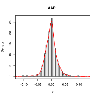
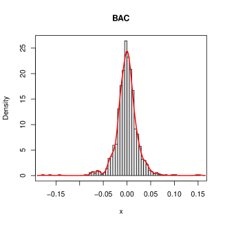
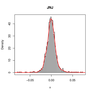
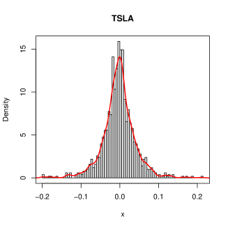
Figure 1: Histograms of daily losses of the stocks of Apple (AAPL), Bank of America (BAC), Johnson & Johnson (JNJ) and Tesla (TSLA). The data used for this figure covers a four-year period from January 2, 2019, to January 2, 2023, and includes 1007 observations of daily losses from Yahoo! Finance.

In fact, in many portfolio selection researches, the daily losses of the underlying assets are assumed to have multivariate symmetric distributions such as multivariate normal distributions, multivariate $t$-distributions, multivariate elliptical distributions, and so on. See, for example, Owen and Rabinovitch (1983), Buckley et al. (2008), Hu and Kercheval (2010), Fang (2018), and the references therein.

In addition, in insurance, loss random variables often are the amounts and numbers of insurance claims that are non-negative random variables. Hence, the following two uncertainty sets

$$\mathcal{L}_{S}(\mu,\sigma)=\big{\{}F\in\mathcal{L}(\mu,\sigma):\ \text{$F$ is symmetric}\big{\}},$$ (1.3)

$$\mathcal{L}^{+}(\mu,\sigma)=\big{\{}F\in\mathcal{L}(\mu,\sigma):\ F(0-)=0\big{\}},$$ (1.4)

are also interesting in the study of DRO problems. In this paper, the formal definitions of symmetric distributions are given in Definitions 2.1 and 5.1, and a non-negative distribution means that $F(0-)=\mathbb{P}\{X<0\}=0$ or $F$ is a distribution of a non-negative random variable $X$.

The closed-form expressions for $\sup_{F\in{\cal L}}\mathbb{E}[(X-t)_{+}]$ have been derived in Jagannathan (1977) when ${\cal L}$ is one of the three uncertainty sets $\mathcal{L}(\mu,\sigma)$ $\mathcal{L}_{S}(\mu,\sigma)$, and $\mathcal{L}^{+}(\mu,\sigma)$. The closed-form expression for $\sup_{F\in{\cal L}}\mathbb{E}[(X-t)^{2}_{-}]$ has been obtained in Chen et al. (2011) when ${\cal L}=\mathcal{L}(\mu,\sigma)$. To the best of our knowledge, the worst-case values of $\mathbb{E}[(X-t)^{2}_{+}]$ over the uncertainty sets $\mathcal{L}_{S}(\mu,\sigma)$ and $\mathcal{L}^{+}(\mu,\sigma)$ have not been solved. As discussed later in this paper, the methods and proofs used in Jagannathan (1977) and Chen et al. (2011) do not apply for the worst-case values of $\mathbb{E}[(X-t)^{2}_{+}]$ over the uncertainty sets $\mathcal{L}_{S}(\mu,\sigma)$ and $\mathcal{L}^{+}(\mu,\sigma)$.

In this paper, first, we complement the study of Chen et al. (2011) on worst-case values of the target semi-variance and obtain the closed-form expressions for the worst-case values of the target semi-variance over the uncertainty sets $\mathcal{L}_{S}(\mu,\sigma)$ and $\mathcal{L}^{+}(\mu,\sigma)$. Second, motivated by the classical mean-variance (M-V) portfolio selection model, we discuss the applications of the worst-case target semi-variance in portfolio selection problems and propose portfolio selection models based on expected excess profit-target semi-variance (EEP-TSV). These models aim to minimize the worst-case target semi-variance of portfolio loss over undesirable scenarios where the expected excess profit does not meet a desirable minimum level $\lambda$. As illustrated in Section 5, these EEP-TSV-based portfolio selection models can be transformed into problems that minimize the worst-case target semi-variance of portfolio loss over the following uncertain sets:

$$\mathcal{L}_{\lambda}(\mu,\sigma) =\big{\{}F\in\mathcal{L}(\mu,\sigma):\ \mathbb{E}^{F}[(X-t)_{-}]\leqslant\lambda\big{\}},$$ (1.5)

$$\mathcal{L}_{S,\lambda}(\mu,\sigma) =\big{\{}F\in\mathcal{L}(\mu,\sigma):\ \text{$F$ is symmetric and}\ \mathbb{E}^{F}[(X-t)_{-}]\leqslant\lambda\},$$ (1.6)

$$\mathcal{L}^{+}_{\lambda}(\mu,\sigma) =\big{\{}F\in\mathcal{L}(\mu,\sigma):\ F(0-)=0\ \text{and}\ \mathbb{E}^{F}[(X-t)_{-}]\leqslant\lambda\big{\}}.$$ (1.7)

Note that, in this paper, $\mathbb{E}^{F}[(X-t)_{-}]$ denotes the expected excess profit. Thus, if $\lambda>0$ represents a desirable minimum level for the expected excess profit, then $\mathbb{E}^{F}[(X-t)_{-}]\leqslant\lambda$ in (1.5)-(1.7) indicates that the expected excess profit does not meet the desirable minimum level, which is an undesirable scenario for an investor. Conversely, $\mathbb{E}^{F}[(X-t)_{-}]>\lambda$ represents a desirable scenario for an investor. In fact, for any uncertainty set $\mathcal{L}$ for the loss random variable $X$, it holds that

$$\mathcal{L}=\big{\{}F\in\mathcal{L}:\ \mathbb{E}^{F}[(X-t)_{-}]\leqslant\lambda\big{\}}\,\cup\,\big{\{}F\in\mathcal{L}:\ \mathbb{E}^{F}[(X-t)_{-}]>\lambda\big{\}}.$$

An investor is primarily concerned with the undesirable scenario where $\mathbb{E}^{F}[(X-t)_{-}]\leqslant\lambda$ and with the worst-case values over the set $\big{\{}F\in\mathcal{L}:\ \mathbb{E}^{F}[(X-t)_{-}]\leqslant\lambda\big{\}}$ such as those defined in (1.5)-(1.7). In addition, the uncertainty sets $\mathcal{L}(\mu,\sigma)$, $\mathcal{L}_{S}(\mu,\sigma),$ and $\mathcal{L}^{+}(\mu,\sigma)$ can be treated as the limiting cases of $\mathcal{L}_{\lambda}(\mu,\sigma)$, $\mathcal{L}_{S,\lambda}(\mu,\sigma)$, and $\mathcal{L}^{+}_{\lambda}(\mu,\sigma)$, respectively, as $\lambda\to\infty$.

The uncertainty sets $\mathcal{L}_{S}(\mu,\sigma)$, $\mathcal{L}^{+}(\mu,\sigma)$, $\mathcal{L}_{\lambda}(\mu,\sigma)$, and $\mathcal{L}_{S,\lambda}(\mu,\sigma)$ have more constraints than $\mathcal{L}(\mu,\sigma)$. Finding the worst-case values of $\mathbb{E}[(X-t)^{2}_{+}]$ over the uncertainty sets $\mathcal{L}_{S}(\mu,\sigma)$, $\mathcal{L}^{+}(\mu,\sigma)$, $\mathcal{L}_{\lambda}(\mu,\sigma)$, $\mathcal{L}_{S,\lambda}(\mu,\sigma)$ is a challenging question, in particular, over the uncertainty sets $\mathcal{L}_{S}(\mu,\sigma)$ and $\mathcal{L}_{S,\lambda}(\mu,\sigma)$. The main method used in this paper for finding these worst-case values is to reformulate these infinite-dimensional optimization problems to finite-dimensional optimization problems and then solve the finite-dimensional optimization problems to obtain the closed-form expressions for the worst-case values.

The rest of paper is structured as follows. In Section 2, we give the preliminaries of the worst-case values of the expected regret and target semi-variance and describe our motivation for studying the worst-case target semi-variance. In Section 3, we derive the closed-form expressions for the worst-case target semi-variance over the uncertainty set $\mathcal{L}_{S}(\mu,\sigma)$. In Section 4, we provide the closed-form expressions for worst-case target semi-variances over undesirable scenarios, which are worst-case target semi-variances over the uncertainty sets $\mathcal{L}_{\lambda}(\mu,\sigma)$ and $\mathcal{L}_{S,\lambda}(\mu,\sigma)$. In Section 5, we propose robust portfolio selection models that minimize the target semi-variance under the different uncertainty sets discussed above. In Section 6, we use the real finance data to compare the investment performances of our portfolio selection methods with several existing portfolio selection models related to the models proposed in this paper. In Section 7, we give concluding remarks. The proofs of the main results in this paper are presented in the appendix, which is located in Section 8.

2 Preliminary and motivation

Definition 2.1.

The distribution $F$ of a random variable $X$ is said to be symmetric if there exists a constant $a$ such that $\mathbb{P}(X-a>x)=\mathbb{P}(X-a<-x)$, under the distribution $F$, for all $x\in\mathbb{R}$. If such a constant $a$ exists, random variable $X$ or its distribution is said to be symmetric about $a$. $\Box$

Intuitively, random variable $X$ is symmetric about $a$ if and only if $X-a$ is symmetric about the origin of $\mathbb{R}$. Examples of continuous symmetric distributions include the Cauchy distribution, normal distribution, $t$-distribution, uniform distribution, logistic distribution, and many others. Examples of discrete symmetric distributions include discrete uniform distribution, $k$-point symmetric distribution (where $k\geqslant 2$ is an integer), and many others. In addition, a degenerate distribution is also symmetric according to Definition 2.1.

To give a detailed review of the known results about the worst-case values $\sup_{F\in{\cal L}}\mathbb{E}^{F}[(X-t)_{+}]$ and $\sup_{F\in{\cal L}}\mathbb{E}^{F}[(X-t)^{2}_{+}]$ and illustrate our motivation for studying the worst-case target semi-variance, we state the results of Jagannathan (1977) and Chen et al. (2011) about these worst-case values and give remarks on these results and their proofs below.

Proposition 2.1.

(Jagannathan (1977)) For any $\mu,t\in\mathbb{R}$ and $\sigma\in\mathbb{R}^{+}=(0,\infty)$, if the uncertainty set of random variable $X$ is $\mathcal{L}(\mu,\sigma)$, then

$$\sup_{F\in\mathcal{L}(\mu,\sigma)}\mathbb{E}^{F}[(X-t)_{+}]=\frac{1}{2}\left(\mu-t+\sqrt{\sigma^{2}+(\mu-t)^{2}}\right).$$ (2.1)

If the uncertainty set of $X$ is $\mathcal{L}_{S}(\mu,\sigma)$, then

$$\sup_{F\in\mathcal{L}_{S}(\mu,\sigma)}\mathbb{E}^{F}[(X-t)_{+}]=\begin{cases}\frac{8(\mu-t)^{2}+\sigma^{2}}{8(\mu-t)},&t<\mu-\frac{\sigma}{2},\\ \frac{1}{2}(\mu+\sigma-t),&\mu-\frac{\sigma}{2}\leqslant t<\mu+\frac{\sigma}{2},\\ \frac{\sigma^{2}}{8(t-\mu)},&t\geqslant\mu+\frac{\sigma}{2}.\end{cases}$$ (2.2)

If the uncertainty set of $X$ is $\mathcal{L}^{+}(\mu,\sigma)$ and $\mu>0$, then

$$\sup_{F\in\mathcal{L}^{+}(\mu,\sigma)}\mathbb{E}^{F}[(X-t)_{+}]=\begin{cases}\mu-t,&t<0,\\ \mu-\frac{\mu^{2}t}{\sigma^{2}+\mu^{2}},&0\leqslant t<\frac{\sigma^{2}+\mu^{2}}{2\mu},\\ \frac{1}{2}\left(\mu-t+\sqrt{\sigma^{2}+(\mu-t)^{2}}\right),&t\geqslant\frac{\sigma^{2}+\mu^{2}}{2\mu}.\end{cases}$$ (2.3)

Remark 2.1.

The main idea of Jagannathan (1977)’s proof for Proposition 2.1 as follows: First apply Cauchy-Schwarz’s inequality for $\mathbb{E}[(X-t)_{+}]$ or start with $(\mathbb{E}[(X-t)_{+}])^{2}=\big{(}\int^{\infty}_{t}(x-t)\,\mathrm{d}F(x)\big{)}^{2}\leqslant\int^{\infty}_{t}\,\mathrm{d}F(x)\,\int^{\infty}_{t}(x-t)^{2}\,\mathrm{d}F(x)$ and obtain the sharp upper bound for $\sup_{F\in{\cal L}}\int^{\infty}_{t}\,\mathrm{d}F(x)\,\int^{\infty}_{t}(x-t)^{2}\,\mathrm{d}F(x)$, and then verify that the upper bound is also the sharp bound for $\sup_{F\in{\cal L}}\mathbb{E}^{F}[(X-t)_{+}]$. We point out that the arguments and proofs used in Jagannathan (1977) for Proposition 2.1 do not work for the worst-case values of $\sup_{F\in{\cal L}}\mathbb{E}^{F}[(X-t)^{2}_{+}]$ when ${\cal L}$ is any of the uncertainty sets $\mathcal{L}(\mu,\sigma)$, $\mathcal{L}_{S}(\mu,\sigma)$, and $\mathcal{L}^{+}(\mu,\sigma)$. If fact, if one applies Cauchy-Schwarz’s inequality to $\mathbb{E}[(X-t)^{2}_{+}]$, one obtains $(\mathbb{E}[(X-t)^{2}_{+}])^{2}=\big{(}\int^{\infty}_{t}(x-t)^{2}\,\mathrm{d}F(x)\big{)}^{2}\leqslant\int^{\infty}_{t}\,\mathrm{d}F(x)\,\int^{\infty}_{t}(x-t)^{4}\,\mathrm{d}F(x).$ However, the upper bound $\int^{\infty}_{t}\,\mathrm{d}F(x)\,\int^{\infty}_{t}(x-t)^{4}\,\mathrm{d}F(x)$ does not provide any useful information for $(\mathbb{E}[(X-t)^{2}_{+}])^{2}$ since $\int^{\infty}_{t}(x-t)^{4}\,\mathrm{d}F(x)$ may be equal to $\infty$ when $F$ is in any of the sets $\mathcal{L}(\mu,\sigma)$, $\mathcal{L}_{S}(\mu,\sigma)$, and $\mathcal{L}^{+}(\mu,\sigma)$. $\Box$

Note that for any $x\in\mathbb{R}$, $(x)_{+}-(x)_{-}=x$, $(x)^{2}_{+}+(x)_{-}^{2}=x^{2}$, and $(x)_{+}=(-x)_{-}$. Hence, for any $t\in\mathbb{R}$, if $\mathcal{L}^{*}(\mu,\sigma)\subset{\cal F}(\mathbb{R})$ is a set of distributions satisfying that for any $F\in\mathcal{L}^{*}(\mu,\sigma)$, $\mathbb{E}^{F}[X]=\mu$ and $\mathbb{E}^{F}[X^{2}]=\mu^{2}+\sigma^{2}$, then

$$\sup_{F\in\mathcal{L}^{*}(\mu,\sigma)}\mathbb{E}^{F}[(X-t)_{+}] \ =\ \sup_{F\in\mathcal{L}^{*}(\mu,\sigma)}\mathbb{E}^{F}[(X-t)_{-}]+\mu-t,$$ (2.4)

$$\inf_{F\in\mathcal{L}^{*}(\mu,\sigma)}\mathbb{E}^{F}[(X-t)_{+}] \ =\ \inf_{F\in\mathcal{L}^{*}(\mu,\sigma)}\mathbb{E}^{F}[(X-t)_{-}]+\mu-t,$$ (2.5)

$$\sup_{F\in\mathcal{L}^{*}(\mu,\sigma)}\mathbb{E}^{F}[(X-t)_{+}^{2}] \ =\ \sigma^{2}+(t-\mu)^{2}\,-\,\inf_{F\in\mathcal{L}^{*}(\mu,\sigma)}\mathbb{E}^{F}[(X-t)^{2}_{-}],$$ (2.6)

$$\inf_{F\in\mathcal{L}^{*}(\mu,\sigma)}\mathbb{E}^{F}[(X-t)_{+}^{2}] \ =\ \sigma^{2}+(t-\mu)^{2}\,-\,\sup_{F\in\mathcal{L}^{*}(\mu,\sigma)}\mathbb{E}^{F}[(X-t)^{2}_{-}].$$ (2.7)

In addition, for random variable $X$, the conditions of $\mathbb{E}[X]=\mu$ and $\mathbb{E}[X^{2}]=\mu^{2}+\sigma^{2}$ are equivalent to the conditions of $\mathbb{E}[-X]=-\mu$ and $\mathbb{E}[(-X)^{2}]=\mu^{2}+\sigma^{2}$, and the condition that $X$ is symmetric about $\mu$ is equivalent to the condition that $-X$ is symmetric about $-\mu$. Hence, if $\mathcal{L}_{0}(\mu,\sigma)$ is one of the sets $\mathcal{L}(\mu,\sigma)$ and $\mathcal{L}_{S}(\mu,\sigma)$, then for $k=1,2$,

$$\sup_{F\in\mathcal{L}_{0}(\mu,\sigma)}\mathbb{E}^{F}[(X-t)^{k}_{+}] =\sup_{F\in\mathcal{L}_{0}(-\mu,\sigma)}\mathbb{E}^{F}[(X-(-t))^{k}_{-})],$$ (2.8)

$$\inf_{F\in\mathcal{L}_{0}(\mu,\sigma)}\mathbb{E}^{F}[(X-t)^{k}_{+})] =\inf_{F\in\mathcal{L}_{0}(-\mu,\sigma)}\mathbb{E}^{F}[(X-(-t))^{k}_{-})].$$ (2.9)

We also point out that the downside risk of an investment portfolio is $(t-X)_{+}=(X-t)_{-}$ if $X$ represents the return or gain of the portfolio and $t$ is the target return.

Proposition 2.2.

(Chen et al. (2011)) For any $\mu,t\in\mathbb{R}$ and $\sigma\in\mathbb{R}^{+}$, we have

$$\sup_{F\in\mathcal{L}(\mu,\sigma)}\mathbb{E}^{F}[(X-t)^{2}_{-}] =\sigma^{2}+(t-\mu)^{2}_{+},$$ (2.10)

$$\sup_{F\in\mathcal{L}(\mu,\sigma)}\mathbb{E}^{F}[(X-t)_{+}^{2}] =\sigma^{2}+(\mu-t)_{+}^{2}.$$ (2.11)

Remark 2.2.

Formula (2.10) was proved by Chen et al. (2011) by the following idea: For $F\in\mathcal{L}(\mu,\sigma)$, (i) yield a lower bound for $\mathbb{E}[(X-t)^{2}_{+}]$ by using Jensen’s inequality and then obtain an upper bound for $\mathbb{E}[(X-t)^{2}_{-}]$ by using the equation $\mathbb{E}[(X-t)^{2}_{-}]=\mathbb{E}[(X-t)^{2}]-\mathbb{E}[(X-t)^{2}_{+}]=\sigma^{2}+(\mu-t)^{2}-\mathbb{E}[(X-t)^{2}_{+}]$, and (ii) verify the upper bound for $\mathbb{E}[(X-t)^{2}_{-}]$ is sharp for $\sup_{F\in\mathcal{L}(\mu,\sigma)}\mathbb{E}^{F}[(X-t)^{2}_{-}]$. Formula (2.11) follows directly by applying (2.8) to (2.10). Following the proof of Chen et al. (2011) for (2.10), we can show that $\sup_{F\in\mathcal{L}(\mu,\sigma)}\mathbb{E}^{F}[(X-t)_{+}^{2}]=\sup_{F\in\mathcal{L}^{+}(\mu,\sigma)}\mathbb{E}^{F}[(X-t)^{2}_{-}]$ that is proved in Corollary 4.2 in this paper. However, the proofs used in Chen et al. (2011) for the worst-case value $\sup_{F\in\mathcal{L}(\mu,\sigma)}\mathbb{E}^{F}[(X-t)^{2}_{-}]$ do not work for the worst-case values $\sup_{F\in\mathcal{L}_{S}(\mu,\sigma)}\mathbb{E}^{F}[(X-t)^{2}_{+}]$ since Jensen’s inequality cannot yield tight upper bound for $\sup_{F\in\mathcal{L}_{S}(\mu,\sigma)}\mathbb{E}^{F}[(X-t)^{2}_{+}]$. In Theorem 3.1 of this paper, we derive the explicit and closed-form expression for $\sup_{F\in\mathcal{L}_{S}(\mu,\sigma)}\mathbb{E}^{F}[(X-t)^{2}_{+}]$ by a method different from those used in Jagannathan (1977) and Chen et al. (2011). $\Box$

3 Worst-case target semi-variances with symmetric distributions

In this section, we solve the worst-case target semi-variance over the uncertainty set (1.3) with symmetric distributions, which is the following optimization problem:

$$\sup_{F\in\mathcal{L}_{S}(\mu,\sigma)}\,\,\mathbb{E}^{F}[(X-t)_{+}^{2}].$$ (3.1)

Problem (LABEL:pro:tsv) is an infinite-dimensional optimization problem. However, we are able to reformulate it as a finite-dimensional optimization problem and solve the finite-dimensional optimization problem. To do so, we introduce the definition and notation for a $k$-point (discrete) distribution.

Definition 3.1.

Let $[x_{1},p_{1};\ldots;x_{k},p_{k}]$ denote the probability function of a $k$-point (discrete) random variable $X$, where $\mathbb{P}(X=x_{i})=p_{i}$, $0\leqslant p_{i}<1$, $i=1,\ldots,k$, $\sum_{i=1}^{k}p_{i}=1$, $k\geqslant 2$. $\Box$

We point out that according to Definition 3.1, when $k\geqslant 3$, a $k$-point distribution may also be a $l$-point distribution, where $2\leqslant l\leqslant k$.

Lemma 3.1.

For any $F\in\mathcal{L}(\mu,\sigma)$ with $\sigma>0$, there exists a two-point distribution $F^{*}\in\mathcal{L}(\mu,\sigma)$ such that the support of $F^{*}$ belongs to $[\mathrm{ess\mbox{-}inf}\,F,\,\mathrm{ess\mbox{-}sup}\,F]$. Moreover, if $F$ is symmetric, then such a two-point distribution $F^{*}$ can be chosen as a symmetric one.

Lemma 3.1 implies that for any distribution $F$ with given mean and variance, there exists a two-point distribution $F^{*}$ such that $F^{*}$ has the same mean and variance as $F$ and the support of $F^{*}$ is contained within the support of $F$. This lemma plays a key role in solving problem (LABEL:pro:tsv) or proving the following Theorem 3.1, which is the main result of this section. The proof of Lemma 3.1 is given in the appendix.

Remark 3.1.

Note that $\mathbb{E}[X]=\mu$ and $\mathrm{Var}(X)=\sigma^{2}$ if and only if $\mathbb{E}[X-\mu]=0$, $\mathrm{Var}(X-\mu)=\sigma^{2}$, and $X$ with mean $\mu$ is a symmetric distribution if and only if $X-\mu$ is symmetric about 0. Hence, if $\sup_{F\in\mathcal{L}^{*}(0,\sigma)}\mathbb{E}^{F}[h(X-t)]=U(t,\sigma)$ and $\inf_{F\in\mathcal{L}^{*}(0,\sigma)}\mathbb{E}^{F}[h(X-t)]=L(t,\sigma),$ then

$$\sup_{F\in\mathcal{L}^{*}(\mu,\sigma)}\mathbb{E}^{F}[h(X-t)] =U(t-\mu,\sigma),\ \ \ \ \ \ \inf_{F\in\mathcal{L}^{*}(\mu,\sigma)}\mathbb{E}^{F}[h(X-t)]=L(t-\mu,\sigma),$$ (3.2)

where $\mathcal{L}^{*}(\mu,\sigma)$ is one of the sets $\mathcal{L}(\mu,\sigma)$, $\mathcal{L}_{S}(\mu,\sigma)$, and $\mathcal{L}_{\lambda}(\mu,\sigma)$; $h$ is a function defined on $\mathbb{R}$; and $t\in\mathbb{R}$. Thus, without loss of generality, we can assume $\mu=0$ in $\mathcal{L}(\mu,\sigma)$, $\mathcal{L}_{S}(\mu,\sigma)$, and $\mathcal{L}_{\lambda}(\mu,\sigma)$ when solving the optimization problems $\sup_{F\in\mathcal{L}^{*}(\mu,\sigma)}\mathbb{E}^{F}[h(X-t)]$ and $\inf_{F\in\mathcal{L}^{*}(\mu,\sigma)}\mathbb{E}^{F}[h(X-t)]$. $\Box$

Theorem 3.1.

For $\mu,t\in\mathbb{R}$ and $\sigma\in\mathbb{R}^{+}$, we have

$$\sup_{F\in\mathcal{L}_{S}(\mu,\sigma)}\mathbb{E}^{F}[(X-t)_{+}^{2}]=\begin{cases}\sigma^{2}+(t-\mu)^{2},&t\leqslant\mu-\sigma,\\ \frac{1}{2}(\mu-t+\sigma)^{2},&\mu-\sigma<t\leqslant\mu,\\ \frac{\sigma^{2}}{2},&t>\mu.\end{cases}$$ (3.3)

The main idea for the proof of Theorem 3.1 is to use Lemma 3.1 and reformulate the problem $\sup_{F\in\mathcal{L}_{S}(\mu,\sigma)}\mathbb{E}^{F}[(X-t)_{+}^{2}]$ as the problem $\sup_{F\in\mathcal{L}_{k,S}(\mu,\sigma)}\mathbb{E}^{F}[(X-t)_{+}^{2}]$, where the set $\mathcal{L}_{k,S}(\mu,\sigma)=\{F\in\mathcal{L}_{S}(\mu,\sigma):\,F\ \mbox{is a $k$-point distribution}\}$ is a subset of $\mathcal{L}_{S}(\mu,\sigma)$ with $k$-point distributions. The problem $\sup_{F\in\mathcal{L}_{k,S}(\mu,\sigma)}\mathbb{E}^{F}[(X-t)_{+}^{2}]$ is a finite-dimensional optimization problem and it can be solved through detailed mathematical analysis. The detailed proof of Theorem 3.1 is given in the appendix.

Theorem 3.1 provides the explicit expression for the worst-case target semi-variance over the uncertainty set $\mathcal{L}_{S}(\mu,\sigma)$ with symmetric distributions. In Section 5 of this paper, we propose a portfolio selection model based on mean-target semi-variance with symmetric distributions (M-TSV-S). This model incorporates the symmetric features of daily stock losses and aims to minimize the the worst-case target semi-variance of portfolio loss over undesirable scenarios. As illustrated in Section 5, this M-TSV-S model can be reformulated as a minimization problem, which minimizes the worst-case target semi-variance of portfolio loss over the uncertainty set $\mathcal{L}_{S}(\mu,\sigma)$.

4 Worst-case target semi-variances over undesirable scenarios

In this section, for given $t\in\mathbb{R}$ and $\lambda>0$, we study the following optimization problem:

$$\sup_{F\in\mathcal{L}_{\lambda}}\leavevmode\nobreak \leavevmode\nobreak\ \mathbb{E}^{F}[(X-t)^{2}_{+}],$$ (4.1)

where ${\cal L}_{\lambda}$ is one of the uncertainty sets $\mathcal{L}_{\lambda}(\mu,\sigma)$, $\mathcal{L}_{S,\lambda}(\mu,\sigma)$, and $\mathcal{L}^{+}_{\lambda}(\mu,\sigma)$ defined in (1.5)-(1.7). Note that by Jensen’s inequality, the condition $\mathbb{E}^{F}[(X-t)_{-}]\leqslant\lambda$ in the set ${\cal L}_{\lambda}$ means that it must hold $\lambda\geqslant(\mu-t)_{-}$. Otherwise, if $\lambda<(\mu-t)_{-}$, then the set ${\cal L}_{\lambda}$ is empty and $\sup_{F\in\mathcal{L}_{\lambda}}\mathbb{E}^{F}[(X-t)^{2}_{+}]=\sup\emptyset=-\infty$. To exclude this trivial case, in problem (4.1), we assume $\lambda\geqslant(\mu-t)_{-}$ in the following discussion.

4.1 Arbitrary or nonnegative distributions

In this subsection, we first solve problem (4.1) with ${\cal L}_{\lambda}=\mathcal{L}_{\lambda}(\mu,\sigma)$ and present the solutions to the problem in the following theorem. The proof is provided in the appendix.

Theorem 4.1.

For $\mu,t\in\mathbb{R}$, $\sigma>0$, $\lambda>0$, and $\lambda\geqslant(\mu-t)_{-}$, we have

$$\sup_{F\in\mathcal{L}_{\lambda}(\mu,\sigma)}\,\mathbb{E}^{F}[(X-t)^{2}_{+}] =\begin{cases}\sigma^{2}+(\mu-t)_{+}^{2},&\lambda>(\mu-t)_{-},\\ 0,&\lambda=(\mu-t)_{-}.\end{cases}$$ (4.2)

Theorem 4.1 provides the explicit expression for the worst-case target semi-varaince over the uncertainty set $\mathcal{L}_{\lambda}(\mu,\sigma)$. This expression will be used to solve the portfolio selection problem proposed in Section 5, which is based on the expected excess profit-target semi-variance (EEP-TSV). In addition, based on Theorem 4.1 and its proof, we can solve problem (4.1) with ${\cal L}_{\lambda}=\mathcal{L}^{+}_{\lambda}(\mu,\sigma)$. First we give an equivalent condition for the non-empty of the uncertainty set $\mathcal{L}^{+}_{\lambda}(\mu,\sigma)$.

Proposition 4.1.

Let $\mu>0$, $\sigma>0$, $\lambda>0$, and $\lambda\geqslant(\mu-t)_{-}$. Then, the set $\mathcal{L}^{+}_{\lambda}(\mu,\sigma)$ is non-empty if and only if $\lambda>(\mu-t)_{-}$ or $\lambda=(\mu-t)_{-}$ and $\sigma^{2}\leqslant\mu(t-\mu)$.

In the following corollary we only consider the case that the set $\mathcal{L}^{+}_{\lambda}(\mu,\sigma)$ is not an empty set since otherwise $\sup_{F\in\mathcal{L}^{+}_{\lambda}(\mu,\sigma)}\mathbb{E}^{F}[(X-t)_{+}^{2}]=-\infty$. The proof of this corollary is given in the appendix.

Corollary 4.1.

Let $t\in\mathbb{R}$, $\mu>0$, $\sigma>0$, $\lambda>0$, and $\lambda\geqslant(\mu-t)_{-}$. If $\lambda>(\mu-t)_{-}$ or $\lambda=(\mu-t)_{-}$ and $\sigma^{2}\leqslant\mu(t-\mu)$, then

$$\sup_{F\in\mathcal{L}^{+}_{\lambda}(\mu,\sigma)}\mathbb{E}^{F}[(X-t)_{+}^{2}] \ =\ \sup_{F\in\mathcal{L}_{\lambda}(\mu,\sigma)}\mathbb{E}^{F}[(X-t)_{+}^{2}]\ =\begin{cases}\sigma^{2}+(\mu-t)_{+}^{2},&\lambda>(\mu-t)_{-},\\ 0,&\lambda=(\mu-t)_{-},\leavevmode\nobreak\ \sigma^{2}\leqslant\mu(t-\mu).\end{cases}$$

In addition, note that the sets $\mathcal{L}(\mu,\sigma)$ and $\mathcal{L}^{+}(\mu,\sigma)$ are the limiting cases of $\mathcal{L}_{\lambda}(\mu,\sigma)$ and $\mathcal{L}^{+}_{\lambda}(\mu,\sigma)$, respectively, as $\lambda\to\infty$. In fact, $\mathcal{L}(\mu,\sigma)=\mathcal{L}_{\infty}(\mu,\sigma)$ and $\mathcal{L}^{+}(\mu,\sigma)=\mathcal{L}^{+}_{\infty}(\mu,\sigma)$. Thus, by setting $\lambda=\infty$ in Theorem 4.1 and Corollary 4.1, we immediately obtain the following corollary.

Corollary 4.2.

For $t\in\mathbb{R}$, $\mu>0$, and $\sigma>0$, we have

$$\sup_{F\in\mathcal{L}^{+}(\mu,\sigma)}\mathbb{E}^{F}[(X-t)^{2}_{+}] \ =\ \sup_{F\in\mathcal{L}(\mu,\sigma)}\mathbb{E}^{F}[(X-t)_{+}^{2}]\ =\ \sigma^{2}+(\mu-t)_{+}^{2}.$$ (4.3)

The above corollaries imply that the worst-case value of $\mathbb{E}^{F}[(X-t)_{+}^{2}]$ over the set $\mathcal{L}(\mu,\sigma)$ (resp. $\mathcal{L}_{\lambda}(\mu,\sigma))$ is the same as the worst-case value of $\mathbb{E}^{F}[(X-t)_{+}^{2}]$ over the set $\mathcal{L}^{+}(\mu,\sigma)$ (resp. $\mathcal{L}^{+}_{\lambda}(\mu,\sigma))$.

4.2 Symmetric distributions

In this subsection, we solve problem (4.1) with ${\cal L}_{\lambda}=\mathcal{L}_{\lambda,S}(\mu,\sigma)$, which is the problem

$$\sup_{F\in\mathcal{L}_{S,\lambda}(\mu,\sigma)} \leavevmode\nobreak\ \leavevmode\nobreak\ \mathbb{E}^{F}[(X-t)^{2}_{+}].$$ (4.4)

For this problem, the methods and ideas used in Jagannathan (1977) and Chen et al. (2011) do not work for problem (4.4). In this section, we first show problem (4.4) can be reformulated as a finite-dimensional optimization problem and then derive the explicit and closed-form expression for the worst-case target semi-variance by solving the finite-dimensional optimization problem.

Proposition 4.2.

Let $\mu>0$, $\sigma>0$, $\lambda>0$, and $\lambda\geqslant(\mu-t)_{-}$. Then, the set $\mathcal{L}_{S,\lambda}(\mu,\sigma)$ is non-empty if and only $\lambda>(\mu-t)_{-}$ or $\lambda=(\mu-t)_{-}$ and $\sigma>t-\mu$.

Note that if the set $\mathcal{L}_{S,\lambda}(\mu,\sigma)$ is non-empty under the condition of $\lambda=(\mu-t)_{-}$ and $\sigma>t-\mu$, then we have $\sup_{F\in\mathcal{L}_{S,\lambda}(\mu,\sigma)}\mathbb{E}^{F}[(X-t)^{2}_{+}]=0$. In the following results, we will only consider the non-trivial case where $\lambda>(\mu-t)_{-}$.

Lemma 4.1.

For any $t\in\mathbb{R}$, $\mu>0$, $\sigma>0$, and $\lambda>(\mu-t)_{-}$, problem (4.4) is equivalent to the problem

$$\sup_{F\in\mathcal{L}_{6,S,\lambda}(\mu,\sigma)} \leavevmode\nobreak\ \leavevmode\nobreak\ \mathbb{E}^{F}[(X-t)^{2}_{+}],$$ (4.5)

where $\mathcal{L}_{6,S,\lambda}(\mu,\sigma)=\big{\{}F\in\mathcal{L}_{S,\lambda}(\mu,\sigma):F\ \mbox{is a six-point distribution}\}.$

Problem (4.5) is a finite-dimensional problem and is proved in the appendix. By solving this finite-dimensional problem, we obtain the explicit solution to problem (4.4), which is presented in the following theorem and also proved in the appendix.

Theorem 4.2.

For $t\in\mathbb{R}$, $\mu>0$, $\sigma>0$, and $\lambda>(\mu-t)_{-}$, define $m=\lambda-\mu+t$. Then, $m>0$ and following results hold:

• If $\sigma\leqslant m$, we have

  $$\sup_{F\in\mathcal{L}_{S,\lambda}(\mu,\sigma)}\mathbb{E}^{F}[(X-t)_{+}^{2}]=\begin{cases}\sigma^{2}+(t-\mu)^{2},&\mu-m\leqslant t\leqslant\mu-\sigma,\\ \frac{1}{2}(\mu-t+\sigma)^{2},&\mu-\sigma<t\leqslant\mu,\\ \frac{1}{2}\sigma^{2},&t>\mu.\end{cases}$$

• If $m<\sigma\leqslant 2m$, we have

  $$\sup_{F\in\mathcal{L}_{S,\lambda}(\mu,\sigma)}\mathbb{E}^{F}[(X-t)_{+}^{2}]=\begin{cases}\frac{1}{2}\sigma^{2}+2m(\mu-t)-\frac{(t-\mu)^{2}}{2},&\mu-m\leqslant t\leqslant\mu+\sigma-2m,\\ \frac{1}{2}(\mu-t+\sigma)^{2},&\mu+\sigma-2m<t\leqslant\mu,\\ \frac{1}{2}\sigma^{2},&t>\mu.\end{cases}$$

• If $\sigma>2m$, we have

  $$\sup_{F\in\mathcal{L}_{S,\lambda}(\mu,\sigma)}\mathbb{E}^{F}[(X-t)_{+}^{2}]=\begin{cases}\frac{1}{2}(\mu-t+\sigma)^{2},&\mu-m\leqslant t\leqslant\mu,\\ \frac{1}{2}\sigma^{2},&t>\mu.\end{cases}$$

Theorem 4.2 provides the explicit expression for the worst-case target semi-variance over the uncertainty set $\mathcal{L}_{S,\lambda}(\mu,\sigma)$ with symmetric distributions. In Section 5 of this paper, we propose a portfolio selection model based on expected excess profit-target semi-variance with symmetric distributions (EEP-TSV-S). This model incorporates the symmetric features of daily stock losses and minimizes the the worst-case target semi-variance of portfolio loss over undesirable scenarios. It can be transformed into to a minimization problem, which minimizes the the worst-case target semi-variance of portfolio loss over the uncertainty set $\mathcal{L}_{S,\lambda}(\mu,\sigma)$.

5 Applications to robust portfolio selection

In this section, we consider the applications of the worst-case target semi-variances derived in Sections 3 and 4 to robust portfolio selection problems.

Let ${\bm{X}}^{\top}=(X_{1},...,X_{d})\in\mathbb{R}^{d}$ be a random vector representing the loss vector in an investment portfolio with $X_{i}$ being the loss in investing in an asset $i$, $i=1,...,d$. The loss of the portfolio is $\bm{w}^{\top}\bm{X}=\sum_{i=1}^{d}w_{i}X_{i},$ where $\bm{w}^{\top}=(w_{1},...,w_{d})\in\mathbb{R}^{d}$ with $w_{i}$ being the allocation/selection on asset $i$. Without loss of generality, we assume that the investor’s total initial wealth to be invested is 1, which means that $\bm{w}^{\top}\bm{e}=1$, where $\bm{e}^{\top}=(1,...,1)$ is a $d$-dimensional unit vector. In this section, we use the set of portfolios $\mathcal{W}=\{\bm{w}\in\mathbb{R}^{d}:\bm{w}^{\top}\bm{e}=1\}$ to denote that an investor may short sell a stock, and use the set of portfolios $\mathcal{W}^{+}=\{\bm{w}\in\mathbb{R}^{d}:\bm{w}^{\top}\bm{e}=1,\,\bm{w}\geqslant 0\}$ to indicate that an investor does not short sell any stock or to denote the rule that short-selling is not allowed.

In the classical mean-variance (M-V) model, the mean vector $\bm{\mu}$ and covariance matrix ${\bm{\Sigma}}$ of the loss vector ${\bm{X}}$ are assumed to be known, which essentially assume that the ‘true’ (joint) distribution $G$ of $\bm{X}$ is unknown and only the mean vector $\bm{\mu}$ and covariance matrix ${\bm{\Sigma}}$ of ${\bm{X}}$ are available. In other words, the possible (joint) distribution $G$ of $\bm{X}$ is assumed to belong to the following set of distributions:

$$\mathcal{M}(\bm{\mu},\bm{\Sigma})=\big{\{}G\in{\mathcal{F}}(\mathbb{R}^{d}):\,\mathbb{E}[\bm{X}]=\bm{\mu},\,\mathrm{Cov}[\bm{X}]={\bf\Sigma}\big{\}},$$ (5.1)

where ${\mathcal{F}}(\mathbb{R}^{d})$ is the set of all $d$-dimensional distributions defined on $\mathbb{R}^{d}$. For any $G\in\mathcal{M}(\bm{\mu},\bm{\Sigma})$, $\mathbb{E}^{G}[{\bm{w}}^{\top}{\bm{X}}]={\bm{w}}^{\top}\bm{\mu}$ and ${\rm Var}^{G}({\bm{w}}^{\top}{\bm{X}})={\bm{w}}^{\top}{\bm{\Sigma}}\bm{w}$. The classical M-V portfolio selection model can be formulated as

$$\min_{\bm{w}\in\mathcal{W}}\,\sup_{G\in\mathcal{M}(\bm{\mu},\bm{\Sigma})}\,\mbox{Var}^{G}(\bm{w}^{\top}\bm{X})=\min_{\bm{w}\in\mathcal{W}}\leavevmode\nobreak\ \bm{w^{\top}}{\bf\Sigma}\bm{w}$$ (5.2)

$${\rm s.t.}\leavevmode\nobreak\ \leavevmode\nobreak\ \bm{w^{\top}\mu}\leqslant\nu,$$

where $\bm{w^{\top}\mu}\leqslant\nu$ is equivalent to $-\bm{w^{\top}\mu}\geqslant-\nu$ that represents a constraint on the expected return of the portfolio. However, if the distribution $G$ of ${\bm{X}}$ is uncertain and belongs to $\mathcal{M}(\bm{\mu},\bm{\Sigma})$, then the expected downside loss or expected regret $\mathbb{E}^{G}[({\bm{w}}^{\top}{\bm{X}}-t)_{+}]$ and the target semi-variance $\mathbb{E}^{G}[({\bm{w}}^{\top}{\bm{X}}-t)^{2}_{+}]$ are also uncertain. To incorporate the symmetric information of loss vectors and minimize the worst-case target semi-variance of the portfolio loss, we propose the following two target semi-variance (TSV)-based robust portfolio selection models:

• Portfolio selection model based on the mean-target semi-variance with symmetric distributions (M-TSV-S), which is formulated as

  $$\min_{\bm{w}\in\mathcal{W}}\ \sup_{G\in\mathcal{M}_{S}(\mu,\sigma)}\,\mathbb{E}^{G}[(\bm{w}^{\top}\bm{X}-t)^{2}_{+}]$$ (5.3)

  $${\rm s.t.}\quad\bm{w^{\top}\mu}\leqslant\nu,$$

  where

  $$\mathcal{M}_{S}(\bm{\mu},\bm{\Sigma})=\big{\{}G\in\mathcal{M}(\bm{\mu},\bm{\Sigma}):\,\mbox{$G$ is symmetric}\big{\}}$$ (5.4)

  and $\nu$ is a risk level or equivalently $-\nu$ is a desirable minimum level for the expected return.

• Portfolio selection model minimizing the worst-case target semi-variance of portfolio loss over undesirable scenarios, which is formulated as

  $$\min_{\bm{w}\in\mathcal{W}^{+}}\ \sup_{G\in\mathcal{M}_{\bm{w},\lambda}}\,\mathbb{E}^{G}[(\bm{w}^{\top}\bm{X}-t)^{2}_{+}]$$ (5.5)

  where

  $$\mathcal{M}_{\bm{w},\lambda}=\big{\{}G\in\mathcal{M}:\,\mathbb{E}^{G}[(\bm{w}^{\top}\bm{X}-t)_{-}]\leqslant\lambda\big{\}},$$ (5.6)

  the uncertainty set $\mathcal{M}$ is one of $\mathcal{M}(\bm{\mu},\bm{\Sigma})$ and $\mathcal{M}_{S}(\bm{\mu},\bm{\Sigma})$, and $\lambda>0$ is a desirable minimum level for the expected excess profit over the target return $-t$.

We solve problems (5.3) and (5.5) in the following two subsections.

5.1 Robust portfolio selection with symmetric distributions

In this subsection, we solve problem (5.3). We first give the definition of symmetric random vector or multivariate symmetric distribution. To do so, denote the set of all Borel measurable sets in $\mathbb{R}^{d}$ by $\mathfrak{B}(\mathbb{R}^{d})$. For a set $A\subset\mathbb{R}^{d}$ and a vector $\bm{a}\in\mathbb{R}^{d}$, denote $-A$ by $-A=\{\bm{x}\in\mathbb{R}^{d}:\,-\bm{x}\in A\}$ and denote $A-\bm{a}$ by $A-\bm{a}=\{\bm{x}-\bm{a}\in\mathbb{R}^{d}:\,\bm{x}\in A\}$.

Definition 5.1.

A random vector $\bm{X}\in\mathbb{R}^{d}$ or its joint distribution $G$ is said to be symmetric if there exists a vector $\bm{a}\in\mathbb{R}^{d}$ such that $\mathbb{P}(\bm{X}-\bm{a}\in B)=\mathbb{P}(\bm{X}-\bm{a}\in-B)$ under the distribution $G$, for all $B\in\mathfrak{B}(\mathbb{R}^{d})$. If such a vector $\bm{a}$ exists, random vector $\bm{X}$ or its distribution is said to be symmetric about $\bm{a}$. $\Box$

Intuitively, random vector $\bm{X}$ is symmetric about $\bm{a}$ if and only if $\bm{X}-\bm{a}$ is symmetric about the origin of $\mathbb{R}^{d}$. Examples of continuous multivariate symmetric distributions include multivariate normal distributions, multivariate $t$-distributions, multivariate elliptical distributions, and many others. In addition, a constant random vector is also symmetric according to Definition 5.1. The proof of the following result is straightforward and thus omitted.

Lemma 5.1.

(i) If random vector $\bm{X}\in\mathbb{R}^{d}$ or its distribution $G$ is symmetric about $\bm{a}$, then for any vector $\bm{w}\in\mathbb{R}^{d}$, the distribution of $\bm{w}^{\top}\bm{X}$ is symmetric about $\bm{w}^{\top}\bm{a}$.

(ii) If $d$-dimensional random vectors $\bm{X}_{1}$ and $\bm{X}_{2}$ are independent and symmetric about $\bm{\mu}_{1}$ and $\bm{\mu}_{2}$, respectively, then $\bm{X}_{1}+\bm{X}_{2}$ is symmetric about $\bm{\mu}_{1}+\bm{\mu}_{2}$.

We now denote the the multivariate mean-covariance uncertainty set with symmetric distributions by $\mathcal{M}_{S}(\bm{\mu},{\bf\Sigma})$ that is defined in (5.4). Moreover, for a given $\bm{w}\in\mathbb{R}^{d}$, define $\mathcal{L}_{\bm{w},S}(\bm{\mu},{\bf\Sigma})$ as the one-dimensional distribution set generated from the distribution of $\bm{w}^{\top}\bm{X}$ when the joint distribution of $\bm{X}$ belongs to $\mathcal{M}_{S}(\bm{\mu},{\bf\Sigma})$, namely

$$\mathcal{L}_{\bm{w},S}(\bm{\mu},{\bf\Sigma}) =\left\{F_{\bm{w}^{\top}\bm{X}}\in\mathcal{F}(\mathbb{R}):\,\text{The joint distribution $G$ of}\ \bm{X}\ \text{belongs to}\ \mathcal{M}_{S}(\bm{\mu},{\bf\Sigma})\right\}.$$ (5.7)

Lemma 5.2.

If the covariance matrix ${\bf\Sigma}$ of the loss random vector $\bm{X}$ is positive definite and $\bm{w}\neq\bm{0}$, then

$$\mathcal{L}_{{\bm{w}},S}(\bm{\mu},{\bf\Sigma})=\mathcal{L}_{S}\big{(}\bm{w^{\top}\mu},\sqrt{\bm{w^{\top}}{\bf\Sigma}\bm{w}}\,\big{)}$$ (5.8)

and

$$\sup_{G\in\mathcal{M}_{S}(\bm{\mu},{\bf\Sigma})}\,\mathbb{E}^{G}[(\bm{w}^{\top}\bm{X}-t)^{2}_{+}]=\sup_{F\in\mathcal{L}_{S}\left(\bm{w^{\top}\mu},\,\sqrt{\bm{w^{\top}}{\bf\Sigma}\bm{w}}\,\right)}\,\mathbb{E}^{F}[(X-t)^{2}_{+}],$$ (5.9)

where set $\mathcal{L}_{S}(\mu,\sigma)$ is defined in (1.3) for any $\mu\in\mathbb{R}$ and any $\sigma\in\mathbb{R}^{+}$, and $X$ is a random variable with a distribution belonging to $\mathcal{L}_{S}\big{(}\bm{w^{\top}\mu},\sqrt{\bm{w^{\top}}{\bf\Sigma}\bm{w}}\,\big{)}$.

Proof.

For any distribution $F_{\bm{w}^{\top}\bm{X}}\in\mathcal{L}_{\bm{w},S}(\bm{\mu},{\bf\Sigma})$ with the joint distribution $G$ of $\bm{X}$ belonging to $\mathcal{M}_{S}(\bm{\mu},{\bf\Sigma})$, we have $\mathbb{E}^{G}[\bm{w}^{\top}\bm{X}]=\bm{w}^{\top}\bm{\mu}$ and $\mathrm{Cov}^{G}[\bm{X}]=\bm{w}^{\top}{\bf\Sigma}\bm{w}$. In addition, by Lemma 5.1(i), we see that $\bm{w}^{\top}\bm{X}$ is symmetric as $\bm{X}$ is symmetric. Hence, $F_{\bm{w}^{\top}\bm{X}}\in\mathcal{L}_{S}\big{(}\bm{w^{\top}\mu},\sqrt{\bm{w^{\top}}{\bf\Sigma}\bm{w}}\,\big{)}$. Thus, $\mathcal{L}_{\bm{w},S}(\bm{\mu},{\bf\Sigma})\subseteq\mathcal{L}_{S}\big{(}\bm{w^{\top}\mu},\sqrt{\bm{w^{\top}}{\bf\Sigma}\bm{w}}\,\big{)}$. Next, we prove $\mathcal{L}_{S}\big{(}\bm{w^{\top}\mu},\sqrt{\bm{w^{\top}}{\bf\Sigma}\bm{w}}\,\big{)}\subseteq\mathcal{L}_{\bm{w},S}(\bm{\mu},{\bf\Sigma})$. Similar to the proof of Chen et al. (2011, Lemma 2.4), for $\bm{w}\not=0\in\mathbb{R}^{d}$ and any distribution $F\in\mathcal{L}_{S}\big{(}\bm{w^{\top}\mu},\sqrt{\bm{w^{\top}}{\bf\Sigma}\bm{w}}\,\big{)}$, we construct a $d$-dimensional random vector $\bm{X}^{*}$ as

$$\bm{X}^{*}=\frac{((\bm{w}^{\top}{\bf\Sigma}\bm{w}){\bf\Sigma}-{\bf\Sigma}ww^{\top}{\bf\Sigma})^{\frac{1}{2}}\bm{Z}}{\sqrt{\bm{w}^{\top}{\bf\Sigma}\bm{w}}}+\frac{(Y-\bm{w}^{\top}\bm{\mu}){\bf\Sigma}\bm{w}}{\bm{w}^{\top}{\bf\Sigma}\bm{w}}+\bm{\mu},$$

where $Y$ is a random variable with the distribution $F$ and $\bm{Z}$ is a $d$-dimensional standard normal random vector independent of $Y$. Then, $\bm{w}^{\top}\bm{X}^{*}=Y$, $\mathbb{E}[\bm{X}^{*}]=\bm{\mu}$, and $\mathrm{Cov}[\bm{X}^{*}]={\bf\Sigma}$. In addition, by Lemma 5.1(i) and (ii), we see that $\bm{X}^{*}$ is symmetric and thus $\bm{w}^{\top}\bm{X}^{*}=Y$ is symmetric as well. Hence, the joint distribution of $\bm{X}^{*}$ belongs to $\mathcal{M}_{S}(\bm{\mu},{\bf\Sigma})$ and the distribution $F$ of $\bm{w}^{\top}\bm{X}^{*}=Y$ belongs to $\mathcal{L}_{{\bm{w}},S}(\bm{\mu},{\bf\Sigma})$, which mean that $\mathcal{L}_{S}\big{(}\bm{w^{\top}\mu},\sqrt{\bm{w^{\top}}{\bf\Sigma}\bm{w}}\,\big{)}\subseteq\mathcal{L}_{\bm{w},S}(\bm{\mu},{\bf\Sigma})$. Therefore, we conclude that $\mathcal{L}_{\bm{w},S}(\bm{\mu},{\bf\Sigma})=\mathcal{L}_{S}\big{(}\bm{w^{\top}\mu},\sqrt{\bm{w^{\top}}{\bf\Sigma}\bm{w}}\,\big{)}$. It is obvious that $\sup_{G\in\mathcal{M}_{S}(\bm{\mu},{\bf\Sigma})}\,\mathbb{E}^{G}[(\bm{w}^{\top}\bm{X}-t)^{2}_{+}]=\sup_{F\in\mathcal{L}_{\bm{w},S}(\bm{\mu},{\bf\Sigma})}\,\mathbb{E}^{F}[(X-t)^{2}_{+}],$ which, together with (5.8), implies (5.9). ∎

To better present the optimal portfolio selections derived in this paper, we define parameters $u$, $v_{0}$, $v_{1}$, $v_{2}$ as follows:

$$u =(\bm{e}^{\top}{\bf\Sigma}^{-1}\bm{e})(\bm{\mu}^{\top}{\bf\Sigma}^{-1}\bm{\mu})-(\bm{e}^{\top}{\bf\Sigma}^{-1}\bm{\mu})^{2},\ \,v_{0}=\frac{\bm{e}^{\top}{\bf\Sigma}^{-1}\bm{e}}{u},\ \,v_{1}=\frac{\bm{e}^{\top}{\bf\Sigma}^{-1}\bm{\mu}}{u},\ \,v_{2}=\frac{\bm{\mu}^{\top}{\bf\Sigma}^{-1}\bm{\mu}}{u},$$ (5.10)

where $\bm{w},\bm{\mu}\in\mathbb{R}^{d}$ with $\bm{w}^{\top}\bm{e}=1$, and ${\bf\Sigma}$ is a $d\times d$ positive definite matrix. Note that for any $\bm{\mu}\in\mathbb{R}^{d}$, it holds $u\geqslant 0$ since ${\bf\Sigma}$ is a positive definite matrix. However, to guarantee that the optimal solutions exist, we assume that $\bm{\mu}$ and $\bm{e}$ are not linearly dependent, or equivalently, assume that for any $c\in\mathbb{R}$, $\bm{\mu}\not=c\,\bm{e}$. This assumption implies $u>0$ and is also used in the classical M-V portfolio selection model.

Moreover, to present the optimal solution to problem (5.3), we define

$$h_{S,t}(\mu,\sigma)=\sup_{F\in\mathcal{L}_{S}(\mu,\sigma)}\mathbb{E}^{F}[(X-t)^{2}_{+}].$$

By Theorem 3.1, we can write $h_{S,t}(\mu,\sigma)$ as a function of $\sigma$ with the following expression:

• If $\mu>t$, then

  $$h_{S,t}(\mu,\sigma)=\begin{cases}\sigma^{2}+(t-\mu)^{2},&0<\sigma\leqslant\mu-t,\\ \frac{1}{2}(\mu-t+\sigma)^{2},&\sigma>\mu-t.\end{cases}$$ (5.11)

• If $\mu\leqslant t$, then

  $$h_{S,t}(\mu,\sigma)=\frac{\sigma^{2}}{2},\ \ \sigma>0.$$ (5.12)

In addition, define

$$\xi_{1}^{*} =\operatorname*{arg\,min}_{\xi\leqslant t}\ h_{S,t}\big{(}\xi,\,\sqrt{v_{0}\xi^{2}-2v_{1}\xi+v_{2}}\,\big{)},$$ (5.13)

$$h^{1}_{S,t}(\xi_{1}^{*}) =h_{S,t}\big{(}\xi_{1}^{*},\,\sqrt{v_{0}(\xi_{1}^{*})^{2}-2v_{1}\xi_{1}^{*}+v_{2}}\,\big{)}=\frac{1}{2}\big{(}v_{0}(\xi_{1}^{*})^{2}-2v_{1}\xi_{1}^{*}+v_{2}\big{)},$$ (5.14)

$$\xi_{2}^{*} =\operatorname*{arg\,min}_{t\leqslant\xi\leqslant v}\ h_{S,t}\big{(}\xi,\,\sqrt{v_{0}\xi^{2}-2v_{1}\xi+v_{2}}\,\big{)},$$ (5.15)

$$h^{2}_{S,t}(\xi_{2}^{*}) =h_{S,t}\big{(}\xi_{2}^{*},\,\sqrt{v_{0}(\xi_{2}^{*})^{2}-2v_{1}\xi_{2}^{*}+v_{2}}\,\big{)}.$$ (5.16)

Note that by (5.12),

$$\xi_{1}^{*}=\operatorname*{arg\,min}_{\xi\leqslant t}\frac{1}{2}\big{(}v_{0}\xi^{2}-2v_{1}\xi+v_{2}\big{)}=\min\big{\{}\frac{v_{1}}{v_{0}},\,t\big{\}}.$$ (5.17)

By (5.11), if $t<\nu$, we see that $h_{S,t}\big{(}\xi,\,\sqrt{v_{0}\xi^{2}-2v_{1}\xi+v_{2}}\,\big{)}$ is a continuous function of $\xi$ on $[t,\nu]$. Thus, there exists $\xi_{2}^{*}\in[t,\nu]$ such that $\min_{t\leqslant\xi\leqslant\nu}\ h_{S,t}\big{(}\xi,\,\sqrt{v_{0}\xi^{2}-2v_{1}\xi+v_{2}}\,\big{)}=h^{2}_{S,t}(\xi_{2}^{*}).$

Proposition 5.1.

Assume the covariance matrix ${\bf\Sigma}$ of the loss random vector $\bm{X}$ is positive definite. Then, problems (5.3) has a unique solution $\bm{w}_{S,\nu,t}^{*}$ that has the following expression:

$$\bm{w}_{S,\nu,t}^{*}=({\bf\Sigma}^{-1}\bm{\mu},\quad{\bf\Sigma}^{-1}\bm{e})\begin{pmatrix}v_{0}&-v_{1}\\ -v_{1}&v_{2}\end{pmatrix}\begin{pmatrix}\xi^{*}\\ 1\end{pmatrix}.$$ (5.18)

Here, $\xi^{*}$ in (5.18) has the following expressions:

• If $t\geqslant\nu$, then $\xi^{*}=\min\big{\{}\frac{v_{1}}{v_{0}},\,\nu\big{\}}$.

• If $t<\nu$ and $h^{1}_{S,t}(\xi_{1}^{*})\leqslant h^{2}_{S,t}(\xi_{2}^{*})$, then $\xi^{*}=\min\big{\{}\frac{v_{1}}{v_{0}},\,t\big{\}}$.

• If $t<\nu$ and $h^{1}_{S,t}(\xi_{1}^{*})>h^{2}_{S,t}(\xi_{2}^{*})$, then $\xi^{*}=\xi_{2}^{*}=\operatorname*{arg\,min}_{t\leqslant\xi\leqslant\nu}\,h_{S,t}\big{(}\xi,\,\sqrt{v_{0}\xi^{2}-2v_{1}\xi+v_{2}}\,\big{)}$.

Proof.

By Lemma 5.2, for the positive definite matrix ${\bf\Sigma}$ and $\bm{w}\neq\bm{0}$, the inner optimization problem of (5.3) reduces to the problem $\sup_{F\in\mathcal{L}_{S}\big{(}\bm{w^{\top}\mu},\,\sqrt{\bm{w^{\top}}{\bf\Sigma}\bm{w}}\,\big{)}}\,\mathbb{E}^{F}[(X-t)^{2}_{+}]=h_{S,t}\big{(}\bm{w^{\top}\mu},\sqrt{\bm{w^{\top}}{\bf\Sigma}\bm{w}}\,\big{)},$ which has been solved in Theorem 3.1. Hence, problem (5.3) is equivalent to the following problem:

$$\min_{\bm{w}\in\mathcal{W}} \leavevmode\nobreak\ \leavevmode\nobreak\ h_{S,t}\big{(}\bm{w^{\top}\mu},\sqrt{\bm{w^{\top}}{\bf\Sigma}\bm{w}}\,\big{)}\leavevmode\nobreak\ \leavevmode\nobreak\ {\rm s.t.} \leavevmode\nobreak\ \leavevmode\nobreak\ \bm{w^{\top}\mu}\leqslant\nu,$$ (5.19)

this is again equivalent to

$$\min_{\xi\in\mathbb{R},\,\bm{w}\in\mathcal{W}} \leavevmode\nobreak\ \leavevmode\nobreak\ h_{S,t}\big{(}\xi,\sqrt{\bm{w^{\top}}{\bf\Sigma}\bm{w}}\,\big{)},\leavevmode\nobreak\ \leavevmode\nobreak\ {\rm s.t.} \leavevmode\nobreak\ \leavevmode\nobreak\ \bm{w^{\top}\mu}=\xi\leqslant\nu,$$

which can be expressed as the following problem:

$$\min_{\xi\in\mathbb{R}}\ \min_{\bm{w}\in\mathbb{R}^{d},\,\bm{w}^{\top}\bm{e}=1,\,\bm{w^{\top}\mu}=\xi}\ \,h_{S,t}\big{(}\xi,\sqrt{\bm{w^{\top}}{\bf\Sigma}\bm{w}}\,\big{)}, {\rm s.t.}\quad\xi\leqslant\nu.$$ (5.20)

By (5.11) and (5.12), it is easy to see that for any $\xi\in\mathbb{R}$, $h_{S,t}(\xi,\sqrt{\sigma^{2}})$ is increasing in $\sigma^{2}$. Therefore,

$$\min_{\bm{w}\in\mathbb{R}^{d},\,\bm{w}^{\top}\bm{e}=1,\,\bm{w^{\top}\mu}=\xi}h_{S,t}\big{(}\xi,\,\sqrt{\bm{w^{\top}}{\bf\Sigma}\bm{w}}\,\big{)}=h_{S,t}\Big{(}\xi,\sqrt{\min_{\bm{w}\in\mathbb{R}^{d},\,\bm{w}^{\top}\bm{e}=1,\,\bm{w^{\top}\mu}=\xi}\bm{w^{\top}}{\bf\Sigma}\bm{w}}\,\Big{)},$$ (5.21)

which means that

$$\bm{w}_{\xi}^{*}=\operatorname*{arg\,min}_{\bm{w}\in\mathbb{R}^{d},\,\bm{w}^{\top}\bm{e}=1,\,\bm{w^{\top}\mu}=\xi}\leavevmode\nobreak\ h_{S,t}\big{(}\xi,\sqrt{\bm{w^{\top}}{\bf\Sigma}\bm{w}}\,\big{)}=\operatorname*{arg\,min}_{\bm{w}\in\mathbb{R}^{d},\,\bm{w}^{\top}\bm{e}=1,\,\bm{w^{\top}\mu}=\xi}\leavevmode\nobreak\ \bm{w^{\top}}{\bf\Sigma}\bm{w}.$$

It is well-known that

$$\bm{w}^{*}_{\xi}\ =\ \operatorname*{arg\,min}_{\bm{w}\in\mathbb{R}^{d},\,\bm{w}^{\top}\bm{e}=1,\,\bm{w^{\top}\mu}=\xi}\leavevmode\nobreak\ \bm{w^{\top}}{\bf\Sigma}\bm{w}\ =\ ({\bf\Sigma}^{-1}\bm{\mu}\quad{\bf\Sigma}^{-1}\bm{e})\begin{pmatrix}v_{0}&-v_{1}\\ -v_{1}&v_{2}\end{pmatrix}\begin{pmatrix}\xi\\ 1\end{pmatrix}$$

and $(\bm{w}^{*}_{\xi})^{\top}{\bf\Sigma}\bm{w}^{*}_{\xi}=v_{0}\xi^{2}-2v_{1}\xi+v_{2}$. Therefore, problem (LABEL:eq:mve-S) is reduced to the following one-variance optimization problem:

$$\min_{\xi\leqslant\nu} \ \ h_{S,t}\big{(}\xi,\,\sqrt{v_{0}\xi^{2}-2v_{1}\xi+v_{2}}\,\big{)}.$$ (5.22)

• If $t\geqslant\nu$, by (5.12), we have $\min_{\xi\leqslant\nu}\ h_{S,t}\big{(}\xi,\,\sqrt{v_{0}\xi^{2}-2v_{1}\xi+v_{2}}\,\big{)}=\min_{\xi\leqslant\nu}\,\frac{1}{2}\,\big{(}v_{0}\xi^{2}-2v_{1}\xi+v_{2}\big{)}.$ Let $\xi^{*}=\operatorname*{arg\,min}_{\xi\leqslant\nu}\frac{1}{2}\,\big{(}v_{0}\xi^{2}-2v_{1}\xi+v_{2}\big{)}$. It is easy to see that $\xi^{*}=\min\big{\{}\frac{v_{1}}{v_{0}},\,\nu\big{\}}$.

• If $t<\nu$, we have

  $$\leavevmode\nobreak\ \min_{\xi<\nu}\ h_{S,t}\big{(}\xi,\,\sqrt{v_{0}\xi^{2}-2v_{1}\xi+v_{2}}\,\big{)}$$

  $$= \leavevmode\nobreak\ \min\big{\{}\,\min_{\xi\leqslant t}\ h_{S,t}\big{(}\xi,\,\sqrt{v_{0}\xi^{2}-2v_{1}\xi+v_{2}}\,\big{)},\ \ \min_{t\leqslant\xi\leqslant\nu}\ h_{S,t}\big{(}\xi,\,\sqrt{v_{0}\xi^{2}-2v_{1}\xi+v_{2}}\,\big{)}\big{\}},$$

  where by (5.12),

  $$\min_{\xi\leqslant t}\ h_{S,t}\big{(}\xi,\,\sqrt{v_{0}\xi^{2}-2v_{1}\xi+v_{2}}\,\big{)} =\frac{1}{2}\,\min_{\xi\leqslant t}\,v_{0}\xi^{2}-2v_{1}\xi+v_{2}=\frac{1}{2}\left(v_{0}(\xi_{1}^{*})^{2}-2v_{1}\xi_{1}^{*}+v_{2}\right),$$

  and $\xi_{1}^{*}=\operatorname*{arg\,min}_{\xi\leqslant t}v_{0}\xi^{2}-2v_{1}\xi+v_{2}=\min\big{\{}\frac{v_{1}}{v_{0}},\,t\big{\}}$. In addition, by (5.11), we see that
  $h_{S,t}\big{(}\xi,\,\sqrt{v_{0}\xi^{2}-2v_{1}\xi+v_{2}}\,\big{)}$ is a continuous function of $\xi$ on $[t,\nu]$. Thus, there exists $\xi_{2}^{*}$ such that $\min_{t\leqslant\xi\leqslant\nu}\ h_{S,t}\big{(}\xi,\,\sqrt{v_{0}\xi^{2}-2v_{1}\xi+v_{2}}\,\big{)}=h_{S,t}\big{(}\xi_{2}^{*},\,\sqrt{v_{0}(\xi_{2}^{*})^{2}-2v_{1}\xi_{2}^{*}+v_{2}}\,\big{)}.$

By combining cases (a) and (b), we complete the proof. ∎

Remark 5.1.

The optimal portfolio selection $\bm{w}^{*}_{\nu}$ to the classical M-V problem (5.2) has the following expression:

$$\bm{w}_{\nu}^{*}=({\bf\Sigma}^{-1}\bm{\mu},\quad{\bf\Sigma}^{-1}\bm{e})\begin{pmatrix}v_{0}&-v_{1}\\ -v_{1}&v_{2}\end{pmatrix}\begin{pmatrix}\min\big{\{}\frac{v_{1}}{v_{0}},\nu\big{\}}\\ 1\end{pmatrix}.$$ (5.23)

Proposition 5.1 shows that if an investor sets a low target return $-t$ or a high threshold loss level $t$, say $t\geqslant\nu$, then $\xi^{*}=\min\big{\{}\frac{v_{1}}{v_{0}},\,\nu\big{\}}$ and the optimal strategy $\bm{w}_{S,\nu,t}^{*}$ is the same as the optimal strategy (5.23) derived from the classical M-V model (5.2). However, if an investor has a high return target $-t$ or a low threshold loss level $t$, say $t<\min\{\frac{v_{1}}{v_{0}},\nu\}$, then $\xi^{*}=\min\big{\{}\frac{v_{1}}{v_{0}},\,t\big{\}}=t$ or $\xi^{*}=\xi_{1}^{*}$ and the optimal strategy $\bm{w}_{S,\nu,t}^{*}$ is different from the optimal strategy (5.23) derived from the classical M-V model (5.2). As illustrated in the numerical experiments given in Section 6 of this paper, the portfolio performance with the strategy derived from (5.3) outperforms the portfolio performance with the strategy derived from the classical M-V model (5.2). $\Box$

5.2 Robust portfolio selection with constraint on expected regret

In this subsection, we solve problem (5.5). First, we point that by Jensen’s inequality, for any $\bm{w}\in\mathcal{W}^{+}$, $\mathbb{E}^{G}[(\bm{w}^{\top}\bm{X}-t)_{-}]\geqslant(\bm{w}^{\top}\bm{\mu}-t)_{-}$ for all $G\in\mathcal{M}$ that is $\mathcal{M}(\bm{\mu},\bm{\Sigma})$ or $\mathcal{M}_{S}(\bm{\mu},\bm{\Sigma})$. Hence, if there exists a portfolio $\bm{w}_{0}\in\mathcal{W}^{+}$ satisfying $(\bm{w}_{0}^{\top}\bm{\mu}-t)_{-}>\lambda$, then $\mathbb{E}^{G}[(\bm{w}_{0}^{\top}\bm{X}-t)_{-}]>\lambda$ for all $G\in\mathcal{M}$, which means that the set $\mathcal{M}_{\bm{w}_{0},\lambda}$ is empty. Thus, $\sup_{G\in\mathcal{M}_{\bm{w}_{0},\lambda}}\mathbb{E}^{G}[(\bm{w}_{0}^{\top}\bm{X}-t)^{2}_{+}]=\sup\emptyset=-\infty$, which implies

$$\min_{\bm{w}\in\mathcal{W}^{+}}\ \sup_{G\in\mathcal{M}_{\bm{w},\lambda}}\leavevmode\nobreak\ \leavevmode\nobreak\ \mathbb{E}^{G}[(\bm{w}^{\top}\bm{X}-t)^{2}_{+}]=-\infty.$$

Therefore, any portfolio $\bm{w}$ satisfying $(\bm{w}^{\top}\bm{\mu}-t)_{-}>\lambda$ is a solution to problem (5.5). Note that for any portfolio $\bm{w}$ satisfying $(\bm{w}^{\top}\bm{\mu}-t)_{-}>\lambda$, it holds that $\mathbb{E}^{G}[(\bm{w}^{\top}\bm{X}-t)_{-}]\geqslant(\bm{w}^{\top}\bm{\mu}-t)_{-}>\lambda$, which means that the expected excess profits with such solutions or portfolios exceed the desirable level $\lambda$. In this sense, such solutions or portfolios are acceptable and reasonable. However, to exclude such trivial solutions, in this subsection, we assume that for any $\bm{w}\in\mathcal{W}^{+}$, it holds that $(\bm{w}^{\top}\bm{\mu}-t)_{-}\leqslant\lambda$, which is equivalent to assume that

$$\sup_{\bm{w}\in\mathcal{W}^{+}}(\bm{w}^{\top}\bm{\mu}-t)_{-}\leqslant\lambda.$$ (5.24)

Note that $\mathcal{W}^{+}$ only contains non-negative allocations added up to 1 and $(x-t)_{-}$ is decreasing in $x$. Hence, condition (5.24) is further equivalent to

$$\big{(}\min_{1\leqslant i\leqslant d}\,\mu_{i}-t\big{)}_{-}\leqslant\lambda.$$ (5.25)

In this subsection, we assume that condition (5.25) holds.

To solve problem (5.5) with $\mathcal{M}=\mathcal{M}(\bm{\mu},\bm{\Sigma})$ or $\mathcal{M}_{S}(\bm{\mu},\bm{\Sigma})$ in (5.6), we first use arguments similar to those in the proof of Lemma 5.2 to show (the proofs are omitted) that

$$\sup_{G\in\mathcal{M}_{\bm{w},\lambda}}\,\mathbb{E}^{G}[(\bm{w}^{\top}\bm{X}-t)^{2}_{+}]=\sup_{F\in\mathcal{L}_{\bm{w},\lambda}}\,\mathbb{E}^{F}[(X-t)^{2}_{+}],$$

where $\mathcal{L}_{\bm{w},\lambda}=\mathcal{L}_{\lambda}\big{(}\bm{w^{\top}\mu},\,\sqrt{\bm{w^{\top}}{\bf\Sigma}\bm{w}}\,\big{)}$ for $\mathcal{M}=\mathcal{M}(\bm{\mu},\bm{\Sigma})$ in (5.6); $\mathcal{L}_{\bm{w},\lambda}=\mathcal{L}_{S,\lambda}\left(\bm{w^{\top}\mu},\,\sqrt{\bm{w^{\top}}{\bf\Sigma}\bm{w}}\,\right)$ for $\mathcal{M}=\mathcal{M}_{S}(\bm{\mu},\bm{\Sigma})$ in (5.6); and $X$ is a random variable with a distribution belonging to $\mathcal{L}_{\bm{w},\lambda}$. Then, we immediately obtain the following solutions to problem (5.5):

Proposition 5.2.

Suppose $t\in\mathbb{R}$, $\lambda>0$ and ${\bm{\mu}}\in\mathbb{R}^{d}$ satisfy (5.25), and the covariance matrix $\mathbf{\Sigma}$ is positive definite. Then, the optimal portfolio $\bm{w}^{*}_{\lambda}$ for problem (5.5) with ${\cal M}=\mathcal{M}(\bm{\mu},{\bf\Sigma})$ is solved by

$$\bm{w}^{*}_{\lambda}\ =\ \operatorname*{arg\,min}_{\bm{w}\in\mathcal{W}^{+}}\leavevmode\nobreak\ h_{\lambda,t}\big{(}\bm{w^{\top}\mu},\sqrt{\bm{w^{\top}}{\bf\Sigma}\bm{w}}\,\big{)},$$ (5.26)

and the optimal portfolio $\bm{w}^{*}_{S,\lambda}$ for problem (5.5) with ${\cal M}=\mathcal{M}_{S}(\bm{\mu},{\bf\Sigma})$ is solved by

$$\bm{w}^{*}_{S,\lambda}\ =\ \operatorname*{arg\,min}_{\bm{w}\in\mathcal{W}^{+}}\leavevmode\nobreak\ h_{S,\lambda,t}\big{(}\bm{w^{\top}\mu},\sqrt{\bm{w^{\top}}{\bf\Sigma}\bm{w}}\,\big{)},$$ (5.27)

where

$$h_{\lambda,t}(\mu,\sigma)=\sup_{F\in\mathcal{L}_{\lambda}(\mu,\sigma)}\mathbb{E}^{F}[(X-t)^{2}_{+}]\leavevmode\nobreak\ \leavevmode\nobreak\ \leavevmode\nobreak\ {\rm and}\leavevmode\nobreak\ \leavevmode\nobreak\ \leavevmode\nobreak\ h_{S,\lambda,t}(\mu,\sigma)=\sup_{F\in\mathcal{L}_{S,\lambda}(\mu,\sigma)}\mathbb{E}^{F}[(X-t)^{2}_{+}],$$

which have the explicit expressions presented in Theorem 4.1 and Theorem 4.2, respectively.

Remark 5.2.

In problem (5.5), we restrict portfolios to be in $\mathcal{W}^{+}=\{\bm{w}\in\mathbb{R}^{d}:\bm{w}^{\top}\bm{e}=1,\,\bm{w}\geqslant 0\}$, which indicates that an investor does not short sell any stock or denotes the rule that short-selling is not allowed. We point out that this restriction is necessary for problem (5.5) to have non-trivial solutions. If fact, if $\mathcal{W}^{+}$ in problem (5.5) is relaxed to $\mathcal{W}=\{\bm{w}\in\mathbb{R}^{d}:\bm{w}^{\top}\bm{e}=1\}$ as used in problem (5.3), then for any $\lambda>0$, there always exists a portfolio $\bm{w}_{0}\in\mathcal{W}^{+}$ satisfying $(\bm{w}_{0}^{\top}\bm{\mu}-t)_{-}>\lambda$ or $\mathbb{E}^{G}[(\bm{w}_{0}^{\top}\bm{X}-t)_{-}]\geqslant(\bm{w}_{0}^{\top}\bm{\mu}-t)_{-}>\lambda$ for all $G\in\mathcal{M}$, which means that the set $\mathcal{M}_{\bm{w}_{0},\lambda}$ is empty. Thus, $\sup_{G\in\mathcal{M}_{\bm{w}_{0},\lambda}}\leavevmode\nobreak\ \leavevmode\nobreak\ \mathbb{E}^{G}[(\bm{w}_{0}^{\top}\bm{X}-t)^{2}_{+}]=\sup\emptyset=-\infty$, which implies

$$\min_{\bm{w}\in\mathcal{W}^{+}}\ \sup_{G\in\mathcal{M}_{\bm{w},\lambda}}\leavevmode\nobreak\ \leavevmode\nobreak\ \mathbb{E}^{G}[(\bm{w}^{\top}\bm{X}-t)^{2}_{+}]=-\infty.$$

Therefore, the portfolio $\bm{w}_{0}$ is a solution to problem (5.5). $\Box$

6 Numerical experiments with real financial data

In this section, we conduct a numerical study using real financial data to calculate the optimal portfolios derived in Section 5 and compare the investment performances of the optimal portfolios with several existing portfolio selection methods related to the models proposed in this paper. For this study, we select 12 stocks from the four largest sectors (Technology, Health Care, Financials, and Consumer Discretionary) of the S&P 500, choosing three with the highest market capitalizations from each sector. We use data from a four-year period starting from January 1, 2019, to January 1, 2023, which include 1008 observations of daily stock prices. The daily losses are expressed by percentage and calculated by $l_{t}=-(V_{t+1}-V_{t})/V_{t}$, where $V_{t}$ is the close price on trading day $t$. Note that the positive value represents the loss and negative value represents the gain.

We aim to compare investment performance across several existing models related to the models proposed in this paper, including:

• TSV model: Minimizing the target semi-variance of the portfolio loss and formulated as (see e.g., Chen et al. (2011))

  $$\min_{\bm{w}\in\mathcal{W}}\ \sup_{G\in\mathcal{M}(\bm{\mu},{\bf\Sigma})}\,\mathbb{E}^{G}[(\bm{w}^{\top}\bm{X}-t)^{2}_{+}].$$ (6.1)

• M-TSV-S model: Minimizing the target semi-variance of the portfolio loss, incorporating the symmetric information of loss vectors and the constraint on the expected portfolio loss, and proposed in (5.3) and solved in Proposition 5.1.

• EEP-TSV model: Minimizing the target semi-variance of the portfolio loss over undesirable scenarios, and proposed in (5.5) and solved in Proposition 5.2.

• EEP-TSV-S model: Minimizing the target semi-variance of the portfolio loss over undesirable scenarios, incorporating the symmetric information of loss vectors, and proposed in (5.5) and solved in Proposition 5.2.

• M-V model: The classical mean-variance model formulated in (5.2).

We construct portfolio rebalancing strategies by using the optimal solutions to models (a)-(e) listed above. The experiment is set up as follows. The initial portfolio $\bm{w}_{0}^{*}$ is calculated on January 3, 2020 using the data from January 2, 2019 to January 2, 2020 as the in-sample dataset (252 trading days). We compute the out-of-sample portfolio returns as $-\bm{w}_{0}^{*\top}\bm{\hat{l}}_{0}$, where $\bm{\hat{l}}_{0}$ represents the daily loss on January 3, 2021. We proceed to optimize the portfolio selections on a daily basis using a rolling window approach and subsequently rebalance the portfolio. This involves using the preceding 755 trading days to calculate the optimal portfolio $\bm{w}_{t}^{*}$ for trading day $t$, serving as an updated portfolio for each trading day starting from January 3, 2020. The resulting portfolio returns $-\bm{w}_{t}^{*\top}\bm{\hat{l}}_{t}$ for trading day $t$ are obtained using the out-of-sample return vector $\bm{\hat{l}}_{t}$ and the rebalanced portfolio weights $\bm{w}_{t}^{*}$. In the TSV-based models (a) and (b), the parameters $u$, $v_{0}$, $v_{1}$, and $v_{2}$ defined in (5.10) are also updated as the data rolls forward. These parameters rely on sample mean and sample covariance, which evolve with rebalance process over time. To conduct the numerical experiment, parameters need to be chosen for models (a)-(e). We give the following general guidelines for selecting parameters: the target return $-t$ in models (a) and (b), the desirable minimum level $\lambda$ for the expected excess profit over the target return in models (c) and (d), the maximum expected loss level $\nu$ in models (b) and (e).

1. Note that in this paper, positive (negative) values of a portfolio loss random variable $X$ represent losses (returns). Initially, it might seem logical for an investor to choose a higher target return $-t$ or a lower threshold loss level $t$ to expect better investment performance. However, the expected excess profit $\mathbb{E}[(X-t)_{-}]$ increases with $t$, while the expected downside risk $\mathbb{E}[(X-t)_{+}]$ decreases with $t$. Thus, opting for a lower threshold loss level $t$ results in higher expected downside risk. Consequently, a reasonable choice for the target return $-t$ is to set it slightly larger than the sample mean of the daily returns of the selected stocks. Equivalently, the threshold loss level $t$ can be set slightly smaller than the sample mean of the daily losses of the selected stocks.

2. The target return $-t$ represents an investor’s goal. The investor is satisfied if the expected excess profit $\mathbb{E}[(X-t)_{-}]$ is positive. Note that $\mathbb{E}[(X-t)_{+}]=\mathbb{E}[(X-t)_{-}]+\mathbb{E}[X]-t$. This implies that a higher desirable minimum level $\lambda$ for the expected excess profit will result in a higher lower bound for the expected downside risk. Specifically, $\mathbb{E}[(X-t)_{-}]>\lambda$ is equivalent to $\mathbb{E}[(X-t)_{+}]>\lambda+\mathbb{E}[X]-t$. Therefore, a reasonable choice for the desirable minimum level $\lambda$ for the expected excess profit is a small positive value.

3. Note that $\mathbb{E}[X]\leqslant\nu$ is equivalent to $\mathbb{E}[-X]\geqslant-\nu$; where $\mathbb{E}[-X]$ represents the expected return, and $-t$ is the target return. Thus, it is natural to require $-t\geqslant-\nu$ or equivalently $\nu\geqslant t$. Additionally, a high value of $\nu$ is not desirable. Therefore, a reasonable choice for the maximum expected loss level $\nu$ is to set it slightly larger than $t$.

According to the above guidelines, in this experiment, we choose a target return $-t=0.003$ for all the TSV-based models (a)-(d); a desirable minimum level $\lambda=0.015$ for the expected excess profit in models (c) and (d); a maximum expected loss level $\nu=-0.001$ for models (b) and (e).

Figure 2 shows the cumulative wealth of a portfolio comprised of the 12 selected stocks under the strategies derived from models (a)-(e) listed above. We also include the performance of the S&P 500 index in Figure 2 to compare it with the performance of these portfolio selection models (a)-(e). It is evident that all the strategies, except for the TSV model, outperform the passive investment strategy of the S&P 500 index. We can also see from Figure 2 that the EEP-TSV-S model (d) outperforms all the other models listed above. The expected excess profit constraint enhances the capability of controlling the downside risk. Additionally, the additional information regarding the symmetry of the loss distribution (as indicated Figure 1 for several stocks), greatly improves the practicality of the models proposed in this paper. Other models, including the M-TSV-S model, which incorporates only symmetric information, and the EEP-TSV model, which incorporates only the expected excess profit constraint, also perform well in our experiment. Therefore, incorporating both symmetric information and expected downside constraints into portfolio selection models can significantly improve investment performance when using the models proposed in this paper.

Figure 2: Cumulative wealth comparison across portfolio rebalancing strategies based on models (a) to (e) and the S&P 500 index. The target return $t=-0.003$ for all the TSV-based models; desirable level $\lambda=0.015$ for the expected excess profit in all the EEP-TSV-based models; risk level $\nu=-0.001$ for the M-V and M-TSV-S models.

7 Concluding remarks

In this paper, we explore the worst-case target semi-variance of a random loss within mean-variance uncertainty sets, considering additional distributional information such as symmetry and non-negativity of the random loss. We introduce new robust portfolio selection models wherein investors aim to minimize the worst-case target semi-variances of a portfolio loss over undesirable scenarios while incorporating the symmetric information of the loss vectors of the portfolio. The contributions of the paper are threefold: Firstly, it complements the study of Chen et al. (2011), where the worst-case target semi-variance was derived for an arbitrary random loss. We extend this by deriving the worst-case target semi-variances for symmetric or non-negative losses, thus obtain the results for the worst-case target semi-variances corresponding to the worst-case expected regrets investigated in Jagannathan (1977). Secondly, we derive the worst-case target semi-variances of an arbitrary, symmetric, or non-negative random loss over undesirable scenarios, which represent the main concerns of an investor or decision maker. These worst-case values provide insights into the greatest deviation in downside risk among these adverse conditions. Thirdly, based on the worst-case target semi-variances derived in this paper, we propose new robust portfolio selection models where investors minimize the worst-case target semi-variances over undesirable uncertainty sets. These proposed models emphasize controlling downside risk by minimizing the worst-case value of the second moment of the downside risk of a portfolio while limiting the first moment. As illustrated in numerical experiments, the investment performance with the optimal strategies derived from the proposed models outperforms the classical mean-variance strategy and several other existing models. We believe the results and models developed in this paper have more potential and will explore more applications in future research.

8 Appendix

8.1 Proofs of results in Section 3

Proof of Lemma 3.1. Denote $\underline{F}=\mathrm{ess\mbox{-}inf}\,F$ and $\overline{F}=\mathrm{ess\mbox{-}sup}\,F$. We show the result by considering the following two cases.

Case (i): Assume that $\underline{F},\,\overline{F}\in\mathbb{R}$. For any $F\in\mathcal{L}(\mu,\sigma)$, there exists $p=1-q\in(0,1)$ such that $p\,\underline{F}+q\,\overline{F}=\mu$ as $\mu\in(\underline{F},\,\overline{F})$. Let $G=[\underline{F},p;\overline{F},q]$ that is a two-point distribution. Clearly, $\mathbb{E}^{G}[X]=p\,\underline{F}+q\,\overline{F}=\mu$. In addition, note that the number of the sign changes of $F-G$ is one. By Theorem 3.A.44 of Shaked and Shanthikumar (2007), we have that $F\leqslant_{\rm cx}G$ and thus, ${\rm Var}^{G}(X)\geqslant\sigma^{2}$. For any $\varepsilon\geqslant 0$, define the two-point distribution $G_{\varepsilon}$ as $G_{\varepsilon}=[\underline{F}+\varepsilon q,\,p;\leavevmode\nobreak\ \overline{F}-\varepsilon p,\,q].$ We have $\mathbb{E}^{G_{\varepsilon}}[X]=p\,(\underline{F}+\varepsilon q)+q\,(\overline{F}-\varepsilon p)=\mu$ and

$${\rm Var}^{G_{\varepsilon}}(X) =p\,(\underline{F}+\varepsilon q)^{2}+q\,(\overline{F}-\varepsilon p)^{2}-\mu^{2}=pq\varepsilon^{2}-2pq(\overline{F}-\underline{F})\varepsilon+p\underline{F}^{2}+q\overline{F}^{2}-\mu^{2}.$$

Thus, ${\rm Var}^{G_{\varepsilon}}(X)$ is a quadratic function of $\varepsilon$ with ${\rm Var}^{G_{0}}(X)=p\underline{F}^{2}+q\overline{F}^{2}-\mu^{2}={\rm Var}^{G}(X)\geqslant\sigma^{2}$ and ${\rm Var}^{G_{\varepsilon_{0}}}(X)=0$, where $\varepsilon_{0}=\overline{F}-\underline{F}.$ Since ${\rm Var}^{G_{\varepsilon}}(X)$ is continuous and decreasing in $\varepsilon\in[0,\varepsilon_{0}]$, there must exist $\varepsilon_{\sigma}\in[0,\varepsilon_{0})$ such that ${\rm Var}^{G_{\varepsilon_{\sigma}}}(X)=\sigma^{2}$. Therefore, $G_{\varepsilon_{\sigma}}\in\mathcal{L}_{2}(\mu,\sigma)$ and the support of $G_{\varepsilon_{\delta}}$ belongs to $[\underline{F},\,\overline{F}]$ as $\underline{F}\leqslant\underline{F}+\varepsilon_{\sigma}\,q\leqslant\underline{F}+\varepsilon_{0}q=\underline{F}+(\overline{F}-\underline{F})q<\overline{F}$ and $\overline{F}\geqslant\overline{F}-\varepsilon_{\sigma}\,p\geqslant\overline{F}-\varepsilon_{0}\,p=\overline{F}-(\overline{F}-\underline{F})\,p>\underline{F}.$

Case (ii): Assume that $\underline{F}=-\infty$ or $\overline{F}=\infty$. In this case, it suffices to show that we can find a distribution $F_{0}\in\mathcal{L}(\mu,\sigma)$ with bounded support satisfying $[\underline{F}_{0},\,\overline{F}_{0}]\subseteq[\underline{F},\,\overline{F}]$. To see it, we only give the proof of the case that $\underline{F}\in\mathbb{R}$ and $\overline{F}=\infty$ as the other cases can be proved easily by using the similar arguments for the case that $\underline{F}\in\mathbb{R}$ and $\overline{F}=\infty$. For the case $\underline{F}\in\mathbb{R}$ and $\overline{F}=\infty$, note that $\mu>\underline{F}$. For $\alpha\in(0,1)$, define two-point random variable $X_{\alpha}$ with the following probability function:

$$\mathbb{P}\Big{(}X_{\alpha}=\mu-\sigma\sqrt{\frac{1-\alpha}{\alpha}}\,\Big{)}=\alpha=1-\mathbb{P}\Big{(}X_{\alpha}=\mu+\sigma\sqrt{\frac{\alpha}{1-\alpha}}\,\Big{)}.$$

We have $\mathbb{E}[X_{\alpha}]=\mu$ and ${\rm Var}(X_{\alpha})=\sigma^{2}$ for any $\alpha\in(0,1)$. There exists $\alpha_{0}\in(0,1)$ such that $\mu-\sigma\sqrt{\frac{1-\alpha_{0}}{\alpha_{0}}}>\underline{F}$ as $\mu>\underline{F}$. Thus, the distribution of $X_{\alpha_{0}}$ is the desired distribution $F_{0}$. Therefore, we complete the first part of the proof of Lemma 3.1.

We next consider the case that $F$ is symmetric. For any $F\in\mathcal{L}_{S}(\mu,\sigma)$, if $\underline{F}=\mathrm{ess\mbox{-}inf}\,F\in\mathbb{R}$ and $\overline{F}=\mathrm{ess\mbox{-}sup}\,F\in\mathbb{R}$, it holds that $\overline{F}-\mu=\mu-\underline{F}$. In this case, in the above proof of case (i), it holds that $p=q=1/2$ and the two-point distribution $G_{\varepsilon}=[\underline{F}+\varepsilon q,\,p;\leavevmode\nobreak\ \overline{F}-\varepsilon p,\,q]$ is symmetric about $\mu$. Hence, there exists a two-point symmetric distribution $F^{*}\in\mathcal{L}_{2,S}(\mu,\sigma)$ such that the support of $F^{*}$ belongs to $[\mathrm{ess\mbox{-}inf}\,F,\,\mathrm{ess\mbox{-}sup}\,F]$. Moreover, If $\mu=0$, then $\overline{F}=-\underline{F}$ and $F^{*}=0.5\,\delta_{x}+0.5\,\delta_{-x}$ for some $x\in(0,\,\mathrm{ess\mbox{-}sup}\,F]$, where $\delta_{x}$ means a degenerate distribution at $x$. This completes the proof of Lemma 3.1. ∎

Proof of Theorem 3.1. According to Remark 3.1, we assume $\mu=0$ in the following proof. We consider the three cases that (i) $t\geqslant 0$; (ii) $t\leqslant-\sigma$; and (iii) $-\sigma<t<0$ below.

Case (i): Assume $t\geqslant 0$. In this case, it must hold that $0\leqslant\mathbb{P}(X>t)=\mathbb{E}^{F}[1_{\{X>t\}}]<1$ for any $F\in\mathcal{L}_{S}(0,\sigma)$. If $\mathbb{P}(X>t)=\mathbb{E}^{F}[1_{\{X>t\}}]=0$ for an $F\in\mathcal{L}_{S}(0,\sigma)$, then $\mathbb{E}^{F}[(X-t)_{+}^{2}]=0$ for this $F$. Hence, to determine $\sup_{F\in\mathcal{L}_{S}(0,\sigma)}\mathbb{E}^{F}[(X-t)_{+}^{2}]$, we only need to consider those distributions $F$ in $\mathcal{L}_{S}(0,\sigma)$ satisfying $0<\mathbb{P}(X>t)=\mathbb{E}^{F}[1_{\{X>t\}}]<1$. For such a distribution $F$ in $\mathcal{L}_{S}(0,\sigma)$ satisfying $0<\mathbb{P}(X>t)=\mathbb{E}^{F}[1_{\{X>t\}}]<1$, let $p=\mathbb{P}(X>t)=\mathbb{P}(X<-t)\in(0,1/2]$, and let $G_{t}$ be the distribution of the (conditional) random variable $[X|X>t]$, then

$$G_{t}(x)=\mathbb{P}(X\leqslant x|X>t)=\begin{cases}0,&x\leqslant t,\\ \frac{F(x)-F(t)}{1-F(t)},&x>t.\end{cases}$$

Note that $\mathrm{ess\mbox{-}inf}G_{t}\geqslant t$ and $\mathrm{ess\mbox{-}sup}G_{t}=\mathrm{ess\mbox{-}sup}F$. Denote the mean and variance of $G_{t}$ by $\mu_{t}$ and $\sigma_{t}^{2}$, we have $\mu_{t}=\mathbb{E}[X|X>t]$ and $\mu_{t}^{2}+\sigma_{t}^{2}=\mathbb{E}[X^{2}|X>t]$. By applying Lemma 3.1 to the distribution $G_{t}$, we know that there exists a two-point distribution $F_{t}\in\mathcal{L}_{2}(\mu_{t},\sigma_{t})$ such that $\mathbb{E}^{F_{t}}[X_{t}]=\mu_{t}$, $\mathbb{E}^{F_{t}}[X_{t}^{2}]=\mu_{t}^{2}+\sigma_{t}^{2}$, and the support of $F_{t}$ belongs to $[\mathrm{ess\mbox{-}inf}G_{t},\,\mathrm{ess\mbox{-}sup}G_{t}]\subset[t,\mathrm{ess\mbox{-}sup}F]$, where $X_{t}\sim F_{t}$. Note that $X_{t}\geqslant t\geqslant 0$.

Denote the probability function of $X_{t}$ by $[x_{1,t},p_{1,t};\,x_{2,t},p_{2,t}]$, where $0<p_{i,t}<1$, $i=1,2$, and $p_{1,t}+p_{2,t}=1$. For any $\varepsilon\geqslant 0$, define a random variable $X^{*}_{\varepsilon}$, with distribution $F_{\varepsilon}^{*}$, as

$$X^{*}_{\varepsilon}=(X_{t}+\varepsilon)1_{\{U>1-p\}}+0\,1_{\{p\leqslant U\leqslant 1-p\}}-(X_{t}+\varepsilon)1_{\{U<p\}},$$ (8.1)

where $U\sim{\rm U}[0,1]$ is a uniform random variable independent of $X_{t}$. Thus, $X^{*}_{\varepsilon}$ is a five-point random variable valued on $\{-x_{2,t}-\varepsilon,\,-x_{1,t}-\varepsilon,\,0,\,x_{1,t}+\varepsilon,\,x_{2,t}+\varepsilon\}$. For any $x\geqslant 0$, it holds that

$$\mathbb{P}(X^{*}_{\varepsilon}>x) =\mathbb{P}((X_{t}+\varepsilon)1_{\{U>1-p\}}>x)=\mathbb{P}(X_{t}+\varepsilon>x,\,U>1-p)=p\,\mathbb{P}(X_{t}+\varepsilon>x)$$

$$=p\,\mathbb{P}(-X_{t}-\varepsilon<-x)=\mathbb{P}(-(X_{t}+\varepsilon)1_{\{U<p\}}<-x)=\mathbb{P}(X^{*}_{\varepsilon}<-x),$$

where the third equality follows from the independence of $X_{t}$ and $U$. Similarly, for any $x<0$, it holds that

$$\mathbb{P}(X^{*}_{\varepsilon}>x) =\mathbb{P}((U>1-p)\cup(p\leqslant U\leqslant 1-p)\cup(-(X_{t}+\varepsilon)1_{\{U<p\}}>x))$$

$$=p+1-2p+\mathbb{P}(-(X_{t}+\varepsilon)1_{\{U<p\}}>x)$$

$$=1-p+\mathbb{P}(X_{t}+\varepsilon<-x,\,U<p)=1-p+p\,\mathbb{P}(X_{t}+\varepsilon<-x)$$

$$=\mathbb{P}((U<p)\cup(p\leqslant U\leqslant 1-p)\cup((X_{t}+\varepsilon)1_{\{U>1-p\}}<-x))=\mathbb{P}(X^{*}_{\varepsilon}<-x).$$

Therefore $X^{*}_{\varepsilon}$ is a symmetric random variable at $0$ and $\mathbb{E}[X^{*}_{\varepsilon}]=0$. Moreover, note that $X_{t}\geqslant t\geqslant 0$. Thus, for any $\varepsilon\geqslant 0$, we have

$$\mathbb{E}[(X^{*}_{\varepsilon}-t)_{+}^{2}] =\mathbb{E}[\left((X_{t}+\varepsilon)1_{\{U>1-p\}}-t\right)^{2}]=\mathbb{E}[(X_{t}+\varepsilon-t)^{2}1_{\{U>1-p\}}]=\mathbb{E}[(X_{t}+\varepsilon-t)^{2}]\,\mathbb{P}(U>1-p)$$

$$\geqslant p\,\mathbb{E}[(X_{t}-t)^{2}]=\mathbb{P}(X>t)\left(\mathbb{E}[X_{t}^{2}]-2t\mathbb{E}[X_{t}]+t^{2}\right)$$

$$=\mathbb{P}(X>t)\left(\mathbb{E}[X^{2}|X>t]-2t\mathbb{E}[X|X>t]+t^{2}\right)$$

$$=\mathbb{P}(X>t)\,\mathbb{E}^{F}[(X-t)^{2}|X>t]=\mathbb{E}^{F}[(X-t)_{+}^{2}],$$

where the inequality follows from $X_{t}+\varepsilon-t\geqslant X_{t}-t\geqslant 0$. In addition,

$${\rm Var}(X^{*}_{0}) =\mathbb{E}[(X^{*}_{0})^{2}]=\mathbb{E}[X_{t}^{2}\,1_{\{U>1-p\}}+X_{t}^{2}\,1_{\{U<p\}}]=2p\,\mathbb{E}[X_{t}^{2}]=2p\,\mathbb{E}[X^{2}|X>t]$$

$$=2\mathbb{E}[X^{2}1_{\{X>t\}}]=\mathbb{E}[X^{2}1_{\{X>t\}\cup\{X<-t\}}]\leqslant\mathbb{E}[X^{2}]=\sigma^{2},$$

where the second equality follows from the independence between $X_{t}$ and $U$, the forth equality follows from $p=\mathbb{P}(X>t)$, and the fifth equality follows from that $X$ is symmetric at $0$.

Clearly, ${\rm Var}(X^{*}_{\varepsilon})=\mathbb{E}[(X_{t}+\varepsilon)^{2}\,1_{\{X>t\}}+(X_{t}+\varepsilon)^{2}\,1_{\{X<-t\}}]$ is a quadratic function of $\varepsilon$ with ${\rm Var}(X^{*}_{\varepsilon})\to\infty$ as $\varepsilon\to\infty$. There exists $\varepsilon_{\delta}\geqslant 0$ such that ${\rm Var}(X^{*}_{\varepsilon_{\delta}})=\sigma^{2}$. Hence, the distribution of $X^{*}_{\varepsilon_{\delta}}$ belongs to $\mathcal{L}_{S}(0,\sigma)$ and $\mathbb{E}^{F}[(X-t)_{+}^{2}]\leqslant\mathbb{E}^{F}[(X^{*}_{\varepsilon_{\delta}}-t)_{+}^{2}]$, where $X^{*}_{\varepsilon_{\delta}}$ has a five-point symmetric distribution about 0. Therefore, for $t>0$, $\sup_{F\in\mathcal{L}_{S}(0,\sigma)}\mathbb{E}^{F}[(X-t)_{+}^{2}]=\sup_{F\in\mathcal{L}_{5,S}(0,\sigma)}\mathbb{E}^{F}[(X-t)_{+}^{2}]$. Note that the probability function of the five-point symmetric random variable $X^{*}_{\varepsilon_{\delta}}$ has the expression $[-x_{2},p_{2};\,-x_{1},p_{1};\,0,p_{0};\,x_{1},p_{1};\,x_{2},p_{2}]$, where $0\leqslant t\leqslant x_{1}\leqslant x_{2}$, $0<p_{1}+p_{2}\leqslant 1/2$, $0\leqslant p_{1}<1/2$, $0\leqslant p_{2}<1/2$, and $0\leqslant p_{0}<1$. Thus, the problem $\sup_{F\in\mathcal{L}_{S}(0,\sigma)}\mathbb{E}^{F}[(X-t)_{+}^{2}]$ is equivalent to the problem

$$\sup_{(p_{1},p_{2},x_{1},x_{2})\in[0,\frac{1}{2}]^{2}\times\mathbb{R}_{+}^{2}} \leavevmode\nobreak\ \leavevmode\nobreak\ \,\,p_{1}(x_{1}-t)^{2}+p_{2}(x_{2}-t)^{2},$$ (8.2)

$${\rm s.t.} \leavevmode\nobreak\ \leavevmode\nobreak\ \,\,t\leqslant x_{1}\leqslant x_{2},\,\,\ 0<p_{1}+p_{2}\leqslant 1/2,\,\,\ p_{1}\,x_{1}^{2}+p_{2}\,x_{2}^{2}=\sigma^{2}/2.$$

One can verify that the supremum of problem (8.2) is equal to $\sigma^{2}/2.$ To see it, note that for any feasible solution of the problem (8.2), it holds that

$$p_{1}(x_{1}-t)^{2}+p_{2}(x_{2}-t)^{2} =p_{1}x_{1}^{2}+p_{2}x_{2}^{2}+(p_{1}+p_{2})t^{2}-2t(p_{1}x_{1}+p_{2}x_{2})$$

$$=\frac{\sigma^{2}}{2}+t\left[(p_{1}+p_{2})t-2(p_{1}x_{1}+p_{2}x_{2})\right]\,\leqslant\,\frac{\sigma^{2}}{2},$$

where the inequality follows from that $(p_{1}+p_{2})t-2(p_{1}x_{1}+p_{2}x_{2})\leqslant 0$ as $x_{1},x_{2}\geqslant t$. On the other hand, for $\varepsilon>0$ small enough, take $p_{1}=0,\leavevmode\nobreak\ \leavevmode\nobreak\ p_{2}=\varepsilon,\leavevmode\nobreak\ \leavevmode\nobreak\ x_{1}=t,\leavevmode\nobreak\ \leavevmode\nobreak\ x_{2}=\sqrt{\frac{\sigma^{2}}{2\varepsilon}}.$ We have the objective function in (8.2) is

$$p_{1}(x_{1}-t)^{2}+p_{2}(x_{2}-t)^{2} =\varepsilon\Big{(}\sqrt{\frac{\sigma^{2}}{2\varepsilon}}-t\Big{)}^{2}=\Big{(}\sqrt{\frac{\sigma^{2}}{2}}-\sqrt{\varepsilon}t\Big{)}^{2}\,\to\,\frac{\sigma^{2}}{2}\leavevmode\nobreak\ \leavevmode\nobreak\ {\rm as}\leavevmode\nobreak\ \varepsilon\to 0.$$

Note that for any $F\in\mathcal{L}_{S}(0,\sigma)$,

$$\mathbb{E}^{F}[(X-t)_{+}^{2}]=\frac{\mathbb{E}^{F}[(X-t)_{+}^{2}]+\mathbb{E}^{F}[(X+t)_{-}^{2}]}{2}<\frac{\mathbb{E}[X^{2}]}{2}=\frac{\sigma^{2}}{2},$$

where the first equality follows from the symmetry of $F$ at $0$, and the inequality follows from $\mathbb{E}[X^{2}]=(\mathbb{E}[X_{+}^{2}]+\mathbb{E}[X_{-}^{2}])/2$ and $\mathbb{E}^{F}[(X-t)_{+}^{2}]+\mathbb{E}^{F}[(X+t)_{-}^{2}]$ is strictly decreasing in $t\geqslant 0$. The supremum $\sigma^{2}/2$ of problem (8.2) is the limit of $\mathbb{E}^{F\varepsilon}[(X-t)_{+}^{2}]$ as $\varepsilon\to 0$, where $F\varepsilon$ is the following three-point symmetric distribution: $\big{[}\mu-\sqrt{\frac{\sigma^{2}}{2\varepsilon}},\,\varepsilon;\leavevmode\nobreak\ \mu,\,1-2\varepsilon;\leavevmode\nobreak\ \mu+\sqrt{\frac{\sigma^{2}}{2\varepsilon}},\,\varepsilon\big{]}.$

Case (ii): For $t\leqslant-\sigma$, on one hand, note that for any $F\in\mathcal{L}_{S}(0,\sigma)$, we have $\mathbb{E}^{F}[(X-t)^{2}_{+}]\leqslant\mathbb{E}^{F}[(X-t)^{2}_{+}]+\mathbb{E}^{F}[(X-t)^{2}_{-}]=\mathbb{E}^{F}[(X-t)^{2}]=\sigma^{2}+t^{2}.$ On the other hand, take $X\sim F$ as $\mathbb{P}(X=-\sigma)=\mathbb{P}(X=\sigma)=1/2.$ We have $X\geqslant t$ a.s., and $\mathbb{E}[(X-t)^{2}_{+}]=\frac{1}{2}(-\sigma-t)^{2}+\frac{1}{2}(\sigma-t)^{2}=\sigma^{2}+t^{2}.$ Therefore, we have $\sup_{F\in\mathcal{L}_{S}(0,\sigma)}\mathbb{E}^{F}[(X-t)_{+}^{2}]=\sigma^{2}+t^{2}.$

Case (iii): For $-\sigma<t<0$, we first show that for any $F\in\mathcal{L}_{S}(0,\sigma)$, there exists a six-point distribution $G\in\mathcal{L}_{S}(0,\sigma)$ such that $\mathbb{E}^{F}[(X-t)_{+}^{2}]\leqslant\mathbb{E}^{G}[(X-t)_{+}^{2}]$. Note that in the case that $-\sigma<t<0$, we must have $\mathbb{P}(t\leqslant X\leqslant-t)<1$ as otherwise $\|X\|\leqslant-t$ a.s. which yields a contradiction with $\sigma>-t$. We then have $p:=\mathbb{P}(X>-t)>0$, and $\mathbb{P}(X<t)=p>0$ by symmetry. Applying Lemma 3.1 to the distribution of $[X|X>-t]$, we see that there exists a two-point distribution $F_{t}$ with support on $[-t,\infty),$ such that $\mathbb{E}^{F_{t}}[X_{t}]=\mathbb{E}^{F}[X|X>-t]$ and $\mathbb{E}^{F_{t}}[X_{t}^{2}]=\mathbb{E}^{F}[X^{2}|X>-t]$, where $X_{t}\sim F_{t}$ and $X_{t}\geqslant-t>0$.

If $p<1/2$, then $\mathbb{P}(t\leqslant X\leqslant-t)>0$, and by applying Lemma 3.1 to $[X|t\leqslant X\leqslant-t]$, we see that there exists $x\in(0,-t]$ such that $\mathbb{E}^{G_{x}}[Y_{t}^{2}]=\mathbb{E}[X^{2}|t\leqslant X\leqslant-t]$, where $G_{x}=\delta_{x}/2+\delta_{-x}/2$ and $Y_{t}\sim G_{x}$. Define

$$X^{*}_{\varepsilon}=(X_{t}+\varepsilon)1_{\{U>1-p\}}+x1_{\{1/2<U\leqslant 1-p\}}-x1_{\{p\leqslant U\leqslant 1/2\}}-(X_{t}+\varepsilon)1_{\{U<p\}},$$ (8.3)

where $x\in(0,-t]$, $\varepsilon\geqslant 0$, and $U\sim{\rm U}[0,1]$ is independent from $X_{t}$ and $p=\mathbb{P}(X>-t)\in(0,1/2]$. Otherwise, if $p=1/2$, we still employ the definition of the random variable $X^{*}_{\varepsilon}$ by (8.3), which reduces to

$$X^{*}_{\varepsilon}=(X_{t}+\varepsilon)1_{\{U>1-p\}}-(X_{t}+\varepsilon)1_{\{U<p\}}.$$

In both cases, $X^{*}_{\varepsilon}$ is a six-point random variable valued on $\{-x_{2,t}-\varepsilon,\,-x_{1,t}-\varepsilon,\,-x,\,x,x_{1,t}+\varepsilon,\,x_{2,t}+\varepsilon\}$, where $x\in(0,-t]$ and $-t\leqslant x_{1,t}<x_{2,t}$.

Similar to Case (i), we can verify that the distribution of $X^{*}_{\varepsilon}$ is symmetric about 0 and that $\mathbb{E}[X^{*}_{\varepsilon}]=0$ and $\mathbb{E}[(X^{*}_{\varepsilon}-t)_{+}^{2}]\geqslant\mathbb{E}^{F}[(X-t)_{+}^{2}]$ for any $\varepsilon\geqslant 0$, and ${\rm Var}[(X^{*}_{0})]\leqslant\sigma^{2}$ for $\varepsilon=0$. Moreover, one can verify that ${\rm Var}[(X^{*}_{\varepsilon})]$ is a quadratic function of $\varepsilon\geqslant 0$. There exists $\varepsilon_{\delta}\geqslant 0$ such that the distribution of $X^{*}_{\varepsilon_{\delta}}$ belongs to $\mathcal{L}_{S}(0,\sigma)$. Denote the set $\mathcal{L}^{*}_{6,S}(0,\sigma)$ by

$$\mathcal{L}^{*}_{6,S}(0,\sigma)=\{ [-x_{3},p_{3};\,-x_{2},p_{2};\,-x_{1},p_{1};\,x_{1},p_{1};x_{2},p_{2};\,x_{3},p_{3}]:$$

$$0<x_{1}\leqslant-t\leqslant x_{2}<x_{3},\ p_{1}+p_{2}+p_{3}=1/2,\ 0\leqslant p_{i}\leqslant 1/2,\ \mbox{for}\ i=1,2,3\}.$$

Then, $\mathcal{L}^{*}_{6,S}(0,\sigma)\subset\mathcal{L}_{6,S}(0,\sigma)$ and the distribution of $X^{*}_{\varepsilon_{\delta}}$ belongs to $\mathcal{L}^{*}_{6,S}(0,\sigma)$. Hence, it holds that $\sup_{F\in\mathcal{L}_{S}(0,\sigma)}\mathbb{E}^{F}[(X-t)_{+}^{2}]=\sup_{F\in\mathcal{L}^{*}_{6,S}(0,\sigma)}\mathbb{E}^{F}[(X-t)_{+}^{2}]$. Note that $\mathbb{E}^{F}[(X-t)_{+}^{2}]+\mathbb{E}[(X-t)_{-}^{2}]=\sigma^{2}+t^{2}$ is fixed for any $F\in\mathcal{L}(0,\sigma)$. Thus, we have

$$\sup_{F\in\mathcal{L}^{*}_{6,S}(0,\sigma)}\mathbb{E}^{F}[(X-t)_{+}^{2}]=\sigma^{2}+t^{2}-\inf_{F\in\mathcal{L}^{*}_{6,S}(0,\sigma)}\mathbb{E}^{F}[(X-t)_{-}^{2}].$$ (8.4)

Note that the problem $\inf_{F\in\mathcal{L}^{*}_{6,S}(0,\sigma)}\mathbb{E}^{F}[(X-t)_{-}^{2}]$ is equivalent to the problem

$$\inf_{(p_{1},p_{2},p_{3},x_{1},x_{2},x_{3})\in[0,1/2]^{3}\times\mathbb{R}_{+}^{3}} \leavevmode\nobreak\ \leavevmode\nobreak\ \,\,p_{2}(x_{2}+t)^{2}+p_{3}(x_{3}+t)^{2},$$ (8.5)

$${\rm s.t.} \leavevmode\nobreak\ \leavevmode\nobreak\ 0<x_{1}\leqslant-t\leqslant x_{2}\leqslant x_{3},\,\,p_{1}+p_{2}+p_{3}=1/2,$$

$$\leavevmode\nobreak\ \leavevmode\nobreak\ \,\,p_{1}x_{1}^{2}+p_{2}x_{2}^{2}+p_{3}x_{3}^{2}=\sigma^{2}/2,$$

as $(-x)_{-}=(x)_{+}$, $x_{2}+t\geqslant 0$, and $x_{3}+t\geqslant 0$.

By $-t<\sigma$, we know that the constraints in problem (8.5) can not be satisfied at $x_{2}=x_{3}=-t$. Note that for any feasible solution of the problem (8.5), $(p_{1},p_{2},p_{3},x_{1},x_{2},x_{3})$, if $x_{1}<-t$, then take $\delta\in(0,-t-x_{1})$ and $(p_{1},p_{2},p_{3},x_{1}+\delta,x_{2}-\delta_{1},x_{3}-\delta_{2}),$ where $\delta_{1},\delta_{2}\geqslant 0$ satisfy $-t\leqslant x_{2}-\delta_{1}\leqslant x_{3}-\delta_{2}$ and $p_{1}(x_{1}+\delta)^{2}+p_{2}(x_{2}-\delta_{1})^{2}+p_{3}(x_{3}-\delta_{2})^{2}=\sigma^{2}/2$. It holds that the value of the objective function at the new feasible solution $(p_{1},p_{2},p_{3},x_{1}+\delta,x_{2}-\delta_{1},x_{3}-\delta_{2})$ is strictly smaller than that at $(p_{1},p_{2},p_{3},x_{1},x_{2},x_{3})$. Therefore, the infimum of problem (8.5) is attainable at $x_{1}=-t$, which implies that problem (8.5) is equivalent to

$$\min_{(p_{1},p_{2},p_{3},x_{2},x_{3})\in[0,1/2]^{3}\times\mathbb{R}_{+}^{2}} \leavevmode\nobreak\ \leavevmode\nobreak\ \,\,p_{2}(x_{2}+t)^{2}+p_{3}(x_{3}+t)^{2},$$

$${\rm s.t.} \leavevmode\nobreak\ \leavevmode\nobreak\ -t\leqslant x_{2}\leqslant x_{3},\,\,\,p_{1}+p_{2}+p_{3}=1/2,\,\,\,p_{1}t^{2}+p_{2}x_{2}^{2}+p_{3}x_{3}^{2}=\sigma^{2}/2.$$ (8.6)

One can verify that for any feasible solution of (8.1), it holds that

$$p_{2}(x_{2}+t)^{2}+p_{3}(x_{3}+t)^{2} =p_{1}(x_{1}+t)^{2}+p_{2}(x_{2}+t)^{2}+p_{3}(x_{3}+t)^{2}\leavevmode\nobreak\ \leavevmode\nobreak\ \leavevmode\nobreak\ \leavevmode\nobreak\ \leavevmode\nobreak\ \leavevmode\nobreak\ \leavevmode\nobreak\ \leavevmode\nobreak\ \leavevmode\nobreak\ (x_{1}=-t)$$

$$=p_{1}x_{1}^{2}+p_{2}x_{2}^{2}+p_{3}x_{3}^{2}+(p_{1}+p_{2}+p_{3})t^{2}+2t(p_{1}x_{1}+p_{2}x_{2}+p_{3}x_{3})$$

$$=\frac{\sigma^{2}}{2}+\frac{t^{2}}{2}+2t(p_{1}x_{1}+p_{2}x_{2}+p_{3}x_{3}).$$

Noting that $t<0$, the problem (8.1) is equivalent to

$$\max_{(p_{1},p_{2},p_{3},x_{2},x_{3})\in[0,1/2]^{3}\times\mathbb{R}_{+}^{2}} \leavevmode\nobreak\ \leavevmode\nobreak\ \,\,2p_{1}x_{1}+2p_{2}x_{2}+2p_{3}x_{3},$$

$${\rm s.t.} \leavevmode\nobreak\ \leavevmode\nobreak\ -t\leqslant x_{2}\leqslant x_{3},\ \ 2p_{1}+2p_{2}+2p_{3}=1,\ \ 2p_{1}t^{2}+2p_{2}x_{2}^{2}+2p_{3}x_{3}^{2}=\sigma^{2},$$ (8.7)

For any feasible solution, we have $2p_{1}x_{1}+2p_{2}x_{2}+2p_{3}x_{3}\leqslant\sqrt{2p_{1}t^{2}+2p_{2}x_{2}^{2}+2p_{3}x_{3}^{2}}=\sigma.$ On the other hand, take $p_{1}=0,\leavevmode\nobreak\ p_{2}=0,\leavevmode\nobreak\ x_{1}=x_{2}=-t,\leavevmode\nobreak\ p_{3}=1/2,\leavevmode\nobreak\ x_{3}=\sigma>-t.$ We have $2p_{1}x_{1}+2p_{2}x_{2}+2p_{3}x_{3}=\sigma.$ Therefore, we have the supremum of problem (8.1) is $\sigma$, and thus, the infimum of problem (8.1) is $\frac{\sigma^{2}}{2}+\frac{t^{2}}{2}+t\sigma=\frac{(\sigma+t)^{2}}{2}.$ It thus follows from (8.4) that is $\sup_{F\in\mathcal{L}_{S}(\mu,\sigma)}\mathbb{E}^{F}[(X-t)_{+}^{2}]=\sigma^{2}+t^{2}-\frac{(\sigma+t)^{2}}{2}=\frac{(\sigma-t)^{2}}{2}.$ This completes the proof. ∎

8.2 Proofs of results in Section 4

Proof of Theorem 4.1. We show the result by considering the following two cases.

Case 1: If $\lambda=(\mu-t)_{-}$, then by $\lambda>0$, we have $\mu<t$. In this case, the constraint $\mathbb{E}^{F}[(X-t)_{-}]\leqslant\lambda$ is $\mathbb{E}^{F}[(X-t)_{-}]=(\mathbb{E}^{F}[X]-t)_{-}$, that is, the Jensen inequality reduces to equality. This implies $X\leqslant t$ a.s. Also, by $t>\mu$, we have $\mathcal{L}_{\lambda}(\mu,\sigma)$ is not an empty set. Then $\mathbb{E}^{F}[(X-t)_{+}^{2}]=0$ for any $F\in\mathcal{L}_{\lambda}(\mu,\sigma)$.

Case 2: If $\lambda>(\mu-t)_{-}$, define $m=\mu-t+\lambda$. Noting that $m\geqslant\lambda-(\mu-t)_{-}>0$ by the assumption, and $m>\mu-t$ by $\lambda>0$, we have $m>(\mu-t)_{+}.$ Note that for any $F\in\mathcal{L}_{\lambda}(\mu,\sigma)$, it holds that $\mathbb{E}^{F}[(X-t)_{+}]=\mathbb{E}^{F}[(X-t)_{-}]+\mu-t$, and thus, $\mathbb{E}^{F}[(X-t)_{-}]\leqslant\lambda$ if and only if $\mathbb{E}^{F}[(X-t)_{+}]\leqslant m$. Therefore, problem (4.1) is equivalent to the following optimization problem:

$$\sup_{F\in\mathcal{L}_{m}^{*}(\mu,\sigma)}\mathbb{E}^{F}[(X-t)^{2}_{+}],$$ (8.8)

where $\mathcal{L}_{m}^{*}(\mu,\sigma)=\big{\{}F\in\mathcal{L}(\mu,\sigma):\ \mathbb{E}^{F}[(X-t)_{+}]\leqslant m\big{\}}.$ We next solve problem (8.8). Note that $(x-t)_{-}\geqslant 0$ and it is convex in $x\in\mathbb{R}$. In addition, $x^{2}$ is convex in $x\in\mathbb{R}$ and non-decreasing in $x\geqslant 0$. Hence $(x-t)^{2}_{-}$ is convex in $x\in\mathbb{R}$. Thus, for any $F\in\mathcal{L}_{m}^{*}(\mu,\sigma)$, by Jensen’s inequality, we have $\mathbb{E}^{F}[(X-t)_{-}^{2}]\geqslant(\mu-t)^{2}_{-}$ and $\mathbb{E}^{F}[(X-t)_{-}]\geqslant(\mu-t)_{-},$ which imply

$$\inf_{F\in\mathcal{L}_{m}^{*}(\mu,\sigma)}\mathbb{E}^{F}[(X-t)_{-}^{2}] \geqslant(\mu-t)^{2}_{-},\ \ \ \ \ \ \ \ \inf_{F\in\mathcal{L}_{m}^{*}(\mu,\sigma)}\mathbb{E}^{F}[(X-t)_{-}]\geqslant(\mu-t)_{-}.$$ (8.9)

For $\delta\in(0,1)$, let $F_{\delta}$ be a two-point distribution of the random variable $X_{\delta}$ that is defined as

$$\mathbb{P}(X_{\delta}=\mu-\varepsilon)=1-\delta,\leavevmode\nobreak\ \leavevmode\nobreak\ \leavevmode\nobreak\ \mathbb{P}(X_{\delta}=\mu+M)=\delta,$$ (8.10)

where $\varepsilon>0$, $M>0$ satisfy $\mathbb{E}[X_{\delta}]=\mu$ and ${\rm Var}(X_{\delta})=\sigma^{2}$, which imply $(\mu-\varepsilon)(1-\delta)+(\mu+M)\delta=\mu$ and $(\mu-\varepsilon)^{2}(1-\delta)+(\mu+M)^{2}\delta=\mu^{2}+\sigma^{2}.$ Solving the two equations, we have

$$M=\sigma\sqrt{\frac{1-\delta}{\delta}},\ \ \ \ \ \varepsilon=\sigma\sqrt{\frac{\delta}{1-\delta}}.$$ (8.11)

Note that $F_{\delta}\in\mathcal{L}(\mu,\sigma)$ for any $\delta\in(0,1)$ and $\mathbb{E}^{F_{\delta}}[(X_{\delta}-t)_{-}^{2}]=(1-\delta)\,(\mu-\varepsilon-t)_{-}^{2}+\delta\,(\mu+M-t)_{-}^{2}$ and $\mathbb{E}^{F_{\delta}}[(X_{\delta}-t)_{-}]=(1-\delta)\,(\mu-\varepsilon-t)_{-}+\delta\,(\mu+M-t)_{-}.$ When $\delta$ is sufficiently small, say $\delta\to 0$, we see from (8.11) that $\varepsilon\to 0$, $M\to\infty$, $\mu+M-t>0$, and

$$\mathbb{E}^{F_{\delta}}[(X_{\delta}-t)_{-}^{2}] =(1-\delta)(\mu-\varepsilon-t)_{-}^{2}\to(\mu-t)_{-}^{2}\ \ \ \mbox{as}\ \,\delta\to 0,$$ (8.12)

where the limit holds since the functions $(x-t)_{-}^{2}$ is continuous in $x\in\mathbb{R}$. Thus, we have as $\delta\to 0$

$$\mathbb{E}^{F_{\delta}}[(X_{\delta}-t)_{+}]=\mathbb{E}^{F_{\delta}}[X_{\delta}-t]+\mathbb{E}^{F_{\delta}}[(X_{\delta}-t)_{-}] \to\mu-t+(\mu-t)_{-}=(\mu-t)_{+}<m.$$ (8.13)

By (8.12) and (8.13), we see that $\mathbb{E}^{F_{\delta}}[(X_{\delta}-t)_{+}]\nearrow(\mu-t)_{+}<m$ as $\delta\searrow 0$. Hence, there exists a series $\{\delta_{n}:\delta_{n}\in(0,1),\leavevmode\nobreak\ n=1,2,...\}$ such that $\mathbb{E}^{F_{\delta_{n}}}[(X_{\delta_{n}}-t)_{+}]<m$ or $F_{\delta_{n}}\in\mathcal{L}_{m}^{*}(\mu,\sigma)$, which, together with (8.9) implies $\inf_{F\in\mathcal{L}_{m}^{*}(\mu,\sigma)}\mathbb{E}^{F}[(X-t)_{-}^{2}]=(\mu-t)_{-}^{2}$ and $\inf_{F\in\mathcal{L}_{m}^{*}(\mu,\sigma)}\mathbb{E}^{F}[(X-t)_{-}]=(\mu-t)_{-}.$ Since $(x)^{2}_{+}=x^{2}-(x)^{2}_{-}$, we have $\sup_{F\in\mathcal{L}_{m}^{*}(\mu,\sigma)}\mathbb{E}^{F}[(X-t)_{+}^{2}]=\sigma^{2}+(\mu-t)^{2}\,-\,\inf_{F\in\mathcal{L}_{m}^{*}(\mu,\sigma)}\mathbb{E}^{F}[(X-t)^{2}_{-}]=\sigma^{2}+(\mu-t)^{2}\,-(\mu-t)_{-}^{2}=\sigma^{2}+(\mu-t)_{+}^{2}.$ which yields (4.2) for this case. ∎

Proof of Proposition 4.1. It is equivalent to show that the set $\mathcal{L}^{+}_{\lambda}(\mu,\sigma)$ is empty if and only if

$$\lambda=(\mu-t)_{-}\leavevmode\nobreak\ \leavevmode\nobreak\ {\rm and}\leavevmode\nobreak\ \leavevmode\nobreak\ \sigma^{2}>\mu(t-\mu).$$ (8.14)

First we show the “if” part. Suppose that (8.14) holds and $\mathcal{L}^{+}_{\lambda}(\mu,\sigma)$ is not empty. Take $F\in\mathcal{L}^{+}_{\lambda}(\mu,\sigma)$ and let $X\sim F$. We have $(\mu-t)_{-}\leqslant\mathbb{E}^{F}[(X-t)_{-}]\leqslant\lambda=(\mu-t)_{-},$ where the first inequality follows from the Jensen inequality, and the second one follows from the constraint of the set $\mathcal{L}^{+}_{\lambda}(\mu,\sigma)$. Therefore, both the inequalities should be equality, that is, $\mathbb{E}^{F}[(X-t)_{-}]=(\mu-t)_{-}=t-\mu$, where the second equality follows from $(\mu-t)_{-}=\lambda>0$ and thus, $t>\mu$. This is equivalent to $\mathbb{E}^{F}[(X-t)_{+}]=\mathbb{E}^{F}[(X-t)]+\mathbb{E}^{F}[(X-t)_{-}]=0$, and thus, $X\leqslant t$ a.s. Define a two-point distribution $F^{*}=\big{[}0,1-\frac{\mu}{t};\,t,\frac{\mu}{t}\big{]}$ and $X^{*}\sim F^{*}$. Since $\mathbb{E}^{F}[X]=\mu>0$ and $0\leqslant X\leqslant t$ a.s., we have $X\leqslant_{\rm cx}X^{*}$, and thus, $\sigma^{2}={\rm Var}^{F}(X)\leqslant{\rm Var}^{F^{*}}(X^{*})=\mu(t-\mu).$ This yields a contradiction to (8.14) and thus completes the proof of the “if” part.

We next consider the “only if” part. Suppose that (8.14) does not hold. We have following two cases.

• If $\lambda>(\mu-t)_{-}$, then $\sup_{F\in\mathcal{L}^{+}_{\lambda}(\mu,\sigma)}\mathbb{E}^{F}[(X-t)_{+}^{2}]$ is finite, which is proved in Corollary 4.1, and thus, the set $\mathcal{L}^{+}_{\lambda}(\mu,\sigma)$ is not empty.

• If $\lambda=(\mu-t)_{-}$ and $\sigma^{2}\leqslant\mu(t-\mu)$ then for $\varepsilon\in[0,t]$, define the two-point distribution $F_{\varepsilon}=[p\varepsilon,1-p;\,t-(1-p)\varepsilon,p]$ and $X_{\varepsilon}\sim F_{\varepsilon}$, where $p=\mu/t$. We have $\mathbb{E}^{F_{\varepsilon}}[X_{\varepsilon}]=\mu$, $0\leqslant X_{\varepsilon}\leqslant t$, and ${\rm Var}^{F_{\varepsilon}}(X_{\varepsilon})$ satisfies that ${\rm Var}^{F_{\varepsilon}}(X_{\varepsilon})$ is continuous in $\varepsilon$, ${\rm Var}^{F_{0}}(X_{0})=\mu(t-\mu)$ and ${\rm Var}^{F_{t}}(X_{t})=0.$ There must exist $\varepsilon$ such that ${\rm Var}^{F_{\varepsilon}}(X_{\varepsilon})=\sigma^{2}$. Therefore, the set is not empty.

Combining the above two cases, we complete the proof. ∎

Proof of Corollary 4.1. Case 1: For the case $\lambda=(\mu-t)_{-}$, we have $\mu<t$. The constraint $\mathbb{E}^{F}[(X-t)_{-}]\leqslant\lambda$ reduces to $\mathbb{E}^{F}[(X-t)_{-}]=t-\mu$, that is, $X\leqslant t$ a.s.. Also, by Proposition 4.1, we have $\mathcal{L}^{+}_{\lambda}(\mu,\sigma)$ is not empty and thus $\sup_{F\in\mathcal{L}^{+}_{\lambda}(\mu,\sigma)}\mathbb{E}^{F}[(X-t)_{+}^{2}]=0.$

Case 2: For the case $\lambda>(\mu-t)_{-}$, first note that the problem $\sup_{F\in\mathcal{L}^{+}_{\lambda}(\mu,\sigma)}\mathbb{E}^{F}[(X-t)_{+}^{2}]$ is bounded from above by the problem (4.2). Also, let $F_{\delta}$ be the distribution of the two-point distribution $X_{\delta}$ defined in (8.10). From the proof of Theorem 4.1, we see that $\mu-\varepsilon>0$ as $\delta\to 0$. Hence $F_{\delta}\in\mathcal{L}^{+}_{\lambda}(\mu,\sigma)$ as $\delta\to 0$. By $\sup_{F\in\mathcal{L}^{+}_{\lambda}(\mu,\sigma)}\mathbb{E}^{F}[(X-t)_{+}^{2}]=\sigma^{2}+(\mu-t)_{+}^{2}$, which, together with Theorem 4.1, implies that Corollary 4.1 holds. ∎

Proof of Proposition 4.2. The proof is similar to that of Proposition 4.1 and the only difference is that the two-point distribution $F^{*}$ in the proof of Proposition 4.1 is defined as $\big{[}t,\frac{1}{2};\,2\mu-t,\frac{1}{2}\big{]}$, whose variance is $(t-\mu)^{2}$. The details of the proof are omitted. ∎

Proof of Lemma 4.1. In this case, problem (4.1) is equivalent to the following optimization problem:

$$\sup_{F\in\mathcal{L}^{*}_{S,m}(\mu,\sigma)}\mathbb{E}^{F}[(X-t)^{2}_{+}],$$ (8.15)

where $m=\lambda+\mu-t$, and $\mathcal{L}_{S,m}^{*}(\mu,\sigma)=\big{\{}F\in\mathcal{L}_{S}(\mu,\sigma):\mathbb{E}^{F}[(X-t)_{+}]\leqslant m\}.$ According to Remark 3.1, we assume $\mu=0$ in the following proof. It suffices to show for any symmetric distribution $F\in\mathcal{L}_{S}(\mu,\sigma)$, there exists a six-point symmetric distribution $F^{*}\in\mathcal{L}_{6,S}(\mu,\sigma)$ satisfying

$$\mathbb{E}^{F^{*}}[(X-t)_{+}]\leqslant m,\ \ \ \ \ \mathbb{E}^{F}[(X-t)^{2}_{+}]\leqslant\mathbb{E}^{F^{*}}[(X-t)^{2}_{+}].$$ (8.16)

We next consider the following three cases.

Case (i): If $\mathbb{P}(X>|t|)\in(0,1/2)$, by Lemma 3.1, there exist a two-point distribution $F_{t}$ and a symmetric distribution $G$ such that the support of $F_{t}$ belongs to $(|t|,\infty)$; the support of $G$ with support belongs to $[-|t|,|t|]$; $\mathbb{E}^{F_{t}}[X_{t}]=\mathbb{E}^{F}[X|X>|t|]\leavevmode\nobreak\ {\rm and}\leavevmode\nobreak\ \mathbb{E}^{F_{t}}[X_{t}^{2}]=\mathbb{E}^{F}[X^{2}|X>|t|];$ and $\mathbb{E}^{G}[Y]=\mathbb{E}^{F}[X|-|t|\leqslant X\leqslant|t|]\leavevmode\nobreak\ {\rm and}\leavevmode\nobreak\ \mathbb{E}^{G}[Y]=\mathbb{E}^{F}[X^{2}|-|t|\leqslant X\leqslant|t|],$ where $X_{t}\sim F_{t}$ and $Y\sim G.$ Define $F^{*}=p\tilde{F}_{t}+(1-2p)G+pF_{t}$, where $p=\mathbb{P}(X>|t|)$ and $\tilde{F}_{t}$ is the distribution of $-X_{t}$. It is easy to verify that $F^{*}$ is a six-point symmetric distribution or $F^{*}\in\mathcal{L}_{S}(\mu,\sigma)$ and satisfy $\mathbb{E}^{F^{*}}[(X-t)_{+}]=\mathbb{E}^{F}[(X-t)_{+}]$ and $\mathbb{E}^{F^{*}}[(X-t)_{+}^{2}]=\mathbb{E}^{F}[(X-t)_{+}^{2}]$. Therefore, this six-point symmetric distribution $F^{*}$ satisfies (8.16).

Case (ii): If $\mathbb{P}(X>|t|)=\frac{1}{2}$, then the distribution $F^{*}=\frac{1}{2}\,\tilde{F}_{t}+\frac{1}{2}\,F_{t}$ satisfies (8.16).

Case (iii): If $\mathbb{P}(X>|t|)=0$, the distribution $F^{*}=G$ satisfies (8.16). Thus, by combining the above three cases, we complete the proof. ∎

Proof of Theorem 4.2. We show the result by considering the following three cases:

Case (a). Assume that $\sigma\leqslant m$. First consider the subcase $t>\mu$. Note that the supremum of $\sup_{F\in\mathcal{L}_{S}(\mu,\sigma)}\mathbb{E}^{F}[(X-t)_{+}^{2}]$ is an upper bound of the supremum of problem (4.5) whose supremum is $\sigma^{2}/2$. The supremum $\sigma^{2}/2$ is the limit of $\mathbb{E}^{F\varepsilon}[(X-t)_{+}^{2}]$ as $\varepsilon\to 0$, and $F_{\varepsilon}$ is also a feasible distribution of the problem (4.5) for $\varepsilon>0$ small enough. $F\varepsilon$ is the following three-point symmetric distribution: $\big{[}\mu-\sqrt{\frac{\sigma^{2}}{2\varepsilon}},\,\varepsilon;\leavevmode\nobreak\ \mu,\,1-2\varepsilon;\leavevmode\nobreak\ \mu+\sqrt{\frac{\sigma^{2}}{2\varepsilon}},\,\varepsilon\big{]}.$ For the subcase $t\leqslant\mu$, note that the worst-case distribution of the problem $\sup_{F\in\mathcal{L}_{S}(\mu,\sigma)}\mathbb{E}^{F}[(X-t)_{+}^{2}]$ is $[\mu-\sigma,\,0.5;\leavevmode\nobreak\ \mu+\sigma,\,0.5]$ which is also a feasible distribution of the problem (4.5). Therefore, if $\mu-m\leqslant t\leqslant\mu-\sigma$, the supremum of problem (4.5) is $\sigma^{2}+(t-\mu)^{2}$; If $\mu-\sigma<t\leqslant\mu$, the supremum of problem (4.5) is $\frac{1}{2}(\mu-t+\sigma)^{2}$.

Case (b). Assume $m<\sigma\leqslant 2m$. For this case, we consider the following three sub-cases:

• If $t>\mu$, the supremum of problem (4.5) is ${\sigma^{2}}/2$ that is the limit of $\mathbb{E}^{F\varepsilon}[(X-t)_{+}^{2}]$ as $\varepsilon\to 0$, where $F\varepsilon$ is the following three-point symmetric distribution: $\big{[}\mu-\sqrt{\frac{\sigma^{2}}{2\varepsilon}},\,\varepsilon;\leavevmode\nobreak\ \mu,\,1-2\varepsilon;\leavevmode\nobreak\ \mu+\sqrt{\frac{\sigma^{2}}{2\varepsilon}},\,\varepsilon\big{]}.$

• If $\mu+\sigma-2m<t\leqslant\mu$, the supremum of problem (4.5) is $\frac{1}{2}(\mu-t+\sigma)^{2}$, and one worst-case distribution is $[\mu-\sigma,\,0.5;\leavevmode\nobreak\ \mu+\sigma,\,0.5].$

• If $\mu-m<t\leqslant\mu+\sigma-2m$, the supremum of problem (4.5) is $\frac{1}{2}\sigma^{2}+2m(\mu-t)-\frac{(t-\mu)^{2}}{2}$, and one worst-case distribution is

  $$[\mu+t-(m+t-\mu)/p,\,p;\leavevmode\nobreak\ \mu+t,0.5-p;\leavevmode\nobreak\ \mu-t,\,0.5-p;\leavevmode\nobreak\ \mu-t+(m+t-\mu)/p,\,p]$$

  with $p=2(m+t-\mu)^{2}/(\sigma^{2}+3(t-\mu)^{2}+4m(t-\mu))\in[0,\frac{1}{2}]$.

The sub-cases (i) and (ii) follow the same arguments in Case (a). It remains to show (iii). According to Remark 3.1, we assume $\mu=0$ in the following proof. By Lemma 4.1 and its proof, we have problem (4.4) is also equivalent to

$$\sup_{F\in\mathcal{L}^{*}_{6,S,m}(\mu,\sigma)}\mathbb{E}^{F}[(X-t)^{2}_{+}],$$ (8.17)

where $\mathcal{L}_{6,S,m}^{*}(\mu,\sigma)=\big{\{}F\in\mathcal{L}_{S,m}^{*}(\mu,\sigma):F\ \mbox{is a six-point distribution}\}.$ Therefore, we have that the problem (4.5) is equivalent to the following problem

$$\max_{(p_{1},p_{2},p_{3},x_{1},x_{2},x_{3})\in[0,1/2]^{3}\times\mathbb{R}_{+}^{3}} \leavevmode\nobreak\ \leavevmode\nobreak\ \,\,p_{1}(\tilde{x}_{1}-t)^{2}+p_{1}(x_{1}-t)^{2}+p_{2}(x_{2}-t)^{2}+p_{3}(x_{3}-t)^{2},$$

$${\rm s.t.} \leavevmode\nobreak\ \leavevmode\nobreak\ t\leqslant\tilde{x}_{1}\leqslant 0\leqslant x_{1}\leqslant s\leqslant x_{2}\leqslant x_{3},$$ (8.18)

$$\leavevmode\nobreak\ \leavevmode\nobreak\ \,\,2p_{1}+2p_{2}+2p_{3}=1,\,\,\ \sum_{i=1}^{3}p_{i}(\tilde{x}_{i}^{2}+x_{i}^{2})=\sigma^{2},$$

$$\leavevmode\nobreak\ \leavevmode\nobreak\ \,\,p_{1}(\tilde{x}_{1}-t)+p_{1}(x_{1}-t)+p_{2}(x_{2}-t)+p_{3}(x_{3}-t)\leqslant m$$

for $t<0$, in the sense of that if the maximizer of problem (8.2) is $(p_{1}^{*},p_{2}^{*},p_{3}^{*},x_{1}^{*},x_{2}^{*},x_{3}^{*})$, then the worst-case distribution is $F^{*}=[\tilde{x}_{3}^{*},p_{3}^{*};\tilde{x}_{2}^{*},p_{2}^{*};\tilde{x}_{1}^{*},p_{1}^{*};x_{1}^{*},p_{1}^{*};x_{2}^{*},p_{3}^{*};x_{3}^{*},p_{3}^{*}]$, where $\tilde{x}_{i}^{*}=-x_{i}^{*}$, $i=1,2,3$, and $s=-t$. Note that for any feasible solution $(p_{1},p_{2},p_{3},x_{1},x_{2},x_{3})$, it holds that

$$p_{3}(\tilde{x}_{3}-t)^{2}+p_{2}(\tilde{x}_{2}-t)^{2}+p_{1}(\tilde{x}_{1}-t)^{2}+p_{1}(x_{1}-t)^{2}+p_{2}(x_{2}-t)^{2}+p_{3}(x_{3}-t)^{2}=\sigma^{2}+t^{2}$$

which is a constant independent from the decision variables. Here $\tilde{x}_{i}=-x_{i}$, $i=1,2,3$. Therefore, we have that the problem (8.2) is equivalent to

$$\min_{(p_{1},p_{2},p_{3},x_{1},x_{2},x_{3})\in[0,1/2]^{3}\times\mathbb{R}^{3}} \leavevmode\nobreak\ \leavevmode\nobreak\ \,\,p_{3}(\tilde{x}_{3}-t)^{2}+p_{2}(\tilde{x}_{2}-t)^{2},$$

$${\rm s.t.} \leavevmode\nobreak\ \leavevmode\nobreak\ t\leqslant\tilde{x}_{1}\leqslant 0\leqslant x_{1}\leqslant s\leqslant x_{2}\leqslant x_{3},$$ (8.19)

$$\leavevmode\nobreak\ \leavevmode\nobreak\ \,\,2p_{1}+2p_{2}+2p_{3}=1,\,\,\ \sum_{i=1}^{3}p_{i}(\tilde{x}_{i}^{2}+x_{i}^{2})=\sigma^{2},$$

$$\leavevmode\nobreak\ \leavevmode\nobreak\ \,\,p_{1}(\tilde{x}_{1}-t)+p_{1}(x_{1}-t)+p_{2}(x_{2}-t)+p_{3}(x_{3}-t)\leqslant m.$$

Noting that $p_{3}(\tilde{x}_{3}-t)+p_{2}(\tilde{x}_{2}-t)+p_{1}(\tilde{x}_{1}-t)+p_{1}(x_{1}-t)+p_{2}(x_{2}-t)+p_{3}(x_{3}-t)=-t$ and taking $s=-t\geqslant 0$, we have $\tilde{x}_{i}-t=-x_{i}-t=s-{x}_{i}$, $i=1,2,3$ and that the last constraint is equivalent to $p_{3}(\tilde{x}_{3}-t)+p_{2}(\tilde{x}_{2}-t)\geqslant-t-m$, that is, $p_{3}(s-{x}_{3})+p_{2}(s-{x}_{2})\geqslant-t-m$. Thus, the above problem (8.2) is again equivalent to

$$\min_{(p_{1},p_{2},p_{3},x_{1},x_{2},x_{3})\in[0,1/2]^{3}\times\mathbb{R}^{3}} \leavevmode\nobreak\ \leavevmode\nobreak\ \,\,p_{2}({x}_{2}-s)^{2}+p_{3}(x_{3}-s)^{2},$$

$${\rm s.t.} \leavevmode\nobreak\ \leavevmode\nobreak\ \mu\leqslant x_{1}\leqslant s\leqslant x_{2}\leqslant x_{3},\,\,\ 2p_{1}+2p_{2}+2p_{3}=1,$$ (8.20)

$$\leavevmode\nobreak\ \leavevmode\nobreak\ \,\,2\sum_{i=1}^{3}p_{i}x_{i}^{2}=\sigma^{2},\,\,\ p_{2}(x_{2}-s)+p_{3}(x_{3}-s)\leqslant m+t.$$

If any feasible solution $(p_{1},p_{2},p_{3},x_{1},x_{2},x_{3})$ satisfies $p_{i}>0$, $i=1,2,3$, $x_{1}<s$ and $s\leqslant x_{2}<x_{3}$, then for $\varepsilon>0$ small enough, take $x_{1}^{*}=x_{1}+\varepsilon_{1},\leavevmode\nobreak\ \leavevmode\nobreak\ x_{2}^{*}=x_{2}+\varepsilon p_{3},\leavevmode\nobreak\ \leavevmode\nobreak\ x_{3}^{*}=x_{3}-\varepsilon p_{2},$ where $\varepsilon_{1}$ is taken such that $2\sum_{i=1}^{3}p_{i}(x_{i}^{*})^{2}=\sigma^{2}$. One can verify that $(p_{1},p_{2},p_{3},x_{1}^{*},x_{2}^{*},x_{3}^{*})$ is still a feasible solution for $\varepsilon>0$ small enough and the objective value becomes smaller. Therefore, we have the worst-case distribution is either a two-point distribution or satisfies $x_{1}=s$. For $x_{1}=s$, the objective value of the problem (8.2) is $p_{2}(x_{2}-s)^{2}+p_{3}(x_{3}-s)^{2}=\frac{\sigma^{2}}{2}+\frac{s^{2}}{2}=\frac{s^{2}+\sigma^{2}}{2}.$ Therefore the minimal value of the problem (8.2) is the minimal value of $\frac{s^{2}+\sigma^{2}}{2}$ and the optimal value to the problem

$$\min_{(p_{1},p_{2},x_{1},x_{2})\in[0,1/2]^{2}\times\mathbb{R}^{2}} \leavevmode\nobreak\ \leavevmode\nobreak\ \,\,p_{1}(x_{1}-s)_{+}^{2}+p_{2}(x_{2}-s)_{+}^{2},$$

$${\rm s.t.} \leavevmode\nobreak\ \leavevmode\nobreak\ 0\leqslant x_{1}\leqslant x_{2},\,\,\ 2p_{1}+2p_{2}=1,$$ (8.21)

$$\leavevmode\nobreak\ \leavevmode\nobreak\ 2p_{1}x_{1}^{2}+2p_{2}x_{2}^{2}=\sigma^{2},\,\,\ p_{1}(x_{1}-s)_{+}+p_{2}(x_{2}-s)_{+}\leqslant m-s.$$

Noting that if $x_{1}\geqslant s$, then we have the objective function of the problem (8.2) also equals to $\frac{s^{2}+\sigma^{2}}{2}$. Therefore, the problem (8.2) is equivalent to the problem (8.2).

Note that for any feasible solution of (8.2), it holds that $p_{2}(x_{2}-s)^{2}=\frac{s^{2}+\sigma^{2}}{2}-p_{1}(x_{1}-s)^{2}\leqslant\frac{s^{2}+\sigma^{2}}{2}.$ So, the problem (8.2) is equivalent to the following problem

$$\min_{(p_{1},p_{2},x_{1},x_{2})\in[0,1/2]^{2}\times\mathbb{R}^{2}} \leavevmode\nobreak\ \leavevmode\nobreak\ \,\,p_{2}(x_{2}-s)^{2},$$

$${\rm s.t.} \leavevmode\nobreak\ \leavevmode\nobreak\ 0\leqslant x_{1}\leqslant s\leqslant x_{2},\,\,\ 2p_{1}+2p_{2}=1,$$ (8.22)

$$\leavevmode\nobreak\ \leavevmode\nobreak\ \,\,2p_{1}x_{1}^{2}+2p_{2}x_{2}^{2}=\sigma^{2},\,\,\ p_{2}(x_{2}-s)\leqslant m-s.$$

Taking $x=x_{1}$, $z=x_{2}-s$, and $p=2p_{2}=1-2p_{1}$, the above problem is again equivalent to

$$\min_{(p,x,z)\in[0,1]\times\mathbb{R}_{+}^{2}} \leavevmode\nobreak\ \leavevmode\nobreak\ \,\,\frac{1}{2}pz^{2},$$

$${\rm s.t.} \leavevmode\nobreak\ \leavevmode\nobreak\ x\leqslant s,\,\,\ pz\leqslant 2(m-s),\,\,\ (1-p)x^{2}+pz^{2}+ps^{2}+2pzs=\sigma^{2}.$$ (8.23)

One can verify that for any feasible solution of the problem (8.2), it holds that

$$pz^{2} =\sigma^{2}-(1-p)x^{2}-ps^{2}-2pzs$$

$$\geqslant\sigma^{2}-s^{2}-2pzs\geqslant\sigma^{2}-s^{2}-4(m-s)s=\sigma^{2}+3s^{2}-4ms,$$

where the equality comes from the last constraint of the problem (8.2), the first inequality comes from $x\leqslant s$ and the second inequality follows from that $pz\leqslant 2(m-s)$. On the other hand, taking $x=s$, $pz=2(m-s)$, we have $pz^{2}=\sigma^{2}+3s^{2}-4ms$. Therefore the supremum of the problem (8.2) is $\frac{\sigma^{2}+3s^{2}-4ms}{2}$, and the supremum of problem (8.2) is $\sigma^{2}+s^{2}-\frac{\sigma^{2}+3s^{2}-4ms}{2}=\frac{\sigma^{2}-s^{2}}{2}+2ms.$ We recover the general case by letting $s=\mu-t$, then the supremum of problem (4.5) is $\frac{\sigma^{2}-(\mu-t)^{2}}{2}+2m(\mu-t).$

Case (c): Assume $\sigma>2m$. This case follows the same arguments in Case (a), but with a modification for the case $t\leqslant\mu$. Specifically, if $\mu-m<t\leqslant\mu$, the supremum of problem (4.5) is $\frac{1}{2}(\mu-t+\sigma)^{2}$.

Combining the above three cases, we complete the proof. ∎

References

- Asimit et al. (2017) Asimit, V., Bignozzi, V., Cheung, K., Hu, J. and Kim, E. (2017). Robust and Pareto optimality of insurance contracts. European Journal of Operational Research, 262(2), 720-732.
- (2) Bernard, C., Pesenti, S. M. and Vanduffel, S. (2023). Robust distortion risk measures. Mathematical Finance, 34(3), 774-818.
- Ben-Tal and Nemirovski (1998) Ben-Tal, A. and Nemirovski, A. (1998). Robust convex optimization. Mathematics of Operations Research, 23(4), 769–805.
- Bertsimas and Popescu (2002) Bertsimas, D. and Popescu, I. (2002). On the relation between option and stock prices: a convex optimization approach. Operations Research, 50(2), 358–374.
- Buckley et al. (2008) Buckley, I., Saunders, D. and Seco, L. (2008). Portfolio optimization when asset returns have the Gaussian mixture distribution. European Journal of Operational Research, 185(3), 1434–1461.
- Cai et al. (2023) Cai, J., Li, J. Y. and Mao, T. (2023). Distributionally robust optimization under distorted expectations. Operations Research, published online, https://doi.org/10.1287/opre.2020.0685.
- Cai et al. (2024) Cai, J., Liu, F. and Yin, M. (2024). Worst-case risk measures of stop-loss and limited loss random variables under distribution uncertainty with applications to robust reinsurance. European Journal of Operational Research, 318(1), 310-326.
- Chen et al. (2011) Chen, L., He, S. and Zhang, S. (2011). Tight bounds for some risk measures, with applications to robust portfolio selection. Operations Research, 59(4), 847–865.
- Fang (2018) Fang, K. W. (2018). Symmetric Multivariate and Related Distributions. Chapman and Hall/CRC.
- Ghaoui et al. (2003) Ghaoui, L. M. E., Oks, M. and Oustry, F. (2003). Worst-case value-at-risk and robust portfolio optimization. Operations Research, 51(4), 543–556.
- Hu and Kercheval (2010) Hu, W. and Kercheval, A. N. (2010). Portfolio optimization for student t and skewed t returns. Quantitative Finance, 10(1), 91–105.
- Hürlimann (2005) Hürlimann, W. (2005). Excess of loss reinsurance with reinstatements revisited. ASTIN Bulletin, 35(1), 211–238.
- Jagannathan (1977) Jagannathan, R. (1977). Minimax procedure for a class of linear programs under uncertainty. Operations Research, 25(1), 173–177.
- Kang et al. (2019) Kang, Z., Li, X., Li, Z. and Zhu, S. (2019). Data-driven robust mean-CVaR portfolio selection under distribution ambiguity. Quantitative Finance, 19(1), 105–121.
- Krokhmal et al. (2011) Krokhmal, P., Zabarankin, M. and Uryasev, S. (2011). Modeling and optimization of risk. Surveys in Operations Research and Management Science, 16(2), 49–66.
- Li (2018) Li, J. Y. (2018). Closed-form solutions for worst-case law invariant risk measures with application to robust portfolio optimization. Operations Research, 66(6), 1533-1541.
- Liu and Mao (2022) Liu, H. and Mao, T. (2022). Distributionally robust reinsurance with Value-at-Risk and Conditional Value-at-Risk. Insurance: Mathematics and Economics, 107, 393–417.
- Natarajan et al. (2008) Natarajan, K., Pachamanova, D. and Sim, M. (2008). Incorporating asymmetric distributional information in robust value-at-risk optimization. Management Science, 54(3), 573–585.
- Owen and Rabinovitch (1983) Owen, J. and Rabinovitch, R. (1983). On the class of elliptical distributions and their applications to the theory of portfolio choice. Journal of Finance, 38(3): 745–752.
- Pflug et al. (2017) Pflug, G. C., Timonina-Farkas, A. and Hochrainer-Stigler, S. (2017). Incorporating model uncertainty into optimal insurance contract design. Insurance: Mathematics and Economics, 73, 68–74.
- Rohatgi (2011) Rohatgi, V.K. (2011). Semi-Variance in Finance. In: Lovric, M. (eds). International Encyclopedia of Statistical Science, 1297-1298, Springer, Berlin.
- Shaked and Shanthikumar (2007) Shaked, M. and Shanthikumar, J. G. (2007). Stochastic Orders. Springer, New York.
- Tang and Yang (2023) Tang, Q. and Yang, Y. (2023). Worst-case moments under partial ambiguity. ASTIN Bulletin, 53(2), 443–465.
- Testuri and Uryasev (2004) Testuri, C. E. and Uryasev, S. (2004). On relation between expected regret and conditional value-at-risk. Handbook of Computational and Numerical Methods in Finance, 361–372, Birkhäuser, Boston, MA.
- Zhu and Fukushima (2009) Zhu, S. and Fukushima, M. (2009). Worst-case conditional value-at-risk with application to robust portfolio management. Operations Research, 57(5), 1155–1168.
- Zhu et al. (2009) Zhu, S., Li, D. and Wang, S. (2009). Robust portfolio selection under downside risk measures. Quantitative Finance, 9(7), 869–885.
- Zuluaga et al. (2009) Zuluaga, L.F., Peña, J. and Du, D. (2009). Third-order extensions of Lo’s semiparametric bound for European call options. European Journal of Operational Research, 198(2), 557–570.