ENTP: Encoder-only Next Token Prediction

Abstract

Next-token prediction models have predominantly relied on decoder-only Transformers with causal attention, driven by the common belief that causal attention is essential to prevent “cheating” by masking future tokens. We challenge this widely accepted notion and argue that this design choice is about efficiency rather than necessity. While decoder-only Transformers are still a good choice for practical reasons, they are not the only viable option. In this work, we introduce Encoder-only Next Token Prediction (ENTP). We explore the differences between ENTP and decoder-only Transformers in expressive power and complexity, highlighting potential advantages of ENTP. We introduce the Triplet-Counting task and show, both theoretically and experimentally, that while ENTP can perform this task easily, a decoder-only Transformer cannot. Finally, we empirically demonstrate ENTP’s superior performance across various realistic tasks, such as length generalization and in-context learning.

1 Introduction

Traditionally, auto-regressive language modeling has relied on decoder-only Transformers (Vaswani et al., 2017) with causal attention, trained using the next-token prediction objective. Causal attention ensures that each token can only attend to previous tokens, preventing future tokens from influencing past outputs. This mechanism makes training and inference more efficient, as past keys and values do not need to be recomputed for each token. This efficiency enables the scaling of decoder-only Transformers, such as GPT-4 (Achiam et al., 2023) and Llama-3 (Dubey et al., 2024), up to billions of parameters using current hardware.

However, causal attention also introduces artificial constraints. Given tokens $x_{1},x_{2},...,x_{n}$, the contextual embedding of $x_{j}$ (where $j<n$) can only attend to embeddings of earlier tokens, even when predicting $x_{n+1}$. While this constraint ensures a strict causal structure, it may not always be necessary or beneficial. In principle, there is no inherent reason that language models should be limited by this restriction.

Encoder-only Transformers, which are typically used for tasks like classification, do not impose this causality constraint. Though traditionally not used for auto-regressive tasks, encoder-only architectures can be adapted for next-token prediction. When computing the output at the current time step, an encoder-only Transformer, or any sequence model, can be made causal by only providing inputs up to and including the current time step. Therefore, in this work, we investigate the idea of using encoder-only Transformers for next-token prediction. We summarize our findings below.

Functions expressible with Decoder-only and Encoder-only Transformers.

We demonstrate that the sets of functions expressible by decoder-only and encoder-only Transformers are not comparable, which goes against intuition that the expressivity of encoders would subsume that of decoders. Rather, there exist functions expressible with decoder-only Transformers that are not expressible with encoder-only Transformers, and vice versa, as well as functions expressible by both architectures.

Complexity of Decoder-only and Encoder-only Transformers.

Based on the minimum time and space complexities, we give a description of the functions that can be performed by decoder-only and encoder-only Transformers. We propose an auto-regressive task that can be performed by encoder-only Transformers, and cannot be performed by decoder-only Transformers (given that some mild assumptions hold). We validate our hypothesis with small experiments using small decoder-only and encoder-only Transformers, as well as experiments fine-tuning GPT-4o (Achiam et al., 2023) and Llama3-8B (Dubey et al., 2024).

More Realistic Tasks.

We compare the performance of decoder-only and encoder-only Transformers on a range of more realistic tasks. We test the sample complexity and length generalization capabilities of decoders and encoders using addition tasks (Lee et al., 2023). We also train both architectures to perform in-context learning (Garg et al., 2022) on various simple functions, such as linear functions and two-layer neural networks. Additionally, we train small decoder-only and encoder-only Transformers on a large text dataset (Gokaslan et al., 2019) to assess their performance in language modeling tasks.

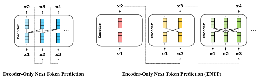
Figure 1: An overview of decoder-only vs. encoder-only Transformers in next token prediction. Decoders use a causal attention, ensuring that each token attends only to the preceding tokens. In contrast, encoders allow all tokens to attend to each other by performing attention computation from scratch for each token prediction.

2 Related Work

Expressive Power of Transformers.

There have been various literature exploring the expressive power of Transformers. From the lens of universal approximation, Yun et al. (2020) showed that any continuous sequence-to-sequence function over a compact set can be approximated arbitrary close by a Transformer (of finite albeit very large size). Other works approach expressiveness from the perspective of computability and complexity such as Pérez et al. (2021) which showed Transformers are Turing complete and Merrill et al. (2022); Merrill & Sabharwal (2024); Li et al. (2024) which use circuit complexity to characterize the languages recognizable by Transformers of fixed depth. Giannou et al. (2023) presents a framework for Transformers as universal computers by placing them in a loop. Communication complexity has also been used to show the impossibility of one-layer Transformers of expressing certain functions e.g. induction head, without the model size being linear in the length of the input (Sanford et al., 2024b; a). However, none of these theories have directly compared the expressive power of encoder and decoder (and specifically of the same fixed model size).

Transformer Architectures for Next Token Prediction.

Transformers have become the de facto backbones for next-token prediction tasks, leading to several variants such as encoder-decoder, causal decoder-only, and prefix decoder-only models. In the encoder-decoder model (Lewis et al., 2019; Chung et al., 2024), similar to the vanilla Transformer (Vaswani et al., 2017), the encoder transforms the input tokens into conditioning features, and the decoder auto-regressively predicts the target tokens by using cross-attention over the encoded representation and causal attention over the output tokens. In contrast, the causal decoder-only model (Brown et al., 2020; Chowdhery et al., 2023) uses only the Transformer decoder and applies causal attention to all tokens to perform next-token prediction, ensuring that each token attends only to previous tokens. The prefix decoder-only model (Raffel et al., 2020; Wu et al., 2021) is similar to the causal decoder-only model but differs in that it applies non-causal attention (i.e., full self-attention) to the input sequence (see Figure 8 for visualizations of the attention patterns in these variants).

With the development of these models, recent studies have investigated the performance of each variant across various tasks. Notably, Wang et al. (2022) examined the zero-shot generalization performance of each model along with various objectives, and Ding et al. (2024) analyzed the performance of causal decoder-only and prefix decoder-only models in in-context learning. However, despite these diverse studies, there is a lack of research on encoder-only models that do not impose the constraint of causal attention for every next token prediction. Therefore, in this work, we analyze the characteristics of encoder-only next-token prediction (ENTP), comparing them with decoder-only models.

3 Preliminaries

Sequence-to-Token Functions and Autoregression.

Given a vocabulary $V$ (which we traditionally think of as some finite set, but could in general be any arbitrary perhaps uncountable set e.g. $\mathbb{R}^{d}$), we can define a sequence over $V$ as $(x_{1},\dots,x_{n})$ where $x_{1},\dots,x_{n}\in V.$ Let $V^{*}=\{(x_{1},\dots,x_{n}):n\in\mathbb{N};x_{i}\in V\}$ be the set of all sequences generated by $V$. Then, we say that $f:V^{*}\to V$ is a sequence-to-token function.

We can view a causal model as a map from an input sequence to an output sequence with the causality constraint that the $i$’th ouput token depends only on the first $i$ input tokens. Mathematically, we enforce this causality contraint by characterizing our causal model, $\mathcal{T}_{f}:V^{*}\to V^{*}$, with some sequence-to-token function $f$ where on input sequence $(x_{1},\dots,x_{n})$ we have that

$$\mathcal{T}_{f}(x_{1},x_{2},\dots,x_{n})\coloneqq(f(x_{1}),f(x_{1},x_{2}),\dots,f(x_{1},x_{2},\dots,x_{n})).$$ (1)

Observe that a sequence-to-token function $f$ can be used auto-regressively to generate tokens from some initial sequence $(x_{1},\dots,x_{n})$ via the following update rule:

$$x_{n+i}\coloneqq f(x_{1},\dots,x_{n+i-1}).$$ (2)

This can also be viewed as a special case of the causal model, where the input sequence is chosen so that

$$\mathcal{T}_{f}(x_{1},x_{2},\dots,x_{n})=(x_{2},x_{3},\dots,x_{n+1}).$$ (3)

Hence, if we are trying to learn a causal or auto-regressive model, it suffices to learn the sequence function that generates it. Thus in this paper, we focus on the type of sequence functions that encoders versus decoders can learn and express.

Encoders and Decoders.

We will use the letters $\mathcal{E}$ and $\mathcal{D}$ respectively to refer to encoders and decoders. In this paper, both models refer to variants of the Transformer architecture introduced in Vaswani et al. (2017), where the only difference lies in the masking used on the attention scores (decoder uses a causal mask while encoder allows full attention, as illustrated in Figure 1). The model size of a Transformer is determined by two parameters:

• $L$: number of Transformer blocks.

• $D$: embedding dimension.

As Transformers are sequence-to-sequence maps, we will use subscript notation where $\mathcal{T}(x_{1},\dots,x_{n})_{i}$ denotes the $i$’th value in the output sequence. We also allow our models the option to use positional embeddings. Tilde-notation i.e. $\widetilde{\mathcal{E}}$ and $\widetilde{\mathcal{D}}$ will denote models that do not use positional embeddings. For token embeddings $x_{1},\dots,x_{n}$ and positional embeddings $p_{1},\dots,p_{n}$:

$$\mathcal{E}(x_{1},\dots,x_{n})\coloneqq\widetilde{\mathcal{E}}(x_{1}+p_{1},\dots,x_{n}+p_{n}).$$

In our experiments, we will use encoder and decoder models that have access to trainable positional embeddings.

Encoder and Decoders as Causal Models.

Given encoder $\mathcal{E}$ and decoder $\mathcal{D},$ we can associate them with sequence-to-token functions as follows:

$$f_{\mathcal{E}}:(x_{1},\dots,x_{n}) \mapsto\mathcal{E}(x_{1},\dots,x_{n})_{n}$$

$$f_{\mathcal{D}}:(x_{1},\dots,x_{n}) \mapsto\mathcal{D}(x_{1},\dots,x_{n})_{n}.$$

We then have $\mathcal{T}_{\mathcal{E}}$ and $\mathcal{T}_{\mathcal{D}}$ as the causal models of $\mathcal{E}$ and $\mathcal{D}$ when used as sequence functions $f_{\mathcal{E}}$ and $f_{\mathcal{D}}$ respectively. Under this characterization, we make two observations. Firstly, we can view $\mathcal{T}_{\mathcal{E}}$ as an explicit and necessary way to introduce causality to the encoder $\mathcal{E}$ since there is nothing implicit to the encoder that forces causality. Secondly, in juxtaposition to the previous statement, the causal model $\mathcal{T}_{\mathcal{D}}$ is exactly equivalent to just using $\mathcal{D}$, that is $\mathcal{T}_{\mathcal{D}}=\mathcal{D}.$ This is because $\mathcal{D}$ enforces causality implicitly via the attention mask (see Section A.2 for formal proof). Therefore the explicit enforcement becomes redundant.

4 Expressive Power of Encoder-only vs. Decoder-only Transformers

Given that we can learn causal functions using either encoders and decoders, the natural question to ask is how the expressive power of each model is related, i.e. can the encoder express more causal functions than a decoder of the same model size? Or perhaps they express the exact same class of causal functions? Towards answering this question, one trivial observation is that there exists causal functions that encoders and decoders are equally well equipped to represent:

Remark 1.

For any $L\geq 1$ and $D\geq 1,$ there exists a decoder $\mathcal{D}$ and encoder $\mathcal{E}$ that each has $L$-layers, embedding dimension $D$ and context window $N,$ and $\mathcal{T}_{\mathcal{D}}(x_{1},x_{2},\dots x_{n})=\mathcal{T}_{\mathcal{E}}(x_{1},x_{2},\dots)$ for all input sequence $(x_{1},x_{2},\dots,x_{n})$ with $x_{1},x_{2},\dots x_{n}\in\mathbb{R}^{D}$.

The above result follows directly from the fact that one-layer decoders and encoders are equivalent (formal proof in Section A.3). Hence, any encoder and decoder that have the same weights in the first layer, and then act as the identity map in the subsequent layers will suffice. Given Remark 1, one may further conjecture that an encoder has strictly larger expressive power than decoders, e.g. given an encoder and decoder model of the same fixed size, the family of causal (but not necessarily auto-regressive) models representable by the encoder model is strictly larger and contains the family of causal functions decoders can represent. This intuitively follows, as by “relaxing” the causal mask to full attention, the embedding of each token in an encoder can still attend to tokens up to and including itself (as in a decoder) while additionally gaining the ability to attend to tokens after it.

However, this is not really the case — there exists causal functions expressible only by encoders, only by decoders, and by both. As intuition, consider some hypothetical task that heavily rely on the inductive bias created by the causal mask, we would expect it to be easy for a decoder to express. To motivate this perspective, we give the following two theorems:

Theorem 1.

For any $L\geq 2$ and $D\geq 1,$ there exists a position-free decoder $\widetilde{\mathcal{D}}$ that has $L$-layers and embedding dimension $D,$ such that for any encoder $\mathcal{E}$, there exists some input sequence $(x_{1},x_{2},\dots)$ with $x_{1},x_{2},\dots\in\mathbb{R}^{D},$ and $\mathcal{T}_{\widetilde{\mathcal{D}}}(x_{1},x_{2},\dots)\neq\mathcal{T}_{\mathcal{E}}(x_{1},x_{2},\dots)$.

Theorem 2.

For any $L\geq 2$ and $D\geq 1,$ there exists a position-free encoder $\widetilde{\mathcal{E}}$ that has $L$-layers and embedding dimension $D,$ such that for any decoder $\mathcal{D}$ with positional embeddings satisfying $p_{1}\neq p_{2}$, there exists some input sequence $(x_{1},x_{2},\dots)$ with $x_{1},x_{2},\dots\in\mathbb{R}^{D},$ and $\mathcal{T}_{\widetilde{\mathcal{E}}}(x_{1},x_{2},\dots)\neq\mathcal{T}_{\mathcal{D}}(x_{1},x_{2},\dots)$.

These theorems are existential in nature. Informally, Theorem 1 says that if we consider causal model defined over the entirety of $\mathbb{R}^{D}$ as its vocabulary, we can find some decoder, for which any encoder will differ from it on some input sequence. Theorem 2 makes a similar (albeit weaker statement) in the other direction; namely the existence of a causal function computable by an encoder, but not by any decoder that uses “non-trivial” positional embeddings (e.g. embeddings for different positions are unique). Detailed proof of both theorems are deferred to Appendix A.

Of course, the setting and assumptions of the above two statements are not necessarily very realistic. For one, they focus on general class of causal models rather than only auto-regressive ones. Furthermore, the results only pertain to exact realization and say nothing about approximation. The assumption of unbounded domain is also not realistic as in practice decoders are trained and used over a finite domain of tokens, each with some fixed embeddings. And specific to Theorem 2, no claim is made about decoders that do not use positional embeddings. But despite the limitations, these theorems give an indication that the expressive power of encoder and decoder model are different — despite the almost identical description modulo the attention mask. Changing the mask on the attention scores causes significant changes to the properties of the model. Thus, in the following sections we propose an auto-regressive tasks and run experiments comparing encoders and decoders that corroborates this view.

5 Time and Space Complexity Comparisons

Inspired by the different computational models of encoder-only and decoder-only Transformers, we characterize the causal sequence functions learnable by encoders and decoders based on their required computational complexity. We give an informal comparison of encoders and decoders in terms of their required time and space complexities — both over the entire sequence and for each additional token. Using the “gap” between the complexity of encoders and decoders, we propose the Triplet-Counting task, which is feasible for an encoder but challenging for a decoder due to its limited computation complexity.

Time Complexity Comparison.

Because an encoder has to compute $O(n^{2})$ attention scores from scratch for each token, it takes $O(n^{2})$ time to generate each token. Thus, it takes $O(n^{3})$ time to generate the entire sequence. We could generate tokens similarly using a decoder. However, due to causality, we can cache the previous keys and values (Kwon et al., 2023), allowing token generation in $O(n)$ time and sequence generation in $O(n^{2})$ time. Given the gap in time complexity between encoders and decoders over an entire sequence ($O(n^{3})$ vs. $O(n^{2})$), this suggests that any causal function that can be expressed by an encoder requiring $\omega(n^{2})$ time cannot be efficiently expressed by a decoder.

Space Complexity Comparison.

Both encoder-only and decoder-decoder use $O(n)$ space complexity to generate an entire sequence. Although the standard implementation of attention uses $O(n^{2})$ space, attention can be implemented using only $O(n)$ space. For details of algorithmic implementations of attention using $O(n)$ memory, refer to Algorithm 3 in the appendix. Thus, we need a more detailed approach to find a difference between the space complexity of the two models.

Towards this end, we classify memory used for the computation over the current token as either precomputed or additional. Precomputed memory stores values from computation over past tokens. Values stored in precomputed memory persist, and are used for computation over current and future tokens, e.g. the keys and values of previous tokens for a decoder. Additional memory stores values that depend on the current token, e.g. keys and values of the current token.

When generating the $n$th token, a decoder uses $O(n)$ precomputed memory to store keys and values of previous tokens and $O(1)$ additional memory to compute results over the current token. An encoder computes everything from scratch for each token, so it uses $O(n)$ additional memory and no precomputed memory. Under this view, there is a space complexity gap between encoder and decoder.

Table 1: Complexity for next token inference.

Complexity	Encoder-only	Decoder-only
Additional Time Complexity	$O(n^{2}DL)$	$O(nDL)$
Precomputed Space Complexity	N/A	$O(nDL)$
Additional Space Complexity	$O(nD)$	$O(D)$

Most of our complexity analysis focuses on Transformers with fixed sizes, so we primarily consider complexity with respect to the sequence length $n$. However, we also account for the embedding dimension $D$ and the number of layers $L$ in Table 1. Both encoder-only and decoder-only Transformers use $O(LD)$ time because the attention operation is performed $O(L)$ times, and computing each query, key, and value vector is $O(D)$. In the case of multi-head attention, we assume $D=hd$, where $h$ is the number of heads and $d$ is the dimension of the query, key, and value vectors. A decoder uses $O(nhdL)=O(nDL)$ precomputed space because it stores $nhL$ query, key, and value $d$-dimensional vectors. Both encoders and decoders use $O(D)$ additional space for current token’s embedding vector — and we specifically note that there is no dependence on $L$ as Transformer do computation sequentially on the layer (i.e. all the additional computation required for layer $\ell$ is done before all the additional computation required for layer $\ell+1$). Thus, we can do the computation over $L$ layers using $O(D)$ space by overwriting computation over previous layers.

5.1 Triplet-Counting Definition and Complexity

Consider the sequence function that maps an input sequence of positive integers $x_{1},x_{2},\dots,x_{n}$ to the number of pairs $x_{i},x_{j}$ where the modulo-$n$ sum of $x_{i},x_{j}$ and $x_{n}$ is equal to $0$. More formally,

$$f_{\text{TC}}(x_{1},x_{2},\dots,x_{n})\coloneqq\Big{|}\big{\{}(i,j)\in[n]^{2}:x_{i}+x_{j}+x_{n}\equiv 0\pmod{n}\big{\}}\Big{|}\pmod{n}.$$ (4)

Now note that there exists algorithms that can compute $f_{\text{TC}}$ on some length-$n$ input sequence $x_{1},x_{2},\dots,x_{n}$ in either $O(n^{2})$ time and $O(1)$ space or in $O(n)$ time and $O(n)$ space. See Algorithm 1 and Algorithm 2 for exact pseudocode implementations. In brief, Algorithm 1 iterates through all $n^{2}$ pairs checking if they meet the modulo-$n$ sum requirement. Algorithm 2 uses the fact that $x_{i}+x_{j}+x_{n}\equiv 0\pmod{n}$ is equivalent to $x_{i}+x_{n}\pmod{n}\equiv-x_{j}\pmod{n}$. In two linear passes, it counts each $-x_{j}\pmod{n}$ and stores each count in a table, then sums the values in the table for each $x_{i}+x_{n}\pmod{n}$. Now, given these two algorithms, we make the following conjecture:

Conjecture 1.

Given an algorithm $\mathcal{A}$ that computes $f_{\text{TC}}(x_{1},x_{2},\dots,x_{n})$, at least one of the following must hold true:

1. $\mathcal{A}$ requires $\Omega(n^{2})$ time with access to $x_{n}$

2. $\mathcal{A}$ requires $\Omega(n)$ space storing values unique to $n$.

This conjecture seems plausible given that both Algorithm 1 and Algorithm 2, which we consider to be optimal, adhere to it. Algorithm 1 uses $O(n^{2})$ time after accessing $x_{n}$ (line 4 of Algorithm 1) and Algorithm 2 requires $O(n)$ memory, where the stored values are a function of $n$ (line 4 of Algorithm 2). Given this conjecture, we can show the following lemma:

Lemma 1.

Given that Conjecture 1 holds and assuming $O(\log n)$ precision, any decoder-only Transformer with fixed embedding dimension $D$ satisfying $\mathcal{D}(x_{1},\dots,x_{m})_{m}=f_{\text{TC}}(x_{1},\dots,x_{m})$ for all sequences of length $m\leq n$ must have $L=\Omega(n)$.

Proof.

Let $\mathcal{D}$ be a decoder with $L$ layers and embedding dimension $D$ satisfying $\mathcal{D}(x_{1},\dots,x_{m})_{m}=f_{\text{TC}}(x_{1},\dots,x_{m})$ for all sequences of length $m\leq n$. We can use $\mathcal{D}$ as an algorithm to compute $f_{\text{TC}}(x_{1},\dots,x_{n})$, by outputting $\mathcal{D}(x_{1},\dots,x_{n})_{n}$ on input $(x_{1},\dots,x_{n}).$ Thus either condition (i) or (ii) of Conjecture 1 must hold when $\mathcal{D}$ computes the output sequence over $(x_{1},\dots,x_{n})$.

Case 1: (i) is true.

In this case $\mathcal{D}$ requires $\Omega(n^{2})$ time with access to $x_{n}$, i.e. $\mathcal{D}$ uses $\Omega(n^{2})$ time for the last token. From Table 1, we know that $\mathcal{D}$ uses $O(nLD)$ time for each token. Thus condition (i) is true only if we have that $nLD=\Omega(n^{2}).$ Since $D$ is fixed, it follows that $L=\Omega(n).$

Case 2: (ii) is true.

In this case, $\mathcal{D}$ requires $\Omega(n)$ space storing values unique to $n$. Because decoders are causal, we have $\mathcal{D}(x_{1},\dots,x_{n})_{i}=f_{\text{TC}}(x_{1},\dots,x_{i})$ for all $i\in[n]$. Then since we assume (ii) is true, computing $\mathcal{D}(x_{1},\dots,x_{n})_{i}$ requires $\Omega(i)$ space for each $i\in[n]$. Furthermore by the uniqueness assumption of (ii), for $i\neq j$, the values stored when computing $f_{\text{TC}}(x_{1},\dots,x_{i})$ are different from the values stored when computing $f_{\text{TC}}(x_{1},\dots,x_{j})$. Since decoders are causal, the space used to compute $\mathcal{D}(x_{1},\dots,x_{n})_{i}$ cannot be overwritten when computing $\mathcal{D}(x_{1},\dots,x_{n})_{j}$, for $j>i$. Hence, when $\mathcal{D}$ computes $f_{\text{TC}}(x_{1},\dots,x_{n})$, it uses $\Omega(i)$ space to compute $f_{\text{TC}}(x_{1},\dots,x_{i})$, for each $i\in[n]$. Thus, $\mathcal{D}$ uses $\Omega\left(\sum_{i\in[n]}i\right)=\Omega(n^{2})$ space to compute $f_{\text{TC}}(x_{1},\dots,x_{n})$. From Table 1, we know that $\mathcal{D}$ uses $O(nLD)$ space for the entire sequence. Then $nLD=\Omega(n^{2})$. Since $D$ is fixed, it follows that $L=\Omega(n).$

Finally, as $L=\Omega(n)$ is a necessary condition for both conditions (i) and (ii), Lemma 1 follows. ∎

Algorithm 1 Algorithm to compute Triplet-Counting in $O(n^{2})$ time and $O(1)$ space

0:  length $n$ sequence of integers $(x_{1},\dots,x_{n})$

1:  $\text{count}\leftarrow 0$

2:  for $i=1,\dots,n$ do

3:      for $j=1,\dots,n$ do

4:           if $(x_{i}+x_{j}+x_{n})\equiv 0\pmod{n}$ then

5:               $\text{count}\leftarrow\text{count}+1$

6:  return  $\text{count}\pmod{n}$

Algorithm 2 Algorithm to compute Triplet-Counting in $O(n)$ time and $O(n)$ space

0:  length $n$ sequence of integers $(x_{1},\dots,x_{n})$

1:  $\text{count}\leftarrow 0$

2:  table $\leftarrow$ zero-indexed length-$n$ array of $0$’s

3:  for $i=1,\dots,n$ do

4:      $k\leftarrow-x_{i}\mod n$

5:      $\text{table}[k]\leftarrow\text{table}[k]+1$

6:  for $i=1,\dots,n$ do

7:      $k\leftarrow(x_{i}+x_{n})\mod n$

8:      $\text{count}\leftarrow\text{count}+\text{table}[k]$

9:  return  $\text{count}\pmod{n}$

Lemma 2.

Assuming $O(\log n)$ precision, there exists an encoder $\mathcal{E}$ with $L=O(1)$ and $D=O(1)$ such that $\mathcal{E}(x_{1},\dots,x_{m})_{m}=f_{\text{TC}}(x_{1},\dots,x_{m})$ for all sequences of length $m\leq n$.

Proof of Lemma 2 is in Section A.6.

Remark 2.

With linear chain-of-thought (generating $O(n)$ tokens before answering), a decoder would be able to perform Triplet-Counting. We provide a RASP (Weiss et al., 2021) program, Algorithm 6, to demonstrate this.

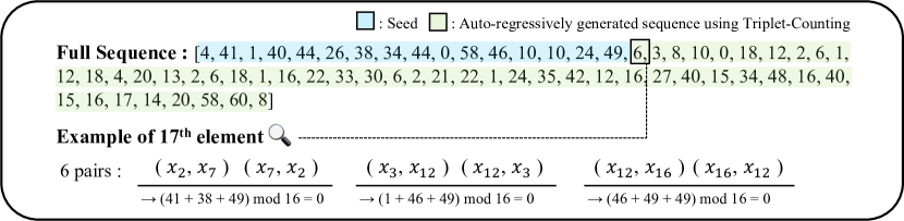
Figure 2: An example of a sequence used in a Triplet-Counting experiment.

5.2 Small-Scale Experiment

We train small decoder-only and encoder-only Transformers on auto-regressive sequences generated from Equation 4.

To generate unique sequences, we start each sequence with a seed containing 16 random integers between 0 and 63. Then we extend the sequence to 64 integers using Equation 4 (see Figure 2). Seeds are generated randomly during training. The seed portion of the sequence was not used to compute the loss during training, so the model was only trained on the deterministic part of the sequence. As shown in Figure 3, the decoder-only Transformers demonstrate some ability to learn patterns related to the distribution of numbers in Triplet-Counting sequences, but they completely fail to learn the task. In contrast, the encoder successfully learns the task with near-perfect accuracy.

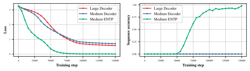
Figure 3: Training loss and sequence accuracy curve for the Triplet-Counting. The ENTP successfully learns to perform the Triplet-Counting task, but the decoder-only models struggle to learn it.

5.3 Triplet-Counting with Large Language Model

Furthermore, we investigate the performance of decoder-only large language models (LLMs) on the Triplet-Counting task. We fine-tune Llama-3 (Dubey et al., 2024) and GPT-4o (Achiam et al., 2023) using sequences of 64 integers, including 16 seeds, as introduced in Section 5.2. To enable the LLMs to leverage their knowledge, we also include the code for Algorithm 1 in the prompt, asking the models to provide the result after executing the code (see Table C.1 for the full prompt). As shown in Figure 4, the LLMs struggle with the Triplet-Counting task, which is consistent with our small-scale experiment. It demonstrates that the suggested characteristics of causal decoder-only models hold true even at large scales. We provide the validation of the prompt design used, as well as details about the LLM fine-tuning, in the Appendix C.1.

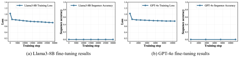
Figure 4: Results of LLM fine-tuning on Triplet-Counting.

Triplet-Counting sequences have very small Kolmogorov complexity, as Algorithm 1 demonstrates with only 6 lines of pseudocode. However, as shown by Lemma 1 and the experiments in Section 5.3, a decoder, no matter how large, cannot efficiently learn the task.

5.4 Triplet-Identification

Motivated by the question of how we need to change the Triplet-Counting task so that it can be learned by a decoder, we examine the Triplet-Identification task.

$$f_{\text{TI}}(x_{1},x_{2},\dots,x_{n})\coloneqq\begin{cases}1&\exists\ (i,j):x_{1}+x_{i}+x_{j}=0\mod 128\\ 0&\text{otherwise}\\ \end{cases}$$ (5)

There are several key differences between $f_{\text{TC}}$ and $f_{\text{TI}}$:

1. $f_{\text{TI}}$ uses a fixed modulus, whereas $f_{\text{TC}}$ employs the sequence length as the modulus. This simplifies the decoder’s task, as the modulus remains constant across all tokens, enabling reuse of intermediate values from previous tokens.

2. $f_{\text{TI}}$ operates on triplets $(x_{1},x_{i},x_{j}$) rather than $(x_{i},x_{j},x_{n}$). By using $x_{1}$ instead of $x_{n}$, it becomes easier for the decoder since $x_{1}$ remains unchanged for different tokens, facilitating the reuse of intermediate values across tokens.

3. $f_{\text{TI}}$ checks for the existence of a condition rather than counting occurrences. Counting is challenging to implement within the attention mechanism without scaling values by the sequence length. Due to the causal mask, scaling value vectors by sequence length is not straightforward.

We provide RASP (Weiss et al., 2021) program, Algorithm 5 that satisfies $\mathcal{D}(x_{1},x_{2},...,x_{n})_{n}=f_{\text{TI}}(x_{1},x_{2},...,x_{n})$ for sequences of any length, assuming $O(\log n)$ precision. We train small Transformers to verify that both decoders and encoders can perform Triplet-Identification, and find that both models can perform Triplet-Identification with high accuracy.

Table 2: Triplet-Identification performance.

Model	Min Loss	Individual Token Accuracy	Full Sequence Accuracy
Medium Decoder (6 layer)	0.0001	99.99%	99.92%
Medium Encoder (6 layer)	0.0016	99.97%	99.50%

6 More Realistic Settings

6.1 Generalization on Addition

We test the sample complexity and length generalization capabilities of decoders and encoders using addition tasks. We use the reversed addition format ($123+456=975$) from Lee et al. (2023). We find that encoders exhibit lower sample complexity compared to decoders, as seen in Figure 6, meaning they require fewer training examples to achieve similar performance. Additionally, encoders demonstrate superior ability to generalize to longer sequences, as shown in Figure 6. We provide more experimental details and results in Section C.3.

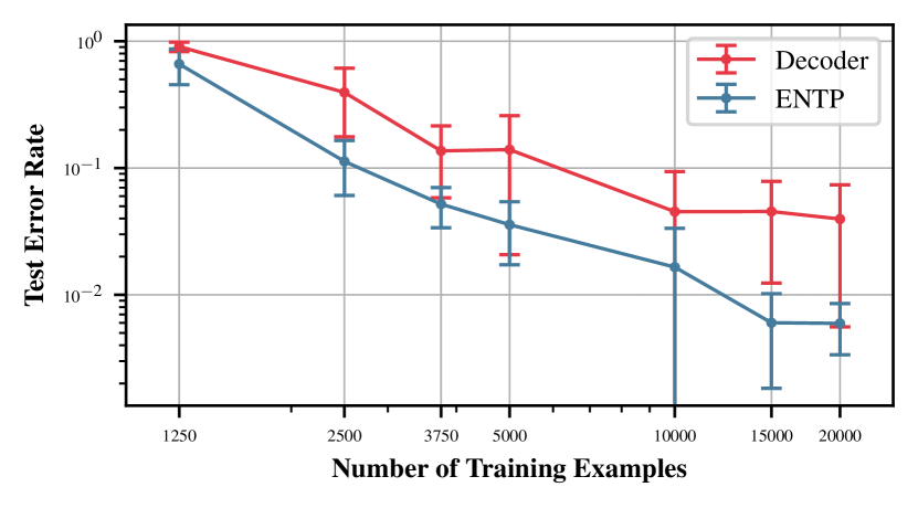
Figure 5: Addition Sample Complexity. The train and test datasets include numbers with up to 3 digits.
 

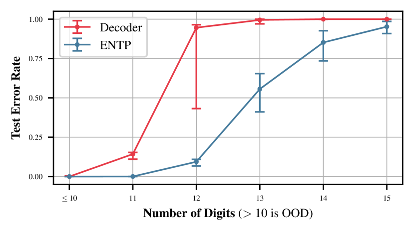
Figure 6: Addition Length Generalization. The train dataset includes numbers with up to 10 digits, and the test dataset has numbers with up to 15 digits.

6.2 In-Context Learning

We consider the problem of learning a function class $\mathcal{F}$ using in-context example (Garg et al., 2022). In this problem, a function $f\in\mathcal{F}$ is sampled from a distribution $\mathcal{D_{F}}$, and a sequence of random inputs is sampled i.i.d. from $\mathcal{D_{X}}$, forming a prompt $P$ : $\left(x_{1},f\left(x_{1}\right),x_{2},f\left(x_{2}\right),\ldots,x_{N},f\left(x_{N}\right)\right)$. The objective is for the model to in-context learn the function $f$ from the prompt $P$ and predict $f(x_{\text{query}})$ for a new input $x_{\text{query}}$. To this end, we train the model $M_{\theta}$, parameterized by $\theta$, by minimizing the expected loss over random sampled prompts as follows:

$$\min_{\theta}\mathbb{E}_{P}\left[\frac{1}{N}\sum_{i=1}^{N-1}\ell\left(M_{\theta}\left(P^{i}\right),f\left({x}_{i+1}\right)\right)\right],$$ (6)

where $\ell(\cdot,\cdot)$ is loss function and $P^{i}$ refers to the partial prompt containing $i$ in-context examples with $(i+1)^{th}$ input (i.e., $\left({x}_{1},f\left({x}_{1}\right),\ldots,{x}_{i},f\left({x}_{i}\right),{x}_{i+1}\right)$).

In this work, we examine four types of function classes: linear function, sparse linear function, two-layer neural network and decision tree. For all function classes, we sample $x_{i}$ from a Gaussian distribution $N\left(0,\mathbf{I}_{d}\right)$ where $d$ represents the dimension of $x_{i}$, and utilize the squared error as loss function. Detailed descriptions for each function class are provided in Appendix C.2.

We provide the in-context-learning results according to the number of in-context examples for each function class in Figure 7. The encoder-only models demonstrate better performance compared to the decoder-only models in linear regression and sparse linear regression, while exhibiting competitive performance in two-layer NN regression and decision tree.

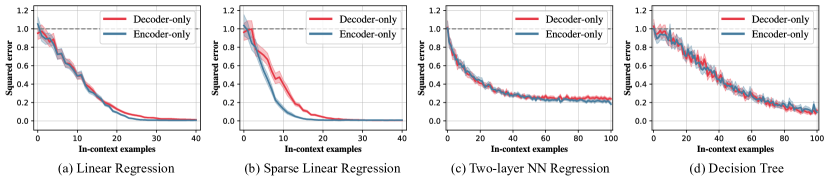
Figure 7: Results of in-context learning experiment. The encoder-only models demonstrate superior or competitive performance across all function classes compared to the decoder-only models.

6.3 OpenWebText

We train Transformers on the OpenWebText dataset (Gokaslan et al., 2019), an open-source replication of the WebText dataset used to train GPT-2 (Radford et al., 2019), with the next-token prediction objective. We use medium models, described in Table 5. As shown in Table 3, encoder-only Transformer slightly outperforms decoder-only Transformer.

Table 3: Minimum values of training and validation loss, as well as perplexity, for decoder-only and encoder-only Transformers on the OpenWebText dataset.

Model	Train Loss	Validation Loss	Train Perplexity	Validation Perplexity
Decoder-only	4.694	4.705	109.3	110.5
Encoder-only	4.643	4.650	103.9	104.6

7 Conclusion and Future Work

In this work, we present theoretical and novel experimental results suggesting that, assuming compute is unlimited, decoder-only Transformers are not the ideal model for sequence modeling. We show that ENTP is more expressive without compromising generalization. Using Theorem 1 and 2, we find that the classes of functions encoder-only and decoder-only Transformers can exactly learn are different. We introduce the Triplet-Counting task and demonstrate, both theoretically (assuming Conjecture 1) and experimentally, that while encoders can perform this task easily, decoders cannot. We also find that encoders outperform decoders on a variety of auto-regressive tasks, including length generalization and in-context learning. However, the expressivity gained by removing the causal mask comes at the expense of efficiency.

Future Work.

Several open avenues for further research remain in ENTP theory, such as proving Lemma 1 without relying on Conjecture 1 (or providing a counterexample) and generalizing Triplet-Counting to a broader class of tasks where encoders perform well but decoders do not. Further investigation into length generalization across tasks beyond addition is valuable to confirm the findings of this paper. Another natural extension of our work would be to explore whether we can further enhance expressivity past ENTP. In a more practical direction, as both training and inference with ENTP are compute-intensive, future work may focus on reducing computational costs. For instance, could we first train a decoder and then efficiently convert it to ENTP? Is it possible to combine decoders with ENTP? More broadly, are there better methods for efficiently training ENTP models?

Appendix A Notation and Deferred Proofs

A.1 Notation

• $\mathcal{E}$, $\mathcal{D}$: Encoder/Decoder with positional embeddings.

• $\widetilde{\mathcal{E}}$, $\widetilde{\mathcal{D}}$: Encoder/Decoder without positional embeddings (with same model weights as $\mathcal{E}$, $\mathcal{D}$) (which we call position free).

• $L$: number of Transformer blocks.

• $D$: embedding dimension.

• $p_{i}$: The $i$’th positional embedding where $p_{i}\in\mathbb{R}^{D}$.

• $\mathbf{W}_{Q/K/V}^{i}$: The weight matrix of the Query, Key and Value respectively of the $i$’th attention block.

• $\mathbf{I}$: The identity matrix.

• $\mathbf{0}$: The zero matrix.

• $(x_{1},x_{2},x_{3},\dots)$: A sequence of values/tokens.

• $\mathcal{T}_{\mathcal{E}}(x_{1},x_{2},x_{3},\dots)\coloneqq(\mathcal{E}(x_{1})_{1},\mathcal{E}(x_{1},x_{2})_{2},\mathcal{E}(x_{1},x_{2},x_{3})_{3},\dots)$.

For convention, we will use bold capital letters $\mathbf{X}$ to denote matrices, and unbold lowercase letters $x$ to denote vectors.

For theorem 1 and theorem 2, our model of Transformers will use single-head attention and assume the dimension of the Query and Key are equal to the embedding dimension $D$. We also omit layer normalization and scaling of attention scores by $1/\sqrt{D}.$

A.2 $\mathcal{T}_{\mathcal{D}}=\mathcal{D}$

Proof.

The main observation is that the the MLP layers of a decoder are element-wise, and the attention layers of a decoder are causal (i.e. the contextual embedding of the $i$’th token is computed only using the tokens $j\leq i$). We thus have that

$$\mathcal{D}(x_{1},\dots,x_{i},\dots,x_{n})_{i}=\mathcal{D}(x_{1},\dots,x_{i})_{i}$$

for any $i\in[n].$ As a result,

$$\mathcal{D}(x_{1},\dots,x_{i},\dots,x_{n})_{i} =\mathcal{D}(x_{1},\dots,x_{i})_{i}$$

$$=f_{\mathcal{D}}(x_{1},\dots,x_{i})$$

$$=\mathcal{T}_{\mathcal{D}}(x_{1},\dots,x_{i},\dots,x_{n})_{i},$$

for all $i\in[n],$ i.e. $\mathcal{D}(x_{1},\dots,x_{n})=\mathcal{T}_{\mathcal{D}}(x_{1},\dots,x_{n}).$ ∎

A.3 One-layer Encoder and Decoder are Equivalent

Proof.

Let $\mathcal{D}$ and $\mathcal{E}$ have the same parameters. Then the query key, and value vectors for the attention layer (denoted $q_{i},k_{i},v_{i}$ for each $x_{i}$ respectively) will be the same for both models.

For one-layer decoder: $\mathcal{D}(x_{1},...,x_{n})_{i}=\operatorname{MLP}\left(\sum_{j=1}^{i}\operatorname{Softmax}(q_{i},k_{j})v_{j}\right)$.

For one-layer encoder: $\mathcal{E}(x_{1},...,x_{n})_{i}=\operatorname{MLP}\left(\sum_{j=1}^{n}\operatorname{Softmax}(q_{i},k_{j})v_{j}\right)$.

If $i=n$, then $\mathcal{D}(x_{1},...,x_{n})_{i}=\mathcal{E}(x_{1},...,x_{n})_{i}$. Thus, $\mathcal{T}_{\mathcal{D}}(x_{1},x_{2},\dots,x_{n})=\mathcal{T}_{\mathcal{E}}(x_{1},x_{2},\dots,x_{n})$. ∎

A.4 Proof of theorem 1

Proof.

We first provide a construction for $\widetilde{\mathcal{D}}.$ For the attention-block of the first two layers, we use the same weight matrices. Namely, we set $\mathbf{W}^{1}_{K}=\mathbf{W}^{2}_{K}=\mathbf{W}^{1}_{Q}=\mathbf{W}^{2}_{Q}=\mathbf{0}$ and $\mathbf{W}^{1}_{V}=\mathbf{W}^{2}_{V}=\mathbf{I}$. For every other attention block, we set them to the constant zero function by setting $\mathbf{W}^{i}_{V}=\mathbf{0}$ for $i\geq 3$. We similarly set the weights and biases of every MLP block to zero. Thus, in essence $\widetilde{\mathcal{D}}$ is just two duplicate attention blocks stacked on top of each other with a skip connection after each attention block.

Now consider three arbitrary vectors $x_{1},x_{2},x_{3}\in\mathbb{R}^{D}$ and its corresponding sequence $(x_{1},x_{2},x_{3})$. Let us first compute the output of $\widetilde{\mathcal{D}}$ on $(x_{1},x_{2},x_{3})$. The first attention block and skip connection will map the input sequence to the sequence

$$\left(2x_{1},x_{2}+\frac{x_{1}+x_{2}}{2},x_{3}+\frac{x_{1}+x_{2}+x_{3}}{3}\right).$$

The second attention block and skip connection will then map to the following:

$$\left(4x_{1},\frac{7x_{1}+9x_{2}}{4},\frac{23x_{1}+17x_{2}+32x_{3}}{18}\right).$$

Our first observation from this mapping is that there clearly exists $\tilde{x}_{1},\tilde{x}_{2},\tilde{x}_{3}\in\mathbb{R}^{D}$ such that $\widetilde{\mathcal{D}}(\tilde{x}_{1},\tilde{x}_{2},\tilde{x}_{3})_{3}\neq\widetilde{\mathcal{D}}(\tilde{x}_{2},\tilde{x}_{1},\tilde{x}_{3})_{3}.$ Our second observation is that

$$4x_{1}=\frac{7x_{1}+9x_{2}}{4}\quad\Longleftrightarrow\quad x_{1}=x_{2},$$

which follows from simplifying the left hand equation.

Now, let us for sake of contradiction assume the existence of some encoder $\mathcal{E}$ such that $\mathcal{T}_{\mathcal{E}}$ exactly replicates $\widetilde{\mathcal{D}}$ on every input sequence. We first claim that the first two positional embeddings $p_{1},p_{2}$ of $\mathcal{E}$ must differ. This follows by our first observation and thus the requirement that $\mathcal{E}(\tilde{x}_{1},\tilde{x}_{2},\tilde{x}_{3})_{3}\neq\mathcal{E}(\tilde{x}_{2},\tilde{x}_{1},\tilde{x}_{3})_{3}$ — which can only happen if $p_{1}\neq p_{2}$ due to the permutation invariance of encoders when there are no positional embeddings. Now as $p_{1}\neq p_{2}$, there exists vectors $y_{1},y_{2},c\in\mathbb{R}^{D}$ such that $y_{1}\neq y_{2}$ and $y_{1}+p_{1}=y_{2}+p_{2}=c$. It follows immediately that

$$\mathcal{E}(y_{1})_{1} =\widetilde{\mathcal{E}}(y_{1}+p_{1})_{1}$$

$$=\widetilde{\mathcal{E}}(c)_{1}$$

$$=\widetilde{\mathcal{E}}(c,c)_{2}$$

$$=\widetilde{\mathcal{E}}(y_{1}+p_{1},y_{2}+p_{2})_{2}$$

$$=\mathcal{E}(y_{1},y_{2})_{2}.$$

But since $y_{1}\neq y_{2}$, by the second observation we made, it must be that $\widetilde{\mathcal{D}}(y_{1})_{1}\neq\widetilde{\mathcal{D}}(y_{1},y_{2})_{2}$. Since we assumed that $\mathcal{T}_{\mathcal{E}}$ exactly replicates $\widetilde{\mathcal{D}}$ on every input sequence, it thus follows that $\mathcal{E}(y_{1})_{1}\neq\mathcal{E}(y_{1},y_{2})_{2}$ — a contradiction. Hence, no such encoder $\mathcal{E}$ exists, which directly implies that we can always find some sequence $(x_{1},x_{2},\dots)$ where $\widetilde{\mathcal{D}}(x_{1},x_{2},\dots)\neq\mathcal{T}_{\mathcal{E}}(x_{1},x_{2},\dots)$. ∎

A.5 Proof of theorem 2

Proof.

We first provide a construction for $\widetilde{\mathcal{E}}.$ For the attention-block of the first two layers, we use the same weight matrices. Namely, we set $\mathbf{W}^{1}_{K}=\mathbf{W}^{2}_{K}=\mathbf{W}^{1}_{Q}=\mathbf{W}^{2}_{Q}=\mathbf{W}^{1}_{V}=\mathbf{W}^{2}_{V}=\mathbf{I}$. For every other attention block, we set them to the constant zero function by setting $\mathbf{W}^{i}_{V}=\mathbf{0}$ for $i\geq 3$. We similarly set the weights and biases of every MLP block to zero. Thus, in essence $\widetilde{\mathcal{E}}$ is just two duplicate attention blocks stacked on top of each other with a skip connection after each attention block.

Now consider two arbitrary vectors $x_{1},x_{2}\in\mathbb{R}^{D}$ and its corresponding sequence $(x_{1},x_{2})$. A brief inspection will reveal that

$$\mathcal{T}_{\widetilde{\mathcal{E}}}(x_{1},x_{2})=(4x_{1},\alpha x_{1}+\beta x_{2}),$$ (7)

where $\alpha,\beta>0.$

Next, we assume the existence of some $\mathcal{D}$ where $p_{1}\neq p_{2}$ and exactly replicates $\widetilde{\mathcal{E}}.$ We fix $x_{1}=0$ and let $x_{2}=p_{1}-p_{2}.$ Observe that $x_{2}\neq 0$ as $p_{1}\neq p_{2}$. It follows that there is some constant vector $c\in\mathbb{R}^{D}$ where

$$\mathcal{D}(x_{1},x_{2}) =\widetilde{\mathcal{D}}(x_{1}+p_{1},x_{2}+p_{2})$$

$$=\widetilde{\mathcal{D}}(p_{1},p_{1})$$

$$=(c,c).$$

Now from equation 7, we have that $\mathcal{T}_{\widetilde{\mathcal{E}}}(x_{1},x_{2})=(0,\beta x_{2})$ for some $\beta>0.$ As $x_{2}\neq 0$, it follows that $\beta x_{2}\neq 0$ and hence $(0,\beta x_{2})$ is not a constant sequence — contradicting the output of the decoder. Hence, no $\mathcal{D}$ where $p_{1}\neq p_{2}$ can exactly replicates $\widetilde{\mathcal{E}}.$ ∎

A.6 Proof of lemma 2

Proof.

Lemma 2 follows from Algorithm 4. From Weiss et al. (2021), a RASP program can be compiled to a Transformer, with a fixed number of Transformer-layers and attention heads. However, it assumes that the MLPs can perform any element-wise operation. Thus, it suffices to show that each MLP needs $O(1)$ layers with respect to sequence length $n$.

We first observe that the largest internal value possible within Algorithm 4 is $n^{2}$, so there are $n^{2}+1$ distinct internal values including 0. Using $\lfloor 2\log_{2}n\rfloor+1$ bits, we can represent all of these values as unsigned integers. Using floating-point numbers we would also need $\Theta(\log n)$ bits.

All linear element-wise operations in Algorithm 4 can be implemented trivially, since an MLP can perform arbitrary linear transformations. Therefore, we focus on the only nonlinear element-wise function $g:\mathbb{[}2n-1]\times[n]\rightarrow[n-1]$:

$$g(a,b)=\begin{cases}a,&a<b\\ a-b&a\geq b.\end{cases}$$

Using a constant number of linear operations and $\operatorname{ReLU}$ functions, $g$ can be constructed as follows:

$$g(a,b)=\operatorname{ReLU}(a-M\operatorname{ReLU}(a-b+\epsilon))+\operatorname{ReLU}(a-b),$$

where $0<\epsilon<1$ and $M\geq\frac{2n}{\epsilon}$.

Because $g$ can be implemented using a constant number of linear operations and $\operatorname{ReLU}$ functions, it can be implemented by an MLP with $\operatorname{ReLU}$ activation functions and $O(1)$ depth.

Because of skip-connections, we can concatenate MLPs by zeroing out attention. Then we can create any MLP of $O(1)$ depth.

Thus, it is possible to construct an encoder $\mathcal{E}$ with $L=O(1)$ and $D=O(1)$ such that $\mathcal{E}(x_{1},\dots,x_{m})_{m}=f_{\text{TC}}(x_{1},\dots,x_{m})$ for all sequences of length $m\leq n$. ∎

Appendix B Attention patterns of different Transformer architectures

In Figure 8, we provide the visualization of attention patterns of encoder-only, decoder-only, prefix decoder-only, and encoder-only models.

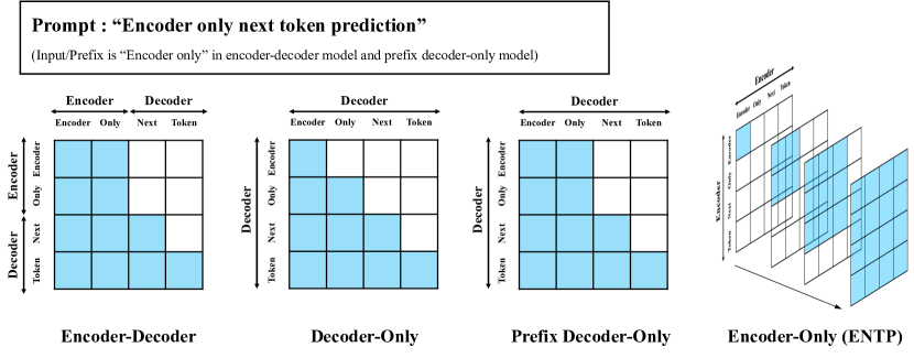
Figure 8: Attention patterns of different Transformer architectures in next token prediction. Encoder-decoder and prefix decoder-only models first perform full attention on the input (prefix), and then use causal attention to predict subsequent tokens. In contrast, decoder-only models apply causal attention to all tokens, without distinguishing between input and output. Encoder-only models also do not separate input and output, but they recalculate attention from scratch for each token prediction, performing full attention on all tokens.

Appendix C Experiment Details

In all experiments, we train encoders in the same manner as decoders, processing entire sequences in each batch with a single gradient optimization step. Although this approach does not offer the same efficiency benefits for encoders as it does for decoders, we adopt it to maintain consistency between the training processes of both models.

C.1 Triplet-counting with LLM

In the main paper, we fine-tuned two LLMs for Triplet-Counting: Llama3-8B (Dubey et al., 2024) and GPT-4o (Achiam et al., 2023). Here, we provide the details about the fine-tuning of each model. For GPT-4o, we used the official API, setting the batch size to 4 and the learning rate multiplier to 10. For Llama3-8B, we employed LoRA fine-tuning Hu et al. (2022) with a batch size of 16 and a learning rate of $1.4\times 10^{-4}$. Regarding prompt design, we included the algorithm code in the prompt so that the LLMs could leverage its knowledge of natural language (see Table C.1). We note that the loss was applied only to the answer part of the prompt.

Additionally, we verify the validity of the prompt design used for LLM fine-tuning. To this end, we modify the task from Triplet-Counting to pair counting and fine-tune the Llama3-8B using prompts that include algorithmic code, as in the main experiment. As shown in Figure 9, the model successfully learns pair counting with the proposed prompt design, achieving high sequence accuracy. This demonstrates that the model’s difficulty in learning Triplet-Counting is due to the characteristics of causal decoder-only architecture, rather than an issue with the training strategy, such as the prompt design.

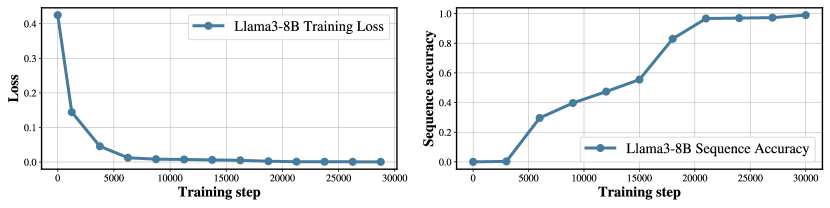
Figure 9: Results of LLM fine-tuning on pair counting. The Llama3-8B successfully learns pair counting when using the same prompt format as Triplet-Counting. This demonstrates that the reason LLMs struggle with Triplet-Counting is not due to the complexity of the prompt, but rather the characteristics of the decoder-only model.

Table 4: Example of prompt used for LLM experiments. We include the code for the algorithm in the prompt to leverage the knowledge of the LLMs.

C.2 In-context Learning

As introduced in the main paper, four types of function classes are considered in the in-context learning experiment (Garg et al., 2022): linear function, sparse linear function, two-layer neural network, and decision tree. For all function classes, the input $x_{i}$ is drawn from a Gaussian distribution $N\left(0,\mathbf{I}_{d}\right)$ where $d$ represents the dimension of $x_{i}$. We provide detailed descriptions of each function class below.

Linear function.

We consider the class of linear functions $\mathcal{F}=\left\{f\mid f({x})={w}^{\top}{x},{w}\in\mathbb{R}^{d}\right\}$ where $w$ is drawn from a Gaussian distribution $N\left(0,\mathbf{I}_{d}\right)$. Following previous work (Garg et al., 2022), we set $d=20$ and the number of data points $N$ to 40.

Sparse linear function.

We also consider a sparse linear function, which is similar to a linear function setup. The difference is that after drawing $w$ from $N\left(0,\mathbf{I}_{d}\right)$, only $k$ randomly selected coordinates are kept, while the remaining ones are set to zero. Following previous work (Garg et al., 2022), we set $k=3$.

Two-layer neural network

We examine the class of two-layer ReLU neural networks $\mathcal{F}=\left\{f\mid f(x)=\mathbf{W}_{(2)}\sigma\left(\mathbf{W}_{(1)}x\right),\mathbf{W}_{(2)}\in\mathbb{R}^{1\times h},\mathbf{W}_{(1)}\in\mathbb{R}^{h\times d}\right\}$ where $\sigma(\cdot)=\max(0,\cdot)$ (i.e., ReLU function). We set $h=100$, $d=20$, and the number of data point $N$ to 100.

Decision tree

We consider the class of decision trees represented by full-binary trees of fixed height. In these trees, the leaf node values are drawn from $N\left(0,1\right)$, and the non-leaf nodes are sampled from random integers between 0 and $d$, indicating an index of the input $x$. At each non-leaf node, if the value of the input at the specified index is positive, we move to the right; otherwise, we move to the left. Given an input, we start at the root node and repeat this process until reaching a leaf node. The value of the leaf node becomes the output of the function.

C.3 Addition

3dhdWe test the sample complexity of encoder-only and decoder-only Transformers using addition tasks, with up to 3-digit numbers. We sample the dataset of all possible 3-digit addition examples using a method similar to the method described in Lee et al. (2023). We start with all 1,000,000 3-digit, 2-digit, and 1-digit addition examples. Then we randomly remove 90% of the 3-digit addition examples, adjusting the ratio of 3-digit to 2-digit examples from around 100:1 to around 10:1. Next we split the data into training, testing, and validation splits, stratified by the number of digits and carries in each addition example. All 1-digit addition examples were put into the training split. Since our models tend to over fit the training dataset, we save the model with the lowest loss on a validation dataset. We test decoder-only and encoder-only Transformers on plain and reversed addition tasks, using between 1.25k to 20k training examples. All sample complexity tests are run with at least 5 different seeds. We test small models, described in Table 5.

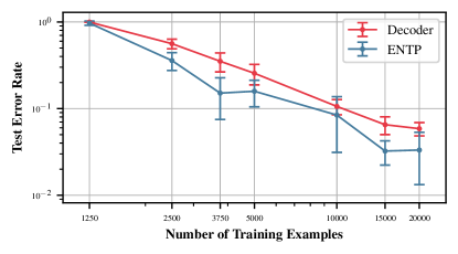
Figure 10: Addition Sample Complexity. The train and test datasets include numbers with up to 3 digits. The dataset uses the plain addition format ($123+456=579$), unlike the results in Figure 6.

We train Transformers to add larger numbers and evaluate their ability to perform length generalization. Training is performed on numbers with up to 10 digits, while testing extends to numbers with up to 15 digits. Each model is trained on 100,000 examples using the reversed addition format (Lee et al., 2023). The numbers are sampled to ensure equal probability for each length, without duplicates. Consequently, in larger datasets, there are fewer 1-digit addition examples compared to 10-digit ones, as the total number of possible 1-digit examples is smaller. All length generalization tests are run with 3 different seeds. We test Small-Deep models described in Table 5.

C.4 Model Sizes

In Table 5, we provide the configurations of the Transformer architectures used in the experiments from the main paper.

Table 5: Model specifications.

Name	Number of Layers	Number of Heads	Embedding Dimension
Small	3	3	192
Medium	6	6	384
Large	12	12	768
Small-Deep	8	2	128

Appendix D Implementation of Attention Using $O(n)$ Memory

Algorithm 3 Implementation of Attention Using $O(n)$ Memory

0:  $q\in\mathbb{R}^{n\times d}$, $k\in\mathbb{R}^{n\times d}$, $v\in\mathbb{R}^{n\times D}$

1:  $y\leftarrow\mathbf{0}^{n\times D}$

2:  for $i=1,\dots,n$ do

3:      $a\leftarrow 0^{D}$

4:      $b\leftarrow 0$

5:      for $j=1,\dots,n$ do

6:           $c\leftarrow\exp(q_{i}^{T}k_{j})$

7:           $a\leftarrow a+cv_{j}$

8:           $b\leftarrow b+c$

9:      $y_{i}\leftarrow\frac{a}{b}$

10:  return  $y$

Appendix E RASP Algorithms

In Algorithm 4, 5, and 6, we provide the Python RASP implementation (Zhou et al., 2024) for Triplet-Counting, Triplet-Identification, and Triplet-Counting with COT.

Algorithm 4 Triplet-Counting RASP Encoder Implementation

⬇

def g(a, b):

return a if a < b else a - b

def count_triplets(x):

idxs = indices(x)

# set n[i] = len(x) and last_x[i] = x[-1] for all i (only possible with encoder)

n = sel_width(select(k=x, q=x, pred=true))

last_x = kqv(k=idxs, q=n - 1, v=x, pred=equals, reduction="mean")

# g(a, b) is equivalent a % b if 0 <= a < 2 * b

y = seq_map(n - x, n, g) # y[i] = -x[i] % n

z = seq_map(x + last_x, n, g) # z[i] = (x[i] + x[-1]) % n

# conut the number of (i, j) such that y[i] == z[j]

# c = sum(A), where A[i, j] = 1 if y[i] == z[j] else 0

c = kqv(

k=full(x, 1),

q=full(x, 1),

v=sel_width(select(k=z, q=y, pred=equals)) * n, # sum(v) = mean(v * n)

pred=equals,

reduction="mean",

)

# conpute count % n

c -= idxs * n

# because count <= n^2, there exists i such that c[i] = count % n or c[i] = n

# the case c[i] = n is handled by the default value (0) when no keys are selected

return kqv(k=c, q=n, v=c, pred=lambda a, b: 0 <= a and a < b, reduction="mean")

Algorithm 5 Triplet-Identification RASP Decoder Implementation

⬇

def has_triplet(x):

idxs = indices(x)

first_x = kqv(k=idxs, q=full(x, 0), v=x, pred=equals, reduction="mean", causal=True)

# use bitmask to compute mod

y = -x & 127 # y[i] = -x[i] % 128

z = (first_x + x) & 127 # z[i] = (x[0] + x[i]) % 128

# max_count[-1] > 0 if there exists (i, j) such that y[i] == z[j]

max_count = kqv(

k=full(x, 1),

q=full(x, 1),

v=sel_width(select(k=y, q=z, pred=equals)),

pred=equals,

reduction="max",

)

return tok_map(max_count, lambda a: min(a, 1)) # return 0 or 1

Algorithm 6 Triplet-Counting RASP Decoder COT Implementation

⬇

def count_triplets(x):

idxs = indices(x)

n = kqv(k=x, q=full(x, EOS), v=idxs, pred=equals, reduction="min", causal=True)

n = tok_map(n, lambda a: a if a else -2)

last_x = kqv(k=idxs, q=n - 1, v=x, pred=equals, reduction="mean")

seq_len = kqv(k=x, q=x, v=idxs, pred=true, reduction="max", causal=True)

i = seq_len - n

j = seq_len - 2 * n

xi = kqv(k=idxs, q=i, v=x, pred=equals, reduction="max", causal=True)

xj = kqv(k=idxs, q=j, v=x, pred=equals, reduction="max", causal=True)

y = (n - xi) % n + 1

z = (last_x + xj) % n + 1

y_mask_write = (n <= idxs) & (idxs < 2 * n)

z_mask_write = (2 * n <= idxs) & (idxs < 3 * n)

y_mask_read = (n < idxs) & (idxs <= 2 * n)

z_mask_read = (2 * n < idxs) & (idxs <= 3 * n)

z_count = sel_width(

select(

k=x * y_mask_read,

q=z,

pred=lambda a, b: a == b and a != 0,

causal=True,

)

)

count = kqv(

k=z_mask_read,

q=z_mask_read,

v=n * x * z_mask_read,

pred=lambda a, b: a & b,

reduction="mean",

causal=True,

)

ans = count % n

ans_mask_write = idxs == 3 * n

eos_mask_write = idxs > 3 * n

return (

y * y_mask_write

+ z_count * z_mask_write

+ ans * ans_mask_write

+ EOS * eos_mask_write

)

References

- Achiam et al. (2023) Josh Achiam, Steven Adler, Sandhini Agarwal, Lama Ahmad, Ilge Akkaya, Florencia Leoni Aleman, Diogo Almeida, Janko Altenschmidt, Sam Altman, Shyamal Anadkat, et al. Gpt-4 technical report. arXiv preprint arXiv:2303.08774, 2023.
- Brown et al. (2020) Tom Brown, Benjamin Mann, Nick Ryder, Melanie Subbiah, Jared D Kaplan, Prafulla Dhariwal, Arvind Neelakantan, Pranav Shyam, Girish Sastry, Amanda Askell, Sandhini Agarwal, Ariel Herbert-Voss, Gretchen Krueger, Tom Henighan, Rewon Child, Aditya Ramesh, Daniel Ziegler, Jeffrey Wu, Clemens Winter, Chris Hesse, Mark Chen, Eric Sigler, Mateusz Litwin, Scott Gray, Benjamin Chess, Jack Clark, Christopher Berner, Sam McCandlish, Alec Radford, Ilya Sutskever, and Dario Amodei. Language models are few-shot learners. In H. Larochelle, M. Ranzato, R. Hadsell, M.F. Balcan, and H. Lin (eds.), Advances in Neural Information Processing Systems, volume 33, pp. 1877–1901. Curran Associates, Inc., 2020.
- Chowdhery et al. (2023) Aakanksha Chowdhery, Sharan Narang, Jacob Devlin, Maarten Bosma, Gaurav Mishra, Adam Roberts, Paul Barham, Hyung Won Chung, Charles Sutton, Sebastian Gehrmann, et al. Palm: Scaling language modeling with pathways. Journal of Machine Learning Research, 24(240):1–113, 2023.
- Chung et al. (2024) Hyung Won Chung, Le Hou, Shayne Longpre, Barret Zoph, Yi Tay, William Fedus, Yunxuan Li, Xuezhi Wang, Mostafa Dehghani, Siddhartha Brahma, et al. Scaling instruction-finetuned language models. Journal of Machine Learning Research, 25(70):1–53, 2024.
- Ding et al. (2024) Nan Ding, Tomer Levinboim, Jialin Wu, Sebastian Goodman, and Radu Soricut. CausalLM is not optimal for in-context learning. In The Twelfth International Conference on Learning Representations, 2024.
- Dubey et al. (2024) Abhimanyu Dubey, Abhinav Jauhri, Abhinav Pandey, Abhishek Kadian, Ahmad Al-Dahle, Aiesha Letman, Akhil Mathur, Alan Schelten, Amy Yang, Angela Fan, et al. The llama 3 herd of models. arXiv preprint arXiv:2407.21783, 2024.
- Garg et al. (2022) Shivam Garg, Dimitris Tsipras, Percy Liang, and Gregory Valiant. What can transformers learn in-context? a case study of simple function classes. In Alice H. Oh, Alekh Agarwal, Danielle Belgrave, and Kyunghyun Cho (eds.), Advances in Neural Information Processing Systems, 2022.
- Giannou et al. (2023) Angeliki Giannou, Shashank Rajput, Jy-Yong Sohn, Kangwook Lee, Jason D. Lee, and Dimitris Papailiopoulos. Looped transformers as programmable computers. In Andreas Krause, Emma Brunskill, Kyunghyun Cho, Barbara Engelhardt, Sivan Sabato, and Jonathan Scarlett (eds.), Proceedings of the 40th International Conference on Machine Learning, volume 202 of Proceedings of Machine Learning Research, pp. 11398–11442. PMLR, 23–29 Jul 2023. URL https://proceedings.mlr.press/v202/giannou23a.html.
- Gokaslan et al. (2019) Aaron Gokaslan, Vanya Cohen, Ellie Pavlick, and Stefanie Tellex. Openwebtext corpus. http://Skylion007.github.io/OpenWebTextCorpus, 2019.
- Hu et al. (2022) Edward J Hu, yelong shen, Phillip Wallis, Zeyuan Allen-Zhu, Yuanzhi Li, Shean Wang, Lu Wang, and Weizhu Chen. LoRA: Low-rank adaptation of large language models. In International Conference on Learning Representations, 2022.
- Kwon et al. (2023) Woosuk Kwon, Zhuohan Li, Siyuan Zhuang, Ying Sheng, Lianmin Zheng, Cody Hao Yu, Joseph Gonzalez, Hao Zhang, and Ion Stoica. Efficient memory management for large language model serving with pagedattention. In Proceedings of the 29th Symposium on Operating Systems Principles, pp. 611–626, 2023.
- Lee et al. (2023) Nayoung Lee, Kartik Sreenivasan, Jason D Lee, Kangwook Lee, and Dimitris Papailiopoulos. Teaching arithmetic to small transformers. In The Twelfth International Conference on Learning Representations, 2023.
- Lewis et al. (2019) Mike Lewis, Yinhan Liu, Naman Goyal, Marjan Ghazvininejad, Abdel rahman Mohamed, Omer Levy, Veselin Stoyanov, and Luke Zettlemoyer. Bart: Denoising sequence-to-sequence pre-training for natural language generation, translation, and comprehension. In Annual Meeting of the Association for Computational Linguistics, 2019.
- Li et al. (2024) Zhiyuan Li, Hong Liu, Denny Zhou, and Tengyu Ma. Chain of thought empowers transformers to solve inherently serial problems. arXiv preprint arXiv:2402.12875, 2024.
- Merrill & Sabharwal (2024) William Merrill and Ashish Sabharwal. A logic for expressing log-precision transformers. Advances in Neural Information Processing Systems, 36, 2024.
- Merrill et al. (2022) William Merrill, Ashish Sabharwal, and Noah A Smith. Saturated transformers are constant-depth threshold circuits. Transactions of the Association for Computational Linguistics, 10:843–856, 2022.
- Pérez et al. (2021) Jorge Pérez, Pablo Barceló, and Javier Marinkovic. Attention is turing-complete. Journal of Machine Learning Research, 22(75):1–35, 2021.
- Radford et al. (2019) Alec Radford, Jeff Wu, Rewon Child, David Luan, Dario Amodei, and Ilya Sutskever. Language models are unsupervised multitask learners. 2019. URL https://api.semanticscholar.org/CorpusID:160025533.
- Raffel et al. (2020) Colin Raffel, Noam Shazeer, Adam Roberts, Katherine Lee, Sharan Narang, Michael Matena, Yanqi Zhou, Wei Li, and Peter J Liu. Exploring the limits of transfer learning with a unified text-to-text transformer. Journal of machine learning research, 21(140):1–67, 2020.
- Sanford et al. (2024a) Clayton Sanford, Daniel Hsu, and Matus Telgarsky. One-layer transformers fail to solve the induction heads task. arXiv preprint arXiv:2408.14332, 2024a.
- Sanford et al. (2024b) Clayton Sanford, Daniel J Hsu, and Matus Telgarsky. Representational strengths and limitations of transformers. Advances in Neural Information Processing Systems, 36, 2024b.
- Vaswani et al. (2017) Ashish Vaswani, Noam Shazeer, Niki Parmar, Jakob Uszkoreit, Llion Jones, Aidan N Gomez, Ł ukasz Kaiser, and Illia Polosukhin. Attention is all you need. In I. Guyon, U. Von Luxburg, S. Bengio, H. Wallach, R. Fergus, S. Vishwanathan, and R. Garnett (eds.), Advances in Neural Information Processing Systems, volume 30. Curran Associates, Inc., 2017.
- Wang et al. (2022) Thomas Wang, Adam Roberts, Daniel Hesslow, Teven Le Scao, Hyung Won Chung, Iz Beltagy, Julien Launay, and Colin Raffel. What language model architecture and pretraining objective works best for zero-shot generalization? In International Conference on Machine Learning, pp. 22964–22984. PMLR, 2022.
- Weiss et al. (2021) Gail Weiss, Yoav Goldberg, and Eran Yahav. Thinking like transformers. In International Conference on Machine Learning, pp. 11080–11090. PMLR, 2021.
- Wu et al. (2021) Shaohua Wu, Xudong Zhao, Tong Yu, Rongguo Zhang, Chong Shen, Hongli Liu, Feng Li, Hong Zhu, Jiangang Luo, Liang Xu, et al. Yuan 1.0: Large-scale pre-trained language model in zero-shot and few-shot learning. arXiv preprint arXiv:2110.04725, 2021.
- Yun et al. (2020) Chulhee Yun, Srinadh Bhojanapalli, Ankit Singh Rawat, Sashank Reddi, and Sanjiv Kumar. Are transformers universal approximators of sequence-to-sequence functions? In International Conference on Learning Representations, 2020.
- Zhou et al. (2024) Hattie Zhou, Arwen Bradley, Etai Littwin, Noam Razin, Omid Saremi, Joshua M. Susskind, Samy Bengio, and Preetum Nakkiran. What algorithms can transformers learn? a study in length generalization. In The Twelfth International Conference on Learning Representations, 2024.