Phyllotactic structures in radially growing spatial symmetry breaking systems.
Abstract
Phyllotactic patterns, i.e. regular arrangements of leaves or seeds around a plant stem, are fascinating examples of complex structures encountered in Nature. In botany, their symmetries develop when a new primordium periodically grows in the largest gap left between the previous primordium and the apex. Experiments using ferrofluid droplets have also shown that phyllotactic patterns can spontaneously form when identical elements repulsing each other are periodically released at a given distance from an injection center and are advected radially at a constant speed. A central issue in phyllotaxis is to understand whether other self-organized mechanisms can generate such patterns. Here, we show that phyllotactic structures also develop in the large class of spatial symmetry-breaking systems giving spotted patterns with an intrinsic wavelength, in the case of radial growth. We evidence this experimentally on chemical precipitation patterns, and numerically on two different models describing reaction-driven phase transitions and spatial Turing patterns, respectively. A generalized method for the construction of this new family of phyllotactic structures is presented, which paves the way to discover them in large classes of systems ranging from spinodal decomposition, chemical, biological or optical Turing structures, and Liesegang patterns, to name a few.
I Introduction
In botany, phyllotactic patterns identify the highly ordered self-organisation of plant organs (leaves, seeds etc.) on the stem of a unique generative spiral (the so-called ontological spiral) by a constant divergence angle, . Consecutive elements are then visibly connected by a number () of spirals (parastichies), turning one way and running in the opposite direction. Interestingly, most arrangements encountered in Nature show a divergence angle close to the golden section where is the golden mean, and , are two successive numbers of the Fibonacci series , in which each term is the sum of the two preceding ones Jean1994 ; Adler1997 .
An important connection between such botanical patterns and physical dynamical systems has next been established in experiments showing that drops of a ferrofluid repulsing each other and drifting radially at a speed can arrange themselves along phyllotactic patterns when released with a period on a radius from the center of a liquid bath Douady1992 . Phyllotaxy was there shown to be a self-organized process due to three minimal ingredients as proposed by Hofmeister Hofmeister1868 , namely: 1) radial advection at a constant speed ; 2) periodic release at a frequency of identical elements on a given radius ; and 3) repulsive interaction between the elements. The number of parastichies is controlled by the Richard plastochrone ratio Richards1951 , with pairs belonging to the Fibonacci series achieved in some limits. Meanwhile, phyllotaxis has been shown numerically Douady1996b to also develop when a new primordium is constrained to appear around the apex where and when there is space to do so (so-called Snow and Snow rule Snow1952 ). A dynamic energy landscape is then defined as the superposition of multiple repulsive potentials of characteristic length centred on the seeds. New seeds appear on a circle of radius centred in the apex at the angular position wherever , where is a threshold energy. In this scenario, multiple seeds appear at once which favors the selection of symmetric whorled patterns (i.e. ), and the plastochrone ratio is replaced by a pure geometric equivalent Iterson1907 . In a more general picture, phyllotaxis results then from optimization of packing disks of radius on a curved front of length , controlled by the geometric factor Gole2016 .
In this context, asking whether phyllotactic patterns can be observed outside botanical and ad-hoc physical iterative systems remains a central question. We challenge here that question, and show both experimentally and theoretically the existence of a third family of phyllotactic patterns in spatial symmetry-breaking instabilities giving spot patterns Cross1993 in the wake of a radially diffusing or advected reaction front Brau2017 . Specifically, we introduce self-organised spiralling patterns observed experimentally on radially advected precipitation patterns and numerically in simulations of radially growing phase separation in a Cahn–Hilliard model or reaction–diffusion Turing patterns.
II Phyllotactic precipitation patterns
Precipitation patterns forming in the wake of a traveling reaction front are attracting growing interest for applications such as \ceCO2 mineralization Schuszter2016 ; Schuszter2016b , growth of self-assembled architectures Haudin2014 , polymorph selection Bohner2014 ; Ziemecka2019 , microscale stamping Grzybowski2009 or biomorph growth Knoll2017 , to name a few. In this context, we have experimentally studied precipitation patterns in a horizontal Hele-Shaw cell (two parallel Plexiglas plates separated by a thin gap) initially filled with an aqueous solution of BaCl2 Schuszter2016 ; Schuszter2016a ; Brau2017 . An aqueous solution of \ceNa2CO3 is injected radially from the center of the cell at a constant flow rate. A white precipitate of \ceBaCO3 is produced via an reaction where , , and . During the dynamics, the precipitate is deposited at the outer growing rim and does not move afterwards (see movie S1).
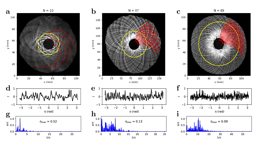
Depending on concentrations and flow rates, spatially homogeneous Brau2017 or fingered precipitation patterns Schuszter2016 ; Schuszter2016b can be obtained. In a given zone of the parameter space, the precipitate pattern features a phyllotactic–like structure (Fig. 1). To estimate the number and of right and left turning spirals in each pattern, we compute the luminosity of the pixels belonging to the circular path highlighted in yellow in Figs. 1a–c as a function of their angular position (see Figs. 1d–f). Next, we perform a Fast Fourier transform of (Figs. 1g–i), and use the position of the maximum to estimate the angular spacing between two successive spirals. The value of is then used to estimate the number of spirals as for each pattern (see top of 1a–c). We find that in those chemical precipitation phyllotactic patterns, which provides highly symmetric spatial structures. This number of spirals increases with the injection flow rate and is larger than in botanical phyllotactic patterns.
We propose that the mechanism for the formation of these spiralling precipitation patterns is due to the slaving of the precipitation process to the progression of the front which controls the local amount of solid product C Antal1999 . Identifying the equivalent of seeds in plants repulsing each other to the spatial organization of precipitate domains that segregate following an energy minimisation principle allows to understand that the solid phase appears in a phyllotactic manner when associated to the radial growth.
III Phyllotaxy in a phase separation model
Inspired by these experiments, we find that similar phyllotactic patterns can be obtained in a Cahn–Hilliard (CH) model of phase separation slaved to an front Antal1999 ; Dayeh2014 . This model is a reactive version of the classical CH equation used to describe pattern formation in spinodal decomposition Cahn1958 ; Cahn1961 , diblock copolymer segregation Tang2005 , multiphase fluid flows Cueto-Felgueroso2014 , microstructures with elastic inhomogeneities Hu2001 , or tumor growth Ebenbeck2021 , to name a few. Here, we integrate numerically the 2D reactive CH model in the sub-critical regime and in a radial geometry to model the precipitation of a species generated in the wake of an front during the radial injection of the reactant into a pool of . The dimensionless model reads (see the Supplementary Information SI section LABEL:ssec:CH_adim):
| (1a) | ||||
| (1b) | ||||
| (1c) | ||||
where is the material derivative, is the imposed volumetric flow, and is the rescaled concentration of with the diluted phase and the precipitate. The coupling between the front dynamics and precipitation is due to the source term in Eq.(1c), which takes this simple form in the limit where the reaction rate is much faster than transport (see LABEL:sec:prec_kinetic). As seen in experiments, the precipitate is assumed not to be advected once formed. The coefficients and determine the boundaries and , between the stable, metastable and unstable regions of the CH dynamics, while quantifies the boundary interaction energy between different phases and controls the typical wavelength of the phase separation pattern:
| (2) |
as predicted by linear stability analysis around a spatially homogeneous solution .
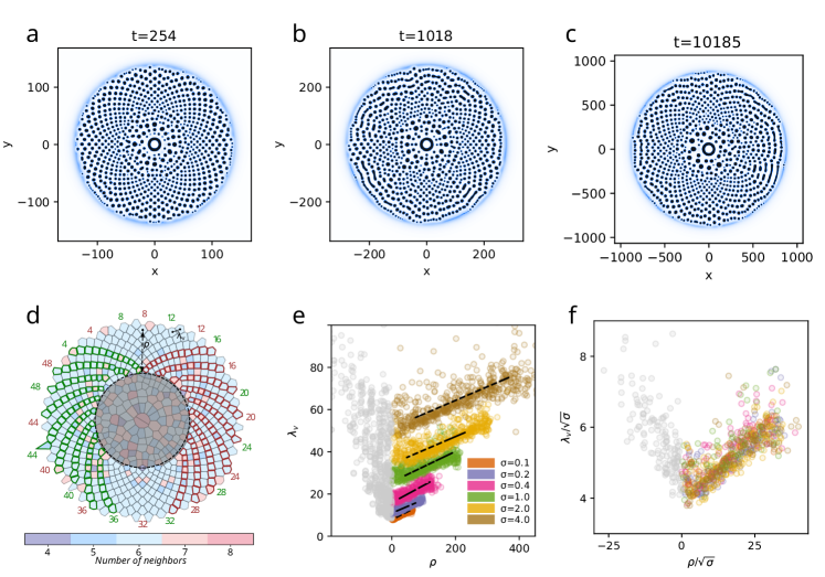
Fig. 2a–c show the numerical precipitation patterns obtained for three different values of with advective–diffusive radial transport. Strikingly, the spatial self-organization of is reminiscent of phyllotactic patterns. Increasing the value of increases the characteristic wavelength of the pattern as shown in Fig. 2e but its global shape remains self-similar, i.e. the number of parastichies remains approximately the same. Similarly to the experimental structures (Figs. 1a–c), CH patterns develop radially from the center while new spots are formed along the outer expanding circular reaction front and do not move once formed (see movie S2). The radius of the circular front position scales as (see Fig. SLABEL:sfig:CH_R_t), which is the signature of diffusive radial transport for constant volumetric flow rate advection, i.e. . This indicates that the phase transition is slaved to the radial reaction front dynamics controlled by Eqs.(1a) and (1b). Some characteristic late time coarsening is observed near the inlet region Chakrabarti1993 .
Fig. 2d shows the Voronoi diagram of the pattern displayed in Fig. 2a. Outside the coarsening region, the spots are mainly arranged on an hexagonal lattice as confirmed by the histograms shown in Fig. SLABEL:sfig:CHneig. This result shows that the selection of a certain spiralling mode responds to a spot packing optimisation criterion scenario Douady1996b and, consistently, the number of left and right turning spirals is the same (see Fig. 2d), i.e. the observed patterns have no chirality.
In the general picture proposed by Golé et al. Gole2016 , the number of spirals is controlled by the dimensionless number , being the perimeter of the front where new spots appear and the distance between two spots on the front. Here, spots appear on peripheral circles, thus while where is twice the apothem of a hexagon of area and is the area of the Voronoi cells (Fig. 2d). The histogram of Fig.SLABEL:sfig:CH_scalea shows the distribution of for four different values of . In Fig. SLABEL:sfig:CH_scaleb, we observe that, if rescaled by , all histograms collapse on each other, which indicates that scales like the theoretical value (Eq.2). In Fig. 2(e), the value of is given for each Voronoi cell as a function of the radial distance , being the radius of the coarsening region. For , decreases with the radial position and is broadly distributed, which is a signature of the coarsening dynamics of earlier generated spots. Conversely, for , increases linearly with and is less broadly distributed. This shows that , the typical distance between new spots, scales linearly with the radius . Hence, is actually a constant , which explains why the number of parastichies does not change during the growth of the pattern.
Eventually, Fig. 2f shows the data of Fig. 2e rescaled by . The collapse of all curves is consistent with the results of Fig. SLABEL:sfig:CH_scaleb, i.e. what matters is only the order number of the rings of new appearing spots and the number of spots per ring. To confirm this scenario, Fig.SLABEL:sfig:CH_R_vs_na plots the front radius at different times as a function of the number of enclosed spots for different values of . If is rescaled by (Fig. SLABEL:sfig:CH_R_vs_nb), all data collapse on the same curve which means that, if time is measured in terms of the number of spots and space by unit of the instability wavelength , all the patterns are equivalent (see discussion in LABEL:ssec:ssimilar_scaling). Note that, despite this general self-similarity, both highly ordered spiralling patterns (as the one shown in Fig. 2a) and less ordered arrangements (like the one shown Fig. 2b and Fig. 2c) can be observed. This behavior is analysed in detail in the Methods and in figures SLABEL:sfig:CH_T_conv, SLABEL:sfig:CH_noise and SLABEL:sfig:CH_S_conv.
Finally, we observe that the product distribution in reactive fronts is controlled by the initial value of , and the imposed values of and at the inlet, which in our case also dictates the morphology of the expressed pattern via the source term in eq. 1c. In particular, the observation of spots instead of stripes Thiele2019 , requires the phase field to be close to the limit of linearly unstable region, i.e. . The observation of phyllotactic patterns thus requires a fine tuning of the interplay between the reaction–diffusion–advection front and the CH spatial symmetry breaking instability.
IV Reaction–diffusion Turing patterns
Phyllotactic pattern can also be obtained in another class of spatial symmetry breaking instability: Turing patterns. To show this, we consider the irreversible Brusselator model, , , , , where are the initial reactants and are the autocatalytic and the inhibitor intermediate species with diffusivities and , respectively Prigogine1968 . In extended systems with spatially homogeneous and constant reactant concentrations and (pool chemical approximation Nicolis1977 ), the coupling of the Brusselator kinetics to diffusion can produce spatial stationary Turing structures, characterized by an intrinsic wavenumber:
| (3) |
when , where . The morphology of the stationary Turing structures depends on the value of the control parameter , with hexagonally-distributed spots being the first symmetry to appear subcritically followed by supercritical stripes Dewel1995 ; DeWit1999 .
Here, we consider a heterogeneous distribution of the reactants and resulting from a radial diffusion or diffusion–advection transport of A from a circular inlet of radius , where and , into a two-dimensional sea where the reactants concentration is initially and . Neglecting the chemical consumption of A and B, the set of dimensionless equations describing such oscillator fronts reads Nicolis1977 ; Budroni2016 ; Budroni2017 :
| (4a) | ||||
| (4b) | ||||
| (4c) | ||||
| (4d) | ||||
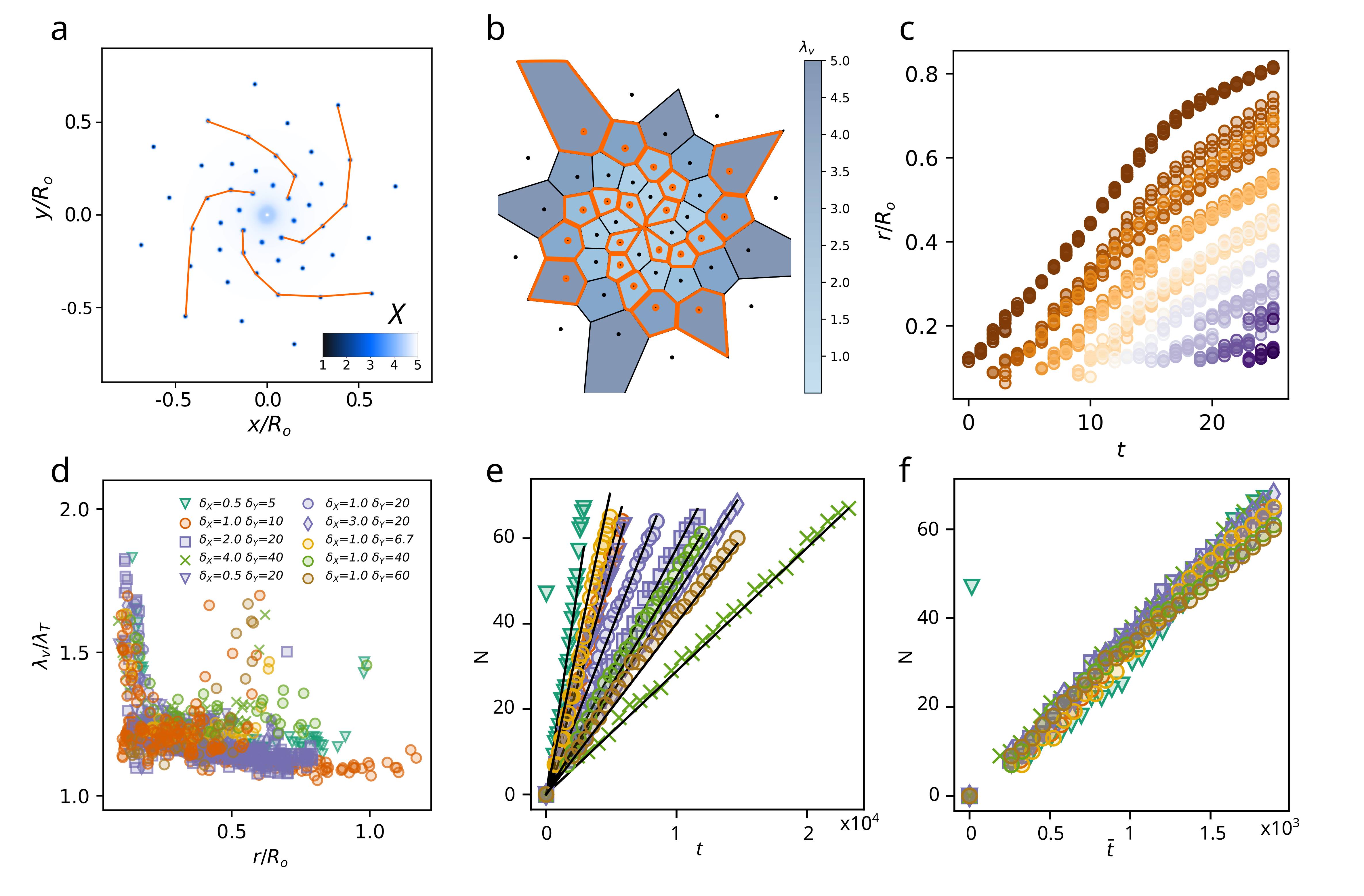
where are the dimensionless diffusion coefficients (see also Methods section). Fig.3a shows a typical Turing pattern obtained by solving numerically Eqs.(4a–4d) with . Spots of high concentration of the reaction intermediate arrange themselves along eight distinct spirals as shown in the Voronoi diagram of Fig 3b, which reminds of phyllotactic patterns. Contrarily to experimental precipitations and numerical CH patterns described above, new spots appear here close to the central injection, and successively drift away in the radial direction as shown in Fig. SLABEL:sfig:BR_traj (SI) and movie S3, even in the absence of advection (i.e. ). The distance between spots increases with the distance from the center as seen on Fig. 3b. New spots appear at a constant rate (Fig. 3e) and their drifting velocity is approximately constant as long as the spots are far from the edge of the simulation domain (Fig. 3c). The spot dynamics is therefore directly comparable to the phyllotactic movement of the magnetic droplets in Douady and Couder experiments Douady1992 even though, in the Turing patterns, the release rate of the new spots and their drift velocity cannot be directly imposed. Instead, their dynamics is here a spontaneous consequence of how spots self-organise in space with an intrinsic local wavenumber dependent on the profile as in eq. 3.
Phyllotactic Turing patterns were also observed for other sets of parameters as summarised in Table SLABEL:stab:Bru_simulations and Fig. SLABEL:sfig:BR_diapo and Fig. SLABEL:sfig:BR_Q_var (SI). By varying the values of and , we found that the spot dynamics is entirely controlled by the transport of reactant via the local value of the Turing wavelength , also in the presence of advection (i.e. ).
To prove it, we show in Fig 3d the ratio between the local distance between spots (computed as in the previous section) as a function of the radial position and and observe that all points of each simulation collapse on the same horizontal line at . Finally, to prove that the appearance rate of new spots is controlled by the value of and , we plot in Fig. 3f the number of spots as a function of a rescaled time . For all simulations performed (see Table SLABEL:stab:Bru_simulations), the data collapse on the same straight line.
Note that, as for the CH simulations, the dimensionless number remains constant for the Brusselator patterns, coherently with a number of spirals remaining also constant. However, differently from CH simulations, here stays constant because new spots appear in the center, on a circle of approximately constant radius as shown in Fig. SLABEL:sfig:BR_trajb, jointly to the negligible variation of as shown in Fig. SLABEL:sfig:1point_lambda.
V Phyllotactic spatial symmetry-breaking patterns
Despite the differences in their dynamics and in the nature of the spatial symmetry-breaking instability producing the pattern, phyllotactic structures observed in the phase separation CH model and in the reaction–diffusion Brusselator model show important similarities. First, in both cases, the pattern selection is tightly controlled by the instability wavelength , through the dimensionless number . In particular, we find that is always a function of , i.e. . In all scenarios explored here, turns actually to be a constant but we expect that other scenarios may exist where is not constant.
Another strong similarity is that, in both models and in the precipitation experiments as well, the observed patterns belong to the family of the ”whorled modes”, i.e. phyllotactic structures where the number of left and right turning spirals is the same. Interestingly, while much less abundant in extant plants as compared to Fibonacci spiral modes, whorled modes may have not been the exception in ancestral plants Turner2023 and are observed next to spiral modes Schoute1922 ; Douady1996b . Moreover, accordingly to Douady1996b : 1) whorled modes always develop by the appearance of multiple new primordia at once and 2) the selection of whorled or spiral modes is driven by a criterion of packing optimisation. In the present work, we confirm that both 1) and 2) are retrieved. Indeed, groups of new spots appear simultaneously on circular fronts in all our experiments and simulations. Also we showed, by using Voronoi diagrams, that phyllotactic patterns observed in CH and Brusselator models arrange themselves on a hexagonal lattice, which corresponds to the most efficient packing solution in 2D.
If our results appear consistent with previous explorations, one question remains, which is: can one observe spiral modes and Fibonacci transitions in phyllotactic patterns driven by a symmetry-breaking instability in radial geometries, such as those presented here? According to the general approach proposed by Golé et al. Gole2016 , the selection between whorled (or quasi-symmetric) and spiral modes is controlled by the initial noise and the rate of change of . Unfortunately, this hypothesis could not be tested in the minimal model systems presented here because was always constant, which means that whorled modes are attractors Gole2016 .
More generally, we remark that the development of a spatial symmetry-breaking instability is inevitably frustrated in a spatial domain whose typical length is smaller than the instability’s intrinsic wavelength. As a consequence, the corresponding pattern cannot appear but across a region that spans at least some wavelengths. Thus, the simultaneous appearance of new primordia may be intrinsic to phyllotactic patterns driven by symmetry-breaking instabilities and restrict the access to modes other than whorled modes, which is coherent with previous literature (Douady1996b, , and citations therein).
To conclude, we have shown that phyllotactic patterns can appear when a spatial symmetry-breaking instability is coupled to the dynamics of a radially growing reaction front. Specifically, spots self-organized along symmetric ontogenic spirals have been obtained experimentally in the wake of a chemical precipitation front and in models of both phase transition and Turing self-organisation when one reactant controlling the dynamics of the reaction front is radially transported into the other one. The genericity of the systems analysed, suggests that the observed spiraled patterns belong to a new class of phyllotactic growth structures, that we encourage to explore in the vast class of spatial symmetry-breaking instabilities as observed in a wide range of fields from chemistry Castets1990 to optics Haudin2014 and biology Nakamasu2009 ; Budrene1995 .
VI Methods
Analysis of experimental patterns Experimental patterns were analysed using the Python library SciPy. For each experimental image, we manually identify a circular path, centered in the inlet, where the luminosity signal shows a good contrast. Next, we select all the pixels (highlighted in yellow in Figs. 1a–c) which belong to an annular region which is 4 pixels thick and is centered on the circular path. We then report the luminosity of each pixel as a function of their azimuthal position and perform a moving average of . Next, we perform a linear 1D interpolation of in order to have a regularly sampled signal (see Figs. 1d–f) and perform a Fast Fourier transform (Figs. 1g–i). Finally, we manually identify the maximum of the FFT signal and use the maximum position to estimate the angular distance between two successive spirals.
Cahn-Hilliard model. Equations (1a-1c) were solved in two steps. First, we solve the reaction–diffusion–advection equation (1a-1b) in a 1D axisymmetric high resolution domain [,] using the finite elements solver COMSOL Multiphysics and store the value of the source term as a function of and . For the reactant concentrations and , boundary conditions were no-flux at the outer boundary and Dirichlet at the inner boundary where we fix and . The velocity field was considered as stationary and axisymmetric, i.e. , where is simply because the flow is supposed laminar and incompressible.
Next, we solve the CH equation (1c) using a homemade finite differences code written in Python in a 2D square grid domain of side . The value of was computed for each grid point and time step by using the linear interpolation function provided by the Python library SciPy and no-flux boundary conditions were imposed at the outer boundaries. Our investigations showed that the observed pattern is extremely sensitive to the initial conditions which can strongly affect the degree of ”ordering” of the final spiralling patterns as mentioned in the results section. This feature emerged when conducting convergence tests on our simulations. In particular, while time convergence is well verified (see Fig. SLABEL:sfig:CH_T_conv), i.e. identical patterns are obtained by taking half the time-step, we face a more complex scenario for spatial convergence. Indeed, in certain runs it is sufficient to change the gridstep to observe a significant rearrangement of spirals and even the disruption of part of them, which corresponds to patterns similar to those presented in Figs. 2b and 2c, while the overall scaling of the pattern is always preserved (Figs. 2e and 2f).
Convergence study In order to investigate this behaviour and rule out the possibility that our simulations were not well resolved, we proceeded in the following way (see SI section LABEL:ssec:numerical_convergence for more details). First, we add some random noise to the source term and repeat the same simulation as in Figs. 2a-b by only changing the noise seed as shown in Fig. SLABEL:sfig:CH_noise. Second, we initialize some simulations with the pattern taken at short time from different simulations with the same parameters (including noise) but at different spatial resolution as shown in Fig. SLABEL:sfig:CH_S_conv. We observed that:
-
•
low amplitude noise, i.e. times smaller than the source amplitude, is sufficient to modify the final spiralling pattern.
-
•
When initiating simulations using the pattern obtained from other simulations at early but sufficiently large time, i.e. 1/10 of the total simulation time, spatial convergence is recovered.
These two results indicate that, for a given set of parameters, multiple (genuine) solutions are possible and that their selection, as well as the degree of spirals ordering, is extremely sensitive to multiple factor including initial noise, spatial resolution and source amplitude.
Brusselator model. The set of dimensionless equations (4a-4d) is obtained using the reaction constants as defined in the system of equations LABEL:seq:brusselator_reactions. The time scale was defined as , space scale is , are the dimensionless diffusion coefficient and concentrations were rescaled as it follows: ; ; ; ; where are the dimensional concentrations. Finally, we neglected the reactive consumption of A and B, supposing that their depletion occurs on a much slower time scale as compared to that characterizing the dynamics of the chemical intermediates, as it happens, for instance, in the well-known Belousov–Zhabotinsky reaction.
Equations (4a-4d) were solved using the finite elements solver COMSOL Multiphysics. The simulation domain has the same circular shape as in CH simulations except in one simulation in a linear geometry. Space was discretized using a triangular mesh of variable size, and the maximum length of a grid element was set to 1/20 of the minimum wavelength observed in the pattern. For species A and B, boundary conditions were no-flux at the outer boundary and Dirichlet at the inner boundary where and . When the injection flow rate is non zero, the velocity field is solved in the same way as in CH simulations.
References
- (1) Jean, R. V. Phyllotaxis: A Systemic Study in Plant Morphogenesis (Cambridge University Press, Cambridge, 1994).
- (2) Adler, I. A History of the Study of Phyllotaxis. Ann. Bot. 80, 231–244 (1997).
- (3) Douady, S. & Couder, Y. Phyllotaxis as a physical self-organized growth process. Phys. Rev. Lett. 68, 2098–2101 (1992).
- (4) Hofmeister, W. Allgemeine Morphologie der Gewächse. In Handbuch der Physiologischen Botanik, vol. 1, 405–664 (Wilhelm Engelmann, Leipzig, 1868).
- (5) Richards, F. J. Phyllotaxis: Its quantitative expression and relation to growth in the apex. Phil. Trans. R. Soc. Lond. B 235, 509–564 (1951).
- (6) Douady, S. & Couder, Y. Phyllotaxis as a Dynamical Self Organizing Process Part II: The Spontaneous Formation of a Periodicity and the Coexistence of Spiral and Whorled Patterns. Journal of Theoretical Biology 178, 275–294 (1996).
- (7) Snow, M. & Snow, G. R. S. Minimum areas and leaf determination. Proc. R. Soc. B 139, 545–566 (1952).
- (8) Iterson, G. v. G. Mathematische und mikroskopisch-anatomische Studien über Blattstellungen nebst Betrachtungen über den Schalenbau der Miliolinen (Jena, Fischer, 1907).
- (9) Golé, C., Dumais, J. & Douady, S. Fibonacci or quasi-symmetric phyllotaxis. Part I: Why? Acta Soc. Bot. Pol. 85 (2016).
- (10) Cross, M. C. & Hohenberg, P. C. Pattern formation outside of equilibrium. Rev. Mod. Phys. 65, 851–1112 (1993).
- (11) Brau, F., Schuszter, G. & De Wit, A. Flow control of fronts by radial injection. Phys. Rev. Lett. 118, 134101 (2017).
- (12) Schuszter, G., Brau, F. & De Wit, A. Flow-driven control of calcium carbonate precipitation patterns in a confined geometry. Phys. Chem. Chem. Phys. 18, 25592–25600 (2016).
- (13) Schuszter, G., Brau, F. & De Wit, A. Calcium Carbonate Mineralization in a Confined Geometry. Environ. Sci. Technol. Lett. 3, 156–159 (2016).
- (14) Haudin, F., Cartwright, J. H. E., Brau, F. & De Wit, A. Spiral precipitation patterns in confined chemical gardens. Proc. Natl. Acad. Sci. 111, 17363–17367 (2014).
- (15) Bohner, B., Schuszter, G., Berkesi, O., Horváth, D. & Tóth, Á. Self-organization of calcium oxalate by flow-driven precipitation. Chem. Commun. 50, 4289–4291 (2014).
- (16) Ziemecka, I. et al. Polymorph Selection of ROY by Flow-Driven Crystallization. Crystals 9, 351 (2019).
- (17) Grzybowski, B. A. Chemistry in Motion: Reaction-Diffusion Systems for Micro- and Nanotechnology (Wiley, Chichester, U.K, 2009).
- (18) Knoll, P., Nakouzi, E. & Steinbock, O. Mesoscopic Reaction–Diffusion Fronts Control Biomorph Growth. J. Phys. Chem. C 121, 26133–26138 (2017).
- (19) Schuszter, G. & De Wit, A. Comparison of flow-controlled calcium and barium carbonate precipitation patterns. The Journal of Chemical Physics 145, 224201 (2016).
- (20) Antal, T., Droz, M., Magnin, J. & Rácz, Z. Formation of Liesegang Patterns: A Spinodal Decomposition Scenario. Phys. Rev. Lett. 83, 2880–2883 (1999).
- (21) Dayeh, M., Ammar, M. & Al-Ghoul, M. Transition from rings to spots in a precipitation reaction–diffusion system. RSC Adv. 4, 60034–60038 (2014).
- (22) Cahn, J. W. & Hilliard, J. E. Free Energy of a Nonuniform System. I. Interfacial Free Energy. The Journal of Chemical Physics 28, 258–267 (1958).
- (23) Cahn, J. W. On spinodal decomposition. Acta Metallurgica 9, 795–801 (1961).
- (24) Tang, P., Qiu, F., Zhang, H. & Yang, Y. Phase separation patterns for diblock copolymers on spherical surfaces: A finite volume method. Phys. Rev. E 72, 016710 (2005).
- (25) Cueto-Felgueroso, L. & Juanes, R. A phase-field model of two-phase Hele-Shaw flow. J. Fluid Mech. 758, 522–552 (2014).
- (26) Hu, S. Y. & Chen, L. Q. A phase-field model for evolving microstructures with strong elastic inhomogeneity. Acta Materialia 49, 1879–1890 (2001).
- (27) Ebenbeck, M., Garcke, H. & Nürnberg, R. Cahn–Hilliard–Brinkman systems for tumour growth. DCDS-S 14, 3989–4033 (2021).
- (28) Chakrabarti, A., Toral, R. & Gunton, J. D. Late-stage coarsening for off-critical quenches: Scaling functions and the growth law. Phys Rev E 47, 3025–3038 (1993).
- (29) Thiele, U., Frohoff-Hülsmann, T., Engelnkemper, S., Knobloch, E. & Archer, A. J. First order phase transitions and the thermodynamic limit. New J. Phys. 21, 123021 (2019).
- (30) Prigogine, I. & Lefever, R. Symmetry Breaking Instabilities in Dissipative Systems. II. The Journal of Chemical Physics 48, 1695–1700 (1968).
- (31) Nicolis, G. & Prigogine, I. Self-organization in non equilibrium systems : From dissipative structures to order through fluctuations (Wiley, New York NY, 1977).
- (32) Dewel, G. et al. Pattern selection and localized structures in reaction-diffusion systems. Physica A: Statistical Mechanics and its Applications 213, 181–198 (1995).
- (33) De Wit, A. Spatial Patterns and Spatiotemporal Dynamics in Chemical Systems. In Advances in Chemical Physics, 435–513 (John Wiley & Sons, Ltd, 1999).
- (34) Budroni, M. A. & De Wit, A. Localized stationary and traveling reaction-diffusion patterns in a two-layer A + B oscillator system. Phys. Rev. E 93, 062207 (2016).
- (35) Budroni, M. A. & De Wit, A. Dissipative structures: From reaction-diffusion to chemo-hydrodynamic patterns. Chaos 27, 104617 (2017).
- (36) Turner, H.-A., Humpage, M., Kerp, H. & Hetherington, A. J. Leaves and sporangia developed in rare non-Fibonacci spirals in early leafy plants. Science 380, 1188–1192 (2023).
- (37) Schoute, J. C. On Whorled Phyllotaxis. I Growth Whorls. Recl. Trav. Bot. Néerl. 19, 184–206 (1922).
- (38) Castets, V., Dulos, E., Boissonade, J. & De Kepper, P. Experimental evidence of a sustained standing Turing-type nonequilibrium chemical pattern. Phys. Rev. Lett. 64, 2953–2956 (1990).
- (39) Nakamasu, A., Takahashi, G., Kanbe, A. & Kondo, S. Interactions between zebrafish pigment cells responsible for the generation of Turing patterns. Proc. Natl. Acad. Sci. U.S.A. 106, 8429–8434 (2009).
- (40) Budrene, E. O. & Berg, H. C. Dynamics of formation of symmetrical patterns by chemotactic bacteria. Nature 376, 49–53 (1995).