Learning-Augmented Robust Algorithmic Recourse

Abstract

The widespread use of machine learning models in high-stakes domains can have a major negative impact, especially on individuals who receive undesirable outcomes. Algorithmic recourse provides such individuals with suggestions of minimum-cost improvements they can make to achieve a desirable outcome in the future. However, machine learning models often get updated over time and this can cause a recourse to become invalid (i.e., not lead to the desirable outcome). The robust recourse literature aims to choose recourses that are less sensitive, even against adversarial model changes, but this comes at a higher cost. To overcome this obstacle, we initiate the study of algorithmic recourse through the learning-augmented framework and evaluate the extent to which a designer equipped with a prediction regarding future model changes can reduce the cost of recourse when the prediction is accurate (consistency) while also limiting the cost even when the prediction is inaccurate (robustness). We propose a novel algorithm for this problem, study the robustness-consistency trade-off, and analyze how prediction accuracy affects performance.

1 Introduction

Machine learning models are nowadays widely deployed even in sensitive domains such as lending or hiring. For example, financial institutions use these models to determine whether someone should receive a loan. Given the major impact that such decisions can have on people’s lives, a plethora of recent work in responsible machine learning aims to make these models fair [9, 4, 66, 26], transparent [36, 52], and explainable [51, 39, 55]. A notable line of work along this direction called algorithmic recourse [61, 58, 31], provides each individual who was given an undesirable label (e.g., one whose loan request was denied) with a minimum cost improvement suggestion to achieve the desired label.

One important weakness of much of the work on algorithmic recourse is the assumption that models are fixed and do not change [61, 58]. In practice, many models are periodically updated to reflect the changes in data distribution or the environment, which can cause the recourse to become invalid, i.e., following it may not lead to a desirable outcome [15]. To alleviate this problem, Upadhyay et al. [57] proposed a recourse framework that is robust to adversarial changes to the model parameters and provided an algorithm called ROAR to compute robust recourses. Subsequently, Nguyen et al. [44] proposed another algorithm (RBR for short) to improve ROAR’s performance for non-linear models. While both of these works computer recourses less sensitive to adversarial model changes, this comes at the price of higher cost.

To overcome this issue, we revisit the algorithmic recourse problem through the lens of the learning-augmented framework [43] which has been used in a surge of recent work to overcome the limitations of adversarial (i.e., worst-case) analysis. Specifically, rather than assuming that the designer has no information regarding how the model can change, we assume the designer can formulate predictions regarding what these changes may be. However, crucially, these predictions are unreliable and can be arbitrarily inaccurate. Using the learning-augmented approach, our goal is to optimize the validity-cost trade-off by computing recourses that perform near-optimally when the predictions are accurate (consistency) while maintaining good performance even in the worst-case, i.e., even when the predictions are arbitrarily inaccurate (robustness).

Our Results

In Section 3, we adapt the learning-augmented framework to algorithmic recourse, and our first result (Section 3.1) is a computationally efficient algorithm that computes a recourse with optimal robustness for generalized linear models. This is a non-convex problem and, to the best of our knowledge, this is the first optimal algorithm for any robust recourse problem. For non-linear models, we first approximate the model with a local linear model and then utilize our algorithm to provide recourse for the approximate model. In Section 4.1, we empirically study the combinations of robustness and consistency that are achievable across different datasets and models. These results indicate that the trade-off between robustness and consistency is domain-dependent and can vary greatly across different datasets and models. Furthermore, apart from the extreme measures of consistency and robustness, in Section 4.1, we also study how the quality of recourse solutions returned by our algorithm degrades as a function of the prediction error. Finally, in Section 4.2 we compare our recourses to those computed by ROAR and RBR, and we observe that our recourses have higher validity than these two baselines. Furthermore, for any fixed level of validity, our recourses generally have lower costs compared to ROAR and RBR.

1.1 Related Work

The emerging literature on the interpretability and explainability of machine learning systems mainly advocates for two main approaches. The first approach aims to build inherently simple or interpretable models such as decision lists [36] or generalized additive models [62, 65]. These approaches provide global explanations for the deployed models. The second approach attempts to explain the decisions of complex black-box models (such as deep neural networks) only on specific inputs [51, 39, 55, 56, 53, 1, 34, 6, 17]. These approaches provide a local explanation of the model and are sometimes referred to as post-hoc explanations.

Recourse is a post-hoc counterfactual explanation that aims to provide the lowest cost modification that changes the prediction for a given input with an undesirable prediction under the current model [61, 58, 38, 50, 54, 47]. Since its introduction, different formulations have been used to model the optimization problem in recourse (see [60] for an overview). Wachter et al. [61] and  Pawelczyk et al. [47] considered score-based classifiers and defined modifications to help instances achieve the desired scores. On the other hand, for binary classifiers, Ustun et al. [58] required the modification to result in the desired label. Roughly speaking, the first setting can be viewed as a relaxation of the second setting and we follow the second formulation in our work.

The follow-up works on the problem study several other aspects such as focusing on specific models such as linear models [58] or decision-trees [30, 10], understanding the setting and its implicit assumptions and implications [5, 59, 18, 20], attainability or actionability [29, 45, 31, 58], imperfect causal knowledge [32], fairness in terms of cost of implementation for different subgroups [22, 24, 27] and repeated dynamics [19, 8, 17]. Extending our work to account for these different aspects of recourse is left for future work.

The most closely related works are by Upadhyay et al. [57] and Nguyen et al. [44]. We compare our approach to both papers in Section 4.2. The RoCourseNet algorithm [23] also provides robust recourse though a direct comparison with this algorithm is not possible, as it is an end-to-end approach, i.e., it simultaneously optimizes for the learned model and robust recourse while the initial model is fixed in our approach, just like in [57, 44].

In addition to the closest related work mentioned in Section 1.1, Pawelczyk et al. [48] studies how model updates due to the “right to be forgotten" can affect recourse validity. Dutta et al. [16] studied the robustness in recourse for tree-based ensembles. Dominguez-Olmedo et al. [15] showed that minimum cost recourse solutions are provably not robust to adversarial perturbations in the model and then present robust recourse solutions for linear and differentiable models. Black et al. [11] observe that recourse in deep models can be invalid by small perturbations and suggest that the model’s Lipschitzness at the counterfactual point is the key to preserving validity. Very recently, Hamman et al. [25] proposed a new notion of model change which they coin “naturally-occurring" model change and provide recourse with theoretical guarantees on the validity of the recourse.

The literature on recourse is also closely related to the vast body of work on robust machine learning [41, 63, 3]. Pawelczyk et al. [46] studied the connections between various recourse formulations and their analogs in the robust machine-learning literature.

The learning-augmented framework has been applied to a wide variety of settings, aiming to provide a refined understanding of the performance guarantees that are achievable beyond the worst case. One of the main application domains is the design of algorithms (e.g., online algorithms [40, 49]), but it has also been used toward the design of data structures [35], mechanisms interacting with strategic agents [2, 64], and privacy-preserving methods for processing sensitive data [33]. This is already a vast and rapidly growing literature; see [37] for a frequently updated and organized list of related papers.

2 Preliminaries

Consider a predictive model $f_{\theta}:\mathcal{X}\to\mathcal{Y}$, parameterized by $\theta\in\Theta\subseteq\mathbb{R}^{d}$, which maps instances (e.g., loan applicants) from a feature space $\mathcal{X}\subseteq\mathbb{R}^{d}$ to an outcome space $\mathcal{Y}=\{0,1\}$. The values of 0 and 1 represent undesirable and desirable outcomes (e.g., loan denial or approval), respectively. If a model $f_{\theta_{0}}$ yields an undesirable outcome for some instance $x_{0}\in\mathcal{X}$, i.e., $f_{\theta_{0}}(x_{0})=0$, the objective in recourse is to suggest the least costly way to modify $x_{0}$ (e.g., how an applicant should strengthen their application) so that the resulting instance $x^{\prime}$ would achieve the desirable outcome under $f_{\theta_{0}}$. Given a cost function $c:\mathcal{X}\times\mathcal{X}\to\mathbb{R}_{+}$ that quantifies the cost of this transformation from $x_{0}$ to $x^{\prime}$, the recourse is defined with the following optimization problem [57]:

$$\min_{x^{\prime}\in\mathcal{X}}\ell\left(f_{\theta_{0}}(x^{\prime}),1\right)+\lambda\cdot c\left(x^{\prime},x_{0}\right),$$ (1)

where $\ell:\mathbb{R}\times\mathbb{R}\to\mathbb{R}_{+}$ is a loss function (such as binary cross entropy or squared loss) that captures the extent to which the condition $f_{\theta_{0}}(x^{\prime})=1$ is violated and $\lambda\geq 0$ is a regularizer that balances the degree of violation from the desirable outcome and the cost of modifying $x_{0}$ to $x^{\prime}$. The regularizer $\lambda$ can be decreased gradually until the desired outcome is reached. In this work, following the approach of [57, 50], we assume the cost function is the $L^{1}$ distance i.e. $c(x,x^{\prime})=\|x-x^{\prime}\|_{1}$. This implies that all the features are manipulable, they can be changed independently, and the cost of manipulating each feature is the same. We also assume the loss function $\ell$ is convex and decreasing in its first argument, which is satisfied by many commonly used loss functions such as binary-cross entropy or squared loss.

We denote the total cost of a given recourse $x^{\prime}$ for a given model $\theta$ using

$$J(x_{0},x^{\prime},\theta,\lambda)=\ell\left(f_{\theta}(x^{\prime}),1\right)+\lambda\cdot c(x^{\prime},x_{0}).$$ (2)

To further simplify notation, we ignore the dependence of $J$ on $x_{0}$ and $\lambda$ and write $J(x^{\prime},\theta)$ instead.

The objective defined in Equation (1) assumes that the parameters of the model remain the same over time, but this does not capture the fact that, in practice, predictive models may be periodically retrained and updated [57]. These updates can cause a recourse that is valid in the original model (i.e., one that would lead to the desirable outcome in that model) to become invalid in the updated model [16, 11]. It is, therefore, natural to require a recourse solution whose validity is robust to (slight) changes in the model parameters.

In line with prior work on robust recourse [57, 11], we assume that the parameters of the updated model can be any $\theta^{\prime}\in\Theta_{\alpha}$, where $\Theta_{\alpha}\subseteq\Theta$ is a “neighborhood” around the parameters, $\theta_{0}$, of the original model. Specifically, this neighborhood is defined using the $L^{\infty}$ distance and a parameter $\alpha$, so that a. Given $\theta_{0}$ and $\Theta_{\alpha}$, the robust solution would be to choose a recourse $x_{r}$ that minimizes the total cost assuming the parameters of the updated model $\theta^{\prime}\in\Theta_{\alpha}$ are chosen adversarially, i.e.,

$$x_{r}\in\arg\min_{x^{\prime}\in\mathcal{X}}\leavevmode\nobreak\ \max_{\theta^{\prime}\in\Theta_{\alpha}}J(x^{\prime},\theta^{\prime}).$$ (3)

See Section 5 for a discussion regarding alternative ways of defining model change.

3 Learning-Augmented Framework for Robust Recourse

Choosing the robust recourse $x_{r}$ according to $\eqref{eq:xr}$ optimizes the total cost against an adversarially chosen $\theta\in\Theta_{\alpha}$, but this total cost may be much higher than the optimal total cost in hindsight, i.e., if we knew the new model parameters, $\theta^{\prime}$. This is due to the overly pessimistic assumption that the designer has no information regarding what the realized $\theta^{\prime}\in\Theta_{\alpha}$ may be. Aiming to overcome similarly pessimistic results in a variety of other domains, a surge of recent work has used the learning-augmented framework [43] to provide a more refined and practical analysis. This framework assumes the designer is equipped with some unreliable (machine-learned) prediction and then seeks to achieve near-optimal performance whenever the prediction is accurate while simultaneously maintaining some robustness even if the prediction is arbitrarily inaccurate.

We adapt the learning-augmented framework to the algorithmic recourse problem and assume that the designer can generate (or is provided with) an unreliable prediction $\hat{\theta}\in\Theta_{\alpha}$ regarding the model’s parameters after the model change. For example, in the loan approval setting, a prediction can be inferred by any information regarding whether the lender would be tightening or loosening its policy over time, or even conveying more information about the changes in the form of an exact prediction for the future model. If the designer trusts the accuracy of this prediction, then an optimal solution would be to choose a recourse $x_{c}$ that is consistent with this prediction, $\hat{\theta}$, i.e.,

$$x_{c}\in\arg\min_{x^{\prime}\in\mathcal{X}}J(x^{\prime},\hat{\theta}).$$ (4)

However, since this prediction is unreliable, following it blindly could lead to very poor robustness. To evaluate the performance of a recourse $x^{\prime}$ based on the learning-augmented framework we use the robustness and consistency measures, defined below.

Definition 3.1 (Robustness).

Given a parameter $\alpha$, the robustness of a recourse $x^{\prime}\in\mathcal{X}$ is

$$R(x^{\prime},\alpha)=\max_{\theta^{\prime}\in\Theta_{\alpha}}J(x^{\prime},\theta^{\prime})-\max_{\theta^{\prime}\in\Theta_{\alpha}}J(x_{r},\theta^{\prime}),$$ (5)

where $x_{r}$ is defined in Equation (3).

The robustness measure evaluates the worst-case total cost of $x^{\prime}$ against an adversarial change of the model and then compares it to the corresponding total cost of $x_{r}$. The robustness is always at least zero (since $x_{r}$ could always be chosen as the proposed recourse $x^{\prime}$) and lower robustness values are more desirable. Note that [57] measure robustness in absolute terms, but we evaluate it relative to $x_{r}$ to enable a more direct comparison between robustness and consistency.

Definition 3.2 (Consistency).

Given a prediction $\hat{\theta}\in\Theta_{\alpha}$, the consistency of a recourse $x^{\prime}\in\mathcal{X}$ is

$$C(x^{\prime},\hat{\theta})=J(x^{\prime},\hat{\theta})-J(x_{c},\hat{\theta}),$$ (6)

where $x_{c}$ is defined in Equation (4).

The consistency is also always at least zero (zero consistency can be achieved simply by using $x^{\prime}=x_{c}$, i.e., by trusting the prediction) and lower consistency values are more desirable.

Therefore, choosing $x_{r}$ guarantees an optimal robustness of zero, but it can lead to poor consistency, and choosing $x_{c}$ guarantees an optimal consistency of zero, but it can lead to poor robustness. One of our main goals in this paper is to study the achievable trade-off between robustness and consistency, and we present our experimental evaluation of this trade-off in Section 4.1.

3.1 Computing Robust and Consistent Recourses

We next propose an algorithm to compute $x_{r}$, i.e., a robust recourse that provides an optimal solution to the optimization problem of Equation (3) when the function $f_{\theta}$ is a generalized linear model. This algorithm can also be used to compute the consistent solution $x_{c}$ of Equation (4), by setting $\alpha=0$. A model is generalized linear if $f_{\theta}$ can be written as $f_{\theta}(x):=g\circ h_{\theta}(x)$, i.e., a composition of two functions, where $h_{\theta}:\mathcal{X}\to\mathbb{R}$ is a linear function mapping inputs to scores and $g:\mathbb{R}\to[0,1]$ is a non-decreasing function mapping scores to probabilities of favorable outcome (which is the label 1 in our setting). For example, setting $g$ to be the sigmoid function will recover the logistic regression.

Note that even for generalized linear functions, the objective function in (4) is non-convex (see Appendix A). Hence, gradient-based approaches such as RObust Algorithmic Recourse (ROAR) [57] or Robust Bayesian Recourse (RBR) [44] can only converge to a locally optimal recourse, as opposed to our algorithm which guarantees globally optimal recourse. We empirically compare the performance of our algorithm to these algorithms in Section 4.2.

We introduce a few additional notations. We use $\operatorname{sgn}$ to denote the function $\operatorname{sgn}(s)=\mathbbm{1}[s\geq 0]$ where $\mathbbm{1}$ is the indicator function. When applied to a vector, the $\operatorname{sgn}$ is applied element-wise to each dimension of the vector. For an integer $n\in\mathbb{N}$, $[n]:=\{1,\ldots,n\}$. We also use $e_{i}$ to denote a $d$-dimensional unit vector with all zeros except for $i$-th coordinate which has a value of one.

Input : $x_{0}$, $\theta_{0}$, $\ell$, $c$, $\alpha$

Output: $x^{\prime}$

1:  Initialize $x^{\prime}\leftarrow x_{0}$

2:  Initialize Active=$[d]$ $\triangleright$ Set of coordinates to update

3:  for  $i\in[d]$  do

4:     if $x_{0}[i]\neq 0$ then

5:        Initialize $\theta^{\prime}[i]\leftarrow\theta_{0}[i]-\alpha\cdot\operatorname{sgn}(x_{0}[i])$ $\triangleright$ Initialization for $\theta^{\prime}$ (the worst-case model)

6:     else

7:        if $|\theta_{0}[i]|>\alpha$ then

8:           Initialize $\theta^{\prime}[i]\leftarrow\theta_{0}[i]-\alpha\cdot\operatorname{sgn}(\theta_{0}[i])$

9:        else

10:           Active $\leftarrow$ Active $\setminus\{i\}$ $\triangleright$ Remove the coordinate that cannot improve $J$

11:  while $\textsc{Active}\neq\emptyset$ do

12:     $i\leftarrow\operatorname*{arg\,max}_{j\in\textsc{Active}}|\theta^{\prime}[j]|$$\triangleright$ Next coordinate to update

13:     $\Delta\leftarrow\operatorname*{arg\,min}_{\Delta}J(x^{\prime}+\Delta e_{i},\theta^{\prime})-J(x^{\prime},\theta^{\prime})$ $\triangleright$ Compute the best update for the selected coordinate

14:     if $\operatorname{sgn}(x^{\prime}[i]+\Delta)=\operatorname{sgn}(x^{\prime}[i])$ then

15:        $x^{\prime}[i]\leftarrow x^{\prime}[i]+\Delta$ $\triangleright$ Apply the update and terminate

16:        break

17:     else

18:        $x^{\prime}[i]\leftarrow 0$ $\triangleright$ Update the coordinate but only until it reaches 0

19:        if $\operatorname{sgn}(\theta_{0}[i])=\operatorname{sgn}(\theta_{0}[i]+\alpha\cdot\operatorname{sgn}(x_{0}[i]))$ then

20:           $\theta^{\prime}[i]\leftarrow\theta_{0}[i]+\alpha\cdot\operatorname{sgn}(x_{0}[i])$ $\triangleright$ Modify $\theta^{\prime}$ accordingly

21:        else

22:           Active $\leftarrow$ Active $\setminus\{i\}$

23:  return  $x^{\prime}$

ALGORITHM 1 Optimal Robust Recourse

Algorithm 1 starts by computing the worst-case model $\theta^{\prime}$ for the “default” recourse of $x_{0}$; see Lemma A.2 for why the for-loop of Algorithm 1 (lines 3-10) achieves that. Then, facing $\theta^{\prime}$, the algorithm greedily modifies $x_{0}$ into $x_{r}$ while simultaneously updating $\theta^{\prime}$ to ensure that it remains the worst-case model for the current recourse $x^{\prime}$. In each iteration of the while loop, the algorithm identifies the dimension $i$ of $\theta^{\prime}$ that has the largest absolute value (line 12) and then computes the optimal change of $x^{\prime}[i]$ if we were to keep $\theta^{\prime}$ fixed (line 13). If this change does not cause $x^{\prime}[i]$ to flip its sign, the adversary does indeed remain fixed, so $x^{\prime}$ is the optimal recourse and the algorithm terminates. On the other hand, if the recommended change would flip the sign of $x^{\prime}[i]$, this would cause the adversarial response to change as well (see Lemma A.2). The algorithm instead applies this change all the way up to $x^{\prime}[i]=0$, it updates $\theta^{\prime}$ accordingly, and repeats. If, during this process, for some dimension $i$ we have $x^{\prime}[i]=0$ and an update of the adversarial model $\theta^{\prime}[i]$ could cause its sign to flip, then no further change in this dimension is allowed ($i$ is removed from the Active set).

We next describe the optimality guarantee of Algorithm 1. We defer the full proof to Appendix A.

Theorem 3.3.

If $f_{\theta}$ is a generalized linear model, then Algorithm 1 returns a robust recourse $x^{\prime}\in\arg\min_{x\in\mathcal{X}}\leavevmode\nobreak\ \max_{\theta^{\prime}\in\Theta_{\alpha}}J(x,\theta^{\prime})$ in polynomial time.

Proof Sketch.

We start with Observation A.1, which points out that we can assume $J(x^{\prime},\theta^{\prime})$ is a function only of the cost $\|x^{\prime}-x_{0}\|_{1}$ of $x^{\prime}$ and its inner product $x^{\prime}\cdot\theta^{\prime}$ with its worst-case (adversarial) model, $\theta^{\prime}$. Specifically, it is a linear increasing function of the former and a convex decreasing function of the latter. Using this observation, we view the problem as choosing a recourse $x^{\prime}$ and suffering a cost of $\|x^{\prime}-x_{0}\|_{1}$, aiming to maximize $x^{\prime}\cdot\theta^{\prime}$, and an adversary then chooses $\theta^{\prime}$ aiming to minimize this inner product. The actual form of $J(\cdot)$ determines the extent to which we may want to trade off the cost of recourse $x^{\prime}$ for an increase in the inner product, but the convexity with respect to the inner product suggests a decreasing marginal gain with respect to the latter.

To better understand the structure of the adversarial response, Lemma A.2 shows that for any given recourse $x$, the adversarial model $\theta^{\prime}$ is essentially equal to $\theta_{0}-\alpha\cdot\operatorname{sgn}(x)$. In other words, it shifts each coordinate $i$ by $\alpha$ (the maximum shift that it is allowed while remaining within $\Theta_{\alpha}$), and the direction is determined by whether $x[i]$ is positive or negative. As a result, we can assume that the adversarial choice of $\theta^{\prime}$ for each dimension $i$ is always either $\theta_{0}+\alpha$ or $\theta_{0}-\alpha$. This also allows us to partition $\mathcal{X}$, the space of all possible recourses, into regions that would face the same adversary. Specifically, if $x$ and $x^{\prime}$ are such that $\operatorname{sgn}(x)=\operatorname{sgn}(x^{\prime})$, then their worst-case model is the same.

Our algorithm starts from $x_{0}$ and gradually changes it until it reaches the robust recourse $x_{r}$. To determine its first step, the algorithm first computes the worst-case model $\theta^{\prime}$ for $x_{0}$ using the formula provided by Lemma A.2. If we were to assume that the adversary would remain fixed at $\theta^{\prime}$ no matter how we change the recourse, then computing the optimal recourse would be easy: we would identify the dimension $j$ for which $|\theta^{\prime}[j]|$ is maximized, and we would change only this dimension of $x_{0}$. This is optimal because changing some dimension $i$ by $\Delta$ would increase our cost by $\Delta$ and increase the inner product by $\Delta\cdot|\theta^{\prime}[i]|$ against a fixed adversary. How much we should change that dimension would then be determined by solving the optimization problem in line 13. However, if this change “flipped” the sign of $x^{\prime}[i]$, this would also change the adversary, potentially compromising the optimality of $x^{\prime}$.

Our proof shows that a globally optimal recourse can be computed by myopically optimizing $x^{\prime}$ until the adversary needs to be updated, and then repeating the same process until the marginal gain in the inner product is outweighed by the marginal increase in cost. This is partly due to the fact (shown in Lemma A.4) that the order in which this myopic approach considers the dimension of the recourse to change is optimal, exhibiting a decreasing sequence of $|\theta^{\prime}[i]|$ values.

Finally, the algorithm is efficient since the while loop can only run for $2d$ iterations and the cost of each iteration is dominated by the cost of computing $\Delta$ in line 13. This latter step can be solved efficiently [12] since $\ell$ is convex and $f_{\theta}$ is a generalized linear model. ∎

While Algorithm 1 is designed for generalized linear models, it can be extended to non-linear models by first approximating $f_{\theta}$ locally. This idea has also been used in prior work [57, 58, 50]. See Section 4 for more details. Moreover, in many settings, there are constraints on the space of feasible recourses (e.g., the recourse cannot decrease age if it is a feature), or the data contains categorical features. While Algorithm 1 cannot handle such cases, similar to prior work [57, 44, 23], the recourse of Algorithm 1 can be post-processed (e.g., by projection) to guarantee feasibility.

4 Experiments

In this section, we provide experimental results with real and synthetic datasets. We first describe the datasets and implementation details, and then present our findings in Sections 4.1 and 4.2.

Datasets

We experiment on both synthetic and real-world data. For the synthetic dataset, we follow a process similar to Upadhyay et al. [57]. We generate 1000 data points in two dimensions. For each data point, we first sample a label $y$ uniformly at random from $\mathcal{Y}=\{0,1\}$. We then sample the instance corresponding to this label from a Gaussian distribution $\mathcal{N}(\mu_{y},\Sigma_{y})$. We set $\mu_{0}=[-2,-2]$, $\mu_{1}=[+2,+2]$, and $\Sigma_{0}=\Sigma_{1}=0.5\mathbb{I}$ (see Figure 1(a) in [57]). We also use two real datasets. The first dataset is the German Credit dataset [28] which consists of 1000 data points each with 7 features containing information about a loan applicant (such as age, marital status, income, and credit duration), and binary labels good (1) or bad (0) determines the creditworthiness. The second dataset is the Small Business Administration dataset [42] which contains the small business loans approved by the State of California from 1989 to 2004. The dataset includes 1159 data points each with 28 features containing information about the business (such as business category, zip code, and number of jobs created by the business) and the binary labels indicate whether the small business has defaulted on the loan (0) or not (1). For real-world data, we normalize the features. We use the datasets to learn the initial model $\theta_{0}$. Experimental result for a larger dataset is reported in Appendix B.3.

Implementation Details

We use 5-fold cross-validation in our experiments. We use 4 folds from the data to train the initial model $\theta_{0}$ and use the remaining fold to compute the recourse. The recourse is only computed for instances that receive an undesirable label (0) under $\theta_{0}$. We report average values (over folds and test instances) in all our experiments. We used logistic regression as our linear model and trained it using Scikit-Learn. As our non-linear model, we used a 3-level neural network with 50, 100, and 200 nodes in each successive layer. The neural network uses ReLU activation functions, binary cross-entropy loss, and Adam optimizer, and is trained for 100 epochs using PyTorch. The selected architecture is identical to prior work [57]. See Appendix B.1.

To generate robust or consistent recourses for linear models we implemented Algorithm 1. We used the code from [57] and [44] for ROAR and RBR’s implementation as our baselines. Similar to [57], when the model is non-linear we first approximate it locally with LIME [51] and use the local model to generate recourse with either Algorithm 1 or ROAR, resulting in potentially different parameters $\theta_{0}$ for different instances.

We next describe our choices for parameters for Algorithm 1 and ROAR. We use binary cross-entropy as the loss function $\ell$ and $L^{1}$ distance as the cost function $c$. We use $L^{\infty}$ norm to measure the closeness in the space of model parameters. In Section 4.1, we follow a similar procedure as in [57] for selecting $\alpha$ and $\lambda$. We fix an $\alpha$ and greedily search for $\lambda$ that maximizes the recourse validity under the original model $\theta_{0}$. We study the effect of varying $\alpha$ and $\lambda$ in Section 4.2 and Appendix B.4. In each experiment, we specify how $\hat{\theta}$ is selected. See our code and Appendix B.1.

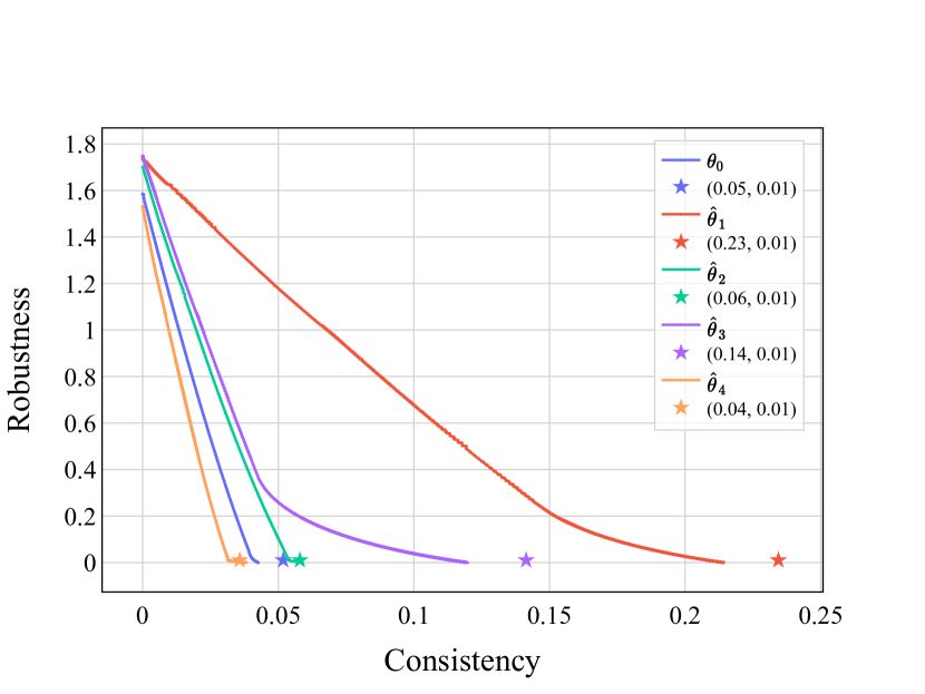
((a)) Synthetic Dataset, Logistic Regression

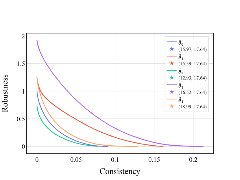
((b)) Synthetic Dataset, Neural Network

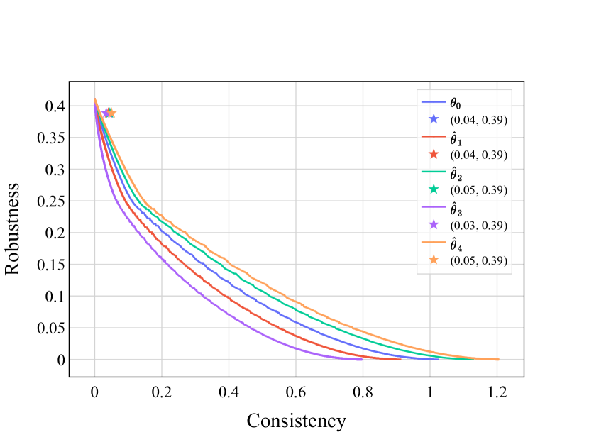
((c)) German Credit Dataset, Logistic Regression

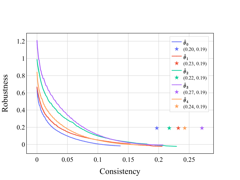
((d)) German Credit Dataset, Neural Network

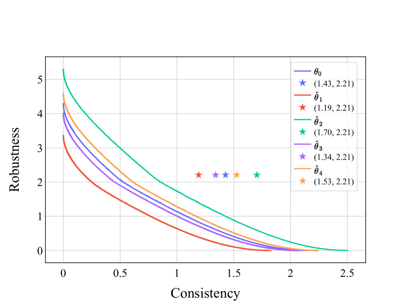
((e)) Small Business Dataset, Logistic Regression

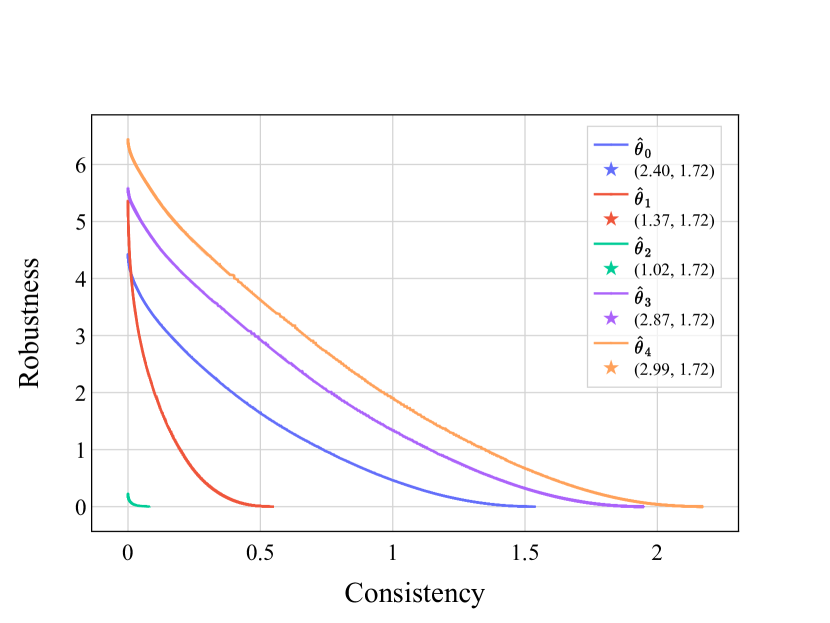
((f)) Small Business Dataset, Neural Network

Figure 1: The Pareto frontier of the trade-off between robustness and consistency for $\alpha=0.5$: logistic regression (left) and neural network (right). Rows correspond to datasets: synthetic (top), German (middle), and Small Business (bottom). In each subfigure, each curve shows the trade-off for different predictions. The robustness and consistency of ROAR solutions are mentioned in parentheses and depicted by stars. Missing stars are outside of the range of the coordinates of the figure.

4.1 Findings: Learning-Augmented Setting

Robustness-Consistency Trade-off

To study the trade-off between consistency and robustness, we generated 5 predictions. For logistic regression models, we generated 4 perturbations of the original model by adding or subtracting $\alpha$ in each dimension. For neural network models, we added the perturbation to the LIME approximation of the initial model $\theta_{0}$. Along with $\theta_{0}$, these form the 5 model parameters we used as predictions. We use $\alpha=0.5$ for the trade-off results (see Appendix B.4 for different values of $\alpha$). To compute the trade-off, for each given prediction $\hat{\theta}$, we solve for $\operatorname*{arg\,min}_{x^{\prime}}\max_{\theta^{\prime}\in\Theta_{\alpha}}\beta\cdot J(x^{\prime},\theta^{\prime})+(1-\beta)\cdot J(x^{\prime},\hat{\theta})$ for varying $\beta\in[0,1]$. To solve this optimization problem, we used a variant of Algorithm 1 (see Appendix B.2). Once, we compute the solution to this optimization problem, we can compute the robustness and consistency of the solution using Equations (5) and (6).

In Figure 1, each row corresponds to a different dataset: the synthetic dataset on the top row, the German dataset on the middle row, and the Small Business dataset on the bottom row. In the left panel, the initial model $f_{\theta_{0}}$ is a logistic regression while, in the right panel, the initial model $f_{\theta_{0}}$ is a 3-layer neural network. In each sub-figure of Figure 1, each curve shows the Pareto frontier of the trade-off between the robustness and consistency of recourses by Algorithm 1 for different predictions (indicated by different colors). The bottom right point of each curve corresponds to $\beta=1$ i.e., the optimal robust recourse $x_{r}$ which has a robustness of $0$ due to optimality of Algorithm 1 but might have different consistency depending on the prediction. Similarly, the top left point of each curve corresponds to $\beta=0$ i.e., the optimal consistent recourse with a consistency of 0. These solutions might have different robustness depending on the distance between the prediction and the worst-case model for robustness. In each subfigure, we use stars to show the robustness and consistency of the recourse provided by ROAR for each prediction. Since sometimes the stars fall outside of the coordinates of the figure we also specify the consistency and robustness of the ROAR recourse as a pair of numbers in the legend (see e.g., Figures 1(b) and 1(f)).

We observe that the sub-optimality of ROAR in terms of robustness compared to our optimal algorithm can vary greatly across different datasets and models. For example, while Figure 1(a) shows that the robustness of ROAR is only 0.01 higher than our algorithm for logistic regression models trained on the synthetic dataset, the amount of sub-optimality increases significantly to 17.64 on neural network models on the same dataset and, hence, is not displayed in Figure 1(b).

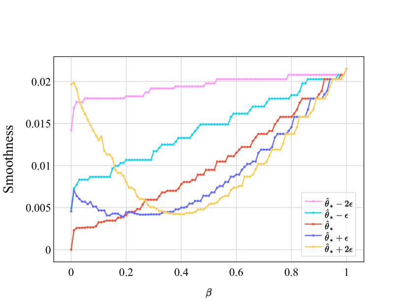
((a)) Synthetic Dataset, Logistic Regression

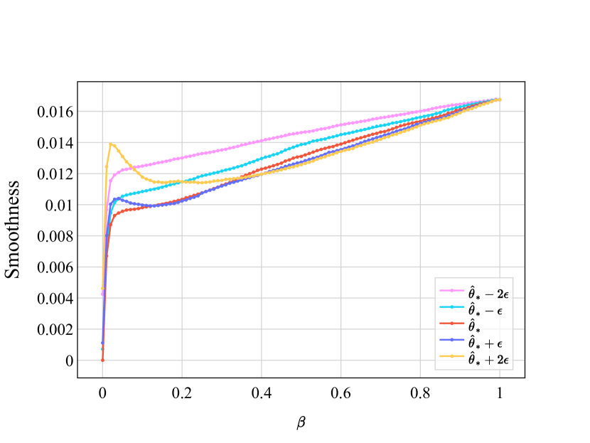
((b)) Synthetic Dataset, Neural Network

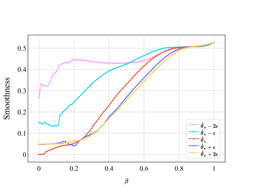
((c)) German Credit Dataset, Logistic Regression

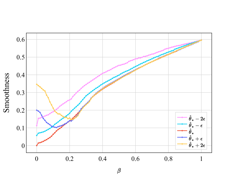
((d)) German Credit Dataset, Neural Network

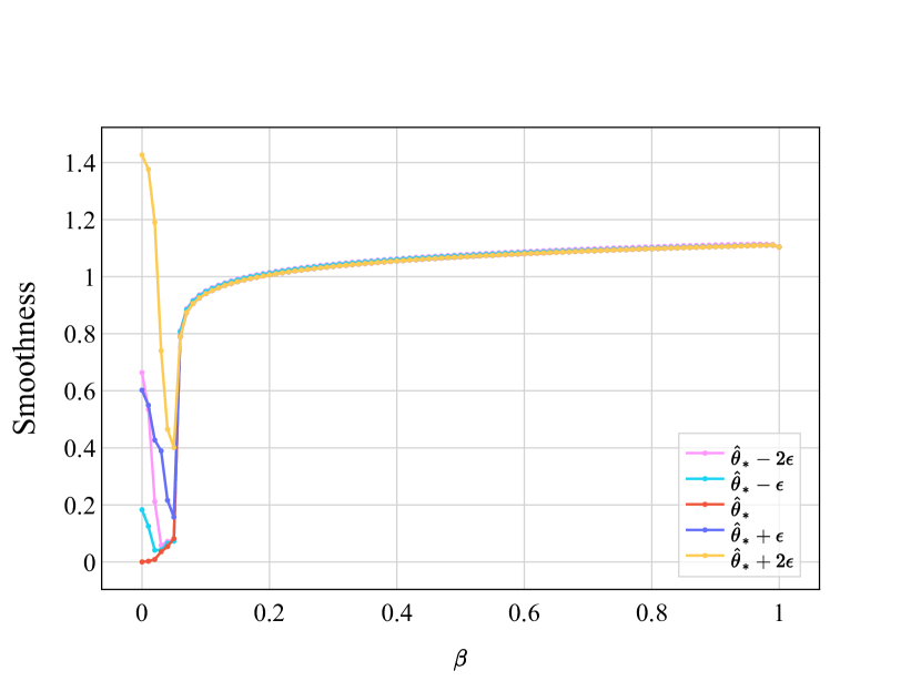
((e)) Small Business Dataset, Logistic Regression

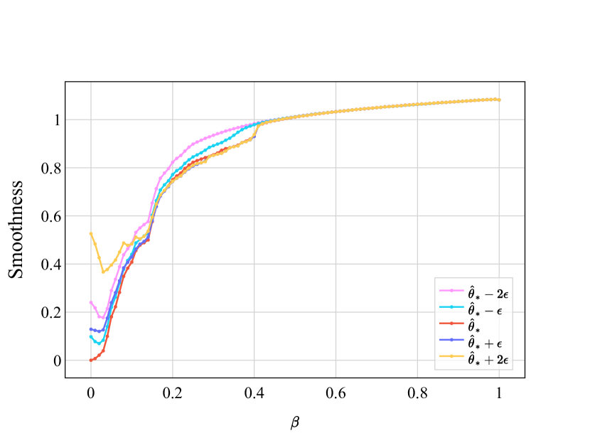
((f)) Small Business Dataset, Neural Network

Figure 2: The smoothness analysis of recourse solutions for predictions with different accuracies: logistic regression (left panel) and neural network (right panel). Rows correspond to datasets: synthetic (top), and Small Business (bottom). In each subfigure, each curve corresponds to a different prediction and tracks the total cost of the learner as a function of $\beta$ for the given prediction.

Smoothness

We also study how errors in the prediction can affect the quality of the recourse solution. In particular, for each dataset and model pair, we compute a correct prediction regarding the future model following the approach of [57]: this future model is derived by either shifting the data or as the result of temporal changes in data collection (see Appendix B.1 for more details). We then create additional, incorrect, predictions by adding perturbations to each coordinate of the correct prediction. We use four different values for the amount of added perturbations: $\{+\epsilon,-\epsilon,+2\epsilon,-2\epsilon\}$. The difference in the magnitude of perturbations allows us to generate predictions with different distances from the correct prediction: The $\epsilon$ values depend on both the dataset and the trained model and are chosen to ensure that all the predictions are within $\alpha=1$ distance of the original model. See Appendix B.1 for details.

Given a prediction $\hat{\theta}$, a learner can utilize this prediction to generate a recourse. We assume the learner solves the optimization $\operatorname*{arg\,min}_{x^{\prime}}\max_{\theta^{\prime}\in\Theta_{\alpha}}\beta\cdot J(x^{\prime},\theta^{\prime})+(1-\beta)\cdot J(x^{\prime},\hat{\theta})$ to generate a recourse. By varying $\beta$ from 0 to 1, we can simulate a diverse set of strategies for the learner: $\beta=1$ corresponds to a learner that ignores the prediction and returns the robust recourse, $\beta=0$ corresponds to a learner that fully trusts the prediction and returns the consistent solution and $\beta\in(0,1)$ simulate learners which lie in between the two extremes.

To measure the performance as a function of the prediction error, i.e., the smoothness, we use $J(x^{\prime}(\beta,\hat{\theta}),\hat{\theta}_{*})-J(x^{\prime}(\hat{\theta}_{*}),\hat{\theta}_{*})$ where $x^{\prime}(\beta,\hat{\theta})$ is the recourse returned by the learner given prediction $\hat{\theta}$ and using parameter $\beta$, $\hat{\theta}_{*}$ is the correct prediction and $x^{\prime}(\hat{\theta}_{*})$ is the consistent recourse for the correct prediction. The smoothness is non-negative and it is 0 if the learner is provided with the correct prediction ($\hat{\theta}=\hat{\theta}_{*}$) and fully trusts the prediction ($\beta=0$) to compute its recourse.

The results are summarized in Figure 2. Each row corresponds to a different dataset: synthetic (top row), German (middle row), and Small Business Administration (bottom row). The left panel shows the results for logistic regression models while the right panel corresponds to neural network models. In each sub-figure of Figure 2, each curve shows the smoothness of the learner for a given prediction as a function of $\beta$. There are 5 lines in each subfigure: one for the correct prediction (denoted as $\hat{\theta}_{*}$) and each for the four perturbations (denoted as $\hat{\theta}_{*}\pm$ the perturbation).

If we focus on $\beta=0$, we observe that the cost does, in general, increase as a function of the prediction “error” (its distance from the true model parameters: either $\hat{\theta}_{*}+2\epsilon$ or $\hat{\theta}_{*}-2\epsilon$). However, as $\beta$ increases, the total cost of recourses for different predictions converges to the same value since at $\beta=1$ the learner increasingly ignores the prediction. In some cases, this convergence occurs at smaller values of $\beta$ (e.g., Figure 2(e)) but other cases require $\beta$ to be very close to 1 (e.g., Figure 2(a)). Finally, while the total cost monotonically increases as $\beta$ increases when using the correct prediction, using incorrect predictions can result in interesting non-monotone behavior and lead to recourses that have better performance compared to using the correct prediction (e.g., Figure 2(a)).

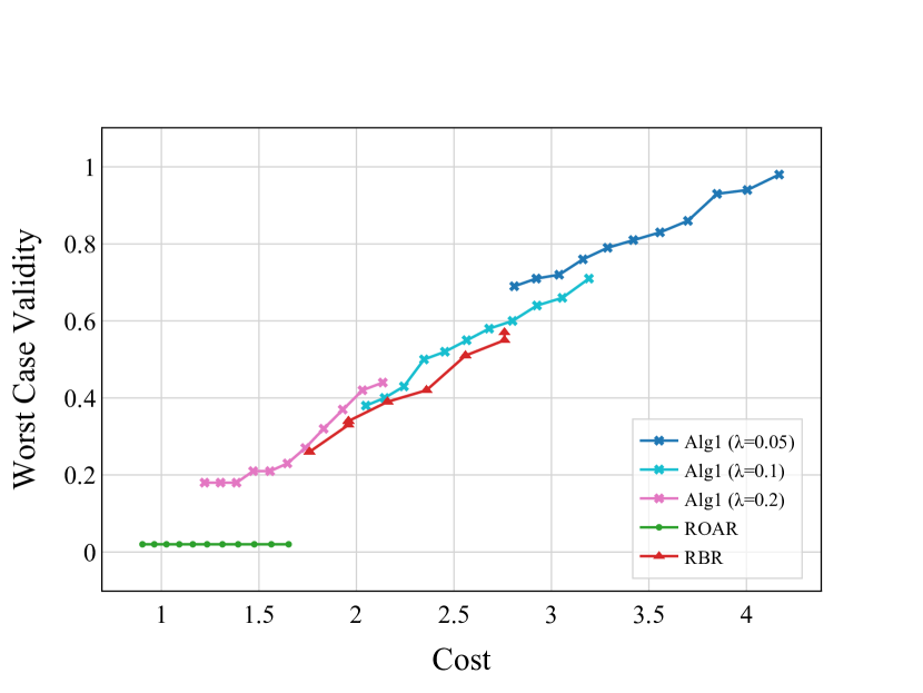
((a)) Synthetic Dataset, Logistic Regression

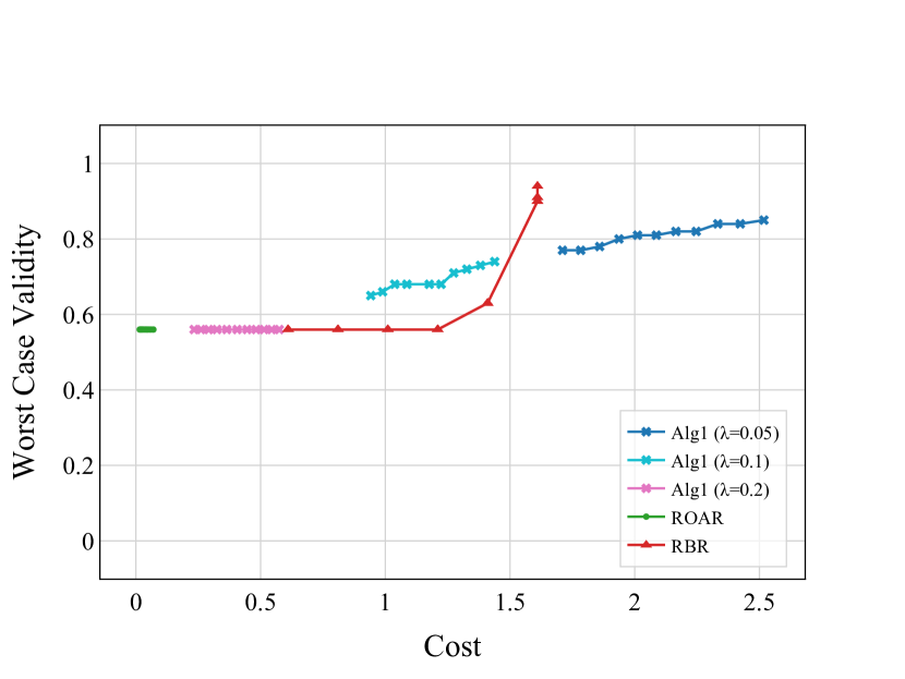
((b)) Synthetic Dataset, Neural Network

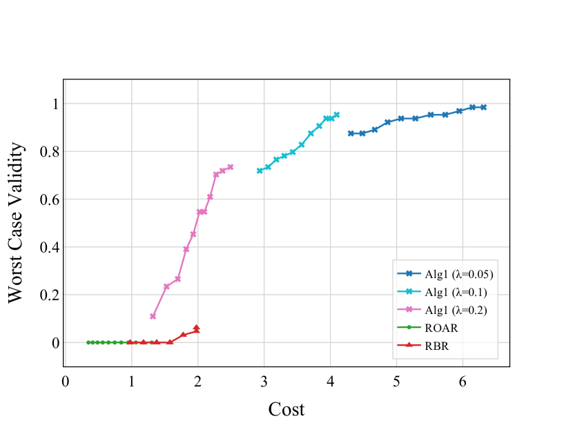
((c)) German Credit Dataset, Logistic Regression

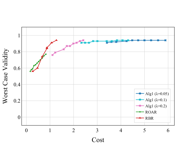
((d)) German Credit Dataset, Neural Network

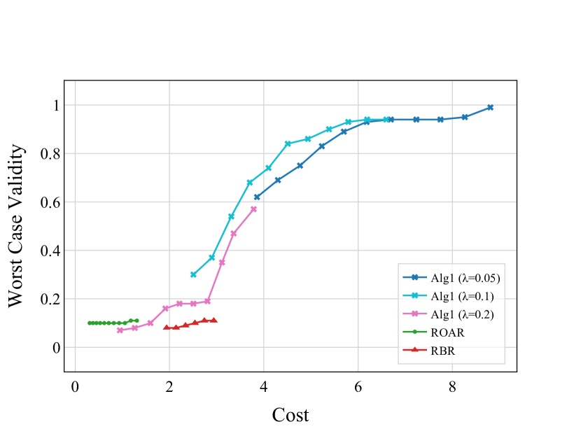
((e)) Small Business Dataset, Logistic Regression

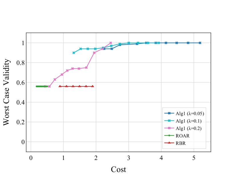
((f)) Small Business Dataset, Neural Network

Figure 3: The Pareto frontier of the trade-off between the worst-case validity and the cost of recourse solutions. The left panel is for the logistic regression while the right panel is for a 3-layer neural network. Rows correspond to datasets: synthetic (top), and Small Business (bottom). In each subfigure, each curve shows the trade-off for different methods as mentioned in the legend.

4.2 Findings: Comparison with ROAR and RBR

In Section 4.1, we showed that Algorithm 1 computes recourses with significantly smaller robustness costs compared to ROAR. In this section, we perform a more detailed comparison of our algorithm with ROAR and RBR [44] which are two main prior approaches to computing robust recourse. We first compute the robust recourse with our algorithm and these baselines. To perform a similar comparison as in prior work, we then break down the total robustness to understand the effect of each of the terms in Equation 1. The first term, $\ell\left(f_{\theta^{\prime}}(x^{\prime}),1\right)$, is a proxy for worst-case validity and the second term, $c\left(x^{\prime},x_{0}\right)$, is the cost of modifying $x_{0}$.

More formally, focusing on instances with undesirable labels under the original model $f_{\theta_{0}}$, worst-case validity is defined as the fraction of these instances labeled with the desirable label post recourse. The labels of these instances are determined using the worst-case model within $\alpha$ distance of $f_{\theta_{0}}$. This worst-case model is the one that minimizes the fraction of instances that achieve the desirable label post-recourse. We highlight that as opposed to computing a possibly different worst-case model for each instance, as is done in Sections 3 and 4.1, we compute a single worst-case model to be consistent with how validity is defined in prior work [57, 44]. We use projected gradient ascent to compute this worst-case model. See Appendix B.1.

Figure 3 depicts the Pareto frontier of the trade-off between the worst-case validity and cost of recourse for all datasets (rows) and models (columns). The Pareto frontier for RBR is obtained by varying the parameters of RBR exactly as is done in [44]. In particular, we set the ambiguity sizes $\epsilon_{1}$ and $\epsilon_{0}$ to $\epsilon_{0},\epsilon_{1}\in[0,1]$ with increments of 0.5, and the maximum recourse cost $\delta=\|x_{0}-x_{r}\|_{1}+\delta_{+}$ to $\delta_{+}\in[0,1]$ with increments of 0.2. The Pareto frontier for Algorithm 1 and ROAR is computed by varying $\alpha\in[0.02,0.2]$ in increments of 0.02. For ROAR and our algorithm, we used three different $\lambda$s: 0.05, 0.1, and 0.2, and the trade-off for each choice is plotted with a different color. To avoid overcrowding, we only included the results of $\lambda=0.05$ for ROAR. Increasing $\lambda$ to 0.1 does not change the trade-off and $\lambda=0.2$ degrades the validity even further.

For logistic regression models (left panel in Figure 3), where the optimal worst-case model can be computed efficiently, our algorithm (regardless of choice of $\lambda$) almost always dominates RBR and ROAR in terms of both cost and worst-case validity. The validity of RBR and ROAR remains low over all datasets specifically in real-world datasets. On the other hand, our algorithm displays a wide range for validity: low for $\lambda=0.2$ to almost 1 for $\lambda=0.05$. Consistent with prior work [47], the cost of the recourse increases significantly for validity values that reach 1.

For neural network models (right panel in Figure 3), gradient ascent is not guaranteed to find the optimal worst-case model. Perhaps due to this, we observe that the worst-case validity of RBR and ROAR are improved for neural network models compared to the logistic regression models. However, the validity is still generally lower compared to ours (except for Figure 3(b)). The worst-case validity of our algorithm for neural network models improves for high $\lambda$s but degrades slightly for low $\lambda$s, compared to logistic models. However, the cost of recourse is generally lower for all algorithms perhaps again due to the challenge of computing the optimal worst-case model [23].

5 Conclusion and Discussion

We initiated the study of the algorithmic recourse problem through the learning-augmented framework. One limitation of our work is the assumption that the cost of modifying features is the same for all inputs and measured using the $L^{1}$ norm. While our framework can handle customizable weights for different inputs, using any norm as the cost function implies that the features can be modified independently and does not consider the causal relationship and dependencies between different features. Some prior work on algorithmic recourse aims to understand the actionability of the recourse solution as well as considering these casual relationships [31, 29, 45]. We leave the study of these issues as future work (see Section 1.1).

Our notion of robustness and consistency measures the performance of the algorithm against the optimal robust or consistent solution in an additive manner (similar to regret in online learning [13]). This comparison can also be done multiplicatively, similar to the competitive ratio for online algorithms [43]. We leave the computation of robust and consistent recourses under a multiplicative comparison benchmark as well as the study of their trade-off as future work. Moreover, studying a weaker notions of model change such as measuring the model change by $L^{1}$ or $L^{2}$ norm [57] or studying alternative ways of formalizing model change (see e.g., [25]) is an interesting direction for future work. Finally, we assumed the prediction about the updated model is explicitly given. In practice, the feedback about the updated model might be “weaker" or even noisy [7]. Incorporating such feedback into our framework is an exciting future work direction.

Acknowledgement

We thank Kaidi Xu for insightful discussions. Vasilis Gkatzelis was partially supported by NSF CAREER award CCF-2047907 and NSF grant CCF-2210502.

Appendix A Omitted Details from Section 3.1

Non-convexity of the Optimization Problem in Equation 3 for Linear Models

We provide a concrete example that makes it easy to verify the non-convexity of the optimization problem in Equation 3 even for linear models. Consider an instance in one dimension where $x_{0}=[1,1]$ (note that the second dimension is the unchangeable intercept), $\theta_{0}=[0,0]$, $\ell$ is squared loss, $\alpha=0.5$, and $\lambda=1$. For any recourse, $x_{r}=[x,1]$ (note that the intercept cannot change), the worst-case $\theta^{\prime}$ is of the form $[0.5\text{sign}(x),-0.5]$ since $\alpha$ is 0.5 and $\theta_{0}$ is 0 in both dimensions. The cost of recourse for $x_{r}$ can be written as $1/\left(e^{0.5x\text{sign}(x)-0.5}\right)^{2}+|x-1|$. This function is not convex.

Proof of Theorem 3.3

To prove Theorem 3.3 and verify the optimality of Algorithm 1, we first make some observations and prove some useful lemmas. Without loss of generality, throughout this section we will be assuming that $\theta_{0}[i]\neq\theta_{0}[j]$ for any two dimensions $i\neq j$.

Observation A.1.

For a fixed set of parameter values, the problem of optimizing robustness in our setting can be captured as computing a recourse $x_{r}$ aiming to minimize the value of a function $J(\cdot)$ whose value depends only on the distance cost of $x^{\prime}$, i.e., $\|x^{\prime}-x_{0}\|_{1}$, and its inner product with an adversarially chosen $\theta^{\prime}\in\Theta_{\alpha}$. Formally, our goal is to compute a recourse $x_{r}$ such that:

$$x_{r}\in\arg\min_{x^{\prime}\in\mathcal{X}}\max_{\theta^{\prime}\in\Theta_{\alpha}}J(\|x^{\prime}-x_{0}\|_{1},\leavevmode\nobreak\ x^{\prime}\cdot\theta^{\prime}).$$

Also, $J(\cdot)$ is a linear increasing function of $\|x^{\prime}-x_{0}\|_{1}$ and a convex decreasing function of $x^{\prime}\cdot\theta^{\prime}$.

Observation A.1 provides an alternative interpretation of the problem: by choosing a recourse $x^{\prime}$, we suffer a cost $\|x^{\prime}-x_{0}\|_{1}$ and the adversary then chooses a $\theta^{\prime}$ aiming to minimize the value of the inner product $x^{\prime}\cdot\theta^{\prime}$. This implies that for a given $x^{\prime}$ a choice of $\theta^{\prime}$ is not optimal for the adversary unless it minimizes this inner product. Also, it implies that among all choices of $x^{\prime}$ with the same cost $\|x^{\prime}-x_{0}\|_{1}$, the optimal one has to maximize the inner product $x^{\prime}\cdot\theta^{\prime}$ with the adversarially chosen $\theta^{\prime}$. We use this fact to prove that a recourse $x^{\prime}$ is not a robust choice by providing an alternative recourse with the same cost and a greater dot product.

Our first lemma provides additional structure regarding the optimal adversarial choice in response to any given recourse $x$.

Lemma A.2.

For any recourse $x$, the adversarial response $\theta^{\prime}=\arg\max_{\theta\in\Theta_{\alpha}}J(x,\theta)$ is such that $\theta^{\prime}[i]=\theta_{0}[i]+\alpha$ for each dimension $i$ such that $x[i]<0$ and $\theta^{\prime}[i]=\theta_{0}[i]-\alpha$ for each dimension $i$ such that $x[i]>0$. For any dimension $i$ with $x[i]=0$ we can without loss of generality assume that $\theta^{\prime}[i]\in\{|\theta_{0}[i]+\alpha|,|\theta_{0}[i]-\alpha|\}$.

Proof.

For any dimension $i$ with $x[i]=0$, it is easy to verify that no matter what the value of $\theta^{\prime}[i]$ is, the contribution of $x[i]\cdot\theta^{\prime}[i]$ to the inner product $x\cdot\theta^{\prime}$ is zero, so we can indeed without loss of generality assume that $\theta^{\prime}[i]\in\{|\theta_{0}[i]+\alpha|,|\theta_{0}[i]-\alpha|\}$. Now, assume that $x[i]<0$, yet $\theta^{\prime}[i]<\theta_{0}[i]+\alpha$, and consider an alternative response $\theta^{\prime\prime}$ such that $\theta^{\prime\prime}[i]=\theta_{0}[i]+\alpha$ and $\theta^{\prime\prime}[j]=\theta^{\prime}[j]$ for all other dimensions $j\neq i$. Clearly, $\theta^{\prime\prime}\in\Theta_{\alpha}$, since $|\theta^{\prime\prime}[i]-\theta_{0}[i]|=\alpha$ and $|\theta^{\prime\prime}[j]-\theta_{0}[j]|\leq\alpha$ for all other dimensions $j\neq i$ as well, by the fact that $\theta^{\prime}\in\Theta_{\alpha}$. Therefore, it suffices to prove that $x\cdot\theta^{\prime\prime}<x\cdot\theta^{\prime}$, as this would contradict the fact that $\theta^{\prime}=\arg\max_{\theta\in\Theta_{\alpha}}J(x,\theta)$. To verify that this is indeed the case, note that

$$x\cdot\theta^{\prime}-x\cdot\theta^{\prime\prime} =x[i]\cdot\theta^{\prime}[i]-x[i]\cdot\theta^{\prime\prime}[i]$$

$$=x[i]\cdot(\theta^{\prime}[i]-\theta^{\prime\prime}[i])$$

$$>0,$$

where the first equation use the fact that $\theta^{\prime}$ and $\theta^{\prime\prime}$ are identical for all dimensions except $i$ and the inequality uses the fact that $x[i]<0$ and $\theta^{\prime}[i]<\theta^{\prime\prime}[i]$. A symmetric argument can be used to also show that $\theta^{\prime}[i]=\theta_{0}[i]-\alpha$ for each dimension $i$ such that $x[i]>0$. ∎

Lemma A.2 shows that for any recourse $x$, an adversarial response that minimizes $x\cdot\theta^{\prime}$ is $\theta^{\prime}=\theta_{0}-\alpha\cdot\operatorname{sgn}(x)$. Our next lemma shows how the adversarial response to the initial point $x_{0}$, (i.e., $\theta_{0}-\alpha\cdot\operatorname{sgn}(x_{0})$) determines the direction toward which each dimension of $x_{0}$ should be changed (if at all).

Lemma A.3.

For any optimal recourse $x_{r}\in\arg\min_{x^{\prime}\in\mathcal{X}}\leavevmode\nobreak\ \max_{\theta^{\prime}\in\Theta_{\alpha}}J(x^{\prime},\theta^{\prime})$ and every coordinate $i$, it must be that $x_{r}$ raises the value of the $i$-th dimension only if the adversary’s best response to its original value is positive, and it lowers it only if the adversary’s best response to its original value is negative. Using Lemma A.2, we can formally define this as:

$$x_{r}[i]>x_{0}[i]\leavevmode\nobreak\ \leavevmode\nobreak\ \text{ only if }\leavevmode\nobreak\ \leavevmode\nobreak\ \theta_{0}[i]-\alpha\cdot\operatorname{sgn}(x_{0}[i])>0$$

$$x_{r}[i]<x_{0}[i]\leavevmode\nobreak\ \leavevmode\nobreak\ \text{ only if }\leavevmode\nobreak\ \leavevmode\nobreak\ \theta_{0}[i]-\alpha\cdot\operatorname{sgn}(x_{0}[i])<0.$$

Proof.

Assume that for some dimension $i$ we have $x_{r}[i]>x_{0}[i]$ even though $\theta_{0}[i]-\alpha\cdot\operatorname{sgn}(x_{0}[i])<0$, and let $x^{\prime}$ be the recourse such that $x^{\prime}[i]=x_{0}[i]$ while $x^{\prime}[j]=x_{r}[j]$ for all other coordinates, $j\neq i$. If $\theta^{*}$ is the adversary’s best response to $x_{r}$ and $\theta^{\prime}$ is the adversary’s best response to $x^{\prime}$, then the difference between the inner product of $x^{\prime}\cdot\theta^{\prime}$ and $x_{r}\cdot\theta^{*}$ is:

$$x^{\prime}\cdot\theta^{\prime}-x_{r}\cdot\theta^{*} =x^{\prime}[i]\cdot\theta^{\prime}[i]-x_{r}[i]\cdot\theta^{*}[i]$$

$$=x_{0}[i]\cdot(\theta_{0}[i]-\alpha\cdot\operatorname{sgn}(x_{0}[i]))-x_{r}[i]\cdot\theta^{*}[i]$$

$$\geq x_{0}[i]\cdot(\theta_{0}[i]-\alpha\cdot\operatorname{sgn}(x_{0}[i]))-x_{r}[i]\cdot(\theta_{0}[i]-\alpha\cdot\operatorname{sgn}(x_{0}[i]))$$

$$=(x_{0}[i]-x_{r}[i])\cdot(\theta_{0}[i]-\alpha\cdot\operatorname{sgn}(x_{0}[i]))$$

$$>0,$$

where the first equation uses the fact that $x^{\prime}[j]=x_{r}[j]$ for all $j\neq i$, the second equation uses the fact that $x^{\prime}[i]=x_{0}[i]$ and the fact that the adversary’s best response to $x_{0}[i]$ is $\theta_{0}[i]-\alpha\cdot\operatorname{sgn}(x_{0}[i])$, and the subsequent inequality uses the fact that the product $x_{r}[i]\cdot\theta^{*}[i]$ is at most $x_{r}[i]\cdot(\theta_{0}[i]-\alpha\cdot\operatorname{sgn}(x_{0}[i]))$ since the adversary’s goal is to minimize this product and adversary’s best response to $x_{r}[i]$ will do at least as well as the best response to $x_{0}[i]$ (which is a feasible, even if sub-optimal, response for the adversary).

We have shown that the inner product achieved by $x^{\prime}$ would be greater than that of $x_{r}$, while the cost of $x^{\prime}$ is also strictly less than $x_{r}$, since $x^{\prime}$ keeps the $i$-th coordinate unchanged. Therefore, $\max_{\theta^{\prime}\in\Theta_{\alpha}}J(x^{\prime},\theta^{\prime})<\max_{\theta^{\prime}\in\Theta_{\alpha}}J(x_{r},\theta^{\prime})$, contradicting the assumption that $x_{r}\in\arg\min_{x^{\prime}\in\mathcal{X}}\leavevmode\nobreak\ \max_{\theta^{\prime}\in\Theta_{\alpha}}J(x^{\prime},\theta^{\prime})$. A symmetric argument leads to a contradiction if we assume that $x_{r}[i]<x_{0}[i]$ even though $\theta_{0}[i]-\alpha\cdot\operatorname{sgn}(x_{0}[i])>0$. ∎

We now prove a lemma regarding the sequence of $|\theta^{\prime}[i]|$ values of the dimensions that the while loop of Algorithms 1 changes.

Lemma A.4.

Let $j_{k}$ denote the dimension chosen in line 12 of Algorithm 1 during the $k$-th execution of its while-loop, and let $v_{k}$ denote the value of $|\theta^{\prime}[j_{k}]|$ at a point in time (note that $\theta^{\prime}$ changes over time). The sequence of $v_{k}$ values are decreasing with $k$.

Proof.

Note that in the $k$-th iteration of the while-loop, line 12 of Algorithm 1 chooses $j_{k}$ so that $j_{k}=\arg\max_{j\in\textsc{Active}}|\theta^{\prime}[j]|$, based on the values of $\theta^{\prime}$ at the beginning of that iteration. As a result, if $\theta^{\prime}$ remains the same throughout the execution of the algorithm (which would happen if $\operatorname{sgn}(x_{r})=\operatorname{sgn}(x_{0})$, i.e., if none of the recourse coordinates changes from positive to negative or vice versa), then the lemma is clearly true. On the other hand, if the recourse “flips signs” for some dimension $i$, i.e., $\operatorname{sgn}(x_{r}[i])\neq\operatorname{sgn}(x_{0}[i])$, this could lead to a change of the value of $\theta^{\prime}[i]$. Specifically, as shown in Lemma A.2 and implemented in line 20 of the algorithm, the adversary changes $\theta^{\prime}[i]$ to $\theta_{0}[i]+\alpha\cdot\operatorname{sgn}(x_{0}[i])$. If that transition causes the sign of $\theta^{\prime}[i]$ to change, then dimension $i$ becomes inactive and the algorithm will not consider it again in the future. If the sign of $\theta^{\prime}[i]$ remains the same, then we can show that its absolute value would drop after this change, so even if it is considered in the future, it would still satisfy the claim of this lemma. To verify that its absolute value drops, assume that $x_{0}[i]>0$, suggesting that the algorithm has so far lowered its value to 0, which would only happen if $\theta_{0}[i]<0$ (otherwise, this change would be decreasing the inner product). Since $x_{0}[i]>0$, the new value of $\theta^{\prime}[i]$ is equal to $\theta_{0}[i]+\alpha$, and since this remains negative, like $\theta_{0}[i]$, we conclude that its absolute value decreased. A symmetric argument can be used for the case where $x_{0}[i]<0$. ∎

We are now ready to prove our main theoretical result (the proof of Theorem 3.3), showing that Algorithm 1 always returns an optimal robust recourse.

Proof of Theorem 3.3.

To prove the optimality of the recourse $x_{r}$ returned by Algorithm 1, i.e., the fact that $x_{r}\in\arg\min_{x^{\prime}\in\mathcal{X}}\leavevmode\nobreak\ \max_{\theta^{\prime}\in\Theta_{\alpha}}J(x^{\prime},\theta^{\prime})$, we assume that this is false, i.e., that there exists some other recourse $x^{*}\in\arg\min_{x^{\prime}\in\mathcal{X}}\leavevmode\nobreak\ \max_{\theta^{\prime}\in\Theta_{\alpha}}J(x^{\prime},\theta^{\prime})$ such that $\max_{\theta^{\prime}\in\Theta_{\alpha}}J(x^{*},\theta^{\prime})<\max_{\theta^{\prime}\in\Theta_{\alpha}}J(x_{r},\theta^{\prime})$, and we prove that this leads to a contradiction.

Note that since $x^{*}\in\arg\min_{x^{\prime}\in\mathcal{X}}\leavevmode\nobreak\ \max_{\theta^{\prime}\in\Theta_{\alpha}}J(x^{\prime},\theta^{\prime})$, it must satisfy Lemma A.3. Also, note that the way that Algorithm 1 generates $x_{r}$ also satisfies the conditions of Lemma A.3 (the choice of $\Delta$ in line 13 would never lead to a recourse of higher cost without improving the inner product), so we can conclude that if $x^{*}$ and $x_{0}$ were to change the same coordinate they would both do so in the same direction, i.e.,

$$\operatorname{sgn}(x^{*}[i]-x_{0}[i])=\operatorname{sgn}(x_{r}[i]-x_{0}[i]).$$

Having established that for every coordinate $i$ the values of $x^{*}[i]$ and $x_{r}[i]$ will either both be at most $x_{0}[i]$ or both be at least $x_{0}[i]$, the rest of the proof performs a case analysis by comparing how far from $x_{0}[i]$ each one of them moves:

• Case 1: $\|x^{*}-x_{0}\|_{1}=\|x_{r}-x_{0}\|_{1}$. Since $x^{*}\neq x_{r}$, it must be that $|x^{*}[i]-x_{0}[i]|>|x_{r}[i]-x_{0}[i]|$ for some $i$ and $|x^{*}[j]-x_{0}[j]|<|x_{r}[j]-x_{0}[j]|$ for some $j$. To get a contradiction for this case as well, we will consider an alternative recourse $x^{\prime}$ that is identical to $x^{*}$ except for dimensions $i$ and $j$, each of which is moved $\delta$ closer to the values of $x_{r}[i]$ and $x_{r}[j]$, respectively, for some arbitrarily small constant $\delta>0$. Formally,

  $$x^{\prime}[i]=x^{*}[i]+\delta\cdot\operatorname{sgn}(x_{r}[i]-x^{*}[i])\leavevmode\nobreak\ \leavevmode\nobreak\ \leavevmode\nobreak\ \leavevmode\nobreak\ \leavevmode\nobreak\ \leavevmode\nobreak\ \text{and}\leavevmode\nobreak\ \leavevmode\nobreak\ \leavevmode\nobreak\ \leavevmode\nobreak\ \leavevmode\nobreak\ \leavevmode\nobreak\ x^{\prime}[j]=x^{*}[j]+\delta\cdot\operatorname{sgn}(x_{r}[j]-x^{*}[j]).$$

  Note that $x^{*}$ and $x^{\prime}$ both have the same total cost since they only differ in $i$ and $j$ and

  $$|x^{*}[i]-x_{0}[i]|+|x^{*}[j]-x_{0}[j]| =|x^{\prime}[i]-x_{0}[i]|+\delta+|x^{\prime}[j]-x_{0}[j]|-\delta$$

  $$=|x^{\prime}[i]-x_{0}[i]|+|x^{\prime}[j]-x_{0}[j]|.$$

  We let $\delta$ be small enough so that the adversary’s response to $x^{*}$ and $x^{\prime}$ is the same; for this to hold it is sufficient that a value of $x^{*}$ that is strictly positive does not become strictly negative in $x^{\prime}$, or vice versa. If we let $\theta^{\prime}$ denote this adversary, then we have

  $$x^{\prime}\cdot\theta^{\prime}-x^{*}\cdot\theta^{\prime} =\left|(x^{\prime}[j]-x^{*}[j])\cdot\theta^{\prime}[j]\right|-\left|(x^{\prime}[i]-x^{*}[i])\cdot\theta^{\prime}[i]\right|$$

  $$=\delta\cdot|\theta^{\prime}[j]|-\delta\cdot|\theta^{\prime}[i]|$$

  $$=\delta\cdot(|\theta^{\prime}[j]|-|\theta^{\prime}[i]|),$$

  where the first equality uses the fact that $x^{*}$ and $x^{\prime}$ differ only on $i$ and $j$, and the fact that if we replace recourse $x^{*}$ with $x^{\prime}$, then the change of $\delta$ on the $j$-th coordinate increases the distance from $x_{0}[j]$ and thus increases the inner product, while the change of $\delta$ on the $i$-th coordinate decreases the distance from $x_{0}[i]$ and thus decreases the inner product. The second equality uses the fact that the change on both coordinates $i$ and $j$ is equal to $\delta$.

  To conclude with a contradiction, it suffices to show that $|\theta^{\prime}[j]|>|\theta^{\prime}[i]|$, as this would imply $x^{\prime}\cdot\theta^{\prime}>x^{*}\cdot\theta^{\prime}$, contradicting the fact that $x^{*}\in\arg\min_{x^{\prime}\in\mathcal{X}}\leavevmode\nobreak\ \max_{\theta^{\prime}\in\Theta_{\alpha}}J(x^{\prime},\theta^{\prime})$, since $x^{\prime}$ would require the same cost as $x^{*}$ but it would yield a greater inner product. We consider three possible scenarios: i) If Algorithm 1 in line 12 chose to change dimension $i$ facing adversary $\theta^{\prime}[i]$ before considering dimension $j$ and adversary $\theta^{\prime}[j]$, then the fact that $|x^{*}[i]-x_{0}[i]|>|x_{r}[i]-x_{0}[i]|$ implies that the algorithm did not change coordinate $i$ as much as $x^{*}$ and it must have terminated after that via line 16; this would suggest that dimension $j$ and adversary $\theta[j]$ would never be reached after that, contradicting the fact that $|x^{*}[j]-x_{0}[j]|<|x_{r}[j]-x_{0}[j]|$. ii) If Algorithm 1 in line 12 chose to change dimension $j$ facing adversary $\theta^{\prime}[j]$ and later on also considered dimension $i$ and adversary $\theta^{\prime}[i]$, then Lemma A.4 suggests that $|\theta^{\prime}[j]|>|\theta^{\prime}[i]|$, once again leading to a contradiction. Finally, iii) if Algorithm 1 in line 12 chose to change dimension $j$ facing adversary $\theta^{\prime}[j]$ and never ended up considering dimension $i$ even though $|\theta^{\prime}[j]|<|\theta^{\prime}[i]|$, this suggests that $i$ was removed from the Active set during the execution of the algorithm, which implies that $x_{r}[i]=0$ and $|\theta_{0}[i]<\alpha$, so moving further away from $x_{0}[i]$ would actually hurt the inner product because the adversary can flip the sign of $\theta^{\prime}[i]$ via a change of $\alpha$. The fact that $x^{*}$ actually moved dimension $i$ further away then again contradicts the fact that $x^{*}\in\arg\min_{x^{\prime}\in\mathcal{X}}\leavevmode\nobreak\ \max_{\theta^{\prime}\in\Theta_{\alpha}}J(x^{\prime},\theta^{\prime})$.

• Case 2: $\|x^{*}-x_{0}\|_{1}<\|x_{r}-x_{0}\|_{1}$. In this case, we can infer that for some $i$ we have $|x^{*}[i]-x_{0}[i]|<|x_{r}[i]-x_{0}[i]|$, i.e., $x^{*}$ determined that the increase of the inner product achieved by moving $x^{*}[i]$ further away from $x_{0}[i]$ and closer to $x_{r}[i]$ was not worth the cost suffered by this increase. However, note that as we discussed in Observation A.1, $J(\cdot)$ is a decreasing function of the inner product. Also note that, since Algorithm 1 changes a coordinate of the recourse only if it increases the inner product, there must be some point in time during the execution of the algorithm when the inner product of $x^{\prime}\cdot\theta^{\prime}$ was at least as high as the inner product of $x^{*}$ with the adversarial response to $x^{*}$. Nevertheless, line 13 determined that this change would decrease the objective value $J(\cdot)$. If we specifically consider the last dimension $j$ changed by the algorithm, using Lemma A.4, we can infer that the value of $|\theta^{\prime}[j]|$ at the time of this change was less than the value of $|\theta^{\prime}[i]|$ for the dimension $i$ satisfying $|x^{*}[i]-x_{0}[i]|<|x_{r}[i]-x_{0}[i]|$; this is due to the fact that the algorithm chose to change $i$ weakly earlier than $j$. As a result, since line 13 determined that the increase of cost was outweighed by the increase in the inner product even though $|\theta^{\prime}[j]|\leq|\theta^{\prime}[i]|$, the inner product is greater, and $J(\cdot)$ is convex in the latter, this implies that increasing the value of $x^{*}[i]$ would also decrease the objective, thus leading to a contradiction of the fact that $x^{*}\in\arg\min_{x^{\prime}\in\mathcal{X}}\leavevmode\nobreak\ \max_{\theta^{\prime}\in\Theta_{\alpha}}J(x^{\prime},\theta^{\prime})$.

• Case 3: $\|x^{*}-x_{0}\|_{1}>\|x_{r}-x_{0}\|_{1}$. This case is similar to the one above, but rather than arguing that $x^{*}$ missed out on further changes that would have led to an additional decrease of the objective, we instead argue that $x^{*}$ went too far with the changes it made. Specifically, there must be some $i$ such that $|x^{*}[i]-x_{0}[i]|>|x_{r}[i]-x_{0}[i]|$, i.e., $x^{*}$ determined that the increase of the inner product achieved by moving $x^{*}[i]$ further away from $x_{0}[i]$ than $x_{r}[i]$ did was worth the cost suffered by this increase. Since the cost of $x^{*}$ is greater than the cost of $x_{r}$, it must be the case that its inner product is greater. Therefore, line 13 of the algorithm determined that moving $x_{r}[i]$ further away from $x_{0}[i]$ would not lead to an improvement of the objective even for a smaller inner product. Once again, the convexity of $J(\cdot)$ with respect to the inner product combined with the aforementioned facts implies that this increase must have hurt $x^{*}$ as well, leading to a contradiction.∎

Appendix B Omitted Details from Section 4

In this section, we provide additional results and analysis that were omitted from Section 4 due to space constraints. In Section B.1 we provide additional details on the running time of our algorithm as well as what values were chosen for some of the hyper-parameters. Section B.2 adds more details on calculating the trade-off between robustness and consistency costs and provides error bars for Figure 1. Finally, Section B.4 details how parameter changes affect our results.

Model	Dataset	$\lambda$
LR	Synthetic Data	1.0
	German Credit Data	0.5 - 0.7
	Small Business Data	1.0
NN	Synthetic Data	1.0
	German Credit Data	0.1 - 0.2
	Small Business Data	1.0

Table 1: $\lambda$ that maximize the validity with respect to the original model $\theta_{0}$ for each dataset. The other choices of parameters are mentioned in Section B.1.

B.1 Additional Experimental Details

The experiments were conducted on two laptops: an Apple M1 Pro and a 2.2 GHz 6-Core Intel Core i7. Our algorithm that generates results for the robustness versus consistency trade-off takes 45-60 minutes to run to generate each of the subfigures in Figure 1.

In our robustness versus consistency experiments in Section 4.1, we choose $\alpha=0.5$ and find the $\lambda$ that maximizes the validity with respect to the original model $\theta_{0}$ in each round of cross-validation. The range of $\lambda$ values found to maximize the $\theta_{0}$ validity for each setting is reported in Table 1.

In our experiment on smoothness in Section 4.1, we created the future model using a modified dataset similar to [57]. To produce the altered synthetic data, we employed the same method outlined in Section 4, but we changed the mean of the Gaussian distribution for class 0. The new distribution is $x\sim N(\mu^{\prime}_{0},\Sigma_{y})$, where $\mu^{\prime}_{0}$ is equal to $\mu_{0}$ + $[\alpha,0]^{T}$, while $\mu^{\prime}_{1}$ remained unchanged at $\mu_{1}$. We used this new distribution to learn a model for the correct prediction. The German credit dataset [28] is available in two versions, with the second one [21] fixing coding errors found in the first. This dataset exemplifies a shift due to data correction. We used the second dataset to learn the model for the correct prediction. The Small Business Administration dataset [42], which contains data on 2,102 small business loans approved in California from 1989 to 2012, demonstrates temporal shifts. We split this dataset into two parts: data points before 2006 form the original dataset, while those from 2006 onwards constitute the shifted dataset. We used the shifted dataset to learn a model for the correct prediction.

To generate the predictions in our smoothness experiment in Section 4.1, we define $\epsilon$ as half the distance between the original model $\theta_{0}$, and the shifted model $\hat{\theta}_{*}$ which we use as the correct prediction for the future model. Perturbations of $\pm\epsilon$ and $\pm 2\epsilon$ are then applied to each dimension of the $\hat{\theta}_{*}$. For linear models, we use $\epsilon=0.12$ for the Synthetic dataset, $\epsilon=0.16$ for the German dataset, and $\epsilon=0.43$ for the Small Business Administration dataset. For non-linear models, the amount of perturbation is determined by each instance in the dataset by using the LIME approximation to provide recourse. More details can be found in our code. In all cases, the perturbed values are clamped to ensure they remain within the $\alpha=1$ in terms of $L^{1}$ distance from the original model $\theta_{0}$.

In our cost versus worst-case validity experiments in Section 4.2, we set $\alpha=0.2$ and employ projected gradient ascent to identify a single worst-case predictive model. During each iteration of projected gradient ascent, the model’s weights and biases are constrained within the range of the initial model $\theta_{0}$ plus or minus $\alpha$. The optimization is performed using the Adam optimizer with a learning rate of 0.001, and the binary cross entropy loss function is utilized.

B.2 Robustness-Consistency Trade-off

We first provide more details on how we solve for $\operatorname*{arg\,min}_{x^{\prime}}\max_{\theta^{\prime}\in\Theta_{\alpha}}\beta\cdot J(x^{\prime},\theta^{\prime})+(1-\beta)\cdot J(x^{\prime},\hat{\theta})$ for varying $\beta\in[0,1]$. We use a variant of Algorithm 1, with modifications to the selection process for the next coordinate $i$ to update. Our objective is to identify the recourse that satisfies $\operatorname*{arg\,min}_{x^{\prime}}\max_{\theta^{\prime}\in\Theta_{\alpha}}\beta\cdot J(x^{\prime},\theta^{\prime})+(1-\beta)\cdot J(x^{\prime},\hat{\theta})$. In each iteration of the while loop, instead of choosing the coordinate with the maximum absolute value of $\theta^{\prime}$, we determine $i$ by solving $i\in\operatorname*{arg\,min}_{j}\beta\cdot J(x^{\prime}+\Delta e_{j},\theta^{\prime})+(1-\beta)\cdot J(x^{\prime}+\Delta e_{j},\hat{\theta})$ where $\Delta e_{j}$ is identified using grid search.

We then provide figures that are identical to Figure 1 but also contain error bars. Figures 4 and 5 replicates Figure 1 but also include error bars. These error bars are calculated for the robustness (Figure 4) and consistency costs (Figure 5) when averaging is done over all the data points in the test set that require recourse as well as the folds.

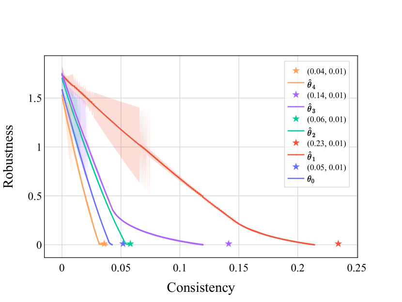
((a)) Synthetic Dataset, Logistic Regression

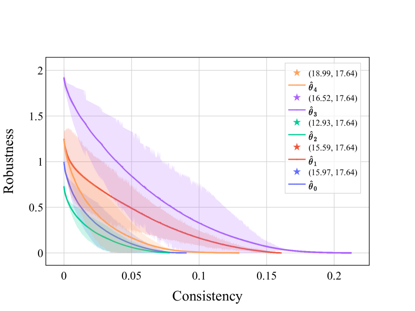
((b)) Synthetic Dataset, Neural Network

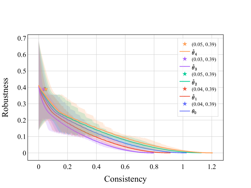
((c)) German Credit Dataset, Logistic Regression

((d)) German Credit Dataset, Neural Network

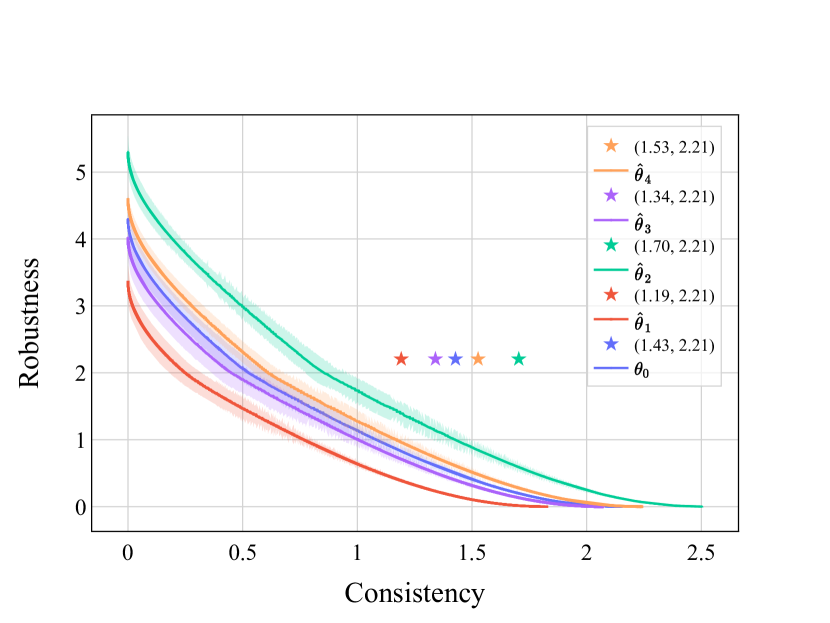
((e)) Small Business Dataset, Logistic Regression

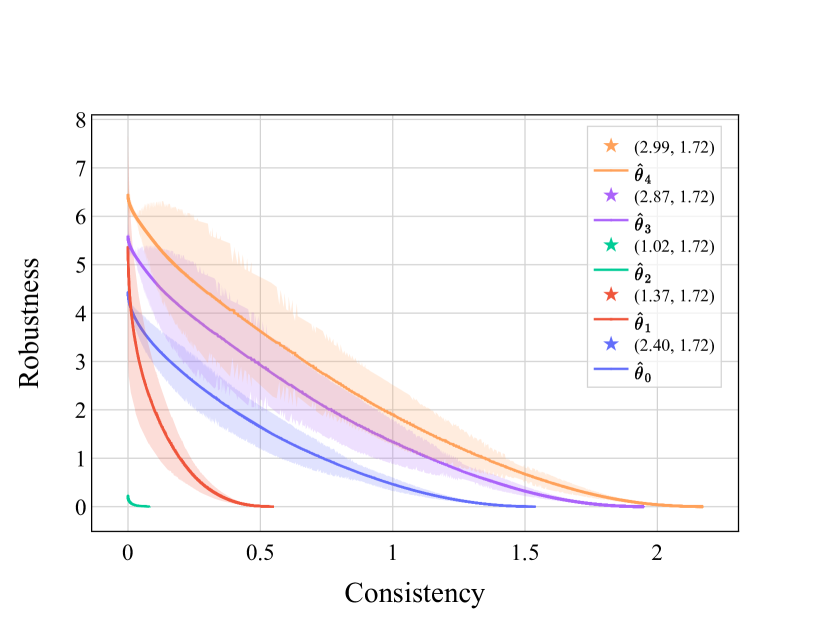
((f)) Small Business Dataset, Neural Network

Figure 4: The Pareto frontier of the trade-off between robustness and consistency for $\alpha=0.5$ with error bars for robustness: logistic regression (left) and neural network (right). Rows correspond to datasets: synthetic (top), German (middle), and Small Business (bottom). In each subfigure, each curve shows the trade-off for different predictions. The robustness and consistency of ROAR solutions are mentioned in parentheses and depicted by stars. Missing stars are outside of the range of the coordinates of the figure.

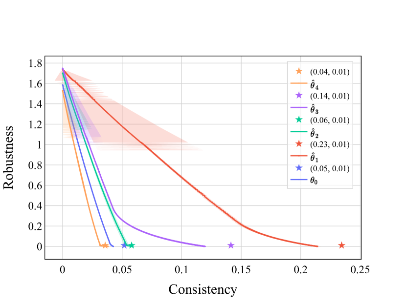
((a)) Synthetic Dataset, Logistic Regression

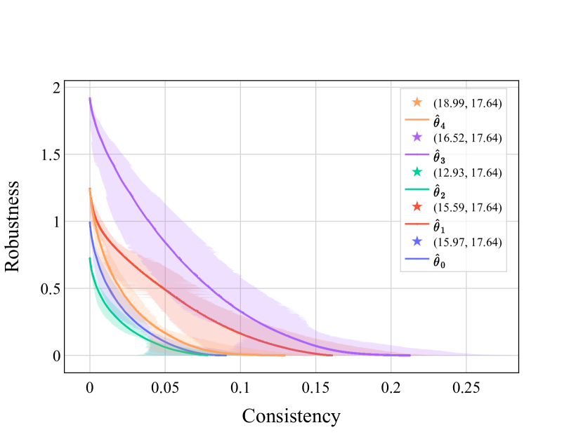
((b)) Synthetic Dataset, Neural Network

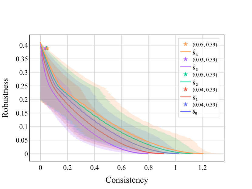
((c)) German Credit Dataset, Logistic Regression

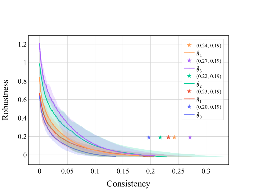
((d)) German Credit Dataset, Neural Network

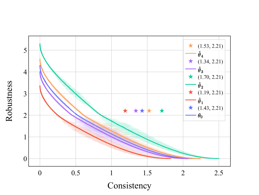
((e)) Small Business Dataset, Logistic Regression

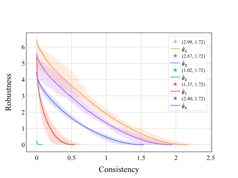
((f)) Small Business Dataset, Neural Network

Figure 5: The Pareto frontier of the trade-off between robustness and consistency for $\alpha=0.5$ with error bars for consistency: logistic regression (left) and neural network (right). Rows correspond to datasets: synthetic (top), German (middle), and Small Business (bottom). In each subfigure, each curve shows the trade-off for different predictions. The robustness and consistency of ROAR solutions are mentioned in parentheses and depicted by stars. Missing stars are outside of the range of the coordinates of the figure.

B.3 Experiments on Larger Datasets

In this section, we provide experimental results for a much larger dataset (both in terms of the number of instances and number of features) compared to the datasets in Section 4. The running time of our algorithm scales linearly with the number of instances for which recourse is provided. For each instance, the running time of our algorithm grows linearly in the number of features since the minimization problem in Line 13 of our algorithm can be solved analytically. For non-linear models, the cost of approximating the model with a linear function should be added to the total cost per instance.

We use the ACSIncome-CA [14] dataset for experiments in this section. This dataset originally consisted of 195,665 data points and 10 features, 7 of which are categorical and have been one-hot encoded. However, to lower the runtime, we sub-sampled the dataset to include 50,000 data points, and removed the categorical feature “occupation (OCCP)", as it contains more than 500 different occupations. This left us with more than 250 features after one hot encoding.

Figure 6 depicts the trade-off between the cost and validity of recourse for both logistic regression and neural network models. The choices of parameters used for results in Figure 6 are the same as the results for Figure 3 in Section 4.2. We observe that even in a dataset with a much larger number of features, Algorithm 1 can generate recourses with high validity, especially for logistic regression models. Similar to Figure 3, achieving very high validity comes at a cost of higher implementation cost which is higher than the cost required for smaller datasets. See Figure 3.

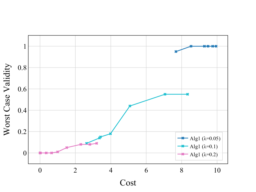
((a)) ACS Income Dataset, Logistic Regression

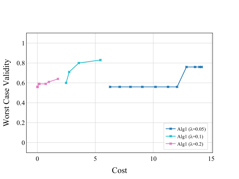
((b)) ACS Income Dataset, Neural Network

Figure 6: The Pareto frontier of the trade-off between the worst-case validity and the cost of recourse solutions. The left panel is for the logistic regression while the right panel is for a 3-layer neural network for the ACS Income dataset. In each subfigure, each curve shows the trade-off for different methods as mentioned in the legend.

B.4 Effect of the Parameters

In the experiments on the trade-off between robustness and consistency in Section 4.1 we used $\alpha=0.5$ and a $\lambda$ that maximizes the validity of recourse with respect to this $\alpha$. In this section, we see how varying $\alpha$ can affect the results. In particular, in Figures 7 and 8, we replicated the trade-offs presented in Figure 1 in Section 4.1 with $\alpha=0.1$ and $\alpha=1$, respectively. Again, for each choice of $\alpha$, we selected a $\lambda$ that maximizes the validity of recourse with respect to this $\alpha$. We generally observe that increasing $\alpha$ increases both the robustness and consistency costs.

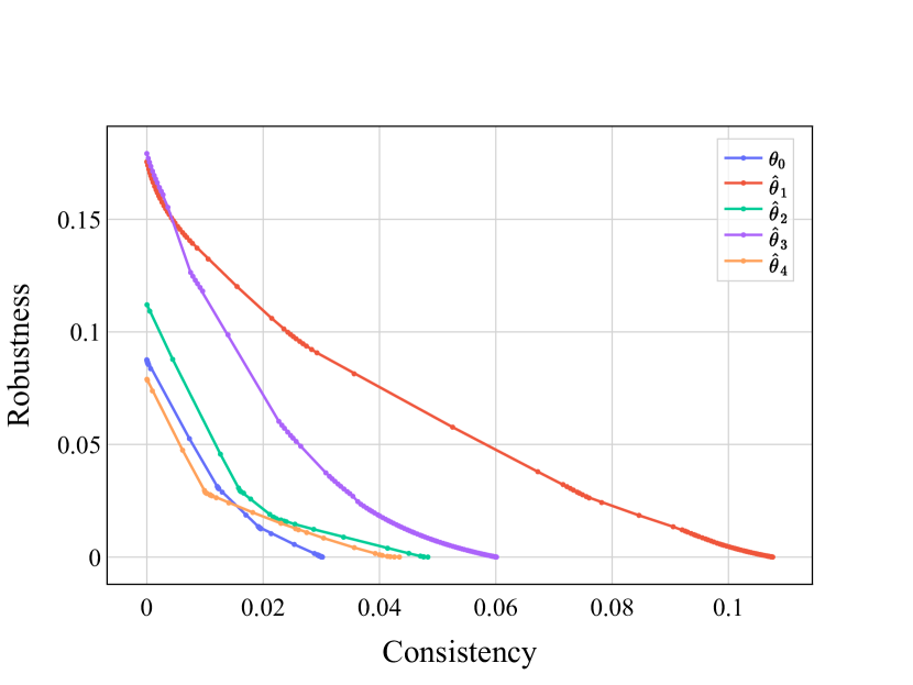
((a)) Synthetic Dataset, Logistic Regression

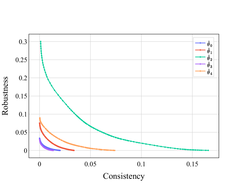
((b)) Synthetic Dataset, Neural Network

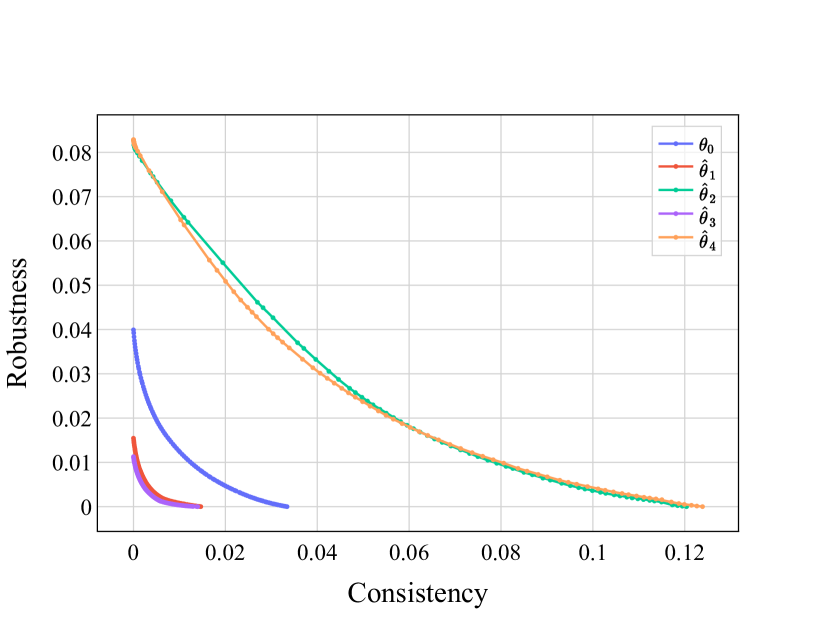
((c)) German Credit Dataset, Logistic Regression

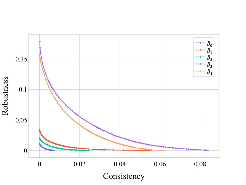
((d)) German Credit Dataset, Neural Network

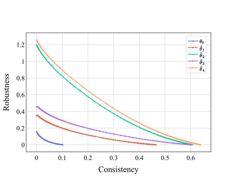
((e)) Small Business Dataset, Logistic Regression

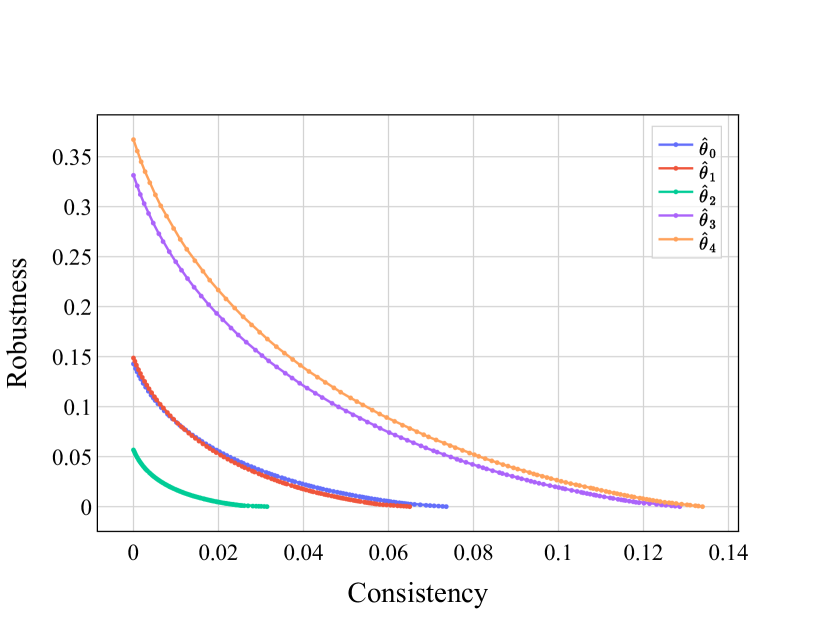
((f)) Small Business Dataset, Neural Network

Figure 7: The Pareto frontier of the trade-off between robustness and consistency for $\alpha=0.1$: logistic regression (left) and neural network (right). Rows correspond to datasets: synthetic (top), German (middle), and Small Business (bottom). In each subfigure, each curve shows the trade-off for different predictions as mentioned in the legend.

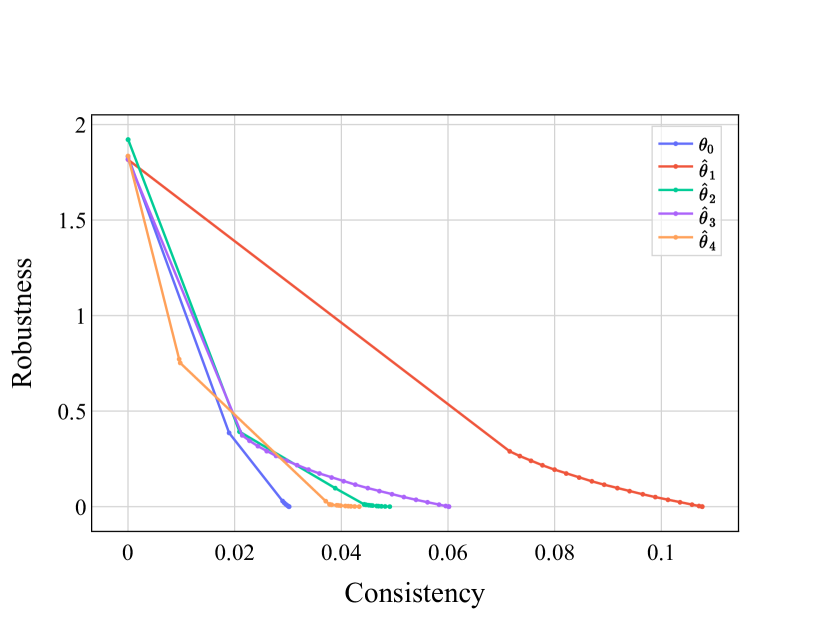
((a)) Synthetic Dataset, Logistic Regression

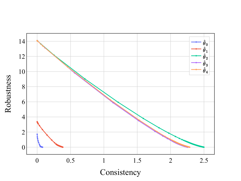
((b)) Synthetic Dataset, Neural Network

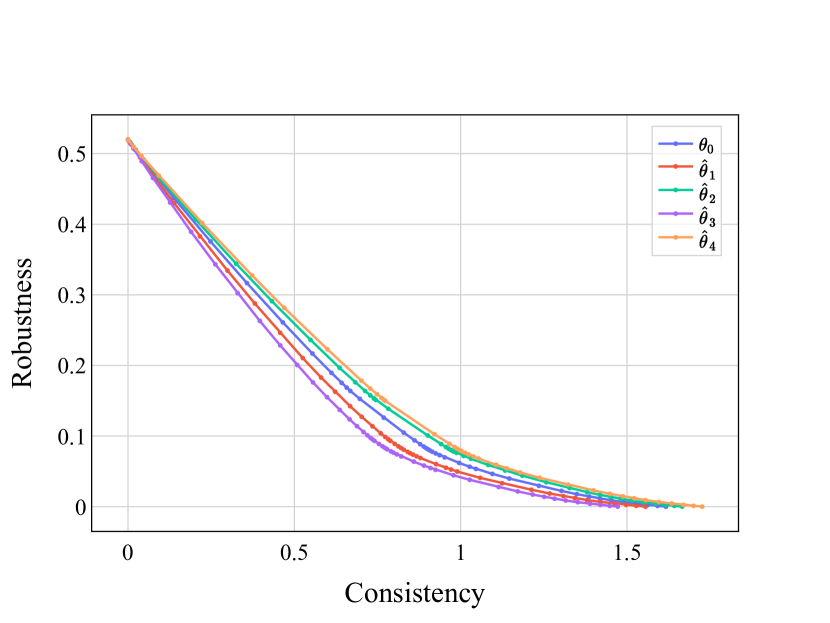
((c)) German Credit Dataset, Logistic Regression

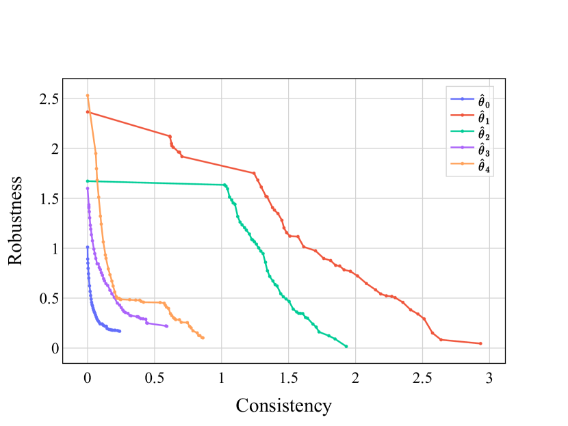
((d)) German Credit Dataset, Neural Network

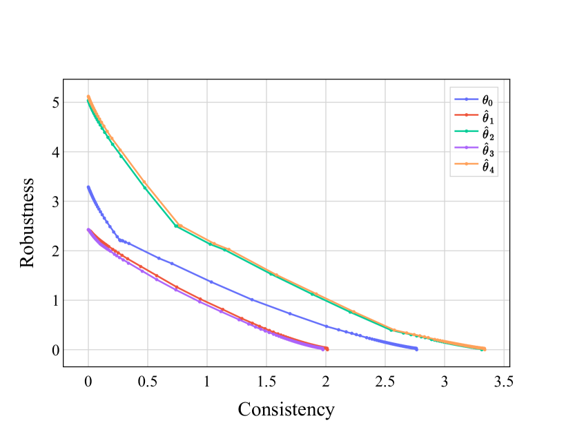
((e)) Small Business Dataset, Logistic Regression

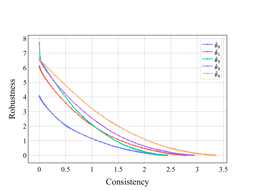
((f)) Small Business Dataset, Neural Network

Figure 8: The Pareto frontier of the trade-off between robustness and consistency for $\alpha=1$: logistic regression (left) and neural network (right). Rows correspond to datasets: synthetic (top), German (middle), and Small Business (bottom). In each subfigure, each curve shows the trade-off for different predictions as mentioned in the legend.

References

- Agarwal et al. [2021] Sushant Agarwal, Shahin Jabbari, Chirag Agarwal, Sohini Upadhyay, Steven Wu, and Himabindu Lakkaraju. Towards the unification and robustness of perturbation and gradient based explanations. In 38th International Conference on Machine Learning, 2021.
- Agrawal et al. [2022] Priyank Agrawal, Eric Balkanski, Vasilis Gkatzelis, Tingting Ou, and Xizhi Tan. Learning-augmented mechanism design: Leveraging predictions for facility location. In 23rd ACM Conference on Economics and Computation, pages 497–528, 2022.
- Athalye et al. [2018] Anish Athalye, Nicholas Carlini, and David Wagner. Obfuscated gradients give a false sense of security: Circumventing defenses to adversarial examples. In 35th International Conference on Machine Learning, pages 274–283, 2018.
- Barocas et al. [2019] Solon Barocas, Moritz Hardt, and Arvind Narayanan. Fairness and Machine Learning: Limitations and Opportunities. fairmlbook.org, 2019.
- Barocas et al. [2020] Solon Barocas, Andrew Selbst, and Manish Raghavan. The hidden assumptions behind counterfactual explanations and principal reasons. In 3rd ACM Conference on Fairness, Accountability, and Transparency, pages 80–89, 2020.
- Barshan et al. [2020] Elnaz Barshan, Marc-Etienne Brunet, and Gintare Dziugaite. RelatIF: Identifying explanatory training samples via relative influence. In 23rd International Conference on Artificial Intelligence and Statistics, pages 1899–1909, 2020.
- Bechavod et al. [2022] Yahav Bechavod, Chara Podimata, Zhiwei Steven Wu, and Juba Ziani. Information discrepancy in strategic learning. In 38th International Conference on Machine Learning, pages 1691–1715, 2022.
- Bell et al. [2024] Andrew Bell, João Fonseca, Carlo Abrate, Francesco Bonchi, and Julia Stoyanovich. Fairness in algorithmic recourse through the lens of substantive equality of opportunity. CoRR, abs/2401.16088, 2024.
- Berk et al. [2021] Richard Berk, Hoda Heidari, Shahin Jabbari, Michael Kearns, and Aaron Roth. Fairness in criminal justice risk assessments: The state of the art. Sociological Methods & Research, 50(1):3–44, 2021.
- Bewley et al. [2024] Tom Bewley, Salim Amoukou, Saumitra Mishra, Daniele Magazzeni, and Manuela Veloso. Counterfactual metarules for local and global recourse. In 41st International Conference on Machine Learning, 2024.
- Black et al. [2022] Emily Black, Zifan Wang, and Matt Fredrikson. Consistent counterfactuals for deep models. In 10th International Conference on Learning Representations, 2022.
- Boyd and Vandenberghe [2014] Stephen Boyd and Lieven Vandenberghe. Convex Optimization. Cambridge University Press, 2014.
- Cesa-Bianchi and Lugosi [2006] Nicolò Cesa-Bianchi and Gábor Lugosi. Prediction, learning, and games. Cambridge University Press, 2006.
- Ding et al. [2021] Frances Ding, Moritz Hardt, John Miller, and Ludwig Schmidt. Retiring Adult: New datasets for fair machine learning. In Advances in Neural Information Processing Systems 34, pages 6478–6490, 2021.
- Dominguez-Olmedo et al. [2022] Ricardo Dominguez-Olmedo, Amir-Hossein Karimi, and Bernhard Schölkopf. On the adversarial robustness of causal algorithmic recourse. In 39th International Conference on Machine Learning, pages 5324–5342, 2022.
- Dutta et al. [2022] Sanghamitra Dutta, Jason Long, Saumitra Mishra, Cecilia Tilli, and Daniele Magazzeni. Robust counterfactual explanations for tree-based ensembles. In 39th International Conference on Machine Learning, volume 162, pages 5742–5756, 2022.
- Ehyaei et al. [2024] Ahmad-Reza Ehyaei, Ali Shirali, and Samira Samadi. Collective counterfactual explanations via optimal transport. CoRR, abs/2402.04579, 2024.
- Fokkema et al. [2024] Hidde Fokkema, Damien Garreau, and Tim van Erven. The risks of recourse in binary classification. In 27th International Conference on Artificial Intelligence and Statistics, pages 550–558, 2024.
- Fonseca et al. [2023] João Fonseca, Andrew Bell, Carlo Abrate, Francesco Bonchi, and Julia Stoyanovich. Setting the right expectations: Algorithmic recourse over time. In 3rd ACM Conference on Equity and Access in Algorithms, Mechanisms, and Optimization, pages 29:1–29:11, 2023.
- Gao and Lakkaraju [2023] Ruijiang Gao and Himabindu Lakkaraju. On the impact of algorithmic recourse on social segregation. In 40th International Conference on Machine Learning, pages 10727–10743, 2023.
- Grömping [2020] Ulrike Grömping. South German Credit (UPDATE). UCI Machine Learning Repository, 2020. DOI: https://doi.org/10.24432/C5QG88.
- Guldogan et al. [2023] Ozgur Guldogan, Yuchen Zeng, Jy-yong Sohn, Ramtin Pedarsani, and Kangwook Lee. Equal improvability: A new fairness notion considering the long-term impact. In 11th International Conference on Learning Representations, 2023.
- Guo et al. [2023] Hangzhi Guo, Feiran Jia, Jinghui Chen, Anna Squicciarini, and Amulya Yadav. RoCourseNet: Robust training of a prediction aware recourse model. In 32nd ACM International Conference on Information and Knowledge Management, pages 619–628. ACM, 2023.
- Gupta et al. [2019] Vivek Gupta, Pegah Nokhiz, Chitradeep Roy, and Suresh Venkatasubramanian. Equalizing recourse across groups. CoRR, abs/1909.03166, 2019.
- Hamman et al. [2023] Faisal Hamman, Erfaun Noorani, Saumitra Mishra, Daniele Magazzeni, and Sanghamitra Dutta. Robust counterfactual explanations for neural networks with probabilistic guarantees. In 40th International Conference on Machine Learning, pages 12351–12367, 2023.
- Hardt et al. [2016] Moritz Hardt, Eric Price, and Nathan Srebro. Equality of opportunity in supervised learning. In 30th Annual Conference on Neural Information Processing Systems, pages 3315–3323, 2016.
- Heidari et al. [2019] Hoda Heidari, Vedant Nanda, and Krishna Gummadi. On the long-term impact of algorithmic decision policies: Effort unfairness and feature segregation through social learning. In 36th International Conference on Machine Learning, pages 2692–2701, 2019.
- Hofmann [1994] Hans Hofmann. Statlog (German Credit Data). UCI Machine Learning Repository, 1994. DOI: https://doi.org/10.24432/C5NC77.
- Joshi et al. [2019] Shalmali Joshi, Oluwasanmi Koyejo, Warut Vijitbenjaronk, Been Kim, and Joydeep Ghosh. Towards realistic individual recourse and actionable explanations in black-box decision making systems. CoRR, abs/1907.09615, 2019.
- Kanamori et al. [2024] Kentaro Kanamori, Takuya Takagi, Ken Kobayashi, and Yuichi Ike. Learning decision trees and forests with algorithmic recourse. In 41st International Conference on Machine Learning, 2024.
- Karimi et al. [2020a] Amir-Hossein Karimi, Gilles Barthe, Borja Balle, and Isabel Valera. Model-agnostic counterfactual explanations for consequential decisions. In 23rd International Conference on Artificial Intelligence and Statistics, pages 895–905, 2020a.
- Karimi et al. [2020b] Amir-Hossein Karimi, Bodo Julius von Kügelgen, Bernhard Schölkopf, and Isabel Valera. Algorithmic recourse under imperfect causal knowledge: a probabilistic approach. In Advances in Neural Information Processing Systems 33, 2020b.
- Khodak et al. [2023] Mikhail Khodak, Kareem Amin, Travis Dick, and Sergei Vassilvitskii. Learning-augmented private algorithms for multiple quantile release. In 40th International Conference on Machine Learning, volume 202, pages 16344–16376, 2023.
- Koh and Liang [2017] Pang Wei Koh and Percy Liang. Understanding black-box predictions via influence functions. In 34th International Conference on Machine Learning, pages 1885–1894, 2017.
- Kraska et al. [2018] Tim Kraska, Alex Beutel, Ed Chi, Jeffrey Dean, and Neoklis Polyzotis. The case for learned index structures. In International Conference on Management of Data, pages 489–504, 2018.
- Lakkaraju et al. [2016] Himabindu Lakkaraju, Stephen Bach, and Jure Leskovec. Interpretable decision sets: A joint framework for description and prediction. In 22nd ACM SIGKDD International Conference on Knowledge Discovery and Data Mining, pages 1675–1684, 2016.
- Lindermayr and Megow [2024] Alexander Lindermayr and Nicole Megow. Algorithms with predictions, 2024. URL https://algorithms-with-predictions.github.io/.
- Looveren and Klaise [2021] Arnaud Van Looveren and Janis Klaise. Interpretable counterfactual explanations guided by prototypes. In Machine Learning and Knowledge Discovery in Databases, pages 650–665, 2021.
- Lundberg and Lee [2017] Scott Lundberg and Su-In Lee. A unified approach to interpreting model predictions. In Advances in Neural Information Processing Systems 30, pages 4765–4774, 2017.
- Lykouris and Vassilvitskii [2018] Thodoris Lykouris and Sergei Vassilvitskii. Competitive caching with machine learned advice. In 35th International Conference on Machine Learning, pages 3302–3311, 2018.
- Madry et al. [2018] Aleksander Madry, Aleksandar Makelov, Ludwig Schmidt, Dimitris Tsipras, and Adrian Vladu. Towards deep learning models resistant to adversarial attacks. In 6th International Conference on Learning Representations, 2018.
- Min Li and Taylor [2018] Amy Mickel Min Li and Stanley Taylor. “should this loan be approved or denied?”: A large dataset with class assignment guidelines. Journal of Statistics Education, 26, 2018.
- Mitzenmacher and Vassilvitskii [2020] Michael Mitzenmacher and Sergei Vassilvitskii. Algorithms with predictions. In Tim Roughgarden, editor, Beyond the Worst-Case Analysis of Algorithms, pages 646–662. Cambridge University Press, 2020.
- Nguyen et al. [2022] Tuan-Duy Nguyen, Ngoc Bui, Duy Nguyen, Man-Chung Sue, and Viet Anh Nguyen. Robust bayesian recourse. In 38th Conference on Uncertainty in Artificial Intelligence, pages 1498–1508, 2022.
- Pawelczyk et al. [2020] Martin Pawelczyk, Klaus Broelemann, and Gjergji Kasneci. Learning model-agnostic counterfactual explanations for tabular data. In 29th The ACM Web Conference, pages 3126–3132, 2020.
- Pawelczyk et al. [2022] Martin Pawelczyk, Chirag Agarwal, Shalmali Joshi, Sohini Upadhyay, and Himabindu Lakkaraju. Exploring counterfactual explanations through the lens of adversarial examples: A theoretical and empirical analysis. In 25th International Conference on Artificial Intelligence and Statistics, pages 4574–4594, 2022.
- Pawelczyk et al. [2023a] Martin Pawelczyk, Teresa Datta, Johannes van den Heuvel, Gjergji Kasneci, and Himabindu Lakkaraju. Probabilistically robust recourse: Navigating the trade-offs between costs and robustness in algorithmic recourse. In 11th International Conference on Learning Representations, 2023a.
- Pawelczyk et al. [2023b] Martin Pawelczyk, Tobias Leemann, Asia Biega, and Gjergji Kasneci. On the trade-off between actionable explanations and the right to be forgotten. In 11th International Conference on Learning Representations, 2023b.
- Purohit et al. [2018] Manish Purohit, Zoya Svitkina, and Ravi Kumar. Improving online algorithms via ML predictions. In Advances in Neural Information Processing Systems 31, pages 9684–9693, 2018.
- Rawal and Lakkaraju [2020] Kaivalya Rawal and Himabindu Lakkaraju. Beyond individualized recourse: Interpretable and interactive summaries of actionable recourses. In Advances in Neural Information Processing Systems 33, 2020.
- Ribeiro et al. [2016] Marco Túlio Ribeiro, Sameer Singh, and Carlos Guestrin. “Why should I trust you?": Explaining the predictions of any classifier. In 22nd ACM SIGKDD International Conference on Knowledge Discovery and Data Mining, pages 1135–1144, 2016.
- Rudin [2019] Cynthia Rudin. Stop explaining black box machine learning models for high stakes decisions and use interpretable models instead. Nat. Mach. Intell., 1(5):206–215, 2019.
- Selvaraju et al. [2017] Ramprasaath Selvaraju, Michael Cogswell, Abhishek Das, Ramakrishna Vedantam, Devi Parikh, and Dhruv Batra. Grad-CAM: Visual explanations from deep networks via gradient-based localization. In 16th IEEE International Conference on Computer Vision, pages 618–626, 2017.
- Slack et al. [2021] Dylan Slack, Anna Hilgard, Himabindu Lakkaraju, and Sameer Singh. Counterfactual explanations can be manipulated. In Advances in Neural Information Processing Systems 34, pages 62–75, 2021.
- Smilkov et al. [2017] Daniel Smilkov, Nikhil Thorat, Been Kim, Fernanda Viégas, and Martin Wattenberg. Smoothgrad: removing noise by adding noise. CoRR, abs/1706.03825, 2017.
- Sundararajan et al. [2017] Mukund Sundararajan, Ankur Taly, and Qiqi Yan. Axiomatic attribution for deep networks. In 34th International Conference on Machine Learning, pages 3319–3328, 2017.
- Upadhyay et al. [2021] Sohini Upadhyay, Shalmali Joshi, and Himabindu Lakkaraju. Towards robust and reliable algorithmic recourse. In Advances in Neural Information Processing Systems 34, pages 16926–16937, 2021.
- Ustun et al. [2019] Berk Ustun, Alexander Spangher, and Yang Liu. Actionable recourse in linear classification. In 3rd AMC Conference on Fairness, Accountability, and Transparency, pages 10–19, 2019.
- Venkatasubramanian and Alfano [2020] Suresh Venkatasubramanian and Mark Alfano. The philosophical basis of algorithmic recourse. In 3rd ACM Conference on Fairness, Accountability, and Transparency, pages 284–293, 2020.
- Verma et al. [2020] Sahil Verma, John Dickerson, and Keegan Hines. Counterfactual explanations for machine learning: A review. CoRR, abs/2010.10596, 2020.
- Wachter et al. [2018] Sandra Wachter, Brent Mittelstadt, and Chris Russell. Counterfactual explanations without opening the black box: automated decisions and the GDPR. Harvard Journal of Law and Technology, 31(2):841–887, 2018.
- Wang et al. [2017] Tong Wang, Cynthia Rudin, Finale Doshi-Velez, Yimin Liu, Erica Klampfl, and Perry MacNeille. A bayesian framework for learning rule sets for interpretable classification. J. Mach. Learn. Res., 18:70:1–70:37, 2017.
- Wong and Kolter [2018] Eric Wong and Zico Kolter. Provable defenses against adversarial examples via the convex outer adversarial polytope. In 35th International Conference on Machine Learning, pages 5283–5292, 2018.
- Xu and Lu [2022] Chenyang Xu and Pinyan Lu. Mechanism design with predictions. In 31st International Joint Conference on Artificial Intelligence, pages 571–577, 2022.
- Yang et al. [2017] Hongyu Yang, Cynthia Rudin, and Margo Seltzer. Scalable bayesian rule lists. In Doina Precup and Yee Whye Teh, editors, 34th International Conference on Machine Learning, pages 3921–3930, 2017.
- Zafar et al. [2017] Muhammad Zafar, Isabel Valera, Manuel Gomez-Rodriguez, and Krishna P. Gummadi. Fairness constraints: Mechanisms for fair classification. In 20th International Conference on Artificial Intelligence and Statistics, pages 962–970, 2017.